extreme man-made and natural hazards in dynamics of...
TRANSCRIPT

Extreme Man-Made and Natural
Hazards in Dynamics of Structures
edited by
Adnan IbrahimbegovicEcole Normale Supérieure de Cachan,
France
and
Ivica KozarUniversity of Rijeka,
Croatia
Published in cooperation with NATO Public Diplomacy Division

Proceedings of the NATO Advanced Research Workshop on
Extreme Man-Made and Natural Hazards in Dynamics of Structures
Opatija, Croatia
28 May - 1 June 2006
A C.I.P. Catalogue record for this book is available from the Library of Congress.
ISBN-10 1-4020-5655-9 (PB)
ISBN-13 978-1-4020-5655-0 (PB)
ISBN-10 1-4020-5654-0 (HB)
ISBN-13 978-1-4020-5654-3 (HB)
ISBN-10 1-4020-5656-7 (e-book)
ISBN-13 978-1-4020-5656-7 (e-book)
Published by Springer,
P.O. Box 17, 3300 AA Dordrecht, The Netherlands.
www.springer.com
Printed on acid-free paper
All Rights Reserved
© 2007 Springer
No part of this work may be reproduced, stored in a retrieval system, or transmitted in
any form or by any means, electronic, mechanical, photocopying, microfilming,
recording or otherwise, without written permission from the Publisher, with the exception
of any material supplied specifically for the purpose of being entered and executed on a
computer system, for exclusive use by the purchaser of the work.

Part I: Numerical modelling and dynamics of complex structures
‘Computational issues in the simulation of blast
and impact problems: An industrial perspective’
A. Ibrahimbegovic, D. Brancherie, J-B. Colliat, L. Davenne,
Nonlinear transient analysis, testing and design
of complex engineering structures for worst case accidents:
Experience from industrial and military applications’
‘On reliable finite element methods for extreme loading conditions’
of probability and applications’
‘Optimum performance-based reliability design of structures’
Part III: Fire and explosion induced extreme loading conditions
‘Computational modelling of safety critical concrete structures
at elevated temperatures’
‘Three-dimensional FE analysis of headed stud anchors
exposed to fire’
Part IV: Fluid flow induced extreme loading conditions
F. Dias, D. Dutykh ………….……………………………….…………. 201 ‘Dynamics of tsunami waves’
TABLE OF CONTENTS
.,
Part II: Probability aspects, design and uncertainty
‘Quantifying uncertainty:Modern computational representation
D.R.J. Owen, Y.T. Feng, M.G. Cottrell, J. Yu ………..…………………... 3
N. Dominguez, G. Herve, P. Villon………...…...……………………….. 3 7
.
K.J. Bathe,…..…..…………………………………………………………71
H.G. Matthies ………...……….………………..…………………….….105
P. Papadrakakis, M. Fragiadakis, N. Lagaros ……………..………….....137
N. Bicanic, C. Pearce, C. Davie ……………………………………....…163
J. Ozbolt, I. Kozar, G. Periski …………………...…………...……..…...177

‘Modelling fluid-induced structural vibrations: Reducing
the structural risk for stormy winds’
Part V: Earthquake induced extreme loading conditions
P. Fajfar ...…………………..…………………………………………... 257 ‘Seismic assessment of structures by a practice-oriented method’
P. Leger …………….…………………………………………………... 285
in monumental structures: Experience at Ecole Polytechnique
de Montreal for large concrete dams supported
by Hydro-Quebec and Alcan’
F.J. Molina, M. Geradin …………………………...…………………… 311 ‘Earthquake engineering experimental research at JRC-ELSA’
‘The history of earthquake engineering at the University
of California Berkeley and recent developments
of numerical methods and computer programs at CSI Berkeley’
Appendix: Statistics on extreme loading conditions for Croatia
‘Security issues in Croatian construction industry: Bases
of statistical data for quantifying extreme loading conditions’
iv TABLE OF CONTENTS
‘Reducing the earthquake induced damage and risk
D. Peric, W.D. Dettmer, P.H. Saksono…..……………………………... 225
E.L. Wilson ……………………..…………………..……………...……353
P. Marovic, V. Herak-Marovic ………………………………………….383
Author index ………………….………………….……………………..397

There is currently ever pressing need to provide a critical assessment of the current knowledge and indicate new challenges which are brought by the present time in fighting the man-made and natural hazards in transient analysis of structures. The latter concerns both the permanently fixed structures, such as those built to protect the people and/or sensitive storage material (e.g. military installations) or the special structures found in transportation systems (e.g. bridges, tunnels), and the moving structures (such as trains, plains, ships or cars). The present threat of the terrorist attacks or accidental explosions, the climate change which brings strong stormy winds or yet the destructive earthquake motion that occurs in previously inactive regions or brings about tsunamis, are a few examples of the kind of applications we seek to address in this work. The common ground for all the problems of this kind from the viewpoint of structural integrity, which also justifies putting them on the same basis and addressing them within the same context, is their sudden appearance, their transient nature and the need to evaluate the consequence for a high level of uncertainty in quantifying the cause. The problems of such diversity cannot be placed within a single traditional scientific discipline, but they call for the expertise in probability theory for quantifying the cause, interaction problems for better understanding the physical nature of the problems, as well as modeling and computational techniques for improving the representation of inelastic behavior mechanisms and providing the optimal design. The present time of high uncertainty is very likely to increase (rather than decrease) the frequency or severe intensity of the high-risk situations that a very few engineering structures have been built to sustain. It is therefore important to understand any potential reserve, which might exist in engineering structures for taking on a higher level of risk. The complementary goal, also of great importance, pertains to providing the best way of reducing the negative impact of high-risk situations that cannot be avoided, by resorting to a more sound design procedure. Never before have we had the same level of development of scientific and technological achievements, which can be brought to bear on the present problem of high complexity. First, the constant progress in computational tools ought to be exploited to construct the more refined structure models than those used previously, which can provide a more detailed information and explore all potential reserves in a more old-fashioned design. Second, one can nowadays understand much better the particular physical nature of the loading conditions, by simulating the actual physical process that is at its origin, and in that manner providing a more reliable estimate of the parameters governing the processes of this kind. The quantitative information can be bracketed between the probabilistic bounds,
PREFACE

which can nowadays be constructed for more and more complex processes, thanks to significant advances in modern computational probability research. The present work is the outcome of a lively exchange of ideas among the world leading scientists dealing with different facets of this class of complex problems. Among them, specialists in probability, in structural engineering, in interaction problems and in development of computer models, as well as related experimental works, have all contributed to the successful accomplishment of the hazard reduction goal set for our meeting. The lectures presented in this book are regrouped on any single topic to provide the most detailed presentations, seeking to reach eventually complementary points of view. A fair number of pages is allocated to each chapter in order to provide the complete presentation of any given facet of the problem and a sufficiently detailed exposition to any important idea to be grasped. Among several illustrative applications which are discussed herein we find: quantifying the plane-crash or explosion induced impact loading, quantifying the effects of a strong earthquake motion, quantifying the impact and long-duration effects of strong stormy winds, providing the most efficient tools to construct the probabilistic bounds and computational tools for probabilistic analysis, constructing refined models for nonlinear dynamic analysis and optimal design and presenting modern computational tools for that purpose. All the papers collected in this book are first presented as the keynote lectures at NATO-ARW NNoo.. 998811664411,, which was held in the city of Opatija in Croatia, from May 28 to June 1, 2006. We would like to thank all the participants for their important contributions to the successful outcome of this meeting, and in particular to the keynote lecturers, Professors K.J.
Leger, H.G. Matthies,, D.R.J Owen, M. Papadrakakis, D. Peric and E.L. Wilson, for ensuring a more lasting impact of this meeting in terms of the present book. Last but not least, we would also like to thank NATO Science Committee for selecting our meeting, NATO-ARW NNoo.. 998811664411,, for the financial support by NATO.
NATO-country co-director: Partner country co-director:Professor Adnan Ibrahimbegovic Professor Ivica Kozar ENS-Cachan, Paris, France FGZ-Rijeka, Croatia
viii PREFACE
Bathe, N. Bicanic, F. Dias, P. Fajfar, M. Geradin, A. Ibrahimbegovic, P.

Part V: EARTHQUAKE INDUCED EXTREME LOADING CONDITION

EARTHQUAKE ENGINEERING EXPERIMENTAL RESEARCH AT
JRC-ELSA
*
Joint Research Centre (Ispra, I), European Commission ELSA Laboratory, 21020 Ispra (Varese), Italy
Abstract: The ELSA laboratory is equipped with a large reaction-wall facility and has acquired its best expertise on the development and implementation of innovative experimental techniques mainly related to testing large-scale specimens by means of the pseudodynamic method. Apart from the relevant achievements within the testing techniques, such as the continuous pseudodynamic test and the development of effective techniques for the assessment of the experimental errors, the role of a reference laboratory in Europe has allowed ELSA to rely on the collaboration of many important research institutions that have contributed through the projects with and added maximum scientific value to the results of the tests. An example of pioneering tests performed for a relevant collaborative project are represented by the bi-directional tests performed on a multi-storey building, where the combination of sophisticated techniques have allowed for the first time to obtain most valuable information on the seismic experimental response of a torsionally unbalanced existing building in its original and retrofitted configurations.
bidirectional test, torsional response.
1. Introduction
During the last two decades, the pseudodynamic (PsD) method has increasingly been used for seismic testing of structures. The reason for this has been the possibility of testing large-scale constructions or substructures in clear advantage with respect to shaking table testing. Testing large specimens or sub-assemblages in laboratory represents of course a way to complement the lessons obtained from
F. Javier Molina and M. Géradin ([email protected])
Key words : Dynamic test, seismic test, pseudodynamic test, reaction wall, control errors,
311
A. Ibrahimbegovic and I. Kozar (eds.),Extreme Man-Made and Natural Hazards in Dynamics of Structures, 311–351. © 2007 Springer.
F.J. MOLINA AND M. GERADIN
the behaviour of real constructions during natural earthquakes. During these years, the European Laboratory for Structural Assessment (ELSA) has substantially contributed to new developments within the PsD methodology thanks to a proper in-house design of hardware and software in which high accuracy sensors and devices are used under a flexible architecture with a fast intercommunication among the controllers. The loading capabilities of ELSA’s reaction wall are shown in Figure 1 (Donea et al., 1996).
The PsD method is an hybrid technique by which the seismic response of large-size specimens can be obtained by means of the on-line combination of experimental restoring forces with analytical inertial and seismic-equivalent forces (Takanashi an Nakashima, 1986). Thanks to the use of quasistatic imposed displacements, the accuracy of the control and hence the quality of such test is normally better than for a shaking-table test, especially for heavy and tall specimens. In the classical version of the PsD method, displacements are applied stepwise allowing the specimen to stabilise at every step (subsection 2.1). The quality of the test can be further improved using a continuous version of the method as will be described in subsection 2.2. In any case, it is important to recognise that the PsD method is a sophisticated tool that may fail or produce inaccurate results in some cases depending on the systematic experimental errors (Shing and Mahin, 1987, Molina et al., 2002). Particularly, it is well known that the slight phase lags of the control system, which is used to quasi-statically deform the specimen, may considerably distort the apparent damping characteristics of the PsD response and artificially excite the higher modes (subsection 3.1). The ELSA team has undergone many relevant PsD tests, most of which have been used for the improvement of EC8 and the assessment of several categories of structures. Taking advantage of this activity, various analysis techniques have been developed and applied that try to assess the magnitude and consequences of the existing experimental errors (subsection 3.2). Some of these techniques are based on the identification of linear models using a short-time portion of the response. The identified parameters are then transformed into frequency and damping characteristics. By gaining experience in the application of these analysing techniques, it is possible to have a better knowledge of what the feasibility and the accuracy of the experiment can be depending on the type of structure and the applied PsD testing set-up.
The example of application described at section 4 of this chapter refers to the SPEAR project. There, ELSA has performed accurate bidirectional PsD tests on a real-size multi-storey building specimen by using up to nine DoFs and twelve
312

EARTHQUAKE ENGINEERING EXPERIMENTS AT JRC-ELSA
Figure 1. Dimensions and capacities of the reaction wall-strong floor system at ELSA.
actuators plus sophisticated geometric and static on-line transformations of variables between the equation of motion and the controllers. The results of these tests have widened the knowledge on the torsional response of plan-wise irregular buildings.
Out of the scope of this work, a different line of application is also worth mentioning, i.e. the use of the PsD method on structures seismically protected by passive isolators or dissipators. In such applications involving new materials and/or devices, the strain rate effect can become significant. Such effect should be reduced there by increasing the testing speed if possible and by an analytical on-line compensation of it when appropriate (De Luca et al., 2001, Molina et al., 2002b, 2004). Also important to mention are the substructuring techniques developed within the PsD method, which have proved to be very useful for obtaining the seismic response of large structures such as bridges. In that case, a testing set-up is devised in which the reduced part of the structure that has the strongest non-linear behaviour (typically some of the piers) is the actual specimen and the rest of the structure (the deck and the remaining piers) is numerically substructured (Pinto et al., 2004). In a different field of research, an important activity of ELSA is also dedicated to real dynamic tests oriented to the
313

F.J. MOLINA AND M. GERADIN
development of active-control systems, such as the case of attenuation of vibration on bridges (Magonette et al., 2003), vibration monitoring for damage detection or fatigue testing on large cable specimens. The common denominator of all these tests has been the use of innovative testing techniques or the development of advanced structural systems.
Finally, during the last years ELSA has also put an important effort in the development of techniques for telepresence, teleoperation and, in general, distributed laboratory environment, which have been successful and now are becoming compatible with the Network for Earthquake Engineering Simulation (NEES) (Pinto et al., 2006). NEES currently integrates the major US laboratories, making it possible for researchers to collaborate remotely on experiments, computational modelling, and education.
2. Implementation of the Pseudodynamic Test Method
PsD testing consists of the step-by-step integration of the discrete-DoF equation of motion
TMa r(d) f( ) (1)
where M is the theoretical matrix of mass, a and d represent the unknown vectors of acceleration and displacement and Tf( ) are known external forces that, in the case of a seismic excitation, are obtained by multiplying the specified ground acceleration by the theoretical masses. The unknown restoring forces r(d) are experimentally obtained at every integration step by quasistatically imposing, generally by means of a hydraulic control system, the computed displacements.
For every PsD test, we will define the prototype time T (Figure 2), which corresponds to the one of the original problem with an earthquake excitation that may last for a few tens of seconds, and the experimental time t , which may extend to several hours for the execution of the test in the laboratory. We may call the time scale factor, defined as the proportion between experimental and prototype times, i.e.,
t
T(2)
that usually ranges from one hundred to a few thousands.
314

EARTHQUAKE ENGINEERING EXPERIMENTS AT JRC-ELSA
2.1. CLASSICAL STEPWISE PSD METHOD
In the classical PsD method, the time increment T for the integration of the equation of motion is chosen small enough to satisfy the stability and accuracy criteria of the integration scheme. The ground accelerogram must be discretised with the prototype record increment (Figure 2). The smaller this time increment is chosen, the larger the number of integration steps will be to cover the duration of the earthquake. The execution of every step will take place in the corresponding experimental time lapse t , which uses to be in the order of several seconds. In fact, the experimental time t is split in four phases (Figure 2):
1. A stabilising hold period 1ht of the system motion after the ramp of the reference signal at the controller. In practise, this period allows the specimen to reach the computed displacement. If the computed displacement has not been accurately achieved, the measured force will not correspond to the computed displacement.
2. A measuring hold period 2ht that allows reducing the signal noise by averaging a number of measures. This could be important to reduce some random errors in the solution.
3. A computation hold period 3ht for solving the next step at the integration algorithm. This period includes also the transmission time if the system equations are solved in a different CPU than the controller itself.
4. A period of ramp rampt at the reference signal in order to smoothly change to the new computed displacement 1nd -- during the three previous hold periods, the reference was maintained constant at the previous value of the computed displacement nd .
The accuracy in the imposed displacement and the measured force depends, apart from the characteristics of the experimental set-up, on the selected periods for stabilising, measuring and ramp, while the computation period is determined by the system equations and processor characteristics.
2.2. CONTINUOUS PSD METHOD
In the continuous PsD method (Figure 3), as a difference with respect to the classical one, the execution of every integration step takes just one sampling period (S.P.) of the digital controller of the control system, e.g. 2 ms in the ELSA implementation (Magonette et al., 1998). The ramp and stabilising periods are
315

F.J. MOLINA AND M. GERADIN
reduced to zero duration and the measuring plus the computation periods must be feasible within those few milliseconds of experimental time. The surprising fact is that, since the hydraulic control system is unable to respond significantly at frequencies in the range of the sampling frequency of its controller, e.g. 500 Hz, the missing periods of ramp and stabilising are not needed at all. Under these conditions, the accuracy in the imposed displacement depends basically on the testing speed, which is characterised by the time scale factor (Eq. 2). In order to reduce the testing speed while the experimental time step is kept fixed to one S.P., every original time increment in the prototype domain is subdivided into a number of internal steps intN (Figure 3), so that, by increasing this number, the time scale factor is enlarged as
int S.P.t N
T T (3)
As shown in Figure 3, at every T the required internal values of the input ground accelerogram are linearly interpolated from the original record values. The total number of integration steps in a continuous PsD test can be of several millions, in comparison with several thousands as typically required for a classical PsD test for the same specified earthquake. This fact implies that, on the one hand, an explicit time integration algorithm can always be used without concern about stability or integration error and, on the other hand, there is no longer need for an averaging period at the measuring of the force since any high-frequency noise at the load cells will automatically be filtered out in the solution. Such filtering effect is due to the equation response characteristics for the frequency associated to such small time increment.
Additionally, working with the continuous PsD method, it is usually possible to perform the test in a shorter experimental time, but with a better accuracy than with the classical method for the same experimental hardware. This is because, as a consequence of the mentioned characteristics of the continuous version, the absence of alternation between ramp and hold periods in the controller reference signal notably improves the control quality.
3. Assessment of Experimental Errors in Pseudodynamic Tests
The experimental errors within the PsD method can be of different types (Shing and Mahin, 1987) and may come from a lack of reliability of the used instruments as well as from the limitations in the adopted discrete model, which obviously includes a discrete mass representation, and the strain-rate effects coming from the slow application of the load. However, the kind of errors whose effects are the most difficult, in principle, to predict are the ones coming from the control
316

EARTHQUAKE ENGINEERING EXPERIMENTS AT JRC-ELSA
system. In this section we will concentrate on this type of error that can be critical for the success of any PsD test.
3.1. LINEAR MODEL OF THE TESTING SET-UP
The development of a linear model of the testing set-up including the specimen and the hydraulic system can be a very helpful tool for understanding the effects of the experimental errors in a PsD test. For an ideal case without control errors, running the test with a time scale factor of , the history of every variable in the experimental response should equal the one of the prototype except for the time scale. For example, that means that, in the time t of the laboratory, the experimental response eigenmodes and damping ratios would be the same as for the prototype structure but the eigenfrequencies will be times smaller than in the prototype (Molina et al., 2002a):
Figure 2. Classical stepwise PsD method.
T
Prototype time T
Ground accelerogramag n
ag
t = T
Experiment time t
Specimen
dndn+1
trath2 th3th1
reference
measured
317

F.J. MOLINA AND M. GERADIN
Figure 3. Continuous PsD method.
;id idn
n n nt t (4)
In the presence of errors introduced by the hydraulic system, the obtained experimental frequencies and damping ratios will differ from the ideal ones so that respective associated errors can be defined as
;id
idn nt tn nid t t
n t
(5)
Using the proposed linear model, the behaviour of these errors can be analysed as a function of the characteristic of the set-up components, such as the pistons and servovalves dimensions, and the testing parameters. The testing speed and the controller proportional gain are among the testing parameters that most strongly may influence the accuracy of the test. In the case of the classical version
TPrototype time T
Ground accelerogram ag n
ag
T/Ni
Experiment time t
Specimen
dndn+1
reference measured
S.P.
t = T = Nint
318

EARTHQUAKE ENGINEERING EXPERIMENTS AT JRC-ELSA
of the method, the selected hold and ramp periods (Figure 2) may also be determinant, but here we will concentrate our study on the continuous version of the method. An example of this type of analysis will be shown here. In this example (Figure 4), a piston deforms a single-DoF specimen with prototype mass of 4150 kg, eigenfrequency
2.5n Hz (6)
and damping ratio
0.10n (7)
In practice, the tested specimens generally exhibit hysteretic damping, in which case this parameter must be understood as a “viscous-equivalent” damping ratio. However, within the model, the damping of the specimen is of viscous type with a damping constant inversely proportional to the testing speed. This scheme allows having a damping force that does not change with the time scale as one can expect from hysteretic damping behaviour.
Figure 4. Example of PsD set-up with a single DoF specimen.
The model will include a proportional controller and an ideal linear servovalve. The compliance of the oil column inside the cylinder will be considered by means of a linear spring of 5·107 N/m and the internal friction in the cylinder by a linear damper of 6·104 Ns/m. The mass of the piston moving with the specimen mass will be 67.5 kg.
specimen( ,n n
)
actuator
319

F.J. MOLINA AND M. GERADIN
Initially, the proportional gain of the controller-servovalve-piston set is given a value of
12.5conP s (8)
defined within this model in terms of piston theoretical velocity (for uncompressible oil) divided by displacement error.
The results of the application of the model to a continuous PsD test at different testing speeds are shown in Table and Figure 5. If the test is performed at a speed times slower than the reality (see the first column at the table), the ideal value of the response frequency and damping in the laboratory time are given by Eq. (4). The ideal frequency is given at the second column of the table while the ideal damping ratio is 0.10 for all the cases. The response eigenfrequency and damping ratio as obtained by solving the described PsD linear model during the test are shown at columns 4 and 5. The respective error measures on the eigenfrequency and damping are also shown at columns 6 and 7. It is clearly seen that their values grow with the testing speed.
Table 1. PsD test example at several testing speeds.
(id
n tH conP ( )n t
Hzn t
i
n nt tid
n t
id
n nt t1
( )2 id ra
H
1000 0.00250 2.5 0.002503 0.0969 0.0010 -0.0031 -0.0032
100 0.02500 2.5 0.025121 0.0680 0.0048 -0.0320 -0.0320
10 0.25000 2.5 0.229815 0.1572 -0.0807 -0.2572 -0.2855
The damping errors are generally much higher than the frequency errors. Thus, in this example we see that,
for the test at a speed 1000 times slower than reality, the response frequency is very good (0.1% error) while the damping is just acceptable (3% error) and
for the test at a speed 100 times slower than reality, the response frequency is still quite good (0.5% error) while the damping is questionable (32% error), but,
for the test at a speed 10 times slower than reality, the response frequency is still reasonably accurate (8% error) while the damping is completely aberrant (257% error!).
320

EARTHQUAKE ENGINEERING EXPERIMENTS AT JRC-ELSA
In fact, the fastest case would show a negative apparent damping ratio of -0.1572 with which the structure, even without excitation, would exponentially increase the amplitude of oscillation at its eigenfrequency. That test would be useless and dangerous.
A graphical representation the PsD frequency response function (FRF) obtained from the model (displacement response divided by external force) is shown for all three cases at Figure 5. The amplitude is represented in the upper graph while the phase (in degrees) is represented in the lower graph. For each one of the three values of , the experimental FRF (solid line) is represented as well as the ideal one (dashed line). One can see again how the damping error increases with testing speed and, in particular for the fastest case, the presence of negative damping ratio is detected by the positive phase of the displacement with respect to the force.
In order to understand the origin of these errors within this simple model, the representation of the closed-loop FRF of the control system for this set-up can be helpful (Figure 6). Such FRF, now defined as the performed displacement divided by reference displacement, depends on the characteristics of the set-up and on the controller parameters such as the proportional gain, but does not depend on the PsD testing speed or on the type of test to perform with this set-up. Looking at the first curve, corresponding to the current case with a proportional controller gain of 2.5, one can, effectively see that:
For the test at a speed 1000 times slower than reality, the dominant frequencies are around 0.0025
id
n tHz and in that area the closed-loop
FRF is almost perfect in amplitude (upper graph) and shows just a slight negative phase (lower graph). As a consequence, no important error is introduced by the control system in the PsD FRF (Figure 5).
For the test at a speed 100 times slower than reality, the dominant frequencies are around 0.025
id
n tHz and in that area the closed-loop FRF is still quite
accurate in amplitude but a significant negative phase is present. There, considerable error is now introduced by the control system in the PsD FRF.
Finally, for the test at a speed 10 times slower than reality, the dominant frequencies are around 0.25
id
n tHz and in that area the closed-loop FRF
is no longer accurate in amplitude and shows an exaggerated negative phase. There, unacceptable error is introduced by the control system in the PsD FRF as was already observed.
321

F.J. MOLINA AND M. GERADIN
Exp. λ = 1000 Pcon
= 2.5
Exp. λ = 100 Pcon
= 2.5
Exp. λ = 10 Pcon
= 2.5
Ideal λ = 1000
Ideal λ = 100
Ideal λ = 10
10−3 10
−210
−110
010
−12
10−11
10−10
10−9
10−8
10−7
10−6
10−5
Frequency (Hz)
D/F
(A
mp)
Exp. λ = 1000 Pcon
= 2.5
Exp. λ = 100 Pcon
= 2.5
Exp. λ = 10 Pcon
= 2.5
Ideal λ = 1000
Ideal λ = 100
Ideal λ = 10
10−3
10−2
10−1
100
−200
−150
−100
−50
0
50
100
150
200
Frequency (Hz)
D/F
(P
ha)
Figure 5. PsD test example at several testing speeds. FRF amplitude (top) and phase (bottom).
In general, the errors introduced by the control system in a PsD test are critical in terms of phase of the closed-loop FRF. Quantitatively, for a SDoF system, a good approximation of the damping error can be given by the formula (Molina et al, 2002a):
1( )
2id
n n idt t radH (9)
where the right-hand side is one half of the phase of the closed-loop FRF of the control system at the ideal eigenfrequency of the test. The value of this approximation is also included at the last column of the table so that it can be compared with the damping error included in the previous column.
It is interesting to notice that, according to Eq. (9), an out-of-phase on the control system of only one degree in the area of the PsD-response eigenfrequency, will imply an error in the order of
322

EARTHQUAKE ENGINEERING EXPERIMENTS AT JRC-ELSA
1(-1.0 ) = -0.0087
2 180id
n nt t (10)
which means almost a decrease of 0.01 in damping ratio in absolute terms. For example, for a specimen in elastic range with a damping ratio of, say 0.02, that decrease would divide the performed damping by two, which is clearly unacceptable.
Let us now apply the linear model to study the effects of the variation of the controller proportional gain. To that purpose, the testing time scale will be kept now constant at 100 times slower than reality, but the proportional gain will be given the values of 2.5, 1.0 and 0.5 as shown at Table 1, Figure 6 and Figure 7. The meaning of the columns of the table and the curves of the graphs is similar to the ones of the previous study. Notice that in this study the ideal response frequency is constantly 0.025 Hz since the testing speed is also invariant, however the experimental response does change depending on the selected value of proportional gain.
Table 1. PsD test example at several values of the controller proportional gain.
id
n t conP ( )n tHz
n t n ntid
n t
id
n nt t1
( )2 id r
H
100 0.02500 2.5 0.025121 0.068 0.0048 -0.0320 -0.0320
100 0.02500 1.0 0.025104 0.019 0.0042 -0.0807 -0.0796
100 0.02500 0.5 0.024628 -0.054 -0.0149 -0.1547 -0.1557
It is again observed from this study that the damping error is generally much higher than the frequency error. In the worst case, the experimental damping ratio can be again negative, but in this case due to a poor selection of the proportional gain (last row in the table).
Again, the origin of the errors can be understood by looking at the closed-loop FRF of the control system in Figure 6. There, for the ideal frequency of 0.025 Hz, the different errors introduced by the control in terms of amplitude and phase are clearly seen.
As a conclusion, it is observed that higher values of the proportional gain of the controller generally imply lower errors in the control and in the response parameters of the PsD test. Nevertheless, from the control theory (Phillips and Harbor, 1999), it is known that, by excessively increasing the proportional gain, the control system may become unstable. This fact can be assessed by looking at the open-loop FRF of the control system for the same values of that gain (Figure
( )Hz
323

F.J. MOLINA AND M. GERADIN
8). For this kind of system, the gain margin can be defined as the inverse of the open-loop FRF amplitude at the frequency at which the FRF phase is equal to 180 degrees. The system will become unstable when the gain margin is less than
one. In practical cases, a gain margin considerably larger than one must be used in order to guaranty the stability even when some of the conditions of the system change. At the figure we see that for
Pcon
= 2.5
Pcon
= 1
Pcon
= 0.5
10−3 10
−210
−110
00
0.1
0.2
0.3
0.4
0.5
0.6
0.7
0.8
0.9
1
Frequency (Hz)
Clo
sed−
Loop
FR
F D
/Dr
(Am
p)
Pcon
= 2.5
Pcon
= 1
Pcon
= 0.5
10−3
10−2
10−1
100
−30
−25
−20
−15
−10
−5
0
Frequency (Hz)
Clo
sed−
Loop
FR
F D
/Dr
(Pha
)
Figure 6. Example control system. Closed-loop FRF amplitude (top) and phase (bottom).
2.5conP the gain margin is in the order of 10, which probably means that the control system is safely stable. However, from this value down, the gain margin may start to be considered in a dangerous range and the system may show unstable due unpredictable changes coming from factors such as the oil temperature or the nonlinearities of the components. In practice, the alternative
-
324

EARTHQUAKE ENGINEERING EXPERIMENTS AT JRC-ELSA
way to improve the quality of the control without compromising its stability consists of the introduction of the integral gain. Therefore, structural tests in displacement control such as the PsD tests are generally performed using a PI controller.
3.2. ESTIMATION OF PSD RESPONSE PARAMETERS
As already shown in subsection 3.1, the experimental quality of the results from a PsD test is strongly
Exp. Pcon
= 2.5
Exp. Pcon
= 1
Exp. Pcon
= 0.5
Ideal
10−3 10
−210
−110
010
−10
10−9
10−8
10−7
10−6
10−5
10−4
Frequency (Hz)
D/F
(A
mp)
λ =
100
Exp. Pcon
= 2.5
Exp. Pcon
= 1
Exp. Pcon
= 0.5
Ideal
10−3
10−2
10−1
100
−200
−150
−100
−50
0
50
100
150
200
Frequency (Hz)
D/F
(P
ha)
λ =
100
Figure 7. PsD test example at several values of the controller proportional gain. FRF amplitude (top) and phase (bottom).
determined by the magnitude and the characteristics of the errors in the control system during the test. Since it is not always feasible to develop a calibrated model such as the one developed in subsection 3.1, different techniques will be proposed here for the on-line estimation of parameters related to the response
325
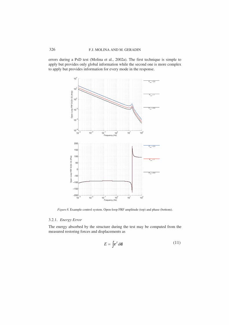
F.J. MOLINA AND M. GERADIN
errors during a PsD test (Molina et al., 2002a). The first technique is simple to apply but provides only global information while the second one is more complex to apply but provides information for every mode in the response.
Pcon
= 2.5
Pcon
= 1
Pcon
= 0.5
10−3 10
−210
−110
0 101
102
10−6
10−4
10−2
100
102
104
Frequency (Hz)
Ope
n−Lo
op F
RF
D/(
Dr−
D)
(Am
p)
Pcon
= 2.5
Pcon
= 1
Pcon
= 0.5
10−3
10−2
10−1
100
101
102
−200
−150
−100
−50
0
50
100
150
200
Frequency (Hz)
Ope
n−Lo
op F
RF
D/(
Dr−
D)
(Pha
)
Figure 8. Example control system. Open-loop FRF amplitude (top) and phase (bottom).
3.2.1. Energy Error
The energy absorbed by the structure during the test may be computed from the measured restoring forces and displacements as
dr dE T (11)
326

EARTHQUAKE ENGINEERING EXPERIMENTS AT JRC-ELSA
In can also be estimated in terms of the variables seen by the integration algorithm, i.e. the measured restoring forces and reference displacements,
rdr dE Tr
(12)
Now, let us define the energy error as the difference between (11) and (12), which is also the work done by the restoring forces on the displacement error:
rddrdrdr rr ddddEEE TTTTr )( (13)
By comparing this energy error with the total energy of Eq (11), a global upper estimate of the damping error effect due to the control error is obtained (Thewalt and Roman, 1994, Molina et al., 2002). When applying this variable as a global indicator, our experience is that in general, for an acceptable quality in the test results, the energy error should not exceed, say, a 5% of the total absorbed energy at any moment. Once the testing parameters such as the controller gains and the testing speed have been settled, a short-duration very-low-intensity test should be done to check this criterion. If the criterion is satisfied for that preliminary test in the linear range of the structure, the quality of the results should in general improve for larger amplitudes because, with the degradation of the structure, the damping ratio should grow while the eigenfrequency decreases and, as a consequence, the damping error introduced by the control should also decrease (look for example at Eq. 9 and Figure 6).
3.2.2. Spatial Model
This technique is based on the identification of a linear model of the structure using a narrow time window of the experimental response. The identified parameters are then transformed into frequency and damping characteristics that give very useful information regarding the quality of the performed test. By gaining experience in the application of this identification, it is possible to have better knowledge of what the feasibility and the accuracy of the experiment can be depending on the type of structure and the applied PsD testing set-up.
For the identification of the eigenmodes of the structure from the results of a PsD test, in fact, two different time-invariant linear models have been proposed that can be used working in the time domain (Molina et al., 1999a). The advantage of working in the time domain is in the easiness to automate the identification process. The simplest and most robust model is a spatial one that is going to be described here. Within this model, it is assumed that the measured
327

F.J. MOLINA AND M. GERADIN
restoring forces and the corresponding displacements and velocities are linked, for every discrete time n , in the form
)()()( nnn CvKdr (14)
where ( )nr , ( )nd and ( )nv result from the test. Of course, the linear stiffness and viscous damping of this model must be interpreted as an approximation to the real non-linear hysteretic behaviour. For identification purpose, the model can be rewritten in the form
)()()( nnn T
T
T
T
TT roCK
1vd (15)
where a constant force offset term o has also been added and 1 is a column of ones. Here, if DoFn is the number of DoFs in the structure, K , C and ocontain 22 DoF DoFn n unknowns and the number of available equations is
DoFN n , so that, the minimum required number of discrete-time data sets is
12 DoFnN (16)
Once K , C and o have been estimated by a least squares solution, the complex eigenfrequencies and mode shapes can be obtained by solving the generalised eigenvalue problem (Maia and Silva, 1997)
sC M K 0
0M 0 0 M (17)
where M is the theoretical mass matrix. The complex conjugate eigenvalues can be expressed in the form
)1(, 2*nnnnn jss (18)
where n is the natural frequency and n the damping ratio. The corresponding mode shape is also given by the first DoFn rows of the associated eigenvector n .
328

EARTHQUAKE ENGINEERING EXPERIMENTS AT JRC-ELSA
Since this model assumes an invariant system, at any selected time instant, an identification may be done based on a data time window, of duration roughly equal to the period of the first mode, centred around that instant. The adopted time window has to be narrow enough so that the system does not change too much inside of it, but, at the same time, it has to contain enough data to allow the compensation of different existing data noises and nonlinearities. The selection of the most appropriate window length is done by trial and error. It is usually possible to estimate the eigenfrequencies and damping ratios of all the modes at any time instant.
In order to use the method for the assessment of the error on the PsD response, the identification process may be repeated for two sets of variables entering in the model of Eq (14)), that is,
First set: measured forces, measured displacements and derived velocities,
Second set: measured forces, reference displacements and derived velocities.
The first set of variables takes into account the synchronous measured forces and displacements on the specimen without any influence from the control errors so that the identified frequencies and damping from this set are considered the real ones. For the second set, the considered forces and displacements are the ones entering in the PsD equation and the eigenfrequencies and damping linking them are the ones that explain the test response. For every frequency or damping ratio of the structure, the difference between the identified value with both sets of data is considered as the error introduced by the control system. As for the energy error criterion application, it is recommended to set the testing parameters so that, for the small-amplitude checking test, the damping error for every mode is kept under a 5% of the total damping of that mode. Looking at Eq. (9) and Figure 6, it is easy to understand that the higher modes with low damping use to be the most conditioning ones for the PsD test quality (Molina et al., 2000). Some results of the application of this estimation technique will be shown in the following section for a particular performed test within the SPEAR project.
As a different application, during the large-intensity tests, the identified response parameters may also be used to predict the response for a short time lapse. This is useful for piloting the test and may help taking the decision of stopping it before a dangerous configuration is attained by the structure.
4. Bidirectional PsD Testing (SPEAR Project)
For PsD testing of building specimens in one direction without torsion, normally two hydraulic actuators acting in that direction are used per floor. A first bidirectional PsD test was successfully performed on a real-size frame in 1997 at
329

F.J. MOLINA AND M. GERADIN
ELSA by using two actuators acting on each direction for everyone of its three floors (Molina et al., 1999b). At every integration step of the equation of motion, the developed procedure included, firstly, the transformation of measured restoring forces from the four actuator coordinates to the three DoFs of every floor, secondly, the finite-difference prediction of the new displacement and, thirdly, its transformation into actuator displacements. Those new target displacements were then imposed to the structure.
The testing technique described in this section has been applied for obtaining the experimental bidirectional response of a reinforced concrete (RC) three-storey building within the SPEAR project. The SPEAR project (Seismic Performance Assessment and Rehabilitation) focused on existing buildings because of the current economic and social relevance of their seismic performance. The experimental campaign on this structure consisted of rounds of seismic tests on the original structure and on two retrofitted configurations. This section describes essentially the testing technique and the corresponding experimental set-up; more information about the project itself, the structural characteristics of the specimen and the test results has been given by Mola et al. (2004) and Negro and Mola (2005).
4.1. TESTING TECHNIQUE
This subsection covers many of the aspects of the applied PsD testing technique, starting with the formulated general equation of motion (including three DoFs per floor) and time integration algorithm, and following with the specific force and displacements coordinate transformations needed for the adopted control system and strategy. Details on the implemented step-by-step testing procedure and on testing hardware and software characteristics are also given.
4.1.1. Equation of Motion
The mass of the building is assumed to be concentrated at the rigid floors, so that the equation of motion of every floor in the horizontal plane takes the form
gma r mja (19)
where the floor mass matrix
330

EARTHQUAKE ENGINEERING EXPERIMENTS AT JRC-ELSA
m 0 0
0 m 0
0 0 I
m(20)
is expressed in terms of the floor mass m and moment of inertia I at the Centre of Mass (CM), and
2 2
2 2x y x y
d da a a d d d
dt dt
T Ta d
(21)
is the vector of relative accelerations, which is the second derivative with respect to time of the floor relative displacements xd , yd and rotation d at the CM (Figure 9). Since the laboratory time will not be used at all within this section, the classical symbol t will refer to prototype time.
The vector of conjugated generalised restoring forces
x yr r rT
r (22)
Figure 9. Floor axis, actuators and displacement transducers.
331
F.J. MOLINA AND M. GERADIN
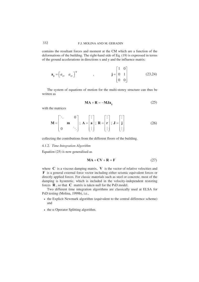
contains the resultant forces and moment at the CM which are a function of the deformations of the building. The right-hand side of Eq. (19) is expressed in terms of the ground accelerations in directions x and y and the influence matrix:
gx gya aT
ga ,
1 0
0 1
0 0
j (23,24)
The system of equations of motion for the multi-storey structure can thus be written as
gMA R MJa (25)
with the matrices
0
; ; ;
0
M m A a R r J j (26)
collecting the contributions from the different floors of the building.
4.1.2. Time Integration Algorithm
Equation (25) is now generalised as
MA CV R F (27)
where C is a viscous damping matrix, V is the vector of relative velocities and F is a general external force vector including either seismic equivalent forces or directly applied forces. For classic materials such as steel or concrete, most of the damping is hysteretic, which is included in the velocity-independent restoring forces R , so that C matrix is taken null for the PsD model.
Two different time integration algorithms are classically used at ELSA for PsD testing (Molina, 1999b), i.e.,
the Explicit Newmark algorithm (equivalent to the central difference scheme) and
the Operator Splitting algorithm.
332

EARTHQUAKE ENGINEERING EXPERIMENTS AT JRC-ELSA
The second method requires and estimation of the stiffness matrix of the structure which may affect the results if not properly chosen and updated. For this reason, the Explicit Newmark algorithm is preferred whenever a time increment
t may be chosen such that the algorithm is stable and the test duration is feasible. The stability is guaranteed when
mint T (28)
where minT is the minimum period of the structure. The Explicit Newmark algorithm was adopted for the SPEAR test. It may be
written in the form
1 1 1 1
21 1
1 1
1
2
1
n n n n
n n n n n
n n n n
t t
t
MA CV R F
D D V A A
V V A A (29)
with the specific parameter values
10;
2(30)
Contrarily to an integration based on a finite element model of the structure, in a PsD test, the restoring forces at every time step are not computed. They are directly measured on the physical model after imposition of the corresponding displacements:
)( 11 nn DRR (31)
Starting from known initial values 1 1 1, ,D V A , at time step =1 ( =0)n t , the successive computation stages of the method at every time step are:
Stage 1) Compute at instant 1n the values of displacements 1nD using Eq. (29).
Stage 2) Impose to the structure the new displacement 1nD and measure the associated restoring force of Eq. (31).
333

F.J. MOLINA AND M. GERADIN
Stage 3) Compute the acceleration at new time 1n from the equilibrium equation
1
1 1 12 2n n n n nt tA M C F R C V A (32)
Stage 4) Increment the step counter +1n n and go back to stage 1 until the final time is reached.
4.1.3. Kinematic Transformation from Generalised to Transducer Displacements
At every step of the PsD test, the computed generalised displacement of the floor is imposed through the actuators with feedback on the displacement transducers. Thus, in order to determine the target displacements at transducer level, a geometric transformation is needed. A minimum number of 3 high-resolution linear displacement transducers are attached to each floor for control purpose.
As shown in Figure 10, each control displacement transducer consists of a slider G1-G2 on which a body M translates and gives a measure of its relative position on the slider. The slider is attached to a fixed reference frame while the mobile body M is connected to the measuring point D on the structure through a pin-jointed rod.
x
y
CM
O
SC
DST ˆ
SD
D
x
yDS q
G1
D’
D
G2M
eG
lD
For every floor, starting from a known set of generalised displacements d(21), the position of the floor CM is updated as
dSS 0CC
(33)
Figure 10. Control displacement transducer.
334

EARTHQUAKE ENGINEERING EXPERIMENTS AT JRC-ELSA
whereT
CS CCC yx (34)
are its global coordinates and 0CS are their reference value for zero displacement.
Then, the position of the measuring point D is likewise updated as
DD STSCˆ
C
C
D
D
y
x
y
x (35)
where
D
D
y
x
ˆ
ˆˆDS
(36)
are the coordinates of point D in a reference system local to the floor, centred at its CM, and
CC
CC
cossin
sincosC
T (37)
is a rotation matrix. Assuming an infinitely rigid floor, the local coordinates of Eq. (36) are constant.
In order to express the position of body M (Figure 10) of the transducer along its slider 1 2G G , the relative position of the measuring point D with respect to the slider origin 1G is computed as
G1DD SSS DG1
~ (38)
and the projection of vector of Eq. (38) along the slider is obtained as
GD eS TDGq~
1(39)
where Ge is the constant unit vector defined in the direction of positive measurement along the slider.
The position of body M along the slider is then given by
2211 )sign( qDDlqqDMDGMGS DD
(40)
335

F.J. MOLINA AND M. GERADIN
being Dl the constant length of the rod. Finally, the corresponding measure at the transducer is
0DDD SSd (41)
where0
DS is a prescribed reference position.
The actual displacements and rotation at the CM will differ from the desired ones and this is due to geometry and control errors as well as to the flexibility of the floor. In order to get an estimate of the actual generalised displacements, the measures given by all the control displacement transducers may be exploited. Since the obtained relations between generalised and transducer displacements are non-linear and cannot easily be inverted in closed form, the solution is achieved through a Newton-Raphson iteration procedure starting from a first estimate of the generalised displacements, e.g.,
0dEST (42)
The non-linear equations giving the associated transducer displacements Ddare applied by substituting d by ESTd into Eq. (33) and applying Eqs. (35) to (41)
ESTEST ddd DD(43)
The difference between this estimate and the measured transducer displacements Dd is used to provide an new estimate of the generalised displacements
ESTESTEST dddJd DD1 (44)
where J is the Jacobian matrix
ESTd
D
ddJ
(45)
computed at ESTd .
4.1.4. Kinematic Transformation from Measured to Generalised Displacements
336

EARTHQUAKE ENGINEERING EXPERIMENTS AT JRC-ELSA
Taking into account Eq. (40), every single row of J can be obtained as
D Dd d GD MD q
MD
T TTD D G DG
D D D
S S e Sed S d S S d
(46)
If the number of control transducers on the floor exceeds 3, Eq. (25) must be solved in a least squares sense, in which case the inverse of J in Eq. (44) is replaced by the pseudo-inverse
psinv1T T(J) J J J (47)
The steps of Eqs. (43)-(44) are iteratively repeated until a specified tolerance is reached.
4.1.5. Static Transformation from Actuator to Generalised Forces
In a PsD test, the restoring forces are experimentally obtained from the specimen. Once the prescribed displacements are imposed, the acting axial force at every actuator is measured by its load cell. However, in order to express these forces as resultant generalised forces at the CM of the floor, a static transformation is needed. Since the ends of the actuator are pin-jointed, it is assumed that it acts with a purely linear force along the line PR (Figure 11) connecting the ends of the actuator. Starting from the load-cell measure Pr of this force and assuming that the current position of the floor CM is known, the global position of the loading point P is obtained as
PP STSC
ˆC
C
P
P
y
x
y
x (48)
whereC
T is given by Eq. (37). Similarly to Eq. (36), ˆPS contains the
coordinates of point P in the local reference system to the floor. Then, the global components of the piston force are computed as
PP ep Pr (49)
337

F.J. MOLINA AND M. GERADIN
where Pe is a unit vector in the direction of PR . The floor generalised restoring forces of Eq. (22) are obtained by summing up the effects of all pistons acting on the floor
PPPpTr (50)
where
PP xy
1
0
0
1
PT (51)
4.1.6. Optimal Distribution of Piston Loads
When using a number of actuators larger than the number of DoFs at a floor, it is convenient to maintain an acceptable distribution of loads among all the pistons. This can be done by implementing an algorithm capable of optimising the distribution of piston loads for a known set of generalised floor loads. Even distribution of forces is also desirable because it leads to a better approximation of the distributed inertial forces of a real dynamic event.
x
y
y
CM
r
ry
rx
REACTION WALL
x
PS
rP
CS
PST ˆ
P
R
To this purpose, the piston forces will be defined as ‘optimal’ if statically equivalent to the specified generalised loads and while minimising a penalty function that becomes infinite when any piston force reaches its working limit. The adopted expression for the penalty function is
Figure 11. Force applied by the actuator.
338

EARTHQUAKE ENGINEERING EXPERIMENTS AT JRC-ELSA
P PP rMf 22
1)( Pr (52)
where PM is the working limit of the absolute value of the piston load Pr .Clearly, minimising the function of Eq. (52) will guarantee that all piston loads are kept far from their limit. Using Eqs. (49) - (50), the conditions of static equivalence of the piston loads with the known set of generalised loads give a constraint on the minimisation problem which can be written in the vector form
PPPP r 0reTrg P )( (53)
where r is the known set of generalised forces of Eq. (22). The constrained minimisation problem is then
0rgr
P
P
)(
)( minimumf (54)
By introducing a set of Lagrange multipliers associated to the constraint equations, it can be restated in unconstrained form, leading now to the stationarity condition
0xh (55)
of the augmented functional
rgrx PT
P )()()( fh (56)
The solution vector r
x P (57)
contains as unknowns the piston loads and Lagrange multipliers
T321
(58)
The system of Eq. (55) may also be written as
0A(x) (59)
339
F.J. MOLINA AND M. GERADIN
where
rRr
RA(x)
P
T222
2
PP
P
rM
r
(60)
and, from Eq. (53),
PPeTR (61)
Since Eqs. (59) are nonlinear, their solution may be obtained through Newton-Raphson iteration in a similar way as done for obtaining the generalised displacements. Thus, starting from an initial estimate ESTx of the unknowns, each iteration would consist in computing
ESTEST xAB (62)
from Eq. (60) and updating the estimated optimum parameters by doing
ESTEST1EST xB0Jx (63)
where the Jacobian matrix is now
0R
R
xAJ
T
xEST
0
620
322
22
PP
PP
rM
rM
(64)
340
EARTHQUAKE ENGINEERING EXPERIMENTS AT JRC-ELSA
4.1.7. Piston Internal Displacements
A further step for indirectly imposing a desired load at the redundant pistons, mentioned at the preceding subsection, is the calculation of the displacement of their internal transducer. This is because using the internal displacement as feedback variable leads to a stable control of the redundant actuators.
Every actuator has an internal displacement transducer measuring the displacement Pd which represents the excursion of the piston. This displacement is a function of the floor generalised displacements d . Once the position of the CM in Eq. (34) is known and the position PS of the point P (Figure 11) of attachment of the piston to the floor calculated by Eq. (48), the current length of the piston is computed as
PRPPRP SSSS TPS (65)
and the internal displacement is
PPP SSd 0 (66)
where0
PS is the reference length. A positive value of Pd means a reduction of the actuator length.
4.1.8. Marching Procedure
The time integration of the 3-DoF-per-floor model has then be achieved following an experimental step-by-step procedure. The algorithm starts from known initial values 1 1 1, ,D V A and the operations are organised in the following stages:
Stage 0) Let 0n .
Stage 1) Transform the generalised displacements into target displacements
Dd at the control transducers computed from Eq. (41):
1nTARGET
1n Ddd DD(67)
Stage 2) Send these target displacements of Eq. (67) to the controllers which impose them to the specimen.
Stage 4) Measure the attained displacements 1
MEAS
nDd and restoring loads
1nPr at the controllers, Pr being the forces applied by the pistons.
341

F.J. MOLINA AND M. GERADIN
Stage 5) From the measured control displacements, by using the iterative least-squares solution of Eq. (44), estimate the generalised displacements on each floor
1 1
MEASMEASn nDD D d (68)
Stage 6) From the measured piston forces, by using the transformation Eq. (50), compute the new generalised restoring forces
1 11, MEAS
n nnPR R r D (69)
Stage 7) If 1n , by using Eq. (32), compute the new accelerations
1 1 1 1, , ,n n n n n nA A F R V A (70)
Stage 3) Let 1n n .
Stage 8) Predict the generalised displacement at the next time increment by using the finite-difference approximation Eq. (29) of the integration algorithm:
1 1( , , )n n n n nD D D V A (71)
Stage 9) Go back to stage 1) until reaching the final time.
4.1.9. Control Strategy
Let us assume that PID controllers are used and that, at each floor, three actuators are controlled using as feedback the corresponding displacement transducer on the structure. In that case, there are, in principle, three options in the choice of the feedback transducer to control the remaining redundant actuators:
a) the aligned displacement transducer on the structure (as for the other three actuators),
b) the actuator load cell force or
c) the actuator internal displacement transducer.
The first option is not practicable in general because the control system becomes unstable even for very low controller gains due to the high stiffness of the floor slab relatively to the stiffness of the pistons. The second option may lead to a stable control system, but, usually, force control strategies result in poor accuracy. It could be acceptable for a cyclic test, but not for a PsD test in which
342

EARTHQUAKE ENGINEERING EXPERIMENTS AT JRC-ELSA
relatively small control errors may result in a large distortion of the integrated response as commented in the previous sections.
The third option may give an accurate and stable control system since it is a displacement control strategy, as in the first option, but associated to a transducer which sees a more flexible subsystem. In fact, the displacements measured by the internal transducer of the actuator are considerably larger than those coming from the flexibility of the floor slabs since they comprise also the deformation of the reaction wall and actuator attachments as well as a part of the floor slab deformation. Thus, the actuator internal transducers have been adopted as feedbacks for the redundant pistons. In practice, the computed target for the redundant pistons is slightly adjusted at every integration step in order to control the distribution of loads on the floor at the same time. So, instead of using
Eq. (67), their target is computed as
1nP1nPTARGET
1nP ddd D (72)
where the first term on the right-hand side is the theoretical elongation of the piston in Eq. (66) and the second one is a correction introduced in order to modify the force. The latter is updated at every time step in the cumulative form
1
OPTIMUM MEASUREDP P n
P Pn n
P
r rd d
K
(73)
where the term added to the previous correction is the difference between the computed optimum force of Eq. (63) of the piston and the measured one at the former step, divided by a stiffness parameter PK empirically selected. In general terms, the smaller the parameter, the faster is the convergence of the force to the optimum value. However, using a too small value may result in instability, which would make the force to oscillate out of control in very few steps.
4.2. HARDWARE SET-UP
The servo-control units used for this experiment were MOOG actuators with 0.5 m stroke and load capacity of 0.5 MN. The control displacement transducers
on the structure were optical HEIDENHAIN sensors with a stroke of 0.5 m and 2 m of resolution. Every actuator was equipped with a load cell, a TEMPOSONICS internal displacement transducer and a PID controller based on a MSM486DX CPU executing the digital control loop at a sampling period of2 ms. The four controllers for the four pistons of each floor were governed by a
343

F.J. MOLINA AND M. GERADIN
powerful master CPU which is able to transmit and receive the controllers signals at real time (every 2 ms) through a high-speed communication channel based on dual port RAM boards. The three master units for the three floors had a common clock signal for the 2 ms interrupt. Those master controller units are programmed in C and have been designed to be able to apply complex algorithms in which the signals of several actuators are combined in real time. The sampling period of 2 ms has shown to be fast enough for stable digital control of structural specimens by hydraulic jacks but could be too short for cases in which the computations for those algorithms may become cumbersome. This hardware may permit the implementation of a PsD test with three DoFs per floor on a real time continuous basis only if the algorithm computation for each floor at every step can be performed in less than 2 ms.
For the classical implementation of the PsD method (subsection 2.1) adopted for this test, all master units were connected to a Windows workstation by means of ETHERNET. On such workstation, an application developed at ELSA and called STEPTEST executed the PsD test. This application is written in interpreted language (MATLAB) and implements the described model and marching procedure with interactive capabilities for monitoring and controlling the test (Figure 12).
4.3. TESTS PERFORMED IN THE FRAMEWORK OF SPEAR PROJECT
Within the SPEAR project, a full-size RC building model has been tested at ELSA. The mock-up is representative of non-seismic construction of the 60-70’s in southern European countries, irregularities in plan and detailing included (Negro and Mola, 2005). The structure is a simplification of an actual Greek three-storey building and was designed for gravity loads alone using the Greek design code applied from 1954 to 1995. As seen in Figure 13, it has a doubly
unsymmetric plan configuration, but it is regular in elevation. It is made of three 2-bay frames spanning from 3 to 6 m in each direction with a storey height of 3 m.
For practical reasons, the specimen was built outside of the laboratory, starting from a thick RC base slab on which the ground columns were anchored. Afterwards, the base was rolled over PVC rolls (Figure 15) in order to transport the built specimen up to its final position on the strong floor of the laboratory, where it was clamped with post-tensioning bars.
As shown in Figure 9, four actuators with four associated control displacement transducers were used for the bidirectional testing of the structure. In principle, these actuators were connected to the floor in positions not too close to the structural joints. Additional RC stiffeners were created in the floor slabs
344

EARTHQUAKE ENGINEERING EXPERIMENTS AT JRC-ELSA
(Figure 15) in order to properly distribute the local force applied by the pistons. The clamping of the piston attachments included post-tensioning bars. The piston bodies were supported by the reaction wall or by a supplementary reaction structure while the control displacement transducers were fixed on unloaded reference frames (Figure 9).
Apart from the load cells and control displacement transducers, additional instrumentation was installed on the specimen. Damage was expected mostly on top and bottom of the columns of the first two stories. Accordingly, clinometers were installed on up to three levels of each column. Additionally, some potentiometer extensometers were also installed on some localised areas. For the first time at ELSA, photogrammetry techniques were applied to a bidirectional test and, at two locations, a couple of cameras were used in order to record stereo images and estimate the bidimensional displacements of marked targets.
The CM, total mass and moment of inertia for the PsD equations were obtained from the theoretical mass distribution for the seismic assessment of the building according to Eurocode 8. Since the corresponding weight of the model was lower, additional water containers (Figure 16) were set on the floors of the specimen in the laboratory in order to have realistic gravity loads at the members. The input signals for the test were semi-artificial records modulated consistently with Eurocode 8. After some preliminary small tests to verify the testing system and tune the control parameters, two big PsD tests were performed for peak ground acceleration of up to 0.20 g, on the original specimen, and 0.30 g on the two retrofitted configurations. For each test, the intensity of the excitation was equal in the horizontal x and y components but the history of ground acceleration was different.
Details on the obtained response and damage at the different configurations are given by Negro and Mola (2005). During the different tests, the obtained maximum displacements at the third floor were in the order of 200 mm in the “x” (weak) direction, 150 mm in the “y” direction and 23 mrad of torsion. This level of torsion was higher than the predicted one using regulated methods.
The tests were performed with very low experimental error. For example, the errors produced at the controller loops were always lower than 0.1 mm and those estimated in the generalised displacement at the CM were lower than 0.3 mm. The latter are mostly due to the existing flexibility of the floors since three structural displacements were used for the control while all four of them entered in the estimation of the generalised displacement. An overall manner to assess the quality of a PsD test in relation to the existing control errors is through the computation of the energy of error (as we have commented in subsection 3.2.1), which amounted some 50 J, in comparison to the total absorbed energy in the structure, which was around 130 kJ for the second test for example. A way to look
345

F.J. MOLINA AND M. GERADIN
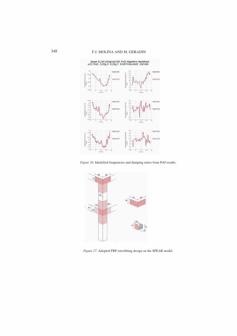
in more detail at the effects of the control errors on each mode consists of the identification of the eigenfrequency and damping from the measured forces and from the measured and reference displacements (see subsection 3.2.2). For example, for the 0.20 g test on the original specimen, the identified values for the first three modes at different time instants are shown in Figure 17. The results for the other estimated six modes are not much worse. The conclusion is that the control errors verified during the test have not affected at all these clue parameters for the response of the structure.
Figure 12. Controller set-up for the PsD tests.
After the testing campaign on the original model, a second round of tests was run on the first retrofitted configuration which tempted to increase the poor ductility capacity of the original columns and joints by means of the application
Figure 13. Plan and 3D views of the SPEAR RC building specimen.
346

EARTHQUAKE ENGINEERING EXPERIMENTS AT JRC-ELSA
of uniaxial and multiaxial glass-fibre wraps (Figure 18). For this configuration, the introduced ground acceleration level arrived up to 0.30g which produced 200mm displacement in the X direction and 120mm in the Y direction. After that, the glass fibre was removed and an alternative retrofitting intervention was introduced by means of RC-jacketing of two of the columns at all the levels. This second kind of intervention was focused to reduce the eccentricity between the CM and the centre of strength in the X and Y direction, without regarding the ductility capacity of the remaining members. For this second retrofitted configuration, the 0.30g earthquake produced displacements of 160mm in the X direction and 130mm in the Y direction.
Figure 14. Transportation of the building specimen inside of ELSA.
Figure 15. View of the structure ready for the PsD tests.
347
F.J. MOLINA AND M. GERADIN
Figure 16. Identified frequencies and damping ratios from PsD results.
Figure 17. Adopted FRP retrofitting design on the SPEAR model.
348

EARTHQUAKE ENGINEERING EXPERIMENTS AT JRC-ELSA
5. Conclusions
Some of the main capabilities and achievements in structural testing at the ELSA laboratory have been summarised in this chapter. As a complement to other laboratories in Europe, ELSA has specialised itself in tests on large-size models and with sophisticated computer-controlled load-application conditions. Internationally recognized pioneering steps have been achieved for the development of the PsD testing method and its full-scale implementation. The ELSA contribution includes also some cases of real dynamic tests of active and semi-active control systems as well as vibration monitoring.
As a difference with respect to a shaking-table test, the control and measuring errors in a PsD test can be very low thanks to the low speed of execution. However, as has been shown in this chapter, even small time delays at the control may still significantly reduce the apparent response damping of the structure. Assessment methods that have been proposed give an on-line quantitative measure of the effect of the existing errors. They represent useful tools for controlling those effects and taking decisions in order to improve the quality of a PsD test. In the case of unacceptable distortion of the response, some parameters, such as the testing speed or the controller gains, may be changed during the test. Such parameter tuning is mainly performed during the preliminary small-intensity tests in order to assure the required accuracy.
In the framework of the activity of the SPEAR research project, three rounds of bidirectional PsD tests were carried out on a full-scale three-storey plan-wise irregular RC frame structure. The applied PsD technique considers three DoF per floor and includes rigorous geometrically non-linear transformation of coordinates for the actuator forces and displacements transducers attached to the floors. It also allows using more than three pistons and displacements transducers per floor, in which case it guarantees and even distribution of piston forces. The performed tests within the SPEAR project have been quite successful from the point of view of verified experimental error. The applied methodology showed to be quite appropriate for large-displacement bidirectional testing of full scale specimens. The results of these tests are of high relevance for understanding the torsional response of unsymmetric buildings.
Acknowledgements
Many members of the ELSA staff as well as project partners have provided significant contribution to the success of the activities described in this chapter. The authors gratefully acknowledge their contribution. Project SPEAR was funded by the EC under the “Competi tive and Sustainable Growth” Programme,
349

F.J. MOLINA AND M. GERADIN
Contract N. G6RD-2001-00525 and the access to the experimental facility took place by means of the EC contract ECOLEADER N. HPRI-1999-00059.
REFERENCES
De Luca, A., Mele, E., Molina, F. J., Verzeletti, G., Pinto, A. V., 2001, Base isolation for retrofitting historic buildings: evaluation of seismic performance through experimental investigation, Earthquake Engineering & Structural Dynamics, 30: 1125-1145.
Donea J., Magonette G., Negro P., Pegon P., Pinto A., 1996, Verzeletti, G. Pseudodynamic capabilities of the ELSA laboratory for earthquake testing of large structures. EarthquakeSpectra, 12:163-180.
Magonette, G., Pegon, P., Molina, F. J., Buchet, Ph., 1998, Development of fast continuous substructuring tests, Proceedings of the 2nd World Conference on Structural Control.
Magonette, G., F. Marazzi, H. Försterling, 2003, Active control of cable-stayed bridges: large scale mock-up experimental analysis, ISEC-02 - Second International Structural Engineering and Construction Conference, Rome.
Maia, N. M. M. and Silva, J. M. M. (editors), 1997, Theoretical and Experimental Modal Analysis,Research Studies Press, John Wiley.
Mola, E., Negro, P., Pinto, A. V., 2004, Evaluation of current approaches to the analysis and design of multi-storey torsionally unbalanced frames, Proceedings of the 13th World Conference on Earthquake Engineering, Vancouver, Paper N. 3304.
Molina, F. J., Pegon, P. and Verzeletti, G. 1999a, Time-domain identification from seismic pseudodynamic test results on civil engineering specimens, 2nd International Conference on Identification in Engineering Systems, University of Wales Swansea.
Molina, F. J., Verzeletti, G., Magonette, G., Buchet, Ph., Geradin, M., 1999b, Bi-directional pseudodynamic test of a full-size three-storey building, Earthquake Engineering & Structural Dynamics, 28: 1541-1566.
Molina, F. J., Gonzalez, M. P., Pegon, P., Varum H. and Pinto, A., 2000. Frequency and Damping Evolution During Experimental Seismic Response of Civil Engineering Structures. COST F3 Conference on System Identification & Structural Health Monitoring.
Molina, F. J., Magonette, G., Pegon, P., 2002a, Assessment of systematic experimental errors in pseudodynamic tests, Proc. of 12th European Conference on Earthquake Engineering, Elsevier Science , Paper 525.
Molina F. J., Verzeletti, G., Magonette, G., Buchet, Ph., Renda, V., Geradin, M., Parducci, A, Mezzi, M, Pacchiarotti, A, Federici, L., Mascelloni, S., 2002b, Pseudodynamic tests on rubber base isolators with numerical substructuring of the superstructure and strain-rate effect compensation, Earthquake Engineering & Structural Dynamics, 31: 1563-1582.
Molina, F. J., S. Sorace, G. Terenzi, G. Magonette, B. Viaccoz, 2004, Seismic tests on reinforced concrete and steel frames retrofitted with dissipative braces, Earthquake Engineering & Structural Dynamics, 33: 1373-1394.
Negro, P., Mola, E., 2005, Full scale PsD testing of the torsionally unbalanced SPEAR structure in the ‘as-built’ and retrofitted configurations, SPEAR Workshop, EC-JRC Ispra, Italy.
Network for Earthquake Engineering Simulation; http://www.nees.org. Phillips, C. L. and Harbor, R. D., 1999, Feedback Control Systems, Prentice Hall. Pinto, A. V., Pegon, P., Magonette, G., Tsionis, G., 2004, Pseudo-dynamic testing of bridges using
non-linear substructuring, Earthquake Engineering & Structural Dynamics, 33: 1125-1146.
350

EARTHQUAKE ENGINEERING EXPERIMENTS AT JRC-ELSA
Pinto, A. V., Pegon, P., Taucer, F., 2006, Shaking table facilities and testing for advancement of earthquake engineering: international cooperation, experiences, values, chances, FirstEuropean Conference on Earthquake Engineering and Seismology.
Shing, P. B., Mahin, S. A., 1987, Cumulative experimental errors in pseudo-dynamic tests, Earthquake Engineering & Structural Dynamics, 15: 409-424.
Takanashi, K., Nakashima, M., 1986, A State of the Art: Japanese Activities on on-Line Computer Test Control Method, Report of the Institute of Industrial Science, 32, 3, University of Tokyo.
Thewalt, C. and Roman, M., 1994, Performance Parameters for Pseudodynamic Tests, ASCEJournal of Struct. Eng., 120, 9.
351