extinction cascades and catastrophe in ancient food webs

BioOne sees sustainable scholarly publishing as an inherently collaborative enterprise connecting authors, nonprofit publishers, academic institutions, researchlibraries, and research funders in the common goal of maximizing access to critical research.

Extinction cascades and catastrophe in ancient food websAuthor(s): Peter D. RoopnarineSource: Paleobiology, 32(1):1-19. 2006.Published By: The Paleontological SocietyURL: http://www.bioone.org/doi/full/10.1666/05008.1

BioOne (www.bioone.org) is a nonprofit, online aggregation of core research in the biological, ecological, andenvironmental sciences. BioOne provides a sustainable online platform for over 170 journals and books publishedby nonprofit societies, associations, museums, institutions, and presses.

Your use of this PDF, the BioOne Web site, and all posted and associated content indicates your acceptance ofBioOne’s Terms of Use, available at www.bioone.org/page/terms_of_use.

Usage of BioOne content is strictly limited to personal, educational, and non-commercial use. Commercial inquiriesor rights and permissions requests should be directed to the individual publisher as copyright holder.

http://www.bioone.org/doi/full/10.1666/05008.1

http://www.bioone.org

http://www.bioone.org/page/terms_of_use

q 2006 The Paleontological Society. All rights reserved. 0094-8373/06/3201-0001/$1.00

Paleobiology, 32(1), 2006, pp. 1–19

Extinction cascades and catastrophe in ancient food webs

Peter D. Roopnarine

Abstract.—A model is developed to explore the potential responses of paleocommunities to dis-ruptions of primary production during times of mass extinction and ecological crisis. Disruptionsof primary production are expected to generate bottom-up cascades of secondary extinction, andthese are predictable given species richnesses, functional diversity, and trophic link distributions.If, however, consumers are permitted to compensate for the loss of trophic resources by increasingthe intensities of their remaining biotic interactions, top-down driven catastrophic increases of sec-ondary extinction emerge from the model. Both bottom-up and top-down effects are themselvescontrolled by the geometry of the food webs. The general Phanerozoic trends of increasing taxo-nomic and ecological diversities, as well as the varying strengths of biotic interactions, have led tofood webs of increasing complexity. The frequency of catastrophic secondary extinction increasesas food web complexity increases, but increased complexity also serves to dampen the magnitudeof the secondary extinctions. When intraguild competitive interactions are included in the model,competitively inferior taxa are observed to possess greater probabilities of survival if the guildsare embedded in simple subnetworks of the overall food web. The result is the emergence of post-extinction guilds dominated by those inferior taxa. These results are congruent with empirical ob-servations of ‘‘disaster taxa’’ dominance after some mass extinction events, and provide a mecha-nism for the reorganization of ecosystems that is observed after those events. The model makes thetestable prediction that dominance by disaster taxa, however, should be observed only when bot-tom-up disruptions have caused ecosystems to collapse catastrophically.

Peter D. Roopnarine. Department of Invertebrate Zoology and Geology, California Academy of Sciences,875 Howard St., San Francisco, California 94103. E-mail: [email protected]

Accepted: 29 July 2005

Introduction

Many of the species that became extinctduring intervals of mass extinction probablydid not succumb to the direct effects of abiotictriggers, but rather were victims of the resul-tant ecological crises and failing communities.The disruption of primary production is oftencited as a proximal cause of such crises (Ver-meij 1995; Martin 1996; Allmon 2001; Bentonand Twitchett 2003), because it is predicted tounleash avalanches of secondary extinctions athigher trophic levels (Borrvall et al. 2000; Ver-meij 2004). If an ecological community isviewed as an Eltonian pyramid of connectedtrophic levels (Elton 1927), then the effects ofan interruption of primary production aredriven from the ‘‘bottom up,’’ while the re-sponses of consumer activities are propagated‘‘top down.’’ Secondary extinction of a speciesmay occur as a direct result of bottom-up per-turbations to, or top-down impact from, otherspecies to which it is linked trophically or isotherwise dependent upon (Quince et al.2005). The simulation model presented here

combines bottom-up and top-down processesto provide a theoretical basis for understand-ing secondary extinctions in fossil communi-ties during times of mass extinction, withinthe context of community change during thePhanerozoic.

An ecological community may also beviewed as a directed energy transfer networkamong species, in which energy fixed by au-totrophic species is transferred with thermo-dynamically decreasing efficiency to otherspecies in the network (Lindeman 1942). Pri-mary production is interrupted by the extinc-tion of primary producers, their temporaryshutdown, or even their switch to a heterotro-phic lifestyle during stressful times. Ecologi-cal theory suggests that the effective reductionof primary production should have impactselsewhere in the community network (Vermeij2004), including the loss of consumer speciesas a response to the loss of autotrophic re-sources. Evidence supporting disruptions ofprimary production during episodes of ex-tinction includes anomalous excursions of car-bon stable isotope ratios at the end of the

2 PETER D. ROOPNARINE

Permian through Early Triassic (Knoll et al.1996; Benton and Twitchett 2003) and the endof the Cretaceous (Zachos et al. 1989), the lossof abundant or dominant photosynthetic spe-cies at the end of the Cretaceous (Sheehan andHansen 1986; Falkowski et al. 2004; Vajda andMcLoughlin 2004; Wilf and Johnson 2004),fungal spikes at the Cretaceous/Tertiaryboundary (Vajda and McLoughlin 2004) andpossibly the Permo-Triassic boundary (Eshetet al. 1995; Visscher et al. 1996; Benton andTwitchett 2003; but see Foster et al. 2002), andon a more regional scale, massive yet selectivespecies extinctions in marine ecosystems dur-ing the Pliocene in the tropical western Atlan-tic (Vermeij and Petuch 1986; Roopnarine1996; Anderson 2001; Allmon 2001; Todd et al.2002). Whether this type of bottom-up pertur-bation results in the extinction of consumers,and whether such secondary extinctions prop-agate as trickles or entire avalanches througha trophic network, might depend on severalparameters of the network. These include tax-onomic richness, functional or guild diversity,the pattern and relative strengths of trophiclinks between species, and the comparativespecies richnesses among guilds of similartrophic function but different composition (forexample, protistan phytoplankton and ben-thic macrophytes).

Very little can be known directly of themechanisms and pathways by which disrup-tions cause specific secondary extinctions inany particular ancient community, becausethe mechanisms must operate through com-plex trophic pathways and systems of some-times poorly known species diversities, inter-actions, and linkages. What we do know, how-ever, is that ancient ecosystems have changeddramatically over time with the evolution ofmajor new ecological roles (for example het-erotrophy) (Knoll and Bambach 2000), withthe variation of species diversity both in totaland within guilds (Bambach 1977; Sepkoski1981), with the secular increase in the ener-getics of biotic interactions (Vermeij 1987), andwith the evolution of species with increasedmetabolic rates and complexity (Bambach1993).

I propose that by modeling the generalfunctional structure of community trophic

systems, it is possible to compare the relativeeffects of disruptions of primary productivityamong communities of varying complexity.Based on this premise, the numerical modelpresented herein assesses the magnitude andextent of secondary extinction and extinctioncascades that were initiated in paleocommun-ities under varying levels of interruptions ofprimary production. Interruptions of produc-tivity in the model take the form of the deac-tivation of primary producers, as might be ex-pected under hypothesized physical condi-tions prevailing during episodes of mass ex-tinction. The model is based on the trophicnetwork (food web) representation of ecolog-ical communities (Elton 1927; May 1973). It fo-cuses specifically on the changing susceptibil-ity of paleoecosystems to secondary extinc-tion during the Phanerozoic as species rich-ness, ecological/functional diversity, andtrophic network complexity have varied. I alsoaccount for the fact that there are many detailsof community relationships that are unknow-able for fossil species and paleocommunities(Olszewski and Erwin 2004), and that thereare parameters of modern food web theory,such as trophic species and connectance (Wil-liams and Martinez 2000), that cannot bequantified and applied with measurable pre-cision in paleoecological contexts. The modelis therefore a probabilistic construct based onnecessary abstractions and estimates of com-munity ecological parameters.

Basic Model. The proposition that disrup-tions of primary production result in bottom-up cascades of secondary extinction was ex-amined by subjecting several hypothetical pa-leocommunities to press perturbations of pri-mary producers. Figure 1 shows a simplethree-node network with each node repre-senting a guild of species sharing the samesets of potential prey and predators. Thismeans that, for example, although the specificprey of two species are not known precisely,we can still identify the guilds to which theirprey most likely belonged. Each species with-in a consumer node possesses an in-degree, ornumber of incoming trophic links, or preyspecies. The in-degree of any particular spe-cies within a node is derived from a probabil-ity distribution P(r) that describes the in-de-

3EXTINCTION CASCADES

FIGURE 1. Simple three-node statistical trophic net-work. Each node represents a set of species that sharethe same sets of potential prey and predators. M, pri-mary producers; N1, primary consumers; N2, secondaryconsumers. Node designations also represent speciesrichness (see text formulae). Network on right desig-nates node N2 as a set of omnivorous species.

grees of all the node’s species. Suppose that aspecies’ survival in a trophic network reliessolely upon having at least one trophic (food)resource (ignoring top-down effects such aspredation). Then from Figure 1, if the level ofperturbation to M (that is, the disruption of pri-mary productivity) is v, then the probability ofsecondary extinction of any primary consumer(node N1) as a consequence of extinction of allits trophic resources in node M is

21M 2 r M v!(M 2 r )!1 1p(e z v) 5 5 (1)r1 1 21 2v 2 r v M!(v 2 r )!1 1

where P( z v) is the probability of extinctioner1

of a N1-taxon of in-degree r1 given that pri-mary producer shutdown is v species out ofM (see Appendix). The equation describes thenumber of ways in which it is possible for aconsumer with r prey to lose all those prey

when prey extinction is v $ r. The expected(average) number of secondary extinctions inN1, c1, is therefore

i5v

c 5 E(e z v) 5 [p(e z v)P(r )]NO1 r r 1 1N1 ii5rN1min

i5vN v! (M 2 r )!1 i5 p(r ) (2)O iM! (v 2 r )!i5r iN1min

where P(r1) is a probability density functiondescribing the in-degrees of taxa in node N1,and p(ri) is the probability of an N1-taxon hav-ing in-degree ri (Appendix). The equation im-plies that secondary extinction is a predictablefunction of primary producer extinction. Sec-ondary extinctions may propagate further tothe top-level node N2, where the expected lev-el of extinction, c2, given v and c1, is

c 5 E(e z v, c )2 r 1N2

i5c1N c ! (N 2 r )!2 1 1 i5 p(r ) (3)O iN ! (c 2 r )!i5r 511 1 iN2min

and p(ri) is the probability of an N2-taxon hav-ing in-degree ri. Increasing the functionalcomplexity of a food web is accommodatedsimply by extending the combinatorial basesof the formulae. For example, if N2 is insteada node of omnivores (Fig. 1B), expected ex-tinction becomes

c 5 E(e z v 1 c )2 r 1N2

i5(v1c )1N (v 2 c )! (N 1 N 2 r )!2 1 1 i5 p(r ).O i(M 1 N )! (v 1 c 2 r )!i5r1 1 iN2min

(4)

The summations on the right-hand side of theformulae have limits at v and c1 successivelybecause

0 , p(e z v, c ) # 1 if c $ r ,r 1 1 ii

and

p(e z v, c ) 5 0 if c , rr 1 1 ii

meaning that consumer species are immune tosecondary extinction if extinction in the preyguild is not greater than the consumers’ in-de-grees.

Extinction Thresholds. The realism of thebasic model can be increased in two ways, firstby recognizing a non-zero probability of ex-


tinction before a species or population loses allof its trophic resources, and second by incor-porating biotic interactions (Quince et al.2005), namely competitive interactions andtop-down consumer effects. Permitting a spe-cies’ populations to become extinct prior to theloss of all in-links (r) acknowledges that theloss of resources stresses population sustain-ability. For example, if the carrying capacity ofa population, K, is considered to be a functionof incoming energy and the state of the com-munity, then K and hence population size de-cline as the number of food sources decreases.Population size reaches a lower thresholdeventually where depensation (Allee effects)and stochastic factors make extinction inevi-table (Lande et al. 2003), even though r . 0.Approaching an extinction threshold cantherefore be described as changes in carryingcapacity resulting from the loss of trophic re-sources. If v . 0, then the probability of losinga fraction n links (resources) out of r is givenby the hypergeometric probability (compareto eq. 1)

21r M 2 r Mp(n z v) 5 (5)1 21 21 2n v 2 n v

and the expected value of n for any r and v issimply the hypergeometric mean value (rv)/M. Given a threshold T, extinction is thereforemost likely to occur when

K nnT $ [ T $ 1 2 (6)K rr

where Ki is the carrying capacity given i in-links. That is, when n 5 0, n/r 5 0, and ex-pected extinction is also zero (T always . n/r). The probability of secondary extinctionnow follows the rules

0 , p(e z v) # 1 if v $ r (1 2 T ),r ii

and

p(e z v) 5 0 if v , r (1 2 T ).r ii

Given the hypergeometric relationship be-tween n and v, extinction is now most likelywhen the expected relationship between theextinction threshold T and primary produc-tivity disruption v is

vT $ 1 2 (7)

M

(see Appendix).Top-Down Feedback and Competition. The

model is completed by incorporating top-down effects and competitive interactions.Top-down effects are generally mediated byconsumption (Hairston et al. 1960), and dif-ferent species within a guild or node maycompete for resources. Assuming that thecommunity is in equilibrium when v 5 0, thenthe amount of energy lost by a population topredation and denied to it by competitors is atleast balanced by incoming energy. The ener-gy being lost to predation is measured by theout-degree of the species, or number of out-links (consumers), and the strength or inten-sity of those links. Because the basic modelconsiders link strengths to be single-valuedand static, the loss of an in-link represents anet loss of energy to the consumer. Expandingthe model allows consumers to compensatefor lost in-links by increasing the strength ofremaining in-links, that is, increasing the in-tensity of predation. Without the ability tocompensate by altering the strength or inten-sity of in-links, consumer extinction would in-crease steadily to 100% as v → M. Compen-sation, however, is accomplished by increas-ing the intensity of remaining biotic interac-tions, and a consumer may maintain itsenergy budget by continuously increasing thestrength of remaining links. Such compensa-tion though has a negative impact on prey spe-cies, because it increases the rate at which preyspecies approach their effective extinctionthresholds. One possible result is the addi-tional extinction of prey species, followed byadditional extinction of any consumers whosubsequently lose all in-links, and further in-tensification of the link strengths of consum-ers who have lost some in-links. Thus, a pos-itive feedback loop is initiated between con-sumers and prey (Appendix).

Although the model considers a consumer’slink strengths to be single-valued, some em-pirical data and theoretical considerations ofthe distribution of interaction intensities ofmodern taxa suggest that the distribution of aspecies’ link strength may be skewed, with a


predominance of weak or intermediate linkstrengths (Paine 1992; Goldwasser andRoughgarden 1993; McCann et al. 1998). Linkstrength here, however, was measured as afraction of the consumer species’ in-degree ordietary diversity (1/r), with the initial pre-dation intensity on a prey species being

i5d 1S 5 (8)O

ri51 i

where d is the number of predators (out-de-gree of prey) and 1/ri is the link strength ofthe ith predator. All of a consumer’s links aretherefore of equal strength, though thisstrength varies among consumers as the num-ber of food sources (r) varies.

The effect of competitive interactions maybe modeled similarly by determining a spe-cies’ relative rank among its competitors (thatis, competitive rank normalized by the diver-sity of competitors). Extinction of a species’competitors makes more resources available,and would offset the subsequent increase inthe predation intensity by a predator commonto both the species and its extinct competitors.Combining energy lost to predation and com-petitors, the threshold for extinction may nowbe reformulated as

p(e) 5 1 when

1 S 2 S R 2 Rv 0 0 vT $ 1 2 1 (9)1 22 S R0 0

where Si is predation intensity and Ri is com-petitive rank within a guild when i 5 v. S0

and R0 are predation intensity and competi-tive rank respectively when v 5 0. The ex-tinction of competitors should serve to slow apopulation’s approach to its extinction thresh-old. Note that the combinatorial formulae re-lating v and secondary extinction are no lon-ger present. The above formula, however, is asimulation rule that ensures the interaction ofthe network parameters (diversities, link dis-tributions), T, S, and R (Appendix).

The model is parameter-rich, reflecting themultivariate character of food webs (de Ruiteret al. 2005). The parameters for any given sim-ulation comprise the input parameters ofguild diversities, the level of primary produc-er disruption (v), trophic link distribution co-

efficients (g), guild extinction thresholds (T),as well as variable but dependent parameters,namely link strengths (S) and competitiverank (R). The model is not deterministic, how-ever, because of the stochasticity involved inassembling individual food webs (see ‘‘Meth-ods’’), and several interesting and unexpectedphenomena emerge from the simulations (see‘‘Results and Discussion’’), notably top-downdriven extinctions caused by bottom-up per-turbations, catastrophic increases of second-ary extinction in response to incremental in-creases of primary producer disruption, andthe sometimes biased nonrandom survival oftaxa of low competitive ranks.

Methods

Analysis of the model proceeded by con-structing probabilistic paleocommunitieswith trophic connections, applying the for-mulae and rules described in the previous sec-tion, and simulating extinction by the randomremoval of links to primary producers. Com-puter simulations were used to evaluate themodel in lieu of alternative approaches (forexample, systems of differential equations;Appendix) mostly because the simulationspermit the collection of data on individualtaxa (see below), in addition to visualizationof the ensemble behavior of guilds and com-munities. The intuitive nature of computersimulations also make them more accessible toa broader audience.

Model Networks. Constructing probabilisticnetworks on the basis of known propertiesand distributions of existing trophic networks(Havens 1992; Martinez 1992; Montoya andSole 2002) allows us to explore paleo-trophicnetwork response to varying levels of primaryproducer perturbation and shutdown. Datathat are difficult to obtain both neontological-ly (Goldwasser and Roughgarden 1997) andpaleontologically, however, dictate to a largeextent the reconstruction of paleotrophic net-works. For example, no single stratigraphicsample, nor necessarily even a series of later-ally contemporaneous samples, can be consid-ered as the sole basis for network construction.The networks must be the result of regionallyintegrated sampling, which in turn measuresthe temporally and geographically stable


pools of species from which the componentsof local communities were assembled. Speciesinteractions are also frequently obscure(Leighton 2004). These interactions can onlybe inferred for fossil species, and even thoseinteractions that are inferred with great con-fidence, for example the direct evidence of pre-dation via skeletal scars or gut contents, arerepresentative of an essentially unknowableset of potential interactions among large num-bers of species. Interaction strengths are like-wise difficult to specify and are rarely consid-ered even in neoecological studies (Goldwas-ser and Roughgarden 1993). Finally, certainimportant food web components often pre-serve very poorly in the fossil record, for ex-ample skeletogeneous phytoplankton withskeletons that are highly soluble under certainconditions, benthic macrophytes with few orno hardparts, and top-level consumers withsmall population sizes and hence relativelylower fossilization rates. Although these datacannot always be obtained for fossil species,potential prey and predators can often beidentified by relying upon morphology, geo-graphic and sedimentological proximity, phy-logenetic affinity, and uniformitarian compar-ison to extant taxa. Species may therefore begrouped into guilds or nodes on the basis ofsimilar potential interactions. Links betweenspecies, and the properties of links (for ex-ample, interaction strengths), cannot be spec-ified as scalar quantities, but instead shouldbe based on distributions, which are in turnderived from reasonable inferences of organ-ismal and autecological data.

Hypothetical communities were thereforeconstructed on the basis of the simple three-node network model illustrated earlier, as wellas Bambach’s megaguild characterization ofCambrian, post-Cambrian Paleozoic, and Me-sozoic–Cenozoic marine communities (Bam-bach 1983) (Fig. 2), in turn derived from Sep-koski’s evolutionary faunas (Sepkoski 1984).These characterizations are distinguishedfrom each other by the increasing diversity ofmegaguilds during the Phanerozoic (Bam-bach 1983), as well as the increasing numberof trophic connections between megaguilds,and serve as a first approximation of com-munity changes in shallow marine commu-

nities during the Phanerozoic. Species rich-nesses were assigned to reflect the relative di-versity of higher taxa within megaguilds, butwere held approximately constant within tro-phic levels among the three networks (subse-quent analyses based on varying relative spe-cies richnesses produced results differing verylittle from the present results). The three-nodenetwork was assigned diversities of 1000 pri-mary producer species (M), 100 primary con-sumers (N1), and ten secondary consumers(N2), with secondary consumer species diver-sities being scaled and reduced overall by afactor of ten relative to total primary consum-er diversity. Node diversities were assigned tothe model megaguild paleocommunities asfollows: Cambrian, PS-100, ES-400, ED-300,EH-200, SIS-100, SID-200, PC-65, SIC-65; Pa-leozoic, PS-96, ES-640, ED-128, EH-160, SIS-128, SID-128, DID-32, PC-52, EC-52, SIC-26;Mesozoic, PS-81, PH-54, ES-513, ED-54, EH-135, SIS-162, SID-108, DIS-135, DID-54, PC-45,EC-45, SIC-36, DIC-9 (see Fig. 2 for an expla-nation of node designations). Primary pro-ducer diversity (or level of productivity) wasset at 2600 for each parameter set. Primaryconsumer species diversities were scaled andreduced overall by a factor of two relative tototal primary producer diversity, and diver-sity in each subsequent trophic level was re-duced as a factor of ten relative to the nextlowest trophic level. Deposit feeders werelinked directly to primary producers, becauseon the timescales considered here, as well asthe potentially short trophic distance betweenmany deposit feeders and primary production(Levinton 1996), the effects of primary pro-ducer extinction would not be expected to dif-fer greatly between primary herbivores anddeposit feeders.

The webs illustrated in Figure 2 are there-fore summary schematics, within which areembedded detailed species-level directed net-works. The connections of each network varyfrom one simulation to the next (described be-low) but conform to the specific distributionsdetermined by guild diversities and link dis-tributions.

Numerical Simulations. The in-degree (num-ber of incoming trophic links) of each specieswithin a node was drawn randomly from a


FIGURE 2. Hypothetical model marine food webs based on megaguild scheme. Each node represents a set of speciesof particular trophic habit, and arrows indicate possible trophic links. Primary producers are not illustrated butoccupy a level lower than the primary consumers (circles). A, Cambrian food web. B, Paleozoic food web. C, Me-sozoic food web. Megaguilds: PS, pelagic suspension feeders; ES, epifaunal suspension feeders; ED, epifaunal de-posit feeders; EH, epifaunal grazers; SIS, shallow infaunal suspension feeders; SID, shallow infaunal deposit feed-ers; PC, pelagic carnivores; SIC, infaunal carnivores; DID, deep infaunal deposit feeders; EC, epifaunal carnivores;PH, pelagic herbivores; DIS, deep infaunal suspension feeders; DIC, deep infaunal carnivores.

truncated power law distribution. Argumentssupport the presence of both exponential andpower law distributions in empirical modernfood webs (Martinez 1992; Williams and Mar-tinez 2000; Camacho et al. 2002), but some re-cent observations suggest that exponentialdistributions occur more frequently (Dunne etal. 2002). This may be a factor of the relativelysmall sizes of the currently measured foodwebs. Contemporary theory, on the otherhand, suggests the ubiquity of power law dis-tributions, as a result both of growth process-es that should be involved in the assembly andgrowth of food webs (Albert et al. 2000), andof the fact that power law distributions encom-pass a broad range of specialist to generalistconsumers. Both distributions were used inthe simulations, but results did not differqualitatively and thus only results from pow-

er law distributed networks are reported here.Power law distributions took the form P(r) 5Mg21r2g (with g 5 2), where M is the speciesrichness of the prey node(s).

Measuring productivity in the geologicalrecord is very difficult, and it is usually ex-pressed as the temporal and/or spatial vari-ation of proxy measurements (e.g., d13C). Thenetwork nature of the model, however, speci-fies actual trophic links of primary consumers(herbivores) to producers. Compiling diver-sity data for producers is difficult for most pa-leocommunities and carries a high degree ofuncertainty. Nonetheless, given that for anypaleocommunity of consumers that we ob-serve, levels of primary production must havebeen sufficient to support them, we can pa-rameterize the model on the basis of initialconsumer demand (i.e., when v 5 0). The ma-


jor factors controlling a consumer’s demandfor production are body size and trophic level.Larger animals consume relatively greateramounts of food (that is, metabolic require-ments scale positively with increasing bodysize) (Peters 1983), and hence larger individ-uals are more sensitive to interruptions ofsupply (for example, Roopnarine 1996). Larg-er consumers and those at higher trophic lev-els also generally have lower population den-sities, larger range requirements (Brown1995), and therefore higher probabilities of ex-tinction. Extinction thresholds therefore serveto discriminate among guilds comprising spe-cies of similar trophic habit but different bodysizes, or of different trophic levels. Differencesof body size were not treated explicitly in thecurrent simulations (but see Angielczyk et al.2005), but megaguilds were differentiated onthe basis of trophic level. Two sets of simula-tions were conducted, the first with extinctionthresholds T fixed at 0.1 for all species, and thesecond with T ranging [0.3,0.5] for carnivores,dependent upon the number of carnivorousguilds. The results were essentially identical,suggesting that the model is fairly robust un-der variation of this parameter; therefore, onlyresults from simulations with varying thresh-olds are reported below. Competitive rankswere determined by the random ordering ofspecies within nodes, yielding a uniform dis-tribution. Simply put, each taxon within a me-gaguild was assigned an integer ranging ran-domly from one to the maximum number oftaxa within the megaguild; greater valueequaled higher competitive rank and there-fore advantage.

Each simulated network was subjected todisruption of primary production by elimi-nating a fixed number of randomly selectedproducer species, and assessing the number ofconsumer species (at all trophic levels) that be-came extinct as a consequence (secondary ex-tinction). The magnitude of the disruption, v,ranged from 0 to M (the maximum diversityof primary producers). Link strengths of eachconsumer were calculated during each roundof an extinction cascade in progress, and wereadjusted to compensate for links lost becauseof prey extinction. Simulations of the three-guild network were conducted under the basic

conditions outlined by equations (1–4), the ex-tinction threshold condition outlined in equa-tions (5–7), and in the presence of varying linkstrength, competitive interactions, and top-down feedback (eq. 9). Secondary extinctionin the hypothetical Bambachian megaguildfood webs was simulated only under the final,fully parameterized conditions (eq. 9).

Thirty simulations were performed for eachparameter set and food web. Simulation pro-grams were written in standard C11 and areavailable upon request from the author. Allsimulations were run on a 16 CPU PentiumXeon Linux cluster at the California Academyof Sciences. Load-balancing, using openMosix(http://openmosix.sourceforge.net/), distrib-utes the computations across the cluster, al-lowing multiple schematic networks to be sim-ulated simultaneously. Currently, however,each network simulation runs as a single pro-cess, and therefore only one simulated net-work per schematic is disrupted at any giventime. This bottleneck is currently being ad-dressed with parallelization of the existingcode, which will permit multiple schematicand simulated networks to be examined si-multaneously.

Results

The three-guild network responds to pri-mary producer extinction in the predicted lin-ear fashion under conditions of the basic mod-el (Fig. 3). The onset of secondary extinction(as v → M) is a simple linear function of pri-mary producer disruption (increasing in in-crements of two species in these simulations)and the link distribution of the consumers.Secondary extinction is eventually completeas primary extinction nears M, and the rate atwhich 100% secondary extinction is ap-proached is also a function of consumer linkdistribution parameters. Addition of a popu-lation extinction threshold, T, below which ex-tinction of a species is considered inevitable(eq. 7) causes both the earlier onset of second-ary extinction and 100% secondary extinctionat lower values of v. Secondary extinction isinitiated in the threshold model when at leastone consumer loses all its prey species. Theshape of the response curve is perhaps ex-pected when one considers that the threshold


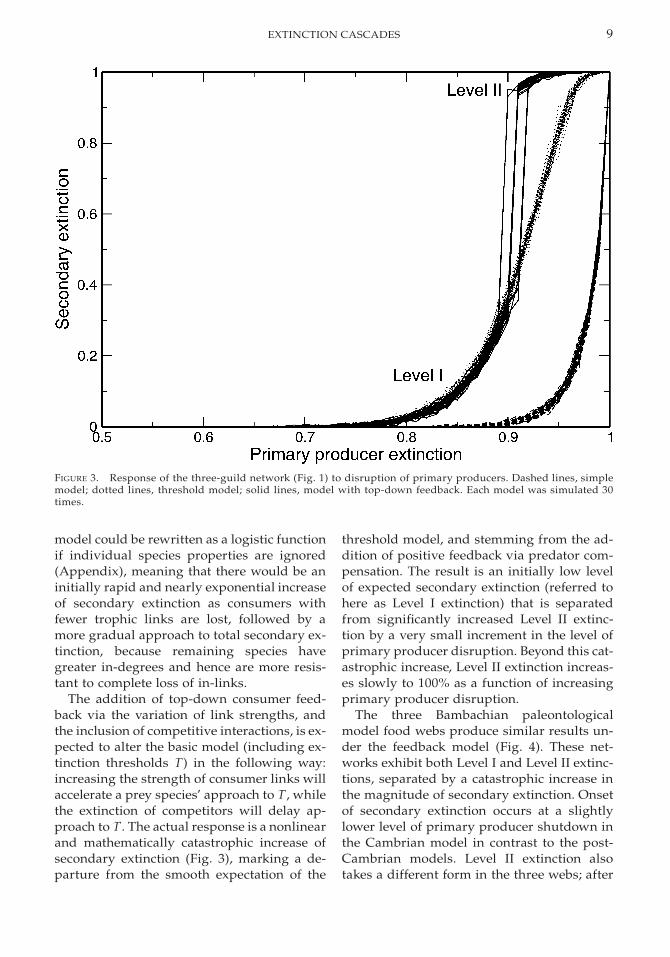
FIGURE 3. Response of the three-guild network (Fig. 1) to disruption of primary producers. Dashed lines, simplemodel; dotted lines, threshold model; solid lines, model with top-down feedback. Each model was simulated 30times.

model could be rewritten as a logistic functionif individual species properties are ignored(Appendix), meaning that there would be aninitially rapid and nearly exponential increaseof secondary extinction as consumers withfewer trophic links are lost, followed by amore gradual approach to total secondary ex-tinction, because remaining species havegreater in-degrees and hence are more resis-tant to complete loss of in-links.

The addition of top-down consumer feed-back via the variation of link strengths, andthe inclusion of competitive interactions, is ex-pected to alter the basic model (including ex-tinction thresholds T) in the following way:increasing the strength of consumer links willaccelerate a prey species’ approach to T, whilethe extinction of competitors will delay ap-proach to T. The actual response is a nonlinearand mathematically catastrophic increase ofsecondary extinction (Fig. 3), marking a de-parture from the smooth expectation of the

threshold model, and stemming from the ad-dition of positive feedback via predator com-pensation. The result is an initially low levelof expected secondary extinction (referred tohere as Level I extinction) that is separatedfrom significantly increased Level II extinc-tion by a very small increment in the level ofprimary producer disruption. Beyond this cat-astrophic increase, Level II extinction increas-es slowly to 100% as a function of increasingprimary producer disruption.

The three Bambachian paleontologicalmodel food webs produce similar results un-der the feedback model (Fig. 4). These net-works exhibit both Level I and Level II extinc-tions, separated by a catastrophic increase inthe magnitude of secondary extinction. Onsetof secondary extinction occurs at a slightlylower level of primary producer shutdown inthe Cambrian model in contrast to the post-Cambrian models. Level II extinction alsotakes a different form in the three webs; after


FIGURE 4. Responses of the hypothetical paleontological food webs to disruption of primary producers, using themodel with top-down feedback. Circles, Cambrian food web. Squares, Post-Cambrian Paleozoic. Triangles, Me-sozoic. Solid lines with symbols represent the mean of 30 simulations, while dashed lines show 25% and 75% quar-tile ranges.

the catastrophe, secondary extinction tends tobe lower in the post-Cambrian models relativeto the Cambrian model, at any given level ofprimary producer shutdown.

Detailed examination of the responses of in-dividual megaguilds to primary productiondisruption in each simulation explains thesummary differences noted above. Figure 5 il-lustrates the results for three individual me-gaguilds in the three models. The responses ofpelagic suspension feeders vary very littleamong the models (Fig. 5A–C), even thoughthe trophic relationships vary; pelagic carni-vores prey on pelagic suspension feeders inthe post-Cambrian models only. This meansthat the dynamics of this particular mega-guild are controlled primarily by its responseto bottom-up perturbation. The impact of pre-

dation in the post-Cambrian models is mini-mized by the broad diets assigned to pelagiccarnivores in those models. The responses ofcarnivore guilds, on the other hand, are func-tions of the relative taxonomic diversities ofpredators and prey, as well as the complexityof the trophic connections assigned to thepredators. For example, Cambrian infaunalcarnivores (Fig. 5D) exhibit low levels of LevelI secondary extinction, followed by a signifi-cant catastrophic increase that results bothfrom bottom-up generated prey extinctionsand top-down feedback from the carnivoresthemselves. Epifaunal carnivores, which arenot present in the Cambrian model, exhibitmore complicated response patterns in thepost-Cambrian models (Fig. 5E,F). This groupexhibits an initial catastrophe at the point at


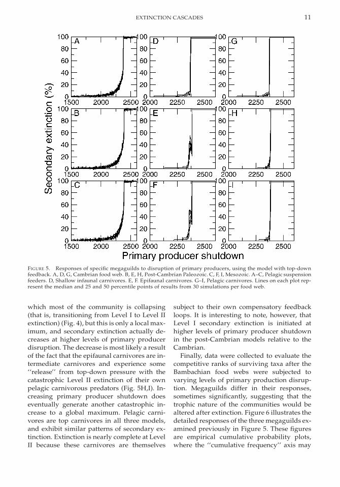
FIGURE 5. Responses of specific megaguilds to disruption of primary producers, using the model with top-downfeedback. A, D, G, Cambrian food web. B, E, H, Post-Cambrian Paleozoic. C, F, I, Mesozoic. A–C, Pelagic suspensionfeeders. D, Shallow infaunal carnivores. E, F. Epifaunal carnivores. G–I, Pelagic carnivores. Lines on each plot rep-resent the median and 25 and 50 percentile points of results from 30 simulations per food web.

which most of the community is collapsing(that is, transitioning from Level I to Level IIextinction) (Fig. 4), but this is only a local max-imum, and secondary extinction actually de-creases at higher levels of primary producerdisruption. The decrease is most likely a resultof the fact that the epifaunal carnivores are in-termediate carnivores and experience some‘‘release’’ from top-down pressure with thecatastrophic Level II extinction of their ownpelagic carnivorous predators (Fig. 5H,I). In-creasing primary producer shutdown doeseventually generate another catastrophic in-crease to a global maximum. Pelagic carni-vores are top carnivores in all three models,and exhibit similar patterns of secondary ex-tinction. Extinction is nearly complete at LevelII because these carnivores are themselves

subject to their own compensatory feedbackloops. It is interesting to note, however, thatLevel I secondary extinction is initiated athigher levels of primary producer shutdownin the post-Cambrian models relative to theCambrian.

Finally, data were collected to evaluate thecompetitive ranks of surviving taxa after theBambachian food webs were subjected tovarying levels of primary production disrup-tion. Megaguilds differ in their responses,sometimes significantly, suggesting that thetrophic nature of the communities would bealtered after extinction. Figure 6 illustrates thedetailed responses of the three megaguilds ex-amined previously in Figure 5. These figuresare empirical cumulative probability plots,where the ‘‘cumulative frequency’’ axis may


FIGURE 6. Distributions of competitive rank for specific megaguilds at varying levels of primary producer disrup-tion. Higher values (x-axis) indicate higher competitive rank. Arrangement of food webs and megaguilds followsthat in Figure 5. Levels of primary producer disruption are given in the text. Plots (lines) are mean cumulativefrequencies, at a given competitive rank, from 30 simulations.

be interpreted as the proportion of the under-lying distribution that is less than or equal toa particular competitive rank. Each distribu-tion in this case describes competitive ranks ina megaguild. The slope of a plot measures therate at which observations accumulate as com-petitive rank is increased, indicating the gen-eral shape of the underlying probability den-sity. For example, the straight diagonal lineson all the plots mean that observations are ac-cumulating uniformly, suggesting underlyinguniform distributions. This is indeed the casefor the starting distributions of competitiveranks in the simulations. Upward-curving(concave up) plots indicate the slow accumu-lation of taxa, and hence underlying distri-butions weighted toward competitively su-perior taxa, whereas concave down plots in-

dicate distributions with a predominance ofcompetitively inferior taxa. Three plots aregiven for each megaguild, showing the distri-butions of competitive rank at the followinglevels of primary producer disruption: 2080(80%), 2340 (90%), and 2418 (93%). Thesethree points capture low levels of secondaryextinction, increasing Level I, and Level II sec-ondary extinction respectively.

There is very little deviation from unifor-mity, or variation among the models, for pe-lagic suspension feeders (Fig. 6A–C). Cambri-an shallow infaunal carnivores likewise exhib-it little departure from uniformity (Fig. 6D),suggesting that members of these megaguildshave roughly equal probabilities of survivingecosystem collapse, regardless of competitiveabilities. The situation is different for epifau-


FIGURE 7. Distributions of competitive rank of two additional megaguilds. A–C, Epifaunal suspension feeders. D–F, Shallow infaunal deposit feeders. A, D, Cambrian food web. B, E, Post-Cambrian Paleozoic. C, F, Mesozoic. Sig-nificant convexity of cumulative frequency plots indicates predominance of competitively inferior taxa.

nal carnivores in the post-Cambrian models,however, with a greater survivorship of com-petitively superior taxa in the Paleozoic model(Fig. 6E), but greater survivorship of taxa oflow to intermediate abilities in the post-Paleo-zoic model (Fig. 6F). Pelagic carnivores arelikewise variable, with distinctly greater sur-vivorship of competitive superiors in theCambrian model (Fig. 6G), but slightly greater

survivorship of competitive inferiors in thepost-Cambrian models (Fig. 6H,I).

Relative survivorship of competitors wasexamined in detail for two additional mega-guilds, epifaunal suspension feeders and shal-low infaunal deposit feeders (Fig. 7), both be-cause of the good representation of these taxain the fossil record and because they serve todemonstrate the variability among the mod-


els. The dramatic plot in Figure 7A shows thatLevel II extinction generates a distributionpeaked at low competitive rank. The guild ofepifaunal suspension feeders should be dom-inated by competitively inferior taxa after aLevel II extinction within a Cambrian com-munity (Fig. 7A), but would have only a slightpredominance of taxa of intermediate com-petitive rank in post-Cambrian communities(Fig. 7B,C). Level II shallow infaunal depositfeeder survivors, however, are dominated bytaxa of relatively low competitive rank in allthe models (Fig. 7D–F).

Discussion

Predictions of bottom-up driven cascades ofsecondary extinction (Quince et al. 2005),combined with observations that primary pro-duction is often disrupted severely duringtimes of mass extinction, suggest that suchdisruption could account for significant pro-portions of the diversity lost during those in-tervals of extinction. Studies of perturbation ofmodern ecosystems further suggest that cas-cades probably do not follow simple linearrules of cause (loss of primary production)and effect (consequential loss of consumers)(Williams et al. 2002), but rather that the con-sequences of a loss of productivity are emer-gent from the complex networks of trophicand other biotic interactions. The model pre-sented in this paper combined bottom-up(production) and top-down (consumption) in-teractions (Worm and Duffy 2003), as well asintraguild competitive interactions, with verygeneral hypotheses of food web variationthrough the Phanerozoic, to examine how dis-ruption of primary production affects second-ary extinction and extinction cascades. In spiteof critical information that can be difficult toobtain for fossil communities, for example thespecific details of intimate biotic interactions,our growing understanding of the nature anddistributions of interactions in modern com-munities serves as a guide.

The model simulations were parameterizedusing reasonable inferences, based on currentpaleoecological knowledge, of taxonomic rich-ness and of guild and functional diversities.Specifying parameter values when those pa-rameters might range broadly raises concerns

of overparameterization and model specificity(May 2004). A partial solution is the broad ex-ploration of parameter sets and combinationsin order to evaluate, at least qualitatively, theimpact of parameter values on the model. Thatis essentially the approach adopted in this pa-per, as well as by Angielczyk et al. (2005) in anempirical application of the model to specificLate Permian terrestrial communities. An al-ternative approach, which also requires exten-sive empirical data, is the inference of modelparameters from the data themselves (see be-low). Nevertheless, the following interestingobservations emerge from the exploratory ap-plication of the model to the hypotheticalBambachian food webs.

Increasing the level of primary productiondisruption (v) increases the magnitude of sec-ondary extinction in all food webs. The maincause of secondary extinction is the loss of pri-mary consumers as they are increasingly de-prived of their sources of food. This loss ispropagated through the trophic network tosecondary and higher consumers, but reason-able assumptions of consumer behavior sug-gest that those consumers should compensatefor the loss of a trophic resource or prey taxonby increasing the intensities of their interac-tions with remaining prey taxa. The result istop-down exacerbation of the stress experi-enced by prey taxa, thereby accelerating theirapproach to extinction thresholds. This posi-tive top-down feedback elevates the level ofsecondary extinction caused by any particularlevel of disruption of primary production tothe point where a positive feedback-loopamong the trophic levels causes a catastrophicincrease of secondary extinction. Therefore,two distinct forms of secondary extinctionmay exist for any guild within the network:Level I, where secondary extinction is largelythe result of bottom-up propagation, and Lev-el II, where positive top-down feedback con-tributes to catastrophic increases in secondaryextinction.

The level of secondary extinction that re-sults from any given magnitude of v dependsultimately on the general complexity of thetrophic network, that is, the number of me-gaguilds and the geometry of the trophic con-nections among them. This is illustrated clear-


ly by comparing the hypothetical Cambrianand post-Cambrian networks. The absence ofdirect predation, or a limited number of pred-ators on a consumer guild, such as pelagic sus-pension feeders, means that secondary extinc-tion, both Level I and II, is largely a functionof the increasing loss of primary producer re-sources (v) (Fig. 5A–C). The addition of pre-dation, however, and the top-down compen-satory feedback of predators, can result in var-iable and complicated patterns of Level I andLevel II secondary extinction. Epifaunal car-nivores exhibit such patterns in the post-Cam-brian models (Fig. 5E,F). There are two max-ima of secondary extinction: after an initialand rapid increase, the secondary extinctionresponse declines drastically, only to increasecatastrophically at a yet higher level of pri-mary producer disruption.

Overall, the increasing number of connec-tions among megaguilds during the Phaner-ozoic, representing increases in functional di-versity, serve to delay the onset of secondaryextinction and catastrophic cascades of extinc-tion. For example, compare the carnivoresamong the three models. The onset of second-ary extinction occurs at increasingly higherlevels of primary producer shutdown throughthe Phanerozoic in both the epifaunal carni-vores (Fig. 5E,F) and pelagic carnivores (Fig.5G,H). This would suggest increasing com-munity resistance to such extinctions throughthe Phanerozoic (Tang 2001). Community sta-bility also increases, if one defines stability asa transition among different community‘‘states,’’ because the top-down driven tran-sition to Level II, though it occurs in all me-gaguilds in all the models, can sometimes bedampened (for example, in the post-Cambrianepifaunal carnivores).

One potential mechanism opposing the top-down feedback loop is the extinction of intra-guild competitors. For any consumer species,the loss of a competitor might ameliorate theimpact of the loss of trophic resources and in-creasing predation intensity. This mechanismwas examined in the model networks by rank-ing members of each megaguild uniformlyand allowing the extinction of competitive su-periors to restrain a species’ approach to ex-tinction thresholds. The inclusion of compet-

itive interactions in the model does not alterthe occurrence of catastrophic secondary ex-tinction, implying that those interaction termsare overwhelmed by the bottom-up pertur-bations and top-down feedback in the simu-lations. Interesting patterns of differential sur-vival do, however, emerge from the simula-tions. In several megaguilds, top-down com-pensatory feedback interacts with competitionto result in the increased probability of surviv-al of competitively inferior taxa. This result canbe understood qualitatively if one considersthat for a competitively superior species, theloss of a fellow guild member has little or nooffsetting effect on the acquisition of trophicresources, whereas for an inferior species, theloss of a competitive superior releases other-wise unavailable resources, allowing it to ex-pand its realized niche (Hutchinson 1957). Theonly groups that display this result, however,are those prey guilds involved in simple pred-ator-prey networks, that is, having a singlepredatory guild. For example, epifaunal sus-pension feeders are preyed upon solely by pe-lagic carnivores in the Cambrian model, andthe distribution of Level II survivors is onedominated by competitively inferior taxa. Thepattern is not present in the post-Cambrianmodels where epifaunal suspension feedersare involved in more complex trophic net-works, involving intermediate epifaunal car-nivores. Shallow infaunal deposit feeders, onthe other hand, remain in essentially isolatedsub-communities in all three models involv-ing predation solely by top shallow infaunalcarnivores. The preferential survival of com-petitively inferior taxa is persistent in this me-gaguild.

The predominance of such taxa in cohorts ofsurvivors in the simulations is very reminis-cent of empirically observed post-extinction‘‘disaster’’ taxa (Schubert and Bottjer 1992).Disaster taxa have been described as oppor-tunistic generalists because of their increasedrepresentation and ranges after mass extinc-tion events. These taxa would be recognizedon ecological timescales as early colonizersand perhaps ‘‘weedy’’ species. Their emer-gence from the simulations might be impor-tant validation of the model and is not withoutprecedent in studies of modern communities


(Nielsen and Navarrete 2004). Interestingly,skewed survivor distributions, with a pre-dominance of inferior competitors, has alsobeen observed in terrestrial plant communi-ties of the Permo-Triassic (Looy et al. 2001)and is consistent with models of extinction inmodern plant communities (Tillman et al.1994; Loehle and Li 1996). The model pre-sented here suggests that the dominance ofsuch taxa in post-Level II extinction commu-nities is largely a function of their pre-extinc-tion trophic ecologies and their trophic con-nectedness. The model therefore predicts thatsuch differential patterns of survival amongvarious megaguilds (for example, compareepifaunal suspension feeders and infaunal de-posit feeders in the post-Cambrian webs)should be observed only when bottom-updriven, Level II ecosystem collapse was themechanism of secondary extinction. Further-more, Level II secondary extinction is one pos-sible mechanism for generating the ecosys-tem-replacing Category I extinctions de-scribed by Droser et al. (2000) (see alsoMcGhee et al. 2004).

Parameter Determination. The parameterranges of the numerical model define a broadparameter space, and exploration of theseranges should yield additional insight intosecondary extinction in ancient communities.For example, the effect of nonrandom extinc-tions or perturbations of primary producerscould provide insight into similar perturba-tions of modern ecosystems, or the use of awider range of power law distributions for de-termining the in-degrees of species would re-sult in different ranges of trophic specializa-tion. As mentioned earlier, however, even ifparameter ranges could be limited by reliableecological insight, exploring the possible setsof parameter combinations would still requirea prohibitively large number of simulations. Itis tempting to use a forward model such asthis one to search for and tune parameter setsthat produce observed extinction data. Giventhe complexity of the model, however, and thecomplexity of the systems that it seeks to de-scribe, it is quite likely that different parame-ter sets are capable of producing similar re-sults. Exploration of parameter ranges as asearch tool for an extinction level is therefore

neither feasible nor desirable, unless very spe-cific empirical sample-level paleocommunitydata were available. In that case, one alterna-tive would be to use data comprising pre- andpostextinction measures of ecosystem com-position, along with the model, to estimate pa-rameter posterior probability densities. Bayes’formula would be used to explore the param-eter space of the model and data, estimatingthe posterior distribution of extinction param-eters for the feedback model. A Bayesian for-mulation of the feedback model may be writ-ten as

p(C z u)p(u)p(u z C) 5 (10)

p(C)

where c is a vector of the observed within-guild extinction data, u are the model param-eters (5N, , ) (Appendix), of which andg v g

and are unknown, and p(c) 5 # p(c z u)p(u)vdu is the normalizing constant. N is a vectorof guild taxonomic diversities, is a vector ofgdegree distribution (power law) coefficients,and is a vector (or scalar) denoting levels ofvprimary producer disruption. Both N and gare of a size equal to the number of guilds. Anexplicit solution of the formula is impossiblegiven the high dimensionality of u and thecomplexity of the problem, but evaluationshould be possible via stochastic simulation ofp(u z c), for example using Markov Chain Mon-te Carlo sampling or other types of Metropo-lis-Hastings sampling algorithms (Metropoliset al. 1953; Marjorum et al. 2003).

Recovery. The catastrophic shift betweenLevel I and II extinctions, in response to theperturbation of primary production, may bearimplications for the subsequent recovery ofecosystems that experience Level II extinction.It has been hypothesized that ecosystemswhich undergo a dramatic shift in state as aresult of environmental perturbation willshow hysteresis patterns of recovery (Schefferet al. 2004; van Nes and Scheffer 2004). In oth-er words, simple reversal of the perturbationpast the point of catastrophe will not reversethe state of the system, but reversal must in-stead extend to some point that triggers an-other dramatic shift, this time back to the pre-perturbation state. If this is the case for LevelI to II transition, then ecosystems would be ex-


pected to display extended periods of recov-ery from mass extinctions that involved eco-system collapse (Looy et al. 1999; Benton et al.2004; Pruss and Bottjer 2004). Level II extinc-tion would also then be a potential explana-tion of the ecosystem-destroying Category Iextinctions defined by McGhee et al. (2004).Recovery would depend upon the recovery ofprimary production, the evolution of addi-tional taxa from the survivors, and the assem-bly of new ecosystems. These issues could beexplored by coupling output from the currentmodel with models of ecosystem recovery(Sole et al. 2002) and evolution (Drossel et al.2001; Quince et al. 2005).

Acknowledgments

I am very grateful to E. Conel for her dedi-cation and hard work on this project. The pa-per benefited greatly from discussions with D.Goodwin, L. Leighton, D. Lindberg, and par-ticularly K. Angielczyk, C. Tang, G. Vermeij,and S. Wang. M. Foote and R. Plotnick provid-ed very helpful and insightful reviews.

Literature CitedAlbert, R., H. Jeong, and A. Barabasi. 2000. Error and attack tol-

erance in complex networks. Nature 406:378–382.Allmon, W. D. 2001. Nutrients, temperature, disturbance, and

evolution: a model for the late Cenozoic marine record of thewestern Atlantic. Palaeogeography, Palaeoclimatology, Pa-laeoecology 166:9–26.

Anderson, L. C. 2001. Temporal and geographic size trends inNeogene Corbulidae (Bivalvia) of tropical America: using en-vironmental sensitivity to decipher causes of morphologictrends. Palaeogeography, Palaeoclimatology, Palaeoecology166:101–120.

Angielczyk, K. D., P. D. Roopnarine, and S. C. Wang. 2005. Mod-eling the role of primary productivity disruption in end-Permian extinctions, Karoo Basin, South Africa. Bulletin ofthe New Mexico Museum of Natural History (in press).

Bambach, R. K. 1977. Species richness in marine benthic habitatsthrough the Phanerozoic. Paleobiology 3:152–167.

———. 1983. Ecospace utilization and guilds in marine com-munities through the Phanerozoic. Pp. 719–746 in M. Teveszand P. McCall, eds. Biotic interactions in Recent and fossilbenthic communities. Plenum, New York.

———. 1993. Seafood through time: changes in biomass, ener-getics, and productivity in the marine ecosystem. Paleobiol-ogy 19:372–397.

Benton, M. J., and R. J. Twitchett. 2003. How to kill (almost) alllife: the end-Permian extinction event. Trends in Ecology andEvolution 18:358–365.

Benton, M. J., V. P. Tvredokhlebov, and M. V. Surkov. 2004. Eco-system remodelling among vertebrates at the Permian-Trias-sic boundary in Russia. Nature 432:97–100.

Borrvall, C., B. Ebenman, and T. Jonsson. 2000. Biodiversity less-ens the risk of cascading extinction in model food webs. Ecol-ogy Letters 3:131–136.

Brown, J. H. 1995. Macroecology. University of Chicago Press,Chicago.

Camacho, J., R. Guimera, and L. A. N. Amaral. 2002. Robust pat-tern in food web structures. Physical Review Letters 88(22):228102-1–228102-4.

de Ruiter, P. C., V. Wolters, J. C. Moore, and K. O. Winemiller.2005. Food web ecology: playing jenga and beyond. Science309:68–71.

Droser, M. L., D. J. Bottjer, P. M. Sheehan, and G. R. McGhee.2000. Decoupling of taxonomic and ecologic severity of Phan-erozoic marine mass extinctions. Geology 28:675–678.

Drossel, B., P. G. Higgs, and J. A. McKane. 2001. The influenceof predator-prey population dynamics on the long-term evo-lution of food web structure. Journal of Theoretical Biology208:91–107.

Dunne, J. A., R. J. Williams, and N. D. Martinez. 2002. Food-webstructure and network theory: the role of connectance andsize. Proceedings of the National Academy of Sciences USA99:12917–12922.

Elton, C. 1927. Animal ecology. University of Chicago Press,Chicago.

Eshet, Y., M. R. Rampino, and H. Visscher. 1995. Fungal eventand palynological record of ecological crisis and recoveryacross the Permian-Triassic boundary. Geology 23:967–970.

Falkowski, P. G., M. E. Katz, A. H. Knoll, A. Quigg, J. A. Raven,O. Schofield, and F. J. R. Taylor. 2004. The evolution of moderneukaryotic plankton. Science 305:354–360.

Foster, C. B., M. H. Stephenson, C. Marshall, G. A. Logan, andP. F. Greenwood. 2002. A revision of Reduviasporonites Wilson1962: description, illustration, comparison and biological af-finities. Palynology 26:35–58.

Goldwasser, L., and J. Roughgarden. 1993. Construction andanalysis of a large Caribbean food web. Ecology 74:1216–1233.

———. 1997. Sampling effects and the estimation of food-webproperties. Ecology 78:41–54.

Hairston, N. G., F. E. Smith, and L. B. Slobodkin. 1960. Com-munity structure, population control, and competition. Amer-ican Naturalist 94:421–425.

Havens, K. 1992. Scale and structure in natural food webs. Sci-ence 257:1107–1109.

Hutchinson, G. E. 1957. Concluding remarks. Cold Spring Har-bour Symposium on Quantitative Biology 22:415–427.

Knoll, A. H., and R. K. Bambach. 2000. Directionality in the his-tory of life: diffusion from the left wall or repeated scaling ofthe right. In D. H. Erwin and S. L. Wing, eds. Deep time: Pa-leobiology’s perspective. Paleobiology 26(Suppl. to No. 4):1–14.

Knoll, A. H., R. K. Bambach, D. E. Canfield, and J. P. Grotzinger.1996. Comparative Earth history and Late Permian mass ex-tinction. Geology 273:452–457.

Lande, R., and S. Engen, and B. Sæther. 2003. Stochastic popu-lation dynamics in ecology and conservation. Oxford Univer-sity Press, Oxford.

Leighton, L. R. 2004. Are we asking the right question? Palaios19:313–315.

Levinton, J. S. 1996. Trophic group and the end-Cretaceous ex-tinction: did deposit feeders have it made in the shade? Pa-leobiology 22:104–112.

Lindeman, R. 1942. The trophic-dynamic aspect of ecology.Ecology 23:399–418.

Loehle, C., and B. Li. 1996. Habitat destruction and the extinc-tion debt revisited. Ecological Applications 6:784–789.

Looy, C. V., W. A. Brugman, D. L. Dilcher, and H. Visscher. 1999.The delayed resurgence of equatorial forests after the Perm-ian-Triassic ecologic crisis. Proceedings of the National Acad-emy of Sciences USA 96:13857–13862.

Looy, C. V., R. J. Twitchett, D. L. Dilcher, and J. H. A. V. K.-V.


Cittert. 2001. Life in the end-Permian dead zone. Proceedingsof the National Academy of Sciences USA 98:7879–7883.

Marjorum, P., J. Molitor, V. Plagnol, and S. Tavare. 2003. Markovchain Monte Carlo without likelihoods. Proceedings of theNational Academy of Sciences USA 100:15324–15328.

Martin, R. E. 1996. Secular increase in nutrient levels throughthe Phanerozoic: implications for productivity, biomass, di-versity, and extinction of the marine biosphere. Paleontolog-ical Journal 30:637–643.

Martinez, N. D. 1992. Constant connectance in community foodwebs. American Naturalist 139:1208–1218.

May, R. M. 1973. Stability and complexity in model ecosystems.Princeton University Press, Princeton, N.J.

———. 2004. Uses and abuses of mathematics in biology. Science303:790–793.

McCann, K., A. Hastings, and G. R. Huxel. 1998. Weak trophicinteractions and the balance of nature. Nature 395:794–798.

McGhee, G. R., P. M. Sheehan, D. J. Bottjer, and M. L. Droser.2004. Ecological ranking of Phanerozoic biodiversity crises:ecological and taxonomic severities are decoupled. Palaeo-geography, Palaeoclimatology, Palaeoecology 211:289–297.

Metropolis, N., A. W. Rosenbluth, M. N. Rosenbluth, and A. H.Teller. 1953. Equation of state calculations of fast computingmachines. Journal of Chemical Physics 21:1087–1092.

Montoya, J. M., and R. V. Sole. 2002. Small world patterns infood webs. Journal of Theoretical Biology 214:405–412.

Nielsen, K. J., and S. A. Navarrete. 2004. Mesoscale regulationcomes from the bottom up: intertidal interactions betweenconsumers and upwelling. Ecology Letters 7:31–41.

Olszewski, T. D., and D. H. Erwin. 2004. Dynamic response ofPermian brachiopod communities to long-term environmen-tal change. Nature 428:738–741.

Paine, R. T. 1992. Food-web analysis through field measurementof per capita interaction strength. Nature 355:73–75.

Peters, R. H. 1983. The ecological implications of body size.Cambridge University Press, Cambridge.

Pruss, S. B., and D. J. Bottjer. 2004. Early Triassic trace fossils ofthe Western United States and their implications for pro-longed environmental stress from the end-Permian mass ex-tinction. Palaios 19:551–564.

Quince, C., P. G. Higgs, and A. J. McKane. 2005. Deleting speciesfrom model food webs. Oikos 110:283–296.

Roopnarine, P. D. 1996. Systematics, biogeography and extinc-tion of chionine bivalves (Early Oligocene–Recent) in the LateNeogene of tropical America. Malacologia 38:103–142.

Scheffer, M., S. Carpenter, J. A. Foley, C. Folke, and B. Walker.2004. Catastrophic shifts in ecosystems. Nature 413:591–596.

Schubert, J. K., and D. J. Bottjer. 1992. Early Triassic stromato-lites as post-mass extinction disaster forms. Geology 20:883–886.

Sepkoski, J. J., Jr. 1981. A factor analytic description of the Phan-erozoic marine fossil record. Paleobiology 7:36–53.

———. 1984. A kinetic model of Phanerozoic taxonomic diver-sity. Paleobiology 10:246–267.

Sheehan, P. M., and T. A. Hansen. 1986. Detritus feeding as abuffer to extinction at the end of the Cretaceous. Geology 14:868–870.

Sole, R. V., J. M. Montoya, and D. H. Erwin. 2002. Recovery aftermass extinction: evolutionary assembly in large-scale bio-sphere dynamics. Philosophical Transactions of the Royal So-ciety of London B 357:697–707.

Tang, C. M. 2001. Stability in ecological and paleoecological sys-tems: variability at both short and long timescales. Pp. 63–81in W. D. Allmon and D. J. Bottjer, eds. Evolutionary paleo-ecology. Columbia University Press, New York.

Tillman, D., R. M. May, C. L. Lehman, and M. A. Nowak. 1994.Habitat destruction and the extinction debt. Nature 371:65–66.

Todd, J. A., J. B. C. Jackson, K. G. Johnson, H. M. Fortunato, A.Heitz, M. Alvarez, and P. Jung. 2002. The ecology of extinc-tion: molluscan feeding and faunal turnover in the CaribbeanNeogene. Proceedings of the Royal Society of London B 269:571–577.

Vajda, V., and S. McLoughlin. 2004. Fungal proliferation at theCretaceous-Tertiary boundary. Science 303:1489.

van Nes, E. H., and M. Scheffer. 2004. Large species shifts trig-gered by small forces. American Naturalist 164:255–266.

Vermeij, G. J. 1987. Evolution and escalation: an ecological his-tory of life. Princeton University Press, Princeton, N.J.

———. 1995. Economics, volcanoes, and Phanerozoic revolu-tions. Paleobiology 21:125–152.

———. 2004. Ecological avalanches and the two kinds of extinc-tion. Evolution Ecology Research 6:315–337.

Vermeij, G. J., and E. J. Petuch. 1986. Differential extinction intropical American molluscs: endemism, architecture, and thePanama land bridge. Malacologia 17:29–41.

Visscher, H., H. Brinkhuis, D. L. Dilcher, W. C. Elsik, Y. Eshet,C. V. Looy, M. R. Rampino, and A. Traverse. 1996. The ter-minal Paleozoic fungal event: evidence of terrestrial ecosys-tem destabilization and collapse. Proceedings of the NationalAcademy of Sciences USA 93:2155–2158.

Wilf, P., and K. R. Johnson. 2004. Land plant extinction at theend of the Cretaceous: a quantitative analysis of the North Da-kota megafloral record. Paleobiology 30:347–368.

Williams, R. J., and N. D. Martinez. 2000. Simple rules yieldcomplex food webs. Nature 404:180–183.

Williams, R. J., E. L. Berlow, J. A. Dunne, A. Barabasi, and N. D.Martinez. 2002. Two degrees of separation in complex foodwebs. Proceedings of the National Academy of Sciences USA99:12913–12916.

Worm, B., and J. E. Duffy. 2003. Biodiversity, productivity andstability in real food webs. Trends in Ecology and Evolution18:628–632.

Zachos, J. C., M. A. Arthur, and W. F. Dean. 1989. Geochemicalevidence for suppression of pelagic marine productivity atthe Cretaceous/Tertiary boundary. Nature 337:61–64.

Appendix

1. There is a set of links, R, mapping consumers to prey re-sources in the set M. The number of links (size of R) is de-noted as #(R) 5 r1, with 0 , r1 # #(M). Let #(M) 5 M. v re-sources are eliminated randomly from M, with 0 , v # M.If W is the set of eliminated resources, then W , M and #(W)5 v. The probability that R → W, that is, the set of consumerlinks all correspond to eliminated resources is

21M 2 r M1p(e z v) 5r1 1 21 2v 2 r v1

(M 2 r )! v!(M 2 v)!15

(v 2 r )!(M 2 r 2 v 1 r )! M!1 1 1

v!(M 2 r )!15 .

M!(v 2 r )!1

2. The expected, or mean, number of secondary extinctions (c)given the above probability is

v

c 5 p(e z v)p (r )NO r 1 11r 511

where p(r1)N1 is the expected number of consumer taxa withr1 in-links. c is the summation of expected extinctions givenconsumer taxa with 0 , r1 # v, and is reduced algebraicallyas follows:


21v M 2 r M1c 5 p (r )NO 1 11 21 2v 2 r vr 51 11

v vv!(M 2 r )! N v! (M 2 r )!1 1 1⇒ N p (r ) ⇒ p (r ).O O1 1 1M!(v 2 r )! M! (v 2 r )!r 51 r 511 11 1

3. The hypergeometric formula describes the number of differ-ent ways that, given M potential prey, r consumer links, anda prey extinction level of v, exactly n of the consumer’s linkswill be lost. Because the mean of the resulting hypergeome-tric distribution in this case is rv/M, then equation (6) maybe derived as follows. Define an extinction threshold T rang-ing between 0 and 1, and set extinction to occur when theratio of the carrying capacity of the population with n linksto carrying capacity with r links falls below T . Because bothT and the ratio have a maximum value of 1, and carrying ca-pacity is equivalent to the number of incoming links, this def-inition can be expressed as

np (e z v) 5 1 2 .

r

4. The feedback loops cannot be formulated explicitly, but theycan be summarized symbolically as follows. Up until thispoint, the model has operated at geological timescales, abovethe ecological and generational scales of organisms. The ba-sic model (eq. 2) can be expressed as

E(c z v) 5 N1· f [M, v, P(r )].1,t N1

That is, expected extinction in guild N1 is the product of di-versity in that guild and a function of available primary pro-duction (M), primary producer shutdown (v) and the prob-ability distribution of N1’s trophic links. Feedback from theconsumers of guild N1, those are species in guild N2, is in-corporated as

E(c z v) 5 N1 · f [M, v, P(r ), P(S ), P(C )]1,t N1 N2,t N1

where P(SN2,t) is the distribution of link strengths in N2, andP(CN1) is the distribution of competitive ranks in N1, at timet. t is an approximately single-valued subdivision of thelarger (geologic) time interval t, e.g. organismal generations,with t K t. Given consumer compensation for lost links,

P(S ) 5 f [P(r ), N1 ]N2,t21 N2 t21

and expressing guild diversity at a point in time as a functionof earlier diversity, where

N1 ø N1 2 E(c z v),t21 t22 1,t22

then network-mediated extinction with positive feedbackmay be expressed as

E(c z v) 5 N1 · f [M, v, P(r ), P(r ), N1 , (c z v)].1,t12 t12 N1 N2 t 1,t

5. The basic model can be expressed as an ordinary differentialequation if we assume a simple linkage relationship betweenconsumers and prey. Let N be the number of consumer spe-cies, v the number of prey extinctions, and c the resultingnumber of secondary consumer extinctions. Then c 5 N(v)when v . 0 means that secondary extinction is a function ofthe number of consumers and the level of prey extinction.This leads to the rate relationship

dc5 lc

dv

which yields the general solution

lvc 5 c e0

where l is a constant, and c0 is the initial level of secondaryextinction. Setting the latter value to one, then when v 5 M(complete extinction of prey), and therefore c 5 N (completesecondary extinction), we derive

lMN 5 e ⇒ ln(N ) 5 lM ⇒ l 5 ln(N )/M.

Therefore, a general solution of the basic model is

vc 2 exp ln(N )[ ]M

which is qualitatively similar to the probabilistic basic model.The differential equation model cannot be extended easily,however, to accommodate individual guild and species prop-erties such as varying link distributions, extinction thresh-olds, and compensatory feedback.

6. List of notationP—probability of eventp(e z x)—probability of taxon extinction given the occurrence

of xv—level of primary producer shutdown or extinctionr—taxon’s in-degree, or number of incoming trophic linksci—level of secondary extinction in guild iE—expected, or mean levelP(x)—probability density of xT—taxon’s extinction threshold based on population size, or

number of available trophic resources (prey taxa)Ki—taxon’s carrying capacity given i trophic resourcesS—predation intensity on a taxon, measured as the sum of

predators’ link strengthsR—competitive rank of a taxon within its megaguildg—exponential coefficient of power law distributionp(u z C)—posterior probability of extinction model u given

observed extinction data Cp(C z u)—likelihood of observed extinction data C given ex-

tinction model up(u)—prior probability of extinction model u

extinction cascades and catastrophe in ancient food webs

Documents