export performance and its determinants: supply … models_marco/export perfomance.pdf ·...

UNITED NATIONS CONFERENCE ON TRADE AND DEVELOPMENT

POLICY ISSUES IN INTERNATIONAL TRADE AND COMMODITIES

STUDY SERIES No. 26

EXPORT PERFORMANCE AND ITS DETERMINANTS: SUPPLY AND DEMAND CONSTRAINTS

by

Marco Fugazza

Associate Economic Affairs Officer Trade Analysis Branch

Division on International Trade in Goods and Services, and Commodities United Nations Conference on Trade and Development

Geneva, Switzerland

UNITED NATIONS

New York and Geneva, 2004

ii

NOTE

The views expressed in this study are those of the author and do not necessarily reflect the views of the United Nations.

The designations employed and the presentation of the material do not imply the expression of any opinion whatsoever on the part of the United Nations Secretariat concerning the legal status of any country, territory, city or area, or of its authorities, or concerning the delimitation of its frontiers or boundaries.

Material in this publication may be freely quoted or reprinted, but acknowledgement is requested, together with a reference to the document number. It would be appreciated if a copy of the publication containing the quotation or reprint were sent to the UNCTAD secretariat:

Chief Trade Analysis Branch

Division on International Trade in Goods and Services, and Commodities United Nations Conference on Trade and Development

Palais des Nations CH-1211 Geneva

UNCTAD/ITCD/TAB/27

UNITED NATIONS PUBLICATION

Sales No. E.04.II.D.20

ISBN 92-1-112627-4

ISSN 1607-8291

© Copyright United Nations 2004 All rights reserved

iii

ABSTRACT

What are the major determinants of export performance? Does the importance of these

determinants vary with export performance itself? Using quantile regression techniques this study investigates the contribution towards the performance of the external sector of linkages to international markets relative to internal supply-side conditions. Results indicate that, while trade barriers continue to be of concern, poor supply-side conditions have often been the more important constraint on export performance in various regions, in particular in Africa and the Middle East, despite a generalized deepening of international trade integration. Beside strong linkages to international markets, good transport infrastructures, macroeconomic soundness and good quality institutions appear to be major determinants in the development process of the external sector.

iv

ACKNOWLEDGEMENTS

I am grateful to Sam Laird, who has improved significantly this study with extremely valuable comments and suggestions. I have benefited from discussions with Lucian Cernat, Jörg Mayer and Frédéric Robert-Nicoud. I also thank my colleagues at UNCTAD and seminar participants at the University of Geneva for their helpful comments.

v

CONTENTS

NON-TECHNICAL SUMMARY .......................................................................................1 INTRODUCTION .............................................................................................................3 I. THE THEORETICAL CONTEXT.........................................................................7 II. THE COMPONENTS OF GROWTH...................................................................9

(a) The Dataset ....................................................................................................... 9 (b) Estimation Strategy............................................................................................ 9 (i) Foreign market Access.......................................................................... 12

(ii) Supply Capacity ................................................................................... 19 (iii) Export Constraints ............................................................................... 20

(c) Sensitivity Analysis .......................................................................................... 24 III. EXPORT PERFORMANCE AND ITS DETERMINANTS.................................25

(a) An Extended Theoretical Framework............................................................... 25 (b) The Data ......................................................................................................... 25 (c) Estimation ....................................................................................................... 26 (d) Results and Interpretation................................................................................ 27

(i) General Considerations ........................................................................ 32 (ii) GDP and Population ........................................................................... 32 (iii) Internal Transport Frictions ................................................................. 32 (iv) The Macroeconomic Environment....................................................... 33 (v) Foreign Direct Investment ................................................................... 33 (vi) Institutions........................................................................................... 34 (vii) Foreign Market Access ......................................................................... 39

(e) Sensitivity Analysis........................................................................................... 40 IV. POLICY IMPLICATIONS....................................................................................41 V. POSSIBLE FURTHER RESEARCH .....................................................................43 REFERENCES...................................................................................................................44 APPENDIX ......................................................................................................................46

vi

Tables

1. Bilateral trade equation estimation ............................................................................ 10 2. Bilateral trade equation estimation with intra-regional trade dummies....................... 11 3. Components of export growth and regional concentration of foreign market access ............................................................................................. 14 4. Components of regional exports growth .................................................................... 17 5. Geographical composition of regional foreign market access growth.......................... 17 6. OLS regressions......................................................................................................... 28 7. Quantile regressions with institutions and paved roads .............................................. 29 8. Quantile regressions with Lab institutions and paved roads ....................................... 30 9. Quantile regressions with institutions, Lab institutions and paved roads.................... 31 10. Countries exports real value position in sample distribution ...................................... 35 11. Countries position in sample exports real value distribution ...................................... 37

Figures 1. Foreign market access and supply capacity................................................................. 13 2. Regional origin of foreign market access .................................................................... 18 Graph 1: Benchmarked export performance and components .............................................. 21

1

A strong and performing external sector is found in most country experiences to be thecompanion of a growing economy. The most striking and well-known example is the East Asiancountries experience. Identifying the elements that significantly affect export performance shouldfacilitate the design of policies to improve performance and ultimately overall economic growth.Such policies may also help to contain the negative effects on the trade balance that often occurimmediately following trade liberalization.

Determinants of export performance can be split into internal and external components.External factors are related to market access conditions and other factors affecting import demand.Apart from trade barriers and competition factors foreign market access is also determined bytransportation costs, which include geography and physical infrastructures. Internal factors referto supply-side conditions. Supply capacity is also affected by location-related elements, whichmay for example, affect access to raw materials and other resources. It also depends upon factorcosts such aslabour and capital. Beside resource endowment, factor costs are essentially the outcomeof economic policy and the institutional environment. Access to technology, which is likely toaffect the productivity of the external sector, may also be an important determinant.

In order to examine these issues, an econometric model of bilateral trade flows using gravitytechniques, was constructed. This model was tested using data series representing foreign marketaccess and supply capacity for a sample of 84 countries. It is thus possible to decompose exportperformance and identify the extent to which it has been constrained by its components.

The main findings are as follows: first, in the aggregate, all regions have benefited from thegreater integration of the world economy in the 1985-99 period. Access to extra-regional marketsin particular has been a key factor explaining export performance. However, intra-regionally-generated foreign market access has also been important in most regions, possibly underscoringthe increasing significance of regional trade agreements. However,this is not the case for the Sub-Sahara African countries whose intra-regional trade declined in all periods but 1992-95. In addition,African and Middle Eastern countries appear to have faced severe supply capacity constraints overthe last two decades, while their access to foreign markets has remained largely unchanged. EastAsian and Pacific countries’ export performance has been driven by equal improvements by bothsupply capacity and foreign market access. The export growth of South Asian countries can mainlybe explained by an important increase in their supply capacities.

The impact on export performance of various supply capacity factors controlling for foreignmarket access is investigated. This analysis used econometric techniques, namely quantile regressiontechniques that allow the consideration of possible non-linearities in the relationship betweenexport performance, supply capacity factors and foreign market access. It is thus possible to observerelationships between export performance and its components that vary with the level of exportperformance. It isalso possible to place the analysis in a development process framework, althoughlimited, by considering three successive periods.

NON-TECHNICAL SUMMARY

2

It was found that limitations on foreign market access are major contributors to poorexport performance. However, good performers in the second half of the 1990s also faced higherexternal constraints but were able to overcome them.

There is also evidence that exports can be expected to respond less than proportionally toa variation in import demand from abroad, although this not always true. In general theoretically,a rise in exports would tend to increase factors of production prices, which contain exportsexpansion.

Internal transport infrastructure captured by the percentage of paved roads is an importantsupply capacity element and is found to have a significant and positive impact in raising performance,as does a good macroeconomic environment. The contribution of foreign direct investment tocapital formation is included in order to include a technology-related element, possibly linked tothe structure of the external sector. The finding is that FDI is significant and has a positive impacton export performance at all levels.

The empirical results also suggest that foreign market access and the structure of the externalsector interact. So as the external sector expands and diversifies, domestic producers make aneffort to overcome supply capacity constraints and increase their capacity to meet new marketopportunities. The evolving structure of the external sector also makes a difference at all stages ofdevelopment and could dominate the role of international linkages at an intermediate stage ofstructural change. However, once a sector has reached structural “maturity”, as it seemed to be thecase for the best export performers among developed countries in the late 1990s, the significanceof foreign market access logically increases. In the present study, the institutional framework is ofmuch less importance than has been suggested in other recent studies in the empirical growthliterature.

The general policy implication is that foreign market access and supply capacity have to beconsidered equally important along the development process of the external sector. Simultaneousefforts to improve both supply capacity and foreign market access enhances the performance ofand the structural deepening of the external sector. Important elements of supply capacity at theearly stage of development of the external sector are transport infrastructure and macroeconomicstability. FDI is a significant determinant at all levels of export performance.

3

Despite the worldwide fall in trade barriers that has occurred in the last two decades,export performance has varied substantially across countries. World exports increased by almost220 per cent in twenty years. The figure jumps to 720 per cent for East Asian and Pacific countriesand falls to 80 per cent for Sub-Saharan countries. The exports of “best performers”, such as theRepublic of Korea, China, Cambodia and Viet Nam, have grown by more than 15 per cent annuallyover the whole period. “Worst performers”, mostly African and Latin American countries, havenegative annual growth rate records in at least one decade.

As a result of various trade negotiations and autonomous reforms, access to internationalmarkets has improved in the last twenty years. Nonetheless, it is likely that there is still much togain from further improvements in market access conditions. Concerns have also been raisedabout the necessity to improve supply conditions. Supply conditions are fundamental in definingthe export potential of an economy. For a given level of access to international markets, countrieswith better supply conditions are expected to export more.

This study investigates factors possibly explaining divergence in export performance.Particular attention is devoted to factors affecting supply conditions after controllingfor access tointernational markets.

The relevance of such an exercise rests also on the fact that no clear policy implicationsemerge from economic literature1 which looks at the relationship between open trade and economicgrowth. The positive correlation between output growth and export performance is a stronglyasserted empirical observation. Thus, a better knowledge of the determinants of export performanceshould contribute towards a better qualification of the relationship between open trade and growth.

Determinants of export performance can be split into external and internal components.External components include market access/entry conditions and a country’s location vis à visinternational markets. Internal components are related to supply-side conditions.

Foreign demand is influenced by various elements. Firstly , it is strongly linked to geography(the structural component). Typically, countries at the centre of a fast growing region are morelikely to benefit, ceteris paribus, than countries situated outside that region. Second, it is likely tobe related to competition and trade policy (the market access/entry component), which couldhave, in principle, a similar impact on trade than geography. Finally, both the quantity and qualityof physical infrastructures (the development component) are expected to play important roles.

INTRODUCTION

1 See Harrison (1996) for a review, Yanikkaya (2003) for a comprehensive review and set of estimates and Rodriguezand Rodrik (2000) for a re-examination of the relationship between trade policy and economic growth and acritical review of the literature.

4

Various elements are expected to affect supply-side conditions significantly. First of all,supply conditions are likely to be strongly related to location and the policy variables. The size ofthe country, which also determines the size of the internal market, together with the internalgeography of the country are the structural variables that could have an effect on the supplycapacity of a country. Economic policy could also be expected to affect supply capacity by affectingfactor prices. Development variables also have to be taken into consideration. They generallycorrespond to stock variables that are most often the outcome of previously implemented policies,such as public investment in transport infrastructures. Any measure related to general institutionaldevelopment could be relevant. Technology could also be seen as part of the development variablesset. In fact any variable able to capture prevailing technological conditions must be considered.

Recently Redding and Venables (2004a) investigated the relative contribution towards exportperformance of international linkages relative to internal geographical factors. They find thatmost of the differential in export performance of various countries and regions over the last threedecades can be due to differences in the evolution of external components. Nevertheless, they findthat internal components related to supply capacity such as internal geography and institutionalquality also have played a significant role in explaining the observed differential in exportperformance.

This study builds on the work of Redding and Venables. It uses the same theoretical modelof bilateral trade flows and adopt a similar empirical strategy. The latter initially consists of buildingdata series to capture the external components of export performance and, the whole the foreignmarket access component, using gravity techniques. Then, these series are used to investigate theimportance of foreign market access relative to supply capacity components. In other words, theexercise is to identify the possibl main determinants of the supply-side conditions after havingcontrolled for the external elements. However, this study has a different econometric approachfrom that used by Venables and Redding. Econometric techniques are used to control forunobservable country heterogeneity possibly affecting the real values of countries’ exports.Accounting for unobservable heterogeneity should allow the identification of any differences inthe effect of and importance of export performance components, which are linked to the degree ofdevelopment of the external sector itself. In other words, the techniques used here allow for thetesting for non-linearities in the relationship between export performance and its components.While dynamic panel techniques would seem to be the most desirable approach, data availabilityis likely to restrict their implementation. In this context, cross-sectional analysis proves to be aviable alternative. Regression techniques which are able to account for unobserved heterogeneityacross countries, namely quantile regressions, are used. Moreover, more emphasis is put on thedetermination and impact assessment of variables related to supply conditions. This is done withthe aim of determining as clearly as possible what are policy implications.2

The study reveals important differences across countries and regions when looking at theirrespective determinants of export performance. External and internal components prove to haveplayed an equal role in determining export performance for Asian countries. Their improvementin the South East and Pacific region appears to be high relative to that observed in any otherregion. Sub - Saharan African countries owe their export performance to the evolution of externalcomponents. The latter were strong enough to more than offset a relative deterioration of theirinternal production conditions.

2 In his comments on Redding and Venables (2004a), Maskus (2003) insists on the necessity to better identifysupply conditions variables in order to retrieve specific policy implications.

5

Further investigation also indicates that good internal conditions are necessary to obtaingood export performance. Particular attention should be paid to the macroeconomic dimension.Good infrastructures and non-stringent institutions are also necessary to put the export sector ona durable development path. In addition, there is scope for promoting a dynamic process ofdiversification across and within sectors. Constant efforts to support diversification are particularlyrelevant for commodities exporters when a secular downward trend is observed in volatilecommodities prices.

The next chapter presents the theoretical context. The empirical strategy adopted in orderto estimate exports components is presented in chapter II. Chapter III contains the empiricalapproach used to assess export performance. Chapter IV presents policy implications andconclusions.

7

Recently developed models of trade provide possible support for investigating the role ofsupply capacity in determining the export performance of a country. In particular, the Krugmanand Venables (1995) model identifies an empirically assessable decomposition of bilateral tradeinto market access and supply capacity. The theoretical framework is essentially a standard newtrade theory model based on product differentiation derived from a constant elasticity of substitutiondemand structure.

The economy consists of a number N of countries. Only the manufacturing sector isconsidered. Firms in that sector operate under increasing returns to scale and produce symmetricdifferentiated goods, which are used in consumption. Preferences are represented by a CES utilityfunction in which the elasticity of substitution σ between any pair of products is the same. Therepresentative utility function of country j is given by

( )( )1/

/1−

−

= ∑

σσσσ

N

iijij xnU σ > 1 (1)

where ni is the set of varieties produced in country i , and xij is the consumption in country j of asingle product variety from this set.

In that framework, the demand in country j for each variety produced in country i, is afunction of country’s j total expenditure on differentiated products Ej, the price of the good pij andthe price index Pj defined over the prices of individual varieties produced in i and sold in j. Totalexpenditure is assumed to be exogenously given. Demand for each variety writes as

( )1−−= σσjjijij PEpx

(2)

Where

[ ] ( )σσ −−∑=1/1

1ijij pnP

(3)

The elasticity of demand is identical across varieties and equal to σ. ( )1−σjj PE is a scale

factor that indicates the position of the demand curve in market j. The producer price pi is assumedto be the same for all varieties produced in country i. Transport frictions, which reflect the cost ofgetting a good from country i to country j, are set proportional to producers price. This cost iscomposed by three elements: the cost of getting the product to and from the border in countriesi and j (ti and tj respectively) and the cost of getting the product across the border (Tij). Intra-country cost would reflect internal geography and infrastructure. Inter-country cost would reflectexternal geography and policy barriers. Thus price

jijiiij tTtpp = and the value of total exports ofcountry i to country j is given by

( ) ( )111 −−−= σσσjjjijiiiijii PEtTtpnxpn (4)

I. THE THEORETICAL CONTEXT

8

Equation (4) is taken as the theoretical support for estimation of a gravity trade model. Itcan be rewritten as

( )[ ]( ) ( )( )[ ]111 / −−−= σσσiijijiiiijii tPETtpnxpn (4’)

The first term reflects the supply capacity of the exporting country, thereafter denoted b ysci. It is the product of the number of varieties and their price competitiveness, which is measuredby the product of the producer price and internal transport costs. The last term measures thetrans-border transport costs component. The first term into brackets is the market capacity ofcountry j, thereafter denoted by mj. It depends positively on total expenditures in j, on country jinternal transport costs and, on the number of competing varieties and their prices expressed inthe price index.

At the country level, that is looking at the total value of exports of country i, the followingis obtained

( )∑∑≠

−≠ ==

ijjijiij ijiii mTscxpnX σ1 (5)

The term ( )∑≠

−

ijjij mT σ1

represents country i foreign market access FMAi or equivalentlycountry i market potential which refers to the concept developed by Harris (1954). It correspondsto the sum of the market capacity of all country i exports destination countries, weighted bybilateral trade costs. Then, the product of supply capacity and foreign market access gives the totalvalue of exports of country.

The relative importance and evolution of these components are investigated empiricallyin the next chapter.

9

The model presented above postulates that the effect of a rise in expenditure on tradedgoods in a given country would benefit relatively more than those of its trading partners that arerelatively closer (the demand pecuniary effect). In this context, distance has to be interpreted notonly as a pure geographical element but also as any element that possibly represents a barrier totrade, such as tariffs, non-tariff barriers, anti-competitive barriers, etc.

The model also suggests that in order to capture fully the demand pecuniary effect justdescribed, favourable supply conditions are expected to play an essential role. In addition, equation(5) shows that access to foreign markets may be reduced by poor supply capacity.

(a) The Dataset

Bilateral trade flows for 84 countries are obtained from the UN COMTRADE database.Data are deflated by the United States GDP deflator in order to obtain real values. The base yearfor the deflator is 1995. Data on trade flows are combined with geographical characteristics anddata on GDP. Sources are detailed in Appendix A.

Some countries do not report all of their trade flows. In that situation, information iscompleted by using mirror data, that is, data declared by the trade partner. This is likely to beimprecise and, as a consequence it increases possible measurement error. To account for the latter,data are weighted by the product of trade partners’ GDP in all regressions based on bilateral tradeflows.

As bilateral trade flows are usually characterized by high year-to-year fluctuations and thisstudy is essentially concerned with medium to long-term determinants of export performance,they are averaged over four year periods. It examines export performance over the 1980-99 timespell, which gives five periods of analysis.

Some sensitivity analysis based on different period spells and country samples is presentedin section II(c).

(b) Estimation Strategy

In determining the export performance of a given country, it is first necessary to quantifythe respective roles of foreign market access and supply capacity. Total export growth can bedecomposed into supply capacity and foreign market access growth. The approach consists ofestimating a gravity model equation where the dependent variable is exports (logarithm) fromcountry i to country j and the dependent variables are bilateral distance (logarithm), an indicatorof the existence of a common border, exporter-country dummies and importer-partner dummies.To account for region specific trade frictions, dummies that indicate whether trade partners belongor not to the same geographical region, are introduced.

II. THE COMPONENTS OF EXPORT GROWTH

10

(2)

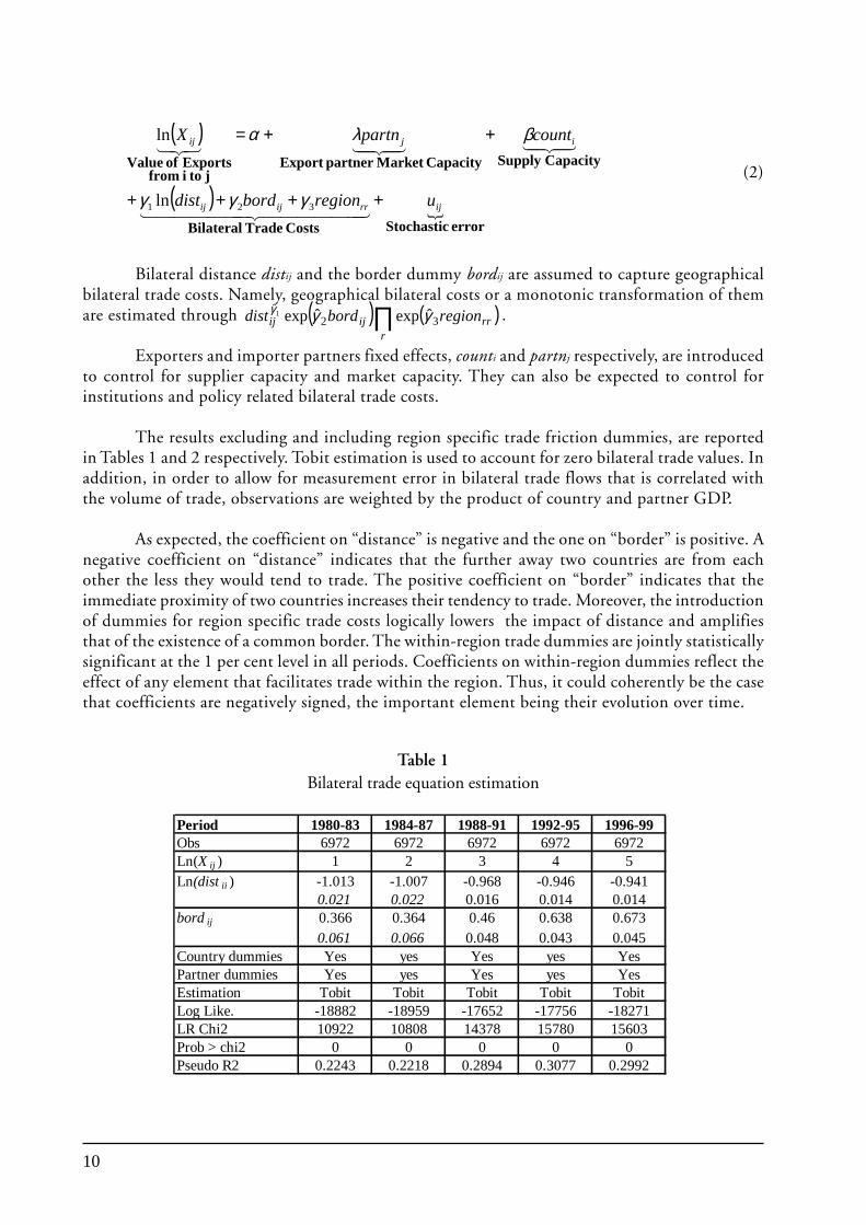
Bilateral distance distij and the border dummy bordij are assumed to capture geographicalbilateral trade costs. Namely, geographical bilateral costs or a monotonic transformation of themare estimated through ( ) ( )rr

rijij regionborddist 32

ˆ ˆexpˆexp1 γγγ ∏ .

Exporters and importer partners fixed effects, counti and partnj respectively, are introducedto control for supplier capacity and market capacity. They can also be expected to control forinstitutions and policy related bilateral trade costs.

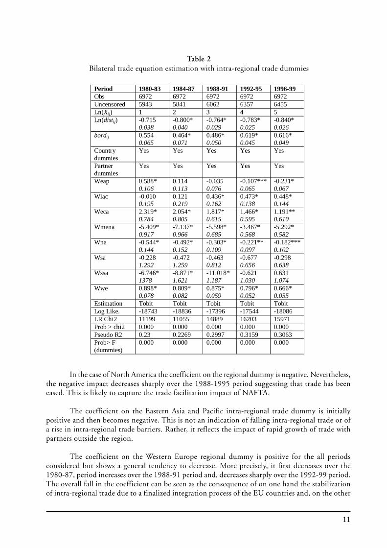
The results excluding and including region specific trade friction dummies, are reportedin Tables 1 and 2 respectively. Tobit estimation is used to account for zero bilateral trade values. Inaddition, in order to allow for measurement error in bilateral trade flows that is correlated withthe volume of trade, observations are weighted by the product of country and partner GDP.

As expected, the coefficient on “distance” is negative and the one on “border” is positive. Anegative coefficient on “distance” indicates that the further away two countries are from eachother the less they would tend to trade. The positive coefficient on “border” indicates that theimmediate proximity of two countries increases their tendency to trade. Moreover, the introductionof dummies for region specific trade costs logically lowers the impact of distance and amplifiesthat of the existence of a common border. The within-region trade dummies are jointly statisticallysignificant at the 1 per cent level in all periods. Coefficients on within-region dummies reflect theeffect of any element that facilitates trade within the region. Thus, it could coherently be the casethat coefficients are negatively signed, the important element being their evolution over time.

( )

( )�

error StochasticCosts Trade Bilateral

Capacity SupplyCapacityMarket partner Export j to i from

Exports of Value

ijrrijij

ijij

uregionborddist

countpartnX

++++

++=

��

��

321 ln

ln

γγγ

βλα

Table 1Bilateral trade equation estimation

Period 1980-83 1984-87 1988-91 1992-95 1996-99Obs 6972 6972 6972 6972 6972Ln(X ij ) 1 2 3 4 5Ln(dist ij ) -1.013 -1.007 -0.968 -0.946 -0.941

0.021 0.022 0.016 0.014 0.014bord ij 0.366 0.364 0.46 0.638 0.673

0.061 0.066 0.048 0.043 0.045Country dummies Yes yes Yes yes YesPartner dummies Yes yes Yes yes YesEstimation Tobit Tobit Tobit Tobit TobitLog Like. -18882 -18959 -17652 -17756 -18271LR Chi2 10922 10808 14378 15780 15603Prob > chi2 0 0 0 0 0Pseudo R2 0.2243 0.2218 0.2894 0.3077 0.2992

11

In the case of North America the coefficient on the regional dummy is negative. Nevertheless,the negative impact decreases sharply over the 1988-1995 period suggesting that trade has beeneased. This is likely to capture the trade facilitation impact of NAFTA.

The coefficient on the Eastern Asia and Pacific intra-regional trade dummy is initiallypositive and then becomes negative. This is not an indication of falling intra-regional trade or ofa rise in intra-regional trade barriers. Rather, it reflects the impact of rapid growth of trade withpartners outside the region.

The coefficient on the Western Europe regional dummy is positive for the all periodsconsidered but shows a general tendency to decrease. More precisely, it first decreases over the1980-87, period increases over the 1988-91 period and, decreases sharply over the 1992-99 period.The overall fall in the coefficient can be seen as the consequence of on one hand the stabilizationof intra-regional trade due to a finalized integration process of the EU countries and, on the other

Period 1980-83 1984-87 1988-91 1992-95 1996-99 Obs 6972 6972 6972 6972 6972 Uncensored 5943 5841 6062 6357 6455 Ln(Xij) 1 2 3 4 5 Ln(distij) -0.715

0.038 -0.800* 0.040

-0.764* 0.029

-0.783* 0.025

-0.840* 0.026

bordij 0.554 0.065

0.464* 0.071

0.486* 0.050

0.619* 0.045

0.616* 0.049

Country dummies

Yes Yes Yes Yes Yes

Partner dummies

Yes Yes Yes Yes Yes

Weap 0.588* 0.106

0.114 0.113

-0.035 0.076

-0.107*** 0.065

-0.231* 0.067

Wlac -0.010 0.195

0.121 0.219

0.436* 0.162

0.473* 0.138

0.448* 0.144

Weca 2.319* 0.784

2.054* 0.805

1.817* 0.615

1.466* 0.595

1.191** 0.610

Wmena -5.409* 0.917

-7.137* 0.966

-5.598* 0.685

-3.467* 0.568

-5.292* 0.582

Wna -0.544* 0.144

-0.492* 0.152

-0.303* 0.109

-0.221** 0.097

-0.182*** 0.102

Wsa -0.228 1.292

-0.472 1.259

-0.463 0.812

-0.677 0.656

-0.298 0.638

Wssa -6.746* 1378

-8.871* 1.621

-11.018* 1.187

-0.621 1.030

0.631 1.074

Wwe 0.898* 0.078

0.809* 0.082

0.875* 0.059

0.796* 0.052

0.666* 0.055

Estimation Tobit Tobit Tobit Tobit Tobit Log Like. -18743 -18836 -17396 -17544 -18086 LR Chi2 11199 11055 14889 16203 15971 Prob > chi2 0.000 0.000 0.000 0.000 0.000 Pseudo R2 0.23 0.2269 0.2997 0.3159 0.3063 Prob> F (dummies)

0.000 0.000 0.000 0.000 0.000

Table 2Bilateral trade equation estimation with intra-regional trade dummies

12

hand of the growing relative importance of trade with countries outside the region. Part of the fallin the value of the coefficient observed for the 1992-99 period could also be explained by theapparent fall in intra-regional trade due to the introduction in January 1993 of a new system forcollecting statistics on trade between EU member States INTRASTAT.3

The same downward tendency is observed for Eastern European countries with the sharpestdecrease in the coefficient during the period that includes the fall of the Berlin wall. Regressionshave also been run with a regional dummy that includes all Western and Eastern European countries.The coefficient on the dummy and its significance both increase, although moderately, over time.This is likely to capture the process of European enlargement and integration and confirms thearguments just mentioned.

Coefficients on the sub-Saharan region dummy are negative and large compared to otherregions’ coefficients when significant. This very much reflects poor infrastructures and poorgeographical factors. For the last two periods, the coefficient turns to be non-significant. Thisresult might reflect an improvement in the trade conditions compared to those prevailing in the1980s. However, it could also reflect the fact that trade integration has occurred more at a sub-regional level than at a regional level. Trade has intensified radically between countries belongingto the Southern African Development Community over the 1980-99 period compared to otherregional economic communities. The share of intra-trade in regional trade jumped from 54 percent in 1980 to 79 per cent in 1999.4 An upward trend is observed for most of the regionalcountry groups, which again could indicate that trade has become more sub-region specific thanregion specific.

The Middle East and North Africa dummy has a negative coefficient, which increases anddecreases alternatively. Together with its relatively high value, this is likely to reflect the negativeimpact of conflicts within the region and the volatility of prices of oil exports to countries outsidethe region.

(i) Foreign market Access

Following Redding and Venables (2004b) estimates obtained in the first stage of the analysisare used to construct supply capacity and foreign market access series. Because intra-regional tradedummies are not always significant, series for estimations do not include them. However, resultsobtained with series including intra regional trade dummies are discussed below.

The supply capacity estimate is given by the exponential of exporter country dummy timesits coefficient. That is

( )ii countSC β̂exp= (3)

Foreign market access estimate takes the form5

( ) ( )∑ ≠=

ji ijijji borddistpartnFMA 2ˆ êxpêxp 1 γλ γ

(3’)

3 See the GATT annual report 1994 for a brief description.4 See UNCTAD (2002), in particular Table 1.4.5 The version with intra regional dummies is

( ) ( ) ( )rrr

ji ijijji regionborddistimpFMA 32ˆ êxpêxpêxp 1 γγλ γ ∏∑ ≠

=

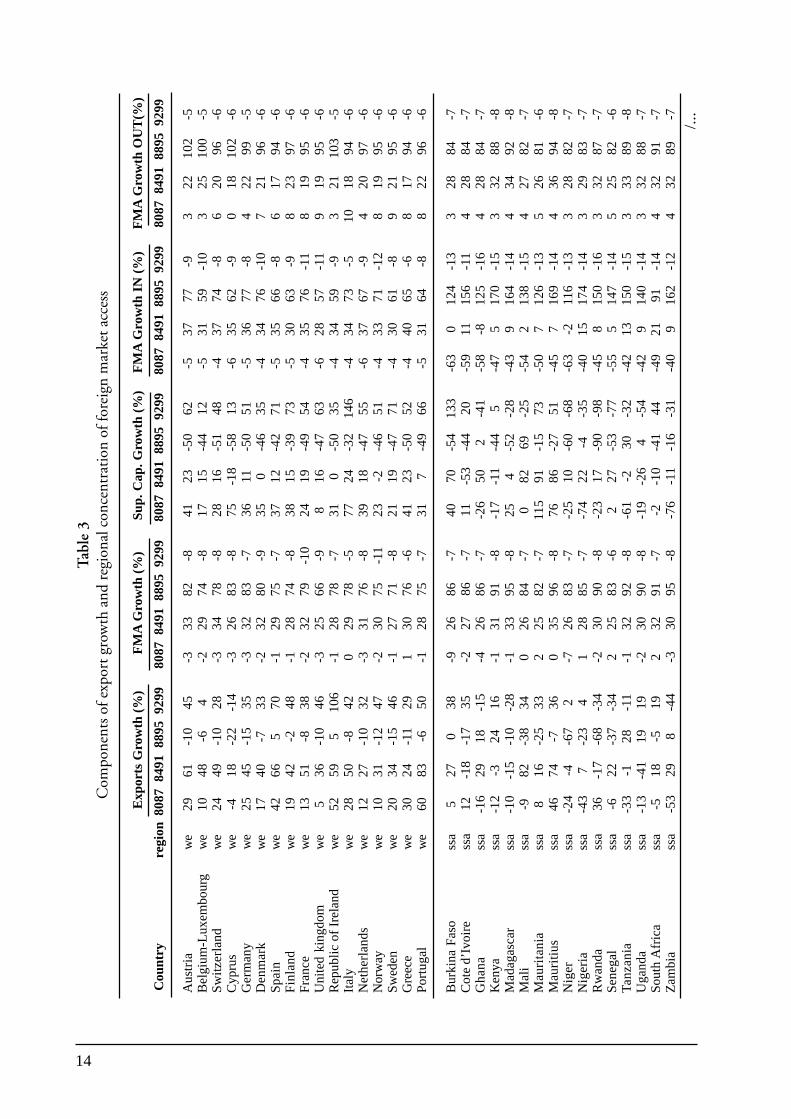
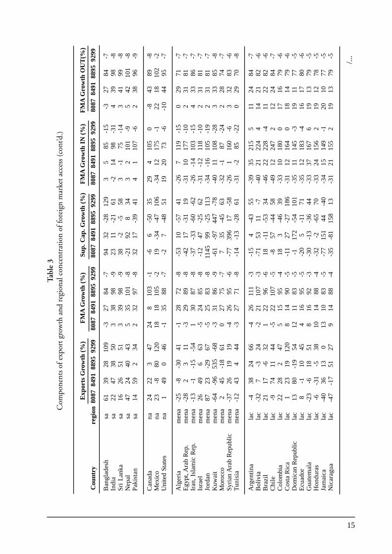
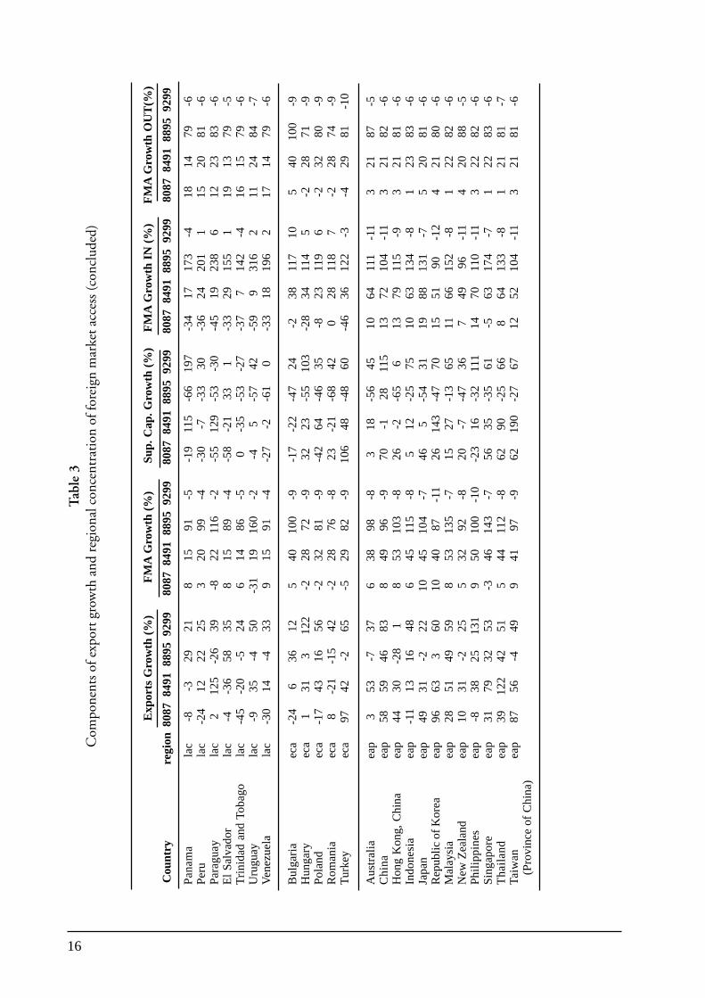
13

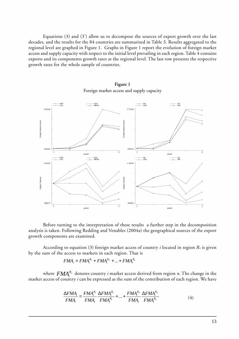
Equations (3) and (3’) allow us to decompose the sources of export growth over the lastdecades, and the results for the 84 countries are summarized in Table 3. Results aggregated to theregional level are graphed in Figure 1. Graphs in Figure 1 report the evolution of foreign marketaccess and supply capacity with respect to the initial level prevailing in each region. Table 4 containsexports and its components growth rates at the regional level. The last row presents the respectivegrowth rates for the whole sample of countries.

Before turning to the interpretation of these results a further step in the decompositionanalysis is taken. Following Redding and Venables (2004a) the geographical sources of the exportgrowth components are examined.

According to equation (3) foreign market access of country i located in region Rn is givenby the sum of the access to markets in each region. That is

nRi

Ri

Rii FMAFMAFMAFMA +++= ...21

where nRiFMA denotes country i market access derived from region n. The change in the

market access of country i can be expressed as the sum of the contribution of each region. We have

n

nn

Ri

Ri

i

Ri

Ri

Ri

i

Ri

i

i

FMA

FMA

FMA

FMA

FMA

FMA

FMA

FMA

FMA

FMA ∆++∆=∆...

1

11

(4)

For

eign

Mar

ket A

cces

s

period

EAP ECA LAC MENA

1 5

.976126

3.23148

For

eign

Mar

ket A

cces

s

period

NA SA SSA WE

1 5

.978753

2.71426

Sup

ply

Cap

acity

period

EAP ECA LAC MENA

1 5

.388274

1.63145

Sup

ply

Cap

acity

period

NA SA SSA WE

1 5

.459202

1.76416

Figure 1Foreign market access and supply capacity

14

Tab

le 3

Com

pone

nts

of e

xpor

t gro

wth

and

reg

iona

l con

cent

rati

on o

f for

eign

mar

ket a

cces

s

/...

Aus

tria

we

2961

-10

45-3

3382

-841

23-5

062

-537

77-9

322

102

-5B

elgi

um-L

uxem

bour

gw

e10

48-6

4-2

2974

-817

15-4

412

-531

59-1

03

2510

0-5

Sw

itze

rlan

dw

e24

49-1

028

-334

78-8

2816

-51

48-4

3774

-86

2096

-6C

ypru

sw

e-4

18-2

2-1

4-3

2683

-875

-18

-58

13-6

3562

-90

1810

2-6

Ger

man

yw

e25

45-1

535

-332

83-7

3611

-50

51-5

3677

-84

2299

-5D

enm

ark

we

1740

-733

-232

80-9

350

-46

35-4

3476

-10

721

96-6

Spa

inw

e42

665

70-1

2975

-737

12-4

271

-535

66-8

617

94-6

Fin

land

we

1942

-248

-128

74-8

3815

-39

73-5

3063

-98

2397

-6F

ranc

ew

e13

51-8

38-2

3279

-10

2419

-49

54-4

3576

-11

819

95-6

Uni

ted

king

dom

we

536

-10

46-3

2566

-98

16-4

763

-628

57-1

19

1995

-6R

epub

lic o

f Ir

elan

dw

e52

595

106

-128

78-7

310

-50

35-4

3459

-93

2110

3-5

Ital

yw

e28

50-8

420

2978

-577

24-3

214

6-4

3473

-510

1894

-6N

ethe

rlan

dsw

e12

27-1

032

-331

76-8

3918

-47

55-6

3767

-94

2097

-6N

orw

ayw

e10

31-1

247

-230

75-1

123

-2-4

651

-433

71-1

28

1995

-6Sw

eden

we

2034

-15

46-1

2771

-821

19-4

771

-430

61-8

921

95-6

Gre

ece

we

3024

-11

291

3076

-641

23-5

052

-440

65-6

817

94-6

Por

tuga

lw

e60

83-6

50-1

2875

-731

7-4

966

-531

64-8

822

96-6

Bur

kina

Fas

oss

a5

270

38-9

2686

-740

70-5

413

3-6

30

124

-13

328

84-7

Cot

e d’

Ivoi

ress

a12

-18

-17

35-2

2786

-711

-53

-44

20-5

911

156

-11

428

84-7

Gha

nass

a-1

629

18-1

5-4

2686

-7-2

650

2-4

1-5

8-8

125

-16

428

84-7

Ken

yass

a-1

2-3

2416

-131

91-8

-17

-11

-44

5-4

75

170

-15

332

88-8

Mad

agas

car

ssa

-10

-15

-10

-28

-133

95-8

254

-52

-28

-43

916

4-1

44

3492

-8M

ali

ssa

-982

-38

340

2684

-70

8269

-25

-54

213

8-1

54

2782

-7M

auri

tani

ass

a8

16-2

533

225

82-7

115

91-1

573

-50

712

6-1

35

2681

-6M

auri

tius

ssa

4674

-736

035

96-8

7686

-27

51-4

57

169

-14

436

94-8

Nig

erss

a-2

4-4

-67

2-7

2683

-7-2

510

-60

-68

-63

-211

6-1

33

2882

-7N

iger

iass

a-4

37

-23

41

2885

-7-7

422

-4-3

5-4

015

174

-14

329

83-7

Rw

anda

ssa

36-1

7-6

8-3

4-2

3090

-8-2

317

-90

-98

-45

815

0-1

63

3287

-7S

eneg

alss

a-6

22-3

7-3

42

2583

-62

27-5

3-7

7-5

55

147

-14

525

82-6

Tan

zani

ass

a-3

3-1

28-1

1-1

3292

-8-6

1-2

30-3

2-4

213

150

-15

333

89-8

Uga

nda

ssa

-13

-41

1919

-230

90-8

-19

-26

4-5

4-4

29

140

-14

332

88-7

Sout

h A

fric

ass

a-5

18-5

192

3291

-7-2

-10

-41

44-4

921

91-1

44

3291

-7Z

ambi

ass

a-5

329

8-4

4-3

3095

-8-7

6-1

1-1

6-3

1-4

09

162

-12

432

89-7

E

xpor

ts G

row

th (

%)

FM

A G

row

th (

%)

Sup.

Cap

. Gro

wth

(%

)F

MA

Gro

wth

IN

(%

)

FM

A G

row

th O

UT

(%)

Cou

ntry

regi

on80

8784

9188

9592

9980

8784

9188

9592

9980

8784

9188

9592

9980

8784

9188

9592

9980

8784

9188

9592

99

15

Tab

le 3

Com

pone

nts

of e

xpor

t gro

wth

and

reg

iona

l con

cent

rati

on o

f for

eign

mar

ket a

cces

s (c

ont’d

.)

/...

E

xpor

ts G

row

th (

%)

FM

A G

row

th (

%)

Sup.

Cap

. Gro

wth

(%

)F

MA

Gro

wth

IN

(%

)

FM

A G

row

th O

UT

(%)

Cou

ntry

regi

on80

8784

9188

9592

9980

8784

9188

9592

9980

8784

9188

9592

9980

8784

9188

9592

9980

8784

9188

9592

99

Ban

glad

esh

sa61

3928

109

-327

84-7

9432

-28

129

35

85-1

5-3

2784

-7In

dia

sa22

4738

503

3898

-923

11-2

161

-214

98-3

14

3998

-8Sr

i L

anka

sa16

2651

513

3998

-938

-2-5

583

-175

-14

341

99-8

Nep

alsa

4724

4043

535

101

-8-2

192

834

32

101

-95

4210

1-8

Pak

ista

nsa

1459

234

232

97-8

3217

-39

414

110

7-6

238

96-9

Can

ada

na24

223

4724

810

3-1

-66

-50

3529

410

50

-843

89-8

Mex

ico

na23

-880

120

1818

105

-219

-34

-47

106

-34

1217

5-1

2218

102

-2U

nite

d St

ates

na1

490

46-1

3588

-7-2

7-4

851

1920

73-6

-10

4495

-7

Alg

eria

men

a-2

5-8

-30

41-1

2872

-8-5

310

-57

41-2

67

119

-15

029

71-7

Egy

pt, A

rab

Rep

.m

ena

-28

23

11-3

2989

-8-4

217

-31

19-3

110

177

-10

231

81-7

Iran

, Is

lam

ic R

ep.

men

a-1

3-1

-15

-54

130

87-8

-37

-33

-60

-62

-26

-14

103

-15

433

86-7

Isra

elm

ena

2649

663

-524

85-8

-12

47-2

562

-31

-12

118

-10

231

81-7

Jord

anm

ena

8723

-29

67-5

2583

-811

4599

-25

113

-34

-16

105

-19

231

81-7

Kuw

ait

men

a-6

4-9

653

5-6

8-3

3186

-9-6

1-9

744

7-7

8-4

011

108

-28

333

85-8

Mor

occo

men

a2

45-1

861

027

75-7

735

-45

63-3

2-1

87-2

42

2874

-7Sy

rian

Ara

b R

epub

licm

ena

-37

2619

19-4

2695

-6-7

739

617

-58

-26

116

0-6

332

83-6

Tun

isia

men

a-1

243

444

-327

71-8

-14

-13

-28

61-3

1-2

85-2

20

2970

-8

Arg

enti

nala

c-4

3824

66-4

2611

1-3

-15

4-4

355

-39

3521

55

1124

84-7

Bol

ivia

lac

-32

7-3

24-2

2110

7-3

-71

5311

-7-4

021

224

414

2182

-6B

razi

lla

c21

17-6

321

2296

-618

-11

-53

34-4

622

228

-411

2282

-6C

hile

lac

-974

1144

-522

107

-5-8

57-4

458

-49

1224

72

1224

84-7

Col

ombi

ala

c22

282

475

1595

-418

3-4

639

-33

1018

00

1716

79-6

Cos

ta R

ica

lac

123

1912

08

1490

-5-1

127

-27

186

-31

1216

40

1814

79-6

Dom

ican

Rep

ublic

lac

1380

-19

5412

1183

-5-1

172

-54

101

-35

1114

5-3

1911

77-5

Ecu

ador

lac

8-1

1045

416

95-5

-20

5-1

171

-35

1218

3-4

1617

80-6

Gua

tem

ala

lac

-23

-618

518

1692

-3-3

0-1

3-3

644

-33

3716

76

1913

79-5

Hon

dura

sla

c-6

-31

-538

1014

88-4

-32

-2-6

570

-33

2415

62

1912

78-5

Jam

aica

lac

-40

3613

013

1083

-5-7

715

144

-40

-34

1514

9-1

2010

77-5

Nic

arag

uala

c-4

7-1

751

279

1488

-4-3

5-8

115

813

-31

2115

52

1913

79-5

16

Tab

le 3

Com

pone

nts

of e

xpor

t gro

wth

and

reg

iona

l con

cent

rati

on o

f for

eign

mar

ket a

cces

s (c

oncl

uded

)

Pan

ama

lac

-8-3

2921

815

91-5

-19

115

-66

197

-34

1717

3-4

1814

79-6

Per

ula

c-2

412

2225

320

99-4

-30

-7-3

330

-36

2420

11

1520

81-6

Par

agua

yla

c2

125

-26

39-8

2211

6-2

-55

129

-53

-30

-45

1923

86

1223

83-6

El

Salv

ador

lac

-4-3

658

358

1589

-4-5

8-2

133

1-3

329

155

119

1379

-5T

rini

dad

and

Toba

gola

c-4

5-2

0-5

246

1486

-50

-35

-53

-27

-37

714

2-4

1615

79-6

Uru

guay

lac

-935

-450

-31

1916

0-2

-45

-57

42-5

99

316

211

2484

-7V

enez

uela

lac

-30

14-4

339

1591

-4-2

7-2

-61

0-3

318

196

217

1479

-6

Bul

gari

aec

a-2

46

3612

540

100

-9-1

7-2

2-4

724

-238

117

105

4010

0-9

Hun

gary

eca

131

312

2-2

2872

-932

23-5

510

3-2

834

114

5-2

2871

-9P

olan

dec

a-1

743

1656

-232

81-9

-42

64-4

635

-823

119

6-2

3280

-9R

oman

iaec

a8

-21

-15

42-2

2876

-823

-21

-68

420

2811

87

-228

74-9

Tur

key

eca

9742

-265

-529

82-9

106

48-4

860

-46

3612

2-3

-429

81-1

0

Aus

tral

iaea

p3

53-7

376

3898

-83

18-5

645

1064

111

-11

321

87-5

Chi

naea

p58

5946

838

4996

-970

-128

115

1372

104

-11

321

82-6

Hon

g K

ong,

Chi

naea

p44

30-2

81

853

103

-826

-2-6

56

1379

115

-93

2181

-6In

done

sia

eap

-11

1316

486

4511

5-8

512

-25

7510

6313

4-8

123

83-6

Japa

nea

p49

31-2

2210

4510

4-7

465

-54

3119

8813

1-7

520

81-6

Rep

ublic

of

Kor

eaea

p96

633

6010

4087

-11

2614

3-4

770

1551

90-1

24

2180

-6M

alay

sia

eap

2851

4959

853

135

-715

27-1

365

1166

152

-81

2282

-6N

ew Z

eala

ndea

p10

31-2

255

3292

-820

-7-4

736

749

96-1

14

2088

-5P

hili

ppin

esea

p-8

3825

131

950

100

-10

-23

16-3

211

114

7011

0-1

13

2282

-6S

inga

pore

eap

3179

3253

-346

143

-756

35-3

561

-563

174

-71

2283

-6T

hail

and

eap

3912

242

515

4411

2-8

6290

-25

668

6413

3-8

121

81-7

Taiw

anea

p87

56-4

499

4197

-962

190

-27

6712

5210

4-1

13

2181

-6

(Pro

vinc

e of

Chi

na)

E

xpor

ts G

row

th (

%)

FM

A G

row

th (

%)

Sup.

Cap

. Gro

wth

(%

)F

MA

Gro

wth

IN

(%

)

FM

A G

row

th O

UT

(%)

Cou

ntry

regi

on80

8784

9188

9592

9980

8784

9188

9592

9980

8784

9188

9592

9980

8784

9188

9592

9980

8784

9188

9592

99

17

Equation (4) indicates that the contribution to country i foreign market access growth ofa given region is larger the larger the share of this region in country i foreign market access or thelarger the increase in market demand in the partner’s region.

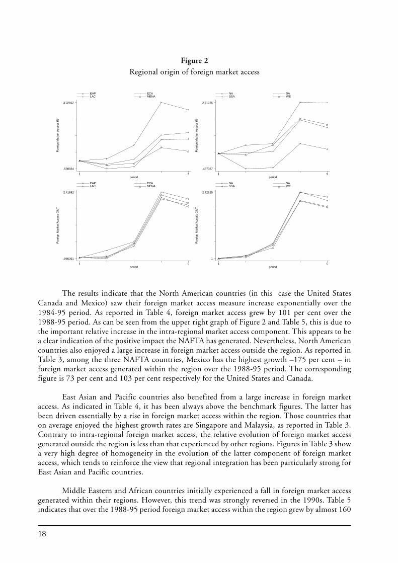
Graphs in Figure 2 show the evolution of foreign market access related to trade within theregion and across regions. Table 3 contains growth rates at the country level. Table 5 reports thelatter at the regional level. Benchmark values are presented in the last row.

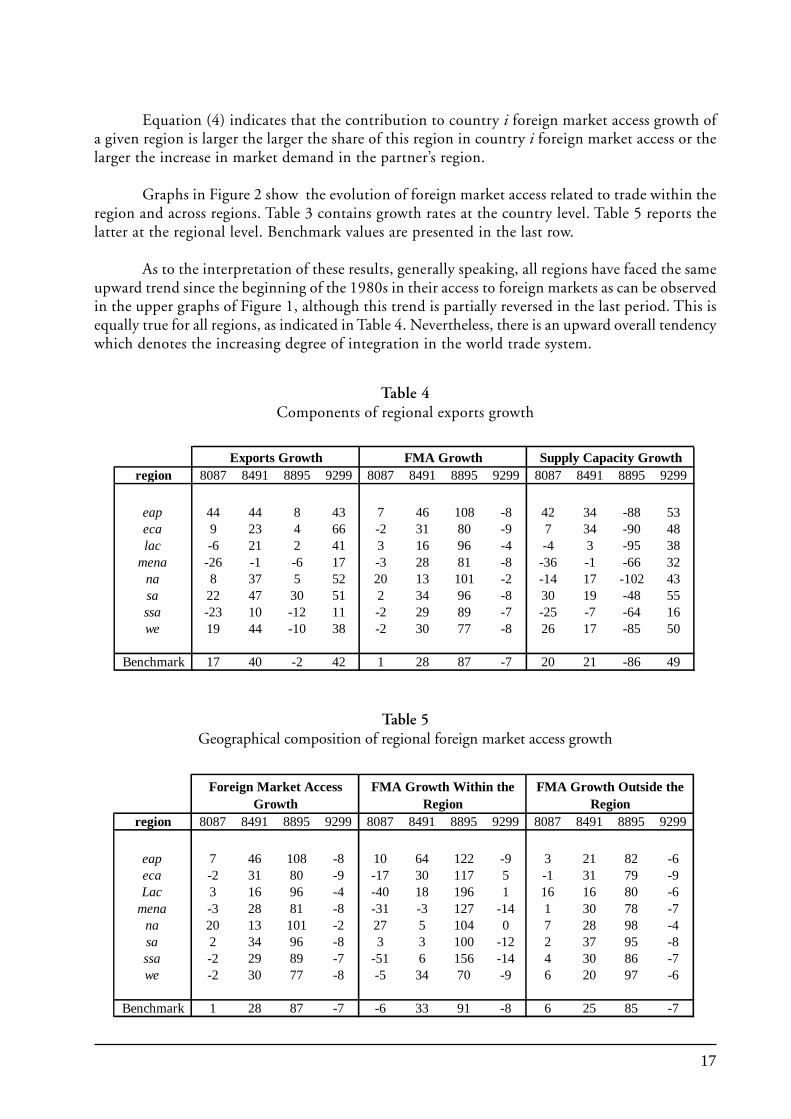
As to the interpretation of these results, generally speaking, all regions have faced the sameupward trend since the beginning of the 1980s in their access to foreign markets as can be observedin the upper graphs of Figure 1, although this trend is partially reversed in the last period. This isequally true for all regions, as indicated in Table 4. Nevertheless, there is an upward overall tendencywhich denotes the increasing degree of integration in the world trade system.

Table 4Components of regional exports growth

region 8087 8491 8895 9299 8087 8491 8895 9299 8087 8491 8895 9299

eap 44 44 8 43 7 46 108 -8 42 34 -88 53eca 9 23 4 66 -2 31 80 -9 7 34 -90 48lac -6 21 2 41 3 16 96 -4 -4 3 -95 38

mena -26 -1 -6 17 -3 28 81 -8 -36 -1 -66 32na 8 37 5 52 20 13 101 -2 -14 17 -102 43sa 22 47 30 51 2 34 96 -8 30 19 -48 55ssa -23 10 -12 11 -2 29 89 -7 -25 -7 -64 16we 19 44 -10 38 -2 30 77 -8 26 17 -85 50

Benchmark 17 40 -2 42 1 28 87 -7 20 21 -86 49

Exports Growth FMA Growth Supply Capacity Growth

region 8087 8491 8895 9299 8087 8491 8895 9299 8087 8491 8895 9299

eap 7 46 108 -8 10 64 122 -9 3 21 82 -6eca -2 31 80 -9 -17 30 117 5 -1 31 79 -9Lac 3 16 96 -4 -40 18 196 1 16 16 80 -6

mena -3 28 81 -8 -31 -3 127 -14 1 30 78 -7na 20 13 101 -2 27 5 104 0 7 28 98 -4sa 2 34 96 -8 3 3 100 -12 2 37 95 -8ssa -2 29 89 -7 -51 6 156 -14 4 30 86 -7we -2 30 77 -8 -5 34 70 -9 6 20 97 -6

Benchmark 1 28 87 -7 -6 33 91 -8 6 25 85 -7

Foreign Market Access Growth

FMA Growth Within the Region

FMA Growth Outside the Region

Table 5Geographical composition of regional foreign market access growth

18

The results indicate that the North American countries (in this case the United StatesCanada and Mexico) saw their foreign market access measure increase exponentially over the1984-95 period. As reported in Table 4, foreign market access grew by 101 per cent over the1988-95 period. As can be seen from the upper right graph of Figure 2 and Table 5, this is due tothe important relative increase in the intra-regional market access component. This appears to bea clear indication of the positive impact the NAFTA has generated. Nevertheless, North Americancountries also enjoyed a large increase in foreign market access outside the region. As reported inTable 3, among the three NAFTA countries, Mexico has the highest growth –175 per cent – inforeign market access generated within the region over the 1988-95 period. The correspondingfigure is 73 per cent and 103 per cent respectively for the United States and Canada.

East Asian and Pacific countries also benefited from a large increase in foreign marketaccess. As indicated in Table 4, it has been always above the benchmark figures. The latter hasbeen driven essentially by a rise in foreign market access within the region. Those countries thaton average enjoyed the highest growth rates are Singapore and Malaysia, as reported in Table 3.Contrary to intra-regional foreign market access, the relative evolution of foreign market accessgenerated outside the region is less than that experienced by other regions. Figures in Table 3 showa very high degree of homogeneity in the evolution of the latter component of foreign marketaccess, which tends to reinforce the view that regional integration has been particularly strong forEast Asian and Pacific countries.

Middle Eastern and African countries initially experienced a fall in foreign market accessgenerated within their regions. However, this trend was strongly reversed in the 1990s. Table 5indicates that over the 1988-95 period foreign market access within the region grew by almost 160

For

eign

Mar

ket A

cces

s IN

period

EAP ECA LAC MENA

1 5

.598834

4.02662

For

eign

Mar

ket A

cces

s IN

period

NA SA SSA WE

1 5

.487027

2.71225

For

eign

Mar

ket A

cces

s O

UT

period

EAP ECA LAC MENA

1 5

.986391

2.41692F

orei

gn M

arke

t Acc

ess

OU

T

period

NA SA SSA WE

1 5

1

2.72625

Figure 2Regional origin of foreign market access

19

per cent for sub-Saharan countries and 130 per cent for Middle Eastern and North African countries.The highest growth rates are found for East African countries, which are also the best performersin terms of overall foreign market access growth. However, this general tendency was subsequentlyreversed.

A similar scenario holds for Latin American and Eastern European countries. Intra regionalforeign market access grew by almost 200 per cent in Latin America over the 1988-95 period. Asreported in Table 3, the higher rates of foreign market growth are found for countries belonging tothe MERCOSUR that was effectively launched at the beginning of the 1990s. The positive impactof this regional trade integration process is captured by above sample average growth rates of theintra-regional market access. The best performer in all foreign market access dimensions is Uruguay.Table 3 also shows that these countries also benefited from the high growth of market access fromoutside their region.

Foreign market access in South Asia is driven by both sources of access, although it appearedto be driven principally by extra regional market access in the second half of the 1980s. Intra-regional trade progression has also been positive although it tended to fall in the second half of the1990s as suggested by Table 5.

Foreign market access progression for Western European countries remains among thelowest in the period under observation. This reinforces the argument presented above that thosecountries were already well integrated at the beginning of this period and just followed the generaltrend. As shown in Table 5, growth rates for the region correspond almost exactly to those of thewhole sample. Moreover, Table 3 indicates that this result holds for all countries of the region.Such an homogeneous pattern is likely to reflect a strong degree of integration. Estimates alsoshow fast growth of market access generated outside the region over the 1988-95 period. Thisprobably reflects the EU’s growing web of regional agreements with Central and Eastern Europe,the Baltic States and the Euro-Med agreements.

Generally speaking, there is evidence of a positive impact of Regional Trade Agreementson trade between partner countries in particular over the 1984-95 period. Nevertheless, there isalso evidence of a strong positive contribution to foreign market access improvements and ofbetter access to non-neighbouring markets as indicated in the two lower panels of Figure 2,particularly in the 1984-95 period. For instance, the measure of foreign market access generatedoutside the region for Eastern European countries has increased considerably since the mid-1980sreflecting essentially the increasing integration of those countries to the Western European market.For all regions, an increasing upward trend in the mid-1980s can be observed, which correspondsto the beginning of an era of trade openness marked by the extensive unilateral liberalism underWorld Bank/International Monetary Fund programmes, the implementation of the results of theTokyo Round and, the growth of Regional Trade Agreements.

(ii) Supply capacity

The relative evolution of supply capacity is slightly more differentiated than that of foreignmarket access. There is no clear overall trend. However, all regions faced a sharp relative decreaseover the first half of the 1990s.

Asian countries show the largest relative increase in their supply capacity in the 1980s andthe lowest relative fall at the beginning of the 1990s. The best performers over the two decades

20

were Taiwan (Province of China) and Singapore. Figures reported in Table 3 indicate that thebulk of the growth in supply capacity occurred in the 1980s. The Chinese and the Philippines’supply capacities grew outstandingly in the 1992-99 period. Asian countries were also the bestperformers in relative terms over the two decades. There is an almost symmetric evolution betweenEast Asian foreign market access and supply capacity evolution. In particular, the fall in supplycapacity in the first half of the 1990s was offset by an upward shift in foreign market access.

The African and the Middle Eastern countries mostly experienced low or even negativegrowth in their supply capacities over the whole of the1990s as shown in Table 3. As a whole,growth rates turned positive only in the second half of the 1990s as shown in Table 4. This mayreflect to a large extent the negative impact of conflicts on infrastructure and related investment.

Table 4 indicates that North and Latin American countries experienced the largest relativefall in supply capacity over the 1988-95 period. Surprisingly enough, Table 3 reports that thelargest fall in supply capacity among North American countries was in the United States. However,such observations are theoretically coherent in the context of strong regional integration. As shownin Table 3, a decline in supply capacity was also experienced by most Latin American countries upto the first half of the 1990s. Export performance, if not negative, remained very low in thatperiod, most likely as a result of the impact of economic turmoil that characterized the region.

This is also true to some extent for Western European countries. They faced a severe fallin their supply capacity at the beginning of the 1990s after a decade of improvement. Nonetheless,the trend was reversed again in the second half of the 1990s. Table 3 indicates that except forCyprus and Norway in the 1984-1991 period all European countries moved together. Togetherwith negative export growth, the fall in supply capacity observed for the 1988-95 period couldreflect the negative impact that German reunification had on European economies.

(iii) Export Constraints

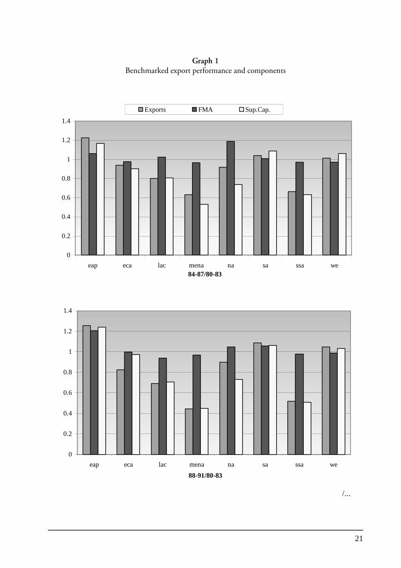
In order to identify export performance constraints more closely and to qualify the abovearguments, it is necessary to look at the evolution of performance and its components withrespect to the country sample values to be able to elicit the policy implications. Ratios of regionalvalues over sample values are computed for each period and then normalized to the ratio prevailingin the first period.6 This makes it possible to qualify the evolution of export performance for eachregion across periods and with respect to world export performance for each period. Exportperformance has been defined theoretically as the product of foreign market access and supplycapacity. That is, the exports ratio is equal to the product of the foreign market access and thesupply capacity ratios up to an error term related to estimation.

The Asia and Pacific regions are the only regions that have improved their exportperformance relative to the whole sample of countries in all periods (Graph 1). Both regions, andin particular South Asia and the Pacific, have experienced a relative improvement in their foreignmarket access across periods. However, their export performance is driven by an outstandingrelative improvement in their supply capacity. This is likely to reflect a policy orientation aiming

6 For instance the bar plotted in graph 1 for Exports 84-87/80-83 in region eap correspond to(Exportseap 84-87/ Exportssample 84-87)/ (Exportseap 80-83/ Exportssample 80-83).

21

0

0.2

0.4

0.6

0.8

1

1.2

1.4

eap eca lac mena na sa ssa we

88-91/80-83

0

0.2

0.4

0.6

0.8

1

1.2

1.4

eap eca lac mena na sa ssa we84-87/80-83

Exports FMA Sup.Cap.

Graph 1Benchmarked export performance and components

/...

22

0

0.2

0.4

0.6

0.8

1

1.2

1.4

1.6

eap eca lac mena na sa ssa we92-95/80-83

Exports FMA Sup.Cap.

0

0.2

0.4

0.6

0.8

1

1.2

1.4

1.6

1.8

eap eca lac mena na sa ssa we

96-99/80-83

Graph 1 (concluded)Benchmarked export performance and components

(Benchmark: ratio to 80-83 World Export Performance and Components)

23

to support and stimulate exporting firms’ productive capacities. This policy consisted not only inlevelling the playing field for exporters, but in boosting it in their favour by employinginterventionist policies7 such as the coordination of investment plans, directed credits and infantindustry protection.

Western European countries behaved in a similar manner as the country sample figures.Their export performance is led to some extent by supply capacity despite its relative deteriorationover the 1992-1995 period. In fact, foreign market access fell relatively in the last two periods.This deterioration with respect to sample levels indicates the strong degree of integration of theregion. This is confirmed by the fact that intra-regional trade has been constantly growing andtoday represents almost three quarters of the total trade of European countries.

The experience of Eastern European countries was similar to that of their Westerncounterparts, although supply capacity became a binding constraint element in the aftermath ofthe fall of the Berlin wall. All in all, their relative position remained stable over the two decades.

The experience of North American countries is to some extent puzzling, as it might havebeen expected to be quite similar to that of Western European countries. Instead, their relativesituation tended to deteriorate across periods, although only slightly, because of a relativedeterioration of supply capacity conditions. There is clear evidence that their foreign market accessposition improved, but their performance was constrained by a poor evolution of supply capacityconditions. On the other hand, theoretical insights predict that a negative relationship is likely toappear between the two dimensions. This is what is found when looking at regional growth rates.Supply capacity tends to decrease while foreign market access tends to increase.

With the advent of the NAFTA, some production has been shifted from the United Statesto northern Mexican regions. This could explain the fall in supply capacity in the United Statesover the 1988-95 period. Simultaneously, this new productive area bid up salaries, essentiallythose of skilled workers in Mexico, which may have reduced supply capacity in the country, aspredicted by the model previously presented.

The relative situations of the African and Middle Eastern countries’ tend to deteriorateover time. There is clear evidence that export performance is led by foreign market access. Thelatter appears to be stable with respect to sample levels, which indicates that those countries arelikely to face constraints in the development of supply capacity.

Regarding Latin American and Caribbean countries, foreign market access drives exportperformance. However, the latter fell in relative terms over the first two periods and stabilizedafterwards. Supply capacity tended to deteriorate over the whole period. As in the case of Africancountries this can be taken as an indication of the existence of supply capacity constraints.

Overall, a careful examination of the results derived from the estimation procedures outlinedabove indicates that supply capacity constraints seem to represent a significant barrier to thedevelopment of the export sector. This is true for both developed and developing countries.

7 See The World Bank (1993) for a comprehensive argumentation.

24

Over the two decades under consideration, export performance has been led essentially byan overall increase in both market access and supply capacity in Asian and Pacific countries. Thisis true also for European countries although on a much lower scale. North American countries’exports strongly benefited from NAFTA despite a poor evolution in their supply capacity, whichcan be seen as a by-product of strong production integration. Export performance in Latin American,Caribbean, African and Middle Eastern countries was mainly influenced by foreign market accessevolution. There is also evidence of an important impact of regional trade agreements within ageneral increasing world trade integration tendency.

(c) Sensitivity Analysis

In order to evaluate the robustness of thr results, foreign market access components wereestimated using a sample of 149 countries. While the main conclusions are unchanged, there arefew differences in the estimates of growth rates but, not enough to change the conclusions.

Five-year periods were also considered. Again, qualitative results remained similar.

Further, using estimates that include dummies for intra-regional trade, the results are verysimilar both in quantitative and qualitative terms. However, due to the loss of significance of thedummy for the sub-Saharan region in the last two periods, estimates for countries of that regionlose some coherence.

Finally, a different estimation strategy was adopted, based on a more structural approach.More precisely, the study estimates the following gravity model

( ) ( ) ( ) ( )ijjijiji

ijijij

uopenopenislislllockllock

borddistX

++++++

+++++=

876543

21ji lnGDPlnGDPlnln

γγγγγγγγβλα

where GDPi and GDPj stand for country and partner GDP, respectively. They represent countryi supply capacity and partner j demand capacity respectively. Trade costs estimates are augmentedby a series of indicators. Dummies llocki and llockj indicate whether the country and the partnerrespectively are landlocked. Dummies isli and islj indicate whether the country and the partnerrespectively are islands. Indicators openi and openj correspond to the Sachs and Warner (1995)composite index.8

In this case the results remain similar from a qualitative point of view on aggregate, butshow some large differences across time. Foreign market access series obtained with the twoestimation strategies are highly correlated. However, R-squared values are lower in the secondapproach than in the first. This implies that estimated values of exports could appear to besignificantly different from real ones. As a consequence, the estimated series for foreign marketaccess may not be fully consistent with real export series.

8 The latter establishes according to five criteria – tariffs, quotas coverage, black market premium, social organizationand the existence of export marketing boards – whether a country runs or not an open trade policy.

25

This chapter attempts to clarify further the key components of supply capacity. It alsoattempts to account for non-linearities in the process of development of the external sector. Forthat reason econometric techniques able to deal with unobservable heterogeneity are used.

(a) An Extended Theoretical Framework

In the theoretical framework presented previously, supply capacity, as indicated in equation(4’), is a function of the size of the export sector measured by the number of varieties produced,producer prices and internal transport costs. A country’s GDP and its population are measures ofcountry size. Country size reflects the home market and is likely to be linked to the size of theexternal sector and export prices. The latter directly reflect comparative costs of exporting whichare also linked for instance to institutions or real exchange rates.

Supply capacity is also expected to depend on foreign market access. Better access tointernational markets would imply higher expected returns from export activities. As a consequence,the external sector would tend to expand with some impact on supply capacity. The relation betweenforeign market access and supply capacity is thus made endogenous. In order to qualify theconsequences of such a relationship, some general equilibrium features needs to be added to thetheoretical framework.

Redding and Venables (2004a) consider a production possibility frontier between exportsand other goods. In that context the model predicts a negative relationship between foreign marketaccess and supply capacity. High levels of foreign market access are expected to be associated witha less than proportional increase in exports and a lower level of supply capacity. An expansion ofthe export sector increases the cost of factors by increasing demand pressure and thus leads tohigher producer prices, which are negatively related to supply capacity. However, the sign of therelationship could be arguable. Better foreign market access could also draw production resourcesfrom abroad via foreign direct investment or labour migration. In that case, factor demand pressurecould be eased and the sign of the relationship could become uncertain at least to a certain extent.

Empirically, if the first effect (factor prices) dominates the second (factors supply) an estimateof the elasticity of export performance with respect to foreign market access, which is less than onewould be obtained. In other words, export performance would be expected to grow less thanproportionally than foreign market access. On the contrary, if the elasticity of export performancewith respect to foreign market access is greater than one, then exports would growth proportionallymore than foreign market access.

(b) The Data

Sources of data on the variables described in the next chapter are presented in Appendix A.Data availability is a major constraint and in order to keep analytical relevance and statisticalcoherence, empirical investigations are run for the three 4-year periods covering 1988-1999. In

III. EXPORT PERFORMANCE AND ITS DETERMINANTS

26

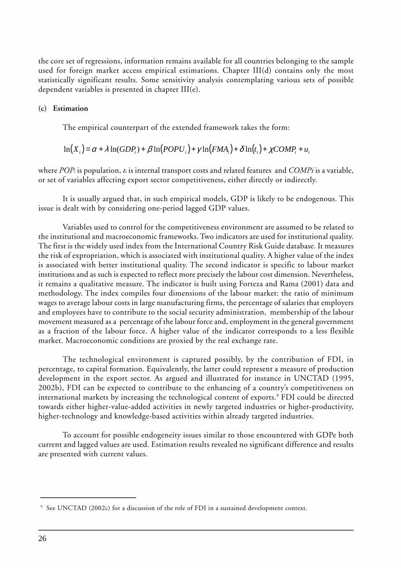
the core set of regressions, information remains available for all countries belonging to the sampleused for foreign market access empirical estimations. Chapter III(d) contains only the moststatistically significant results. Some sensitivity analysis contemplating various sets of possibledependent variables is presented in chapter III(e).

(c) Estimation

The empirical counterpart of the extended framework takes the form:

( ) ( ) ( ) ( ) iiiiiii uCOMPtFMAPOPUGDPX ++++++= χδγβλα lnlnln)ln(ln

where POPi is population, ti is internal transport costs and related features and COMPi is a variable,or set of variables affecting export sector competitiveness, either directly or indirectly.

It is usually argued that, in such empirical models, GDP is likely to be endogenous. Thisissue is dealt with by considering one-period lagged GDP values.

Variables used to control for the competitiveness environment are assumed to be related tothe institutional and macroeconomic frameworks. Two indicators are used for institutional quality.The first is the widely used index from the International Country Risk Guide database. It measuresthe risk of expropriation, which is associated with institutional quality. A higher value of the indexis associated with better institutional quality. The second indicator is specific to labour marketinstitutions and as such is expected to reflect more precisely the labour cost dimension. Nevertheless,it remains a qualitative measure. The indicator is built using Forteza and Rama (2001) data andmethodology. The index compiles four dimensions of the labour market: the ratio of minimumwages to average labour costs in large manufacturing firms, the percentage of salaries that employersand employees have to contribute to the social security administration, membership of the labourmovement measured as a percentage of the labour force and, employment in the general governmentas a fraction of the labour force. A higher value of the indicator corresponds to a less flexiblemarket. Macroeconomic conditions are proxied by the real exchange rate.

The technological environment is captured possibly, by the contribution of FDI, inpercentage, to capital formation. Equivalently, the latter could represent a measure of productiondevelopment in the export sector. As argued and illustrated for instance in UNCTAD (1995,2002b), FDI can be expected to contribute to the enhancing of a country’s competitiveness oninternational markets by increasing the technological content of exports.9 FDI could be directedtowards either higher-value-added activities in newly targeted industries or higher-productivity,higher-technology and knowledge-based activities within already targeted industries.

To account for possible endogeneity issues similar to those encountered with GDPe bothcurrent and lagged values are used. Estimation results revealed no significant difference and resultsare presented with current values.

9 See UNCTAD (2002c) for a discussion of the role of FDI in a sustained development context.

27

Internal transport frictions are introduced via the percentage of paved roads in total roadnetworks. Transport structure variables are likely to capture internal transport frictions more preciselythan exclusively geographical variables. In order to deal with possible endogeneity issues (thedevelopment of infrastructures could be fostered by higher export growth) again current and laggedvalues are used. In the event, results are similar in both cases, and only regressions using currentvalues are presented.

Taking into consideration the fact that unobserved heterogeneity might play an importantrole in determining export performance, but the set of available variables and indicators does notallow to control for it, quantile regression techniques are used,10 following the seminal work ofKoenker and Bassett (1978). Quantile techniques permit the study to allow for the existence ofunobservable heterogeneity not only through differences in the constant term, as is the case whenintroducing dummies, but also through differences in coefficients. The strength of the estimationrelies very much on the fact that these differences are obtained within the same sample and notacross samples. Quantile regression allows the characterization of an entire conditional distributionrather than only the mean of that distribution as in the case of standard OLS. In that sense,quantile regression is robust even in the presence of outliers, which is not the case for traditionalconditional mean estimation procedures.

In the present context, the distribution of the real value of countries’ total exports are dealtwith. Quantile regression allows the identification of different responses of exports value toFMA and supply capacity variables associated with different points on exports value conditionaldistribution. Nonetheless, quantile regression coefficients measure the determinants of exportperformance for under and over performing countries only in terms of export performance. Asestimation could modify the position of a given country, it may become hazardous to attributeexport performance determinants to over and under performing countries per se. Quantile regressionresults represent the basis for policy-oriented experiments aiming at qualifying possible exportperformance constraints.

(d) Results and Interpretation

Table 6 reports OLS regressions estimates and Tables 7 to 9 quantile regressions estimates.Standard errors reported in italics are computed from 1000 bootstrap samples.11 Five conditionalquantiles are considered: 10th (Q10), 25th (Q25), the median (Q50), 75th (Q75), and 90th (Q90).

The first observation is that some form of error heteroskedasticity seems to exist since theestimated coefficients vary with the quantiles. This confirms inference from OLS residuals plotting.Thus, quantile techniques seem to be appropriate for identifying the determinants of exportperformance at different levels of the latter. Again, the usefulness of quantile regressions rests firston the fact that they allow the identificationof possible elements that explain over- and under-performance with respect to mean. Second, put in a time perspective, it may give useful insightsinto the very process of export sector development.

10 A brief technical presentation of the quantile approach and its estimation techniques are presented in appendix C.Buchinsky (1998) provides a survey and general discussion.11 Almost identical results both in terms of coefficient values and standard errors values are obtained with 500bootstrap samples.

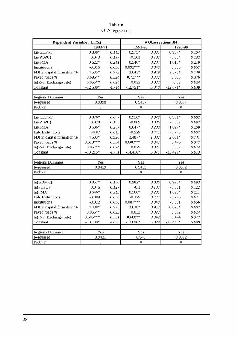
28

Table 6OLS regressions

Ln(GDPt-1) 0.838* 0.115 0.975* 0.085 0.967* 0.104Ln(POPU) 0.043 0.137 -0.101 0.103 -0.024 0.132Ln(FMA) 0.622* 0.211 0.546* 0.207 1.010* 0.210Institutions -0.016 0.058 0.092*** 0.049 0.003 0.057FDI in capital formation % 4.535* 0.972 3.643* 0.949 2.573* 0.748Paved roads % 0.696** 0.324 0.737** 0.332 0.533 0.376ln(Real Exchange rate) 0.055** 0.024 0.033 0.022 0.03 0.024Constant -12.530* 4.744 -12.751* 5.040 -22.871* 5.038

Regions DummiesR-squaredProb>F

Ln(GDPt-1) 0.876* 0.077 0.916* 0.079 0.991* 0.082Ln(POPU) 0.028 0.103 -0.009 0.086 -0.032 0.097Ln(FMA) 0.636* 0.207 0.647* 0.209 1.027* 0.208Lab. Institutions -0.87 0.645 -0.529 0.445 -0.775 0.607FDI in capital formation % 4.533* 0.920 3.487* 1.082 2.601* 0.741Paved roads % 0.619*** 0.334 0.600*** 0.343 0.476 0.377ln(Real Exchange rate) 0.057** 0.024 0.029 0.021 0.032 0.024Constant -13.215* 4.791 -14.418* 5.075 -23.429* 5.013


ln(GDPt-1) 0.857* 0.100 0.982* 0.086 0.990* 0.093ln(POPU) 0.046 0.127 -0.1 0.103 -0.031 0.122ln(FMA) 0.646* 0.213 0.560* 0.205 1.028* 0.211Lab. Institutions -0.889 0.656 -0.379 0.437 -0.776 0.621Institutions -0.022 0.056 0.087*** 0.049 -0.001 0.056FDI in capital formation % 4.438* 0.935 3.638* 0.952 0.025* 0.007Paved roads % 0.055** 0.023 0.033 0.022 0.032 0.024ln(Real Exchange rate) 0.605*** 0.321 0.688** 0.342 0.474 0.372Constant -13.139* 4.888 -13.090* 5.029 -23.440* 5.099


1988-91 1992-95 1996-99Dependent Variable : Ln(X) # Observations :84

0.946 0.93920 0 0

Yes Yes Yes0.9421

0

Yes Yes Yes0.9419 0.9433 0.9372

0 0

0 0

Yes Yes Yes0.9398 0.9457 0.9377

0

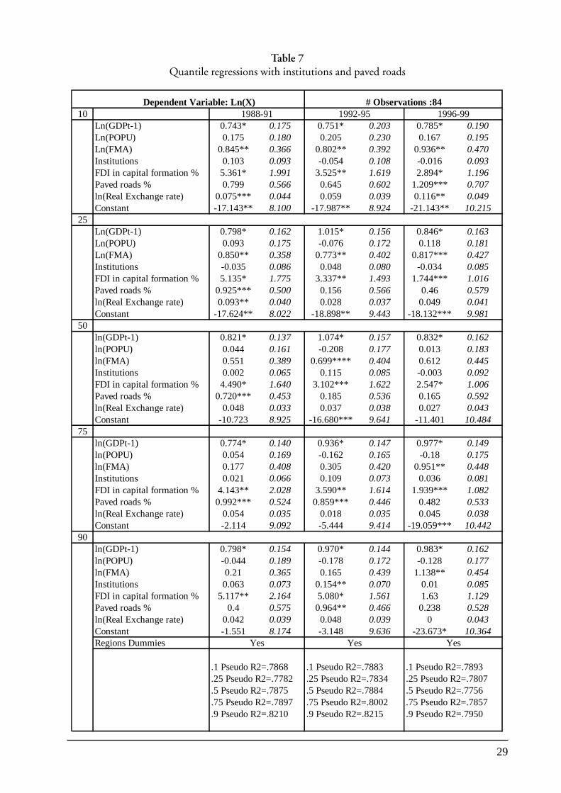
29

10Ln(GDPt-1) 0.743* 0.175 0.751* 0.203 0.785* 0.190Ln(POPU) 0.175 0.180 0.205 0.230 0.167 0.195Ln(FMA) 0.845** 0.366 0.802** 0.392 0.936** 0.470Institutions 0.103 0.093 -0.054 0.108 -0.016 0.093FDI in capital formation % 5.361* 1.991 3.525** 1.619 2.894* 1.196Paved roads % 0.799 0.566 0.645 0.602 1.209*** 0.707ln(Real Exchange rate) 0.075*** 0.044 0.059 0.039 0.116** 0.049Constant -17.143** 8.100 -17.987** 8.924 -21.143** 10.215

25Ln(GDPt-1) 0.798* 0.162 1.015* 0.156 0.846* 0.163Ln(POPU) 0.093 0.175 -0.076 0.172 0.118 0.181Ln(FMA) 0.850** 0.358 0.773** 0.402 0.817*** 0.427Institutions -0.035 0.086 0.048 0.080 -0.034 0.085FDI in capital formation % 5.135* 1.775 3.337** 1.493 1.744*** 1.016Paved roads % 0.925*** 0.500 0.156 0.566 0.46 0.579ln(Real Exchange rate) 0.093** 0.040 0.028 0.037 0.049 0.041Constant -17.624** 8.022 -18.898** 9.443 -18.132*** 9.981

50ln(GDPt-1) 0.821* 0.137 1.074* 0.157 0.832* 0.162ln(POPU) 0.044 0.161 -0.208 0.177 0.013 0.183ln(FMA) 0.551 0.389 0.699**** 0.404 0.612 0.445Institutions 0.002 0.065 0.115 0.085 -0.003 0.092FDI in capital formation % 4.490* 1.640 3.102*** 1.622 2.547* 1.006Paved roads % 0.720*** 0.453 0.185 0.536 0.165 0.592ln(Real Exchange rate) 0.048 0.033 0.037 0.038 0.027 0.043Constant -10.723 8.925 -16.680*** 9.641 -11.401 10.484

75ln(GDPt-1) 0.774* 0.140 0.936* 0.147 0.977* 0.149ln(POPU) 0.054 0.169 -0.162 0.165 -0.18 0.175ln(FMA) 0.177 0.408 0.305 0.420 0.951** 0.448Institutions 0.021 0.066 0.109 0.073 0.036 0.081FDI in capital formation % 4.143** 2.028 3.590** 1.614 1.939*** 1.082Paved roads % 0.992*** 0.524 0.859*** 0.446 0.482 0.533ln(Real Exchange rate) 0.054 0.035 0.018 0.035 0.045 0.038Constant -2.114 9.092 -5.444 9.414 -19.059*** 10.442

90ln(GDPt-1) 0.798* 0.154 0.970* 0.144 0.983* 0.162ln(POPU) -0.044 0.189 -0.178 0.172 -0.128 0.177ln(FMA) 0.21 0.365 0.165 0.439 1.138** 0.454Institutions 0.063 0.073 0.154** 0.070 0.01 0.085FDI in capital formation % 5.117** 2.164 5.080* 1.561 1.63 1.129Paved roads % 0.4 0.575 0.964** 0.466 0.238 0.528ln(Real Exchange rate) 0.042 0.039 0.048 0.039 0 0.043Constant -1.551 8.174 -3.148 9.636 -23.673* 10.364Regions Dummies

Dependent Variable: Ln(X)

.75 Pseudo R2=.7857

.9 Pseudo R2=.7950

# Observations :84

.1 Pseudo R2=.7893

.25 Pseudo R2=.7807

.5 Pseudo R2=.7756

.1 Pseudo R2=.7883

.25 Pseudo R2=.7834

.5 Pseudo R2=.7884

.75 Pseudo R2=.8002

.9 Pseudo R2=.8215

Yes Yes Yes

.1 Pseudo R2=.7868

.25 Pseudo R2=.7782

.5 Pseudo R2=.7875

.75 Pseudo R2=.7897

.9 Pseudo R2=.8210

1988-91 1992-95 1996-99

Table 7Quantile regressions with institutions and paved roads

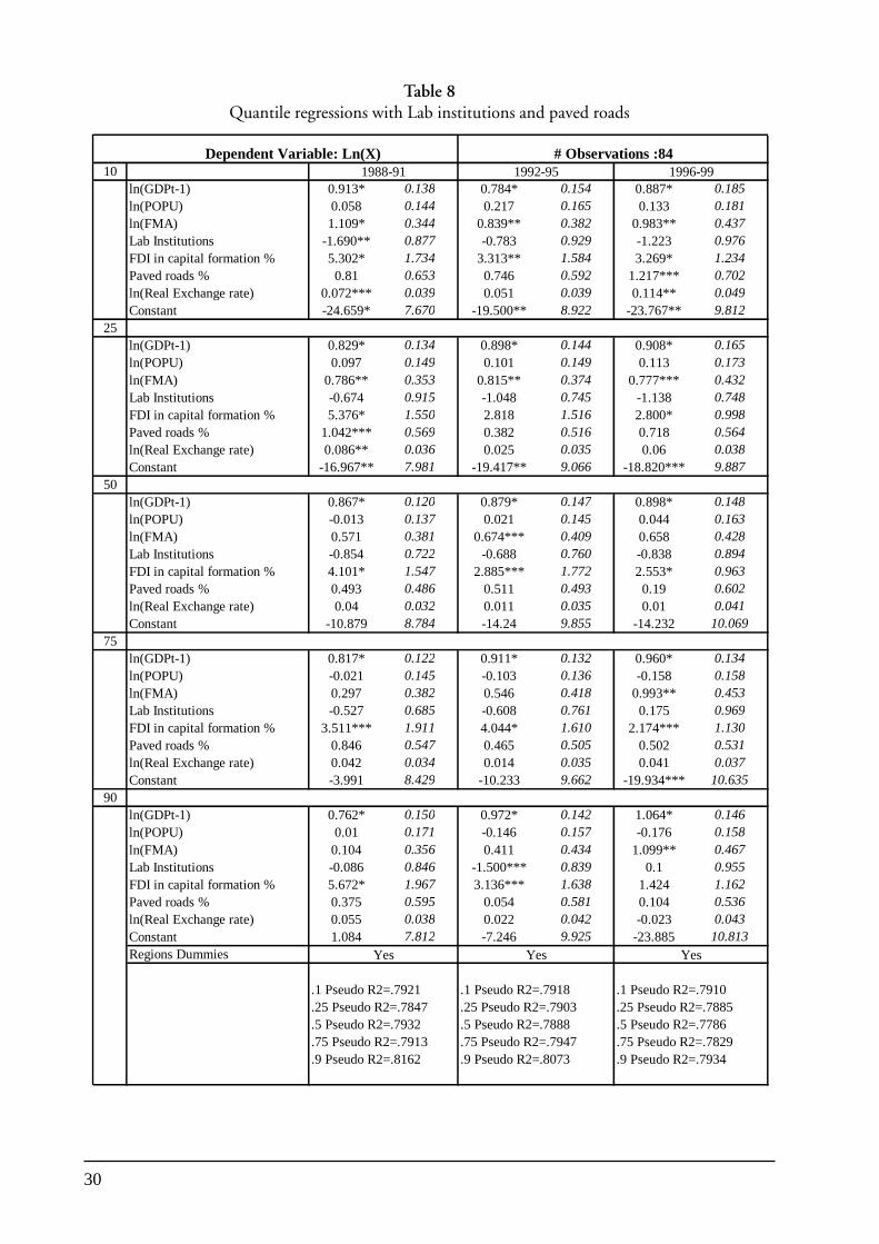
30

Table 8Quantile regressions with Lab institutions and paved roads

10ln(GDPt-1) 0.913* 0.138 0.784* 0.154 0.887* 0.185ln(POPU) 0.058 0.144 0.217 0.165 0.133 0.181ln(FMA) 1.109* 0.344 0.839** 0.382 0.983** 0.437Lab Institutions -1.690** 0.877 -0.783 0.929 -1.223 0.976FDI in capital formation % 5.302* 1.734 3.313** 1.584 3.269* 1.234Paved roads % 0.81 0.653 0.746 0.592 1.217*** 0.702ln(Real Exchange rate) 0.072*** 0.039 0.051 0.039 0.114** 0.049Constant -24.659* 7.670 -19.500** 8.922 -23.767** 9.812

25ln(GDPt-1) 0.829* 0.134 0.898* 0.144 0.908* 0.165ln(POPU) 0.097 0.149 0.101 0.149 0.113 0.173ln(FMA) 0.786** 0.353 0.815** 0.374 0.777*** 0.432Lab Institutions -0.674 0.915 -1.048 0.745 -1.138 0.748FDI in capital formation % 5.376* 1.550 2.818 1.516 2.800* 0.998Paved roads % 1.042*** 0.569 0.382 0.516 0.718 0.564ln(Real Exchange rate) 0.086** 0.036 0.025 0.035 0.06 0.038Constant -16.967** 7.981 -19.417** 9.066 -18.820*** 9.887

50ln(GDPt-1) 0.867* 0.120 0.879* 0.147 0.898* 0.148ln(POPU) -0.013 0.137 0.021 0.145 0.044 0.163ln(FMA) 0.571 0.381 0.674*** 0.409 0.658 0.428Lab Institutions -0.854 0.722 -0.688 0.760 -0.838 0.894FDI in capital formation % 4.101* 1.547 2.885*** 1.772 2.553* 0.963Paved roads % 0.493 0.486 0.511 0.493 0.19 0.602ln(Real Exchange rate) 0.04 0.032 0.011 0.035 0.01 0.041Constant -10.879 8.784 -14.24 9.855 -14.232 10.069

75ln(GDPt-1) 0.817* 0.122 0.911* 0.132 0.960* 0.134ln(POPU) -0.021 0.145 -0.103 0.136 -0.158 0.158ln(FMA) 0.297 0.382 0.546 0.418 0.993** 0.453Lab Institutions -0.527 0.685 -0.608 0.761 0.175 0.969FDI in capital formation % 3.511*** 1.911 4.044* 1.610 2.174*** 1.130Paved roads % 0.846 0.547 0.465 0.505 0.502 0.531ln(Real Exchange rate) 0.042 0.034 0.014 0.035 0.041 0.037Constant -3.991 8.429 -10.233 9.662 -19.934*** 10.635

90ln(GDPt-1) 0.762* 0.150 0.972* 0.142 1.064* 0.146ln(POPU) 0.01 0.171 -0.146 0.157 -0.176 0.158ln(FMA) 0.104 0.356 0.411 0.434 1.099** 0.467Lab Institutions -0.086 0.846 -1.500*** 0.839 0.1 0.955FDI in capital formation % 5.672* 1.967 3.136*** 1.638 1.424 1.162Paved roads % 0.375 0.595 0.054 0.581 0.104 0.536ln(Real Exchange rate) 0.055 0.038 0.022 0.042 -0.023 0.043Constant 1.084 7.812 -7.246 9.925 -23.885 10.813Regions Dummies

# Observations :84Dependent Variable: Ln(X)

.1 Pseudo R2=.7910.1 Pseudo R2=.7918

.5 Pseudo R2=.7888

.75 Pseudo R2=.7947

.9 Pseudo R2=.8073.75 Pseudo R2=.7829.9 Pseudo R2=.7934

.5 Pseudo R2=.7786

Yes Yes

.25 Pseudo R2=.7903 .25 Pseudo R2=.7885

1996-99

.9 Pseudo R2=.8162

1988-91 1992-95

.1 Pseudo R2=.7921

.25 Pseudo R2=.7847

.5 Pseudo R2=.7932

.75 Pseudo R2=.7913

Yes

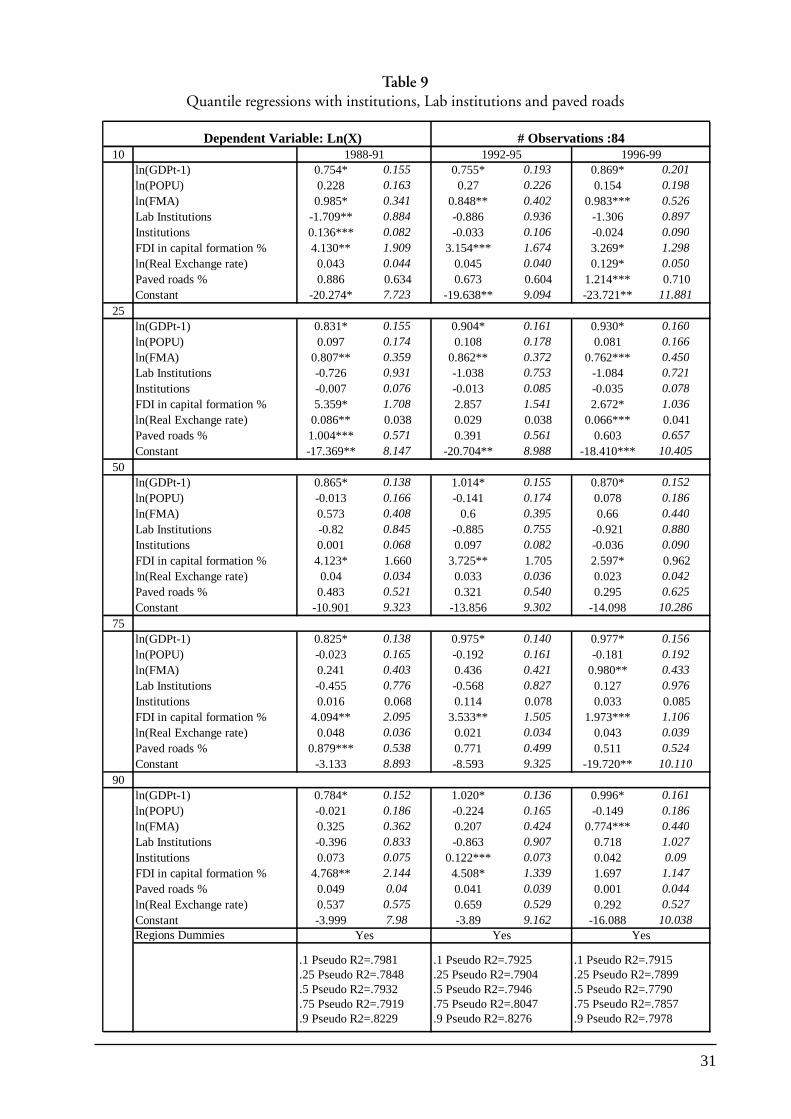
31

Table 9Quantile regressions with institutions, Lab institutions and paved roads

10ln(GDPt-1) 0.754* 0.155 0.755* 0.193 0.869* 0.201ln(POPU) 0.228 0.163 0.27 0.226 0.154 0.198ln(FMA) 0.985* 0.341 0.848** 0.402 0.983*** 0.526Lab Institutions -1.709** 0.884 -0.886 0.936 -1.306 0.897Institutions 0.136*** 0.082 -0.033 0.106 -0.024 0.090FDI in capital formation % 4.130** 1.909 3.154*** 1.674 3.269* 1.298ln(Real Exchange rate) 0.043 0.044 0.045 0.040 0.129* 0.050Paved roads % 0.886 0.634 0.673 0.604 1.214*** 0.710Constant -20.274* 7.723 -19.638** 9.094 -23.721** 11.881

25ln(GDPt-1) 0.831* 0.155 0.904* 0.161 0.930* 0.160ln(POPU) 0.097 0.174 0.108 0.178 0.081 0.166ln(FMA) 0.807** 0.359 0.862** 0.372 0.762*** 0.450Lab Institutions -0.726 0.931 -1.038 0.753 -1.084 0.721Institutions -0.007 0.076 -0.013 0.085 -0.035 0.078FDI in capital formation % 5.359* 1.708 2.857 1.541 2.672* 1.036ln(Real Exchange rate) 0.086** 0.038 0.029 0.038 0.066*** 0.041Paved roads % 1.004*** 0.571 0.391 0.561 0.603 0.657Constant -17.369** 8.147 -20.704** 8.988 -18.410*** 10.405

50ln(GDPt-1) 0.865* 0.138 1.014* 0.155 0.870* 0.152ln(POPU) -0.013 0.166 -0.141 0.174 0.078 0.186ln(FMA) 0.573 0.408 0.6 0.395 0.66 0.440Lab Institutions -0.82 0.845 -0.885 0.755 -0.921 0.880Institutions 0.001 0.068 0.097 0.082 -0.036 0.090FDI in capital formation % 4.123* 1.660 3.725** 1.705 2.597* 0.962ln(Real Exchange rate) 0.04 0.034 0.033 0.036 0.023 0.042Paved roads % 0.483 0.521 0.321 0.540 0.295 0.625Constant -10.901 9.323 -13.856 9.302 -14.098 10.286

75ln(GDPt-1) 0.825* 0.138 0.975* 0.140 0.977* 0.156ln(POPU) -0.023 0.165 -0.192 0.161 -0.181 0.192ln(FMA) 0.241 0.403 0.436 0.421 0.980** 0.433Lab Institutions -0.455 0.776 -0.568 0.827 0.127 0.976Institutions 0.016 0.068 0.114 0.078 0.033 0.085FDI in capital formation % 4.094** 2.095 3.533** 1.505 1.973*** 1.106ln(Real Exchange rate) 0.048 0.036 0.021 0.034 0.043 0.039Paved roads % 0.879*** 0.538 0.771 0.499 0.511 0.524Constant -3.133 8.893 -8.593 9.325 -19.720** 10.110

90ln(GDPt-1) 0.784* 0.152 1.020* 0.136 0.996* 0.161ln(POPU) -0.021 0.186 -0.224 0.165 -0.149 0.186ln(FMA) 0.325 0.362 0.207 0.424 0.774*** 0.440Lab Institutions -0.396 0.833 -0.863 0.907 0.718 1.027Institutions 0.073 0.075 0.122*** 0.073 0.042 0.09FDI in capital formation % 4.768** 2.144 4.508* 1.339 1.697 1.147Paved roads % 0.049 0.04 0.041 0.039 0.001 0.044ln(Real Exchange rate) 0.537 0.575 0.659 0.529 0.292 0.527Constant -3.999 7.98 -3.89 9.162 -16.088 10.038Regions Dummies

Dependent Variable: Ln(X) # Observations :84

.1 Pseudo R2=.7981

.25 Pseudo R2=.7848

.5 Pseudo R2=.7932

.75 Pseudo R2=.7919

.9 Pseudo R2=.8229

Yes

.1 Pseudo R2=.7925

.25 Pseudo R2=.7904

.5 Pseudo R2=.7946

.75 Pseudo R2=.8047

.9 Pseudo R2=.8276

1988-91 1992-95 1996-99

.9 Pseudo R2=.7978

.1 Pseudo R2=.7915

.25 Pseudo R2=.7899

.5 Pseudo R2=.7790

.75 Pseudo R2=.7857

Yes Yes

32

(i) General Considerations

OLS estimates can be used as a benchmark. All coefficients are signed accordingly withtheoretical anticipations. All variables but labour institutions and ln(Population) appear to besignificant in some period. A positive relationship is always obtained between larger domesticoutput, better foreign market access and export performance. Transport infrastructures, measuredby the log of percentage of paved roads in the total road network, are likely to play a positive rolein determining export performance. A positive impact is also expected from FDI’s contribution tocapital formation. The log of the real exchange rate is found to have a positive impact in variousestimations. In other words, devaluation could be expected to stimulate exports. Better institutionsare also found to affect positively export performance. For the 1996-99 period only log of laggedGDP values, foreign market access and FDI contribution to capital formation are significant,although at the one per cent level.

In all estimation exercises using quantile techniques, the sign of coefficients when significantare in line with theoretical expectations and OLS estimates. Namely, higher GDP, better access toforeign markets, better institutions, a more competitive macroeconomic framework, less internaltransport frictions lead to higher export performance. Larger countries, with a larger population,are found to be less open. It was also found that FDI contribution to capital formation has apositive impact on export performance. This could first pinpoint the existence of technologicaltransfer from foreign companies and underline its positive impact on export performance.

(ii) GDP and Population

In all regressions, a recurrent result is the high significance of log GDP (lagged). Thisremains true across periods and across quantiles. The coefficient on the log of GDP is found to beless than one in a majority of cases. This reinforces the result that larger countries are less open.That is, larger countries will tend to export relatively less, although large countries are also thosewhose exports volumes tend to be larger. On the other hand, total population never proves to haveany significant effect on export performance. The quality of regressions does not vary dramaticallywith the institutional indicator used. In addition, general results remain qualitatively identical.However, coefficients on ln(GDP), ln(POPU) can vary importantly and generally not in amonotonic fashion. In general, for a given institutional indicator, qualitative results remain identical.

(iii) Internal Transport Frictions

The importance and significance of internal transport frictions varies from period to periodand from quantile to quantile. It appears that internal transport costs had a significant negativeimpact on export performance over the 1988-91 period among the weakest performers, that is, forthose in the first fourth of the distribution. Internal transport facilitation played an important roleacross all quantiles in the 1992-95 time frame. Its significance appears to increase substantially forthose exporters that are above the median of the sample. This remains true to a large extent overthe 1996-99 period although the percentage of paved roads is found to be significant at the 10 percent level for the first quantile only.

33

In other words, transport infrastructures are likely to play an important role at the earlystage of export sector development.12 The percentage of paved roads appears to be more significantand its impact to be larger in lower quantiles. As shown in Tables 10 and 11, most African countries,which are characterized by poor transport infrastructure are found in all periods in the left part ofthe distribution of export performance. This is likely to indicate that African countries could domuch to raise their supply capacity by investing in transport infrastructure (Limão and Venables,2001) present some empirical analysis indicating that levels of trade flows observed for Africancountries are relatively low essentially because of poor transport infrastructures). The fact that thissort of investment has not occurred in a significant manner in the last two decades could explainthe very low upward mobility of African countries in export performance.

(iv) The Macroeconomic Environment

The real exchange rate proves to have a significant effect on export performance in thelowest quantile. This is verified for all periods and on average a 1 per cent real depreciation couldincrease exports by 6 to 10 per cent.

Results indicate that an overvalued currency is detrimental to export performance. Anovervalued currency translates into a direct loss of price competitiveness for exporting firms. Thisis of particular importance for commodities and manufactured products that are labour intensive.Both types of goods are essential components of under export performers explaining the significanceof the coefficient on the log of the real exchange rate at low quantiles. Good export performers, onthe other hand, may rely on more capital-intensive production relative to weak performers. Theformer may suffer less than the latter from export price competitiveness, measured by the realexchange rate, while exporters in more labour-intensive activities may suffer less from high capitalrents.

In other words, good export performers are more likely to have a strong position in morecapital-intensive products markets and may face less aggressive competitors than exporters in morelabour intensive product markets. As a consequence, their competitiveness would not rely toomuch on the real exchange rate but on the technological content of their product and thus to alarge extent on capital. This is not likely to be the case for producers exporting low skill products,which are highly substitutable and whose demand is very volatile and price sensitive. Real interestratesare found to affect significantly export performance of good performers with high ratesincreasing producer costs and hence impacting negatively on export competitiveness.

(v) Foreign Direct Investment

The quantile regression results indicate that FDI is likely to affect export performancepositively. This is true for most levels of export performance and for every period underconsideration. The experience in a number of countries suggests that FDI strongly contributes tothe transformation of the composition of exports. For instance, it has been well documented thatFDI inflows into Singapore or, more recently China, have helped to increase significantly thetechnological content of exports by supporting strongly the development of knowledge-basedindustries.

12 A comparable argument is documented in Limão and Venables (2001).

34

Consistent with these experiences, a positive and significant relationship between exportperformance and FDI contribution to capital formation is found at all levels of export performancein this analysis. In all periods but 1988-91, the strongest impact is obtained at the lowest twoquantiles. In the first two periods, the impact of FDI contribution to capital formation is non-linear. Coefficients indicate a U-shaped relationship between export performance and the FDIvariable.

Assuming that FDI does contribute to the technological upgrading and structural evolutionof the export sector, these results indicate that the structure of the sector is an important ingredientof export performance both at the early stage of development of the export sector and, at its latest.A possible qualification of the argument would be to say that export performance is positivelyaffected by inter-sectoral diversification at the bottom of the distribution and intra-sectoraldiversification at the top of the distribution. “Best”-performers, essentially industrialized countriesand some emerging economies as shown in Tables 10 and 11, are characterized by an already highdegree of inter-sectoral diversification.13 FDI could then be expected to be directed towardsinnovative activities within an already existing sector and,in that sense to stimulate essentiallyintra-sectoral rather than inter-sectoral diversification. Results for the last period only indicate adecreasing pattern of the impact of FDI across quantiles. This could simply indicate that goodperformers in earlier periods have a maturity turning point in intra-sectoral development.

As a consequence, supply capacity constraints could also be relaxed by improving thetechnological content of the export sector as indicated by the positive influence of FDI contributionto capital formation on export performance.

(vi) Institutions

Both measures considered in the estimations are only rarely strongly significant. It appearsthat this is essentially the case in the 1992-95 period and, it is particularly true for the generalmeasure of the quality of the institutional framework. In that case, the significance increases slightlywith quantiles. In the other periods, the significance of the coefficient on the labour institutionsindicator is higher for low export performers. The reverse is true when the measure of institutionalquality is considered. This remains true when both institutions are taken into consideration forestimation. In the latter case, it is observed that estimates are not affected in a monotic manner.The results however, are only slightly affected and the general analysis remains valid.

A significant role for institutional quality could have been expected at an early stage ofexport sector development, but in the results this is the case only for the 1988-91 period. Thismight be due to the existence of some collinearity between FDI contribution to capital formation,institutions and the macroeconomic environment. However, simple correlation analysis does notshow any strong relationship among the variables considered for estimation. Higher correlationcoefficients are only found when FDI net flows are considered. This result reinforces the relevanceof interpreting FDI contribution to capital formation as an indicator of technological and innovativetransfer.

13 See UNCTAD (2002) Table 8.2A.

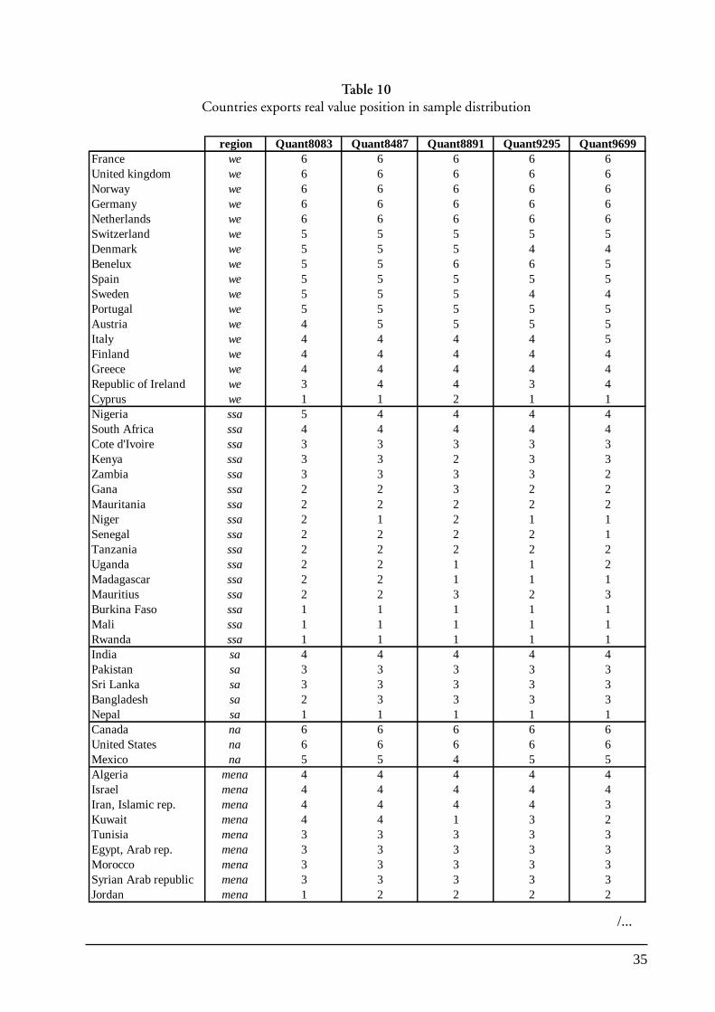
35

region Quant8083 Quant8487 Quant8891 Quant9295 Quant9699France we 6 6 6 6 6United kingdom we 6 6 6 6 6Norway we 6 6 6 6 6Germany we 6 6 6 6 6Netherlands we 6 6 6 6 6Switzerland we 5 5 5 5 5Denmark we 5 5 5 4 4Benelux we 5 5 6 6 5Spain we 5 5 5 5 5Sweden we 5 5 5 4 4Portugal we 5 5 5 5 5Austria we 4 5 5 5 5Italy we 4 4 4 4 5Finland we 4 4 4 4 4Greece we 4 4 4 4 4Republic of Ireland we 3 4 4 3 4Cyprus we 1 1 2 1 1Nigeria ssa 5 4 4 4 4South Africa ssa 4 4 4 4 4Cote d'Ivoire ssa 3 3 3 3 3Kenya ssa 3 3 2 3 3Zambia ssa 3 3 3 3 2Gana ssa 2 2 3 2 2Mauritania ssa 2 2 2 2 2Niger ssa 2 1 2 1 1Senegal ssa 2 2 2 2 1Tanzania ssa 2 2 2 2 2Uganda ssa 2 2 1 1 2Madagascar ssa 2 2 1 1 1Mauritius ssa 2 2 3 2 3Burkina Faso ssa 1 1 1 1 1Mali ssa 1 1 1 1 1Rwanda ssa 1 1 1 1 1India sa 4 4 4 4 4Pakistan sa 3 3 3 3 3Sri Lanka sa 3 3 3 3 3Bangladesh sa 2 3 3 3 3Nepal sa 1 1 1 1 1Canada na 6 6 6 6 6United States na 6 6 6 6 6Mexico na 5 5 4 5 5Algeria mena 4 4 4 4 4Israel mena 4 4 4 4 4Iran, Islamic rep. mena 4 4 4 4 3Kuwait mena 4 4 1 3 2Tunisia mena 3 3 3 3 3Egypt, Arab rep. mena 3 3 3 3 3Morocco mena 3 3 3 3 3Syrian Arab republic mena 3 3 3 3 3Jordan mena 1 2 2 2 2

/...

Table 10Countries exports real value position in sample distribution

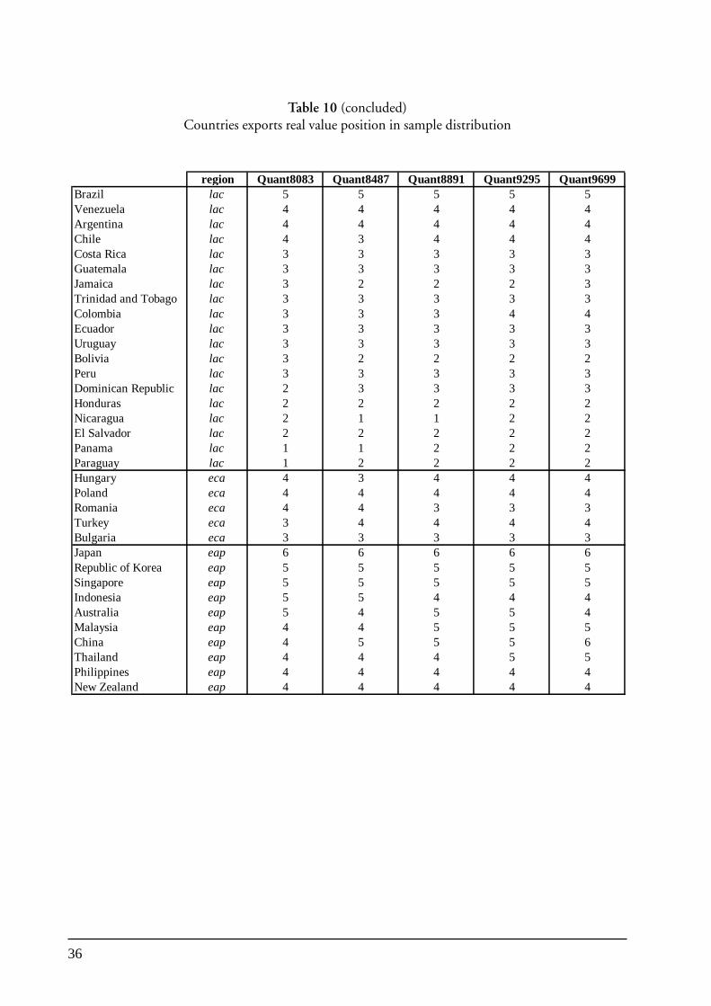
36

region Quant8083 Quant8487 Quant8891 Quant9295 Quant9699Brazil lac 5 5 5 5 5Venezuela lac 4 4 4 4 4Argentina lac 4 4 4 4 4Chile lac 4 3 4 4 4Costa Rica lac 3 3 3 3 3Guatemala lac 3 3 3 3 3Jamaica lac 3 2 2 2 3Trinidad and Tobago lac 3 3 3 3 3Colombia lac 3 3 3 4 4Ecuador lac 3 3 3 3 3Uruguay lac 3 3 3 3 3Bolivia lac 3 2 2 2 2Peru lac 3 3 3 3 3Dominican Republic lac 2 3 3 3 3Honduras lac 2 2 2 2 2Nicaragua lac 2 1 1 2 2El Salvador lac 2 2 2 2 2Panama lac 1 1 2 2 2Paraguay lac 1 2 2 2 2Hungary eca 4 3 4 4 4Poland eca 4 4 4 4 4Romania eca 4 4 3 3 3Turkey eca 3 4 4 4 4Bulgaria eca 3 3 3 3 3Japan eap 6 6 6 6 6Republic of Korea eap 5 5 5 5 5Singapore eap 5 5 5 5 5Indonesia eap 5 5 4 4 4Australia eap 5 4 5 5 4Malaysia eap 4 4 5 5 5China eap 4 5 5 5 6Thailand eap 4 4 4 5 5Philippines eap 4 4 4 4 4New Zealand eap 4 4 4 4 4

Table 10 (concluded)Countries exports real value position in sample distribution

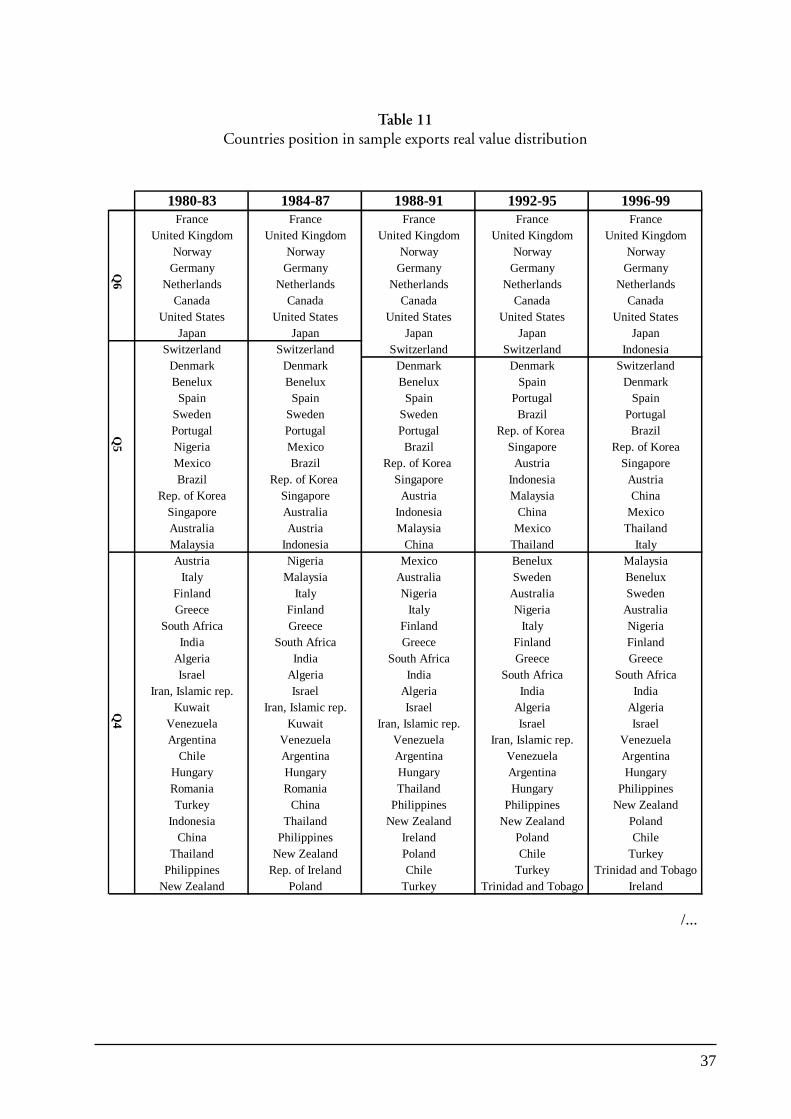
37

1980-83 1984-87 1988-91 1992-95 1996-99France France France France France

United Kingdom United Kingdom United Kingdom United Kingdom United KingdomNorway Norway Norway Norway Norway

Germany Germany Germany Germany GermanyNetherlands Netherlands Netherlands Netherlands Netherlands

Canada Canada Canada Canada CanadaUnited States United States United States United States United States

Japan Japan Japan Japan JapanSwitzerland Switzerland Switzerland Switzerland Indonesia

Denmark Denmark Denmark Denmark SwitzerlandBenelux Benelux Benelux Spain Denmark

Spain Spain Spain Portugal SpainSweden Sweden Sweden Brazil PortugalPortugal Portugal Portugal Rep. of Korea BrazilNigeria Mexico Brazil Singapore Rep. of KoreaMexico Brazil Rep. of Korea Austria SingaporeBrazil Rep. of Korea Singapore Indonesia Austria

Rep. of Korea Singapore Austria Malaysia ChinaSingapore Australia Indonesia China MexicoAustralia Austria Malaysia Mexico ThailandMalaysia Indonesia China Thailand ItalyAustria Nigeria Mexico Benelux Malaysia

Italy Malaysia Australia Sweden BeneluxFinland Italy Nigeria Australia SwedenGreece Finland Italy Nigeria Australia

South Africa Greece Finland Italy NigeriaIndia South Africa Greece Finland Finland

Algeria India South Africa Greece GreeceIsrael Algeria India South Africa South Africa

Iran, Islamic rep. Israel Algeria India IndiaKuwait Iran, Islamic rep. Israel Algeria Algeria

Venezuela Kuwait Iran, Islamic rep. Israel IsraelArgentina Venezuela Venezuela Iran, Islamic rep. Venezuela

Chile Argentina Argentina Venezuela ArgentinaHungary Hungary Hungary Argentina HungaryRomania Romania Thailand Hungary PhilippinesTurkey China Philippines Philippines New Zealand

Indonesia Thailand New Zealand New Zealand PolandChina Philippines Ireland Poland Chile

Thailand New Zealand Poland Chile TurkeyPhilippines Rep. of Ireland Chile Turkey Trinidad and Tobago

New Zealand Poland Turkey Trinidad and Tobago Ireland

Q6

Q5

Q4

Table 11Countries position in sample exports real value distribution

/...

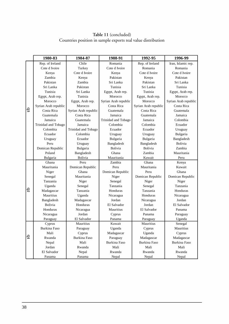
38

1980-83 1984-87 1988-91 1992-95 1996-99Rep. of Ireland Chile Romania Rep. of Ireland Iran, Islamic rep.Cote d Ivoire Turkey Cote d Ivoire Romania Romania

Kenya Cote d Ivoire Kenya Cote d Ivoire Cote d IvoireZambia Kenya Pakistan Kenya PakistanPakistan Zambia Sri Lanka Pakistan Sri LankaSri Lanka Pakistan Tunisia Sri Lanka TunisiaTunisia Sri Lanka Egypt, Arab rep. Tunisia Egypt, Arab rep.

Egypt, Arab rep. Tunisia Morocco Egypt, Arab rep. MoroccoMorocco Egypt, Arab rep. Syrian Arab republic Morocco Syrian Arab republic

Syrian Arab republic Morocco Costa Rica Syrian Arab republic Costa RicaCosta Rica Syrian Arab republic Guatemala Costa Rica GuatemalaGuatemala Costa Rica Jamaica Guatemala Jamaica

Jamaica Guatemala Trinidad and Tobago Jamaica ColombiaTrinidad and Tobago Jamaica Colombia Colombia Ecuador

Colombia Trinidad and Tobago Ecuador Ecuador UruguayEcuador Colombia Uruguay Uruguay BulgariaUruguay Ecuador Bulgaria Bulgaria Bangladesh

Peru Uruguay Bangladesh Bangladesh BoliviaDomican Republic Bulgaria Bolivia Bolivia Zambia

Poland Bangladesh Ghana Zambia MauritaniaBulgaria Bolivia Mauritania Kuwait PeruGhana Peru Zambia Ghana Kenya

Mauritania Domican Republic Peru Mauritania KuwaitNiger Ghana Domican Republic Peru Ghana

Senegal Mauritania Niger Domican Republic Domican RepublicTanzania Niger Senegal Niger NigerUganda Senegal Tanzania Senegal Tanzania

Madagascar Tanzania Honduras Tanzania HondurasMauritius Uganda Nicaragua Honduras Nicaragua

Bangladesh Madagascar Jordan Nicaragua JordanBolivia Honduras El Salvador Jordan El Salvador

Honduras Nicaragua Mauritius El Salvador PanamaNicaragua Jordan Cyprus Panama ParaguayParaguay El Salvador Panama Paraguay UgandaCyprus Mauritius Kuwait Mauritius Senegal

Burkina Faso Paraguay Uganda Cyprus MauritiusMali Cyprus Madagascar Uganda Cyprus

Rwanda Burkina Faso Paraguay Madagascar MadagascarNepal Mali Burkina Faso Burkina Faso Burkina FasoJordan Rwanda Mali Mali Mali

El Salvador Nepal Rwanda Rwanda RwandaPanama Panama Nepal Nepal Nepal

Q2

Q1

Q3

Table 11 (concluded)Countries position in sample exports real value distribution

39

However, institutions seem to matter more at a higher level of export performance. Thisresult suggests that what appears to be essential in the overall growth process as suggested byrecent research14 is only partially true for export performance. It might also suggest that institutionsand macroeconomic variables are substitutable along the export development process. While thereal exchange rate is an essential price competitiveness component for low-performers, oncemacroeconomic stability has been achieved and the composition of exports is more oriented towardscapital -intensive goods, as is most likely the case for high-performers, the institutional frameworkcomes in as an essential competitiveness ingredient. Better institutions are expected to guaranteebetter protection of property rights, which becomes essential as production becomes more andmore capital intensive. Better institutions are also likely to be associated with more efficientadministration and in particular regulation, which could prove to be important price componentsin industrialized countries.

(vii) Foreign Market Access

Results suggest that foreign market access remains essential even after controlling for supplycapacity. They do not show a time recurrent pattern. However, coefficients on foreign marketaccess reveal that it is always a significant explanatory component for under performers in allperiods as it was the case for most of the supply capacity elements analyzed above. The 1988-91period is characterized by a non-monotonic influence of FMA across quantiles. The coefficientfirst increases then falls in the Q75 regression to increase for the last quantile. The coefficient issignificant at the 1 per cent level for all quantiles. For the 1992-95 period the impact and thesignificance of the estimates decrease over the first three quantiles. Coefficients become insignificantin the upper two quantiles regressions. As export performance improves, it becomes less and lessresponsive to foreign market access. In the 1996-99 period the tendency appears to be reversed.The level of the reactivity of exports to foreign market access increases with export performance.Coefficients remain significant at the 1 per cent level for all quantiles. In some regressions increasingreturns to scale appear. The coefficient on the FMA (log) variable becomes larger than one in theQ90 quantile. From a theoretical point of view this would correspond to a small elasticity of pricesin the export sector with respect to the quantity of resources used in the sector. In other words, atsome points of the external sector performance there may be some increasing returns in the domesticsupply response to better foreign market access.15

Foreign market access is explained by various elements that include essentially geography,trade policy and partners’ characteristics, such as the size of their market and transport facilities. Itcould be the case that a more integrated world implies a more uniform set of partners’ characteristicsacross countries. As a consequence, changes in the magnitude of the estimated coefficients couldbe associated with changes in policy. However, this would be the case only if one could control forthe nature and composition of trade. In this empirical context, partner characteristics can not befully separated from policy components, so that a possible interpretation of the increased significanceof foreign market access in the upper part of the distribution across periods can be based on theevolution of the external sector structure. An associated result of that just presented is the decreasein the magnitude of the coefficient on the FDI variable across periods. The two observations puttogether suggest that linkages to international markets have become more important than thestructural development of the external sector assumed to be captured by FDI contribution to

14 See Rodrik et al. (2002) for empirical assessment and for a critical review of empirical work.15 This is a form of the home market effect as presented in Krugman (1980).

40

capital formation. This could be due to the fact that the external sector in high performing countrieshas completed its structural change, that is, its intra-sectoral development and diversification.This is plausible only if the FDI variable does proxy such a process in the upper part of thedistribution. In that context, access to international markets becomes relatively more significant indetermining export performance. This interpretation supports the argument that better access tointernational markets can contribute towards the expansion of the external sector at all stages of itsstructural development.

(e) Sensitivity Analysis

Only the most relevant results from a statistical point of view have been presented. However,a large set of variables and their combinations have been considered in estimations.

Various variables related to internal transport costs were introduced. To account for transportcosts related to internal geography the study used in turn the equivalent of the average distance

between two points in a circular country given by ( ) 5.0/33.0 πarea and, the percentage of populationliving within 100 km of the coast and rivers in 1996. The former variable is never significant. Thelatter appears to be significant and positive at high quantiles for the 1992-95 and 1996-99 periods.A larger proportion of people living close to rivers imply lower transport costs. Nevertheless, themeasure seems not to be fully appropriate for the 1989-91 period regressions. Moreover, it couldplace too much weight on water transport, which is likely to be questionable in a number ofcountries in the sample. The extent of the internal road network simply given by the total numberof kilometres of roads whether paved or not, was also used. Essentially this is due to physicalstructural transport costs. Likewise,the number of telephone lines per ‘000 people and the numberof telephone lines per employee was also considered. None of these variables turn out to besignificant, even though the coefficients appear to be correctly signed. The study also consideredvarious combinations of measures of geography-related and physical-infrastructure-related transportcosts. However, none appear to be relevant and, collinearity may be present as there are very highcross-correlation rates.

The study controlled for the macroeconomic environment using a large set of variables.First it introduced the real interest rate, which appeared to be significant for high quantiles in thelast two periods. Nevertheless, the data were available only for 74 countries, which might mitigatethe robustness of the results. The spread between the borrowing and lending rates was alsoconsidered. This variable could be seen as an indicator of the functioning of the capital market. Itremained insignificant in all regressions and was only available for 73 countries. The real effectiveexchange rate computed by the IMF was also considered. However, this was only available for afew countries, and the coefficients never appeared to be significant. The same is true for the indexof overvaluation of the currency computed by the World Bank following Dollar (1992).

Export concentration and diversification indices of exported products constructed by theUNCTAD are introduced to account for the structure of the export sector. None of these indicesappears to be significant.

All these variables were considered in various sets of explanatory variables. None generatedany result that contained a message strikingly different from those presented previously, nor wereany more relevant statistically.

41

Chapter II sheds some light on the relative importance of export performance componentsincluding to which extent that export performance has been constrained by poor supply capacityconditions. The results outlined in chapter III, helped in the understanding of the importance ofcertain elements affecting supply capacity elements in the process of export development.

The East Asian countries’ experience indicates that strong export performance is likely tosupport strong economic growth. It is thus essential to identify what determines export performance.The major components of the latter are access to international markets and supply capacity. Thisstudy investigates the relative importance of these two components. It attempts to define whetherexport performance in various regions has been constrained by either of them. Supply capacityappears to have been a limiting element of export performance in African, Middle Eastern andLatin American countries. By contrast, supply capacity has been the driving force behind theexport performance of South Asia. Empirical analysis indicates that major determinants of exportperformance are also likely to vary with the level of performance itself. Poor transport infrastructuresand a weak macroeconomic environment are expected to explain poor performance (e.g. Africancountries). The structure of the external sector is also expected to matter at all levels of exportperformance. As might be expected, foreign market access is highly significant. This has been aparticularly significant factor in explaining poor export performance for a number of countrieswhose exports are badly affected by trade barriers. However, it was also found that market accessalso affected high performing countries in the last period under investigation. Nevertheless, theywere able to overcome this constraint. This result may suggest that the structure of the externalsector and foreign market access are complements at low levels of performance and tend to becomesubstitutes at higher levels. That is to say that as the external sector structure develops, access tointernational markets becomes more significant in explaining export performance.

The above analysis suggests that policy intervention should have static and dynamic effects:

• Transport infrastructures appear to be an important determinant of exports for low-performers. Since it takes a long time to recoup investment in infrastructure and theyields tend to be low, this reinforces the argument in favour of promoting publicinvestment, either national or international, and international technical cooperationin that domain.

• Macroeconomic stability is also an important determinant of export performance atthe early stages of development of the external sector.

• Inter-sectoral diversification should be promoted at the early stage of development ofthe external sector. This could be done via the promotion of foreign direct investment,as suggested by the empirical results. This could also support arguments in favour ofmore neutral sectoral policies. However, lowering policy trade barriers on intermediateinputs could also be useful as a step toward enhancing export performance. Thusthere is scope for pushing forward the liberalization of intermediate inputs more rapidlythan final goods.

IV. POLICY IMPLICATIONS

42

• In a more dynamic context, diversification should also be promoted within sectors.This could operate through the promotion of technological improvement.Technological improvement cannot be efficiently obtained without the presence ofadequate human capital. This implies that public investment should also be devotedto raising the level of human capital (e.g. through education) and the “technologicalcompetency” of the labour force (e.g. through training). However,technologicalimprovement remains the output of technological innovation which could either beimported via FDI or nationally generated via R&D. Then, in the process of the externalsector development, inter-sectoral diversification should be associated with theaccumulation of competencies that will be able to lead to intra-sectoral diversification,which appears at latter stages of development.

• Foreign market access proves to be significant at all levels of export performance.This indicates that there is scope for further lowering trade barriers at all stages ofdevelopment of the external sector. Beside facilitating access to international marketsit would also facilitate trade in intermediate outputs. Moreover, increasing returns interms of export performance could be obtained.

• Finally, the empirical results suggest that it is necessary for policy makers to careabout all dimensions of the process of development of the external sector. For instance,fighting for better access to international markets while neglecting supply conditionsis likely to be unproductive in terms of export performance, as suggested by the Africanand to some extent the Latin American experiences.

43

While the study gives some useful guidance to policy makers, a number of points could beclarified by further work, and this would help to give greater specificity to policy guidelines.

The analysis has been carried out at an aggregate level, and in future work it may be usefulto carry forward the analysis to account for sectoral specificity.16 This should allow betterqualification of supply capacity constraints and the identification of those sectors that face themthe most severely. Analysis at the country level could then be run sector by sector as foreign marketaccess series would be obtained for each of them. This could further refine the framework forpolicy-oriented exercises.

It might also be useful to carry forward the analysis using a structural approach indetermining export performance components. This approach would allow the decomposition offoreign market access and supply capacity into well-identified elements. For instance, it wouldbecome possible to quantify the stringency of trade barriers and their impact on foreign marketaccess. Likewise, it might also be able to better assess the impact of special trade agreements andin particular of RTAs. This could be done by simply considering trade agreements partners groupingon top of, or instead of geographical grouping. It could then be assessed how much such agreementscontributed to a particular country’s or region’s export performance evolution. Typically, a pre-agreement period of time and a comparison of the underlying results with those obtained in apost-agreement period of time, could be considered. Hence, the impact on supply capacity couldbe interpreted as some sort of adjustment cost or, could serve to identify those elements thatpossibly contain the latter.

The analysis in this study did not explicitly take account of time. It is possible to compareresults across time as long as data are available. However, it should also be possible to integratetime into the cross-sectional analysis itself without making it a panel analysis. This approach wasfollowed by Dollar and Kraay (2002) who considered decadal changes in their dependent andindependent variables, that is the relationship between changes over time. The relevance of suchan approach is supported by the empirical fact that trade to GDP ratios are not strongly correlatedwith themselves across decades. This could lead to a better understanding of the decompositioncomponents influence. Practically, the total exports real value would be put as the dependentvariables, its lag T years ago (T=10 for instance), and the averages over the T years period beforethe current date of a set of control variables.

V. POSSIBLE FURTHER RESEARCH

16 Data availability in COMTRADE permits the consideration of exports at various sectorial levels rather thansimply at the aggregate level. Elbadawi, Mengistae and Zeufack (2001) adopt a similar approach using even moredisaggregated data. The data used are from more than 1400 manufacturers of textile and garments in six Sub-SaharaAfrican countries, Morocco and India. They conclude that geography is as probably as important for Africanmanufacturers as are trade policy and institutional infrastructure.

44

Alcalà F. and A. Ciccone, 2002, “Trade and Productivity”, CEPR Discussion Paper #3095.

Buchinski M., 1998, “Recent Advances in Quantile Regression Models: A Practical Guideline forEmpirical Research”, Journal of Human Resources, 33:1, pp. 88-126.

Dollar D., 1992, “Outward-Oriented Developing Countries Really Do Grow More Rapidly:Evidence from 95 LDCs, 1976-85”, Economic Development and Cultural Change, April,pp. 523-544.

Dollar D. and A. Kraay, 2002, “Institutions Trade and Growth”, forthcoming Canergie-RochesterConference Series on Public Policy.

Easterly W. and R. Levine, 2002, “Tropics, Germs, and Crops: How Endowments InfluenceEconomic Development”, NBER Working paper No. 9106.

Elbadawi I., T. Mengistae, and A. Zeufack, 2001, “Geography, Supplier Access, Foreign MarketPotential, and Manufacturing Exports in Developing countries: An Analysis of Firm LevelData”, The World Bank, Unpublished Manuscript.

Forteza and Rama, 2001, “Labor Market “Rigidity” and the Success of Economic Reforms Acrossmore the One Hundred Countries”, The World Bank Working Paper #2521.

Frankel J. A. and D. Romer, 1999, “Does Trade Cause Growth? ”, American Economic Review,89, 3, pp. 379-399.

Gallup J., J. Sachs, and A. Mellinger, 1998, “Geography and Economic Development”, Proceedingsof World bank Annual Conference on Development Economics, The World Bank:Washington.

Hall R., and C. Jones, 1998, “Fundamental Determinants of Output per Workers across Countries”,Quarterly Journal of Economics,114:1, pp.83-116.

Harrison A., 1996, “Openness and Growth: A Time-Series, Cross-Country Analysis for DevelopingCountries”, Journal of Development Economics, 48, pp. 419-77.

Irwin D.A., and M. Tervio, 2002, “Does Trade Raise Income? Evidence from the TwentiethCentury”, Journal of International Economics, 58, pp. 1-18.

Koenker R. W. and, G. Bassett, 1978, “egression Quantiles”, Econometrica, 46:1, pp. 33-50.

Krugman, P., 1980, “Scale Economies, Product Differentiation and the Pattern of Trade ”, AmericanEconomic Review, 70, pp. 950-959.

REFERENCES

45

Krugman, P. and A. Venables, 1995, “Globalization and the Inequality of Nations”, QuarterlyJournal of Economics,110:4, pp. 857-880

Limão N. and T. Venables, 2001, “Infrastrucutre, Geographical Disadvantage, Transport Costs,and Trade”, The World Bank Economic Review, 15:3, pp. 451-479.

Maksus, K. E., 2003, Comment on Redding and Venables (2003), in Challenges to Globalization:Analyzing the Economics, R. E. Baldwin and A. L Winters, eds., The University of ChicagoPress.

Redding S. and A. Venables, 2004a, “Geography and Export Performance: External Market Accessand Internal Supply Capacity”, Chapter 3, in (eds) Baldwin, R and Winters, A, Challenges toGlobalization: Analyzing the Economics, CEPR-NBER conference volume, NBER and Chi-cago University Press.

Redding S. and A. Venables, 2004b, “Economic Geography and International Inequality” (joint withAnthony Venables), Journal of International Economics, 62(1), pp. 53-82.

Rodriguez F. and D. Rodrik, 2000, ” Trade Policy and Economic Growth: A Skeptic’s Guide toCross-Sectional Evidence”, Macroeconomics Annual 2000, B. Bernanke and K. Rogoff, eds.,MIT Press for NBER.

Rodrik D., A. Subramanian and F. Trebbi, 2002, “Institutions Rule: the Primacy of Institutionsover Geography and Integration in Economic Development”, NBER Working Paper No.9305.

Sachs J. and A. M. Warner, 1995, “Economic Convergence and Economic Policies”, NBER WorkingPaper No. 5039.

UNCTAD, 1995, World Investment Report, United Nations, Geneva.

UNCTAD, 2002a, Handbook of Statistics, United Nations, Geneva.

UNCTAD, 2002b, World Investment Report, United Nations, Geneva.

UNCTAD, 2002c, Trade and Development Report, United Nations, Geneva.

The World Bank, (1993), “The East Asian Miracle: Economic Growth and Public Policy”, OxfordUniversity Press for The World Bank, New York.

Yanikkaya H., 2003, “Trade Openness and Economic Growth: A Cross-Copuntry EmpiricalInvestigation”, Journal of Development Economics, 72, pp. 57-89.

46

A. Data Sources

Bilateral Trade Flows: United Nations COMTRADE database

GDP, Population, Geographical variables (data on bilateral distance, existence of a common border):World Bank World Development Indicators

United States GDP deflator: IFS from the IMF.

Internal Geography: Gallup, Sachs and Mellinger (1998) / (www2.cid.harvard.edu/ciddata)

Miscellaneous: CIA World Fact Book

Infrastructures: World Bank WDI 2003

Trade Openness: Sachs and Warner (1995) / (www2.cid.harvard.edu/ciddata)

Labor Market Indicators: Forteza and Rama (2001)

Effective real Exchange rate Overvaluation Index: World Bank World Development Indicators (Dollar(1992) methodology)

Exchange and Interest rates: World Bank WDI 2003

FDI contribution to capital formation: UNCTAD handbook of statistics

Institutions: Expropriation risk form International Country Risk Guide database / Hall and Jones(1998) / www.standford.edu/~chadj/datasets.html

B. Geographical Country Groups

Western Europe: Austria, Belgium-Luxembourg, Switzerland, Cyprus, Germany, Denmark, Spain,Finland, France, United Kingdom, Republic of Ireland, Italy, Netherlands, Norway, Sweden, Greece,Portugal

Sub-Sahara: Burkina-Faso, Cote d’Ivoire, Ghana, Kenya, Madagascar, Mali, Mauritania, Mauritius,Niger, Nigeria, Rwanda, Senegal, Tanzania, Uganda, South Africa, Zambia, Zimbabwe

South Asia: Bangladesh, India, Sri Lanka, Nepal, Pakistan

APPENDIX

47

Middle East and North Africa: Algeria, Arab Republic of Egypt, Islamic Republic of Iran, Israel, Jordan,Kuwait, Morocco, Syrian Arab Republic, Tunisia

Latin America and Caribbean: Argentina, Bolivia, Brazil, Chile, Colombia, Costa Rica, DomicanRepublic, Ecuador, Guatemala, Honduras, Jamaica, Nicaragua, Panama, Peru, Paraguay, el Salvador,Trinidad and Tobago, Uruguay, Venezuela

Eastern Europe and Central Asia: Bulgaria, Hungary, Poland, Romania, Turkey

East Asia and the Pacific: Australia, China, Hong Kong China, Indonesia, Japan, Republic of Korea,Malaysia, New Zealand, Philippines, Singapore, Thailand, Taiwan (Province of China)

C. Quantile Regression

Quantile regression, developed by Koenker and Bassett (1978), is an extension of the classical leastsquares estimation of the conditional mean to estimation of different conditional quantile functions.The conditional mean function is estimated by minimizing the symmetrically weighted sum of absoluteerrors, where the weight is equal to 0.5. Other quantile functions are estimated by minimizing anasymmetrically weighted sum of absolute errors, where the weights are functions of the quantile ofinterest. As a consequence, quantile regression is robust to the presence of outliers.The general quantile regression model is

iii uxy θθβ += '

or alternatively

( )∫∞−

=θβ

θ'

|ix

iy dsxsf

where θβ is an unknown k x 1 vector of regression parameters associated with the θtth percentile, xi is ak x 1 vector of independent variables, yi is the dependent variable of interest and uθι is an unknown error

term. The θtth conditional quantile of y given x is ( ) θθθ β'| iii xxuQuant = . Its estimate is given by θβ̂'ix .

As θ increases continuously, the conditional distribution of y given x is traced out. Although many ofthe empirical quantile regression papers assume that the errors are independently and identicallydistributed, the only necessary assumption concerning errors is

( ) 0| =ii xuQuant θθ

48

that is, the conditional θtth quantile of the error term is equal to zero. Thus the quantile regressionapproach allows the marginal effects to change for countires at different points in the conditional

distribution by estimating θβ using several values of θ, ( )1,0∈θ . It is in this way that quantile regression

allows for parameter heterogeneity across different levels of export performance.

The quantile regression estimator is the solution to the following minimization problem:

( )

−−+−= ∑∑

<> βββθ βθβθβ

'' :

'

:

' 1minargˆ

iiii xyiii

xyiii xyxy

49

UNCTAD Study Series on

POLICY ISSUES IN INTERNATIONAL TRADEAND COMMODITIES

No. 1 Erich Supper, Is there effectively a level playing field for developing countryexports?, 2001, 138 p. Sales No. E.00.II.D.22.

No. 2 Arvind Panagariya, E-commerce, WTO and developing countries, 2000, 24 p.Sales No. E.00.II.D.23.

No. 3 Joseph Francois, Assessing the results of general equilibrium studies of multi-lateral trade negotiations, 2000, 26 p. Sales No. E.00.II.D.24.

No. 4 John Whalley, What can the developing countries infer from the UruguayRound models for future negotiations?, 2000, 29 p. Sales No. E.00.II.D.25.

No. 5 Susan Teltscher, Tariffs, taxes and electronic commerce: Revenue implicationsfor developing countries, 2000, 57 p. Sales No. E.00.II.D.36.

No. 6 Bijit Bora, Peter J. Lloyd, Mari Pangestu, Industrial policy and the WTO, 2000,47 p. Sales No. E.00.II.D.26.

No. 7 Emilio J. Medina-Smith, Is the export-led growth hypothesis valid for develop-ing countries? A case study of Costa Rica, 2001, 49 p. Sales No. E.01.II.D.8.

No. 8 Christopher Findlay, Service sector reform and development strategies: Issuesand research priorities, 2001, 24 p. Sales No. E.01.II.D.7.

No. 9 Inge Nora Neufeld, Anti-dumping and countervailing procedures – Use orabuse? Implications for developing countries, 2001, 33 p. Sales No. E.01.II.D.6.

No. 10 Robert Scollay, Regional trade agreements and developing countries: The caseof the Pacific Islands’ proposed free trade agreement, 2001, 45 p. Sales No.E.01.II.D.16.

No. 11 Robert Scollay and John Gilbert, An integrated approach to agricultural tradeand development issues: Exploring the welfare and distribution issues, 2001,43 p. Sales No. E.01.II.D.15.

No. 12 Marc Bacchetta and Bijit Bora, Post-Uruguay round market access barriersfor industrial products, 2001, 50 p. Sales No. E.01.II.D.23.

No. 13 Bijit Bora and Inge Nora Neufeld, Tariffs and the East Asian financial crisis,2001, 30 p. Sales No. E.01.II.D.27.

50

No. 14 Bijit Bora, Lucian Cernat, Alessandro Turrini, Duty and Quota-Free Access forLDCs: Further Evidence from CGE Modelling, 2002, 130 p. Sales No.E.01.II.D.22.

No. 15 Bijit Bora, John Gilbert, Robert Scollay, Assessing regional trading arrange-ments in the Asia-Pacific, 2001, 29 p. Sales No. E.01.II.D.21.

No. 16 Lucian Cernat, Assessing regional trade arrangements: Are South-South RTAsmore trade diverting?, 2001, 24 p. Sales No. E.01.II.D.32.

No. 17 Bijit Bora, Trade related investment measures and the WTO: 1995-2001, 2002.

No. 18 Bijit Bora, Aki Kuwahara, Sam Laird, Quantification of non-tariff measures,2002, 42 p. Sales No. E.02.II.D.8.

No. 19 Greg McGuire, Trade in services – Market access opportunities and the ben-efits of liberalization for developing economies, 2002, 45 p. Sales No. E.02.II.D.9.

No. 20 Alessandro Turrini, International trade and labour market performance: majorfindings and open questions, 2002, 30 p. Sales No. E.02.II.D.10.

No. 21 Lucian Cernat, Assessing south-south regional integration: same issues, manymetrics, 2003, 32 p. Sales No. E.02.II.D.11.

No. 22 Kym Anderson, Agriculture, trade reform and poverty reduction: implicationsfor Sub-Saharan Africa, 2004, Sales No. E.04.II.D.5.

No. 23 Ralf Peters and David Vanzetti, Shifting sands: searching for a compromise inthe WTO negotiations on agriculture, 2004, Sales No. E.04.II.D.4.

No. 24 David Vanzetti, User manual and handbook on agricultural trade policy simu-lation model (ATPSM), 2004, Sales No. E.04.II.D.3.

No. 25 Khalilur Rahman, Crawling out of snake pit: special and differential treat-ment and post-Cancun imperatives, 2004, Sales No. E.04.II.D.8.

No. 26 Marco Fugazza, Export performance and its determinants: supply and de-mand constraints, 2004, 59 p. Sales No. E.04.II.D.20.

51

United Nations publications may be obtained from bookstores and distributors throughout the world.Please consult your bookstore or write to:

United Nations Publications

All orders from North America, Latin America, the Caribbean and Asia and the Pacific shouldbe sent to:

United Nations PublicationsRoom DC2-853, 2 UN PlazaNew York, NY 10017, USATelephone: (212) 963-8302, Toll Free 1-800-253-9646 (North America only)Fax: (212) 963-3489E-mail: [email protected]

Customers in Europe, Africa and the Middle East should send their orders to:Section des Ventes et CommercialisationBureau E-4, CH-1211Geneva 10, SwitzerlandTelephone: 41 (22) 917-2613/2614Fax: 41 (22) 917-0027E-mail: [email protected]

53

QUESTIONNAIRE

UNCTAD Study Series onPOLICY ISSUES IN INTERNATIONAL TRADE

AND COMMODITIES(Study series no. 26: Export Performance and Its Determinants:

Supply and Demand Constraints)

Readership SurveySince 1999, the Trade Analysis Branch of the Division on International Trade in Goods and

Services, and Commodities of UNCTAD has been carrying out policy-oriented analytical workaimed at improving the understanding of current and emerging issues in international trade ofconcern to developing countries. In order to improve the quality of the work of the Branch, itwould be useful to receive the views of readers on this and other similar publications. It wouldtherefore be greatly appreciated if you could complete the following questionnaire and return to:

Jenifer Tacardon-MercadoTAB/DITC, Rm. E-8076

United Nations Conference on Trade and DevelopmentPalais des Nations

CH-1211 Geneva 10, Switzerland

1. Name and address of respondent (optional):

2. Which of the following describes your area of work?

Government Public enterprisePrivate enterprise institution Academic or researchInternational organization MediaNot-for-profit organization Other (specify) _________________

3. In which country do you work? _________________________________________

4. Did you find this publication Very useful Of some use Little useto your work?

5. What is your assessment of the contents of this publication? Excellent Good Adequate Poor

6. Other comments:

export performance and its determinants: supply … models_marco/export perfomance.pdf ·...

Documents