explanatory notes to senior secondary mathematics ... · pdf fileexplanatory notes to senior...
TRANSCRIPT
Explanatory Notes toSenior Secondary Mathematics Curriculum Module 1 (Calculus and Statistics)-
Mathematics Education SectionCurriculum Development Institute
Education BureauCopyright: ©HKSAR Education bureau, 2009. Content in this booklet may be used for non-profit-making educational purposes with proper acknowledgement
ISBN 978-988-8040-39-1
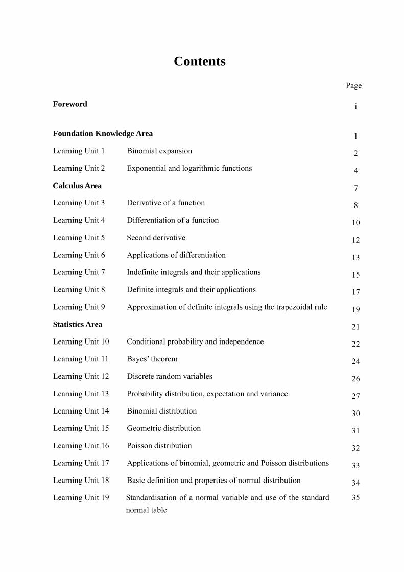
Contents
Page
Foreword i
Foundation Knowledge Area 1
Learning Unit 1 Binomial expansion 2
Learning Unit 2 Exponential and logarithmic functions 4
Calculus Area 7
Learning Unit 3 Derivative of a function 8
Learning Unit 4 Differentiation of a function 10
Learning Unit 5 Second derivative 12
Learning Unit 6 Applications of differentiation 13
Learning Unit 7 Indefinite integrals and their applications 15
Learning Unit 8 Definite integrals and their applications 17
Learning Unit 9 Approximation of definite integrals using the trapezoidal rule 19
Statistics Area 21
Learning Unit 10 Conditional probability and independence 22
Learning Unit 11 Bayes’ theorem 24
Learning Unit 12 Discrete random variables 26
Learning Unit 13 Probability distribution, expectation and variance 27
Learning Unit 14 Binomial distribution 30
Learning Unit 15 Geometric distribution 31
Learning Unit 16 Poisson distribution 32
Learning Unit 17 Applications of binomial, geometric and Poisson distributions 33
Learning Unit 18 Basic definition and properties of normal distribution 34
Learning Unit 19 Standardisation of a normal variable and use of the standard
normal table
35
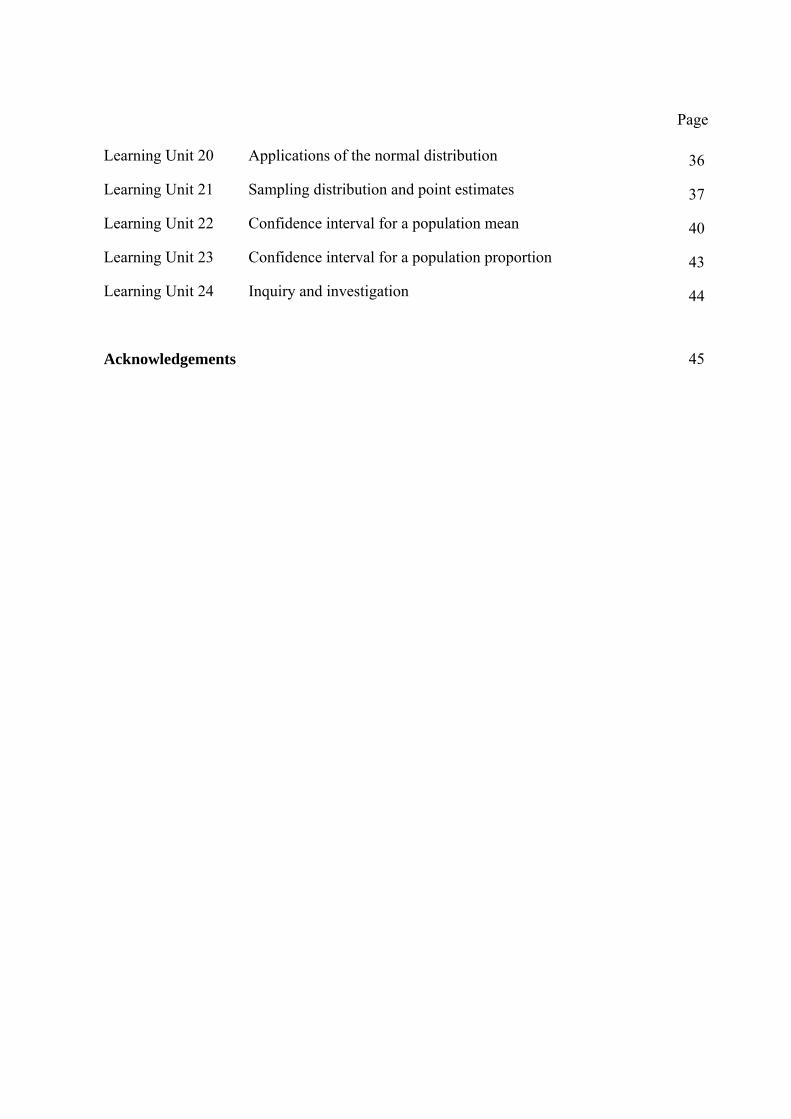
Page
Learning Unit 20 Applications of the normal distribution 36
Learning Unit 21 Sampling distribution and point estimates 37
Learning Unit 22 Confidence interval for a population mean 40
Learning Unit 23 Confidence interval for a population proportion 43
Learning Unit 24 Inquiry and investigation 44
Acknowledgements 45
i
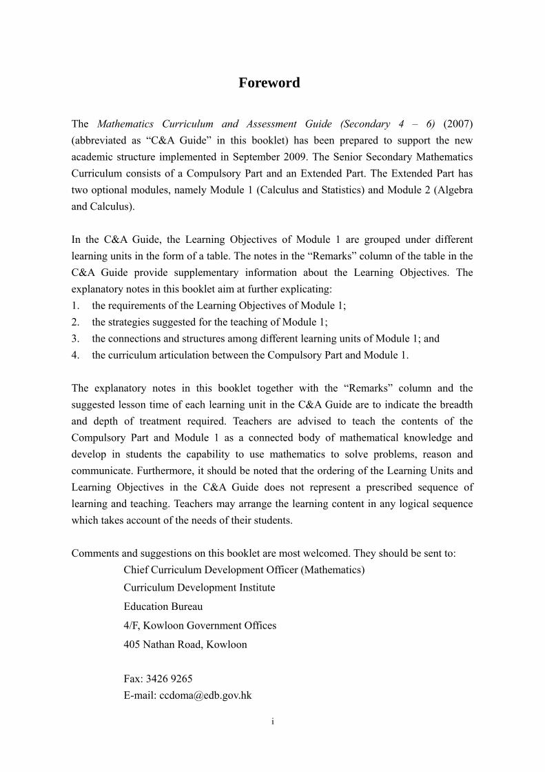
Foreword
The Mathematics Curriculum and Assessment Guide (Secondary 4 – 6) (2007)
(abbreviated as “C&A Guide” in this booklet) has been prepared to support the new
academic structure implemented in September 2009. The Senior Secondary Mathematics
Curriculum consists of a Compulsory Part and an Extended Part. The Extended Part has
two optional modules, namely Module 1 (Calculus and Statistics) and Module 2 (Algebra
and Calculus).
In the C&A Guide, the Learning Objectives of Module 1 are grouped under different
learning units in the form of a table. The notes in the “Remarks” column of the table in the
C&A Guide provide supplementary information about the Learning Objectives. The
explanatory notes in this booklet aim at further explicating:
1. the requirements of the Learning Objectives of Module 1;
2. the strategies suggested for the teaching of Module 1;
3. the connections and structures among different learning units of Module 1; and
4. the curriculum articulation between the Compulsory Part and Module 1.
The explanatory notes in this booklet together with the “Remarks” column and the
suggested lesson time of each learning unit in the C&A Guide are to indicate the breadth
and depth of treatment required. Teachers are advised to teach the contents of the
Compulsory Part and Module 1 as a connected body of mathematical knowledge and
develop in students the capability to use mathematics to solve problems, reason and
communicate. Furthermore, it should be noted that the ordering of the Learning Units and
Learning Objectives in the C&A Guide does not represent a prescribed sequence of
learning and teaching. Teachers may arrange the learning content in any logical sequence
which takes account of the needs of their students.
Comments and suggestions on this booklet are most welcomed. They should be sent to:
Chief Curriculum Development Officer (Mathematics)
Curriculum Development Institute
Education Bureau
4/F, Kowloon Government Offices
405 Nathan Road, Kowloon
Fax: 3426 9265
E-mail: [email protected]

ii
(Blank Page)
1
Foundation Knowledge Area
The content of Foundation Knowledge Area consists of two Learning Units. The first
Learning Unit “Binomial Expansion” forms the basis of the binomial distribution.
The second Learning Unit is “Exponential and Logarithmic functions”. Many
mathematical models related to natural phenomena involve the exponential function.
The probability function of the normal distribution also involves the exponential
function.
It should be noted that the content of Foundation Knowledge Area is considered as
pre-requisite knowledge for Calculus Area and Statistics Area of Module 1. Rigorous
treatment of the topics in Foundation Knowledge should be avoided.
2
Learning Unit Learning Objective Time
Foundation Knowledge Area
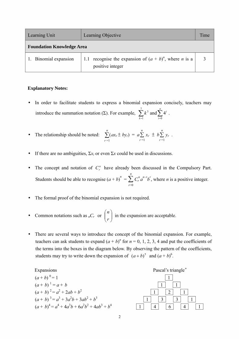
1. Binomial expansion 1.1 recognise the expansion of (a + b)n, where n is a
positive integer
3
Explanatory Notes:
In order to facilitate students to express a binomial expansion concisely, teachers may
introduce the summation notation (Σ). For example,
7
1
3
k
k and
n
i
i
0
4 .
The relationship should be noted: r =1
n
( axr ± byr) = ar =1
n
xr ± br =1
n
yr .
If there are no ambiguities, Σxi or even Σx could be used in discussions.
The concept and notation of nrC have already been discussed in the Compulsory Part.
Students should be able to recognise (a + b)n
= r=0
n
C nr a
n–rb
r, where n is a positive integer.
The formal proof of the binomial expansion is not required.
Common notations such as nCr or
r
n in the expansion are acceptable.
There are several ways to introduce the concept of the binomial expansion. For example,
teachers can ask students to expand (a + b)n for n = 0, 1, 2, 3, 4 and put the coefficients of
the terms into the boxes in the diagram below. By observing the pattern of the coefficients,
students may try to write down the expansion of 5)( ba and (a + b)6.
Expansions Pascal’s triangle*
(a + b) 0 = 1 1
(a + b) 1 = a + b 1 1
(a + b) 2 = a2 + 2ab + b2 1 2 1
(a + b) 3 = a3 + 3a2b + 3ab2 + b3 1 3 3 1
(a + b)4 = a4 + 4a3b + 6a2b2 + 4ab3 + b4 1 4 6 4 1
3
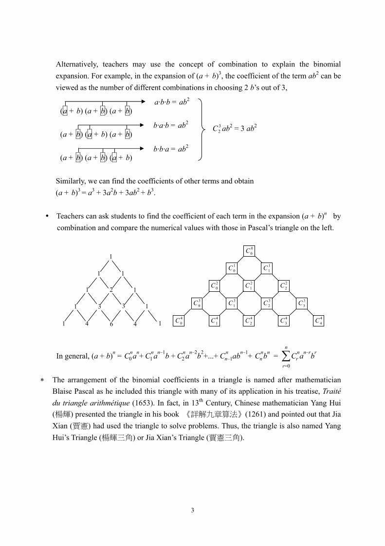
Alternatively, teachers may use the concept of combination to explain the binomial
expansion. For example, in the expansion of (a + b)3, the coefficient of the term ab2 can be
viewed as the number of different combinations in choosing 2 b’s out of 3,
(a + b) (a + b) (a + b)
(a + b) (a + b) (a + b)
(a + b) (a + b) (a + b)
Similarly, we can find the coefficients of other terms and obtain
(a + b)3 = a3 + 3a2b + 3ab2 + b3.
Teachers can ask students to find the coefficient of each term in the expansion (a + b)n by
combination and compare the numerical values with those in Pascal’s triangle on the left.
In general, (a + b)n
= C n 0 a
n+ C n 1 a
n–1b + C
n 2 an–2
b2+...+ C
n n–1abn–1
+ C n n b
n =
r=0
n
C n r a
n–rb
r
The arrangement of the binomial coefficients in a triangle is named after mathematician
Blaise Pascal as he included this triangle with many of its application in his treatise, Traité
du triangle arithmétique (1653). In fact, in 13th Century, Chinese mathematician Yang Hui
(楊輝) presented the triangle in his book 《詳解九章算法》(1261) and pointed out that Jia
Xian (賈憲) had used the triangle to solve problems. Thus, the triangle is also named Yang
Hui’s Triangle (楊輝三角) or Jia Xian’s Triangle (賈憲三角).
1
1 1
1
3 1
1
1 3
2
6 4 1 4 1
C 00
C 10
C 31C 3
0
C 2 2 C 21C 2
0
C 11
C 32 C 3 3
C 41C 4
0 C 42 C 4 3 C 4 4
32C ab2 = 3 ab2
a·b·b = ab2
b·a·b = ab2
b·b·a = ab2
4
Learning Unit Learning Objective Time
Foundation Knowledge Area
2. Exponential and
logarithmic functions
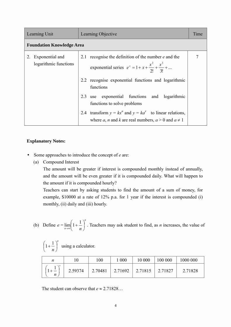
2.1 recognise the definition of the number e and the
exponential series ...!3!2
132
xx
xe x
2.2 recognise exponential functions and logarithmic
functions
2.3 use exponential functions and logarithmic
functions to solve problems
2.4 transform y = kxn and y = kax to linear relations,
where a, n and k are real numbers, a > 0 and a 1
7
Explanatory Notes:
Some approaches to introduce the concept of e are:
(a) Compound Interest
The amount will be greater if interest is compounded monthly instead of annually,
and the amount will be even greater if it is compounded daily. What will happen to
the amount if it is compounded hourly?
Teachers can start by asking students to find the amount of a sum of money, for
example, $10000 at a rate of 12% p.a. for 1 year if the interest is compounded (i)
monthly, (ii) daily and (iii) hourly.
(b) Define e =n
n n
11lim . Teachers may ask student to find, as n increases, the value of
n
n
11 using a calculator.
n 10 100 1 000 10 000 100 000 1000 000 n
n
11 2.59374 2.70481 2.71692 2.71815 2.71827 2.71828
The student can observe that e 2.71828…
5
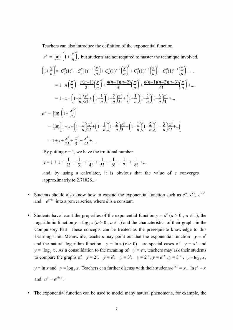
Teachers can also introduce the definition of the exponential function
ex = lim
n→∞
1+
xn
n
, but students are not required to master the technique involved.
1+
xn
n
= C n 0 (1)
n + C n 1 (1)
n-1
xn + C
n 2 (1)n-2
xn
2
+ C n 3 (1)
n-3
xn
3
+ C n 4 (1)
n-4
xn
4
+...
= 1 + n
xn +
n(n – 1)2!
xn
2
+
n(n – 1)(n – 2)3!
xn
3
+
n(n – 1)(n – 2)(n – 3)4!
xn
4
+...
= 1 + x +
1 –
1n
x 2
2! +
1 –
1n
1 –
2n
x 3
3! +
1 –
1n
1 –
2n
1 –
3n
x 4
4! +...
ex = lim
n→∞
1+
xn
n
= limn→∞
1 + x +
1 –
1n
x 2
2! +
1 –
1n
1 –
2n
x 3
3! +
1 –
1n
1 –
2n
1 –
3n
x 4
4! +...
= 1 + x +
x 2
2! +
x 3
3! +
x 4
4! +...
By putting x = 1, we have the irrational number
e = 1 + 1 + 12!
+ 13!
+ 14!
+ 15!
+ 16!
+ 17!
+ 18!
+...
and, by using a calculator, it is obvious that the value of e converges
approximately to 2.71828...
Students should also know how to expand the exponential function such as e-x, ekx, 2xe
and ex+k into a power series, where k is a constant.
Students have learnt the properties of the exponential function y = ax (a > 0 , a 1), the
logarithmic function y = log a x (a > 0 , a 1) and the characteristics of their graphs in the
Compulsory Part. These concepts can be treated as the prerequisite knowledge to this
Learning Unit. Meanwhile, teachers may point out that the exponential function y = ex
and the natural logarithm function y = ln x (x > 0) are special cases of y = a
x and y = xalog . As a consolidation to the meaning of y = e
x, teachers may ask their students
to compare the graphs of y = 2x, y = ex, y = 3x, y = 2–x , y = e
–x , y = 3–x , xy 2log ,
y = ln x and xy 3log . Teachers can further discuss with their students xe x ln , xex ln
and axx ea ln .
The exponential function can be used to model many natural phenomena, for example, the
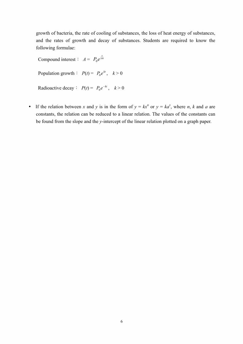
6
growth of bacteria, the rate of cooling of substances, the loss of heat energy of substances,
and the rates of growth and decay of substances. Students are required to know the
following formulae:
Compound interest: A = 1000
rt
eP
Population growth: P(t) = kteP0 , k > 0
Radioactive decay: P(t) = kteP 0 , k > 0
If the relation between x and y is in the form of y = kxn or y = kax, where n, k and a are
constants, the relation can be reduced to a linear relation. The values of the constants can
be found from the slope and the y-intercept of the linear relation plotted on a graph paper.
7
Calculus Area
Calculus Area consists of two sections, namely Differentiation with Its Applications
and Integration with Its Applications. The concept of the derivative of a function
involves the concept of the limit of a function. In the section “Differentiation and Its
Applications”, students should understand the definition of the derivative of a
function, the fundamental formulae and the rules of differentiation. They should also
be able to use derivatives to find the equation of the tangent to a curve and to
investigate the maximum/minimum values of a function.
Students need to find the function f(x) from its derivative xf in various situations
related to science, technology and economics. This reverse process is the idea of the
indefinite integral. Teachers need to explain clearly the idea of the definite integral as
the numerical limit of a summation. Teacher can lead students to recognise that the
Fundamental Theorem of Calculus can link the two apparently different concepts (the
indefinite integral and the definite integral) together.
Notations should be firmly established and well understood by students.
The approaches adopted should be intuitive but the concepts involved should be
correct. In difficult topics such as limits, numerical approaches using calculators (or
computer software) can help students understand the related concepts without paying
attention to abstract definitions. Teachers can make use of graphing tools (such as
Graphmatica, Winplot etc.) to illustrate the concepts.
8
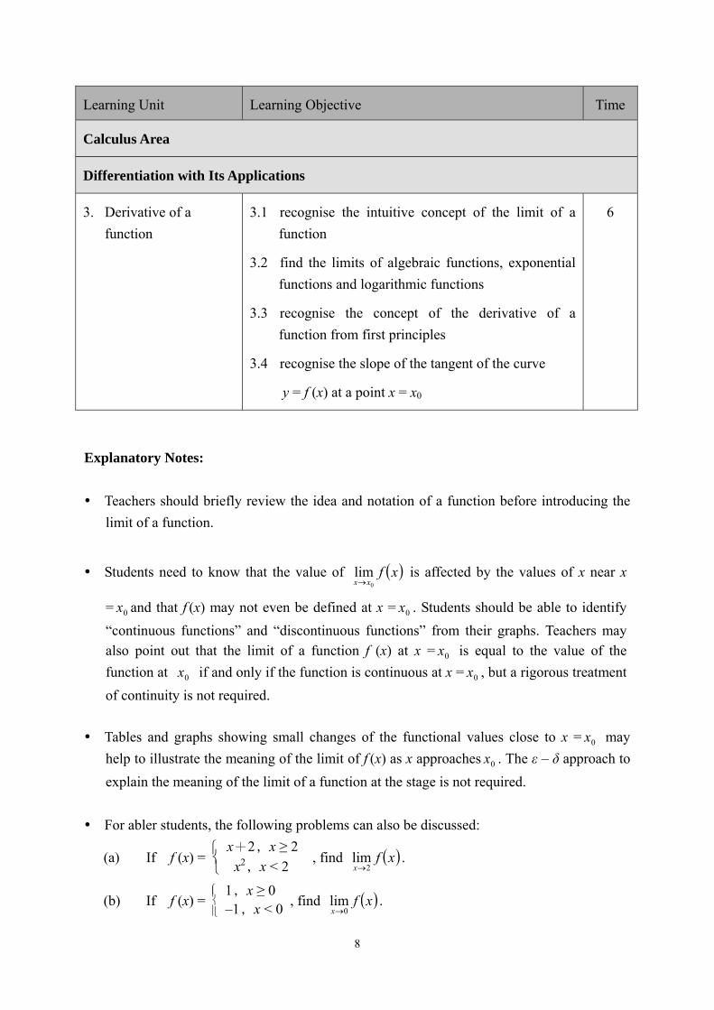
Learning Unit Learning Objective Time
Calculus Area
Differentiation with Its Applications
3. Derivative of a
function
3.1 recognise the intuitive concept of the limit of a
function
3.2 find the limits of algebraic functions, exponential
functions and logarithmic functions
3.3 recognise the concept of the derivative of a
function from first principles
3.4 recognise the slope of the tangent of the curve
y = f (x) at a point x = x0
6
Explanatory Notes:
Teachers should briefly review the idea and notation of a function before introducing the
limit of a function.
Students need to know that the value of xfxx 0
lim
is affected by the values of x near x
= 0x and that f (x) may not even be defined at x = 0x . Students should be able to identify
“continuous functions” and “discontinuous functions” from their graphs. Teachers may
also point out that the limit of a function f (x) at x = 0x is equal to the value of the
function at 0x if and only if the function is continuous at x = 0x , but a rigorous treatment
of continuity is not required.
Tables and graphs showing small changes of the functional values close to x = 0x may
help to illustrate the meaning of the limit of f (x) as x approaches 0x . The ε – δ approach to
explain the meaning of the limit of a function at the stage is not required.
For abler students, the following problems can also be discussed:
(a) If f (x) = x+2﹐x ≥ 2
x2﹐x < 2 , find xf
x 2lim
.
(b) If f (x) = 1﹐x ≥ 0–1﹐x < 0
, find xfx 0lim
.
9
Students should be able to find the limits of algebraic functions, exponential functions and
logarithmic functions by using limits of sum, difference, product, quotient and
composition. When x tends to infinity, students should know that 1x tends to zero.
Students are also required to find the limits of some simple functions such as3
32
x
x and
xxe
3 as x approaches infinity.
The derivative of a function y = f(x) with respect to x can be defined as
x
xfxxf
x
yxx
00limlim if the limit exists. Teachers may demonstrate how to find
the derivative of simple functions like x2 and 1
x-1 from first principles. However,
students are not required to find the derivatives of functions from first principles.
Teachers may introduce the geometrical meaning of the difference quotient
x
xfxxf
x
y
. Students should know common notations of derivative such as y ,
f (x) and dydx . They should understand that
ddx is an operator and
dydx should not be taken
as a fraction.
Students should recognise the notations of f ( 0x ) and 0xxdx
dy
, where x0 is a given value.
Students should understand that as x approaches 0, the limiting value of yx
will give
the slope of the tangent to the curve at the point ( 0x , f ( 0x )). They should also be able to
find the equations of tangents of simple curves.
10
Learning Unit Learning Objective Time
Calculus Area
Differentiation with Its Applications
4. Differentiation of a
function
4.1 understand the addition rule, product rule, quotient
rule and chain rule of differentiation
4.2 find the derivatives of algebraic functions,
exponential functions and logarithmic functions
10
Explanatory Notes:
Teachers may derive the rules of differentiation. Students should grasp these basic rules to
find the derivatives of functions.
Teachers may give some typical examples of composite functions and inverse functions
and then introduce the chain rule dydx =
dydu ·
dudx. Students do not need to understand the
differentiation of inverse functions, but they may use the formula dxdy =
1dydx
to solve
problems. Differentiation of parametric equations is not required.
Students should learn how to differentiate a polynomial. When rules for differentiating the
sum, the product and the quotient of functions are established, students should be able to
differentiate the product of polynomials and rational functions such as (2x + 3)(4x2 + 5)
and x
x
32
21 2
.
Students do not need to learn implicit differentiation, but they should know how to carry
out logarithmic differentiation. When it is required to differentiate functions of the form
h(x)k(x), h(x)k(x) or [h(x)]k(x), where h(x) and k(x) are functions of x, it is easier to find their
derivatives by logarithmic differentiation. For example, in finding the derivative of the
functions ),4)(3)(2)(1( xxxx 1
13
xx
x and xxy .

11
Students should know how to use Chain rule to find the derivatives of functions of the
form )(xfey and )(ln xfy .
Students should know how to find the derivatives of composite functions such as
12xe and ln 3x2-5x+7.
12
Learning Unit Learning Objective Time
Calculus Area
Differentiation with Its Applications
5. Second derivative 5.1 recognise the concept of the second derivative of a
function
5.2 find the second derivative of an explicit function
2
Explanatory Notes:
The second derivative may be obtained by differentiating the first derivative. If )(= xfy ,
the second derivative may be written as f ˝(x), y˝ or 2
2
dx
yd.
Teachers may point out that, in general,
2
22
2 1
dy
xddx
yd and
2
2
2
dx
dy
dx
yd.
13
Learning Unit Learning Objective Time
Calculus Area
Differentiation with Its Applications
6. Applications of
differentiation
6.1 use differentiation to solve problems involving
tangents, rates of change, maxima and minima
9
Explanatory Notes:
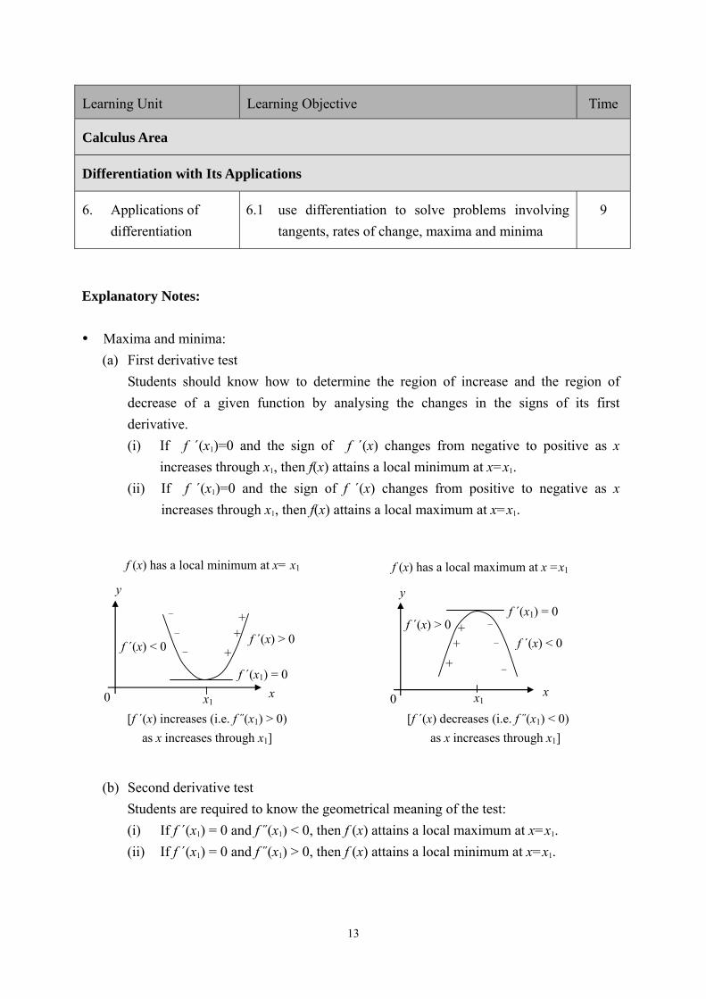
Maxima and minima:
(a) First derivative test
Students should know how to determine the region of increase and the region of
decrease of a given function by analysing the changes in the signs of its first
derivative.
(i) If f ΄(x1)=0 and the sign of f ΄(x) changes from negative to positive as x
increases through x1, then f(x) attains a local minimum at x=x1.
(ii) If f ΄(x1)=0 and the sign of f ΄(x) changes from positive to negative as x
increases through x1, then f(x) attains a local maximum at x=x1.
f (x) has a local minimum at x= x1 f (x) has a local maximum at x =x1
f ΄(x) > 0 f ΄(x) < 0
f ΄(x1) = 0
x 0
y
+
+
+
x1
–
–
–
[f ΄(x) increases (i.e. f ˝(x1) > 0)
as x increases through x1]
f ΄(x) > 0
f ΄(x) < 0
f ΄(x1) = 0
x 0
y
+
+
+
x1
–
–
–
[f ΄(x) decreases (i.e. f ˝(x1) < 0)
as x increases through x1]
(b) Second derivative test
Students are required to know the geometrical meaning of the test:
(i) If f ΄(x1) = 0 and f ˝(x1) < 0, then f (x) attains a local maximum at x=x1.
(ii) If f ΄(x1) = 0 and f ˝(x1) > 0, then f (x) attains a local minimum at x=x1.
14
The local extremum is not necessarily the global extremum. In finding the global
extremum in an optimization problem, students should also consider the values at the end
points of the interval(s) concerned.
Students should be able to apply either the first derivative test or the second derivative test
to find the extrema of a function. When f ˝(x1) = 0, the second derivative test is not
applicable to find the local extrema. In this case, students have to revert to the first
derivative test.
Students should be able to use the second derivative to determine the concavity and
convexity of a function. They are not required to sketch the graph of the function.
Students are not required to learn the concept of the point of inflexion of a curve. Local
extrema at x = x1 related to the non-existence of f ΄(x1) are not required.
15
Learning Unit Learning Objective Time
Calculus Area
Integration with Its Applications
7. Indefinite integrals
and their applications
7.1 recognise the concept of indefinite integration
7.2 understand the basic properties of indefinite
integrals and basic integration formulae
7.3 use basic integration formulae to find the
indefinite integrals of algebraic functions and
exponential functions
7.4 use integration by substitution to find indefinite
integrals
7.5 use indefinite integration to solve problems
10
Explanatory Notes:
The terms “integrand” and “constant of integration” should be introduced. Students should
note that indefinite integration is the reverse process of differentiation.
Students are required to master the following rules:
k f (x)dx = k f (x)dx , where k is a constant
[ f (x) ± g (x)]dx = f (x)dx ± g (x)dx
k dx = kx + C , where k and C are constants
xn dx = xn +1
n+1 + C , where C is a constant, n is real and n ≠ –1 (n = 0 should also
be discussed)
1x dx = ln x + C , x ≠ 0
ex dx = ex + C
In order to change the integrand into one of the forms of the basic integration formulae,

16
students need to substitute )(tx and hence f (x)dx = f [(t)](t)dt . Teachers
may introduce integration by substitution through examples, such as (2x + 1)5dx and
2x x2 + 1 dx .
Using integration by parts to find indefinite integral is not required.
17
Learning Unit Learning Objectives Time
Calculus Area
Integration with Its Applications
8. Definite integrals and
their applications
8.1 recognise the concept of definite integration
8.2 recognise the Fundamental Theorem of Calculus
and understand the properties of definite integrals
8.3 find the definite integrals of algebraic functions
and exponential functions
8.4 use integration by substitution to find definite
integrals
8.5 use definite integration to find the areas of plane
figures
8.6 use definite integration to solve problems
15
Explanatory Notes:
The definite integral can be introduced by considering the area under the curve to
distinguish its concept from that of the indefinite integral.
Some properties of the definite integral are useful. Their geometrical meaning should be
explored.
a
bf (x) dx = –
b
af (x) dx
a
af (x) dx = 0
b
af (x) dx =
c
af (x) dx +
b
cf (x) dx
b
ak f (x) dx = k
b
af (x) dx , where k is a constant
b
a[ f (x) ± g (x)]dx =
b
af (x) dx ±
b
ag (x) dx

18
Students should know that the above formulae can only be applied when the functions
under discussion are continuous in the interval [a, b].
When the method of substitution is used to evaluate a definite integral, students should be
reminded that the upper and lower limits of the definite integral should be changed
accordingly.
19
Learning Unit Learning Objective Time
Calculus Area
Integration with Its Applications
9. Approximation of
definite integrals
using the trapezoidal
rule
9.1 understand the trapezoidal rule and use it to
estimate the values of definite integrals
4
Explanatory Notes:
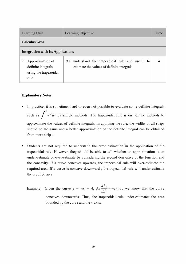
In practice, it is sometimes hard or even not possible to evaluate some definite integrals
such as 2
1e
x 22
dx by simple methods. The trapezoidal rule is one of the methods to
approximate the values of definite integrals. In applying the rule, the widths of all strips
should be the same and a better approximation of the definite integral can be obtained
from more strips.
Students are not required to understand the error estimation in the application of the
trapezoidal rule. However, they should be able to tell whether an approximation is an
under-estimate or over-estimate by considering the second derivative of the function and
the concavity. If a curve concaves upwards, the trapezoidal rule will over-estimate the
required area. If a curve is concave downwards, the trapezoidal rule will under-estimate
the required area.
Example Given the curve y = –x2 + 4. As 022
2
dx
yd, we know that the curve
concaves downwards. Thus, the trapezoidal rule under-estimates the area
bounded by the curve and the x-axis.

20
(Blank page)
21
Statistics Area
Statistics Area consists of four sections, namely Further Probability; Binomial,
Geometric and Poisson Distributions and Their Applications; Normal Distribution
and Its Applications; and Point and Interval Estimation.
Probability is considered elementary and important in this Area. The concept of a
random variable is new to students. Binomial, geometric, Poisson and normal
distributions serve to widen students’ knowledge on probability distributions.
Discussions of statistical inference are also included.
A study of population parameters and sample statistics depicts the relationship
between populations and samples. Point estimation and interval estimation are
included.
Point estimation involves the use of sample data to calculate a statistic which is to
serve as a guess for an unknown population parameter. A confidence interval (CI) is
an interval estimate of a population parameter. Confidence intervals are used to
indicate the reliability of an estimate. How likely the interval is to contain the
parameter is determined by the confidence level. When the desired confidence level is
increased, the corresponding confidence interval will be widened.

22
Learning Unit Learning Objective Time
Statistics Area
Further Probability
10. Conditional
probability and
independence
10.1 Understand the concepts of conditional
probability and independent events
10.2 use the laws P(A B) = P(A) P(B | A) and
P(D | C) = P(D) for independent events C and D
to solve problems
3
Explanatory Notes:
The addition law and multiplication law of probability, the concepts of exclusive events,
complementary events, independent events and conditional probability are discussed in
Learning Unit 15 in the Compulsory Part. Students need to further investigate conditional
probability in this Learning Unit.
Venn diagrams can be used to illustrate the meaning of conditional probabilities before the
introduction of P(B | A) = P(AB)
P(A) , where A may be considered as a reduced sample
space. It is straightforward to arrive at the law P(AB) = P(A)P(B | A).
Students may have confusions in the concepts related to P(B A) and P(A B).
Students should note the following points about mutually independent events:
If two events A and B are mutually independent, then the occurrence of A (or B) does
not affect the probability of the occurrence of B (or A).
If two events A and B are mutually independent, then A and B, B and A, A and
B are also mutually independent.
The difference between “mutually independent events” and “mutually exclusive events”
should be discussed. Two events are mutually independent if the occurrence of one event
does not affect the probability of the occurrence of another event. Two events are mutually
exclusive if they cannot happen at the same time.
23
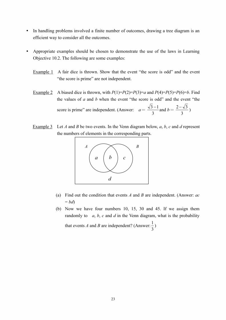
In handling problems involved a finite number of outcomes, drawing a tree diagram is an
efficient way to consider all the outcomes.
Appropriate examples should be chosen to demonstrate the use of the laws in Learning
Objective 10.2. The following are some examples:
Example 1 A fair dice is thrown. Show that the event “the score is odd” and the event
“the score is prime” are not independent.
Example 2 A biased dice is thrown, with P(1)=P(2)=P(3)=a and P(4)=P(5)=P(6)=b. Find
the values of a and b when the event “the score is odd” and the event “the
score is prime” are independent. (Answer: a=3
13 and b=
3
32)
Example 3 Let A and B be two events. In the Venn diagram below, a, b, c and d represent
the numbers of elements in the corresponding parts.
A B
a c
d
b
(a) Find out the condition that events A and B are independent. (Answer: ac
= bd)
(b) Now we have four numbers 10, 15, 30 and 45. If we assign them
randomly to a, b, c and d in the Venn diagram, what is the probability
that events A and B are independent? (Answer:3
1)
24
Learning Unit Learning Objective Time
Statistics Area
Further Probability
11. Bayes’ theorem 11.1 use Bayes’ theorem to solve simple problems 4
Explanatory Notes:
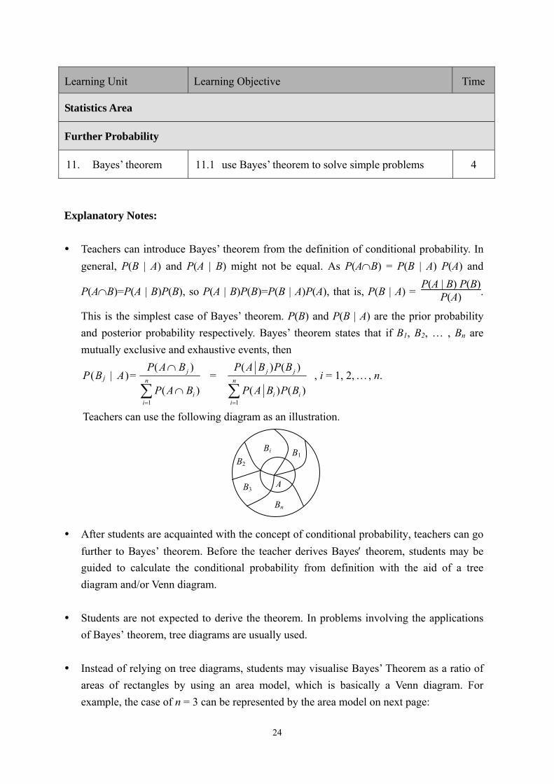
Teachers can introduce Bayes’ theorem from the definition of conditional probability. In
general, P(B | A) and P(A | B) might not be equal. As P(AB) = P(B | A) P(A) and
P(AB)=P(A | B)P(B), so P(A | B)P(B)=P(B | A)P(A), that is, P(B | A) = P(A | B) P(B)
P(A) .
This is the simplest case of Bayes’ theorem. P(B) and P(B | A) are the prior probability
and posterior probability respectively. Bayes’ theorem states that if B1, B2, … , Bn are
mutually exclusive and exhaustive events, then
P(Bj | A)=
n
ii
j
BAP
BAP
1
)(
)( =
n
iii
jj
BPBAP
BPBAP
1
)()(
)()( , i = 1, 2, , n.
Teachers can use the following diagram as an illustration.
After students are acquainted with the concept of conditional probability, teachers can go
further to Bayes’ theorem. Before the teacher derives Bayes theorem, students may be
guided to calculate the conditional probability from definition with the aid of a tree
diagram and/or Venn diagram.
Students are not expected to derive the theorem. In problems involving the applications
of Bayes’ theorem, tree diagrams are usually used.
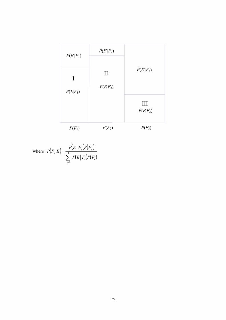
Instead of relying on tree diagrams, students may visualise Bayes’ Theorem as a ratio of
areas of rectangles by using an area model, which is basically a Venn diagram. For
example, the case of n = 3 can be represented by the area model on next page:
B2
B3
Bi B1
Bn
A
25
where
3
1iii
jj
j
FPFEP
FPFEPEFP
P(EF1)
P(EF1)
P(EF3)
P(EF3)
P(EF2)
P(EF2)
P(F1) P(F2) P(F3)
I II
III
26
Learning Unit Learning Objective Time
Statistics Area
Binomial, Geometric and Poisson Distributions
12. Discrete random
variables
12.1 recognise the concept of a discrete random
variable
1
Explanatory Notes:
Teachers may explain the concept of random experiments before introducing random
variables. An experiment can be considered as random if it satisfies the following
conditions:
(i) The experiment can be performed repeatedly under the same condition(s)
(ii) All possible outcomes of the experiment are obtainable and there are more than one
possible outcome
(iii) The outcome of the experiment is unknown before the experiment
Teachers can introduce the preliminary idea of a random variable by using simple
examples such as tossing of coins (for discrete random variables) and life times of electric
bulbs (for continuous random variables).
27
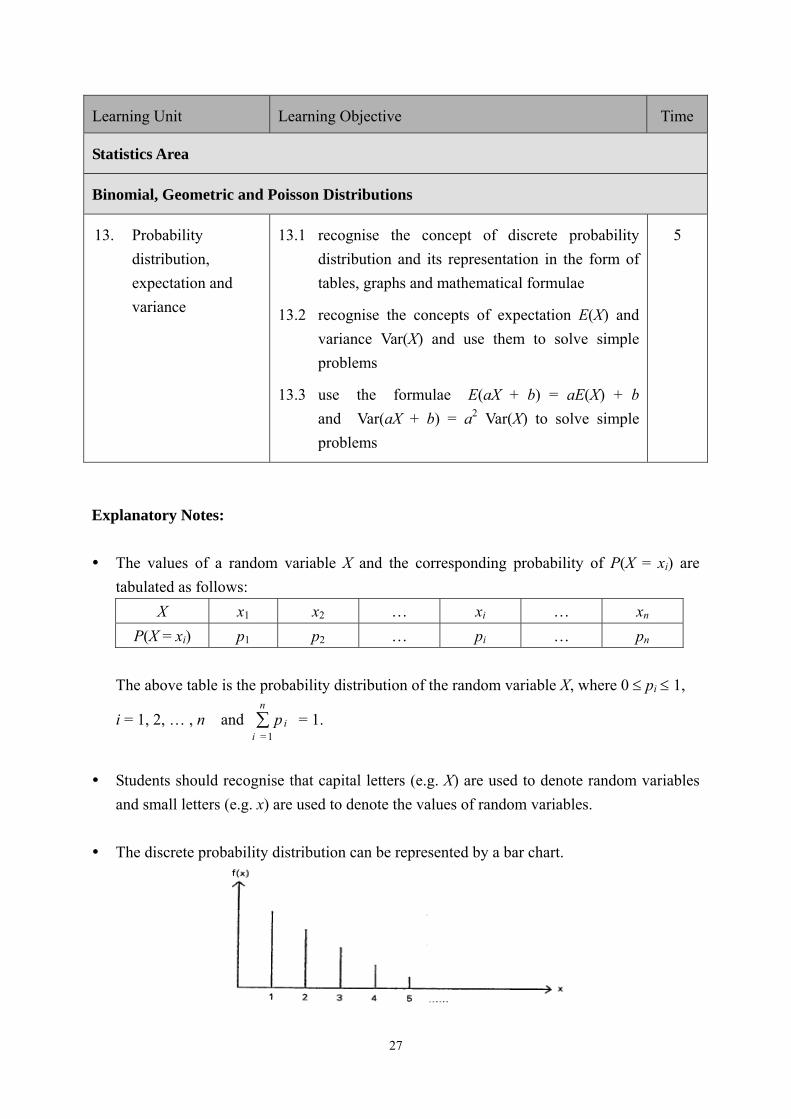
Learning Unit Learning Objective Time
Statistics Area
Binomial, Geometric and Poisson Distributions
13. Probability
distribution,
expectation and
variance
13.1 recognise the concept of discrete probability
distribution and its representation in the form of
tables, graphs and mathematical formulae
13.2 recognise the concepts of expectation E(X) and
variance Var(X) and use them to solve simple
problems
13.3 use the formulae E(aX + b) = aE(X) + b
and Var(aX + b) = a2 Var(X) to solve simple
problems
5
Explanatory Notes:
The values of a random variable X and the corresponding probability of P(X = xi) are
tabulated as follows:
X x1 x2 … xi … xn
P(X = xi) p1 p2 … pi … pn
The above table is the probability distribution of the random variable X, where 0 pi 1,
i = 1, 2, … , n and i = 1
n
pi = 1.
Students should recognise that capital letters (e.g. X) are used to denote random variables
and small letters (e.g. x) are used to denote the values of random variables.
The discrete probability distribution can be represented by a bar chart.
28
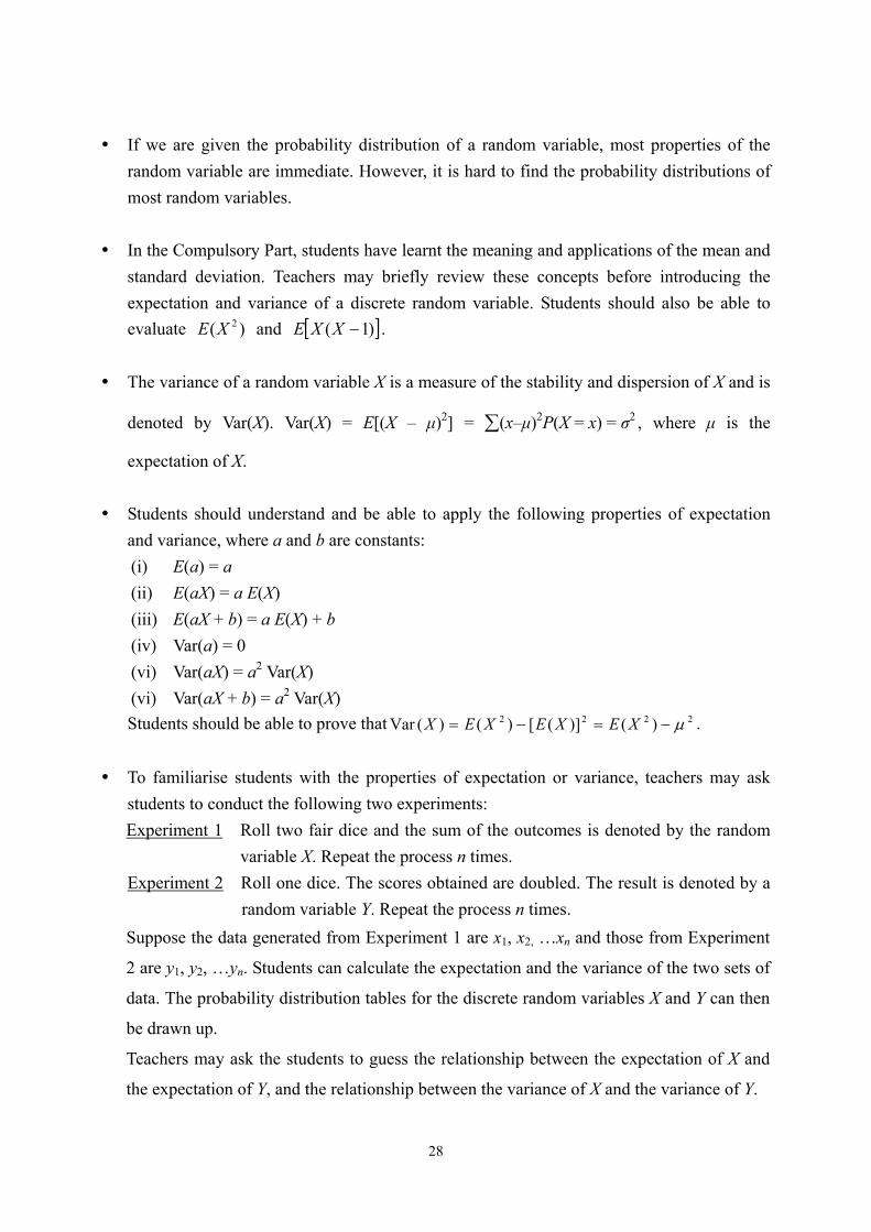
If we are given the probability distribution of a random variable, most properties of the
random variable are immediate. However, it is hard to find the probability distributions of
most random variables.
In the Compulsory Part, students have learnt the meaning and applications of the mean and
standard deviation. Teachers may briefly review these concepts before introducing the
expectation and variance of a discrete random variable. Students should also be able to
evaluate )( 2XE and )1( XXE .
The variance of a random variable X is a measure of the stability and dispersion of X and is
denoted by Var(X). Var(X) = E[(X – μ)2] = (x–μ)2P(X = x) = σ2 , where μ is the
expectation of X.
Students should understand and be able to apply the following properties of expectation
and variance, where a and b are constants:
(i) E(a) = a
(ii) E(aX) = a E(X)
(iii) E(aX + b) = a E(X) + b
(iv) Var(a) = 0
(vi) Var(aX) = a2 Var(X)
(vi) Var(aX + b) = a2 Var(X)
Students should be able to prove that 2222 )()]([)()(Var XEXEXEX .
To familiarise students with the properties of expectation or variance, teachers may ask
students to conduct the following two experiments:
Experiment 1 Roll two fair dice and the sum of the outcomes is denoted by the random
variable X. Repeat the process n times.
Experiment 2 Roll one dice. The scores obtained are doubled. The result is denoted by a
random variable Y. Repeat the process n times.
Suppose the data generated from Experiment 1 are x1, x2, …xn and those from Experiment
2 are y1, y2, …yn. Students can calculate the expectation and the variance of the two sets of
data. The probability distribution tables for the discrete random variables X and Y can then
be drawn up.
Teachers may ask the students to guess the relationship between the expectation of X and
the expectation of Y, and the relationship between the variance of X and the variance of Y.
29
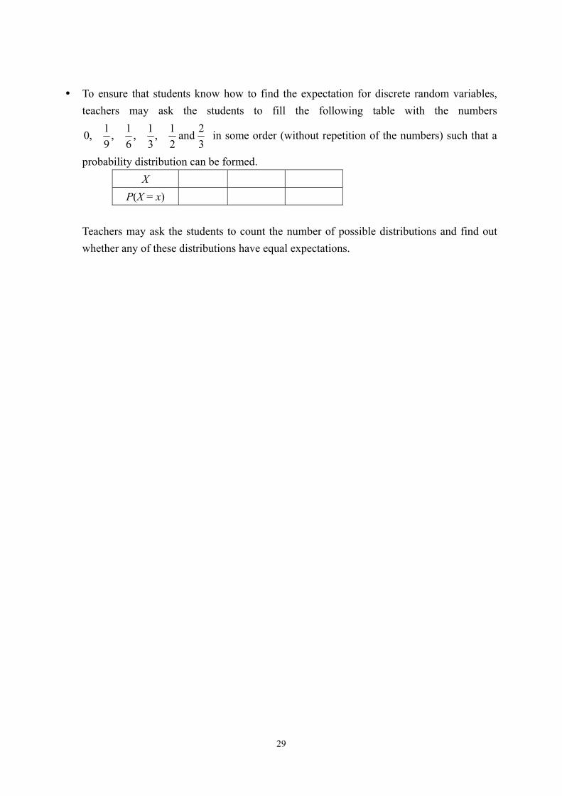
To ensure that students know how to find the expectation for discrete random variables,
teachers may ask the students to fill the following table with the numbers
3
2and
2
1,
3
1,
6
1,
9
1,0 in some order (without repetition of the numbers) such that a
probability distribution can be formed.
X
P(X = x)
Teachers may ask the students to count the number of possible distributions and find out
whether any of these distributions have equal expectations.
30
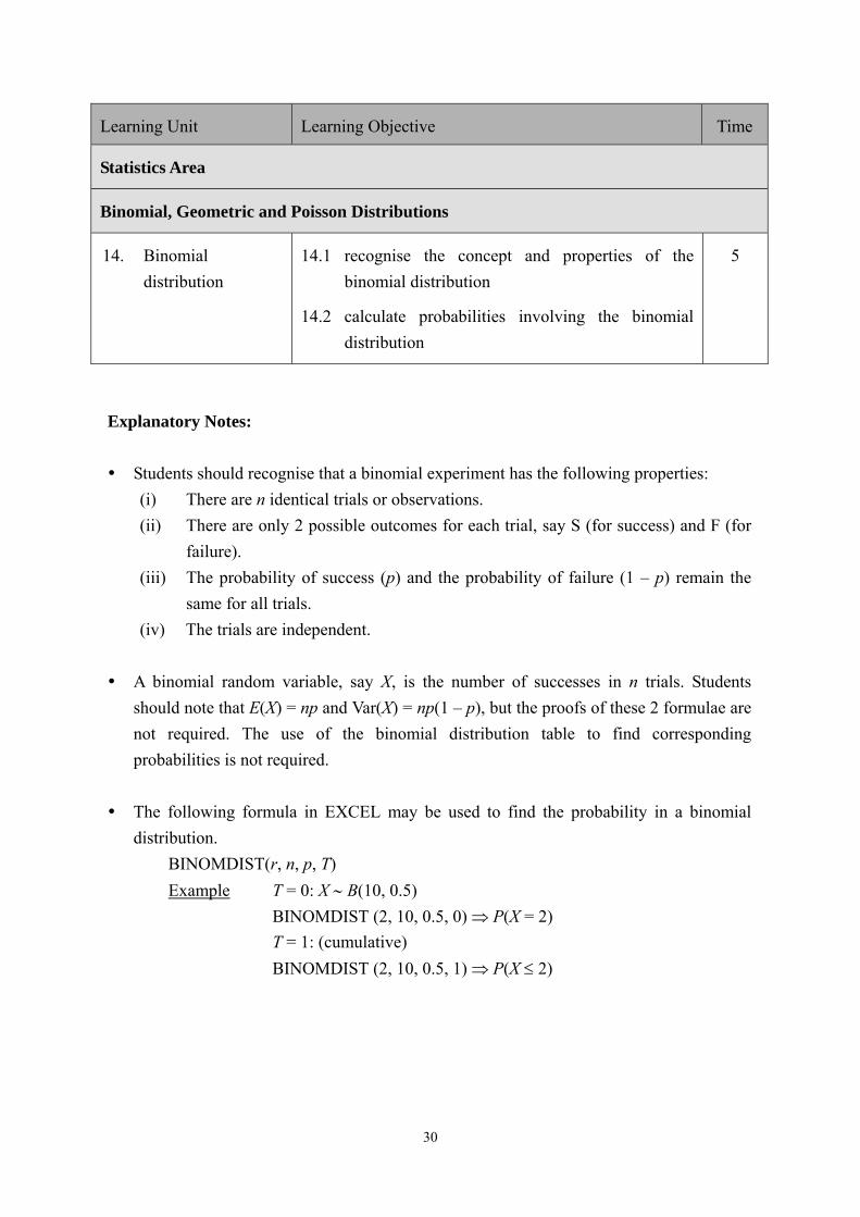
Learning Unit Learning Objective Time
Statistics Area
Binomial, Geometric and Poisson Distributions
14. Binomial
distribution
14.1 recognise the concept and properties of the
binomial distribution
14.2 calculate probabilities involving the binomial
distribution
5
Explanatory Notes:
Students should recognise that a binomial experiment has the following properties:
(i) There are n identical trials or observations.
(ii) There are only 2 possible outcomes for each trial, say S (for success) and F (for
failure).
(iii) The probability of success (p) and the probability of failure (1 – p) remain the
same for all trials.
(iv) The trials are independent.
A binomial random variable, say X, is the number of successes in n trials. Students
should note that E(X) = np and Var(X) = np(1 – p), but the proofs of these 2 formulae are
not required. The use of the binomial distribution table to find corresponding
probabilities is not required.
The following formula in EXCEL may be used to find the probability in a binomial
distribution.
BINOMDIST(r, n, p, T)
Example T = 0: X B(10, 0.5)
BINOMDIST (2, 10, 0.5, 0) P(X = 2)
T = 1: (cumulative)
BINOMDIST (2, 10, 0.5, 1) P(X 2)
31
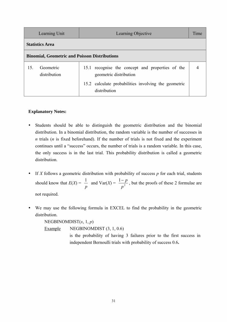
Learning Unit Learning Objective Time
Statistics Area
Binomial, Geometric and Poisson Distributions
15. Geometric
distribution
15.1 recognise the concept and properties of the
geometric distribution
15.2 calculate probabilities involving the geometric
distribution
4
Explanatory Notes:
Students should be able to distinguish the geometric distribution and the binomial
distribution. In a binomial distribution, the random variable is the number of successes in
n trials (n is fixed beforehand). If the number of trials is not fixed and the experiment
continues until a “success” occurs, the number of trials is a random variable. In this case,
the only success is in the last trial. This probability distribution is called a geometric
distribution.
If X follows a geometric distribution with probability of success p for each trial, students
should know that E(X) = p
1 and Var(X) =
2
1
p
p, but the proofs of these 2 formulae are
not required.
We may use the following formula in EXCEL to find the probability in the geometric
distribution.
NEGBINOMDIST(x, 1, p)
Example NEGBINOMDIST (3, 1, 0.6)
is the probability of having 3 failures prior to the first success in
independent Bernoulli trials with probability of success 0.6.
32
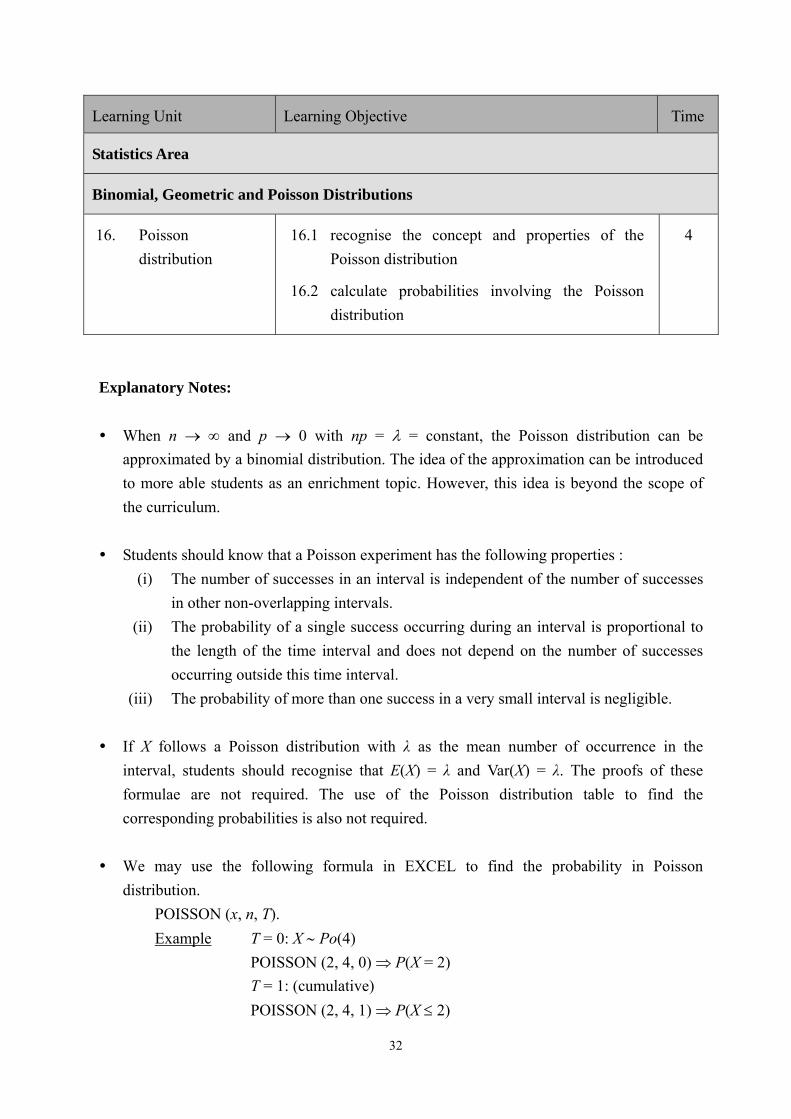
Learning Unit Learning Objective Time
Statistics Area
Binomial, Geometric and Poisson Distributions
16. Poisson
distribution
16.1 recognise the concept and properties of the
Poisson distribution
16.2 calculate probabilities involving the Poisson
distribution
4
Explanatory Notes:
When n and p 0 with np = = constant, the Poisson distribution can be
approximated by a binomial distribution. The idea of the approximation can be introduced
to more able students as an enrichment topic. However, this idea is beyond the scope of
the curriculum.
Students should know that a Poisson experiment has the following properties :
(i) The number of successes in an interval is independent of the number of successes
in other non-overlapping intervals.
(ii) The probability of a single success occurring during an interval is proportional to
the length of the time interval and does not depend on the number of successes
occurring outside this time interval.
(iii) The probability of more than one success in a very small interval is negligible.
If X follows a Poisson distribution with λ as the mean number of occurrence in the
interval, students should recognise that E(X) = λ and Var(X) = λ. The proofs of these
formulae are not required. The use of the Poisson distribution table to find the
corresponding probabilities is also not required.
We may use the following formula in EXCEL to find the probability in Poisson
distribution.
POISSON (x, n, T).
Example T = 0: X Po(4)
POISSON (2, 4, 0) P(X = 2)
T = 1: (cumulative)
POISSON (2, 4, 1) P(X 2)
33
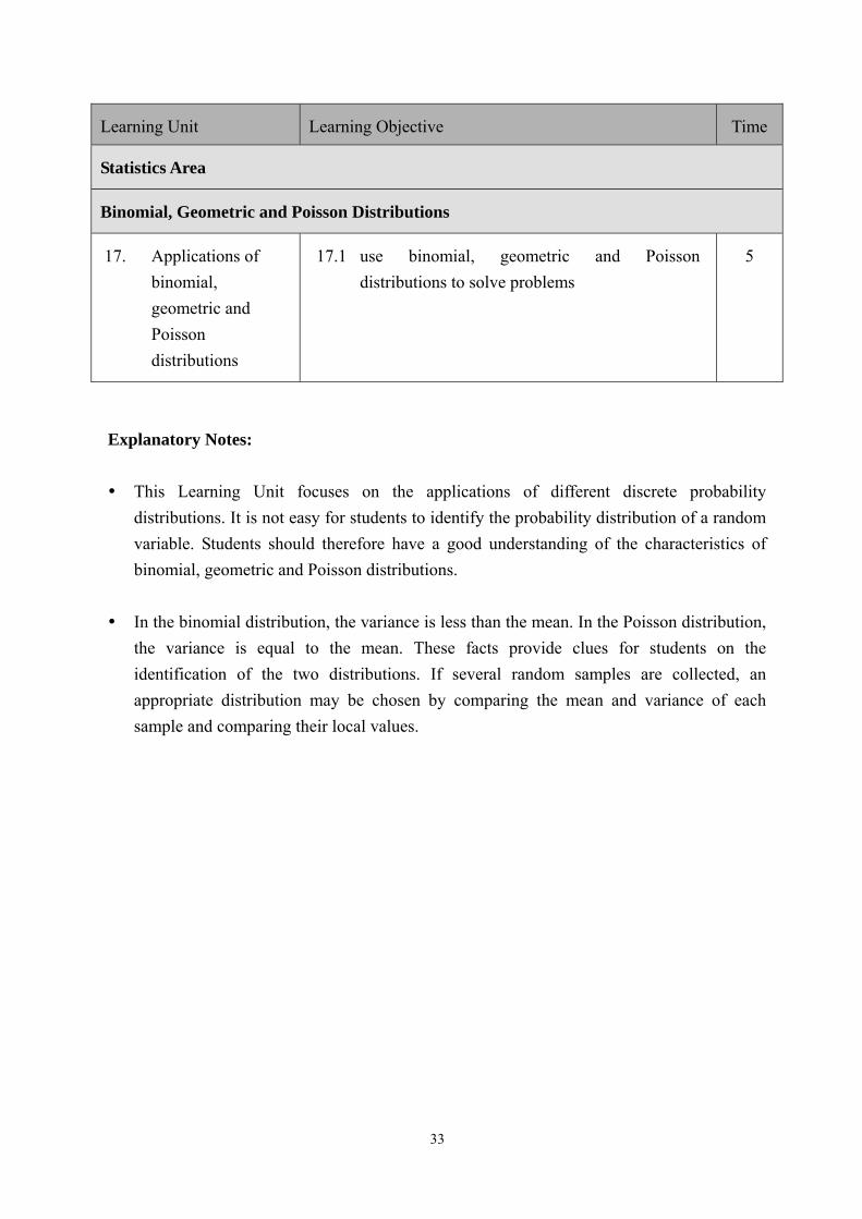
Learning Unit Learning Objective Time
Statistics Area
Binomial, Geometric and Poisson Distributions
17. Applications of
binomial,
geometric and
Poisson
distributions
17.1 use binomial, geometric and Poisson
distributions to solve problems
5
Explanatory Notes:
This Learning Unit focuses on the applications of different discrete probability
distributions. It is not easy for students to identify the probability distribution of a random
variable. Students should therefore have a good understanding of the characteristics of
binomial, geometric and Poisson distributions.
In the binomial distribution, the variance is less than the mean. In the Poisson distribution,
the variance is equal to the mean. These facts provide clues for students on the
identification of the two distributions. If several random samples are collected, an
appropriate distribution may be chosen by comparing the mean and variance of each
sample and comparing their local values.
34
Learning Unit Learning Objective Time
Statistics Area
Normal Distribution
18. Basic definition
and properties
18.1 recognise the concepts of continuous random
variables and continuous probability
distributions, with reference to the normal
distribution
18.2 recognise the concept and properties of the
normal distribution
3
Explanatory Notes:
Students should know the difference between the probability distribution of a discrete
random variable and the probability distribution of a continuous random variable.
The proofs of E(X) = ∞
–∞x f (x) dx = μ and Var(X) =
∞
–∞(x- μ)2
f (x) dx = σ2 are
not required. However, students should know that the formulae E(aX+b) = aE(X) + b
and Var(aX + b) = a2Var(X) also apply to continuous random variables.
35
Learning Unit Learning Objective Time
Statistics Area
Normal Distribution
19. Standardisation
of a normal
variable and use
of the standard
normal table
19.1 standardise a normal variable and use the
standard normal table to find probabilities
involving the normal distribution.
2
Explanatory Notes:
The statement “X follows a normal distribution with mean and variance 2 ” may be
represented by X N(,2)
The standard normal distribution is a special case of the normal distribution with 0
and 1 and is denoted by X N(0,1).
Students should know that if X ~ N(, 2) and
X
Z , then
(i) Z ~ N(0, 1)
(ii) E(Z) = 0 and Var(Z) = 1
(iii) )()() 21 zZzPbXa
PbXP(a
Students are expected to use the standard normal table to find values like P(Z > a),
P(Z b) and P(a Z b).
The following normal distribution formulae are available in EXCEL:
NORMDIST (x, , σ, T): For X ~ N(, σ2), when T = 1, we get P(X x)
NORMINV(p, , σ): For X ~ N(, σ2), we get the value of x such that P(X x) = p
NORMSDIST(z): For Z ~ N(0,1), we get P(Z z)
NORMSINV(p): We get z such that P(Z z) = p
STANDARDIZE (x, , σ): We get -x
Z
36
Learning Unit Learning Objective Time
Statistics Area
Normal Distribution
20. Applications of
the normal
distribution
20.1 find the values of )( 1xXP , )( 2xXP ,
)( 21 xXxP and related probabilities, given
the values of x1, x2, and , where
X ~ N(, σ2)
20.2 find the values of x, given the values of
P(X > x), P(X < x), P(a < X < x), P(x < X < b) or
a related probability, where X ~ N(, σ2)
20.3 use the normal distribution to solve problems
7
Explanatory Notes:
Students do not need to recognise that the sum of scalar multiples of independent normal
variables is also normal. For example, if X1 ~ N(8, 32), X2 ~ N(12, 42) and X1 and X2 are
independent, students are not expected to know that the distribution of Y = X1 + X2 is
normal and Y ~ N(20, 52).
37
Learning Unit Learning Objective Time
Statistics Area
Point and Interval Estimation
21. Sampling
distribution and
point estimates
21.1 recognise the concepts of sample statistics and
population parameters
21.2 recognise the sampling distribution of the
sample mean from a random sample of size n
21.3 recognise the concept of point estimates
including the sample mean, sample variance and
sample proportion
21.4 recognise Central Limit Theorem
7
Explanatory Notes:
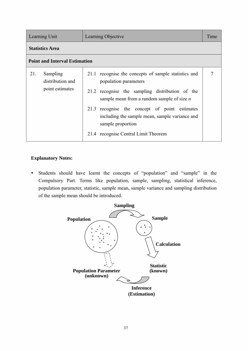
Students should have learnt the concepts of “population” and “sample” in the
Compulsory Part. Terms like population, sample, sampling, statistical inference,
population parameter, statistic, sample mean, sample variance and sampling distribution
of the sample mean should be introduced.
Population Parameter(unknown)
Statistic(known)
Population Sample
Sampling
Inference (Estimation)
Calculation
38
Students are expected to know the following formulae:
(i) sample mean
k
iii xf
nx
1
1, where
k
iifn
1
(ii) sample variance 2
1
2
1
1xxf
ns i
k
ii
, where
k
iifn
1
(iii) The values of the sample mean x and sample variance s2 will be respectively
close to the population mean μ and population variance σ2 when the sample size is
sufficiently large.
(iv) For a finite population, population variance
k
iii xf
N 1
22 1 , where N is the
population size.
Teachers may conduct some sampling activities and discuss with students:
(i) The meaning of the mean of the sample means and the variance of the sample
means.
(ii) If the population is normally distributed with mean and variance 2 , the mean
of the sample means is normally distributed with mean and variance n
2.
(iii) The sampling distribution of the sample means approaches a normal distribution
when n is sufficiently large. The population concerned is not necessarily normal.
The following points might be highlighted in class:
(i) A sample statistic is not necessarily the same as the corresponding population
parameter, but it can provide good information about that parameter.
(ii) Most sample statistics are close to the population parameters. Few are extremely
larger or smaller than the corresponding population value.
(iii) The goodness of a particular estimate is directly dependent on the size of the
sample. In general, samples that are larger produce statistics that vary less from the
population value.
Point estimation is one of the methods of parameter estimation. It is worthwhile, at this
stage, for teachers to introduce the concept of estimation of an unknown population
parameter from a sample statistic. Examples like estimating a population mean μ by
using a sample mean x can be used for illustration. Teachers should indicate to
students that there may be several sample statistics which can be used as estimators. For
example, the sample mean, sample median and sample mode could also be used to
estimate the population mean μ.
39
In the process of sampling, different estimates are obtained from different samples. It is
difficult to determine which estimator is the most suitable one. We may use the unbiased
estimator to estimate the unknown parameter. It is expected that, in the long run, the
average value of our estimates taken over a large number of samples should equal the
population value: E(sample estimator) = population parameter. Teachers may show that
X is an unbiased estimator of the population mean , but
n
iix XX
n 1
22 1 is
not an unbiased estimator of the population variance 2 . Hence, students should
use
n
ii XX
ns
1
22
1
1, as an unbiased estimator of the population variance.
Central Limit Theorem is one of the most important and useful concepts in Statistics. It
states that, given a distribution with a mean μ and a variance 2 , the sampling
distribution of the mean will be approximately normally distributed with mean μ and
variancen
2when n (the sample size) is sufficiently large. However, the concept is too
abstract for students. Teachers may use the interactive and simulation programmes on
the Internet to illustrate the theorem.
By simulation programmes, students may note that:
(i) no matter what the shape of the original distribution is, the sampling distribution of
the mean approaches a normal distribution as the sample size increases
(ii) Most distributions approach a normal distribution very quickly as the sample size
increases
(iii) the number of samples is assumed to be infinite in a sampling distribution
(iv) the spread of the distributions decreases as the sample size increases
40
Learning Unit Learning Objective Time
Statistics Area
Point and Interval Estimation
22. Confidence
interval for a
population mean
22.1 recognise the concept of confidence interval
22.2 find the confidence interval for a population
mean
6
Explanatory Notes:
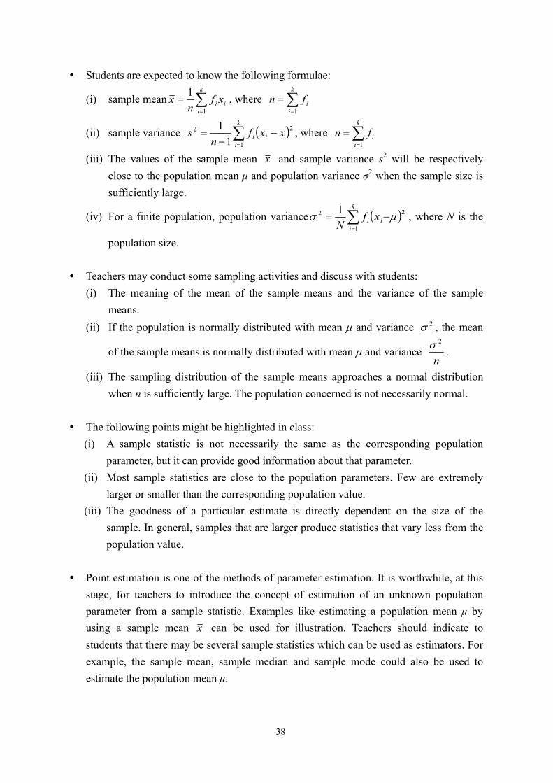
A confidence interval for a population mean is an
interval estimate of an unknown population
parameter , based on a random sample from the
population. The confidence interval is an abstract
concept. Teachers may illustrate its meaning by
computer simulation programmes or statistical
software such as Winstat.
Teachers should point out that the confidence interval is derived from random samples.
95% confidence interval and the 99% confidence interval are most commonly used.
Before constructing a confidence interval for , it is essential to ask the following
questions:
Are the random samples taken from a normal population?
Is the population variance known?
Is the sample size large enough?
For a normal population, based on a sample of size n, the 95% confidence interval for
the population mean with known variance 2 is ( x –1.96
n), x + 1.96
n).
If X N( , 2), then —X ~
n
N2
, and 0.95 = P(–1.96 ≤ Z ≤ 1.96) =
P(–1.96 ≤ —X –/ n
≤ 1.96). It should be noted that the results are true for samples of any
sizes.
41
For a non-normal population, the 95% confidence interval for the population mean
with a known variance σ2 and large n (say, n 30) is
nx
nx
96.1 ,.961 . As
the sample size is large, Central Limit Theorem can be used. X is approximately
normal and —X ~
n
N2
, .
For a normal or non-normal population, the 95% confidence interval for the population
mean with unknown variance 2 and large n (say, n 30) is
n
sx
n
sx 96.1 ,.961 , where s2 represents the sample variance and
95.096.1≤≤96.1
ns
XP
, where n
s is called the standard error of the sample
and is denoted by SE( x ).
Students should be able to evaluate the confidence interval for the population mean μ
under the following situations:
Conditions 95% confidence
interval for μ
99% confidence
interval for μ
Normal population
with known variance σ2
large or small sample size n
sample mean x
(x̄ 1.96n , x̄ + 1.96
n
) (x̄ 2.575n
, x̄ + 2.575n)
Non-normal population
with known variance σ2
large sample size n (n 30)
sample mean x
(x̄ 1.96n , x̄ + 1.96
n
) (x̄ 2.575n
, x̄ + 2.575n)
Non-normal population
with unknown variance σ2
large sample size n (n 30)
sample mean x
sample variance 2s
(x̄ 1.96sn , x̄ + 1.96
sn
) (x̄ 2.575sn
, x̄ + 2.575sn)
Students should know that the width of the confidence interval can be reduced:
by increasing the sample size
by decreasing the confidence level (e.g. choosing a confidence level of 95% instead
of 99%)

42
In constructing a confidence interval, it is desirable to have a narrow width (for a more
precise estimate) with a high level of confidence, but in most cases, we cannot attain
these two conditions at the same time.
If random samples are independently taken from a population and 95% confidence
intervals constructed for each sample, students may expect about 5% of the intervals do
not include the population parameter. When students calculate their confidence intervals,
they will not know whether the parameter is included in these intervals or not.
43
Learning Unit Learning Objective Time
Statistics Area
Point and Interval Estimation
23. Confidence
interval for a
population
proportion
23.1 find an approximate confidence interval for a
population proportion
3
Explanatory Notes:
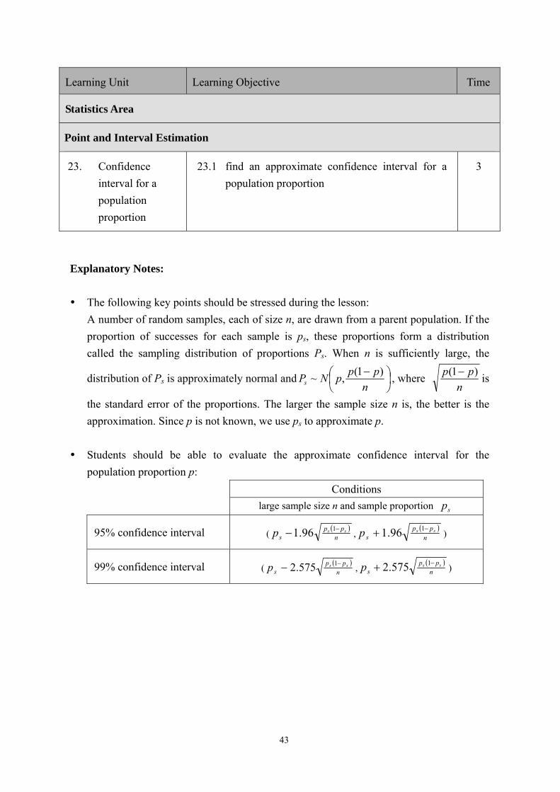
The following key points should be stressed during the lesson:
A number of random samples, each of size n, are drawn from a parent population. If the
proportion of successes for each sample is ps, these proportions form a distribution
called the sampling distribution of proportions Ps. When n is sufficiently large, the
distribution of Ps is approximately normal and
n
pppNPs
)1(,~ , where
n
pp )1( is
the standard error of the proportions. The larger the sample size n is, the better is the
approximation. Since p is not known, we use ps to approximate p.
Students should be able to evaluate the approximate confidence interval for the
population proportion p:
Conditions
large sample size n and sample proportion sp
95% confidence interval (
npp
sssp 196.1 ,
n
pps
ssp 196.1 )
99% confidence interval (
n
pps
ssp 1575.2 ,
npp
sssp 1575.2 )
44
Learning Unit Learning Objective Time
Further Learning Unit
24. Inquiry and
investigation
Through various learning activities, discover and
construct knowledge, further improve the ability to
inquire, communicate, reason and conceptualise
mathematical concepts
10
Explanatory Notes:
This Learning Unit aims at providing students with more opportunities to engage in the
activities that avail themselves of discovering and constructing knowledge, further
improving their abilities to inquire, communicate, reason and conceptualise mathematical
concepts when studying other Learning Units. In other words, this is not an independent and
isolated Learning Unit and the activities may be conducted in different stages of a lesson,
such as motivation, development, consolidation or assessment.

45
Acknowledgements
We would like to thank the members of the following Committees and Working Group for
their invaluable comments and suggestions in the compilation of this booklet.
CDC Committee on Mathematics Education
CDC-HKEAA Committee on Mathematics Education (Senior Secondary)
CDC-HKEAA Working Group on Senior Secondary Mathematics Curriculum (Module 1)