explaining cointegration analysis: part ii · pdf fileexplaining cointegration analysis: part...
TRANSCRIPT

Explaining Cointegration Analysis: Part II
David F. Hendry and Katarina Juselius
Nuffield College, Oxford, OX1 1NF.Department of Economics, University of Copenhagen, Denmark
Abstract We describe the concept of cointegration, its implications in modelling and forecasting, and discussinference procedures appropriate in integrated-cointegrated vector autoregressive processes (VARs). Particularattention is paid to the properties of VARs, to the modelling of deterministic terms, and to the determination of thenumber of cointegration vectors. The analysis is illustrated by empirical examples.
1. Introduction
Hendry and Juselius (2000) investigated the properties of economic time series that were integratedprocesses, such as random walks, which contained a unit root in their dynamics. Here we extend theanalysis to the multivariate context, and focus on cointegration in systems of equations.
We showed in Hendry and Juselius (2000) that when data were non-stationary purely due to unitroots (integrated once, denotedI(1)), they could be brought back to stationarity by the linear trans-formation of differencing, as inxt − xt−1 = ∆xt. For example, if the data generation process (DGP)were the simplest random walk with an independent normal (IN) error having mean zero and constantvarianceσ2
ε :xt = xt−1 + εt where εt ∼ IN
[0, σ2
ε
], (1)
then subtractingxt−1 from both sides delivers∆xt ∼ IN[0, σ2
ε
]which is certainly stationary.1 Since
∆xt cannot have a unit root, it must beI(0). Such an analysis generalizes to (say) twice-integratedseries – which areI(2)– so must becomeI(0) after differencing twice.
It is natural to enquire if other linear transformations than differencing will also induce stationarity.The answer is ‘possibly’, but unlike differencing, there is no guarantee that the outcome must beI(0):cointegration analysis is designed to find linear combinations of variables that also remove unit roots.In a bivariate context, ifyt andxt are bothI(1), there may (but need not) be a unique value ofβ such thatyt − βxt is I(0): in other words, there is no unit root in the relation linkingyt andxt. Consequently,cointegration is a restriction on a dynamic model, and so is testable. Cointegration vectors are ofconsiderable interest when they exist, since they determineI(0) relations that hold between variableswhich are individually non-stationary. Such relations are often called ‘long-run equilibria’, since it canbe proved that they act as ‘attractors’ towards which convergence occurs whenever there are departurestherefrom (see e.g., Granger (1986), and Banerjee, Dolado, Galbraith, and Hendry (1993), ch. 2).
Since I(1) variables ‘wander’ (often quite widely) because of their stochastic trends, whereas(weakly) stationary variables have constant means and variances, if there exists a linear combination
1Notice that differencing is not anoperatorfor equations: one can difference data (to create∆xt), but attempting to differ-ence equation (1) would lead to∆xt = ∆xt−1 + ∆εt. Such an equation is not well defined, since∆ can be cancelled on bothsides, so is redundant.

2 David F. Hendry and Katarina Juselius
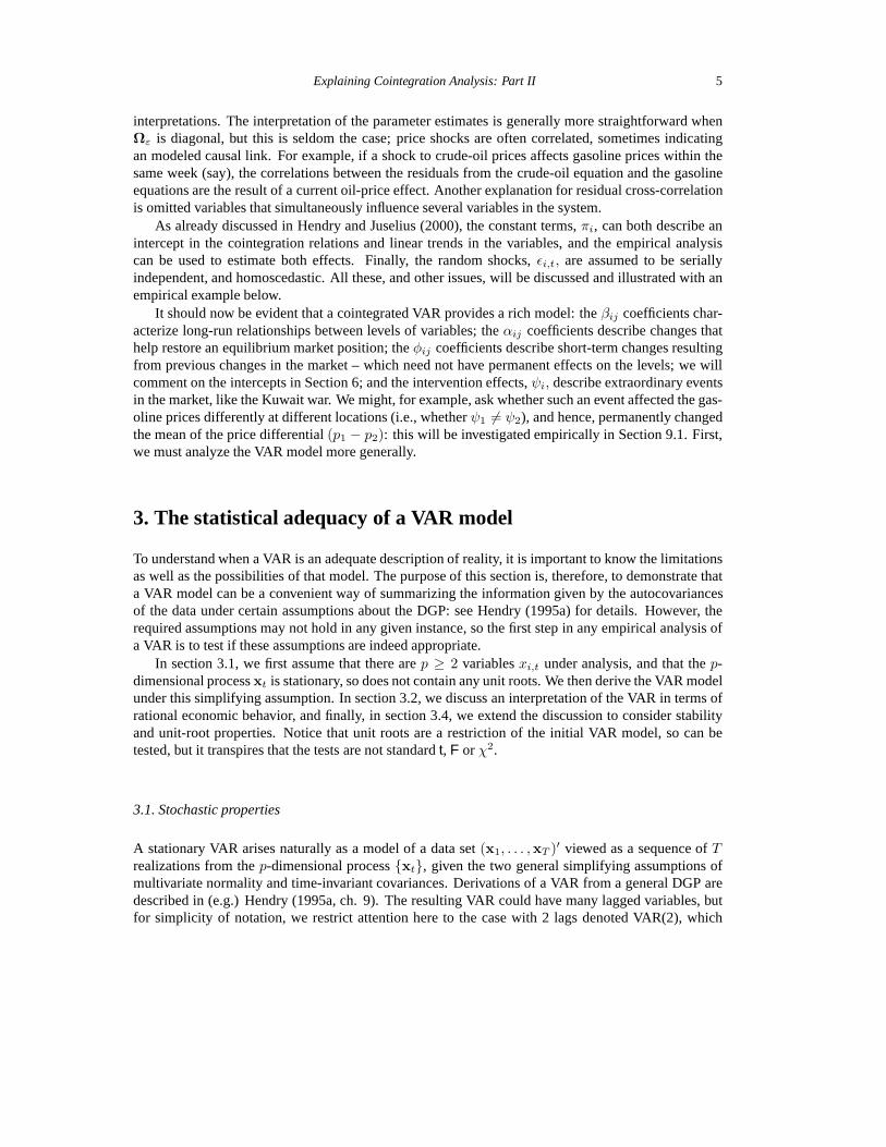
that delivers anI(0) relation, it might be thought that it would be obvious from graphs of the variables.Unfortunately, that need not be the case, as figure 1 shows. In panel a, three variables (denotedya, yb,yc) are plotted that are actually very strongly cointegrated, whereas panel b plots another two (denotedYa, Yb) that are neither cointegrated, nor linked in any causal way. Panels c and d respectively show thechanges in these variables. It is not obvious from the graphs that the first set are closely linked whereasthe second are not connected at all. Nevertheless, thePcGivecointegration test, described in Hendryand Juselius (2000), applied to simple dynamic models relatingya to yb andyc, andYa to Yb, respect-ively takes the valuestur = −6.25∗∗ andtur = −2.31, so the first strongly rejects a unit root in therelation, whereas the second does not. Thus, cointegration may or may not exist between variables thatdo or do not ‘look cointegrated’, and the only way to find out is through a careful statistical analysis,rather than rely on visual inspection. These two points, namely the importance but non-obvious natureof cointegrated relations, motivates our discussion.
0 50 100 150 200
−2.5
0
2.5
5
7.5ya yb yc
0 50 100 150 200
2
4
6 Ya Yb
0 50 100 150 200
−.5
0
.5
∆ya ∆yb ∆yc
0 50 100 150 200
−.2
0
.2
∆Ya ∆Yb
Figure 1. Cointegrated and non-cointegrated time series
The organization of this paper is as follows. Section 2 begins by illustrating the inherently mul-tivariate nature of cointegration analysis: several variables must be involved, and this determines theform of the statistical tools required. Section 3 then discusses the conditions under which a vectorautoregressive process (VAR) would provide a feasible empirical model for integrated economic timeseries, spelling out both its statistical and economic requirements, illustrated by the empirical exampleused in Hendry and Juselius (2000). In section 4, we consider alternative representations of the VARthat yield different insights into its properties under stationarity, and also set the scene for derivingthe necessary and sufficient conditions that deliver an integrated-cointegrated process. The purpose ofsection 5 is to define cointegration via restrictions on the VAR model, and relate the properties of thevector process to stochastic trends and stationary components based on the moving-average representa-

Explaining Cointegration Analysis: Part II 3
tion. Section 6 considers the key role of deterministic terms (like constants and trends) in cointegrationanalyses.
At that stage, the formalization of the model and analysis of its properties are complete, so weturn to issues of estimation (section 7) and inference (section 8), illustrated empirically in section 9.Section 10 considers the identification of the cointegration parameters, and hypothesis tests thereon,and section 11 discusses issues that arise in the analysis of partial systems (conditional on a subsetof the variables) and the closely related concept of exogeneity. Finally, we discuss forecasting incointegrated systems (section 12) and the associated topic of parameter constancy (section 13), alsorelevant to any policy applications of cointegrated systems. Section 14 concludes. The paper usesmatrix algebra extensively to explain the main ideas, so we adopt the following notation: bold-facecapital letters for matrices, bold-face lower case for vectors, normal case for variables and coefficients,and Greek letters for parameters. We generally assume all variables are in logs, which transformationproduces more homogeneous series for inherently-positive variables (see e.g., Hendry (1995a), ch. 2),but we will not distinguish explicitly between logs and the original units.2
2. The multivariate nature of cointegration analysis
Cointegration analysis is inherently multivariate, as a single time series cannot be cointegrated. Con-sequently, consider a set of integrated variables, such as gasoline prices at different locations as inHendry and Juselius (2000), where each individual gasoline price (denotedpi,t) is I(1), but follows acommon long-run path, affected by the world price of oil (po,t). Cointegration between the gasolineprices could arise, for example, if the price differentials between any two locations were stationary.However, cointegration as such does not say anything about the direction of causality. For example,one of the locations could be a price leader and the others price followers; or, alternatively, none of thelocations might be more important than the others. In the first case, the price of the leading locationwould be driving the prices of the other locations (be ‘exogenous’ to the other prices) and cointegrationcould be analyzed from the equations for the other ‘adjusting’ prices, given the price of the leader. Inthe second case, all prices would be ‘equilibrium adjusting’ and, hence, all equations would contain in-formation about the cointegration relationships. In the bivariate analysis in Hendry and Juselius (2000),cointegration was found in a single-equation model ofp1,t givenp2,t, thereby assuming thatp2,t wasa price leader. If this assumption was incorrect, then the estimates of the cointegration relation wouldbe inefficient, and could be seriously biased. To find out which variables adjust, and which do notadjust, to the long-run cointegration relations, an analysis of the full system of equations is required,as illustrated in Section 11.
Here, we will focus on a vector autoregression (VAR) as a description of the system to be investig-ated. In a VAR, each variable is ‘explained’ by its own lagged values, and the lagged values of all othervariables in the system. To see which questions can be asked within a cointegrated VAR, we postulate atrivariate VAR model for the two gasoline pricesp1,t andp2,t, together with the price of crude oil,po,t.We restrict the analysis to one lagged change for simplicity, and allow for 2 cointegration relations.
2If a variable had a unit root in its original units of measurement, it would become essentially deterministic over time if it hada constant error variance. Thus, absolute levels must have heteroscedastic errors to make sense; but if so, that is not a sensibleplace to start modeling. Moreover, if the log had a unit root, then the original must be explosive. Many economic variables seemto have that property, appearing to show quadratic trends in absolute levels.

4 David F. Hendry and Katarina Juselius
Then the system can be written as: ∆p1,t
∆p2,t
∆po,t
=
φ11 φ12 φ13
φ21 φ22 φ23
φ31 φ32 φ33
∆p1,t−1
∆p2,t−1
∆po,t−1
+
α11 α12
α21 α22
α31 α32
( (p1 − p2)t−1
(p2 − po)t−1
)
+
ψ1
ψ2
ψ3
d1,t +
π1
π2
π3
+
ε1,t
ε2,t
ε3,t
, (2)
whereεt is assumedIN3[0,Ωε], andΩε is the (positive-definite, symmetric) covariance matrix of theerror process.
Within the hypothetical system (2), we could explain the three price changes from periodt − 1(previous week) tot (this week) as a result of:
(i) an adjustment to previous price changes, with impactsφij for the jth lagged change in theith
equation;(ii) an adjustment to previous disequilibria between prices in different locations,(p1 − p2), and
between the price in location 2 and the price of crude oil,(p2 − po), with impactsαi1 andαi2
respectively in theith equation;(iii) an extraordinary intervention in the whole market, such as the outbreak of the Kuwait war, de-
scribed by the intervention dummyd1,t;(iv) a constant termπ; and(v) random shocks,εt.
When all three prices areI(1), whereas(p1,t − p2,t) and (p2,t − po,t) are I(0), then the latterdescribe cointegrated relations, i.e., relations that are stationary even when the variables themselvesare non-stationary. Cointegration between the prices means that the three prices follow the same long-run trends, which then cancel in the price differentials. This may seem reasonablea priori, but couldnevertheless be incorrect empirically: using multivariate cointegration analysis, we can formally testwhether such is indeed the case. In general, we write cointegration relations in the form:
β11p1,t + β12p2,t + β13po,t; and β21p1,t + β22p2,t + β32po,t (3)
etc., where, in (2), we have normalizedβ11 = β22 = 1, and setβ13 = β21 = 0. Such restrictionscannot be imposed arbitrarily in empirical research, so we will discuss how to test restrictions oncointegration relations in Section 10.
The existence of cointegration by itself does imply which prices ‘equilibrium adjust’ and whichdo not; nor does it entail whether any adjustment is fast or slow. Information about such features canbe provided by theαij coefficients. For example,α31 = α32 = 0, would tell us that there were nofeed-back effects onto the price of crude oil from ‘deviant’ price behavior in the gasoline market. Inthis case, the price of crude oil would influence gasoline prices, but would not be influenced by them.Next, consider, for example, whenα11 = −0.6 whereasα21 = −0.1. Then, gasoline prices at location1 adjust more quickly to restore an imbalance between its own price and the price at location 2 than theother way around. Finally, considerα22 = −0.4: then the location-2 price would adjust quite quicklyto changes in the level of crude oil price. In that case, we would be inclined to say that the price of crudeoil influenced the price of location 2 which influenced the price at location 1. This would certainly bethe case if the covariance matrixΩε was diagonal, so there were no contemporaneous links: ifΩε
was not diagonal, revealing cross-correlated residuals, one would have to be careful about ‘causal’
Explaining Cointegration Analysis: Part II 5
interpretations. The interpretation of the parameter estimates is generally more straightforward whenΩε is diagonal, but this is seldom the case; price shocks are often correlated, sometimes indicatingan modeled causal link. For example, if a shock to crude-oil prices affects gasoline prices within thesame week (say), the correlations between the residuals from the crude-oil equation and the gasolineequations are the result of a current oil-price effect. Another explanation for residual cross-correlationis omitted variables that simultaneously influence several variables in the system.
As already discussed in Hendry and Juselius (2000), the constant terms,πi, can both describe anintercept in the cointegration relations and linear trends in the variables, and the empirical analysiscan be used to estimate both effects. Finally, the random shocks,εi,t, are assumed to be seriallyindependent, and homoscedastic. All these, and other issues, will be discussed and illustrated with anempirical example below.
It should now be evident that a cointegrated VAR provides a rich model: theβij coefficients char-acterize long-run relationships between levels of variables; theαij coefficients describe changes thathelp restore an equilibrium market position; theφij coefficients describe short-term changes resultingfrom previous changes in the market – which need not have permanent effects on the levels; we willcomment on the intercepts in Section 6; and the intervention effects,ψi, describe extraordinary eventsin the market, like the Kuwait war. We might, for example, ask whether such an event affected the gas-oline prices differently at different locations (i.e., whetherψ1 6= ψ2), and hence, permanently changedthe mean of the price differential(p1 − p2): this will be investigated empirically in Section 9.1. First,we must analyze the VAR model more generally.
3. The statistical adequacy of a VAR model
To understand when a VAR is an adequate description of reality, it is important to know the limitationsas well as the possibilities of that model. The purpose of this section is, therefore, to demonstrate thata VAR model can be a convenient way of summarizing the information given by the autocovariancesof the data under certain assumptions about the DGP: see Hendry (1995a) for details. However, therequired assumptions may not hold in any given instance, so the first step in any empirical analysis ofa VAR is to test if these assumptions are indeed appropriate.
In section 3.1, we first assume that there arep ≥ 2 variablesxi,t under analysis, and that thep-dimensional processxt is stationary, so does not contain any unit roots. We then derive the VAR modelunder this simplifying assumption. In section 3.2, we discuss an interpretation of the VAR in terms ofrational economic behavior, and finally, in section 3.4, we extend the discussion to consider stabilityand unit-root properties. Notice that unit roots are a restriction of the initial VAR model, so can betested, but it transpires that the tests are not standardt, F or χ2.
3.1. Stochastic properties
A stationary VAR arises naturally as a model of a data set(x1, . . . ,xT )′ viewed as a sequence ofTrealizations from thep-dimensional processxt, given the two general simplifying assumptions ofmultivariate normality and time-invariant covariances. Derivations of a VAR from a general DGP aredescribed in (e.g.) Hendry (1995a, ch. 9). The resulting VAR could have many lagged variables, butfor simplicity of notation, we restrict attention here to the case with 2 lags denoted VAR(2), which

6 David F. Hendry and Katarina Juselius
suffices to illustrate all the main properties – and problems (the results generalize easily, but lead tomore cumbersome notation). We write the simplest VAR(2) as:
xt = π + Π1xt−1 + Π2xt−2 + εt (4)
whereεt ∼ INp [0,Ωε] , (5)
t = 1, . . . , T and the parameters(π,Π1,Π2,Ωε) are constant and unrestricted, except forΩε beingpositive-definite and symmetric.
Given (4), the conditional mean ofxt is:
E [xt | xt−1,xt−2] = π + Π1xt−1 + Π2xt−2 = mt,
say, and the deviation ofxt from mt definesεt:
xt − mt = εt.
Hence, if the assumptions of multivariate normality, time-constant covariances, and truncation at lag2are correct, then (4):
• is linear in the parameters;• has constant parameters;• has normally distributed errorsεt, with:• (approximate) independence betweenεt andεt−h for lagsh = 1, 2, . . . .
These conditions provide the model builder with testable hypotheses on the assumptions needed tojustify the VAR. In economic applications, the multivariate normality assumption is seldom satisfied.This is potentially a serious problem, since derivations of the VAR from a general DGP rely heav-ily on multivariate normality, and statistical inference is only valid to the extent that the assumptionsof the underlying model are correct. An important question is, therefore, how we should modify thestandard VAR model in practice. We would like to preserve its attractiveness as a reasonably tractabledescription of the basic characteristics of the data, while at the same time, achieving valid inference.Simulation studies have demonstrated that statistical inference is sensitive to the validity of some ofthe assumptions, such as, parameter non-constancy, serially-correlated residuals and residual skew-ness, while moderately robust to others, such as excess kurtosis (fat-tailed distributions) and residualheteroscedasticity. Thus, it seems advisable to ensure the first three are valid. Both direct and indirecttesting of the assumptions can enhance the success of the empirical application. It is often useful tocalculate descriptive statistics combined with a graphical inspection of the residuals as a first check ofthe adequacy of the VAR model, then undertake formal mis-specification tests of each key assumption(see Doornik and Hendry (1999, ch. 10): all later references to specific tests are explained there).Once we understand why a model fails to satisfy the assumptions, we can often modify it to end witha ‘well-behaved’ model. Precisely how depends on the application, as will be illustrated in section 3.3for the gasoline price series discussed in Hendry and Juselius (2000).
3.2. Economic interpretation and estimation
As discussed in Hendry (1995a), the conditional meanmt can be given an economic interpretation asthe agents’ plans at timet − 1 given the past information of the process,xt−1, xt−2, etc., denoted

Explaining Cointegration Analysis: Part II 7
X0t−1. The IN distributional assumption in (5) implies that agents are rational, in the sense that the
deviation between the actual outcomext and the planEt−1[xt|X0t−1] is a white-noise innovation, not
explicable by the past of the process. Thus, the VAR model is consistent with economic agents whoseek to avoid systematic forecast errors when they plan for timet based on the information availableat timet− 1.
By way of contrast, a VAR with autocorrelated residuals would describe agents that do not use allinformation in the data as efficiently as possible. This is because they could do better by including thesystematic variation left in the residuals, thereby improving the accuracy of their expectations aboutthe future. Checking the assumptions of the model, (i.e., checking the white-noise requirement of theresiduals, and so on), is not only crucial for correct statistical inference, but also for the economicinterpretation of the model as a description of the behavior of rational agents.
To derive a full-information maximum likelihood (FIML) estimator requires an explicit probabilityformulation of the model. Doing so has the advantage of forcing us to take the statistical assumptionsseriously. Assume that we have derived an estimator under the assumption of multivariate normal-ity. We then estimate the model, and find that the residuals are not normally distributed, or that theresidual variance is heteroscedastic instead of homoscedastic, or that residuals exhibit significant auto-correlation, etc. The parameter estimates (based on an incorrectly-derived estimator) may not haveany meaning, and since we do not know their ‘true’ properties, inference is likely to be hazardous.Therefore, to claim that conclusions are based on FIML inference is to claim that the empirical modelis capable of accounting for all the systematic information in the data in a satisfactory way.
Although the derivation of a FIML estimator subject to parameter restrictions can be complicated,this is not so when the parameters(π,Π1,Π2,Ωε) of the VAR model (4) are unrestricted. In that case,the ordinary least squares (OLS) estimator is equivalent to FIML. After the model has been estimatedby OLS, theIN distributional assumption can be checked against the data using the residualsεt. Asalready mentioned, the white-noise assumption is often rejected for a first tentatively-estimated model,and one has to modify the specification of the VAR model accordingly. This can be done, for example,by:
• investigating parameter constancy (e.g., ‘is there a structural shift in the model parameters’?);• increasing the information set by adding new variables;• increasing the lag length;• changing the sample period;• adding intervention dummies to account for significant political or institutional events;• conditioning on weakly-exogenous variables;• checking the adequacy of the measurements of the chosen variables.
Any or all of these steps may be needed, but we stress the importance of checking that the initial VARis ‘congruent’ with the data evidence before proceeding with empirical analysis.
3.3. A tentatively-estimated VAR
As a first step in the analysis, the unrestricted VAR(2) model, with a constant term and without dummyvariables, was estimated by OLS for the two gasoline prices at different locations. Table 1 reportssome descriptive statistics for the logs of the variables in levels, differences, and for the residuals. Asdiscussed in Hendry (1995a), since the gasoline prices are apparently non-stationary, the empiricaldensity is not normal, but instead bimodal. The price changes on the other hand, seem to be stationary

8 David F. Hendry and Katarina Juselius
1987:26–98:29 x sx Skew Ex.K. Jarq.Bera min max
p1 −0.489 0.149 0.39 0.66 15.5 −0.91 0.02
p2 −0.499 0.139 0.17 0.42 6.1 −0.92 −0.06
∆p1 −0.00010 0.032 0.04 1.38 210.3 −0.13 0.21
∆p2 −0.00026 0.025 −0.03 −0.33 101.9 −0.11 0.14
εp1 0.0 0.025 0.27 4.64 214.9 −0.09 0.17
εp2 0.0 0.020 0.01 2.47 90.7 −0.08 0.11
Table 1. Descriptive statistics
around a constant mean. From Table 1, the mean is not significantly different from zero for eitherprice change. Normality is tested with the Jarque–Bera test, distributed asχ2(2) under the null, sois strongly rejected for both series of price changes and the VAR residuals. Since rejection could bedue to either excess kurtosis (the normal has kurtosis of 3), or skewness, we report these statisticsseparately in Table 1. It appears that excess kurtosis is violated for both equations, but that forp1,t alsoseems to be skewed to the right.
The graphs (in logs) of the two gasoline prices are shown in Figure 2 in levels and differences(with 99% confidence bands), as well as the residuals (similarly with 99% confidence bands). Thereseem to be some outlier observations (larger than±3σ), both in the differenced prices and in theresiduals. The largest is at 1990:31, the week of the outbreak of the Kuwait war. This is clearlynot a ‘normal’ observation, but must be adequately accounted for in the specification of the VARmodel. The remaining large price changes (> ±3σ) can (but need not necessarily) be interventionoutliers. It is, however, always advisable to check whether any large changes in the data correspond tosome extraordinary events: exactly because they are big, they will influence the estimates with a largeweight and, hence, potentially bias the estimates if they are indeed outliers. The role of deterministiccomponents, such as intervention dummies, will be discussed in more detail in Section 6.
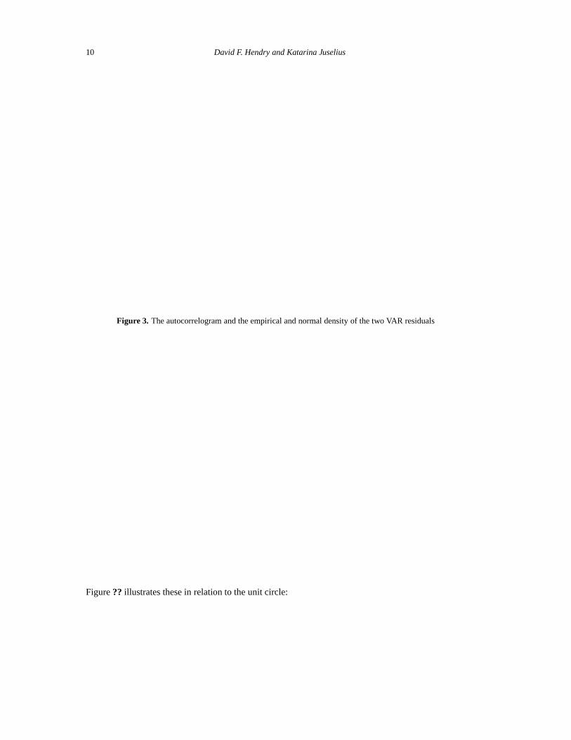
In Figure 3, the autocorrelograms and the empirical densities (with the normal density) are reportedfor the two VAR residuals. There should be no significant autocorrelation, if the truncation after thesecond lag is appropriate. Since all the autocorrelation coefficients are very small, this seems to be thecase. Furthermore, the empirical density should not deviate too much from the normal density; and theresiduals should be homoscedastic, so have similar variances over time. The empirical densities seemto have longer tails (excess kurtosis) than the normal density, and the Kuwait war outlier sticks out,confirming our previous finding of non-normality.
3.4. Stability and unit-root properties
Up to this point, we have discussed (and estimated) the VAR model as if it were stationary, i.e., withoutconsidering unit roots.3 The dynamic stability of the process in (4) can be investigated by calculatingthe roots of: (
Ip − Π1L− Π2L2)xt = Π(L)xt,
3One can always estimate the unrestricted VAR with OLS, but if there are unit roots in the data, some inferences are nolonger standard, as discussed in Hendry and Juselius (2000).

Explaining Cointegration Analysis: Part II 9
1990 1995
.5
.75
1 Price 1
1990 1995
.5
.75
Price 2
1990 1995
-.1
0
.1
.2Diff p1
1990 1995
-.1
0
.1Diff p2
1990 1995
0
.1
.2 Residual 1
1990 1995
0
.1 Residual 2
Figure 2. Graphs of gasoline prices 1 and 2 in levels and differences, with residuals from a VAR(2) and 99%confidence bands
whereLixt = xt−i. Define the characteristic polynomial:
Π(z) =(Ip − Π1z − Π2z
2).
The roots of|Π (z)| = 0 contain all necessary information about the stability of the process and,therefore, whether it is stationary or non-stationary. In econometrics, it is more usual to discuss stabilityin terms of the companion matrix of the system, obtained by stacking the variables such that a first-order system results. Ignoring deterministic terms, we have:(
xt
xt−1
)=(
Π1 Π2
Ip 0
)(xt−1
xt−2
)+(
εt
0
), (6)
where the first block is the original system, and the second merely an identity forxt−1. Now, sta-bility depends on the eigenvalues of the coefficient matrix in (6), and these are precisely the roots of∣∣Π (z−1
)∣∣ = 0 (see e.g., Banerjee, Dolado, Galbraith, and Hendry (1993)). For ap-dimensional VARwith 2 lags, there are2p eigenvalues. The following results apply:
(a) if all the eigenvalues of the companion matrix are inside the unit circle, thenxt is stationary;(b) if all the eigenvalues are inside or on the unit circle, thenxt is non-stationary;(c) if any of the eigenvalues are outside the unit circle, thenxt is explosive.
For the bivariate gasoline-price VAR(2) model, we have2 × 2 = 4 roots, the moduli of which are:
0.93, 0.72, 0.72, 0.56.
10 David F. Hendry and Katarina Juselius
Figure 3. The autocorrelogram and the empirical and normal density of the two VAR residuals
Figure?? illustrates these in relation to the unit circle:

Explaining Cointegration Analysis: Part II 11
The roots of the characteristic polynomial for the VAR(2) model.
We note that the system is stable (no explosive roots), that there is one near-unit root, suggestingthe presence of a stochastic trend, as well as a pair of complex roots (whether a pair of roots is realor complex can depend on the third or smaller digits of the estimated coefficients, so is not usually afundamental property of such a figure). Since there is only one root close to unity for the two variables,the series seem non-stationary and possibly cointegrated.
When there are unit roots in the model, it is convenient to reformulate the VAR into an equilibrium-correction model (EqCM). The next section discusses different ways of formulating such models.
4. Different representations of the VAR
The purpose of this section is to demonstrate that the unrestricted VAR can be given different para-metrizations without imposing any binding restrictions on the parameters of the model (i.e., withoutchanging the value of the likelihood function). At this stage, we do not need to specify the order ofintegration ofxt: as long as the parameters(π,Π1,Π2,Ωε) are unrestricted, OLS can be used toestimate them, as discussed in the previous section. Thus, any of the four parameterizations below,namely (4), (7), (8), or (9) can be used to obtain the first unrestricted estimates of the VAR. Althoughthe parameters differ in the four representations, each of them explains exactly as much of the variationin xt.

12 David F. Hendry and Katarina Juselius
The first reformulation of (4) is into the following equilibrium-correction form:
∆xt = Φ1∆xt−1 − Πxt−1 + π + εt, (7)
whereεt ∼ INp[0,Ωε], with the lagged levels matrixΠ = Ip −Π1−Π2 andΦ1 = −Π2.4 In (7), thelagged levels matrix,Π, has been placed at timet− 1, but could be chosen at any feasible lag withoutchanging the likelihood. For example, placing theΠ matrix at lag2 yields the next parameterization:
∆xt = Φ∗1∆xt−1 − Πxt−2 + π + εt (8)
whereΦ∗1 = (Π1 − Ip) ,with an unchangedΠ matrix.5 In a sense, (7) is more appropriate if one wants
to discriminate between the short-run adjustment effects to the long-run relations (in levels), and theeffects of changes in the lagged differences (the transitory effects). The estimated coefficients and theirp-values can vary considerably between the two formulations (7) and (8), despite their being identicalin terms of explanatory power, and likelihood (note that they have identical errorsεt). Often, manymore significant coefficients are obtained with (8) than with (7), illustrating the increased difficultyof interpreting coefficients in dynamic models relative to static regression models: many significantcoefficients need not imply high explanatory power, but could result from the parameterization of themodel.
The final convenient reformulation of the VAR model is into second-order differences (accelerationrates), changes, and levels:
∆2xt = Φ∆xt−1 − Πxt−1 + π + εt (9)
whereΦ = Φ1−Ip = −Ip−Π2, andΠ remains as before. This formulation is most convenient whenxt containsI(2) variables, but from an economic point of view it also provides a natural decompositionof economic data which cover periods of rapid change, when acceleration rates (in addition to growthrates) become relevant, and more stable periods, when acceleration rates are zero, but growth rates stillmatter. It also clarifies that the ‘ultimate’ variable to be explained is∆2xt, which is often treated as a‘surprise’, but as (9) demonstrates, can be explained by the determinants of the model. Indeed, it canbe seen that treating∆2xt purely as a ‘surprise’ imposesΦ = 0 andΠ = 0, and makes the differencesbehave as random walks.
Although the above reformulations are equivalent in terms of explanatory power, and can be es-timated by OLS without considering the order of integration, inferences on some the parameters willnot be standard unlessxt ∼ I(0). For example, whenxt is non-stationary, the joint significance ofthe estimated coefficients cannot be based on standardF-tests (see Hendry and Juselius (2000) for adiscussion in the context of single-equation models). We will now turn to the issue of non-stationarityin the VAR model.
5. Cointegration in the VAR
We first note that the general condition forxt ∼ I(0) is thatΠ has full rank, so is non-singular. Inthis case,|Π (1)| = |Π| 6= 0, which corresponds to condition (a) in Section 3.4 that all the eigenvaluesshould lie within the unit circle. Stationarity can be seen as follows: stationary variables cannot grow
4In the general VAR(k) model,Φ matrices cumulate the longer lag coefficients of the levels representation.5In the general VAR(k), Φ∗ matrices cumulate the earlier lag coefficients.

Explaining Cointegration Analysis: Part II 13
systematically over time (that would violate the constant-mean requirement), so ifxt ∼ I(0) in (7),thenE[∆xt] = 0. Taking expectations yields:
−ΠE [xt−1] + π = 0 (10)
so whenΠ has full rank,E [xt] = Π−1π. Thus, the levels of stationary variables have a uniqueequilibrium mean – this is precisely why stationarity is so unreasonable for economic variables whichare usually evolving! WhenΠ is not full rank (i.e., whenxt exhibitsI(1) behavior), (10) leaves some ofthe levels indeterminate. At the other extreme, whereΠ = 0, the VAR becomes one in the differences∆xt, and these are stationary ifΦ1 − Ip has full rank, in which casext ∼ I(1). Notice thatΦ1 = Ip
whenΠ = 0 makes∆xt a vector of random walks, soxt ∼ I(2).Section 5.1 presents the conditions for cointegration in theI(1) model as restrictions on theΠ
matrix and Section 5.2 discusses the properties of the vector process when the data areI(1) and coin-tegrated, based on the moving-average representation.
5.1. Determining cointegration in the VAR model
As discussed in Section 3.4, when some of the roots of the system (4) are on the unit circle (case (b)),the vector processxt is non-stationary. However, some linear combinations, denotedβ′xt, might bestationary even though the variables themselves are non-stationary. Then the variables are cointegratedfrom I(1), down one step toI(0), which Engle and Granger (1987) expressed as beingCI(1, 1). Thereare two general conditions forxt ∼ I(1), which we now discuss.
The first condition, needed to ensure that the data are notI(0), is thatΠ has reduced rankr < p, socan be written as:
Π = −αβ′ (11)
whereα andβ arep × r matrices, both of rankr. Substituting (11) into (9) delivers the cointegratedVAR model:
∆2xt = Φ∆xt−1 + α(β′xt−1
)+ π + εt. (12)
An important feature of ‘reduced rank’ matrices likeα andβ is that they have orthogonal complements,which we denote byα⊥ andβ⊥: i.e., α⊥ andβ⊥ arep × (p− r) matrices orthogonal toα andβ(soα′
⊥α = 0 andβ′⊥β = 0), where thep × p matrices(α α⊥) and(β β⊥) both have full rankp.
These orthogonal matrices play a crucial role in understanding the relationship between cointegrationand ‘common trends’ as we explain below (a simple algorithm for constructingα⊥ andβ⊥ from αandβ is given in Hendry and Doornik (1996)). Note that multiplying (12) byα′
⊥ will eliminate thecointegrating relations sinceα′
⊥α = 0.The second condition, which is needed to ensure that the data are notI(2), is somewhat more
technical, and requires that a transformation ofΦ in (12) must be of full rank.6 Here, we will disregardtheI(2) problem and only discuss the case when the footnoted condition is satisfied.
If r = p, thenxt is stationary, so standard inference (based ont, F, andχ2) applies. Ifr = 0,then∆xt is stationary, but it is not possible to obtain stationary relations between the levels of the
6Specifically:α′
⊥Φβ⊥ = ζη′ (13)
whereζ andη are(p − r) × s matrices fors = p − r, which is the number of ‘common stochastic trends’ of first order whenxt ∼ I(1). Thus, (13) must have full rank (s = p − r) for xt ∼ I(1). If s < p − r, then the model containsp − r − ssecond-order stochastic trends, andxt ∼ I(2).

14 David F. Hendry and Katarina Juselius
variables by linear combinations. Such variables do not have any cointegration relations, and hence,cannot move together in the long run. In this case, each of (7)–(9) becomes a VAR model in differencesbut, since∆xt ∼ I(0), standard inference still applies. Ifp > r > 0, thenxt ∼ I(1) and there existr directions in which the process can be made stationary by linear combinations,β′xt. These are thecointegrating relations, exemplified in (2) above by the two price differentials.
5.2. The VAR model in moving-average form
When the characteristic polynomialΠ(z) = Ip − Π1z − Π2z2 contains a unit root, the determinant
|Π(z)| = 0 for z = 1, soΠ(z) cannot be inverted to expressxt as a moving average of current andpastεt. Instead, we must decompose the characteristic polynomial into a unit-root part and a stationaryinvertible part, written as the product:
Π(z) = (1 − z)Π∗(z),
whereΠ∗(z) has no unit roots, and is invertible. The VAR model can now be written as:
(1 − L)xt = ∆xt = [Π∗(L)]−1 εt. (14)
Thus,∆xt is a moving average of current and pastεt. To see the nature of that relation, expand[Π∗(L)]−1 as a power series inL:
[Π∗(L)]−1 = C0 + C1L+ C2L2 + . . . = C(L) (say).
In turn, expressC(L) as:C (L) = C + C∗(L)(1 − L),
soC(1) = C asC∗(1)(1 − 1) = 0. We can now rewrite (14) as:
∆xt = [C + C∗(L)(1 − L)] εt.
By integration (dividing by the difference operator,(1 − L)):
xt = C(
εt
1 − L
)+ C∗(L)εt + x0,
for some initial condition denotedx0, which we set to zero to expressxt as:
xt = Ct∑
i=1
εi + C∗(L)εt. (15)
In (15),xt is decomposed into a stochastic trend,C∑t
i=1 εi, and a stationary stochastic component,et = C∗(L)εt.7 There are (p− r) linear combinations between the cumulated residuals,α′
⊥∑t
i=1 εi
7It can be shown that:C = β⊥(α′
⊥Φβ⊥)−1α′⊥, (16)
so theC matrix is directly related to (13), and can be calculated from estimates ofα, β, andΦ: see e.g., Johansen (1992a).LettingB = β⊥(α′
⊥Φβ⊥)−1, thenC = Bα′⊥, so the common stochastic trends have a reduced-rank representation similar
to the stationary cointegration relations.

Explaining Cointegration Analysis: Part II 15
which define the common stochastic trends that affect the variablesxt with weightsB, whereC =Bα′
⊥. In this sense, there exists a beautiful duality between cointegration and common trends. Thefollowing example illustrates.
Assume that there exists one common trend between the two gasoline price series, and hence onecointegration relation as reported in Hendry and Juselius (2000). Then,r = 1 andp − r = 1, and wecan write the moving-average (common-trends) representation as:(
p1,t
p2,t
)=(b11b21
)( t∑i=1
ui
)+(δ1δ2
)t+
(e1,t
e2,t
), (17)
whereB′ = (b11, b21) are the weights of the estimated common trend given byui = α′⊥εi, and
δ1, δ2 are the coefficients of linear deterministic trends inp1,t, p2,t, respectively. Hendry and Juselius(2000) showed that (p1,t − p2,t) ∼ I(0), i.e., that the two prices were cointegrated withβ′ = (1,−1).Furthermore, the assumption behind the single-equation model in Hendry and Juselius (2000) was thatα′ = (∗, 0).These estimates ofβ andα correspond toB′ = (1, 1) andα′
⊥ = (0, 1) in (17). Weexpress this outcome as: cumulated shocks top2,t give an estimate of the common stochastic trend inthis small system. Both prices are similarly affected by the stochastic trend, so that in:
(p1,t − p2,t) = (b11 − b21)t∑
i=1
ui + (δ1 − δ2)t+ (e1,t − e2,t) (18)
we have(b11 − b21) = 0, and the linear relation (p1,t − p2,t) has no stochastic trend left, therebydefining a cointegration relation.
Note that (17) also allows for a deterministic linear trendt in xt. If, in addition,δ1 = δ2, then boththe stochastic and the linear trend will cancel in the linear relation (p1,t − p2,t) in (18). If δ1 6= δ2,then we need to allow for a linear trend in the cointegration relation, such that (p1,t − p2,t − d1t)contains neither stochastic nor deterministic trends. In this case, we say that the price differential istrend stationary, and that there is a trend in the cointegration space. We have reached the stage wherewe need a more complete discussion of the key role played by deterministic terms in cointegratedmodels.
6. Deterministic components in a cointegrated VAR
A characteristic feature of the equilibrium-correction formulation (12) is the inclusion of both differ-ences and levels in the same model, allowing us to investigate both short-run and long-run effects inthe data. As discussed in Hendry and Juselius (2000), however, the interpretation of the coefficientsin terms of dynamic effects is difficult. This is also true for the trend and the constant term,as well asother deterministic terms like dummy variables. The following treatment starts from the discussion ofthe dual role of the constant term and the trend in the dynamic regression model in Hendry and Juselius(2000), and extends the results to the cointegrated VAR model.
When two (or more) variables share the same stochastic and deterministic trends, it is possibleto find a linear combination that cancels both the trends. The resulting cointegration relation is nottrending, even if the variables by themselves are. In the cointegrated VAR model, this case can beaccounted for by including a trend in the cointegration space. In other cases, a linear combination ofvariables removes the stochastic trend(s), but not the deterministic trend, so we again need to allow for
16 David F. Hendry and Katarina Juselius
a linear trend in the cointegration space. Similar arguments can be used for an intervention dummy:the intervention might have influenced several variables similarly, such that the intervention effectcancels in a linear combination of them, and no dummy is needed. Alternatively, if an interventiononly affects a subset of the variables (or several, but asymmetrically), the effect will not disappear inthe cointegration relation, so we need to include an intervention dummy.
These are only a few examples showing that the role of the deterministic and stochastic componentsin the cointegrated VAR is quite complicated. However, it is important to understand their role inthe model, partly because one can obtain misleading (biased) parameter estimates if the deterministiccomponents are incorrectly formulated, partly because the asymptotic distributions of the cointegrationtests are not invariant to the specifications of these components. Furthermore, the properties of theresulting formulation may prove undesirable for (say) forecasting, by inadvertently retaining unwantedcomponents – such as quadratic trends, as illustrated by Case 1 below. In general, parameter inference,policy simulations, and forecasting are much more sensitive to the specification of the deterministicthan the stochastic components of the VAR model. Doornik, Hendry, and Nielsen (1998) provide acomprehensive discussion.
6.1. Intercepts in cointegration relations and growth rates
Another important aspect is to decompose the intercept,π, into components that induce growth inthe system, and those that capture the means of the cointegration relations.8 Reconsider the VARrepresentation (7):
∆xt = Φ1∆xt−1 + α(β′xt−1
)+ π + εt (19)
where∆xt ∼ I(0) andεt ∼ I(0). To ‘balance’ (19),β′xt−1 must beI(0) also. Since ther cointeg-ration relationsβ′xt−1 are stationary, each of them has a constant mean. Similarly, ∆xt is stationarywith a constant mean, which we denote byE[∆xt] = γ, describing a (p × 1) vector of growth rates.This was illustrated in (17) by allowing for linear trends in the two prices with slope coefficientsδ1andδ2. Furthermore, letE
[β′xt−1
]= µ describe a(r × 1) vector of intercepts in the cointegrating
relations. We now take expectations in (19):
(Ip − Φ1)γ = αE[β′xt−1
]+ π = αµ + π.
Consequently,π = (Ip − Φ1) γ − αµ. Note that the constant termπ in the VAR model does indeedconsist of two components: one related to the linear growth rates in the data, and the other relatedto the mean values of the cointegrating relations (i.e., the intercepts in the long-run relations). Thisdecomposition is similar to the simpler single-equation case discussed in Hendry and Juselius (2000).When the cointegration relations are trend free as in (19):
β′E [∆xt] = E[∆β′xt
]= β′γ = 0,
so we can express (19) in mean-deviation form as:
(∆xt − γ) = Φ1 (∆xt−1 − γ) + α(β′xt−1 − µ
)+ εt. (20)
There are two forms of equilibrium correction in (20): that of the growth∆xt in the system to itsmeanγ; and of the cointegrating vectorsβ′xt−1 to their meanµ. The two mean values,γ and
8One of the reasons we assume all the variables are in logs is to avoid the growth rates depending on the levels of thevariables.

Explaining Cointegration Analysis: Part II 17
µ, play an important role in the cointegrated VAR model, and it is important to ascertain whetherthey are significantly different from zero or not at the outset of the empirical analysis. In the nextsubsection, we will present five baseline cases describing how the trend and the intercept can enter theVAR specification.
6.2. Five cases for trends and intercepts
The basic ideas are illustrated using thep-dimensional cointegrated VAR with a constant and a lineartrend, but to simplify notations we assume that only one lag is needed, soΦ1 = 0. As before,εt ∼INp [0,Ωε]:
∆xt = αβ′xt−1 + π + δt+ εt. (21)
Without loss of generality, the two(p × 1) vectorsπ andδ can each be decomposed into two newvectors, of which one is related to the mean value of the cointegrating relations,β′xt−1 (case (3) insection 2 of Hendry and Juselius (2000)), and the other to growth rates in∆xt:
π = αµ + γ0
δ = αρ + τ(22)
Substituting (22) into (21) yields:
∆xt = αβ′xt−1 + αµ + γ + αρt+ τ t+ εt, (23)
so, collecting terms in (23):
∆xt = α(β′ : µ : ρ
) xt−1
1t
+ (γ + τ t) + εt. (24)
Thus, we can rewrite (21) as:
∆xt = α
βµ′
ρ′
′
x∗t−1 + (γ + τ t) + εt, (25)
wherex∗t−1 = (x′
t−1, 1, t)′. We can always chooseµ andρ such that the equilibrium error(β∗)′ x∗t =
vt has mean zero (whereβ∗ =(β′,µ,ρ
)′), so the trend component in (25) can be interpreted from
the equation:E [∆xt] = γ + τ t. (26)
Thus,γ 6= 0 corresponds to constant growth in the variablesxt (case 1 in section 2 of Hendry andJuselius (2000)), whereasτ 6= 0 corresponds to linear trends in growth, and so quadratic trends in thevariables. Hence, the constant term and the deterministic linear trend play a dual role in the cointegratedmodel: in theα directions they describe a linear trend and an intercept in the steady-state relations; inthe remaining directions, they describe quadratic and linear trends in the data. To correctly interpretthe model, one has to understand the distinction between the part of the deterministic component that‘belongs’ to the cointegration relations, and the part that ‘belongs’ to the differences.
In empirical work, usually one has some idea whether there are linear deterministic trends in some(or all) of the variables. It might, however, be more difficult to know if they cancel in the cointegrating

18 David F. Hendry and Katarina Juselius
relations or not. Luckily, we do not need to know beforehand, because the econometric analysis canbe used to find out. As discussed below, all these cases can be expressed as linear restrictions onthe deterministic components of the VAR model and, hence, can be tested. We now discuss five ofthe most frequently used models arising from restricting the deterministic components in (21): seeJohansen (1994).
Case 1. No restrictions onπ andδ, so the trend and intercept areunrestrictedin the VAR model. Withunrestricted parameters,π, δ, the model is consistent with linear trends in the differenced series∆xt as shown in (26) and, thus, quadratic trends inxt. Although quadratic trends may some-times improve the fit within the sample, forecasting outside the sample is likely to produceimplausible results. Be careful with this option: it is preferable to find out what induced theapparent quadratic growth and, if possible, increase the information set of the model. Moreover,as shown in Doornik, Hendry, and Nielsen (1998), estimation and inference can be unreliable.
Case 2. τ = 0, butγ, µ, ρ remain unrestricted, so the trend isrestrictedto lie in the cointegration space,but the constant is unrestricted in the model. Thus,τ being zero in (25) still allows linear, butprecludes quadratic, trends in the data. As illustrated in the previous section,E[∆xt] = γ 6= 0implies linear deterministic trends in the levelxt.When, in addition,ρ 6= 0, these linear trends inthe variables do not cancel in the cointegrating relations, so the model contains ‘trend-stationary’relations which can either describe a single trend-stationary variable, (x1,t − b1t) ∼ I(0), or anequilibrium relation (β′
1xt − b2t) ∼ I(0). Therefore, the hypothesis that a variable is trend-stationary can be tested in this model.
Case 3. δ = 0, so there are no linear trends in (21). Since the constant termπ is unrestricted, there arestill linear trends in the data, but no deterministic trends in any cointegration relations. Also,E[∆xt] = γ 6= 0, is consistent with linear deterministic trends in the variables but, sinceρ = 0,these trends cancel in the cointegrating relations. It appears from (24) thatπ 6= 0 accounts forboth linear trends in the DGP and a non-zero intercept in the cointegration relations.
Case 4. δ = 0, γ = 0, butµ 6= 0,so the constant term isrestrictedto lie in the cointegration space in(25). In this case, there are no linear deterministic trends in the data, consistent withE[∆xt] = 0.The only deterministic components in the model are the intercepts in any cointegrating relations,implying that some equilibrium means are different from zero.
Case 5. δ = 0 andπ = 0, so the model excludes all deterministic components in the data, with bothE[∆xt] = 0 andE[β′xt] = 0, implying no growth and zero intercepts in every cointegrating re-lation. Since an intercept is generally needed to account for the initial level of measurements,x0,only in the exceptional case when the measurements start from zero, or when the measurementscancel in the cointegrating relations, can the restrictionπ = 0 be justified.
Turning to our empirical example, Table 1 showed thatE[∆pi,t] = 0 could not be rejected. Hence,there is no evidence of linear deterministic trends in the gasoline prices, at least not over the sampleperiod. The graphs in Figure 1 support this conclusion. We conclude that the cointegrated VAR modelshould be formulated according to case 4 here, with the constant term restricted to the cointegrationspace, and no deterministic trend terms.
7. The likelihood-based procedure
So far, we have discussed the formulation of the VAR model in terms of well-specified stochastic anddeterministic properties. All this can be done before addressing the unit-root problem. As in Hendry

Explaining Cointegration Analysis: Part II 19
and Juselius (2000), we will now assume that some of the roots of the characteristic polynomial are onthe unit circle. This means thatxt ∼ I(1), and we consider the cointegrated VAR(2) model (7) whereΠ = −αβ′ with a constant, a linear trend and a vector of dummy variablesdt included:
∆xt = Φ1∆xt−1 + αβ′xt−1 + π + δt+ Ψdt + εt. (27)
Since∆xt ∼ I(0) andεt ∼ I(0), all stochastic components in (27) are stationary by definition exceptfor β′xt−1. For (27) to be internally consistent, given thatxt ∼ I(1), β cannot be a full-rankp × pmatrix (because then something stationary would be equal to something non-stationary). The onlypossible solution is thatβ is a reduced rank (p× r) matrix withr < p, sor linear combinations cancelstochastic trends as shown in section 5. Below, we will only discuss the broad ideas of the maximumlikelihood estimation procedure, and will not go through the derivations of the results. The interestedreader is referred to Johansen (1988, Johansen (1995) and Banerjee, Dolado, Galbraith, and Hendry(1993),inter alia, for details.
The derivation of the maximum likelihood estimator (MLE) is done via the ‘concentrated likeli-hood’ of the VAR model. Since the latter is crucial for understanding both the statistical and economicproperties of the VAR, we will demonstrate how it is defined. We use the following shorthand notation:
z0,t = ∆xt
z1,t = xt−1
z2,t = (∆xt−1,1, t,dt) .
(additional lagged differences are easily included inz2,t). Rewrite (27) as:
z0,t = αβ′z1,t−1 + Θz2,t + εt,
whereΘ = (Φ1,π, δ,Ψ). By concentrating out the short-run dynamic adjustment effects,Θz2,t,we are able to obtain a ‘simpler’ model. This is done by first defining the following auxiliary OLSregressions:
z0,t = D′1z2,t + ∆xt
z1,t = D′2z2,t + xt−1,
where∆xt = z0,t − M02M−122 z2,t and xt−1 = z1,t − M12M−1
22 z2,t are the OLS residuals, andMij =
∑t(zi,tz′j,t)/T is a product-moment matrix, so thatD′
1 = M02M−122 andD′
2 = M12M−122 .
The concentrated model can now be written as:
∆xt = αβ′xt−1 + ut, (28)
so we have transformed the original VAR containing short-run adjustments and intervention effectsinto the ‘baby model’ form, in which the adjustments are exclusively towards the long-run steady-staterelations.
The MLE is close to limited-information maximum likelihood (LIML: see Hendry (1976) for aconsolidation) in that the key issue is to handle a reduced-rank problem, which essentially amounts tosolving an eigenvalue problem. In practice, the estimators are derived in two steps. First, to derivean estimator ofα, assume thatβ is known: thenβ′xt−1 becomes a known variable in (28), soαcan be estimated by OLS. Next, insert thatα = α(β) in the expression for the concentrated likelihoodfunction, which becomes a function ofβ alone, and no longer depends onα. To find the value ofβ thatmaximizes this likelihood function is a non-linear problem, but one that can be solved by reduced-rankregression (see Johansen (1988)). The solution deliversp eigenvaluesλi where0 ≤ λi ≤ 1:
λ′= (λ1, λ2, . . . , λp) ,
20 David F. Hendry and Katarina Juselius
which are ordered such thatλ1 ≥ λ2 ≥ · · · ≥ λp. The estimate ofβ for r cointegrating vectors isgiven by thep × r matrix of eigenvectors corresponding to the largestr eigenvalues (the selection ofr is discussed in Section 8). Given the MLEβ of β, calculateα = α(β). The estimates of the twoeigenvectors, and the correspondingα weights for the empirical example are reported in Table 3.
Eachλi can be interpreted as the squared canonical correlation between linear combinations of thelevels,β′
ixt−1, and a linear combination of the differences,ϕ′i∆xt . In this sense, the magnitude ofλi
is an indication of how strongly the linear combinationβ′ixt−1 is correlated with the stationary part of
the processϕ′i∆xt. If λi ≈ 0, the linear combinationβ′
ixt−1 is not at all correlated with the stationarypart of the process, and hence is non-stationary.
In the situation where bothα andβ are unrestricted (beyond normalizations), standard errors can-not be obtained, but the imposition of rank and other identifying restrictions usually allows appropriatestandard errors to be obtained forα andβ.
8. Testing cointegration rank
Given that the unrestricted VAR model has been found to satisfactorily describe the data (is a congruentrepresentation), one can start the simplification search, which means imposing valid restrictions onthe model such as a reduced-rank restriction, restrictions on the long-run parametersβ, and finallyrestrictions on the short-run adjustment parametersα andΦ. The first, and most crucial, step is todiscriminate empirically between zero and non-zero eigenvalues when allowing for sample variation,and then impose an appropriate cointegration rank restrictionr on theΠ matrix. Note that:
• if we underestimater, then empirically-relevant equilibrium-correction mechanisms (EqCMs)will be omitted;
• whereas if we overestimater, the distributions of some statistics will be non-standard, so thatincorrect inferences may result from using conventional critical test values (based ont, F, χ2);
• forecasts will be less accurate due to incorrectly retainingI(1) components, which will increaseforecast variances.
A test for r cointegrating vectors can be based on the maximum likelihood approach proposedby Johansen (1988). The statistical problem is to derive a test procedure to discriminate betweentheλi, i = 1, . . . , r, which are large enough to correspond to stationaryβ′
ixt−1, and thoseλi, i =r + 1, . . . , p, which are small enough to correspond to non-stationary eigenvectors. The rankr isdetermined by a likelihood-ratio test procedure between the two hypotheses:
Hp: rank= p, i.e., full rank, soxt is stationary;Hr: rank= r < p, i.e.,r cointegration relations.
The test is:
LR(Hr | Hp) = −T ln [(1 − λr+1) · · · (1 − λp)] = −Tp∑
i=r+1
ln(1 − λi).
If λr+1 = · · · = λp = 0, the test statistic should be small (close to zero), which delivers the criticalvalue under the null. The test is based on non-standard asymptotic distributions that have been sim-ulated for the five cases discussed in section 6. There is an additional problem, in thatHr may becorrectly accepted whenλr = 0, or evenλr−1 = 0. Therefore, ifHr is accepted, we conclude that
Explaining Cointegration Analysis: Part II 21
there are at leastp − r unit roots, i.e.,p − r ‘common trends’ in the process (but there can be more)corresponding to at mostr stationary relations.
However, ifLR(Hr−1|Hp) is calculated, the test statistic includesln(1 − λr), which will not beclose to zero, so an outcome in excess of the critical value should be obtained, correctly rejecting thefalse null of fewer thatr cointegration relations.
As discussed above, the asymptotic distributions depend on whether there is a constant and/or atrend; and whether these are unrestricted or not in the model. However other deterministic compon-ents, such as intervention dummies, are also likely to influence the shape of the test distributions. Inparticular, care should be taken when a deterministic component generates trending behavior in thelevels of the data such as an unrestricted shift dummy (· · · ,0,0,0,1,1,1,· · ·): an explanation of the pro-cedure is provided in Johansen, Nielsen, and Mosconi (2000), and Juselius (2000): Doornik, Hendry,and Nielsen (1998) also consider the estimation and inference problems resulting from including dum-mies.
Because the asymptotic distributions for the rank test depend on the deterministic componentsin the model and on whether these are restricted or unrestricted, the rank and the specification of thedeterministic components have to be determined jointly. Nielsen and Rahbek (1998) have demonstratedthat a test procedure based on a model formulation that allows a deterministic component, for examplea deterministic trendt, to be restricted to the cointegration relations and the differenced component,∆t = 1, to be unrestricted in the model induces similarity in the test procedure (i.e., the critical valuesdo not depend on the parameter values, so can be tabulated). This is because when there are lineartrends in the data, i.e.E[∆xt] 6= 0, they can enter the model through the constant term,γ 6= 0 in (26)or through the cointegration relations,ρ 6= 0 in (25). Hence, given linear trends in the data, case 2 isthe most general case. When the rank has been determined, it is always possible to test the hypothesisρ = 0, as a linear restriction on the cointegrating relations.
If, on the other hand,E[∆xt] = 0, so there are no linear trends in the data, then the baseline modelhas the constant term restricted to the cointegration space, which is case 4 above. Therefore, based onthe similarity argument, the rank should be based on either case 4 (trends in the data) or case 2 (notrends in the data). Nevertheless, if there is strong prior information that there are trends in the data,but they do not appear in the cointegration relations, then case 3 is the appropriate choice.
9. Empirical model specification
The rank test is defined for a correctly specified model. Prior to the determination of the cointegrationrank we should make sure that the empirical model is well-behaved. In Section 9.1, we choose thetrend and constant in the baseline model, and account for the extraordinary events in the sample period;whereas in Section 9.2, we discuss the difficult choice of cointegration rank.
9.1. Model specification
For the gasoline example, we found in Table 1 thatE[∆xt] = 0 cannot be rejected. Hence, thereis little evidence of linear deterministic trends in the data, at least not over the sample period, so weshould determine the rank based on a case-4 model. But before testing the rank of theΠ matrix, weneed to account for the effect of the Kuwait war on gasoline prices as discussed in Section 3.2, pluspossibly some of the extraordinary price changes in this period that violate the normality assumption.
22 David F. Hendry and Katarina Juselius
Table 2. The estimates of the short-run effects
Φ The Kuwait war effects Ωε
∆p1,t−1 ∆p2,t−1 ∆Ds90.31t ∆Ds90.31t−1 ε1,t ε2,t
∆p1,t 0.52(11.3)
0.14(2.3)
0.18(7.8)
−0.09(4.0)
ε1,t 1.0
∆p2,t 0.05(1.3)
0.53(12.0)
0.11(5.8)
−0.02(1.2)
ε2,t 0.66 1.0
The estimates of the extraordinary price changes (|εi,t| > 3.3)
Di89.13 Di89.39 Di89.51 Di90.49 Di9103 Di93.43 Dti98.11
∆p1,t 0.08(3.6)
−0.08(3.9)
0.09(4.1)
−0.08(3.5)
−0.09(3.9)
−0.05(2.5)
−0.08(4.7)
∆p2,t 0.07(3.7)
−0.04(2.0)
0.05(2.9)
−0.07(3.6)
−0.08(4.2)
−0.08(4.6)
−0.03(2.5)
The question is now which kind of intervention dummies should be used to describe these ex-traordinary events. Juselius and Johansen (2000), show that a shift in the level of the variables corres-ponds to a permanent impulse blip in the differences, and an impulse effect in the levels correspondsto a transitory blip in the differences. The Kuwait war could have caused either a permanent or a trans-itory shift in the level of gasoline prices. In the latter case, we would see an initial rise in the gasolineprices in 1990:31 followed later on by a return to the previous price level. Based on the graphs in Fig-ure 1, the differences show a large positive spike followed by another more moderately sized negativespike a few weeks later. This suggests that the initial increase in prices was partly permanent, partlytransitory. To account for this extraordinary event on the price levels, the model includes a step dummy,Ds90.31t being zero up tot = 1990:31 and unity after that,restrictedto lie in the cointegration space(if significant, then the permanent price increase in crude oil as a result of the war had a different effecton gasoline prices in the two locations). To account for the effect on the price changes, we also needto include current and lagged values of the impulse dummyDi90.31t, defined below, asunrestrictedin the model. Table 2 shows that the estimated direct price effect at the outbreak of the Kuwait warwas an increase of 18% in location 1 and 11% in location 2, followed by a drop in the price by 9% inlocation 1 and 2% in location 2. Hence, the permanent effect of the war seemed to be approximately9% in both locations. Altogether, the immediate price reaction in location 1 seemed to be stronger thanin location 2.
Based on the criterion|εi,t| > 3.3, we detected seven additional ‘outlier’ observations, accountedfor by dummy variables defined as follows: the impulse dummyDixx.yyt is unity for t = 19xx:yy,and zero otherwise; the transitory impulse dummyDtixx.yyt is unity for t = 19xx:yy, −1 for t =19xx:yy+1, and zero otherwise. Table2 reports the estimates of these very large price changes. Again,we note that the price reactions in location 1 seem stronger than in location 2: except for 1993:43,gasoline prices in location 1 change more dramatically than in location 2.
The estimates of theΦ matrix in Table2 demonstrate quite strong autoregressive price behavior: aprice change one week tends to be followed by a similar change but only half the size, next week. Italso appears that a price change byp2,t is followed by a lagged change inp1,t, but not the other wayaround. The estimates of the residual covariance matrixΩε show a large positive correlation betweenprice shocks to the two gasoline prices, which suggests that there may be current, as well as lagged,price effects. This will be further discussed in Section 11.
After having accounted for these extraordinary events, the distributions of the residuals became
Explaining Cointegration Analysis: Part II 23
much closer to a normal distribution than in the first tentatively estimated model. However, the empir-ical model still showed some evidence of excess kurtosis and ARCH (autoregressive conditional hetero-scedasticity, so the squared residuals are serially correlated: see Engle (1982)), as appears from Table3, but neither of these usually causes serious problems for the properties of the estimates (Gonzalo,199*). A plausible explanation for these problems is that the residual variance of the process changesin the middle of the sample, at around 1992:40. We have analyzed the data separately for the splitsample, and the ARCH and excess kurtosis disappear. However, the basic results remained unchangedin the two sub-samples and there is, therefore, no obvious need to report the results separately. Weconclude that the empirical model is reasonably well specified, and turn to the determination of thecointegration rank.
9.2. Rank determination
As already mentioned, a correct choice of the cointegration rank is crucial for the analysis, but inpractice, is far from easy. In many economic applications, the size of the sample is often quite small,and the tabulated asymptotic distributions can be rather poor approximations as has been demonstratedin many papers. See, for instance, Johansen (1999) for analytical results, and (ref.) for Monte Carloor bootstrap results. Another reason for concern is that when using correct small-sample distributionsfor the trace test, the size of the test is correct, but the power can be low, sometimes even of the samemagnitude as the size. In such cases, a 5% test procedure will reject a unit root incorrectly 5% of thetime, but accept a unit root incorrectly 95% of the time!
Thus, unless a unit root is given a structural interpretation (and hence, should be tested rigorously),it is important to make the decision based on as much information as possible, including prior economicinformation, and sensitivity analyses of doubtful cases to find out if important information is lost byleaving out therth + 1 cointegration vector, or if anything is gained by including it.
The following information is often useful when deciding on the choice of cointegration rank:
1. the trace test for cointegration rank;2. the characteristic roots of the model: if therth + 1 cointegration vector is non-stationary and is
wrongly included in the model, then the largest characteristic root will be close to the unit circle;3. thet-values of theα-coefficients for therth + 1 cointegration vector; if these are all small, say
less than 3.0, then one would not gain greatly by including that vector as a cointegrating relationin the model;
4. the recursive graphs of the trace statistic forr = 1, 2, . . . , p: since the variableTj ln(1−λi), forj = T1, . . . , T, grows linearly over time whenλi 6= 0, the recursively-calculated componentsof the trace statistic should increase linearly for the firstr components, but stay constant for theremainder;
5. the graphs of the cointegrating relations: if the graphs reveal distinctly non-stationary behaviorof a cointegration relation, which is supposedly stationary, one should reconsider the choice ofr,or find out if the model specification is in fact incorrect, for example, if the data areI(2) insteadof I(1);
6. the economic interpretability of the results.
We will consider all the above pieces of information in turn:The trace test (item 1) in the bivariate gasoline price case, should be able to discriminate between
the following alternatives: no unit roots, one unit root, or two unit roots. The first case corresponds to
24 David F. Hendry and Katarina Juselius
Table 3. Rank and specification tests
Rank determination The two largest roots Misspecification tests
λi Trace Q95 (r = 2) (r = 1) ARCH Norm. R2
0.13 91.1 20.0 0.93 1.00 ∆p1 9.8 17.8 0.54
0.02 14.4 9.1 0.72 0.72 ∆p2 8.3 20.3 0.48
The unrestricted cointegration vectors and their weights
p1 p2 Ds90.31 constant β′1xt β
′2xt
β′1 1.0 −0.97 −0.02 0.02 ∆p1 : α1. −0.15
(7.5)−0.02(2.1)
β′2 −0.25 1.0 0.03 0.41 ∆p2 : α2. −0.02
(1.2)−0.03(3.8)
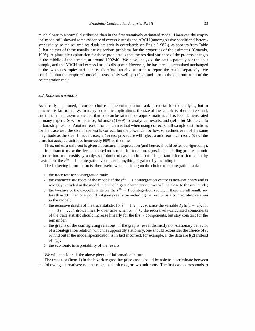
prices being stationary, the second to them beingI(1) with one stationary cointegration relation, andthe last case to them beingI(1) but with no cointegrating relation between them. The two trace teststatistics in Table 3 are larger than their 95% quantiles, so that bothλ1 andλ2 have to be considereddifferent from zero, suggesting that both price series are stationary. As mentioned aboveλi can beinterpreted as a squared canonical correlation coefficient. It appears from the table that bothλ1 andλ2
are small in absolute value, indicating a fairly low correlation with the stationary part, and thatλ1 ismuch larger thanλ2, suggesting that the adjustment to the first cointegration relation is much strongerthan to the second. The graphs of the cointegration vectors (item 5) in Figure 4 indicate that bothare mean-reverting, but the second one much more strongly so. The two largest characteristic roots(item 2) show thatr = 2 implies a fairly large root, 0.93, in the model. The recursive graphs (item4) of Tj ln(1 − λ1j ) andTj ln(1 − λ2j ) in Figure??show that the second component remains almostconstant, whereas the first grows linearly over time. All this suggests that the first cointegrating relationis stationary and that the second is near integrated, but with significant mean reversion. A similar resultwas found in Hendry and Juselius (2000).
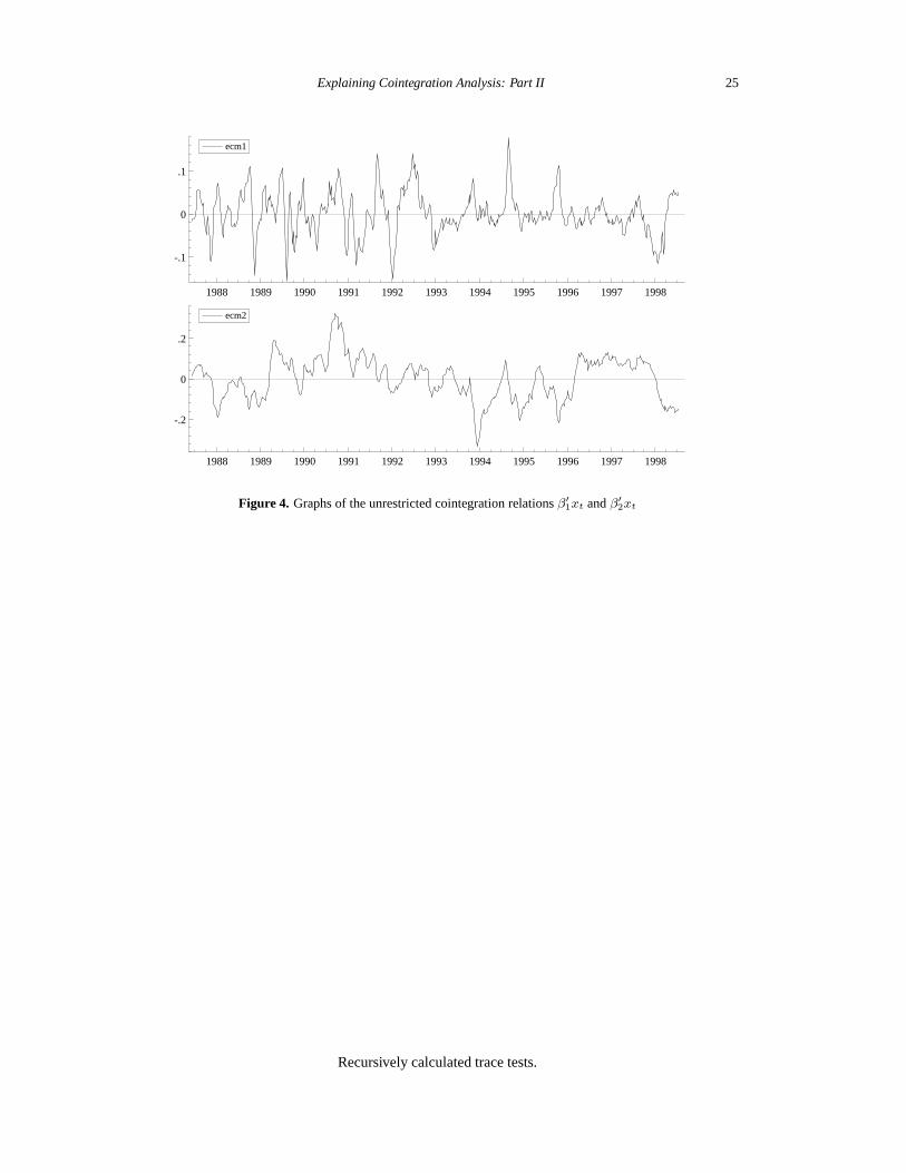
Explaining Cointegration Analysis: Part II 25
1988 1989 1990 1991 1992 1993 1994 1995 1996 1997 1998
-.1
0
.1
ecm1
1988 1989 1990 1991 1992 1993 1994 1995 1996 1997 1998
-.2
0
.2
ecm2
Figure 4. Graphs of the unrestricted cointegration relationsβ′1xt andβ′
2xt
Recursively calculated trace tests.
26 David F. Hendry and Katarina Juselius
Why does the trace test find that the small value ofλ2 = 0.02 is still significantly different fromzero? The simple explanation is that the sample size is very large here, 576 observations. Because thetrace test is calculated asT ln(1−λ), even a small deviation from zero can be found to be significantwhenT is large enough. However, inference is much closer to the so called Dicky–Fuller distributionsthan to standardt-, F-, andχ2-distributions when there is a near unit root in the model. Hence, to makeinference more robust, it is often a good idea to approximate a near unit root by a unit root even whenit is found to be statistically different from one.
Before finally deciding about the rank, we first check the economic interpretability of the secondcointegration relation to see if it contains valuable information for the analysis. It appears from Table3 that the adjustment coefficients to the second relationα21 andα22 (item 3) are very small,α21
is hardly significant in the first gasoline price equation, whereasα22 is more significant in the second
price equation. Nevertheless, the coefficients ofβ′2xt (item 6) indicate that it is essentially a unit vector
describing price 2. This is confirmed by the graphs of the cointegration vectors (item 5) in Figure 4,where the second graph closely resemblesp2,t in Figure 2. Therefore, acceptingr = 2 is equivalentto saying that the gasoline prices are stationary, albeit subject to substantial persistence. As alreadydiscussed in Hendry and Juselius (2000), this might be the case, but choosingr = 2 would leave a nearunit root in the model, and conventional (t-, F-, χ2) inference is likely to be misleading. Moreover,asserting a constant long-run mean for nominal gasoline prices does not seem plausible. Finally, sinceβ′
2xt will not add much valuable information about the co-movements of the two gasoline prices, weconclude that the empirical analysis will not benefit from choosingr = 2. We therefore continue theempirical analysis assumingr = 1.
10. Identification and hypothesis testing
Given the choice of the number of cointegrating relations,r, the Johansen procedure gives the max-imum likelihood estimates of the unrestricted cointegrating relationsβ′xt. Although the unrestrictedβ is uniquely determined based on the chosen normalization, the latter is not necessarily meaningfulfrom an economic point of view. Therefore, an important part of a long-run cointegration analysis isto impose (over-) identifying restrictions onβ to achieve economic interpretability. In section 10.1,we discuss a typology of restrictions onβ and note the problem of calculating the degrees of freedomin the case of over-identifying restrictions. Section 10.2 provides some examples of how to specifyhypotheses in a testable form.
10.1. Restrictions onβ
As an example of just-identifying restrictions, consider the following design matrixQ = (β1) whereβa is a (r × r) non-singular matrix defined byβ′ = (βa,βb). In this case,αβ′ = α(βaβ−1′
a β′) =α(Ir, β) whereIr is the (r × r) unit matrix, andβ = β−1′
a βb is an(r × (p− r)) full-rank matrix.These just-identifying restrictions have transformedβ to the long-run ‘reduced form’. Because just-identifying restrictions do not change the likelihood function, no tests are involved. In general, justidentification can be achieved by imposing one appropriate normalization and(r − 1) restrictions oneachβi. Care is required to ensure that the coefficient which is normalized is non-zero.
The calculation of the degrees of freedom when testing structural hypotheses on the cointegrationrelations is often quite difficult. It is useful from the outset to distinguish between:

Explaining Cointegration Analysis: Part II 27
1. pseudo ‘restrictions’ that can be obtained by linear manipulations, because it is always possibleto imposer − 1 restrictions and one normalization without changing the value of the likelihoodfunction – no testing is involved for such ‘restrictions’;
2. additional testable restrictions on the parameters, which change the value of the likelihood func-tion;in the latter group there are two kinds of testable restrictions:
(a) restrictions that are not identifying, for example: (i) the same restrictions on all cointegrat-ing vectors, (ii) one vector assumed known and the remaining vectors unrestricted.
(b) genuine over-identifying restrictions.
The first step is to examine whether the restrictions satisfy the rank and order condition for identifica-tion: luckily, many available software packages do the checking, and will usually inform the user whenidentification is violated. Also, note that when normalizing aβi vector by diving through by a non-zero elementβij , the correspondingαi vector will by multiplied by the same element, so normalizationdoes not changeΠ = αβ′.
10.2. Hypotheses testing
Hypotheses on the cointegration vectors can be formulated in two alternative ways: either by specifyingthesi free parameters in eachβ vector, or by specifying themi restrictions on each vector. We considereach in turn. First:
β = (H1κ1, ...,Hrκr),
whereβ is (p1 × r), κi are(si × 1) coefficient matrices, andHi are(p1 × si) design matrices wherep1 is the dimension ofx∗
t−1 in (25). In this case, we use the design matrices to determine thesi freeparameters in each cointegration vector.
The other way of formulating restrictions is:
R′1β1 = 0, ...,R′
rβr = 0
whereRi is ap×mi restrictions matrix. Note thatRi = H⊥,i, i.e.,R′iHi = 0.
In some cases, we may want to test restrictions which are not identifying. Such restrictions couldbe the same restriction on all cointegration relations, for example long-run price homogeneity on allvectors. In this case, theHi (orRi) are all identical, and we can formulate the hypothesis asβ = Hκ,whereκ is now ans × r matrix of free parameters. Another possibility is to test a hypothesis on justone of the cointegration vectors. In this case, we formulate the hypothesis asβ = H1κ1,κ2, ...,κr,whereH1 is a (p × s1) matrix, κ1 is (s1 × 1), and the other vectors are unrestricted. All thesehypotheses can be tested by a likelihood-ratio procedure described in detail in Johansen and Juselius(1990, Johansen and Juselius (1992) Johansen. and Juselius (1994).
Our simple empirical example consists of only two gasoline prices, so the number of interestinghypotheses to test is limited. Here, we will only test one hypothesis as an illustration and refer theinterested reader to the many published papers containing a wide variety of testable hypotheses, forexample Juselius ... . Table 3 showed that the unrestricted coefficients of the first cointegration vectorwere almost equal with opposite signs, indicating long-run price homogeneity. This hypothesis can beformulated either asβ = (Hκ) or, equivalently, asR′β = 0, where:
H′ =
1 −1 0 00 0 1 00 0 0 1
, κ =
κ1
κ2
κ3
, andR′ =(
1 1 0 0).
28 David F. Hendry and Katarina Juselius
The first alternative specifies the hypothesis in terms of thes1 = 3 remaining free parameters; thesecond in terms of them1 = 1 imposed restriction. The hypothesis is tested by the LR test proceduredescribed in Johansen and Juselius (1992). The test statistic value was 0.55, distributed asχ2(1), andhence accepted with ap-value of 0.46. The restricted cointegration relation became:
p1 − p2 − 0.02(1.8)
Ds94.34−0.010(0.6)
α11 =−0.14(7.3)
, α12 =−0.01(0.8)
The constant term is not significantly different from zero, but for reasons discussed above in Section6, we prefer to keep it in the cointegration relation. Similarly, the step dummy is only borderlinesignificant (cf. the discussion in Section 9.1), and suggests that the permanent increase in gasolineprices at location 1 might (possibly) have been slightly higher than at location 2. The estimates of theadjustment coefficientsα1i show significant adjustment in the first price, but not in the second. Thissuggests that a price shock leading to an increase in the price differential between the two locationswill initiate an adjustment in the first price, but not in the second: in this sense, the second location isa price leader, i.e., is ‘driving’ the gasoline prices in this market. This takes us to the next issue, whichis exogeneity and partial systems.
11. Partial systems and exogeneity
The hypothesis that a variable is influencing the long-run development of the other variables of thesystem, but is not influenced by them, is called the hypothesis of ‘no levels feedback’, or long-runweak exogeneity (when the parameters of interest areβ). We test the following hypothesis onα:
Hα(r) : α = Aα (29)
whereα is p × r, A is a p × s matrix, α is ans × r matrix of nonzeroα-coefficients ands ≥ r.(Compare this formulation with the hypothesis of the same restriction on allβ, i.e. β = (Hβ).) Aswith tests onβ, we can express the restriction (29) in the equivalent form:
Hα(r) : Bα = 0 (30)
whereB = A⊥.The conditions ≥ r implies that the number of non-zero rows inα must not be greater thanr. This
is because a variable that has a zero row inα is not adjusting to the long-run relations and, hence, canbe considered as a driving trend in the system, i.e., as a common stochastic trend. Since there can atmost be(p− r) common trends, the number of zero-row restrictions can at most be equal to(p− r) .
The hypothesis (29) can be expressed as:(αa
αb
)=(
α0
).
UnderH0:∆xt = Φ1∆xt−1 + αβ′xt−1 + π + Ψdt + εt. (31)

Explaining Cointegration Analysis: Part II 29
The weak exogeneity hypothesis can be tested with a LR test procedure described in Johansen andJuselius (1992). It is asymptotically distributed asχ2 with the degrees of freedomυ = s×r, i.e., equalto the number of zero restrictions on theα-coefficients.
If the zero-row restriction onα is accepted, we can partition thep variables into(p− s) variableswhich exhibit levels feedback, ands variables with no levels feedback. We say that thes variables areweakly exogenous when the parameters of interest areβ. Because thes weakly-exogenous variablesdo not contain information about the long-run parameters, we can obtain fully-efficient estimates ofβfrom the(p− s) adjustment equations, conditional on the marginal models of thes weakly-exogenousvariables (see Engle, Hendry, and Richard (1983), Johansen (1992b), and Hendry (1995b)). This givesthe condition for when partial models can be used to estimateβ without losing information. Moreformally, this can be stated as: letxt = xa,t,xb,t wherexb,t is weakly exogenous whenβ is theparameter of interest; then a fully efficient estimate ofβ can be obtained from the partial model:
∆xa,t = A0∆xb,t + Φ11∆xt−1 + α1β′xt−1 + π1 + Ψ1dt + v1,t. (32)
In our simple bivariate model of the two gasoline prices, weak exogeneity can be tested as a hypo-thesis on oneα coefficient. Becausep = 2 andr = 1, there can at most be one weakly exogenousvariable. It appeared from Table 3 thatα11 is statistically significant, whereasα21 is not. Hence, inthis casep2,t is weakly exogenous based on at-test. In the bivariate system, thet-test and theχ2-testare asymptotically equivalent. In a larger system with several cointegrating relations, the hypothesisthat a variable is long-run weakly exogenous is that a row ofα-coefficients is zero, i.e.,R′α = 0. Inour simple example,R = (0, 1). The test statistic value, distributed asχ2(1), was 0.48 and, hence, isaccepted.
Long-run weak exogeneity does not imply short-run weak-exogeneity. Hence, it does not excludethe possibility thatp1,t is reacting in the short run to changes inp2,t. But in many cases, the economicinterest is in the long-run effects, and establishing long-run weak exogeneity for a variable is often usedas a justification for continuing the model analysis conditional on the weakly exogenous variable(s).Although a full system analysis is usually needed to test for weak exogeneity (see Harbo, Johansen,Nielsen, and Rahbek (1999), for a test procedure based on a partial system), there can be some advant-ages to continuing the analysis in a partial system. For example, if the weakly-exogenous variable hasbeen subject to many interventions (large shocks) and current changes in this variable have significantlyaffected the other variables in system, soA0 6= 0 in (32), then conditioning on the weakly-exogenousvariable is likely to reduce the need for intervention dummies in the model, and possibly lead to moreconstant parameter estimates. For example, if the model had additionally included the price of crudeoil and it had been found to be weakly exogenous, conditioning on the current change of the priceof crude oil would probably have taken care of many of the large changes in gasoline prices that inthe present model had to be accounted for by dummy variables. Moreover, the residual variance in theconditional model is often much reduced relative to the marginal model, hence improving the precisionof statistical inference.
In our simple bivariate model,p2,t was found to be weakly exogenous and we present the estimationresults when conditioning on it in (33). Note that this model is the equivalent of the dynamic, single-equation EqCM in Hendry and Juselius (2000):
∆p1,t = 0.48(14.8)
∆p1,t−1 0.86(25.1)
∆p2,t − 0.33(7.2)
∆p2,t−1 −0.12(8.7)
ecmt−1 + · · ·σε = 0.016, R2 = 0.77
(33)
As discussed above, the need for dummy variables changed in this model version: five of the sevendummy variables became insignificant after conditioning on∆p2,t. But, because the residual standard
30 David F. Hendry and Katarina Juselius
error dropped from 0.023 to 0.016, some of the larger price changes no longer passed the outliercriterion |εi,t| > 3.3, so in the final model we needed the same number of outlier dummies as before,albeit at different dates.
12. Forecasting in cointegrated processes
The existence of cointegration between series importantly affects forecasts of them, since some linearcombinations remain ‘linked’, whereas others drift apart. It seems less important whether or not suchcointegration links are imposed in estimation: the additional ‘errors’ from not doing so areO(1/T ).The topic is treated at length in Clements and Hendry (1998, Clements and Hendry (1999); here weconsider the simplest case, where there are no unmodeled structural changes in the data generationprocess.
Consider anh-period ahead forecast based on a dynamic system for the vector ofp variablesxt,using the simplest EqCM:
xt = π + Πxt−1 + εt where εt ∼ INn [0,Ωε] . (34)
Then,h-periods ahead, from an end-of-sample pointT (the forecast origin), the outcome is:
xT+h = ΠhxT +h−1∑i=0
Πi (π + εT+h−i) . (35)
The VAR forecast is:
xT+h = ΠhxT +h−1∑i=0
Πiπ,
which can be rather uncertain due to powering upΠ (which contains estimated unit roots), and notpartitioning the components ofπ between equilibrium means and growth rates.
When there is cointegration, we can write (34) as the EqCM:
∆xt = γ + α(β′xt−1 − µ
)+ εt. (36)
It can be shown that when forecasting increasingly further ahead, forecasts of cointegrating combina-
tions converge on their equilibrium means, as is appropriate for stationary combinations:β′xT+h →
µ. Consequently, forecasts of changes converge onγ, so any EqCM effect on∆xt dies out:∆xT+h →γ. However, for levels (xT+h), the EqCM coefficient increases: thus, a small feedback coefficientαmay nevertheless entail a large long-run effect from the disequilibrium.
Imposing valid cointegration restrictions can improve forecast accuracy somewhat (see Clementsand Hendry (1995)), but for short-horizon forecasts, any potential benefit can be overwhelmed bychanges in the parametersγ andµ (surprisingly, changes to the other parameters are less pernicious:see Hendry (2000)). Imagine an unmodeled change inµ to µ∗ (say): the model treats the discrepancy(β′xT − µ∗) as a disequilibrium, so forecasts of changes go in theoppositedirection to the data – if
growth actually increases, the model will forecast a fall. For example, if the price differential betweenthe two gasoline prices changed permanently at the outbreak of the Kuwait war (i.e., relative gasolineprices moved to a new equilibrium position), without us modeling it explicitly, then the model willinterpret the increased price differential as a disequilibrium, so (wrongly) forecast a reduction back
Explaining Cointegration Analysis: Part II 31
to the old equilibrium. This is why it is important to view the model as ‘equilibrium correcting’: italways adjusts to the imposed equilibrium (whether that is correct or not), and certainly does not ‘errorcorrect’ after a shift to a new equilibrium position. However, Clements and Hendry (1999) consider avariety of solutions to this problem.
13. Parameter constancy and policy
Constancy of the parameters of models is a fundamental attribute for inference, theory, forecastingand policy, and is no less relevant in cointegrated systems. Many tests exist for that hypothesis (seee.g., Hendry (1995a), and Doornik and Hendry (1999)), and it has been established that the conven-tional distributions of diagnostic test statistics remain valid in integrated-cointegrated systems (see e.g.,Wooldridge (1999)), so the usual tests remain applicable.
We remarked in the previous section on the crucial role of changes in deterministic terms in in-ducing forecast failure, and the consequential ease of detection, as against the difficulty of detectingchanges in (say)α. Unfortunately, some procedures for analyzing policy in cointegrated VARs, suchas impulse-response analyses, are heavily dependent on the absence of changes in the parameters ofthe dynamics – the very feature that is difficult to detect. Thus, their implications must remain tentativepending better tests for mean-zero parameter changes (for additional critiques, see Ericsson, Hendry,and Mizon (1998), and Hendry and Mizon (1998): Banerjee, Hendry, and Mizon (1996), provide anoverview).
We also remarked on the potential advantages of ‘open’ or partial systems which validly condi-tioned on weakly-exogenous variables. At first sight, it would seem unlikely that policy variablescould be weakly exogenous, since the disequilibria in an economy are a major determinant of policyactions, and cointegration deviations comprise an important class of disequilibria. However, providedthe cointegration analysis is appropriately undertaken in the full (closed) system, and only then are thecointegration vectors computed, weak exogeneity (necessary for efficient conditional inference) neednot be invoked. Once theβ′xt are estimated, they become variables, the presence of which in sev-eral equations, including those equations determining conditional policy variables, is inconsequential.Thus, conditional policy models can be constructed. This is invaluable, since most practical policyinvolves changes in variables with non-zero means, and hence unmodeled changes would be easilydetected. Thus, one can learn of any mistakes quickly, and rapidly adapt to them, rather than persistwith an incorrect policy.
14. Conclusions
The recognition that economic time series are non-stationary has profoundly altered the technologyof econometrics, introducing the concepts and tools associated with integrated-cointegrated data thathave been the focus of our two-part exposition. In part, ‘plus c¸a change, plus c’est la meme chose’rules: many inferences can be conducted as in a stationary world, since unit roots can be removed bythe linear transformations of cointegration and differencing. But, additional sources of non-stationaritystill remain problematic, especially structural change; changes in the covariances of the data violateone of the underlying assumptions of the VAR model. Nevertheless, we can understand, and resolveother aspects of unit-root data such as ‘nonsense regressions’ (dating back to the century before last),
32 David F. Hendry and Katarina Juselius
how to avoid them (as well as deliberately create them, as in Hendry (1980)). In part I, we formal-ized an appropriate canonical model, the equilibrium-correction model, relevant for non-stationarity(unit-root) economic data, which resolves the ’nonsense regression’ problem. Here we have analyzedthe properties of this model in further detail, demonstrated the changes needed to validate inferenceprocedures, and illustrated the powerful new modeling procedures with gasoline price series relevantfor energy economics.
Application of cointegration analysis requires careful thought about model specification and inter-pretation, and an increased emphasis on the appropriate treatment of deterministic terms. How theyenter a model, and whether the same terms also enter the DGP both affects parameter inference and thebehavior of the model for such purposes as policy and forecasting. Recent developments in the theoryof forecasting, summarized in the two volumes Clements and Hendry (1998, Clements and Hendry(1999), have highlighted the key role in forecast failure of shifts in the deterministic terms, so moreattention should be paid to the theory and practice of modeling deterministic terms.
The reader who has followed both parts of our overview in their entirety has traveled a long route.We have explained the many concepts, and the associated language of the ‘unit-root’ revolution ineconometrics, which admittedly has been a slow revolution! Regrettably we suspect that the worryexpressed in Working (1934) that ‘Economic theory has fallen far short of recognizing the full im-plications of the resemblance of many economic time series to random-difference series’ still remains.Modeling cointegrated series is difficult because of the need to model systems of equations in whichone has to simultaneously specify the deterministic terms and how they enter, determine the lag length,and ensure a congruent representation. Nevertheless, powerful software facilitates the task for thosewishing to undertake their own analyses, including the programsPcGiveand CATS in RATS that wehave utilized. We also hope that publications on the topic will be more comprehensible in the future.
To those who found the material hard going, we also draw on an old quote, by a discussant ofYule (1926), who complained about the mathematical difficulty of that paper – yet school mathematicstoday easily suffices to understand it. There is no going back....
15. Acknowledgments
All the computations reported in this paper were carried out using thePcGivesuite (see especiallyDoornik and Hendry (1996, Doornik and Hendry (1999)), and CATS in RATS. We are pleased toacknowledge financial support from the Danish Social Sciences Research Council, and the UK Eco-nomic and Social Research Council under grant L116251015. We are grateful to Campbell Watkinsfor helpful comments on a previous draft.
References
Banerjee, A., J. J. Dolado, J. W. Galbraith, and D. F. Hendry (1993).Co-integration, Error Correction and theEconometric Analysis of Non-Stationary Data. Oxford: Oxford University Press.
Banerjee, A., D. F. Hendry, and G. E. Mizon (1996). The econometric analysis of economic policy.OxfordBulletin of Economics and Statistics 58, 573–600.
Clements, M. P. and D. F. Hendry (1995). Forecasting in cointegrated systems.Journal of Applied Economet-rics 10, 127–146.
Clements, M. P. and D. F. Hendry (1998).Forecasting Economic Time Series. Cambridge: Cambridge UniversityPress. The Marshall Lectures on Economic Forecasting.
Explaining Cointegration Analysis: Part II 33
Clements, M. P. and D. F. Hendry (1999).Forecasting Non-stationary Economic Time Series: The ZeuthenLectures on Economic Forecasting. Cambridge, Mass.: MIT Press.
Doornik, J. A. and D. F. Hendry (1996).GiveWin: An Interactive Empirical Modelling Program. London: Tim-berlake Consultants Press.
Doornik, J. A. and D. F. Hendry (1999).Modelling Dynamic Systems using PcFiml 9 for Windows. London:Timberlake Consultants Press.
Doornik, J. A., D. F. Hendry, and B. Nielsen (1998). Inference in cointegrated models: UK M1 revisited.Journalof Economic Surveys 12, 533–572.
Engle, R. F. (1982). Autoregressive conditional heteroscedasticity, with estimates of the variance of United King-dom inflation.Econometrica 50, 987–1007.
Engle, R. F. and C. W. J. Granger (1987). Cointegration and error correction: Representation, estimation andtesting.Econometrica 55, 251–276.
Engle, R. F., D. F. Hendry, and J.-F. Richard (1983). Exogeneity.Econometrica 51, 277–304. Reprinted inHendry, D. F.,Econometrics: Alchemy or Science?Oxford: Blackwell Publishers, 1993; and in Ericsson,N. R. and Irons, J. S. (eds.)Testing Exogeneity, Oxford: Oxford University Press, 1994.
Ericsson, N. R., D. F. Hendry, and G. E. Mizon (1998). Exogeneity, cointegration and economic policy analysis.Journal of Business and Economic Statistics 16, 370–387.
Granger, C. W. J. (1986). Developments in the study of cointegrated economic variables.Oxford Bulletin ofEconomics and Statistics 48, 213–228.
Harbo, I., S. Johansen, B. Nielsen, and A. Rahbek (1999). Asymptotic inference on cointegrating rank in partialsystems.Journal of Business and Economic Statistics. –.
Hendry, D. F. (1976). The structure of simultaneous equations estimators.Journal of Econometrics 4, 51–88.Reprinted in Hendry, D. F. (1993),Econometrics: Alchemy or Science?Oxford: Blackwell Publishers.
Hendry, D. F. (1980). Econometrics: Alchemy or science?Economica 47, 387–406. Reprinted in Hendry, D. F.(1993),Econometrics: Alchemy or Science?Oxford: Blackwell Publishers.
Hendry, D. F. (1995a).Dynamic Econometrics. Oxford: Oxford University Press.Hendry, D. F. (1995b). On the interactions of unit roots and exogeneity.Econometric Reviews 14, 383–419.Hendry, D. F. (2000). On detectable and non-detectable structural change.Structural Change and Economic
Dynamics 11, 45–65.Hendry, D. F. and J. A. Doornik (1996).Empirical Econometric Modelling using PcGive for Windows. London:
Timberlake Consultants Press.Hendry, D. F. and K. Juselius (2000). Explaining cointegration analysis: Part I.Energy Journal 21, 1–42.Hendry, D. F. and G. E. Mizon (1998). Exogeneity, causality, and co-breaking in economic policy analysis of a
small econometric model of money in the UK.Empirical Economics 23, 267–294.Johansen, S. (1988). Statistical analysis of cointegration vectors.Journal of Economic Dynamics and Control 12,
231–254. Reprinted in R.F. Engle and C.W.J. Granger (eds), Long-Run Economic Relationships, Oxford:Oxford University Press, 1991, 131–52.
Johansen, S. (1992a). A representation of vector autoregressive processes integrated of order 2.EconometricTheory 8, 188–202.
Johansen, S. (1992b). Testing weak exogeneity and the order of cointegration in UK money demand.Journal ofPolicy Modeling 14, 313–334.
Johansen, S. (1994). The role of the constant and linear terms in cointegration analysis of nonstationary variables.Econometric Reviews 13, 205–229.
Johansen, S. (1995).Likelihood-based Inference in Cointegrated Vector Autoregressive Models. Oxford: OxfordUniversity Press.
Johansen, S. and K. Juselius (1990). Maximum likelihood estimation and inference on cointegration – Withapplication to the demand for money.Oxford Bulletin of Economics and Statistics 52, 169–210.
Johansen, S. and K. Juselius (1992). Testing structural hypotheses in a multivariate cointegration analysis of thePPP and the UIP for UK.Journal of Econometrics 53, 211–244.
Wooldridge, J. M. (1999). Asymptotic properties of some specification tests in linear models with integratedprocesses. In R. F. Engle and H. White (Eds.),Cointegration, Causality and Forecasting, pp. 366–384.Oxford: Oxford University Press.

34 David F. Hendry and Katarina Juselius
Working, H. (1934). A random difference series for use in the analysis of time series.Journal of the AmericanStatistical Association 29, 11–24.
Yule, G. U. (1926). Why do we sometimes get nonsense-correlations between time-series? A study in samplingand the nature of time series (with discussion).Journal of the Royal Statistical Society 89, 1–64.