HÖGSKOLAN DALARNA School of Economics and Social Sciences

An Analysis of Cointegration Relation

on Swedish National Account

Statistics D-level thesis, June 2011

Authors: Cai Cai

Supervisor: Dao Li

Cover II

An Analysis of Cointegration Relation

on Swedish National Account

Cai Cai[1]

Supervisor: Dao Li

School of Economics and Social Sciences, Högskolan Dalarna, SE-781 88, Borlänge, Sweden

D-Level thesis in Statistics for M.S. Degree

June 2011

Abstract

The purpose of this essay is to apply the Johansen`s method to model a

cointegration system using Swedish national account data and interpret the economic

meaning according to the estimated long-run coefficient matrix. Our data includes

five economic time series: Final Consumption, Investment, Export, Import and Gross

Domestic Product, which are the main compounds of national account. In order to

eliminate the impacts of large shocks by historical events, six dummy variables are

raised. There exist two cointegration relations in the Swedish national account data.

The estimated model is a partial model due to the restrictions on the loading weight in

the long-run matrix. The result shows that Investment is weakly exogenous while

Final Consumption and Gross Domestic Product are homogeneous.

Key Words: Cointegration, National account, Maximum likelihood estimation

_________________________________

[1] Master student of Högskolan Dalarna. E-mail: v10caica@du.se

Page 1

1. Introduction

Most of statistics model for time series are under the assumption of stationary, while

in practice the economic time series data are usually non-stationary. In the study of

the non-stationary vector time series, the concept of cointegration, finding certain

combinations of non-stationary series which is stationary, was suggested first by

Granger (1981, 1983), Granger and Weiss (1983), and studied further by Engle and

Granger (1987).

Error correction model is a widely considered representation of cointegration

system. Engle and Granger (1987) studied the relation between cointegration and

error correction model, and suggested estimation for a regression on integrated

regressors. After that, Johansen (1988) derived the full-information maximum

likelihood estimators of the cointegration vectors for autoregressive process with

independent Gaussian errors. Further extension was given by Johansen (1991) with

some crucial likelihood based test for cointegration rank and restrictions on

parameters.

Many studies have been carried out to analyze the Swedish economy, but few of

them are targeting the national account. National account system is the most

important accounting system in measuring the economic activity of a nation. It is very

sensitive to the changes of the economic environment which makes it a good

reflection of the status for economy. The ideal case for the national account data is to

have stable growth for all series, namely in the long run there exist cointegration

relations among these series. The purpose of this essay is to apply the Johansen`s

method to model a cointegration system using Swedish national account data and

interpret the economic meaning according to the estimated long-run coefficient

matrix.

The structure of the thesis is the following: Section 2 introduces the Johansen`s

produce of estimation and tests based on Gaussian likelihood. Section 3 describes the

Page 2

data of the Swedish national account. Section 4 illustrates the Johansen`s method for

modeling a cointegration system; reports the results of tests for cointegration rank and

restrictions on parameters along with interpretation of the estimated coefficients.

Section 5 gives the conclusions.

2. Methodology

2.1 Johansen`s Cointegration Model

Multivariate time series are said to be cointegrated if they are individually integrated

with order d1 and certain linear combinations of them have a lower integrated order d2,

d1>d2. The mostly applied case is that a p-dimension I(1) vector time series tX is

cointegrated if there exist a non-zero vector such that tX is stationary.

According to Johansen (1988), the cointegration can be formulated in a vector

error correction model (VECM) representation:

1 1 1t t t tX X X , (2.1)

where Π is reduced rank restricted. Since is reduced rank, it can be decomposed as

multiplying of two vectors, such that where and are p r matrix, ( r p ).

The matrix is called long-run matrix, define the long-run effects to the VECM.

1tX represents r-cointegration relations inside the system. And is the loading

weight, illustrating the effect of cointegration relation on the VECM.

An extension of (2.1) including deterministic trend and dummy variables can be

written as:

1 1 1 0 1 .t t t t tX X X t D (2.2)

In order to partition the effect of deterministic trend and dummy variables into two

components based on if the effect is inside the cointegration system or not. The

decomposition can be done by:

Page 3

0 0 0

1 1 1

.D D

(2.3)

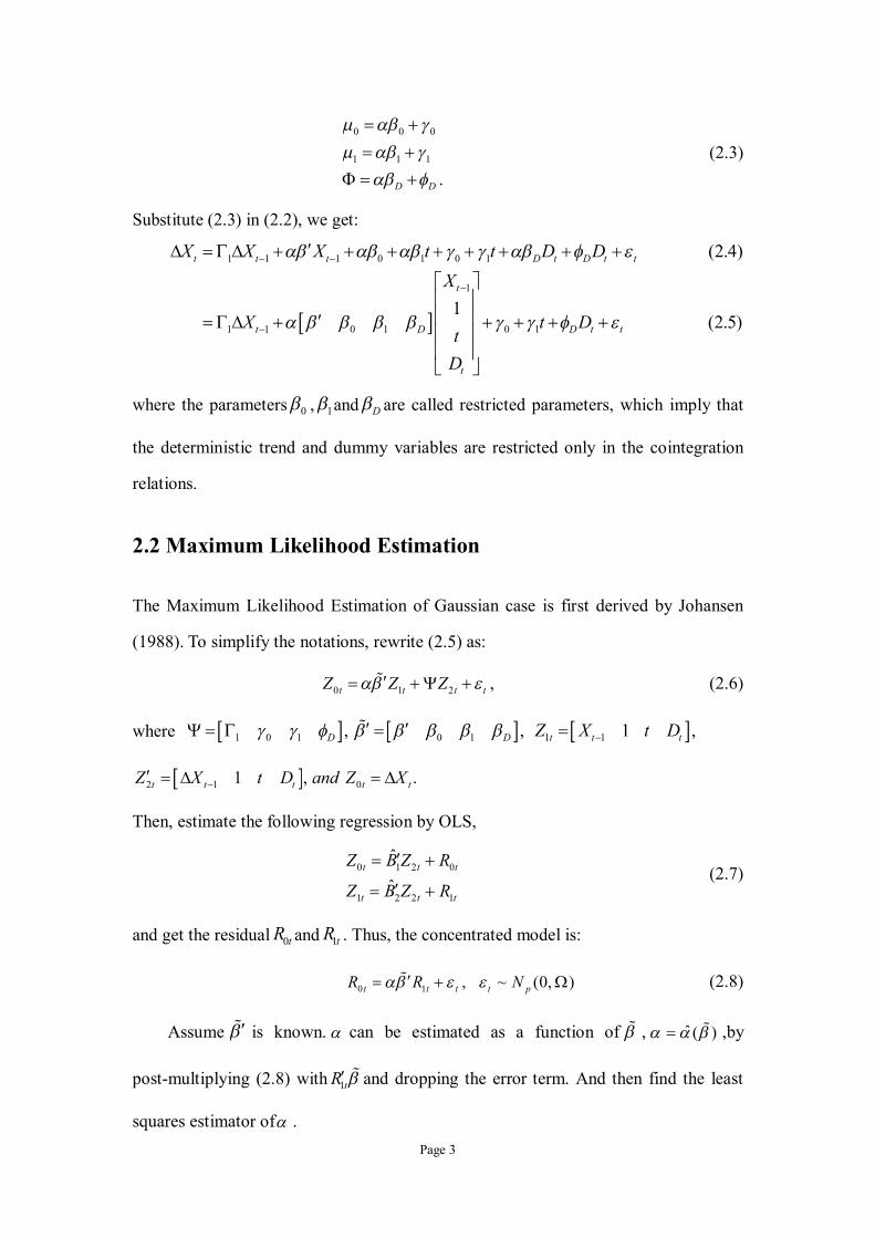
Substitute (2.3) in (2.2), we get:

1 1 1 0 1 0 1

1

1 1 0 1 0 1

(2.4)

1(2.5)

t t t D t D t t

t

t D D t t

t

X X X t t D DX

X t Dt

D

where the parameters 0 , 1 and D are called restricted parameters, which imply that

the deterministic trend and dummy variables are restricted only in the cointegration

relations.

2.2 Maximum Likelihood Estimation

The Maximum Likelihood Estimation of Gaussian case is first derived by Johansen

(1988). To simplify the notations, rewrite (2.5) as:

0 1 2 ,t t t tZ Z Z (2.6)

where 1 0 1 0 1 1 1, , 1 ,D D t t tZ X t D

2 1 01 , .t t t t tZ X t D and Z X

Then, estimate the following regression by OLS,

0 1 2 0

1 2 2 1

ˆ

ˆt t t

t t t

Z B Z R

Z B Z R

(2.7)

and get the residual 0tR and 1tR . Thus, the concentrated model is:

0 1 , ~ (0, )t t t t pR R N (2.8)

Assume is known. can be estimated as a function of , ˆ ( ) ,by

post-multiplying (2.8) with 1tR and dropping the error term. And then find the least

squares estimator of .

Page 4

0 1 1 1t t t tR R R R (2.9)

101 11 ij it jtt

S S where S T R R (2.10)

101 11ˆ ( ) ( )S S (2.11)

The error covariance matrix ̂ as a function of fixed and is shown in (2.12),

100 01 10 11 00 01 11 10

ˆ ( ) .S S S S S S S S (2.12)

Under the multivariate normality assumption, maximizing the likelihood function of

(2.8) is equivalent to minimizing the determinant of ̂ : 1

11 10 00 0100

11

( )ˆ .S S S S

SS

(2.13)

Then (2.13) can be minimized by solving the eigenvalue problem as follows,

111 10 00 01 0.S S S S (2.14)

The minimum of ̂ is:

00min1

ˆ (1 ) .p

ii

S

(2.15)

Finally, the maximum likelihood estimation of i is obtained by normalizing the

corresponding eigenvector of i .The magnitude of is a measure of the “stationary”

of the corresponding 1tX , the larger the i is, the “more” stationary the relation is.

When 0i , the corresponding linear combination 1i tX is non-stationary.

2.3 Trace Test

To determine the number of non-zero eigenvalue, namely the cointegration rank, trace

test is introduced by Johansen (1991). The null hypothesis of trace test is:

H0: Rank≤r, namely, there exist r cointegration relation at most.

The trace test uses the idea of likelihood ratio test. The test statistic p r is:

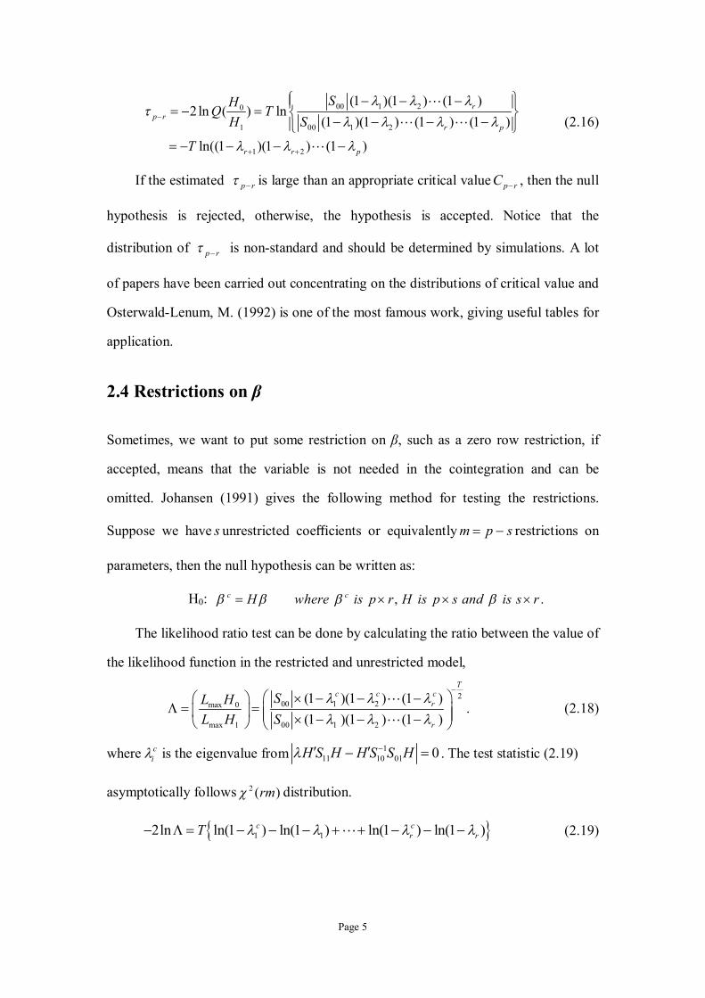
Page 5

00 1 20

1 00 1 2

1 2

(1 )(1 ) (1 )2 ln ( ) ln

(1 )(1 ) (1 ) (1 )

ln((1 )(1 ) (1 )

rp r

r p

r r p

SHQ TH S

T

(2.16)

If the estimated p r is large than an appropriate critical value p rC , then the null

hypothesis is rejected, otherwise, the hypothesis is accepted. Notice that the

distribution of p r is non-standard and should be determined by simulations. A lot

of papers have been carried out concentrating on the distributions of critical value and

Osterwald-Lenum, M. (1992) is one of the most famous work, giving useful tables for

application.

2.4 Restrictions on β

Sometimes, we want to put some restriction on β, such as a zero row restriction, if

accepted, means that the variable is not needed in the cointegration and can be

omitted. Johansen (1991) gives the following method for testing the restrictions.

Suppose we have s unrestricted coefficients or equivalently m p s restrictions on

parameters, then the null hypothesis can be written as:

H0: , .c cH where is p r H is p s and is s r

The likelihood ratio test can be done by calculating the ratio between the value of

the likelihood function in the restricted and unrestricted model,

200 1 2max 0

max 1 00 1 2

(1 )(1 ) (1 ).

(1 )(1 ) (1 )

Tc c c

r

r

SL HL H S

(2.18)

where ci is the eigenvalue from 1

11 10 01 0H S H H S S H . The test statistic (2.19)

asymptotically follows 2 ( )rm distribution.

1 12ln ln(1 ) ln(1 ) ln(1 ) ln(1 )c cr rT (2.19)

Page 6

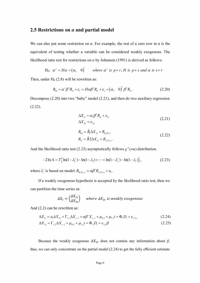
2.5 Restrictions on α and partial model

We can also put some restriction on α. For example, the test of a zero row in α is the

equivalent of testing whether a variable can be considered weakly exogenous. The

likelihood ratio test for restrictions on α by Johansen (1991) is derived as follows:

H0: 1 0 ,c cH where is p r H is p s and is s r

Then, under H0 (2.8) will be rewritten as:

0 1 1 1 10 .ct t t t t tR R H R R (2.20)

Decompose (2.20) into two “baby” model (2.21), and then do two auxiliary regression

(2.22).

1 1 1 1

2 2

t t t

t t

X RX

(2.21)

0 1 2 0,

1 2 1,

ˆ

ˆ 2 .t t H t

t t H t

R B X R

R B X R

(2.22)

And the likelihood ratio test (2.23) asymptotically follows 2 ( )rm distribution.

1 12ln ln(1 ) ln(1 ) ln(1 ) ln(1 ) ,c cr rT (2.23)

where ci is based on model: 0, 1,H t H t tR R u .

If a weakly exogenous hypothesis is accepted by the likelihood ratio test, then we

can partition the time series as:

훥푋 = 훥푋훥푋                         푤ℎ푒푟푒      훥푋     푖푠    푤푒푎푘푙푦    푒푥표푔푒푛표푢푠

And (2.2) can be rewritten as:

1 1 2 1.1 1 1 0.1 1.1 1 1.2,

2 1.2 1 0.2 1.2 2 2,

(2.24)(2.25)

t t t t t t

t t t t

X a X X X t DX X t D

Because the weakly exogenous 훥푋 does not contain any information about β,

thus, we can only concentrate on the partial model (2.24) to get the fully efficient estimate

Page 7

4.5

6.5

8.5

10.5

12.5

14.5 Original Data

-0.4-0.3-0.2-0.1

00.10.20.30.40.5

1830 1861 1889 1920 1950 1981

Differenced Data

of β. Juselius (2006) shows that a partial system has more stable parameters than the full

system because the noise of weakly exogenous variables a not included.

3. Data

The original data is the Swedish national accounts data collected by Department

of Economic History, Stockholm University. This thesis mainly uses five series: Final

Consumption, Investment, Export, Import and Gross Domestic Product, range from

1830 to 2000. All the series are Nominal values measured in purchasers’ prices,

million SEK. Import and export are recorded on the c.i.f./f.o.b.-basis[1] and GDP are

calculated by expenditure. Logarithm is applied to all variables.

3.1 Final Consumption

The Final Consumption measures the value of goods and services consumed by both

private and government. The original data in Figure 3.1 left shows a time trend of

increasing while the differenced data in Figure 3.1 right move in a tight range around

a constant. Then it can be suggested that the Final Consumption may be a random

walk with drift. It`s noticeable that a sharp wave appears in 1914- 1920, due to the

outbreak of World War I. The war pushes up the consumption and then gives a

Figure 3.1 Logarithm Final Consumption

[1] c.i.f./f.o.b: Cost Insurance and Freight / Free On Board

Page 8

1.5

3.5

5.5

7.5

9.5

11.5

13.5

1830 1861 1889 1920 1950 1981

Original Data

-0.5

-0.3

-0.1

0.1

0.3

0.5

0.7

1830 1861 1889 1920 1950 1981

Differenced Data

strongly negative impact during the post-war time. The same shape of wave around

1944 can be explained by the World War II in similar way.

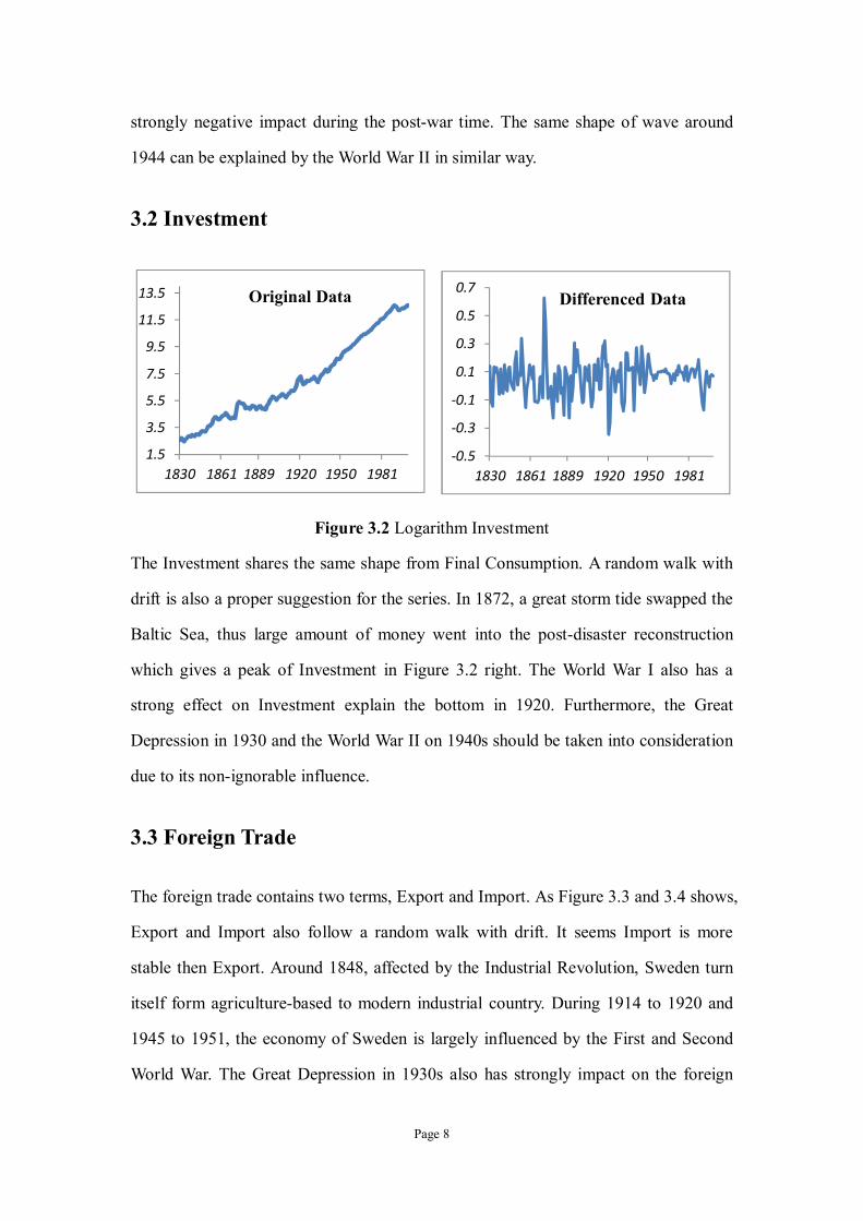
3.2 Investment

Figure 3.2 Logarithm Investment

The Investment shares the same shape from Final Consumption. A random walk with

drift is also a proper suggestion for the series. In 1872, a great storm tide swapped the

Baltic Sea, thus large amount of money went into the post-disaster reconstruction

which gives a peak of Investment in Figure 3.2 right. The World War I also has a

strong effect on Investment explain the bottom in 1920. Furthermore, the Great

Depression in 1930 and the World War II on 1940s should be taken into consideration

due to its non-ignorable influence.

3.3 Foreign Trade

The foreign trade contains two terms, Export and Import. As Figure 3.3 and 3.4 shows,

Export and Import also follow a random walk with drift. It seems Import is more

stable then Export. Around 1848, affected by the Industrial Revolution, Sweden turn

itself form agriculture-based to modern industrial country. During 1914 to 1920 and

1945 to 1951, the economy of Sweden is largely influenced by the First and Second

World War. The Great Depression in 1930s also has strongly impact on the foreign

Page 9

-1.2

-0.7

-0.2

0.3

0.8

1.3

1830 1861 1889 1920 1950 1981

Differenced Data

trade.

Figure 3.3 Logarithm Export

Figure 3.4 Logarithm Import

3.4 Gross Domestic Product

Gross Domestic Product measures the market value of all final goods and services,

and is calculated by expenditure approach. It`s the most important indicator of a

country's standard of living and represent the overall power of economy.

Figure 3.5 shows that the GDP of Sweden has firm growth during the past 170

years. The historical events also have great impact so that the data is very unstable if

events occurred. During the war time, a shape ware is recorded because of the military

needs and the change of outside environment. Around 1930s, the Great Depression

also strongly influent the economy of Sweden, cause a low bottom in the differenced

data.

-0.9-0.7-0.5-0.3-0.10.10.30.50.7 Differenced Data

2468

10121416

1830 1861 1889 1920 1950 1981

Original Data

1.5

3.5

5.5

7.5

9.5

11.5

13.5

15.5

1830 1861 1889 1920 1950 1981

Original Data

Page 10

4

6

8

10

12

14

16

1830 1861 1889 1920 1950 1981

Original Data

Figure 3.5 Gross Domestic Product

4. Results

4.1 Unit Root Test

The notation of variables is given in Appendx I. Although the shape of lines of each

variabe suggest I(1) process is reasonable, it`s still necessary to test unit-root with

Augmented Dickey–Fuller F test. The result in Table 4.1 strongly indicates that all the

series are I(1) process.

Table 4.1 Augmented Dickey–Fuller test

Data Series Type of test ADF P-Value

Before Difference

FC With Constant, Without trend 0.99

INV With Constant, Without trend 0.99

EX With Constant, Without trend 0.99

IM With Constant, Without trend 0.99

GDP With Constant, Without trend 0.99

After Difference

FC Without Constant and Trend 0.01

INV Without Constant and Trend 0.01

EX Without Constant and Trend 0.01

IM Without Constant and Trend 0.01

GDP Without Constant and Trend 0.01

-0.35

-0.25

-0.15

-0.05

0.05

0.15

0.25

0.35

1830 1861 1889 1920 1950 1981

Differenced Data

Page 11

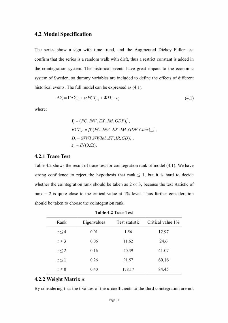
4.2 Model Specification

The series show a sign with time trend, and the Augmented Dickey–Fuller test

confirm that the series is a random walk with dirft, thus a restrict constant is added in

the cointegration system. The historical events have great impact to the economic

system of Sweden, so dummy variables are included to define the effects of different

historical events. The full model can be expressed as (4.1).

1 1t t t t tY Y ECT D (4.1)

where:

1 1

( , , , , ) ,

( , , , , , ) ,

( , , , , ) ,~ (0, ).

t t

t t

t t

t

Y FC INV EX IM GDP

ECT FC INV EX IM GDP Cons

D WWI WWIob ST IR GDIN

4.2.1 Trace Test

Table 4.2 shows the result of trace test for cointegration rank of model (4.1). We have

strong confidence to reject the hypothesis that rank ≤ 1, but it is hard to decide

whether the cointegration rank should be taken as 2 or 3, because the test statistic of

rank = 2 is quite close to the critical value at 1% level. Thus further consideration

should be taken to choose the cointegration rank.

Table 4.2 Trace Test

Rank Eigenvalues Test statistic Critical value 1%

r ≤ 4 0.01 1.56 12.97

r ≤ 3 0.06 11.62 24.6

r ≤ 2 0.16 40.39 41.07

r ≤ 1 0.26 91.57 60.16

r ≤ 0 0.40 178.17 84.45

4.2.2 Weight Matrix α

By considering that the t-values of the α-coefficients to the third cointegration are not

Page 12

very significant in Table 4.3, so rank = 2 is a preferable choice for the Swedish data.

Also, the t-values of INV is not significant in the first two columns, which suggests

that INV might be weakly exogenous such that we can replace the full model with a

partial model.

Table 4.3 Weight Matrix α

α1 α2 α3 α4 α5

FC 0.51[6.36] -0.10[-2.42] -0.45[-3.94] 0.01[0.25] 0.00[0.01]

INV 0.35[1.78] -0.08[-0.73] -0.21[-0.59] -0.2[-2.10] 0.08[0.87]

EX 0.93[4.40] -0.58[-5.12] 0.51[1.69] -0.14[-1.40] -0.03[-0.34]

IM 2.44[9.30] 0.06[0.40] -0.05[-0.14] -0.16[-0.22] -0.03[0.00]

GDP 0.39[5.37] -0.20[-5.05] -0.19[-1.84] 0.00[0.13] 0.02[0.00]

Note: T-values are given in the bracket, bolded if |t-value| > 2

4.2.3 Cointegrating Vectors β

According to the economic theory, Final Consumption is the main force of promoting

the growth of Gross Domestic Product, so it`s reasonable to assume that they are

homogeneous. The estimated cointegrating vectors β is given in Table 4.4 and it is

easy to get that FC and GDP has a firm relation in the first two cointegration relations:

FC = -0.9×GDP.

Table 4.4 Cointegrating Vectors β

β1 β2 β3 β4 β5 β6

FC 1.00 1.00 1.00 1.00 1.00 1.00

INV 0.19 0.14 0.10 0.30 -0.01 -1.31

EX 0.43 0.40 -0.01 0.24 0.42 0.35

IM -0.51 -0.43 -0.04 -0.12 -0.20 0.13

GDP -1.11 -1.12 -1.03 -1.45 -1.21 0.26

Cons 0.42 0.40 0.16 1.18 0.56 -5.84

Note: Normalized with respect to the first row. Cons represent the constant in cointegration.

Page 13

4.2.4 Test for Restrictions on β and α

Testing the hypothesis raised in the previous section can be done by put

corresponding restrictions on the parameters. Matrix HB and HA will be used to

restrict β and α when testing the weakly exogenous and homogeneous hypothesis.

H1: FC = -0.9×GDP

H2: INV is weakly exogenous.

0 0 0 0.9 01 0 0 0 00 1 0 0 00 0 1 0 00 0 0 1 00 0 0 0 1

HB

1 0 0 00 0 0 00 1 0 00 0 1 00 0 0 1

HA

The results of likelihood ratio test for restrictions are given in Table 4.5. The

p-values of tests suggest that both H1 and H2 are accepted. Instead of the full model

(4.1), a partial model (4.2) is estimated due to the weakly exogenous of INV.

Table 4.5 Restriction Test

Hypothesis LR statistic P-value Chi square df

H1 0.04 0.98 2

H2

H1 and H2

3.42

3.42

0.18

0.18

2

2

4.3 Estimation

The estimated partial model is given in (4.2) under the homogeneous and weakly

exogenous conditions.

4.4 Fitted Values and Residuals Diagnostics

Fitted values and residuals plots are given in Figure 4.1. We can see that the fitted

values in dotted line are almost coincided with the original data. And the R-square of

the VECM are all larger than 0.6 also indicating that the model fitted well. The results

of ARCH test for heteroscedasticity, Portmanteau test for serially correlated errors

Page 14

[0.394] [ 0.143] [0.306] [0.455] [1.876]

[0.825] [ 1.203] [0.881] [0.721] [ 1.409]

[0.999] [ 0.359] [0.730] [

0.075 0.006 0.016 0.019 0.440

0.406 0.125 0.118 0.077 0.855

0.584 0.044 0.117 0.218

t

t

t

t

FCEXIMGDP

1

1

1

1.721] [ 1.392]1

1[0.942] [ 0.591] [1.238] [0.281] [1.027]

[5.429] [ 2.277]

1.004

0.143 0.019 0.051 0.009 0.192

0.486 0.088

0.8

t

t

t

t

t

FCINVEXIMGDP

1

[3.733] [ 4.954]

[8.684] [0.345]

[4.655] [ 5.273]

64 0.495 1 0.189 0.418 0.493 1.111 0.4282.390 0.041 1 0.129 0.419 0.448 1.111 0.386

0.332 0.163

tFCINV

1

1

1

1

[3.115] [8.454] [2.214]

[2.437] [5.597] [4.864]

[4.274] [5.254]

[6.592] [8.268]

(4.2)

0.102 0.341 0.088

0.207 0.584 0.502

0.432 0.652 0.

0.173 0.266

t

t

t

t

t

EXIMGDPCons

INV

[ 0.256] [ 1.440] [ 0.105] [ 0.186]

[0.166] [5.473] [ 3.421]

[3.248] [ 0.644] [ 1.373] [ 0.801]

[3.896] [ 0.376] [2.016] [ 0.996]

0.011 0.041 0.004 0.008

0.019 0.404 0.356 0.

398 0.089 0.121 0.099

0.124 0.013 0.046 0.032

,

[ 3.036] ,

,[ 1.183]

,[ 1.770]

ˆ320 ˆ

ˆ0.148ˆ0.057

FC t

EX t

IM t

GDP t

WWIWWIob

STWWII

IRGD

and Jarque-Bera tests for normality are given in Table 4.6. All the tests are accepted at

1% level, thus the model is well specified.

Table 4.6 Residual test

ARCH Normality R-square Portmanteau Test

FC 0.023 0.314 0.814

0.1035 EX 0.027 0.295 0.602

IM 0.431 0.625 0.669

GDP 0.808 0.335 0.862

4.5 Interpretation

The estimated model (4.2) gives the coefficients with t-values in the bracket under

the homogeneous and weakly exogenous conditions in section 4.2.

Matrix Г shows the short-run dynamic relation of each variables. The most

Page 15

(a) (b

) (d

)

(c)

Figu

re 4

.1 F

itted

val

ue in

upp

er g

raph

and

resi

dual

in lo

wer

gra

ph. (

a) fo

r FC

, (b)

for E

X, (

c) fo

r IM

and

(d) f

or G

DP.

Page 16

significant relations are that change of FC positively depends on the change in GDP

of last year, and change of IM will follows the same trend of last term.

The trace test suggests cointegration rank is 2, and the corresponding error

correction terms are:

1 1 1 1 1 1

2 1 1 1 1 1

0.189 0.418 0.493 1.111 0.4280.129 0.419 0.448 1.111 0.386

t t t t t

t t t t t

ECT FC INV EX IM GDPECT FC INV EX IM GDP

(4.1)

Since the error correction terms is stationary time series, so the existence of

cointegration relation offer support to the Swedish economic long-run stability. The

highly significant loading matrix α indicates that the error correction terms play a vital

role in the VECM model.

The coefficients in ρ describe the relations of the weakly exogenous INV and the

rest series. The t-value of ρ are larger than 2.4 suggests INV has great influence on the

economic system.

The Ф matrix shows the impact of different historical event on the series. The

most influential event is the World War I, which affects all the series significantly, and

the EX is the most sensitive indicator which is under the influence of all but ST.

5. Conclusions

This paper aims to find the cointegration relationship lying in the Swedish economy

and interpret the economic meaning. First, we present that the series follow a random

walk process with Augmented Dickey–Fuller test. And then, specify the full model

with restricted constant to represent the deterministic time trend and a number of

dummy variables to eliminate the unreasonable changes in time series caused by

major historical events. After that, the hypothesis of weakly exogenous for INV and

homogeneous for FC and GDP are accepted by doing likelihood ratio test for

restrictions on parameters. In the end, we achieve the most important result: the

Swedish national account has cointegration relations and the cointegration system

have considerable effect on the economy. This result gives support to the long-run

Page 17

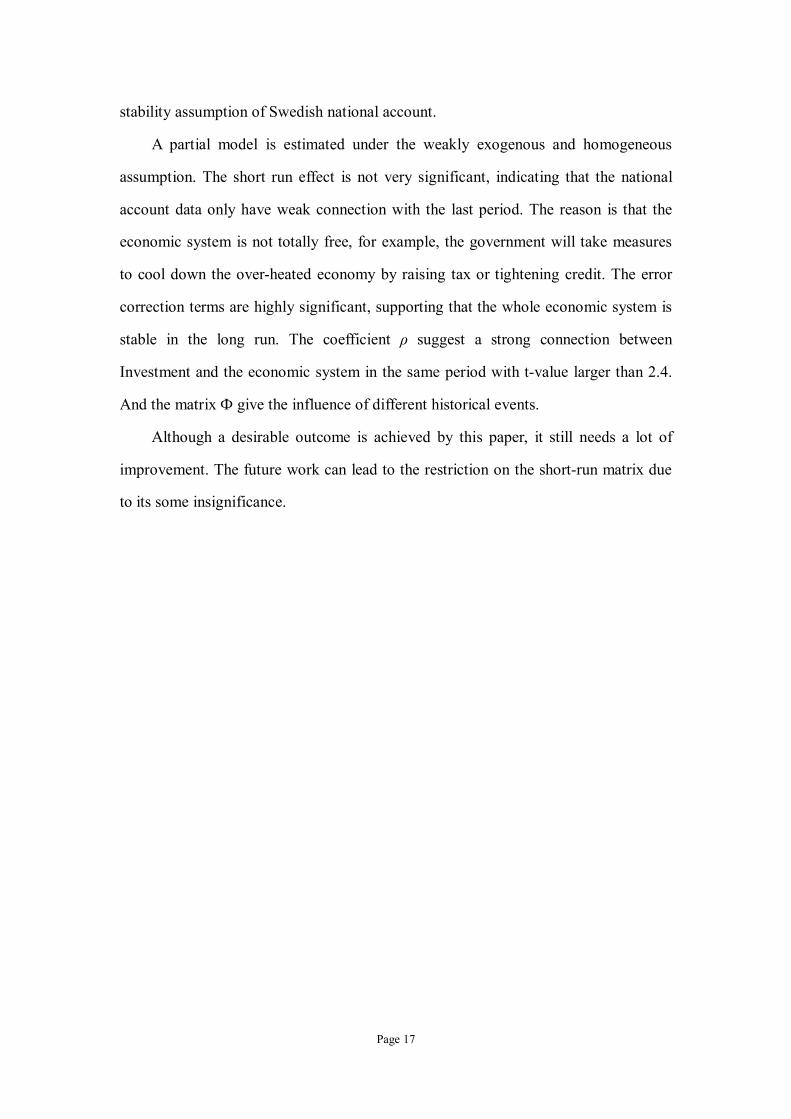
stability assumption of Swedish national account.

A partial model is estimated under the weakly exogenous and homogeneous

assumption. The short run effect is not very significant, indicating that the national

account data only have weak connection with the last period. The reason is that the

economic system is not totally free, for example, the government will take measures

to cool down the over-heated economy by raising tax or tightening credit. The error

correction terms are highly significant, supporting that the whole economic system is

stable in the long run. The coefficient ρ suggest a strong connection between

Investment and the economic system in the same period with t-value larger than 2.4.

And the matrix Ф give the influence of different historical events.

Although a desirable outcome is achieved by this paper, it still needs a lot of

improvement. The future work can lead to the restriction on the short-run matrix due

to its some insignificance.

Page 18

Reference

[1] Engle R.F. & Granger C.W.J., 1987. Cointegration and Error Correction:

Representation, Estimation, and Testing. Econometrica, 55(2), pp. 251-276.

[2] Granger, C.W. J. 1981. Some properties of time series data and their use in

econometric model specification. Journal of Econometrics, 16, 121–130.

[3] Granger, C.W. J. 1983. Cointegrated Variables and Error Correction Models.

Discussion Paper, 83-13a, University of California, San Diego.

[4] Granger, C.W. J. and Weiss, A. A. 1983. Time Series Analysis of Error-Correction

Models. Studies in Econometrics, Time Series and Multivariate Statistics, ed. by S.

Karlin, T. Amemiya and L. A. Goodman. New York: Academic Press, pp. 255—278.

[5] Hamilton, J.D., 1994. Time Series Analysis. Princeton, NJ: Princeton University

Press.

[6] Katarina Juselius, 2006. The Cointegrated VAR Model: Methodology and

Applications. Oxford University Press.

[7] Osterwald-Lenum, M. 1992. A Note with Quantiles of the Asymptotic Distribution

of the Maximum Likelihood Cointegration Rank Test Statistics. Oxford Bulletin of

Economics and Statistics, 55, 3, 461–472.

[8] Soren Johansen, 1988. Statistical Analysis of cointegration Vectors. Journal of

Economic Dynamics and Control, pp.234-254

[9] Soren Johansen, 1991. Estimation and Hypothesis Testing of Cointegration

Vectors in Gaussian Vector Autoregressive Models. Econometrica, Vol.59, No.6, pp.

1551-1580.

Page 19

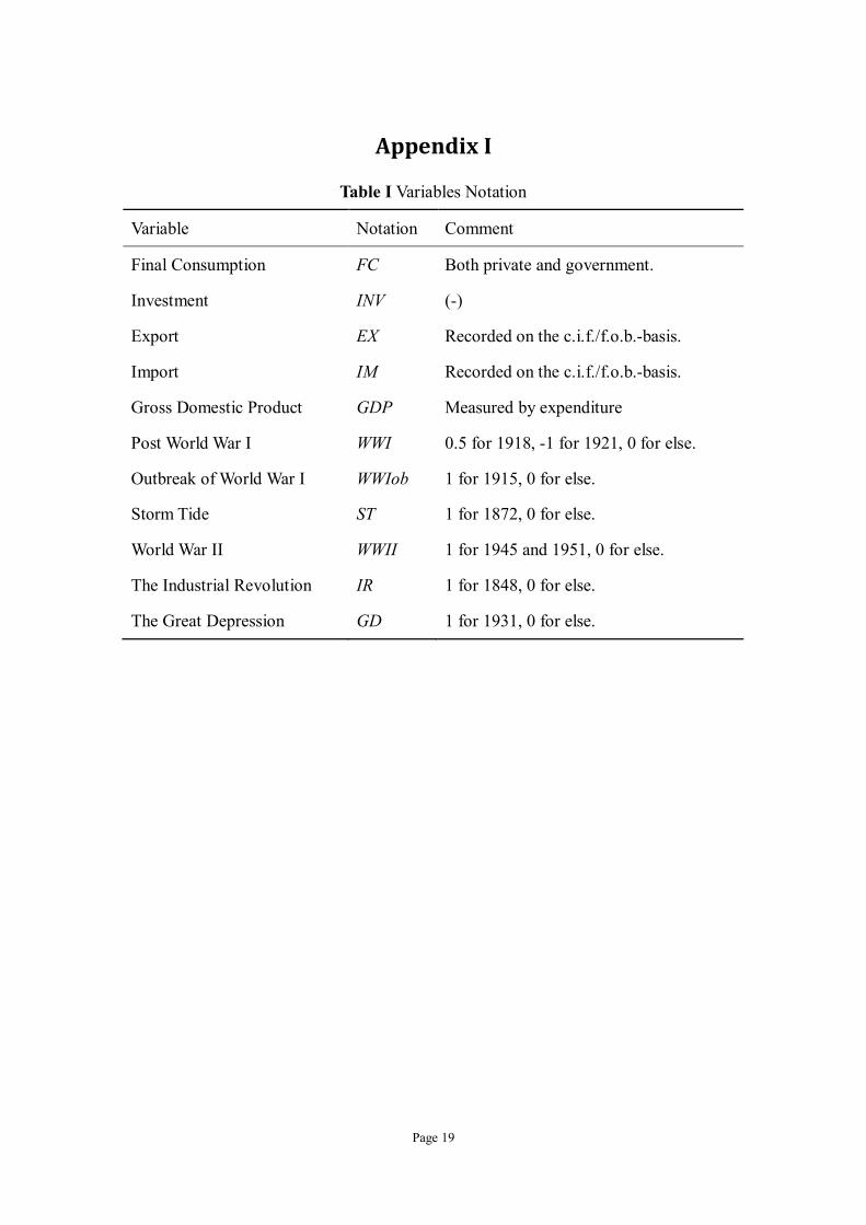
Appendix I

Table I Variables Notation

Variable Notation Comment

Final Consumption FC Both private and government.

Investment INV (-)

Export EX Recorded on the c.i.f./f.o.b.-basis.

Import IM Recorded on the c.i.f./f.o.b.-basis.

Gross Domestic Product GDP Measured by expenditure

Post World War I WWI 0.5 for 1918, -1 for 1921, 0 for else.

Outbreak of World War I WWIob 1 for 1915, 0 for else.

Storm Tide ST 1 for 1872, 0 for else.

World War II WWII 1 for 1945 and 1951, 0 for else.

The Industrial Revolution IR 1 for 1848, 0 for else.

The Great Depression GD 1 for 1931, 0 for else.