Research Division Federal Reserve Bank of St. Louis Working Paper Series

Explaining China’s Trade Imbalance Puzzle

Yi Wen

Working Paper 2011-018A http://research.stlouisfed.org/wp/2011/2011-018.pdf

August 2011

FEDERAL RESERVE BANK OF ST. LOUIS Research Division

P.O. Box 442 St. Louis, MO 63166

______________________________________________________________________________________

The views expressed are those of the individual authors and do not necessarily reflect official positions of the Federal Reserve Bank of St. Louis, the Federal Reserve System, or the Board of Governors.

Federal Reserve Bank of St. Louis Working Papers are preliminary materials circulated to stimulate discussion and critical comment. References in publications to Federal Reserve Bank of St. Louis Working Papers (other than an acknowledgment that the writer has had access to unpublished material) should be cleared with the author or authors.

Explaining China�s Trade Imbalance Puzzle�

Yi WenFederal Reserve Bank of St. Louis

&Tsinghua University

This Version: October 12, 2011

Abstract

The current global-imbalance literature (which explains why capital �ows from poor to rich

countries) is unable to explain China�s foreign asset positions because capital cannot �ow out

of China under capital controls. Hence, this literature has not succeeded in explaining China�s

large and persistent trade imbalances with the United States. A closely related but deeper

puzzle that this literature fails to address is China�s high household saving rate despite an

astonishingly rapid income growth rate. This paper shows that a modi�ed (and calibrated)

Melitz (2003) model can qualitatively and quantitatively explain China�s trade surplus and its

massive accumulation of low-yield foreign reserves. The simple in�nite-horizon model is also

consistent with the stylized fact that high saving is the consequence of high growth (Modigliani

and Cao, 2004), which the permanent income theory and global-imbalance literature fail to

predict.

Keywords: Chinese Economy, Foreign Reserve, High Saving Rate Puzzle, Global Imbalance,

US Trade De�cit.

JEL Codes: E21, F11, F30, F41, F43, O16.

�This is a substantially revised version of my earlier working papers (Wen, 2009a, 2011). I am grateful to B.Ravikumar for his detailed comments and suggestions. I also thank Franklin Allen, David Andolfatto, Kaiji Chen,Nicolas Coeurdacier, Silvio Contessi, Yannick Kalantzis, Nobu Kiyotaki, Narayana Kocherlakota, Patrick Pintus,Zheng Song, Mark Spiegel, Shang-Jin Wei, Xiaodong Zhu, and seminar participants at the Federal Reserve Bankof St. Louis, the 2010 Conference on Chinese Economy (Shanghai), the Marseille Conference on "Asset Prices,Credit and Macroeconomic Policies", the 2011 System Committee on International Economic Analysis at the AtlantaFed, and the Columbia-Tsinghua Workshop in International Economics 2011 for comments. I also thank MingyuChen and Xin Wang for research assistance and Judy Ahlers for editorial assistance. The usual disclaimer applies.Correspondence: Yi Wen, Research Department, Federal Reserve Bank of St. Louis, St. Louis, MO, 63104. Phone:314-444-8559. Fax: 314-444-8731. Email: yi.wen@stls.frb.org.

1

1 Introduction

Recent advances in international trade theory attempt to explain the patterns of trade at the

country, industry, and �rm levels.1 However, it has little to o¤er on the question of why trade

may be imbalanced between countries over a prolonged period. According to Deardor¤ (2010),

standard trade theories cannot explain why developing countries (such as China) with comparative

advantages in producing future goods have been running trade surpluses while industrial nations

(such as the United States) with comparative advantages in producing present goods are running

trade de�cits. That is, from the viewpoint of the current trade theories, the steady increase in

China�s trade balance from a small de�cit (-$1.1 billion) in 1978 (the beginning year of economic

reform) to a gigantic surplus ($400 billion) in the �rst half of 2009 is a puzzle.2

The international �nance approach to the trade imbalance puzzle is to model conditions under

which China�s domestic savings exceed domestic investment so that China should experience capital

out�ows. Between 1978 and 2009, China�s foreign exchange reserves (mostly U.S. dollars) increased

dramatically, from $2 billion to $2.4 trillion� a more than 1,000-fold expansion� making China the

world�s largest holder of foreign exchange reserves. Consequently, the accounting identity between

the current account and the capital account implies that China automatically runs a trade surplus.3

Such an approach faces two fundamental challenges. First, why is China�s astonishing 45%

investment-to-GDP ratio not able to fully absorb its domestic savings? How can the notoriously

high household saving rate in China be explained when household income has been growing at 10%

per year and the real return to household saving is negative? Second, even if a su¢ ciently high

saving rate in excess of the investment rate can be generated by a model, such a saving-investment

imbalance may still run counter to China�s reality: (i) If domestic savings generated from the model

are in the form of �xed capital, then the model would predict out�ows from China to developed

countries in the form of foreign direct investment (FDI). However, the reality indicates the opposite:

it is the industrial economies that have been sending FDI to China over the past few decades. (ii)

If the excess domestic savings are in the form of local currency or demand deposits, such �nancial

capital cannot leave China because China has capital controls and the renminbi (RMB) is not

internationally convertible. To purchase U.S. government bonds, for example, Chinese savers must

�rst have dollars in hand. Therefore, to explain China�s trade surplus through an international-

1See, e.g., the seminal works of Bernard, Eaton, Jensen, and Kortum (BEJK, 2004), Chaney (2008), Melitz (2003),and the rapidly growing literature following these papers.

2The bulk of the surplus results from trade with the U.S. and takes the form of �nal consumption goods.3See, Caballero, Farhi, and Gourinchas (2008); Mendoza, Quadrini, and Rios-Rull (2009); and Song, Storesletten,

and Zilibotti (2011), among others.

2

�nance approach, the "excess savings" must be in the form of consumption goods instead of assets.

But this conclusion revisits the trade imbalance puzzle: Why is China exporting more goods than

it is importing?

Resolving the trade imbalance puzzle thus requires not only starting with a basic trade frame-

work with exporters as the main actors, but also �nd new ways to model the micro-incentives for the

demand of low-yield liquid assets (such as dollars and U.S. government bonds). Conventional ap-

proaches to model the demand for low-yield assets, such as those with cash-in-advance constraints or

money-in-the-utility assumptions, are inadequate since the optimal asset demand in such models is

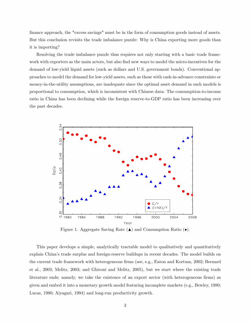
proportional to consumption, which is inconsistent with Chinese data: The consumption-to-income

ratio in China has been declining while the foreign reserve-to-GDP ratio has been increasing over

the past decades.

Figure 1. Aggregate Saving Rate (N) and Consumption Ratio (�).

This paper develops a simple, analytically tractable model to qualitatively and quantitatively

explain China�s trade surplus and foreign-reserve buildups in recent decades. The model builds on

the current trade framework with heterogeneous �rms (see, e.g., Eaton and Kortum, 2002; Bernard

et al., 2003; Melitz, 2003; and Ghironi and Melitz, 2005), but we start where the existing trade

literature ends; namely, we take the existence of an export sector (with heterogeneous �rms) as

given and embed it into a monetary growth model featuring incomplete markets (e.g., Bewley, 1980;

Lucas, 1980; Aiyagari, 1994) and long-run productivity growth.

3

Our theory predicts that when exporters (i) face uninsured risks that remain constant over

time as income grows and (ii) are subject to borrowing constraints, their marginal propensity to

save increases with income growth. That is, the more income they earn, the larger portion of the

income will they save, in sharp contrast to the conventional wisdom based on Friedman�s (1957)

permanent income hypothesis (PIH). Indeed, during the 30 years of China�s rapid economic growth,

its private consumption-to-GDP ratio has fallen from roughly 50% in 1980 to 35% in 2008 (see the

C/Y ratio in Figure 1), while government spending as a fraction of total national income has

remained roughly constant at about 14%. Thus, Chinese consumers have reduced their propensity

to consume signi�cantly despite the rapidly rising per capita income. China�s national saving rate

(private investment plus net exports over GDP) has also increased steadily over the past 30 years,

from 34% to 51% (see the (I+NX)/Y ratio in Figure 1).

Figure 2. Household Saving Ratio (left scale) and Income Growth (right scale)

Our model is also consistent with a well-known stylized fact that is not well explained by the

existing literature: Lagged income growth is a strong predictor of future saving rates� or high

saving is the consequence of high growth (e.g., Modigliani and Cao, 2004). Figure 2 depicts the

household saving ratio (blue diamonds, left axis) and the long-term growth rate of household income

(red squares, right axis) for the 1953-2006 period. The household saving rate is de�ned as the ratio

between net wealth changes and disposable income, and the long-term income-growth rate is de�ned

as the average growth rate of household income of the past 14 years, following Modigliani and Cao

4

(2004). The �gure shows that the household saving rate tracks the past average income growth rate

very closely and has increased steadily since 1978. The average saving rate was about 5% before

1978 when the average income growth rate was about 2% per year. After the economic reform, the

saving rate increased to over 35% after 1994 when the average rate of household income growth

reached near 10% per year. The extraordinary Chinese saving rate and its positive association with

income growth are not unique. Similar high saving rates have also been observed in other emerging

economies during their rapid-growth periods, such as Japan in the 1960-70s, Hong Kong in the

1980s, and Taiwan and South Korea in the 1990s (see, e.g., Wang and Wen, 2011).

Our analysis suggests that given the elastic labor supply from China�s rural areas and the rapid

growth in export income (e.g., due to a comparative advantage in labor costs and an expanding

world market for Chinese goods), �nancial frictions in China will naturally lead to massive trade

surplus and foreign-reserve buildups. The faster the export income grows, the larger is the foreign

reserve-to-GDP ratio. In fact, China�s total imports-to-exports ratio has fallen during the fast-

growth period, from 1.6 in 1985 to around 0.8 in 2008. That is, while exports have grown at

a double-digit annual rate, total imports have failed to keep pace. As a result, China�s trade

surplus and foreign reserves have exploded. Therefore, the data suggest that Chinese households

might have been saving an increasingly larger portion of their income (including dollars earned from

international trade) to provide the safety net and self-insurance unavailable to them from markets.4

Such a precautionary saving motive is also supported by the fact that the bulk of the household

saving in China consists of bank deposits despite low interest rates.5 The average real interest rate

in China remained essentially at zero or negative values in the post-reform period. For example,

the average nominal 3-month deposit rate was 3.3%, the average 1-year rate was 5.6% (see the line

with green triangles in Figure 2, left axis), while the average in�ation rate was about 6% in the

1991-2007 period.6

Many analysts believe that the steady increase in America�s trade de�cit with China is the

consequence of a signi�cantly undervalued Chinese currency. In other words, Chinese goods are

too cheap relative to American goods. Hence, Americans can buy many Chinese goods while the

Chinese can barely a¤ord American goods. Indeed, some economists and politicians in the U.S. have

alleged that the Chinese government has been manipulating its currency to deliberately achieve a

large trade surplus and an excessive amount of foreign reserves. This paper argues that the trade

4Even though China has experienced impressive economic growth over the past 30 years since its economic reformand entering the global marketplace, its �nancial reform has not kept pace with its economic growth. Because of thelack of social safety nets and severely underdeveloped insurance and �nancial markets, Chinese workers must saveexcessively (including dollars earned from international trade) to insure themselves against idiosyncratic uncertainty,such as bad income shocks, unemployment risk, accidents, and unexpected spending for housing, education, healthcare, and so on.

5Wen (2009b) shows that in China and India the share of cash and bank deposits accounts for more than 90% oftotal household �nancial wealth.

6Data for the interest rates before 1990 are not available.

5

imbalance puzzle has little to do with the real exchange rate.

The rest of the paper is organized as follows. Section 2 presents a benchmark model with

heterogeneous exporters (entrepreneurs) facing borrowing constraints and uninsured risks, charac-

terizes general equilibrium of the model, and derives decision rules for consumption, saving, and

production in closed form. Section 3 studies the relationship between the aggregate saving rate and

the income growth rate along a balanced growth path and a stochastic growth path, respectively.

Section 4 uses the model to predict China�s trade surplus and foreign-reserve buildups. Section

5 explores the implications of the model for other dimensions. Section 6 and Appendix B (not

for publication) discusses some robustness issues pertaining to the model structure and parameter

values. Section 7 reviews the related literature. Section 8 concludes the paper with remarks for

future research.

2 Benchmark Model

2.1 Caveats

Some important caveats are in order before we describe the model. A key assumption in this paper

is that idiosyncratic risk facing entrepreneurs remains constant over time despite long-run growth�

that is, the percentage changes in entrepreneur income (consumption) are stationary regardless of

the rate of income (consumption) growth. This assumption implies that idiosyncratic income shocks

have constant variances and are multiplicative to the income level but additive to the logarithm

of income. This assumption is consistent not only with the data but also with a large body of

the empirical and theoretical segments of the literature that measure and model idiosyncratic

uncertainty.7 In contrast, if idiosyncratic shocks are assumed to be additive to the income level

(instead of its logarithm), then idiosyncratic risk will diminish to zero on a balanced growth path,

rendering it irrelevant for the analysis.

Of course, a constant income risk implies that the variance of absolute income (i.e., the gap

between actual income level and its exponential growth trend) is increasing over time. However,

an increasing variance of the absolute income does not imply an increasing income risk because

the correct measure of risk is the percentage of �uctuations in income. A multiplicative shock to

the income trend simply means that the variance of logged income (i.e., the gap between logged

7A large body of the empirical literature �nds that the idiosyncratic component of logged household income(consumption) is stationary over time (see, e.g., DeBacker, Heim, Panousi, and Vidangos, 2010, Gottschalk andMo¢ tt, 1994, 2009; Mo¢ tt and Gottschalk, 1995, 2008; Haider, 2001, Heathcote, Perri, and Violante, 2010; Sabelhausand Song, 2009; Shin and Solon, 2008; among others). For example, using a large panel of tax returns from theInternal Revenue Service, DeBacker et al. (2010) �nd that the variance (volatility) of logged household income (aftercontrolling for time trend) has remained stationary over time in the United States for the period 1988-2006; namely,the standard deviation of percentage changes in income has not diminished but instead has remained constant forAmerican households.

6

income and its time trend) is constant over time.8 The question is this: Will rational entrepreneurs

(households) change their marginal propensity to save in a borrowing constrained economy when the

growth rate of their income changes but the income risk remains constant (that is, the �uctuations

in income remain constant relative to trend regardless of the growth rate)? It is precisely this

lack of such knowledge that has created the big puzzle regarding the high household saving rate in

China despite its well-known 10% per year income growth rate over the past few decades.9

Another caveat is that uncertainty in households�spending needs (such as unexpected expen-

ditures for health care, education, housing, and unpredictable spending shocks related to personal

accidents and property damages) may be an equally or even more important source of idiosyn-

cratic risk than labor income risk, especially in developing countries where insurance and credit

markets are poorly developed. Wages� the main source of household labor income for the majority

of the working population� are sticky and highly predictable by individuals. On the other hand,

unexpected expenditures for health care, education, housing, and other spending needs in daily life

tend to grow more rapidly than wage income (because wage income tends to lag in�ation in devel-

oping countries while spending costs track in�ation very closely and may even outgrow in�ation).

Also, costs in health care and housing are large relative to monthly or annual income and �uctuate

signi�cantly more than wage income.

As an example, the majority of the Chinese population is not e¤ectively covered by any form

of health care insurance system (Wang, Xu, and Xu, 2007). Data from the 1998 China National

Health Services Survey indicate that medical costs increased by 625% for each clinic visit and 511%

for each hospital admission during the 1990-1998 period (Liu, Rao, and Hsiao, 2003). The average

cost per hospital admission (over-night stay) in 1998 was as high as 2,891 yuan, which is equiva-

lent to 42:5% of annual GDP per capita and 71% of annual consumption per person in that year.

These authors also estimate that the rapid increase in out-of-pocket medical spending in China

raised the number of rural households living below the poverty line by more than 44%. So medical

expenditure has become an important source of transient poverty in rural China. This explains

why Chamon and Prasad (2010) found empirically that the high saving rates of Chinese households

across all demographic groups "are best explained by the rising private burden of expenditures on

housing, education, and heath care" (p. 93).10 This also explains why consumption expenditures

8 In other words, an x dollar increase (or decrease) in absolute income provides no information about income riskunless it is translated into percentage terms.

9Given the income growth trend, a higher income risk would have led to a higher household saving rate underborrowing constraints. However, this assumption of increasing risk is not needed in this paper to explain China�s highsaving rate even though adding it to our model would further enhance our results. Instead, we show that even if thedegree of idiosyncratic risk remains constant relative to income trend, a higher income growth will lead to a highersaving rate. This is in contrast to the model of Chamon, Liu, and Prasad (2010), who explain the high householdsaving rate in China by assuming that the degree of idiosyncratic risk increases over time not only absolutely butalso relative to the trend of income growth.10Quantitatively speaking, Chamon and Presad (2010) found that health risk is the most important driving force

of household savings because expenditures on housing and education involve less uncertainty and tend to cancel the

7

in developing countries are more volatile than income (see, e.g., Mark and Gopinath, 2007). These

considerations lead us to assume in this paper two sources of idiosyncratic uncertainty: one stem-

ming from entrepreneur income and the other from the subsistence level of household consumption

(or preference shocks).11

2.2 Model Setup

This is a small open-economy model. The home country (e.g., China) is denoted by H and the rest

of the world by F. For simplicity, we assume (i) complete international specialization in that home-

produced goods are for export only and home residents consume only foreign-produced goods, and

(ii) F is large enough that the price of tradable goods is not a¤ected by H�s exports and imports.

Let P �t denote the nominal price of goods sold in country F in terms of foreign currency (dollars),

which is also the price that H households pay for imported goods from abroad. So trade involves

the same goods and the law of one price holds. The foreign in�ation rate, �t =P �t �P �t�1P �t�1

, is assumed

to be constant over time.12

As in Melitz (2003), there is a continuum of heterogeneous entrepreneurs in country H indexed

by i 2 [0; 1]. Each entrepreneur operates a linear production technology, Yt(i) = Atvt(i)Nt(i),

where Nt(i) is labor demand,13 vt(i) is an idiosyncratic shock to �rm-level productivity, and At

represents aggregate productivity that grows over time according to

At = A0 (1 + �g)t : (1)

To make the model analytically tractable, however, we change the Melitz production function to

Yt(i) = AtNt(i) + vt(i)At; (2)

where the idiosyncratic shock v(i) can be reinterpreted as cost shocks if taking negative values.

Notice that v(i) is multiplicative to the aggregate growth trend (At) so that idiosyncratic risk

remains constant (instead of diminishing) over time as the economy grows.

Entrepreneurs choose optimal paths of consumption, saving, and production plans subject to

�nancial constraints. Labor mobility within the country and perfect competition among �rms imply

that the real wage in the labor market is given by Wt = At.14 Since the economy has a balanced

growth path, we can transform the model into a stationary economy by scaling (normalizing) all

savings for such purposes across cohorts (see Wang and Wen, 2011).11We follow the existing literature by using preference shocks as a shortcut for consumption demand shocks.12The results are not sensitive to this assumption.13Lu (2010) documents that Chinese exporters are predominantly labor-intensive �rms and they sell the bulk of

their output to foreign markets.14 In this paper, "entrepreneurs" and "households" are used interchangeably.

8

endogenous variables except hours worked, Nt(i), by the growth factor, (1 + �g)t. All normalized

variables are denoted by lowercase letters (e.g., xt � Xt(1+�g)t

). Note that the rescaled real wage is

given by wt � A0.There is an international reserve currency (called dollars) in the model that can also serve as the

means of payment for tradable goods. However, we do not impose the standard cash-in-advance

constraint or the money-in-utility assumption to induce money demand. Instead, we motivate

money demand by precautionary saving motives as in Bewley (1980). Thus, if households opt to

hold foreign currency, it is purely for precautionary saving reasons by carrying it as a store of value.

This modeling strategy allows us to combine precautionary saving behavior with money demand

without making other assumptions about why people hold money or low-yield liquid assets.

Nominal (dollar) income earned from exports can be either saved or spent. Foreign reserves are

assumed to be kept by entrepreneurs (households) instead of by the government. Alternatively, we

can allow entrepreneurs to sell dollars to the government and use the proceeds to purchase local

government bonds. In this way, all foreign reserves will then be held by the government in country

H instead of by households, but the results are similar.15 For simplicity, we assume that foreign

reserves earn a zero nominal interest rate; hence, the real rate of return to saving is the inverse of

the in�ation rate in country F.16

Entrepreneurs are borrowing and short-sale constrained, as in Bewley (1980). That is, they

cannot hold negative amounts of any assets. Each entrepreneur is subject to two types of idiosyn-

cratic shocks, one stemming from income and another from spending needs (preferences). These

two idiosyncratic shocks are assumed to be i.i.d. and independent of each other. The household

income is given by [Nt(i) + vt(i)]At = Nt(i)Wt + vt(i)At. The additive term vt(i)At captures in-

come outside regular wage earnings and is called "bonus income" in this paper� which re�ects the

entrepreneur�s cost shocks or operating losses (gains) unrelated to labor productivity. Notice that

the random shock to bonus income can take negative values. Empirical studies by Wang (2011)

show that nonwage income is an important component of household disposable income in both

rural and urban China and this component is far more variable than wage earnings (Nt(i)Wt).

The simplest way to model �uctuations in household spending needs (or subsistence consump-

tion) is to introduce an idiosyncratic random variable �(i) into the utility function, U(Ct(i) ��t(i)Wt), where �t(i) denotes shocks to the subsistence consumption level and is idiosyncratic

across households. This random variable captures idiosyncratic uncertainty in consumption de-

15Caballero, Farhi, and Gourinchas (2008, p. 361) point out that "most of these reserves are indirectly held by thelocal private sector through (quasi-collateralized) low-return sterilization bonds in a context with only limited capitalaccount openness."16A low interest rate goes against our results. The results would be enhanced if we let the government bear the

in�ation risk by holding foreign reserves or paying positive interest on households�foreign currency accounts.

9

mand, such as unexpected expenditures related to accidents, illness, housing, education, and so on.

Notice that the subsistence spending shock is also multiplied by the growth trend (the real wage

Wt = A0 (1 + �g)t) to capture the notion of constant risk. The intuition is that basic spending needs

rise with economic growth. For example, costs in health care and education increase with income

growth. Also, richer people or higher-earning income groups tend to buy bigger houses in more

expensive areas, send their children to more expensive (e.g., private) schools, visit hospitals with

better facilities, or buy medical insurance with more comprehensive coverage. Such spending needs

rise with income and are often viewed as necessary instead of optional.

Alternatively, we can also assume that the preference shock �(i) is multiplicative to household

utility, �t(i)U(Ct(i)). Because household consumption level grows over time, this alternative mod-

eling strategy avoids the need of scaling the shocks by growth trend At. Although the results

do not depend on whether the preference shocks are additive or multiplicative, a multiplicative

preference shock is more tractable than additive preference shocks; therefore, this paper assumes

multiplicative preference shocks.17

A salient feature of China�s labor market is the existence of abundant cheap labor in rural

areas. This feature implies that labor supply in China is highly elastic. However, there also exist

tremendous frictions in China�s labor market (i.e., the existence of the so called Hukou system

that restricts farmers to live and work freely in the cities unless they have signed labor contracts

with companies). To capture these characteristics of the Chinese labor market in the simplest

possible way within a neoclassical framework, two additional assumptions are made: (i) The utility

function is quasi-linear (as in the indivisible labor models of Hansen, 1985; Rogerson, 1986; and

Lagos and Wright, 2005); (ii) hours worked are predetermined (quasi-�xed) within each period�

i.e., they are determined before observing any idiosyncratic shocks in each period. Together these

two assumptions imply that the elasticity of labor supply is high across periods (or at the aggregate

level along the extensive margin) but low within periods (or at the micro level along the intensive

margin). These implications are also qualitatively consistent with empirical estimates of labor

supply elasticities at macro and micro levels in developed countries (Chang and Kim, 2006). In

addition, these assumptions (especially the quasi-linear utility function) greatly facilitate analytical

tractability of our heterogeneous-agent model.18

Let Mt(i) denote the stock of nominal money balances held by entrepreneur i by the end of

period t�1, Ct(i) real consumption for imported goods in period t, and Nt(i) hours worked in period17 It is well known in the literature that analytical tractability is extremely hard to obtain in models with hetero-

geneous agents and borrowing constraints even in the very simple endowment model of Bewley (1980) with a singleidiosyncratic shock.18Technically speaking, because of quasi-linear preference, the assumption of predetermined hours supply ensures

that entrepreneurs cannot use labor income to fully insure themselves against idiosyncratic risks.

10

t. Applying the aforementioned transformation, we have m(i) � Mt(i)=P �t�1(1+�g)t

, m0(i) � Mt+1(i)=P �t(1+�g)t+1

, and

ct(i) � Ct(i)

(1+�g)t. Entrepreneur i�s problem is to solve

maxE0

1Xt=0

�t f�t(i) log ct(i)� aNt(i)g (3)

subject to

c(i) + (1 + �g)m0(i) � 1

1 + �m(i) + w [N(i) + v(i)] (4)

m0(i) � 0; (5)

and N(i) 2�0; �N

�, where m0 � mt+1. The cumulative density function of �(i) is denoted by

Pr [x � �] = F (�) with support��; ��, where F (�) is di¤erentiable. The distribution of v(i) follows

vt(i) =

8<:�; with probability p

��; with probability 1� p; (6)

where � � 0 controls the size of the income shock.Equation (4) is the budget constraint, which states that total income earned from exporting

goods to F can be used to �nance purchases of foreign-produced goods and the accumulation of

foreign assets (foreign reserves m0 �m), subject to the borrowing constraint (5). Without loss ofgenerality, we assume � = 1 in the utility function. Note the following implications of the model:

(i) If there exist only borrowing constraints (but with idiosyncratic uncertainty), since � < 1+�g,

entrepreneurs would set consumption equal to total export income (i.e., no need to save). Hence,

trade would always be balanced and there would be no accumulation of foreign reserves.

(ii) If there exist only idiosyncratic risks (but without borrowing constraints), entrepreneurs

would set consumption equal to permanent income by borrowing heavily from outside against

their growing future income. Since agents are much richer in the future than at the present,

country H would opt to run a trade de�cit with country F, as predicted by the PIH and Deardor¤

(2010). However, with both borrowing constraints and idiosyncratic risks, the outcome is completely

di¤erent, as shown below.

2.3 Characterization of General Equilibrium

A general equilibrium is de�ned as a balanced growth path characterized by the following conditions:

11

(i) A sequence of decision rules for each entrepreneur i, fct(i);mt+1(i); Nt(i)g1t=0, such that given

the sequence of prices fP �t ;Wtg1t=0, these decision rules maximize each entrepreneur�s lifetime utility

subject to constraints (4) and (5).

(ii) A sequence of demand function for labor, fNtg1t=0, such that given the sequence of prices

fP �t ;Wtg1t=0, the demand function maximizes �rms�pro�ts.

(iii) The law of large numbers holds and all resource constraints are respected:

ZNt(i)di = Nt (7)

ZCt(i)di+

RMt+1(i)di�

RMt(i)di

P �= Yt; (8)

where equation (7) represents the labor market-clearing condition, and equation (8) represents

a balanced budget in the tradable-goods sector. Because this is a small open economy, there

is no market-clearing condition for foreign currency. Hence, equation (8) states that all revenues

generated from exports (P �Yt) are used to �nance either imports (P �RCt(i)di) or the accumulation

of foreign reserves. In other words, the (nominal) trade de�cit is represented by net increase in

foreign reserves, Mt+1 �Mt.

(iv) The transversality condition holds: limt!1 �t1P�t

RMt+1(i)di

Wt= 0.

Proposition 1 Denoting x � 11+�m(i) + wN(i) as cash in hand net of the bonus income v(i)w,

the decision rules of consumption, asset demand, and cash in hand for entrepreneur i are given by

c(i) =

8>><>>:min

n�(i)��1; 1o[x� �w] ; with probability 1� p

minn�(i)��2; 1o[x+ �w] ; with probability p

(9)

(1 + �g)m0(i) =

8>><>>:max

n��1��(i)��1

; 0o[x� �w] ; with probability 1� p

maxn��2��(i)��2

; 0o[x+ �w] ; with probability p

(10)

x = ��1(1 + �g) (1 + �)

�w + �w; (11)

where the cuto¤ variables f��1; ��2g are determined by the following two equations:

1 + �g =�

1 + �R(��1) (12)

12

��2 = ��1 + 2�R(�

�1)�1; (13)

where the function R(�) satis�es

R(��1) � (1� p)"F (��1) +

Z����1

�

��1dF (�)

#+ p

"F (��2) +

Z����2

�

��2dF (�)

#> 1: (14)

Proof. See Appendix A.I.

The decision rules for consumption and saving in Proposition 1 are quite intuitive. Optimal

consumption is a concave function of a target wealth adjusted for bonus incomes, xt � �w, with

the marginal propensity to consume given by the function, min���� ; 1

. When the urge to consume

is low (�(i) < ��), the marginal propensity to consume the bonus-adjusted income is less than 1;

when the urge to consume is high (�(i) � ��), the marginal propensity to consume equals 1 and theindividual does not save in this period. Therefore, saving is a bu¤er stock: The entrepreneur saves

for a rainy day in the case of low consumption demand (m0(i) > 0 if �(i) < ��), anticipating that

consumption demand may be high in the future. The optimal saving rate also depends on income

shock: It is higher if v(i) = � and lower if v(i) = �� because the cuto¤ ��2 > ��1. These propertiesof the saving behavior, which relates the saving rate to a bonus-income-adjusted wealth target

(xt � �wt), have been conjectured by some Japanese economists based on empirical observationsof the high Japanese household saving rates in the 1970s (see, e.g., Ishikawa and Ueda, 1984, and

the literature therein) but have never been proved analytically in theory; they are only numerically

indicated by the bu¤er-stock saving literature (see, e.g., Deaton, 1991; Aiyagari, 1994, and Carroll,

1992, 1997).

Notice that the optimal cash in hand (net worth) x is independent of i (i.e., identical across

entrepreneurs regardless of income and preference shocks). The intuition for this is that (i) x is

predetermined before the realizations of �(i) and v(i), and (ii) the labor supply N(i) can adjust

elastically to target any level of cash in hand before idiosyncratic shocks are realized. That is, since

all entrepreneurs face the same distribution of idiosyncratic shocks at the beginning of each period

and must choose hours worked in advance, the quasi-linear utility function makes it feasible and

optimal that entrepreneurs set their labor supply to target the same level of cash in hand regardless

of the individual�s history of asset holdings. That is, x is optimal ex ante given the distributions

of �(i) and v(i) and the macroeconomic environment (e.g., the real wage, real interest rate, the

in�ation rate, and so on), regardless of initial wealth at the beginning of each period, m(i)P � . This

property is key to obtaining closed-form solutions but the main insights of this paper do not hinge

critically on this property.

Also notice that R (�) > 1 because F (��j ) +R����j

���jdF (�) > 1 for j = 1; 2. It captures the

13

liquidity value (premium) of cash under borrowing constraints and uninsured risks. Hence, the

e¤ective rate of return to saving is determined by the real interest rate compounded by the liquidity

premium R. The liquidity premium is decreasing in the cuto¤ ��1:dRd��1

< 0. That is, with a higher

cuto¤, the liquidity constraint is less likely to bind, so the liquidity value of savings is lower.

Thus, the left-hand side (LHS) of equation (12) is the shadow marginal cost of saving: The

opportunity cost of not consuming a rapidly rising income is proportional to the income growth

rate. The right-hand side (RHS) of the equation measures the e¤ective rate of return to saving,

including the real interest rate (�) and the liquidity premium (R). Hence, optimal saving of an

asset is determined by equating the marginal cost with the marginal bene�t, taking into account

the liquidity premium of the asset. In equilibrium, the liquidity premium R is thus an increasing

function of income growth �g.

The main intuition is that uninsured risk and borrowing constraints induce precautionary sav-

ings even if the real interest rate is negative ( �1+� � � < 1). Agents would want to maintain a stable

bu¤er stock of savings relative to trend income because of the need for self-insurance when the de-

gree of risk does not diminish with economic growth. Since income is a �ow and savings a stock,

when income grows, the stock-to-�ow ratio would decline if the saving rate remain unchanged�

which would hinder the bu¤er-stock function of savings and reduce the extent of self-insurance

(since the degree of idiosyncratic uncertainty remains constant relative to growth trend). Thus,

the liquidity premium R would increase dramatically unless the saving rate rises. In other words, a

higher liquidity premium or shadow return to saving (due to income growth) would induce a higher

saving rate along the balanced growth path (the steady state).

Using letters without index i to denote aggregate variables and by the law of large numbers,

aggregate (or average) consumption and saving of entrepreneurs are given, respectively, by

c = (1� p)D(��1) (x� �w) + pD(��2) (x+ �w) (15)

(1 + �g)m0 = (1� p)H(��1) (x� �w) + pH(��2) (x+ �w) ; (16)

where the functions fD(�);H(�)g are de�ned by

D(��j ) =

Z�<��j

�

��jdF (�) +

Z����j

dF (�) 2 (0; 1) ; for j = 1; 2 (17)

H(��j ) =

Z�<��j

��j � ���j

dF (�) 2 (0; 1) ; for j = 1; 2: (18)

Note D(�) + H(�) = 1 because D(�) is the average marginal propensity to consume from cash in

hand (x� �w) and H(�) is the marginal propensity to save. The equilibrium path of the model is

14

characterized by the sequence fc;m0; x; ��1; ��2g, which can be solved uniquely and explicitly from

equations (11)-(16) once the distributions for �(i) and v(i) are speci�ed.

3 Saving Behavior

3.1 Saving Along a Constant Balanced Growth Path

Clearly, the cuto¤s f��1; ��2g determine the aggregate saving-to-income ratio. A higher cuto¤ implies

a larger fraction of savers in the population versus non-savers since @Hj@��j

> 0 and @Dj@��j

< 0. More

precisely, the saving rate � in the economy is de�ned as the ratio of net changes in asset position to

disposable income: � t =Mt+1�Mt

P �t Yt=

(Mt+1�Mt)=P �t(Nt+�v)Wt

, where �vW = (2p� 1) �W denotes the expected

bonus income.

Proposition 2 Along a balanced growth path, the aggregate household saving rate is given by

� =g [(1� p) ��1H1 + p��2H2]

(1 + g) [(1� p) ��1 + p��2]� 11+� [(1� p) �

�1H1 + p�

�2H2]

: (19)

Proof. See Appendix A.II.

Notice that in the absence of income shocks (� = 0), we have ��1 = ��2 and H1 = H2, so the

saving rate simpli�es to

� =�gH(�g)

1 + �g � 11+�H(�g)

; (20)

as originally derived by Wen (2009a). This saving function is remarkably similar to that implied

by the life-cycle model of Modigliani and Brumberg (1954).19 However, the underling mechanisms

are completely di¤erent. The life-cycle model relies on an aggregation (composition) e¤ect across

di¤erent cohorts to generate the positive relationship between income growth and the aggregate

saving rate. To the extent that the economy is growing, workers�savings will increase relative to

retirees�dissavings (as if the population is expanding); thus, the measured aggregate saving rate

will increase with growth. This life-cycle mechanism, however, has not fared well empirically. For

example, careful analysis of the implications of the life-cycle hypothesis has led Hayashi (1986) to

reject it as a plausible theory of Japan�s high saving behavior during its high growth period.20

19For example, in a two-period life-cycle model where the income in the retirement period is zero, the aggregatesaving rate is given by �

1+��g

1+�g, which is zero if �g = 0 and increases monotonically with �g. For a recent literature

review on the life-cycle model and the growth-saving puzzle, see Modigliani and Cao (2004).20The life-cycle hypothesis has also gained little support from Chinese data (see, e.g., Horioka and Wan, 2007;

Chamon and Presad, 2010). The empirical failure of the life-cycle model in explaining the positive growth-savingrelationship has pushed the literature to search for alternative explanations, such as habit formation (Carroll andWeil, 1994), high TFP growth (Chen, Imrohoroglu, and Imrohoroglu, 2006), and rising income and health care risks(Chamon and Presad, 2010; Chamon, Liu, and Presad, 2010).

15

Proposition 3 The saving rate � is a hump-shaped (inverted-U) function of income growth, in-

creasing in �g if �g < �g� and decreasing in �g if �g > �g�, where the threshold �g� 2 (0;1) is strictlypositive and bounded from above.

Proof. See Appendix A.III.

For example, when �g = 0, we have � = 0 and d�d�g > 0, as in a typical life-cycle model. By

continuity, the saving rate increases with income growth for small values of �g. This proposition

shows that higher income growth can lead to a higher saving rate instead of a higher marginal

propensity to consume, in sharp contrast to the prediction of the PIH. The PIH predicts that

forward-looking consumers should increase their marginal propensity to consume when they expect

income to be permanently higher in the future. However, with uninsured uncertainty and borrowing

constraints, this prediction is no longer necessarily correct when the growth rate of income is below

a threshold level (�g�).

The PIH is based on two critical assumptions: (i) Agents are able to consume their future income

by borrowing, and (ii) agents do not face any uninsured risk. However, with borrowing constraints

and uninsured risk, people are not able to consume their future income and they need to keep a

bu¤er stock as self-insurance against idiosyncratic shocks.21 The key insight of Proposition 2 is that

under borrowing constraints and uninsured risk, the optimal saving rate will increase with income

growth for empirically plausible growth rates, consistent with much of the empirical evidence.22

It is important to reiterate the intuition. Since saving provides liquidity, it yields a liquidity

premium R (shadow rate of return). Because the degree of risk remains constant relative to the

growth trend, savings can serve e¤ectively as a bu¤er stock if and only if the stock-to-income ratio

remains su¢ ciently high. However, since income is a �ow, a higher income growth rate will lead

to a lower stock-to-income ratio if the saving rate remains unchanged. Consequently, the liquidity

premium will increase with �g, and a higher liquidity premium will induce a higher saving rate.

On the other hand, if the growth rate is su¢ ciently high, then the opportunity cost of not

consuming the rapidly growing income outweighs the bene�ts of precautionary savings, causing the

optimal saving rate to decline with growth (as predicted by the PIH). This hump-shaped concave

saving function is dictated by a bounded liquidity premium R. Note that the function R(�) is

bounded above by E�� > 1. To see this, recall that ��2 = �

�1 + 2�R

�1 > ��1 � � (where � is the lower

bound of the support in the distribution) and that R is decreasing in ��1. So the maximum value

21That is, with uninsured risks, having a binding borrowing constraint by setting st+1(i) = 0 for all t is not optimal.22See, for example, Modigliani (1970), Carroll and Weil (1994), Modigliani and Cao (2004), Horioka and Wang

(2007), among many others.

16

of R is given by

R(�) = (1� p) E��+p

"F (��2) +

Z����2

�

��2dF (�)

#< (1� p) E�

�+p

Z���

�

�dF (�)+pF (��2) <

E�

�+p:

(21)

Thus, there exists a maximum value of the growth rate �gmax =�1+�R(�) � 1 > �g� such that if

�g � �gmax, R can no longer increase. In this case, the borrowing constraint (5) becomes binding forall households and nobody saves. Hence, the saving function �(�g) must be hump-shaped, increasing

with �g �rst and then decreasing with �g for �g � �g� > 0, and approaching zero as �g ! �gmax.

Calibration. For a quantitative picture of the saving behaviors in the model, consider the

following calibration exercise. The parameter a in the utility function has no e¤ect on the saving

rate, so we normalize a = 1. Let the time period t be a year and set � = 0:96. For tractability, we

assume � follows the Pareto distribution,

F (�) = 1� ���; (22)

with � > 1 and � 2 (1;1). A value of � = 1 may indicate a life-threatening medical need, but

the probability of such events is in�nitely small or zero.23 The results remain robust to alternative

distributions, such as lognormal and uniform distributions. With Pareto distribution, we have

R = (1� p)h1 + 1

��1����1

i+p

h1 + 1

��1����2

i, D(��j ) =

���1�

��1j � 1

��1����j , and H(��j ) = 1�D(��j ).

We assume p = 0:5, so that the average bonus income is zero for all households. This also

implies that the income shock is symmetric around a zero mean. We set � = 2 to match the income

inequality in China. However, the results are not sensitive to the value of �, suggesting that income

shocks are not essential for our results (Figure 3). The parameter � = 1:3 in the Pareto distribution

is estimated by the method of moments (to be discussed in the next section). The parameter values

are summarized in Table 1.

With the calibrated parameter values, the relationship between the aggregate household saving

rate (�) and the growth rate (�g) is graphed in Figure 3 (the line with circles). It shows (quanti-

tatively) the two important predictions of the model discussed previously. First, a higher income

growth leads to a higher saving rate even if the real rate of return to saving is negative ( �1+��1 < 0).

For example, when the income growth rate is 1% per year, the saving rate is 6:5%. When the income

growth rises to 10% per year, the saving rate increases to 22%, a more than 15 percentage-point

increase.23The absence of an upper bound on preference shock is assumed only for simplicity; an upper bound can be

incorporated in the analysis without qualitatively changing the main results.

17

Figure 3. Saving Rate as a Function of Growth.

Second, the saving function is hump-shaped (i.e., inverted-U-shaped). Under the current cali-

bration, the function will reach a maximum at the growth rate �g� = 24 percent per year. The saving

rate becomes �at beyond �g� = 0:24 and declines slowly with �g. The saving rate will eventually

approach zero as �g increases to gmax. This suggests that unless the growth rate exceeds 24% per

year, the saving rate will always be positively associated with growth. Moreover, even if the growth

rate is greater than 24% per year, the saving rate can still remain at very high levels. For example,

the saving rate remains at 23% even when the income growth rate is as high as 40% per year.24

Such an inverted-U-shaped saving function di¤erentiates the in�nite-horizon, incomplete-market

model from the life-cycle model of Modigliani and Brumberg (1954). Since the life-cycle model

relies exclusively on an aggregation e¤ect to generate the positive growth-to-saving relationship, its

implied aggregate saving rate will increase without bound as the growth rate approaches in�nity,

in sharp contrast to the implication of this in�nite-horizon model.

24When idiosyncratic risks in the model are gradually reduced to zero, the hump of the saving function will shift tothe left and eventually disappear. For example, suppose the variances of income and preference shocks are tiny (with� = 0:00001 and � = 15), the saving rate not only is very low (about 0:003% when income growth rate is 1% peryear), but also declines rapidly to zero when income growth reaches 2:8% per year. That is, there is no need to savewhen uninsured risks are minimal. In this case, trade is always balanced. It can also be shown that the home countrywill run trade de�cits with the rest of the world if there are no borrowing constraints (but with positive growth),consistent with the prediction of the PIH. Therefore, our model includes the PIH as a special (limiting) case.

18

If the foreign asset (m) is not liquid (i.e., cannot be adjusted instantaneously to bu¤er idiosyn-

cratic shocks), then its rate of return must be higher than the discounted growth rate (� 1+�g� ) to

induce entrepreneurs to hold it. For example, if the growth rate is 10% per year and the discounting

factor is � = 0:96, then any illiquid asset with a rate of return less than 14% per year will have

a zero demand and, in such a case, trade is always balanced. This explains why China�s foreign

reserves are predominantly low-yield liquid foreign bonds.

The line with triangles in Figure 3 represents the case without income shocks (i.e., � = 0).

It shows that income risk is not quantitatively important in generating the high saving rates in

our model. This result is similar to that obtained by Krusell and Smith (1998) who showed in a

neoclassical growth model with incomplete markets that labor income risk is not as important as

preference shocks in explaining the income and wealth inequalities in the United States.

Proposition 4 Without income shocks (� = 0), hours worked for each entrepreneur (Nt(i)) are

strictly bounded within the open interval�0; �N

�, where �N = �

����1

�2if �g < �gmax and �N = a if

�g � �gmax.

Proof. See Appendix A.IV.

With income shocks (� > 0), hours worked are still bounded above by a �xed number. However,

whether N(i) � 0 is satis�ed depends on the variance of income shocks and the other parametervalues of the model. Numerical analysis indicates that under our current calibration in Table 1,

Nt(i) may hit the lower bound 0 or become negative occasionally but the probability (frequency)

is too small to quantitatively a¤ect our results.

3.2 Saving Along a Stochastic Growth Path

China�s economic growth rate may not stay at 10% forever. If the high growth rate is transitory

instead of permanent, then the corresponding saving rate would be much larger in the calibrated

model. The intuition is simple: If entrepreneurs are already willing to increase their saving when

facing a permanently higher income growth rate, the incentive to save is even stronger (because of

consumption-smoothing motives) when the higher income growth is transitory.

This can be illustrated easily by impulse response analysis. Our model permits closed-form

solutions even if the income growth rate is stochastic; hence, dynamic impulse response functions

can be expressed analytically. Suppose aggregate technology grows according to the stochastic

process, At = (1 + gt)At�1, where the stochastic growth rate gt satis�es the law of motion

log

�1 + gt1 + �g

�= �g log

�1 + gt�11 + �g

�+ "t; (23)

19

where �g � 0 is the mean and "t is an i.i.d. normally distributed process with zero mean. To

compute the stochastic equilibrium path of the model, we rescale all variables (except Nt) by the

level of technology At�1; we use At�1, instead of At, as the scaling factor so that the transformed

stock variable mt remains as a state variable that does not respond to changes in At in period t.25

Using lowercase letters to denote the transformed variables, xt � XtAt�1

, the production function

becomes yt = (1 + gt)Nt, the real wage becomes wt = 1+ gt, and the aggregate household resource

constraint becomes

ct + (1 + gt)mt+1 = mt + (1 + gt)Nt: (24)

Once the equilibrium decision rules and the dynamic paths of the stationary model are solved, we

can then uncover the original level variables by the inverse transformation: Xt � xtAt�1.

Proposition 5 In a stochastic dynamic equilibrium, the year-to-year changes in foreign reserves

are given by

Mt+1 �Mt (25)

= P �t Yt

"1� (1� p)D(��1t)��1tR(��1t) + pD(��2t)��2tR(��1t)

��1tR(��1t) + � � 1

(1+gt)

�(1� p)H(��1t�1)��1t�1R(��1t�1) + pH(��2t�1)��2t�1R(��2t�1)

�# ;which is proportional to total nominal exports P �t Yt with a time-varying saving rate � t.

Proof. See Appendix A.V.

For example, suppose the stochastic growth rate gt is i.i.d. with �g = 0 and the steady-state

growth rate is 5% per year. The impulse response function of the saving rate to an unexpected

5-percentage-point increase in income growth is plotted in the left panel in Figure 4, where the

unexpected change in growth rate takes place in the 11th period. It shows that an unexpected

jump in the rate of income growth from 5% to 10% raises the saving rate from 21% to 33%, a

dramatic 12-percentage-point increase. In contrast, if this jump in income growth were permanent,

the saving rate at the new steady state (with 10% income growth per year) would be just 26% (as

shown in Figure 3 and the right panel in Figure 4). So the additional saving rate brought by the

higher income growth is only 6 percentage points under a permanent growth shift instead of the 12

percentage points under a transitory change in the growth rate. Notice that the transitory change

in the saving rate would be negative (instead of positive) in a standard PIH model without �nancial

frictions, because a temporarily higher income growth is equivalent to a permanent increase in the

income level.25The particular methods of transformation do not a¤ect the dynamics of the original variables.

20

Figure 4. Impulse Responses of Saving Rate to Growth Rate Shock.

4 Predicting China�s Trade Imbalance and Foreign Reserves

Data show that between 1978 and 2009, China�s current account surplus increased dramatically,

reaching $426 billion (USD) in 2008. The bulk of the increase in the current account is due to

a rapidly rising trade surplus. Associated with the rising current account is the massive buildup

of China�s foreign reserves. In our model, trade surplus is determined by entrepreneurs�precau-

tionary saving in the tradable-goods sector. Because of uninsured risks and borrowing constraints,

a substantial fraction of income earned from exports is saved, which leads to imbalances between

exports and imports. Most importantly, the precautionary saving rate rises with the growth rate

of income. When the growth rate of income is stochastic, so is the saving rate.

To calibrate the stochastic process fgtg in the model, the data for aggregate exports, the pricede�ator, and hours worked in the tradable-goods sector are needed. The growth rate of nominal

exports is given by

P �t YtP �t�1Yt�1

= (1 + �t) (1 + gt)NtNt�1

; (26)

where 1 + �t � P �tP �t�1

. Since data for the price de�ator (1 + �t) and hours worked (Nt) in the

tradable-goods sector are not available and since TFP growth typically mimics output growth, we

21

follow the methodology in Durdu, Mendoza, and Terrones (2007) by approximating the growth

rate of technology in the tradable-goods sector by the growth rate of total exports adjusted by a

constant in�ation rate.26 With the estimated growth rate process fgtg in hand and assuming that

gt follows equation (23), then the mean growth �g, the autocorrelation �g, and the variance �2g can

all be estimated.

Notice that when gt is i.i.d. (i.e., �g = 0), the cuto¤s f��1t; ��2tg are constant and the implied

saving rate (� t) based on equation (25) will be highly contemporaneously correlated with gt because

@R(��)@�� < 0. On the other hand, if gt is serially correlated (as in the data), then the cuto¤s are time

varying and the implied saving rate will be positively correlated with not only the current gt but

also the lagged gt because high growth in the last period also tends to induce high saving in the

current period.

Using Chinese data for nominal exports (measured in USD) for the 1978-2009 period, the

estimated mean nominal growth rate is �g = 0:17. With an average in�ation rate of 4% in the

U.S., the real growth rate of the export income is about 13% per year. This estimate of real

average TFP growth is also consistent with the empirical studies on Chinese manufacturing �rms

by Brandt, Biesebroeck, and Zhang (2009).27 Data suggest that the AR(1) coe¢ cient �g = 0:18

and the variance of the residual �2" = 0:012.

Table 1. Parameter Values

� � g � � �g �2" p � �

0.96 1.3 0.13 0.17 0.012 0.5 2.0 0.04

We ask whether the model is able to explain both the business cycle features and the growth

trends of China�s trade surplus and foreign exchange reserves. To this end, we estimate the key

structural parameters by minimizing the distance between the time series implied by the model

and the data. The parameter � cannot be estimated precisely, suggesting that income uncertainty

is not as important as expenditure uncertainty in explaining the data. That is, setting � = 0 gives

essentially identical results in our model (e.g., see Figure 3), indicating that bonus income shocks

are not essential for our results. However, since we also want the model to be consistent with

the income and consumption distributions in China, we set � = 2 to match the Gini coe¢ cient of

household income in China.

Given that the technology innovation "t may not exactly follow lognormal distribution, the

parameters��g; �g; �

2e

are reestimated using the method of moments. That is, we take only the

26We assume a 4% annual in�ation rate but the results are not sensitive to this value.27Brandt et al. (2009, Figure 2) report that the average TFP growth rate for manufacturing �rms in China is about

9.6% for 1999-2006 and 13-14% for 2002-2006. Given that exporting �rms are among the most productive enterprisesin China, our estimate of a 13% real output growth rate is credible.

22

values of � = 0:04, p = 0:5, and � = 2 as given and estimate��; �; �g; �g; �

2"

so that the model

can best match the time-series data of total exports and the changes in foreign reserves in China.

The estimated parameter values are reported in Table 1 and denoted by circum�ex. It shows that

the estimated values under the method of moments,�g = 0:17; �g = 0:17; �

2" = 0:012

, are nearly

identical to their original values in the raw data. The estimated value of � = 0:96 is also identical

to standard calibrations in the literature.

Figure 5. Predictions of Total Exports (left) and Changes in Foreign Reserves (right).

Under these parameter values, the predicted total exports income (P �t AtNt) and year-to-year

changes in foreign reserves (Mt+1�Mt) in the model are shown in the left and right panels in Figure

5, respectively, where the solid lines in each panel represent data and dashed lines are predictions.28

Despite having only a single aggregate shock, the model explains more than 90% of the data (e.g.,

the R2 implied by ordinary least squares is 0:99 for total exports and 0:93 for exchange reserves).

In particular, the model tracks the surge in total exports and foreign reserves since 2002 quite well

(China joined the WTO in December 2001), mainly because stochastic changes in productivity

growth can generate large swings in the saving rate along a transitional path. The model also

tracks well the 2009 slump due to the recent U.S. �nancial crisis.29

28Labor (Nt) is predicted using equation (51) in Appendix A.V.29The prediction for net exports is similar to that of foreign-reserve changes, as the two variables are equivalent in

23

The model can track China�s trade surplus and foreign reserves well because income growth

drives saving in the model. Hence, the saving rate (changes in foreign reserves or net exports)

in the model can closely trace both the large acceleration in export income after China joined

the WTO and the sharp decline in export income during the 2008 �nancial crisis. Both events

have signi�cantly changed the export sector�s saving rate in the same direction. This result is

reminiscent of the �ndings in Chen et al (2006), who show that aggregate income growth was the

fundamental driving force behind movements in Japan�s aggregate saving rate. However, their

results are obtained under the assumption that high TFP growth leads to a higher real interest

rate, which in turn stimulates household savings. In contrast, we generate the positive link between

entrepreneurial saving and income growth despite the constant (negative) real interest rate.

In addition to matching the time series of trade surplus and foreign reserves, the model is also

consistent with measures of income and expenditure inequality in China. For example, a large

body of the empirical literature reports that the Gini coe¢ cient for income distribution in China

is around 0:4-0:45 (see, e.g., Benjamin, Brandt, and Giles, 2006). There are fewer studies on the

distribution of consumption expenditures in China. One exception is the work by Xing, Fan, Luo,

and Zhang (2009). Based on data from three villages in southwest China, these authors report

a consumption Gini coe¢ cient around 0:33-0:38 and an income Gini coe¢ cient around 0:42. The

model-implied consumption Gini is 0:36 and income Gini is 0:42.

Despite the good match between our model and the data, we cannot claim that rapid income

growth and ine¢ cient �nancial system are the only explanatory factors for China�s trade surplus

and excessive foreign reserves. The quantitative results simply suggest that these two factors are

important in understanding China�s high saving rate and trade imbalance without resorting to

a linked exchange rate and undervalued home currency. Our story does not eliminate or exclude

other contributing factors. For example, in addition to precautionary saving motives, a competitive

saving behavior due to an imbalanced sex ratio in China could also be partially responsible for the

rising household saving rate in China (Wei and Zhang, 2011). The export sector�s corporate savings

may have also played a role in China�s trade surplus and foreign-reserve buildups (Sandri, 2010;

and Buera and Shin, 2010). However, the high corporate saving rate in China is mostly absorbed

by �rms� high investment rate; rather, it is the large pool of household savings that has been

unable to �nd its way to productive �rms due to an ine¢ cient state-owned banking system. This

explains why China�s trade surplus is positively correlated with household saving rate but not with

corporate saving rate (see Jin, 2011).30

the model and behave similarly in the data.30Appendix B shows that introducing �xed capital investment and a nontradable-goods sector into the model does

not change the main results.

24

5 Explaining the Paradoxical Growth-Saving Causal Relations

The empirical literature documents two puzzling and mutually con�icting facts about household

saving behaviors: (i) Lagged income growth is a signi�cant and the single most important factor in

explaining the high household saving rate (e.g., Modigliani and Cao, 2004) and (ii) future income

growth is often negatively correlated with the current household saving rate (e.g., Kraay, 2000).

The �rst fact is inconsistent with the PIH that predicts not only that a higher income growth

should lead to a lower saving rate, but also that households are forward looking. However, the data

indicate not only that households save more when their incomes grow faster, but also that they are

backward looking. The second fact seems to contradict the �rst and supports the PIH because it

indicates that households reduce current saving when they expect to be richer in the future. The

greater puzzle is that the same data set yields these two opposite implications.

Both facts are predicted by our model. Under uninsured risk and borrowing constraints, optimal

consumption policy appears myopic, depending only on the current level of a target wealth. How-

ever, the target wealth (xt) depends on past savings (st), which in turn depend on the past income

growth rate (gt�1). In addition, because consumption (ct) and the current savings (mt+1) are both

proportional to the target wealth xt, the changes in savings (mt+1 �mt) are then determined by

both current and lagged income growth instead of future income growth. This implies that move-

ments in the saving rate will lag movements in the income growth rate. Therefore, past income

growth is a good predictor of the current saving rate but not vice versa. This also implies that if

income growth is serially correlated over the business cycle, then higher future income growth will

appear to indicate a lower current saving rate because saving lags income growth.

To quantitatively illustrate the lead-lag relations between income growth and the saving rate,

we �rst generate arti�cial time series for fgtgTt=1 and f� tgTt=1 from the model. The sample size is

T = 10; 000. The growth rate is generated according to the lognormal law of motion in equation

(23) and the saving rate is generated based on the saving function in equation (25). The parameters

are based on Table 1. Based on the simulated time series, we then estimate the following equation

by ordinary least squares (OLS):

� t = 0 + gt�J + e�t ; J = f1; 2;�1;�2g : (27)

The estimated values of are reported in Table 2 (standard error SD is in parentheses).

Table 2. OLS Estimation of Equation (27)

�g = 0:17 �g = 0:5

J 1 2 �1 �2 1 2 �1 �2 0.788 0.133 0.023 �0.000 1.430 0.716 �0.307 �0.145SD (0.000) (0.002) (0.002) (0.002) (0.005) (0.006) (0.007) (0.007)R2 0.998 0.030 0.001 0.000 0.461 0.114 0.021 0.005

25

The left panel of Table 2 shows that lagged income growth (either with a one-period lag or a two-

period lag) signi�cantly predicts the current saving rate, consistent with the �ndings of Modigliani

and Cao (2004). The OLS coe¢ cient is 0.788 with an extremely high R2 of 0.988 when the lag

length J = 1. In the case of a two-period lag (J = 2), the coe¢ cient is substantially reduced to

0.133 but still highly signi�cant with a SD of 0.002. In sharp contrast, future income growth with

a one-period lead (J = �1) has only a very weak explanatory power on current saving rate (thecoe¢ cient is 0:023). Future income growth with a two-period lead (J = �2) has zero power inexplaining the current saving rate and the coe¢ cient tends to be negative.

This paradoxical pattern of growth-saving relations implied by the model can be further en-

hanced if we increase the serial correlation of the income growth rate from �g = 0:17 to �g = 0:5,

for example. The right panel in Table 2 shows that when �g = 0:5, past income growth remains

signi�cant in predicting future saving. More importantly, future income growth rates (either with

a one-period lead or a two-period lead) are all negatively (and signi�cantly) associated with the

current saving rate, consistent with the empirical �ndings of Kraay (2000).

Therefore, a negative association between future income growth and current saving does not

necessarily imply that the PIH holds. On the other hand, a positive association between past

income growth and future saving does not necessarily imply that households are not rational either.

Our model suggests that these seemingly paradoxical relationships can arise simultaneously� not

because people are irrational but because they face constraints (incomplete �nancial markets and

borrowing limits) not taken into account by the conventional PIH framework.

6 Caveats about Parameter Values (Not For Publication)

To capture China�s salient features of labor market and also to achieve analytical tractability, we

have made two crucial assumptions in the model: (i) quasi-linear utility with predetermined hours

and (ii) i.i.d. idiosyncratic shocks. A quasi-linear utility with predetermined supply of hours

implies that forward-looking entrepreneurs can adjust their labor supply to target an optimal level

of net worth only in advance based on the distribution of idiosyncratic shocks or anticipated changes

in income and spending needs. As a result, when the idiosyncratic shocks are i.i.d., all households

will choose the same level of targeted net worth (or cash on hand, xt) in the beginning of each

period before idiosyncratic shocks are realized, regardless of their initial asset holdings (mt�1(i)).

This property is key for yielding closed-form solutions at both the household and the aggregate

levels, so the model can be solved by pencil and paper.31

31Comparing to �nancial frictions, the assumption of an elastic labor supply (at the aggregate level) is not asimportant for our main results although it is technically crucial for obtaining closed-form solutions.

26

If the idiosyncratic shocks are serially correlated, closed-form solutions are no longer possible,

yet we expect our results to be quantitatively similar (or even enhanced rather than weakened).

In particular, the precautionary saving rate may be even higher with serially correlated shocks,

everything else equal. Suppose shocks are highly persistent, a positive shock to spending needs

(or a negative shock to bonus income) would signal a long period of high demand for bu¤er-stock

saving relative to income. This would raise the optimal saving rate. The converse is true under

a negative preference shock (or a positive income shock), which would reduce the saving rate.

However, because the utility function is concave in consumption, agents are thus risk averse. This

implies that a persistent decline in consumption in a bad state outweighs a persistent increase in

consumption in a good state, especially when people are borrowing constrained in a bad state.

This asymmetric implication for welfare would result in a higher steady-state saving rate so that

households have an adequate bu¤er against persistent shocks.

These caveats notwithstanding, it is well known that it is impossible for a model with i.i.d.

idiosyncratic shocks to simultaneously match both the income distribution across households and

the overtime volatility of income for each household. Cross-sectional variance and cross-time vari-

ance are di¤erent statistics but they happen to be identical under i.i.d shocks. Typically, the Gini

coe¢ cient is about 2 to 3 times larger than the overtime variance of income (or consumption) in

developed countries. For example, the U.S. household income Gini is about 0:52 to 0:55 while the

variance of household income over time is about 0:23 (DeBacker et al., 2010). Therefore, while

our model matches the cross-household dispersions (inequalities) in income and consumption, it

may have overstated the true risks facing Chinese households. However, the following discussions

explain why this is not the case for China.

i) The Gini coe¢ cient in China reported in the existing empirical literature may be signi�cantly

understated for several reasons. China�s income Gini is reported to be 0:45 in 2004, which is

signi�cantly smaller than that in the United States in 2006 (0:55 for pretax household income and

0:52 for post-tax household income).32 According to Flannery (2009), China�s top 400 richest people

are worth $314 billion, which is just one-fourth the total net worth of their American counterparts.

On the other hand, the poorest group of people in the U.S. is likely to be 50 times richer than

their Chinese counterparts because the U.S. average hourly wage was $19 in 2010 while the hourly

wage in southern China cities was only about 75 cents an hour (New York Times, June 7, 2010),

this is a 25 fold gap. In addition, the income level in urban China is at least 3 times higher than

that in rural area. Thus, the reason for possible underestimations of Gini coe¢ cients in China is

the lack of sophisticated survey data with su¢ ciently large household samples that cover both rich

and poor Chinese households.33

32See, DeBacker et al. (2010).33A recent study by Wang (2010) using rarely available government survey data in the countryside of east China

27

ii) Measuring income risk is far more di¢ cult than measuring income inequality in China because

the former requires long time-series data to track family income changes. In particular, the existing

short panel data in particular cannot provide accurate information about the true income risk in

China. For a country such as China with a well-known volatile history, at least 50 to 75 years

of time-series data are needed to correctly gauge the volatility of household income. China has

experienced dramatic social and political turbulences and revolutions in the past 100 years and the

most recent ones� the Great Famine in 1959-61 and the Cultural Revolution in 1966-76� took place

only 40 to 50 years ago. A correct measure of income risk must take these extraordinary events

into account because they re�ect people�s real experiences about income risk and sociopolitical risk

in life. Unfortunately, the best-available panel data in China start in the early 1990s (such as the

data used by Chamon and Prasad, 2010; and Chamon, Liu, and Prasad, 2010), which cover only

the most peaceful time in recent Chinese history, and even these best-available panel data cover

only a very small number (a few hundreds) of households in China. Such panel data are thus hardly

representative.

Alternatively, income risk can be associated with career opportunities or the probability of

changes in one�s income class or social status. Enormous economic opportunities in modern China

and the lack of legal and institutional protections of property rights mean that (i) ordinary people

can become suddenly rich and (ii) rich people can become suddenly poor (due to either business

failures or political reasons). For example, the business failure rate in China is about 23 times

larger that that in the U.S. In the period 1948-97, the average business failure rate in the U.S. was

0.6% (or 60 �rms exit per year per 10,000 �rms).34 In China in the period 1998-2006, the business

failure rate was 14% (or 1,400 �rms exit per 10,000 �rms per year).35

iii) Aside from income risk, a perhaps more important source of risk is expenditure uncertainty,

such as unexpected spending for housing, education, and health care, or unpredictable expenditures

related to accidents, property damages, and volatile �uctuations in consumption goods prices. An

ideal proxy of spending risk would be the frequency of illness and the associated costs or accessibility

of medical services, but such data are either unavailable or highly inadequate in China. However, the

following statistics may provide partial information to gauge expenditure uncertainty or spending

risk in China relative to that in the United States.

a) The majority of Chinese people are not e¤ectively covered by any health care insurance

system. Medical insurance coverage in rural China has been essentially nonexistent since economic

reform (Wang, Xu, and Xu, 2007). Even in urban China, only 39% of the urban population had

estimates that in 2009 the household income Gini is above 0:74 for family business income, 0:6 for wage income,0:93 for property income, and 0.78 for transfer income. These estimates seem closer to truth than the majority ofestimates in the existing literature.34The data are from the Department of Commerce (Census Bureau) and Dun & Bradstreet, Inc.35See Brandt and Zhang (2009).

28

some limited form of medical insurance in 2003 (Xu, Wang, Collins, and Tang, 2007).

b) Medical costs have increased dramatically in China since the economic reform and privati-

zation of the health care system, far faster than the growth rate of income and general price level.

The degree of uncertainty involved in medicare costs is also extremely high.

c) The WHO reports that approximately 2 million people in the world died prematurely each

year from water and air pollution, and more than one-third of that �gure comes from China (Platt,

2007).

d) The risk related to car accidents in China is 24 to 35 times higher than in the U.S. In 2005,

the U.S. had about 247 millions cars on the road and about 42,000 people were killed; the ratio is

0:00017 death per car. In 2009, China had 62 millions cars on the road and 250,000 people were

killed; the ratio is 0:004 death per car.36 Therefore, tra¢ c accident-related risk is 23:5 times higher

in China than in the U.S. Even this is an underestimation because only a very small percentage of

the Chinese population owns automobiles. If the ownership rate in China were as large as the U.S.,

the accident rate would have been much higher. For example, China�s Guandong province has the

highest car ownership in China because it is economically more advanced than other provinces. In

2006, Guandong province had about 1.5 millions cars on the road and about 9,000 people were

killed. The death accident rate is 0:06 person per car, which is 35 times higher than in the U.S.37

e) The risk of work-related injuries in China is two orders of magnitude higher than in the U.S.

For example, according to an o¢ cial report from the U.S. Department of Labor (Solis and Main,

2011), the average annual incidence rate of fatal injuries in the U.S. mining industry is 0:026% (or

2.6 individuals per 1000 persons for the period 2005-09). According to Xing, Liu, Sun, and Zhang

(1996), the comparable incidence rate in China (for the period 1981-94) is about 15%. Alternatively,

if the accident rate is measured by the number of fatal injuries (death) per millions of tons of coal

output, the value is 0:02% in the U.S. but 4% in China. Therefore, the risk of work-related injuries

is 200 to 500 times higher in China than in the U.S.

These data and information regarding income risk and expenditure risk can easily place the

true degree of idiosyncratic uncertainty in China at a level a couple of orders of magnitude higher

than that in the U.S. A conservative back-of-the-envelope estimate suggests that both income and

expenditure risk in China are at least 25 to 30 times higher than in the U.S. In addition, China

lacks well-developed insurance markets, social safety nets, and bankruptcy laws, so household

and entrepreneurs must bear most of the risks themselves through self-insurance and bu¤er-stock

savings.

36Data source: http://www.car-accidents.com.37The o¢ cial number is 9,000 people killed (Wang, 2009). However, many analysts have repeatedly pointed out

that the actual number in China is at least three times larger than o¢ cial government reports (see, e.g., ). Therefore,the true accident rate in Guangdong province may be more than 100 times higher than in the U.S.

29

These back-of-the-envelope estimates of uninsured risks suggest that it is unlikely that our

model parameters have overstated the true degree of idiosyncratic risks in China. For example,

DeBacker et al. (2010) report that the overtime SD of U.S. male earnings (in logarithms) is

around 0:48. If we suppose that risk can be transmitted linearly in the model, multiplying this

number by 25 suggests that the true volatility of household income in China should be about

�log y = 25 � 0:48 = 12. In general, the variance of household consumption (in logarithms) is

about half of the variance of household income (see, e.g., Heathcote, Storesletten, and Violante,

2009), so the implied consumption volatility of Chinese households should be about �log c = 6.

Alternatively, using PSID and CES data, Guvenen and Smith (2010) found that the estimated SD

of the idiosyncratic transitory component in household log income is �log y = 0:3.38 Multiplying

this number by 25 gives �log y = 7:5. If consumption is half as volatile as income, the implied

consumption volatility in China would be �log c = 3:75. On the other hand, based on parameter

calibrations in Table 1 and the simulated time-series samples used in Table 2, the implied SD of

log consumption in our model is �log c = 0:6.39 This value is only one-tenth to one-sixth of the

back-of-the-envelope estimates of consumption risk in China.

Finally, Appendices B and C (available upon request) andWen (2011) provide further robustness

analyses to our results. Appendix B shows that our results continue to hold when capital investment

and a nontradable-goods sector are introduced into the benchmark model. In particular, it shows

that similar parameter values can imply a 42% investment rate (investment-to-GDP ratio) and a

46% national saving rate. Thus, China�s domestic investment rate is unable to fully absorb its

domestic savings despite the fact that it is one of the highest in the world.

Appendix C shows that capital controls and a linked exchange rate are not essential for China�s

trade surplus and foreign-reserve buildups. Rather, Heckscher-Ohlin-Ricardian comparative advan-

tages in labor costs and productivity growth (i.e., a rapidly growing export income) and precau-

tionary saving due to an ine¢ cient �nancial system and underdeveloped insurance markets hold

the key. This implies that even if China appreciates the RMB dramatically against the dollar (or

adopts a �exible exchange rate), its trade with the U.S. and the rest of the world will remain

imbalanced, everything else equal.40 This point is important because large trade surpluses and

38These authors assume that the transitory component of household income (in logarithms) follows an AR(1)process, yt = �yt�1 + et. The estimated value of persistence is � = 0:75 and the estimated SD of the innovation is

�e = 0:2. Hence, the SD of y is given by �log y =q

�2e1��2 = 0:3.

39Because disposable income may take negative values in our model (due to negative bonus shocks), we are notable to compute the variance of log income in the model.40This prediction is consistent with data. The value of the Chinese yuan (RMB) has increased signi�cantly in

recent years� more than 21% against the U.S. dollar since 2005. Nevertheless, U.S. trade de�cits with China havecontinued to increase since then. As of 2010, China overtook Japan to become the second-largest trading partner(country) of the U.S., next only to Canada. Similarly, Japan�s massive trade surplus with the U.S. remains even afterdramatic appreciations of the yen against the dollar in the 1980s under U.S. pressure.

30

foreign-reserve buildups are not unique to the Chinese economy. Other economies where capital

controls and a linked exchange rate are not necessarily universal features of emerging economies.

Japan, Hong Kong, Taiwan, Singapore, and South Korea also exhibited high household saving rates

and persistent trade surpluses during their respective rapid economic growth periods.41 Therefore,

it is desirable to show that our results do not hinge on the preconditions of capital controls or a

linked exchange rate, even though our modeling strategies respect such status quo in China as they

impose disciplines on the assumptions� or impose restrictions on the realisticness of the working

mechanisms� in the model (see discussions in the Introduction).

7 Relation to the Literature

The heterogeneous productivity structure of the exporting �rms in the model is based on Melitz

(2003).42 Incorporating tradable assets and borrowing constraints into a setting with heteroge-

neous exporters, where forward-looking entrepreneurs make production, consumption, and saving

decisions in a dynamic environment with both idiosyncratic and aggregate uncertainties, neces-

sarily increases the technical complexity of the Melitz model. In order to reduce this additional

complexity, we abstract from some of the �rm-level dynamics, such as entry and exist, �xed export

costs, and monopolistic competition, that are typically modeled in the recent trade literature. The

primary forces explaining the existence of imbalanced trade as an equilibrium phenomenon are

nevertheless quite intuitive. Large uninsured risks and severe borrowing constraints can generate

a strong precautionary demand for liquid assets (in both the tradable and nontradable-goods sec-

tors), which leads to current account surplus. Because the marginal propensity to save in such an

environment depends positively on income growth, the more �rms are able to export, the larger is

the trade imbalance.

This paper also relates to the literature on global �nancial imbalances, most notably works by

Caballero, Farhi, and Gourinchas (2008); Mendoza, Quadrini, and Rios-Rull (2009); Ju and Wei

(2010); and Song, Storesletten, and Zilibotti (2011). Caballero et al. (2008) attempt to explain

the global imbalances in �nancial asset allocations as an equilibrium outcome of an economic

environment in which various regions of the world di¤er in their capacity to generate �nancial

assets from real investments. They argue that fast growth in emerging economies, coupled with

their inability to generate su¢ cient local store-of-value instruments, would increase their demand

for saving instruments from the developed world. This leads to a rise in capital �ows toward the

United States and an increase in the importance of American assets in global portfolios.

Mendoza et al. (2009) argue that persistent global imbalances and their portfolio composition

41Some of these economies later adopted a �exible exchange rate regime, yet their trade surplus remained.42Also see Eaton and Kortum (2002), BEJM (2004), and Ghironi and Melitz (2005).

31

could be the result of international �nancial integration among countries with heterogeneous do-

mestic �nancial markets. In particular, countries with more-advanced �nancial markets attract

�nancial capital from less-developed countries by providing safe return assets while maintaining

positive net holdings of risky equity and FDI.

Ju and Wei (2010) document a very interesting and important stylized fact: Financial capital

tends to �ow from poor to rich countries, whereas �xed capital tends to �ow from developed to

developing countries. They study how domestic institutions can explain this pattern of two-way

international capital �ows. They argue that an ine¢ cient �nancial system and poor corporate

governance may be bypassed by two-way capital �ows in which domestic savings leave the country

in the form of �nancial capital out�ows but domestic investment occurs through inward FDI from

countries with more-e¢ cient �nancial systems and better corporate governance.

Song, Storesletten, and Zilibotti (2011) provide a model of �nancial friction and resource reallo-

cation to explain China�s growth experience and economic transition, as well as its foreign-reserve

buildup. They argue that, because private �rms have higher productivity but limited access to ex-

ternal �nancing while state-owned enterprises (SOEs) have lower productivity but better access to

credit markets, resources are only gradually reallocated from ine¢ cient �rms to e¢ cient �rms dur-

ing the transition, generating sustained high returns to capital. On the other hand, the downsizing

of SOEs during the transition reduces aggregate demand for capital and forces the excess domestic

savings to be invested abroad, generating a foreign surplus. While their model is consistent with

the rising foreign surplus in China and provides an excellent framework for understanding China�s

economic transition through resource reallocation, it takes the saving rate in China as given and

generates capital out�ows through a declining domestic capital demand by SOEs.43

Aforementioned papers all emphasize �nancial frictions in creating the �nancial imbalance be-

tween domestic saving and domestic investment and rely on the accounting identity between capital

and current accounts to explain trade surpluses. However, by focusing on the saving-investment

imbalance alone, this literature falls short in explaining the large trade surplus in China because

capital controls in China make �nancial-capital out�ows impossible, as discussed in the introduction

of this paper.44 In addition, this literature either is unable to explain China�s high household saving

43Models that can generate domestic savings in excess of domestic capital demand also include Sandri (2008),Buera and Shin (2010), Chamon, Liu, and Presad (2010), and Carroll and Jeanne (2009), among others. Sandri(2008) and Buera and Shin (2010) argue that �nancial frictions and productivity growth in a developing country cancause a larger increase in saving than in investment because borrowing constraints induce entrepreneurs not onlyto self-�nance investment but also to accumulate precautionary wealth outside their business enterprises. Using anoverlapping generations framework of precautionary savings due to increasing income (unemployment) risk, Chamon,Liu, and Presad (2010) and Carroll and Jeanne (2009) show that income growth and an associated acceleration inincome (unemployment) risk can lead to a large buildup of domestic savings relative to domestic capital demand,and hence out�ows of capital from developing countries to developed ones. In sharp contrast, this paper does notrely on the assumption of increasing risk to explain the positive growth-saving relationship. Income (consumption)risk is assumed to be constant in our model.44Namely, Chinese �rms and households cannot purchase foreign assets with RMB, and the only way to obtain

large amount of dollars is through exports.

32

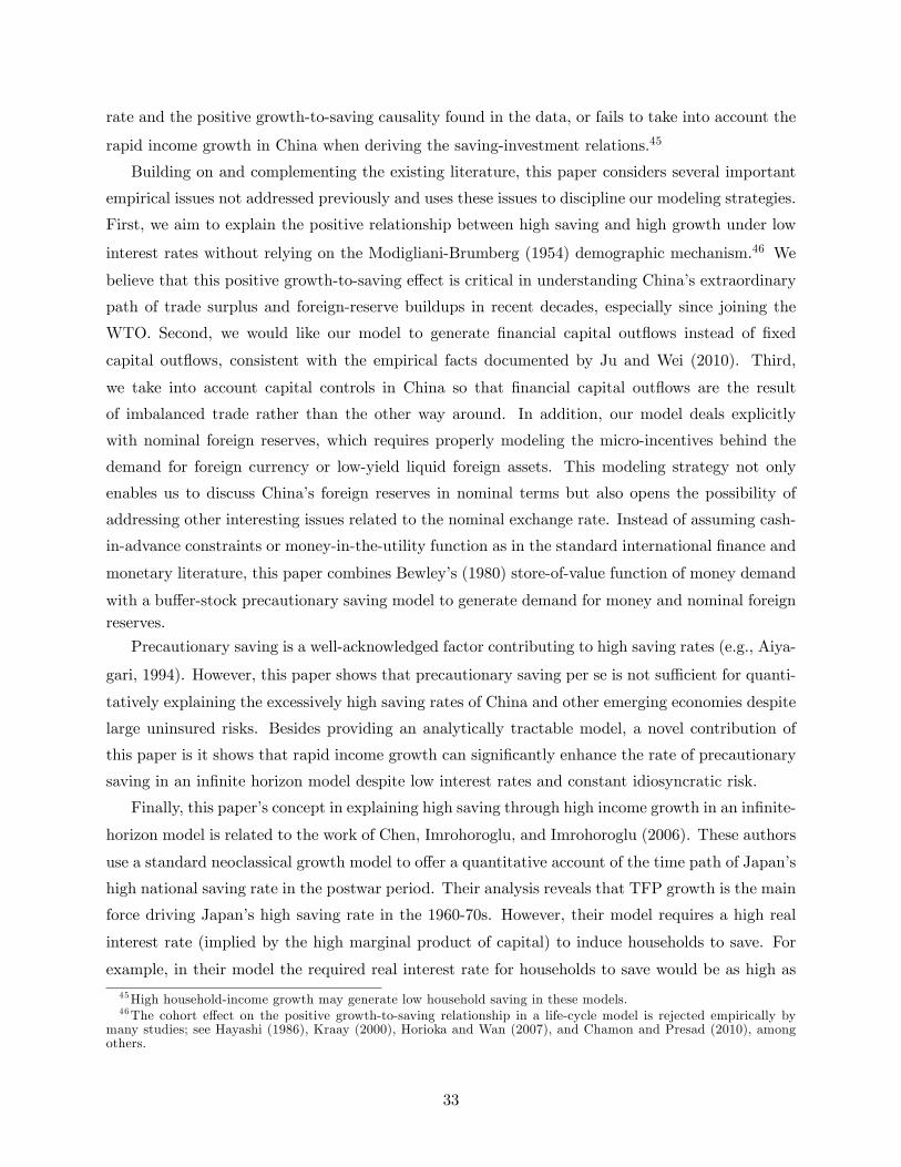
rate and the positive growth-to-saving causality found in the data, or fails to take into account the

rapid income growth in China when deriving the saving-investment relations.45

Building on and complementing the existing literature, this paper considers several important

empirical issues not addressed previously and uses these issues to discipline our modeling strategies.

First, we aim to explain the positive relationship between high saving and high growth under low

interest rates without relying on the Modigliani-Brumberg (1954) demographic mechanism.46 We

believe that this positive growth-to-saving e¤ect is critical in understanding China�s extraordinary

path of trade surplus and foreign-reserve buildups in recent decades, especially since joining the

WTO. Second, we would like our model to generate �nancial capital out�ows instead of �xed

capital out�ows, consistent with the empirical facts documented by Ju and Wei (2010). Third,

we take into account capital controls in China so that �nancial capital out�ows are the result

of imbalanced trade rather than the other way around. In addition, our model deals explicitly

with nominal foreign reserves, which requires properly modeling the micro-incentives behind the

demand for foreign currency or low-yield liquid foreign assets. This modeling strategy not only

enables us to discuss China�s foreign reserves in nominal terms but also opens the possibility of

addressing other interesting issues related to the nominal exchange rate. Instead of assuming cash-

in-advance constraints or money-in-the-utility function as in the standard international �nance and

monetary literature, this paper combines Bewley�s (1980) store-of-value function of money demand

with a bu¤er-stock precautionary saving model to generate demand for money and nominal foreignreserves.

Precautionary saving is a well-acknowledged factor contributing to high saving rates (e.g., Aiya-

gari, 1994). However, this paper shows that precautionary saving per se is not su¢ cient for quanti-

tatively explaining the excessively high saving rates of China and other emerging economies despite

large uninsured risks. Besides providing an analytically tractable model, a novel contribution of

this paper is it shows that rapid income growth can signi�cantly enhance the rate of precautionary

saving in an in�nite horizon model despite low interest rates and constant idiosyncratic risk.

Finally, this paper�s concept in explaining high saving through high income growth in an in�nite-

horizon model is related to the work of Chen, Imrohoroglu, and Imrohoroglu (2006). These authors

use a standard neoclassical growth model to o¤er a quantitative account of the time path of Japan�s

high national saving rate in the postwar period. Their analysis reveals that TFP growth is the main

force driving Japan�s high saving rate in the 1960-70s. However, their model requires a high real

interest rate (implied by the high marginal product of capital) to induce households to save. For

example, in their model the required real interest rate for households to save would be as high as

45High household-income growth may generate low household saving in these models.46The cohort e¤ect on the positive growth-to-saving relationship in a life-cycle model is rejected empirically by

many studies; see Hayashi (1986), Kraay (2000), Horioka and Wan (2007), and Chamon and Presad (2010), amongothers.

33

14 percent a year when the TFP growth rate is 10% per year and the time discounting factor is

0.96. But a real interest rate this high is rarely observed in Japanese or Chinese data (see an earlier

version of this paper (Wen, 2009a) for more discussions on this issue and the relevant data). In

contrast, our model can generate a high saving rate in a zero or even negative real interest rate

environment, which is consistent with the real-life scenario in China.47

8 Conclusion and Remarks for Future Research

This paper provides a simple, analytically tractable framework to understand China�s massive trade

imbalances and foreign-reserve buildups. Despite its simplicity, the model performs quite well in

qualitatively and quantitatively explaining the Chinese data. Our framework is disciplined by two

sets of important empirical facts: (i) China has a high income growth rate and a depressed (negative)

real interest rate, and (ii) China has capital controls and its large �nancial capital out�ow is the

consequence rather than the source of its current account surplus. These facts were the motivation

to (i) start with a trade model (that explicitly includes an export sector) and (ii) enrich the model

with the demand for low-yield liquid assets in a heterogeneous-agent framework with borrowing

constraints and uninsured risks.

Our analysis shows that China�s gargantuan foreign reserves can be a natural consequence

of rapid economic growth in conjunction with an ine¢ cient �nancial system (or lack of timely

�nancial reform) that has hampered Chinese entrepreneurs from consuming their rapidly growing

future income. Speci�cally, because of large uninsured risks and severe borrowing constraints, the

saving rate remains an increasing function of income growth even at relatively high growth rates.

Given the high growth rate of income, Chinese entrepreneurs (exporters) opt to save a substantial

fraction (more than a quarter) of their income earned from trade, which leads to the massive buildup

of China�s foreign reserves. Hence, China�s trade imbalance puzzle is resolved without appealing

to a hypothetically distorted exchange rate.48

The fundamental determinants of the exchange rate include not only excess demand for tradable

47See Appendix B for a model with capital investment that shows that a high national saving rate and investmentrate can be generated from high TFP growth despite a negative real interest rate.48Even a layman can understand the following arithmetic: Suppose the real exchange rate between Chinese goods

and American goods is 1:1� for example, 1 Chinese orange for 1 American apple. Whenever China gives up Noranges, it receives N American apples in return. Trade is therefore always balanced between the two countriesbecause the total value of Chinese exports (N oranges) always equals the value of imports (N apples). Suppose theChinese government is able to manipulate the real exchange rate so that Chinese workers must give up 100 oranges for1 American apple. Despite the extremely cheap Chinese products with a real exchange rate of 100:1, trade betweenthe two nations is still balanced� for every 100 oranges China exports to the U.S., it receives 1 U.S. apple, so thetotal value of Chinese exports (100�N oranges) still equals the total value of Chinese imports (N American apples).Therefore, trade can always be balanced regardless of the exchange rate. However, imbalanced trade could occur inthe following situation: Suppose Chinese workers gave up 100 oranges and received 1 U.S. dollar as payment, withwhich they could buy 1 American apple. But instead of spending the entire dollar on American apples, Chineseworkers bought only half an American apple and kept the remaining 50c/ as savings. In this case, China would incura trade surplus of 0:5 American apple, equivalent to lending 50 oranges to American consumers by holding 50c/ asIOUs. The question is why Chinese workers opt to do that? This question is answered in this paper.

34

goods but also excess demand for tradable assets.49 Even though the home country in our model

runs a massive current account surplus, the supply of dollars in the local exchange market (P �t Yt)

always equals the total demand of dollars (P �t Ct +Mt+1 �Mt) in our model. Hence, there is no

pressure for the home currency to appreciate. Therefore, trade imbalances between China and the

rest of the world need not be attributed to a linked exchange rate or a undervalued home currency.

This conclusion holds true even if entrepreneurs in our model do not want to use dollars as a

saving device because they can always opt to exchange the amount (Mt+1 �Mt) in each period

with their government for home currency. In this case, the government would become the holder of

foreign reserves without a¤ecting our results. Also, the government should have no fear of in�ation

even without sterilization because households will save, instead of spend, the home currency they

exchanged with the government.50

Some important issues about China�s patterns of trade and reserve buildups remain untouched

by this paper. First, this paper focuses on the source of China�s foreign reserves but does not

explicitly explain the optimal portfolio aspect of the reserves. Currently, the bulk of China�s for-

eign reserves are in U.S. government bonds. Why does the Chinese government not diversify its

portfolio better by investing in high-yield assets? It is noteworthy that foreign reserves held by the

government are owned by the private sectors since they stem from the private sectors�precaution-

ary savings but are bought (borrowed) by the government through sterilization.51 Therefore, the

government is e¤ectively holding the reserves on behalf of the private sectors and must stand ready

whenever the private sectors want to buy back the dollars sold to the government. This implies

that the reserves must be predominantly in the form of liquid assets.

Second, China does not necessarily incur a trade surplus with all of its major trading partners.

For example, in sharp contrast to the case of Sino-U.S. trade, China has been running large trade

de�cits with Japan and South Korea in the past decade (see, e.g., Dekle, Eaton, and Kortum, 2007

and 2008). This is puzzling from the viewpoint of the global imbalance literature (e.g., Mendoza

et al. 2009) because Japan and Korea both have a far more advanced �nancial system than China,

yet China is not lending goods or having net capital out�ows to these major trading partners

despite its rapidly growing trading volumes with them. A noteworthy point is that for every dollar

49This simple point is often ignored by trade theories and by a large body of the existing literature arguing for theappreciation of the RMB (see, e.g., Evenett, 2010; and Krugman, 2010).50Our analysis suggests that gradual �nancial development in China will ultimately reduce household saving rate

and eliminate China�s trade imbalances with the developed world. Recent household data suggest that this mechanismmay be already taking e¤ect.51The Chinese government buys dollars from residents by issuing bonds to retrieve the local currency. This practice

(sterilization) enables the government to absorb dollars without increasing the supply of local currency when tradesurplus increases. O¢ cially, the government is also obligated to buy dollars from the private sector to maintain a�xed exchange rate. Thus, sterilization is equivalent (in outcome) to a situation where the Chinese government meetsthe savings demands of its domestic residents by selling them Chinese government bonds and using the proceedsto purchase foreign (especially U.S.) bonds. If the private sectors want to increase spending on foreign goods, inprinciple they can exchange dollars back from the government by selling bonds. In this sense, the Chinese governmentis functioning like a bank, enabling savers to deposit and invest their foreign income.

35

Chinese exporters make in trading with the U.S., only one fourth is saved; the remaining 75c/ is

not spent entirely on U.S. goods because Chinese entrepreneurs also need dollars to import raw

materials and intermediate goods from other countries to produce �nal consumption goods. Japan

and South Korea are the major suppliers of China�s intermediate goods and assembly parts. As

a result, Japan and South Korea have successfully transformed themselves from America�s �nal-

goods suppliers into China�s intermediate-goods suppliers through a Heckscher-Ohlin-Ricardian

mechanism of comparative advantage: They ship intermediate goods and assembly parts to China

and re-export them to the U.S. in the form of �nal goods. This roundabout export process can

signi�cantly reduce labor and raw material costs.52 Therefore, theories of both international trade

(that deal with excess demand of tradable goods) and international �nance (that deal with excess

demand of tradable assets) must be combined to fully understand the patterns of the imbalanced

world trade. Hopefully, extending the simple incomplete-market model developed in this paper to a

multi-country general-equilibrium framework with tradable intermediate goods and assets, as well

as di¤erentiated labor costs will explain the pattern of trade among the U.S., China, and China�s

Asian trading partners (such as Japan, Korea, and Taiwan). Explicitly dealing with these issues is

beyond the scope of this paper, so they are left to future research.

52According to Gaulier, Lemoine, and Ünal-Kesenci (2007), "Assembly and processing of imported inputs for re-export account for about half of China�s foreign trade. These activities have been the most dynamic part of China�sexports since the early 1990s and have allowed for their rapid diversi�cation from textile to electronics. Assemblyand processing is responsible for China�s entire trade surplus with the US and Europe."

36

References

[1] Aiyagari, R., 1994, Uninsured idiosyncratic risk and aggregate saving, Quarterly Journal of

Economics 109(3), 659-684.

[2] Benjamin, D., L. Brandt, and J. Giles, 2006, Inequality and Growth in Rural China: Does

Higher Inequality Impede Growth? Working Paper IZA DP No. 2344.

[3] Bernard, Andrew B., Jonathan Eaton, J. Bradford Jensen, and Samuel Kortum, 2003, Plants

and Productivity in International Trade, American Economic Review 93, 1268-1290.

[4] Bewley, T., 1980, The optimum quantity of money, in Kareken, J., and Wallace, N., eds.,

Models of Monetary Economics. Minneapolis, MN: Federal Reserve Bank of Minneapolis, 1980,

169-210.

[5] Brandt, Loren, Johannes Van Biesebroeck, and Yifan Zhang, 2009, Creative Accounting or

Creative Destruction? Firm-Level Productivity Growth in Chinese Manufacturing, NBER

Working Paper 15152.

[6] Buera, F. and Y. Shin, 2010, Productivity growth and capital �ows: The dynamics of reform,

Working Paper, Washington University in St. Louis.

[7] Caballero, Ricardo, Emmanuel Farhi, and Pierre-Olivier Gourinchas, 2008, An equilibrium

model of global imbalances and low interest rates, American Economic Review 98(1), 358-

393.

[8] Carroll, C and D. Weil, 1994, Saving and Growth: A Reinterpretation, Carnegie-Rochester

Conference Series on Public Policy 40, 133-192.

[9] Carroll, C. and O. Jeanne, 2009, A tractable model of precautionary reserves, net foreign

assets, or sovereign wealth funds, Peterson Institute for International Economics Working

Paper Series WP 09-10.

[10] Chamon, M. and E. Prasad, 2010, Why are saving rates of urban households in China rising?

American Economic Journal: Macroeconomics 2(1), 93-130.

[11] Chamon, M., K. Liu, and E. Prasad, 2010, Income Uncertainty and Household Savings in

China, NBER and IZA Discussion Paper No. 5331.

[12] Chaney, T., 2008, Distorted gravity: Heterogeneous �rms, market structure, and the geography

of international trade, American Economic Review 98, 1707-1721.

37

[13] Chang, Y. and S. Kim, 2006, From Individual to aggregate labor supply: A quantitative

analysis based on a heterogeneous agent macroeconomy, International Economic Review 47(1),

1�27.

[14] Chen, K., A. Imrohoroglu, and S. Imrohoroglu, 2006, The Japanese saving rate, American

Economic Review 96(5), 1850-1858.

[15] China Statistical Year Book (2008, 2009).

[16] Deardor¤, Alan, 2010, A trade theorist�s take on global imbalance, in Evenett, Simon J. (ed.),

The US-Sino Currency Dispute: New Insights from Economics, Politics and Law. London:

VoxEU.Org Publications, Centre for Economic Policy Research, 43-47.

[17] DeBacker, J., B. Heim, V. Panousi, and I. Vidangos, 2010, Rising Inequality: Transitory or

Permanent? New Evidence from a Panel of U.S. Tax Returns 1987-2006, Working Paper.

[18] Dekle, Robert, Jonathan Eaton, Samuel Kortum, 2007, Unbalanced trade, American Economic

Review: Papers and Proceedings 97, 351-355.

[19] Dekle, Robert, Jonathan Eaton, Samuel Kortum, 2008, Global rebalancing with gravity: Mea-

suring the burden of adjustment, IMF Stu¤ Papers 55(3), 511-540.

[20] Eaton, Jonathan and Kortum, Samuel, 2002, Technology, Geography, and Trade, Econometrica

70(5), 1741-1780.

[21] Evenett, Simon J. (ed.), 2010, The US-Sino Currency Dispute: New Insights from Economics,

Politics and Law. London: VoxEU.Org Publications, Centre for Economic Policy Research.

[22] Flannery, Russell, 2009, China�s 400 Richest, Forbes.com, November 4, 2009;

http://www.forbes.com/2009/11/04/china-richest-billionaires-bu¤ett-baidu-china-

billionaires-09-wealth_intro.html.

[23] Friedman, M., 1957, A Theory of the Consumption Function. Princeton, NJ: Princeton Uni-

versity Press.

[24] Gaulier, Guillaume, Françpise Lemoine, and Deniz Ümal-Kesemci, 2007, China�s emergence

and the reorganization of trade �ows in Asia, China Economic Review, 18(3), 209-243.

[25] Ghironi, F. and M. Melitz, 2005. International Trade and Macroeconomic Dynamics with

Heterogeneous Firms, Quarterly Journal of Economics, 120(3), 865-915.

38

[26] Gottschalk, P. and R. Mo¢ tt, 1994, The growth of earnings instability in the U.S. labor

market, Brookings Papers on Economic Activity, 217-272.

[27] Gottschalk, P. and R. Mo¢ tt, 2009, The rising instability of U.S. earnings, Journal of Economic

Perspectives 23, 3-24.

[28] Haider, S., 2001, Earnings instability and earnings inequality of males in the United State,

1967-1991, Journal of Labor Economics 19, 799-836.

[29] Hayashi, F., 1986, Why Is Japan�s Saving Rate So Apparently High? NBER Macroeconomics

Annual 1, 147-210.

[30] Heathcote, J., K. Storesletten, and G. Violante, 2009, Consumption and Labor Supply with

Partial Insurance: An Analytical Framework, Federal Reserve Bank of Minneapolis Research

Department Sta¤ Report 432.

[31] Horioka, C. Y. and J. Wan, 2007, The Determinants of Household Saving in China: A Dynamic

Panel Analysis of Provincial Data, Journal of Money, Credit, and Banking 39(8), 2077�2096.

[32] Ishikawa, T. and K. Ueda, 1984, The bonus payment system and Japanese personal savings,

in M. Aoki, ed., The Economic Analysis of the Japanese Firm. Amsterdam: North Holland,

133-192.

[33] Jin, Keyu, 2011, Credit Constraints and Growth in a Global Economy, Working Paper, London

School of Economics.

[34] Ju, Jiandong and Shang-Jin Wei, 2010, Domestic institutions and the bypass e¤ect of �nancial

globalization, NBER Working Paper 13148.

[35] Kraay, Aart, 2000, Household Saving in China, World Bank Economic Review 14(3), 545-570.

[36] Krugman, Paul, 2010, Taking on China, New York Times, 15 March 2010.

[37] Lagos, R. and R.Wright, 2005, A Uni�ed Framework for Monetary Theory and Policy Analysis,

Journal of Political Economy 113(3), 463-484.

[38] Liu, Yuanli, Keqin Rao, and William C. Hsiao, 2003, Medical Expenditure and Rural Impov-

erishment in China, Journal of Health, Population, and Nutrition 21(3), 216-222.

[39] Lu, D., 2010, Exceptional exporter performance? Evidence from Chinese manufacturing �rms,

Working Paper, University of Chicago.

39

[40] Lucas, R.E. Jr., 1980, Equilibrium in a pure currency economy, Economic Inquiry 18(2), 203-

220.

[41] Mark, A. and G. Gopinath, 2007, Emerging market business cycles: The cycle is the trend,

Journal of Political Economy 115(1), 69-102.

[42] Melitz, Marc, 2003, �The Impact of Trade on Intra-Industry Reallocations and Aggregate

Industry Productivity, Econometrica 71, 1695-1725.

[43] Mendoza, Enrique G., Vincenzo Quadrini, and José-Victor Rios-Rull, 2009, Financial integra-

tion, �nancial development, and global imbalances, Journal of Political Economy 117, 371-416.

[44] Modigliani, F., 1970, The life-cycle hypothesis of saving and intercountry di¤erences in the

saving ratio, in "Induction, Growth, and Trade: Essays in Honour of Sir Roy Harrod" (Oxford:

Clarendon Press) 197-225.

[45] Modigliani, F. and R. Brumberg, 1954, Utility analysis and the consumption function: An

attempt at integration, in Post-Keynesian Economics. Kenneth Kurihara, ed.

[46] Modigliani, Franco and Richard H. Brumberg, 1954, Utility Analysis and the Consumption

Function: An Interpretation of Cross-Section Data, in Kenneth K. Kurihara, ed.: Post-

Keynesian Economics. New Brunswick, NJ: Rutgers University Press, pp 388-436.

[47] Modigliani, F. and S. Cao, 2004, The Chinese saving puzzle and the life-cycle hypothesis,

Journal of Economic Literature 42(1), 145-170.

[48] Mo¢ tt, R. and P. Gottschhalk, 1995, Trends in the covariance structure of earnings in the

US.: 1969-1987, Working Paper.

[49] Mo¢ tt, R. and P. Gottschhalk, 2008, Trends in the transitory variance of male earnings in the

U.S.: 1970-2004, Working Paper.

[50] Platt, Kevin Holden, 2007, Chinese Air Pollution Deadliest in World, National Geographic

News, July 9, 2007.

[51] Ricardo, D., 1817, On the Principles of Political Economy and Taxation, P. Sra¤a, ed., Cam-

bridge, Cambridge University Press, 1951.

[52] Sabelhaus, J. and J. Song, 2009, Earnings volatility across groups and time, Working Paper.

[53] Shin, D. and G. Solon, 2008, Trends in Men�s earnings volatility: What does the panel study

of income dynamics show? NBER Working Paper 14075.

40

[54] Sandri, Damiano, 2010, Growth and capital �ows with risky entrepreneurship, IMF Working

Paper WP/10/36.

[55] Solis, Hilda L. and Joseph A. Main, 2011, Injury Experience in Coal Mining, 2009, U.S.

Department of Labor, IR 1348, 2011.

[56] Song, Z., K. Storesletten, and F. Zilibotti, 2011, Growing like China, American Economic

Review 101, 202-241.

[57] Song, Z. and D.T. Yang, 2011, Life Cycle Earnings and the Household Saving Puzzle in a

Fast-Growing Economy, Working Paper.

[58] Wang, X. and Y. Wen, 2011, Can rising housing prices explain China�s high household saving

rate? Federal Reserve Bank of St. Louis Review 93(2), 67-88.

[59] Wang, Hong-Ming, 2009, Present Situation of Road Tra¢ c Accident in China and Its Charac-

teristics, China Safety Science Journal 19(10), 121-126.

[60] Wang, H., T. Xu and J. Xu, 2007, Factors Contributing to High Costs and Inequality in China�s

Health Care System, Journal of the American Medical Association 298(16), 1928-1930.

[61] Wang, O., 2011, An empirical analysis of rural household income distribution, (in Chinese),

working paper.

[62] Wei, S.-J. and X. Zhang, 2011, The competitive saving motive: Evidence from rising sex ratios

and savings rates in China, Journal of Political Economy, 119(3), 551-564.

[63] Wen, Yi, 2009a, Saving and growth under borrowing constraints: Explaining the high saving

rate puzzle, Federal Reserve Bank of St. Louis Working Paper 2009-045C.

[64] Wen, Yi, 2009b, Liquidity and welfare in a heterogeneous-agent economy, Federal Reserve

Bank of St. Louis Working Paper 2009-019B.

[65] Wen, Yi, 2011, Making sense of China�s excessive foreign reserves, Federal Reserve Bank of St.

Louis Working Paper 2011-006A.

[66] Xing, J.J., W.D. Liu, X.J. Sun, J.W. Zhang, 1996, Fatigue and accidencts of underground coal

miners in China, China Safety Science Journal 6(5), 31-34.

[67] Xu, Ling, Yan Wang, Charles D. Collins, and Shenglan Tang, 2007, Urban health insurance

reform and coverage in China using data from National Health Services Surveys in 1998 and

2003, BMC Health Services Research 2007, 7-37.

41

Appendix A

I. Proof of Proposition 1.

Proof. Denote x � 11+�m(i) + wN(i) as cash in hand net of bonus income, and f�t(i); �t(i)g

as the Lagrangian multipliers associated with equations (4) and (5), respectively. The �rst-order

conditions for fct(i); Nt(i);mt+1(i)g are given, respectively, by

�t(i)

ct(i)= �t(i) (28)

a = wt

Z�t(i)dF (�) (29)

(1 + �g)�t(i) =�

1 + �Et

Z�t+1(i)dF (�) + �t(i) =

�

(1 + �)Eta

w0+ �(i); (30)

where equation (29) re�ects the fact that the labor supply must be determined before the realization

of �t(i) and vt(i) in each period. The optimal decision rules are characterized by a cuto¤ strategy.

There exist two cuto¤s f��1; ��2g for preference shocks because income shock vt(i) takes two possiblevalues. In anticipation that the cuto¤s are independent of i, consider two possible cases as follow:

Case A. m0(i) � 0, �(i) = 0. In this case, the urge to consume is low, or the income shock ishigh, or both. It is then optimal to save to prevent possible borrowing constraints in the future

when the urge to consume may be high or income may be low. Equation (30) then implies that the

shadow value of good

�(i) =�

(1 + �g) (1 + �)Et

a

wt+1� ��t: (31)

Equation (28) then implies that ct(i) = �(i)���1. The household budget constraint then implies

(1 + �g)m0(i) = x(i) + v(i)w � �(i)���1t . The requirement m0(i) � 0 then implies

�(i) � [x(i) + v(i)w] ��t � ��; (32)

which de�nes the cuto¤ ��t . However, there are two sub-cases to consider.

Case A1 : vt(i) = ��. In this sub-case the cuto¤ is given by

��1 � [x(i)� �w] ��t; (33)

and this sub-case happens with probability 1� p.Case A2 : vt(i) = �. In this sub-case the cuto¤ is given by

��2 � [x(i) + �w] ��t (34)

42

and this sub-case happens with probability p. Because xt is determined before the realization of

vt(i), it is hence independent of vt(i). Equations (33) and (34) then together imply

��2t = ��1t + 2�wt

��t > ��1: (35)

This implies that the agent adopts a lower cuto¤ for preference shocks when income is low and a

higher cuto¤ when income is high.

Case B. �(i) > 0 and m0(i) = 0. In this case, the urge to consume is high, or income is low,

or both. It is then optimal not to save. By the household budget constraint, we have c(i) =

x(i) + v(i)w. There are again two sub-cases.

Case B1 : vt(i) = ��, equation (33) then implies c(i) = ��1���1t .

Case B2 : v(i) = �, equation (34) then implies c(i) = ��2���1t . Equation (28) then implies that

�t(i) =

(�(i)��1��t if v(i) = ��

�(i)��2��t: if v(i) = �

: (36)

Clearly, if �(i) > ��1, equation (30) implies �(i) = (1 + g) ��h�(i)��1� 1i> 0; and if �(i) > ��2, equation

(30) implies �(i) = (1 + g) ��h�(i)��2� 1i> 0. In either case, m0(i) = 0.

The above analyses imply that �t(i) takes three possible values as shown in equations (31) and

(36), depending on the joint realizations of �t(i) and vt(i) in period t. Hence, the expected value,R�t(i)dF (�), can be expressed analytically. That is, equation (29) implies

1

w=

��

(1 + �g) (1 + �)E1

w0

�R(��); (37)

where R(��) � (1� p)hR����1

dF (�) +R�<��1

���1dF (��)

i+ p

hR����2

dF (�) +R�<��2

���2dF (��)

i. As a

result, the optimal cuto¤s, f��1t; ��2tg, are determined jointly by equations (37) and (35). Equation(37) implies that the cuto¤s are independent of i because �(i) and v(i) are both i.i.d. Hence,

equations (33) and (34) in turn imply that the optimal cash in hand (xt) is also independent of i

and can be written either as xt = ���1t �

�1t + �wt or as xt = ��

�1t �

�2t � �wt. Given the values of �(i),

the decision rules of consumption are given by �(i)�(i) and the decision rules of saving are given by

(1 + g)m0(i) = x� c(i).

II. Proof of Proposition 2.

43

Proof. In the steady state, the aggregate variables satisfy m0 = m;x� �w = ��1wR, and x+ �w =��2wR. So equation (16) can be rewritten as

(1 + g)m = [(1� p) ��1H1 + p��2H2]wR: (38)

Since wN = x� 11+�m

0 = ��1wR+ �w, the disposable income can be written as

} = ��1wR+ 2p�w �1

(1 + g) (1 + �)[(1� p) ��1H1 + p��2H2]wR: (39)

Hence, the saving rate is given by

� � gm

}=

g [(1� p) ��1H1 + p��2H2](1 + g) (��1 + 2p�R

�1)� 1(1+�) [(1� p) �

�1H1 + p�

�2H2]

: (40)

Since 2�R�1 = ��2 � ��1, the saving rate can be rewritten as equation (19).

III. Proof of Proposition 3.

Proof. Denoting �H(g) � [(1� p) ��1H1 + p��2H2] and G(g) ����1 + 2p�R

�1� = (1� p) ��1 + p��2.

Di¤erentiating the saving rate with respect to �g gives

d�

d�g=

��H + g @

�H@g

� h(1 + �g)G� 1

1+��Hi� g �H

hG+ (1 + g) @G@g �

11+�

@ �H@g

ih(1 + �g)G� 1

1+��Hi2 (41)

=(1 + �g)G

��H + g @

�H@g

���G+ (1 + g) @G@g

�g �H + 1

1+�g�H @ �H@g �

11+�

�H��H + g @

�H@g

�h(1 + �g)G� 1

1+��Hi2

=(1 + �g) g

hG@ �H@g �

@G@g�Hi+ (1 + g)G �H � gG �H + 1

1+��Hhg @

�H@g � �H � g @ �H@g

ih(1 + �g)G� 1

1+��Hi2

=(1 + �g) g

hG@ �H@g �

@G@g�Hi+ �H

�G� 1

1+��H�

h(1 + �g)G� 1

1+��Hi2 :

Notice that G = (1� p) ��1 + p��2 > �H = [(1� p) ��1H1 + p��2H2] because the marginal propensity

to save Hj < 1. Thus the second term in the numerator �H�G� 1

1+��H�> 0. However, the �rst

term in the numerator,hG@ �H@g �

@G@g�Hi, is negative because ��jHj decreases more than Hj when g

44

increases. This implies that d�d�g > 0 if �g = 0 andd�d�g < 0 if �g ! 1. Continuity implies there exists

a threshold �g� 2 (0;1) that renders d�d�g = 0 when �g = �g�. So it must be true that d�d�g > 0 if �g < �g

�

and d�d�g < 0 if �g > �g

�.

IV. Proof of Proposition 4.

Proof. When � = 0, there exists a unique cuto¤ ��. So equations (11) and (12) imply that the

optimal cash in hand is given by ��wR(��) = x � m(i) + wN(i). Using the saving decision rule

in equation (10), the condition that N(i) > 0 then implies (1 + �g) ��wR(��) > (1 + �g)m(i) =

wR(��)max f�� � �(i); 0g. Since the maximum value of max f�� � �(i); 0g is �� � 1 (recall thesupport of �(i) 2 [1;1]), the above inequality is satis�ed if

(1 + �g) ��R(��) > R(��) [�� � 1] , (42)

which is clearly true for any parameter values in the model. Hence, regardless of the realization

of preference shocks, the labor supply of each entrepreneur is strictly positive. On the other hand,

the condition that N(i) < �N implies (1 + �g) ��wR(��) < max f�� � �(i); 0g+ w �N . This inequalitycan be ensured if the function max f�� � �(i); 0g takes the smallest value, which is 0. Hence, theabove inequality is satis�ed as long as

(1 + �g) ��R(��) < �N: (43)

Based on equation (12), the above inequality is equivalent to the condition (1+�g)2

� �� < �N . Under

Pareto distribution, we have R(��) = 1 + 1��1�

���, so the cuto¤ can be solved in closed-form as

�� =h(� � 1)

�1+�g� � 1

�i� 1�and the above inequality becomes

(1 + �g)2

�

�(� � 1)

�1 + �g

�� 1��� 1

�

< �N: (44)

Given that � > 1, the LHS of the above inequality is increasing in �g. Since there exists a maximum

value of the growth rate �gmax =����1 � 1 such that if �g � �gmax, we have �� = 1 and m(i) = 0 for

all i, and in this case wN(i) = c(i) and N(i) = a. Therefore, hours worked by each entrepreneur is

strictly bounded above by a �xed number �N = (1+�gmax)2

� = ��

���1

�2for �g < �gmax or by the �xed

number �N = a for �g � �gmax.

V. Proof of Proposition 5.

45

Proof. When technology At is stochastic and follows the law of motion in equation (23), the

general equilibrium path of the rescaled benchmark model can be characterized by the set of

variables, fct;mt+1; ��t ; xt; Nt; g, which can be solved uniquely by the following system of equations:

ct = (1� p)D(��1t) (xt � �wt) + pD(��2t) (xt + �wt) (45)

(1 + gt)mt+1 = (1� p)H(��1t) (xt � �wt) + pH(��2t) (xt + �wt) (46)

1 + gtwt

= �Et1

wt+1R(��1t) (47)

xt � mt + wtNt + (2p� 1) �wt = ��1tR(��1t)wt + �wt; (48)

plus equation (24) and standard transversality conditions.

In general equilibrium, wt = 1+gt. So equation (47) becomes 1 = �R(��1t)Et1

1+gt+1, which solves

implicitly for the cuto¤ ��t and the cuto¤ ��2t = �

�1t + 2�R

�1(��1t). Given the cuto¤s, equations (45)

and (48) solve for the optimal consumption path as

ct = [(1� p)D(��1t)��1tR(��1t) + pD(��2t)��2tR(��1t)] (1 + gt) ; (49)

and equations (46) and (48) solve for the optimal foreign reserves as

(1 + gt)mt+1 = [(1� p)H(��1t)��1tR(��1t) + pH(��2t)��2tR(��1t)] (1 + gt) : (50)

When p = 12 , equation (48) implies wtNt = �

�1tR(�

�1t)wt+�wt�mt, which in turn implies employment

in the tradable sector:

Nt = ��1tR(�

�1t) + ��

mt

(1 + gt)= ��1tR(�

�1t) + ��

1

2

H(��1t�1)��1t�1R(�

�1t�1) +H(�

�2t�1)�

�2t�1R(�

�2t�1)

(1 + gt):

(51)

Therefore, year-to-year changes in foreign reserves in period t are given by

(1 + gt)mt+1 �mt = yt

�1� ct

(1 + gt)Nt

�(52)

= yt

"1�

12 [(1� p)D(�

�1t)�

�1tR(�

�1t) + pD(�

�2t)�

�2tR(�

�1t)]

��1tR(��1t) + � � 1

2(1+gt)

�H(��1t�1)�

�1t�1R(�

�1t�1) +H(�

�2t�1)�

�2t�1R(�

�2t�1)

�# :Multiplying the lowercase variables on both sides of the above equation by At�1 gives equation

(25).

46

Using the law of motion in equation (23) and assuming lognormal distribution for "t with mean

zero and variance �2", equation (47) implies

1 = �R(��1t)Et1

1 + gt+1= �R(��1t)

�1 + �g

1 + gt

��g e 12�2"1 + �g

: (53)

With � following the Pareto distribution F = 1 � ���, we have R(��1t) = (1� p)h1 + 1

��1����1t

i+

ph1 + 1

��1����2t

i, so the above equation solves for the cuto¤s f��1t; ��2tg in conjunction with equation

(13).

47

Appendix B (Not for Publication)

The benchmark model does not have capital. Therefore, that model cannot directly answer the

broader question of why China�s high investment rate is unable to completely absorb its domestic

savings. Also, the benchmark model does not have nontradable goods. This appendix extends the

benchmark model to a more general setting with capital and a nontradable-goods sector.

There are two production sectors in the home country� a domestic sector (sector 1) that pro-

duces nontradable goods and an export sector (sector 2) that produces tradable goods. Because

of capital controls and an inconvertible home currency, residents of the home country cannot use

foreign currency earned from the export sector to purchase domestic goods and assets, nor can

they use income earned from the nontradable-goods sector to buy foreign goods and assets. In

other words, nontradable goods are purchased by home currency (RMB) and tradable goods are

purchased by foreign currency (USD). However, households in country H can bypass the capital

controls through working in both nontradable and tradable sectors. Therefore, despite the cap-

ital control, households are able to adjust their baskets of consumption goods for tradable and

nontradable goods by choosing an optimal mixture of hours worked in each sector.

Also because of capital controls, �rms in the domestic sector must use income earned from

domestic sales to rent capital from a domestic rental market, while �rms in the export sector can

use foreign income to rent capital from an international market with a constant world real interest

rate �rw. Fixed capital is not mobile across sectors but labor is. This setup of segregated capital

markets not only captures the reality in China (such as large capital adjustment costs, irreversible

investment, the lack of a resale capital goods market, and so on), but also allows the model to

generate the Ballasa-Samuelson e¤ect of technology growth on the real exchange rate even though

the rate of productivity growth in both the nontradable-goods and tradable-goods sectors is the

same (see Wen, 2009a, for more discussions on the determination of the exchange rate and the

Ballasa-Samuelson e¤ect).

Technology. Sector j (j = 1; 2) has the following production technology:

Yjt = K�jt (AtNjt)

1�� ; (54)

where At denotes a country�s aggregate technology level with a stochastic growth rate speci�ed in

equation (23). The demands for capital and labor in sector j are given by

rjt + � = �YjtKjt

= �

�NjtKjt

�1��A1��t (55)

Wjt = (1� �)YjtNjt

= (1� �)�KjtNjt

��A1��t ; (56)

48

where

r2t = �rw (57)

is a constant world interest rate in the international rental market.

Labor mobility across sectors implies �1tW1t = �2tW2t, where �jt denotes the marginal utility

of income received from sector j. Hence, the real price of tradable goods in terms of nontradable

goods� the real exchange rate in the economy� is given by et � �2t�1t

= W1tW2t. Equations (55) and

(56) imply

et =

��rw + �

r1t + �

� �1��

: (58)

Hence, the real exchange rate is in�uenced by aggregate technology shocks through changes in the

domestic real interest rate. In particular, a higher productivity growth leads to a higher domestic

interest rate, which implies that nontradable goods become more expensive relative to tradable

goods, so the real exchange rate appreciates (et decreases). This captures the Ballasa-Samuelson

e¤ect in an environment with identical productivity growth across tradable and nontradable-goods

sectors.

Along a balanced growth path, the real wages fW1t;W2tg and outputs fY1t; Y2tg in both sectorsall grow at the rate of long-run productivity growth (�g) in the absence of aggregate uncertainty

("t = 0), while hours worked in both sectors are constant over time. To facilitate the analysis of

a stochastic equilibrium path under aggregate uncertainty, we rescale all variables in the model

by the level of technology At�1 except for hours worked. Using lowercase letters to denote the

transformed variables, zjt � ZjtAt�1

, the production functions become

yjt = (1 + gt)1�� k�jtN

1��jt (59)

and the real wages become

wjt = (1� �)yjtNjt

= (1� �)�kjtNjt

��(1 + gt)

1�� : (60)

Households. As in the benchmark model, there is a continuum of households in country H

indexed by i 2 [0; 1]. Each household has two members (husband and wife); one works in the

nontradable-goods sector and the other works in the tradable-goods (exporting) sector. Each

household consumes two types of goods: nontradable goods produced at home and foreign goods

produced abroad.

Households put their domestic savings in banks and earn a real gross rate of return 1 + rat .

Households exchange their foreign savings (in dollars) with the government for government bonds

49

(sterilization). For simplicity and without loss of generality, assume that government bonds yield

zero interest rate. Therefore, in the model it does not matter whether the households hold dollars

or local government bonds. As documented by Wen (2009a), �nancial repression in China leads

to a low and even negative real deposit rate for household savings. Despite this, however, the

bulk of household wealth is kept in the form of bank deposits because of underdeveloped �nancial

markets in China. On the other hand, �rms must borrow funds from monopolistic state-owned

banks at market interest rate rt. To capture this reality, we assume that the real rate of return to

household savings is zero (ra = 0), and state-owned banks earn monopoly pro�ts (rt � ra) st, whichare returned in a lump sum to households. We will show that households in both sectors still save

excessively despite the low real deposit rate, as in the benchmark model.

Let st(i) � St(i)At�1

denote the rescaled home asset and mt(i) � Mt(i)At�1P �t

the rescaled real money

balances for foreign currency held by household i. Household i�s consumption for home goods is

denoted as c1t(i) � C1t(i)At�1

, imported goods as c2t(i) � C2t(i)At�1

, and hours worked in sector j as Njt(i).

For simplicity, assume P �t = P�t�1, so the in�ation rate is zero. Household i�s problem is to solve

maxE0

1Xt=0

�t f�t(i) [ 1 log c1t(i) + 2 log c2t(i)]�N1t(i)�N2t(i)g (61)

subject to

c1t(i) + (1 + gt) st+1(i) � x1t(i) + vt(i)wt (62)

st+1(i) � 0 (63)

c2t(i) + (1 + gt)mt+1(i) � x2t(i) + vt(i)wt (64)

mt+1(i) � 0; (65)

where vt(i) denotes idiosyncratic income shocks, x1t(i) is net wealth (cash in hand) in terms of

income earned in sector 1:

x1t(i) � w1tN1t(i) + st(i) + �t; (66)

and x2t(i) is cash in hand in sector 2:

x2t(i) � w2tN2t(i) +mt(i); (67)

where �t = r1tRst(i)di denotes average pro�t income distributed from domestic banks. The

parameter j in the preference controls the relative equilibrium size of the domestic and export

sectors.

Equation (62) is the budget constraint pertaining to domestic income, which state that total

real wage income earned from the nontradable-goods sector can be used to �nance consumption

50

of nontradable goods (c1t) and the accumulation of home assets ((1 + g) s0 � s) subject to theborrowing constraint (63). Analogously, equation (64) denotes the budget constraints pertaining to

foreign income, which states that total real wage income earned from working in the tradable-goods

sector can be used to �nance purchases of foreign produced goods (c2t) and the accumulation of

foreign currency (real foreign reserves, (1 + g)m0 �mt) subject to the borrowing constraint (65).

For simplicity, we have assumed that income shocks (vt(i)) are symmetric across the two sectors

with distribution given by equation (6).

Proposition 6 Denoting s1t � st and s2t � mt, the decision rules of consumption, savings, and

cash in hand for household i are given by

cjt(i) =

8>><>>:min

n�(i)��jl; 1o[xjt � �wjt] ; with probability 1� p

minn�(i)��jh; 1o[xjt + �wjt] ; with probability p

(68)

(1 + gt) sjt+1(i) =

8>><>>:max

n��jl��(i)��jl

; 0o[xjt � �wjt] ; with probability 1� p

maxn��jh��(i)��jh

; 0o[xjt + �wjt] ; with probability p

(69)

xjt = jwjt��jltRt + �wjt; (70)

where the cuto¤ variables ��jlt and ��jht are determined by the following equations:

1 + gtwjt

= �R(�jlt)Et1

wjt+1(71)

��jht = ��jlt + 2�R

�1jt ; (72)

where the liquidity premium function R(�) is given by Rjt � (1� p)hR�<��j

dF (�) +R����jl

���jldF (�)

i+

phR�<��jh

dF (�) +R����jh

���jhdF (�)

i.

Proof. Similar to the proof of Proposition 1.

These decision rules are similar to those in the benchmark model. However, the optimal cuto¤s

in each sector� determined by equations (71) and (72)� may di¤er across sector j because the real

wage may di¤er across sectors (because of di¤erent capital markets and real interest rates).

Denoting any aggregate variable zjt �Rzjt(i)di, market clearing for the domestic capital market

impliesRs1t(i)di = k1t. Hence, the general equilibrium path of the model can be characterized by

51

the sequences of 16 variables,�cjt; sjt+1; �

�jlt; �

�jht; xjt; wjt; yjt; Njt; j = 1; 2

1t=0, which can be solved

by the following system of 16 equations (assuming p = 0:5 so that the average bonus income in

each sector is zero, �v = (2p� 1) � = 0):

cjt = (1� p)D(��jlt) [xjt � �wjt] + pD(��jht) [xjt + �wjt] (73)

(1 + gt) sjt+1 = (1� p)H(��jlt) [xjt � �wjt] + pH(��jht) [xjt + �wjt] (74)

1 + gtwjt

= �Et1

wjt+1R(��jlt) (75)

��jht = ��jlt + 2�R

�1jt (76)

xjt = j��jltR(�

�jlt)wjt + �wjt (77)

c1t + (1 + gt) k1t+1 � (1� �) k1t = y1t (78)

c2t + (1 + gt)mt+1 �mt + (�rw + �) k2t = y2t (79)

where �rw + � = � y2tk2t , plus the four equations (59) and (60) and standard transversality conditions.

The pro�t income from �nancial intermediaries is given by

�t = (r1t � rat )Zs1t(i)di = r1tk2t: (80)

Hence, equation (78) is also the goods market-clearing condition for the nontradable-goods sector.

Equation (79) is the household�s budget constraint in the export sector, where (�rw + �) k2t is rental

payment for capital services. Thus, income from exports is used to �nance imports of consumption

goods (c2), capital rental costs ((�rw + �) k2t), and foreign-reserve accumulation (mt+1 �mt).

The model has a unique steady state. The eigenvalue method easily con�rms that the steady

state is a saddle, so the general equilibrium path implied by the above system of dynamic equations

is unique near the steady state. To see the distortion e¤ect of capital control, suppose � = 0, so

that ��jlt = ��jht in sector j = 1; 2. Equations (73) and (77) then imply

c1tc2t

=D (��1t) �

�1tR(�

�1t)

D (��2t) ��2tR(�

�2t)

1w1t 2w2t

� 't 1w1t 2w2t

; (81)

where the coe¢ cient ' 6= 1 measures e¢ ciency loss (or deadweight loss) due to capital controls.

The allocation would be e¢ cient if ' = 1.

De�ning }j as the total real disposable income in sector j, which includes wage income plus

real capital gains (i.e., interest income, if any), we have

}1t =W1tN1t +�t = X1t � St (82)

52

}2t =W2tN2t = X2t �Mt

P �t: (83)

The saving rate for each type of income in the economy is de�ned as the ratio of net changes in

asset position to disposable income in the respective sector:

�1 =St+1 � St}1t

=(1 + gt) st+1 � st

x1t � st(84)

�2 =(Mt+1 �Mt) =P

�

}1t=(1 + g)mt+1 �mt

x2t �mt: (85)

Proposition 7 Denoting �Hj � 12

�H(��jl) +H(�

�jh)�, the steady-state household saving rate in sec-

tor j is given by

� j =�g �Hj

���jlRj + �

�+ 1

2�g��H(��jh)�H(��jl)

��1 + �g � �Hj

� ���jlRj + �

�� 1

2��H(��jh)�H(��jl)

� : (86)

Proof. Similar to the proof of Proposition 2.

By rearrangement, the saving rate in equation (86) can be shown to be identical to equation

(19) in the benchmark model. So, as before, higher income growth can lead to a higher saving rate

instead of a higher propensity to consume. The national saving rate (the ratio of investment and net

exports to GDP) in the economy is given by gk+egmy1+eY2

, and the aggregate investment-to-GDP ratio

is given by gky1+ey2

. Because of trade surplus (gm > 0), the national saving rate exceeds domestic

investment rate even if the investment rate is high. For example, under the following parameter

values, � = 0:96, � = 0:1, 1 = 0:8, 2 = 0:2, � = 1:3, � = 2, and �g = 0:05, we havegk

y1+ey2= 0:4

and gk+egmy1+eY2

= 0:44. The calibrated values of f 1; 2g capture the relative sizes of the export and

the non-export sectors in China since total exports account for about 20% of GDP. The implied

national saving rate under these parameter values is 46% (not including government saving) while

the household saving rate in the tradable goods sector is gmy2 = 22%. Of the 46% national saving

rate, aggregate investment accounts for 42% of GDP and net exports accounts for 4% of GDP.

These magnitudes are consistent with Chinese data.

Appendix C (Not For Publication)

This appendix shows that the previous results do not hinge on the assumptions of capital

controls and a linked exchange rate. As in Appendix B, there are two production sectors in the

home country, one producing nontradable goods for domestic consumption and the other producing

53

tradable goods for exports. There are no capital controls and the nominal exchange rate is �exible.

The real exchange rate (the relative price of the tradable goods in terms of the nontradable goods)

is denoted by et. Households can choose to work in either sector and receive real wageWjt in sector

j = 1; 2. For simplicity and without loss of generality, there are no �xed capital and income shocks

(i.e., � = 0 and � = 0). The production technology in sector j is given by Yjt = AtF (Njt), and

the competitive real wage is given by Wjt =dYjtdNjt

. Applying the rescaling factor At�1, we have

yjt = (1 + gt)F (Njt) and wjt = (1 + gt)F 0(Njt).

Household i�s problem is to solve

maxE1Xt=0

�t f�t(i) [ 1 log c1t(i) + 2 log c2t(i)]�N1t(i)�N2t(i)g (87)

subject to

c1t(i) + etc2t(i) + (1 + gt) ~mt+1(i) � ~mt(i) + w1tN1t(i) + etw2tN2t(i) + �1t + et�2t (88)

~mt+1(i) � 0; (89)

where ~mt denotes a portfolio of assets with a real gross rate of return equal to 1, and �jt denotes

the pro�t income distributed from �rms in sector j. Because currencies are fully convertible, the

household faces only one budget constraint. The budget constraint implies that households can

combine income received from either sector to �nance consumption of both nontradable goods and

tradable goods, as well as asset accumulations.

Proposition 8 Denoting cash in hand as

xt � ~mt(i) + w1tN1t(i) + etw2tN2t(i) + �1t + et�2t; (90)

the decision rules for consumption, imports, saving, and cash in hand are given, respectively, by

c1t(i) = 1

1 + 2min

�1;�t(i)

��t

�xt (91)

etc2t(i) = 2

1 + 2min

�1;�t(i)

��t

�xt (92)

(1 + gt) ~mt+1(i) = max

���t � �(i)�(i)

; 0

�xt (93)

xt = ( 1 + 2) ��tR(�

�t )w1t; (94)

54

where the cuto¤ and real exchange rate are determined by

1 + gtw1t

= �Et1

w1t+1R(��t ) (95)

et =w1tw2t

: (96)

Proof. Similar to the proof in Proposition 1.

Equations (91)-(96) imply that

c1tc2t

= 1 2et: (97)

Compared with equation (81), lifting capital controls implies e¢ cient allocation here. However,

this e¢ ciency gain has no e¤ect on the household saving rate, as the following proposition shows.

Proposition 9 The current account surplus is given by

CAt = ( 1 + 2)�(1 + gt) �

�tR(�

�t )H(�

�t )� ��t�1R(��t�1)H(��t�1)

�; (98)

and the aggregate saving rate is given by

� t =

�(1 + gt) �

�tR(�

�t )H(�

�t )� ��t�1R(��t�1)H(��t�1)

��(1 + gt) �

�tR(�

�t )� ��t�1R(��t�1)H(��t�1)

� : (99)

Proof. Aggregating by the law of large numbers, the household decision rules (91)-(93) become

c1t = 1

1 + 2D(��t )xt (100)

etc2t = 2

1 + 2D(��t )xt (101)

(1 + gt) ~mt+1 = H(��t )xt (102)

The budget constraint becomes

c1t + etc2t + (1 + gt) ~mt+1 = ~mt + w1tN1t + etw2tN2t +�1t + et�2t: (103)

Since households own �rms, wage income plus pro�t income should equal the value of output

in each sector:

wjtNjt +�jt = yjt: (104)

Hence, market clearing in the nontradable-goods sector implies

c1t = w1tN1t +�1t: (105)

55

Equation (103) then implies

etc2t + (1 + gt) ~mt+1 = ~mt + ety2t: (106)

So the current account surplus is given by

CAt = ety2t � etc2t = (1 + gt) ~mt+1 � ~mt: (107)

Using equation (102), we have

CAt = H(��t )xt �1

1 + gt�1H(��t�1)xt�1 (108)

= ( 1 + 2)�(1 + gt) �

�tR(�

�t )H(�

�t )� ��t�1R(��t�1)H(��t�1)

�:

The aggregate saving rate is given by

� t =y1t + ety2t � [c1t + etc2t]

y1t + ety2t=

CAty1t + ety2t

; (109)

where the denominator is given by

y1t + ety2t = w1tN1t +�1t + etw2tN2t + et�2t (110)

= xt � ~mt

= xt �1

1 + gt�1H(��t�1)xt�1

= ( 1 + 2)�(1 + gt) �

�tR(�

�t )� ��t�1R(��t�1)H(��t�1)

�:

So we have equation (99).

Notice that the saving rate is precisely the same as that in equation (25) in the benchmark

model (by setting � = 0 and ��1 = ��2) and is also identical to that in the general model in Appendix

B (by setting � = 0 in the production function). Clearly, both the current account and the national

saving rate are independent of the exchange rate et. In the steady state, the current account surplus

is given by

CA = g�R(��)H(��); (111)

and the saving rate equals

� =�gH(��)

1 + �g �H(��) ; (112)

which is identical to equation (20) in the benchmark model or equation (86) in the general model

(by setting � = 0 and � = 0).

56