explaining child malnutrition in developing countries: … child... · explaining child...
TRANSCRIPT

EXPLAINING CHILD MALNUTRITION IN DEVELOPINGCOUNTRIES: A CROSS-COUNTRY ANALYSIS
Lisa C. Smith and Lawrence Haddad
FCND DISCUSSION PAPER NO. 60
Food Consumption and Nutrition Division
International Food Policy Research Institute2033 K Street, N.W.
Washington, D.C. 20006 U.S.A.(202) 862–5600
Fax: (202) 467–4439
April 1999
FCND Discussion Papers contain preliminary material and research results, and are circulated prior to a fullpeer review in order to stimulate discussion and critical comment. It is expected that most Discussion Paperswill eventually be published in some other form, and that their content may also be revised.

ABSTRACT
This paper draws on the experience of the 1970-95 period to (1) elucidate some of
the main causes of child malnutrition in developing countries; (2) undertake projections
of how many children are likely to be malnourished in the year 2020 given current trends;
and (3) identify priority actions for reducing malnutrition the most quickly in the coming
decades. The analysis is based on country fixed-effects multivariate regression using data
from 63 countries. The paper finds four "underlying" determinants to be key factors:
health environments, women's education, women's relative status, and per capita food
availability. Two "basic" determinants are also found to be important: per capita national
incomes and democracy. Due to data scarcities, the role of poverty could not be assessed.
Improvements in women's education was found to have contributed the most to past
reductions in child malnutrition. For Sub-Saharan Africa and South Asia—the regions
with the highest child malnutrition rates—the paper identifies two priority areas for future
reductions in child malnutrition: per capita food availabilities and women's education.

CONTENTS
Acknowledgments . . . . . . . . . . . . . . . . . . . . . . . . . . . . . . . . . . . . . . . . . . . . . . . . . . . . xi
1. Introduction . . . . . . . . . . . . . . . . . . . . . . . . . . . . . . . . . . . . . . . . . . . . . . . . . . . . . . . 1
2. Conceptual Framework: The Determinants of Nutritional Status . . . . . . . . . . . . . . . . 3
3. Review of past Cross-country Studies . . . . . . . . . . . . . . . . . . . . . . . . . . . . . . . . . . . . 7General Issues Concerning Cross-Country Studies . . . . . . . . . . . . . . . . . . . . . . . . 7Past Studies of the Determinants of Health and Child Malnutrition . . . . . . . . . . . . 9Methodological Limitations of past Cross-Country Studies . . . . . . . . . . . . . . . . 14
4. Data and Estimation Strategy . . . . . . . . . . . . . . . . . . . . . . . . . . . . . . . . . . . . . . . . . 15Explanatory Variables Employed . . . . . . . . . . . . . . . . . . . . . . . . . . . . . . . . . . . . 15Underlying Determinant Variables . . . . . . . . . . . . . . . . . . . . . . . . . . . . . . . . . . . 15Basic Determinant Variables . . . . . . . . . . . . . . . . . . . . . . . . . . . . . . . . . . . . . . . 17Past Child Malnutrition . . . . . . . . . . . . . . . . . . . . . . . . . . . . . . . . . . . . . . . . . . . 18The Data . . . . . . . . . . . . . . . . . . . . . . . . . . . . . . . . . . . . . . . . . . . . . . . . . . . . . . 18
Child Malnutrition . . . . . . . . . . . . . . . . . . . . . . . . . . . . . . . . . . . . . . . . . . 19Per Capita National Food Availability . . . . . . . . . . . . . . . . . . . . . . . . . . . . 20Women's Education . . . . . . . . . . . . . . . . . . . . . . . . . . . . . . . . . . . . . . . . . 21Women's Relative Status . . . . . . . . . . . . . . . . . . . . . . . . . . . . . . . . . . . . . 21Access to Safe Water . . . . . . . . . . . . . . . . . . . . . . . . . . . . . . . . . . . . . . . . 22Per Capita National Income . . . . . . . . . . . . . . . . . . . . . . . . . . . . . . . . . . . 22Democracy . . . . . . . . . . . . . . . . . . . . . . . . . . . . . . . . . . . . . . . . . . . . . . . . 23
Estimation Strategy . . . . . . . . . . . . . . . . . . . . . . . . . . . . . . . . . . . . . . . . . . . . . . 23
5. Estimation Results: New Evidence from Cross-country Data, 1970-1996 . . . . . . . . 29Descriptive Analysis . . . . . . . . . . . . . . . . . . . . . . . . . . . . . . . . . . . . . . . . . . . . . . 29Multivariate Analysis . . . . . . . . . . . . . . . . . . . . . . . . . . . . . . . . . . . . . . . . . . . . . 32
Estimation Results for Static Models . . . . . . . . . . . . . . . . . . . . . . . . . . . . 32Estimation Results for Dynamic Models . . . . . . . . . . . . . . . . . . . . . . . . . . 42
6. How Has Child Malnutrition Been Reduced in the Past?: A Retrospective . . . . . . . 43
7. Projections of Child Malnutrition in the Year 2020 . . . . . . . . . . . . . . . . . . . . . . . . . 49Status Quo Scenario . . . . . . . . . . . . . . . . . . . . . . . . . . . . . . . . . . . . . . . . . . . . . 50Pessimistic Scenario . . . . . . . . . . . . . . . . . . . . . . . . . . . . . . . . . . . . . . . . . . . . . . 50Optimistic Scenario . . . . . . . . . . . . . . . . . . . . . . . . . . . . . . . . . . . . . . . . . . . . . . 50

iv
8. Priorities for the Future . . . . . . . . . . . . . . . . . . . . . . . . . . . . . . . . . . . . . . . . . . . . . 52The Relative Importance of National Food Availability, Women’s
Education, Women’s Relative Status and Health EnvironmentImprovements to Future Reductions in Child Malnutrition . . . . . . . . . . . . 53
The Relative Importance of National Income and Democracy . . . . . . . . . . . . . . 56A Note on Cost-effectiveness . . . . . . . . . . . . . . . . . . . . . . . . . . . . . . . . . . . . . . . 57
9. Summary and Conclusions . . . . . . . . . . . . . . . . . . . . . . . . . . . . . . . . . . . . . . . . . . . 57
Tables . . . . . . . . . . . . . . . . . . . . . . . . . . . . . . . . . . . . . . . . . . . . . . . . . . . . . . . . . . . . . 65
Box Tables . . . . . . . . . . . . . . . . . . . . . . . . . . . . . . . . . . . . . . . . . . . . . . . . . . . . . . . . . 89
Appendix 1: Supplementary Tables . . . . . . . . . . . . . . . . . . . . . . . . . . . . . . . . . . . . . . . 91
Figures . . . . . . . . . . . . . . . . . . . . . . . . . . . . . . . . . . . . . . . . . . . . . . . . . . . . . . . . . . . . 98
Box Figure . . . . . . . . . . . . . . . . . . . . . . . . . . . . . . . . . . . . . . . . . . . . . . . . . . . . . . . . . 99
Appendix 2: Data and Sources . . . . . . . . . . . . . . . . . . . . . . . . . . . . . . . . . . . . . . . . . 100
References . . . . . . . . . . . . . . . . . . . . . . . . . . . . . . . . . . . . . . . . . . . . . . . . . . . . . . . . . 101
TABLES
1. Trends in Developing-Country Child Malnutrition (Underweight) byRegion, 1970–1995 . . . . . . . . . . . . . . . . . . . . . . . . . . . . . . . . . . . . . . . . . . . . . . . 66
2. Regional, Country and Population Coverage of the Study . . . . . . . . . . . . . . . . . . . 67
3. Variable Definitions and Sample Summary Statistics . . . . . . . . . . . . . . . . . . . . . . . 68
4. Regional Comparison of Sample Underweight Prevalences and ExplanatoryVariable Means, 1970s-1990s . . . . . . . . . . . . . . . . . . . . . . . . . . . . . . . . . . . . . . . . 69
5. Underweight Prevalences and Explanatory Variable Means, 1970s-1990s . . . . . . . 70
6. Regional Poverty Prevalences for 1987, 1990, and 1993 . . . . . . . . . . . . . . . . . . . . 70
7. Ordinary Least Squares and Country Fixed-Effects Estimation Results:Linear Specifications . . . . . . . . . . . . . . . . . . . . . . . . . . . . . . . . . . . . . . . . . . . . . . 71

v
8. Country Fixed-Effects Estimation Results: Non-Linear Specifications . . . . . . . . . . 72
9. Country Fixed-Effects Estimates of the Effects of Per capita National Incomesand Democracy on Underlying-Determinant Explanatory Variables . . . . . . . . . . . . 73
10. Instrumental Variable Candidates for Hausman-Wu Endogeneity Tests . . . . . . . . . 74
11. Results of Endogeneity Tests . . . . . . . . . . . . . . . . . . . . . . . . . . . . . . . . . . . . . . . . 75
12. How Strong Are the Effects on Child Malnutrition? Elasticities and RelatedStatistics for their Interpretation . . . . . . . . . . . . . . . . . . . . . . . . . . . . . . . . . . . . . . 76
13. Estimated Regression Coefficients for Dietary Energy Supply Per capitaand Gross Domestic Product Per capita by Region (1970-95) . . . . . . . . . . . . . . . . 77
14. Dynamic Estimation Results—Basic Determinants . . . . . . . . . . . . . . . . . . . . . . . . 78
15. Dynamic Estimation Results—Underlying Determinants . . . . . . . . . . . . . . . . . . . . 79
16. Explanatory Variable Means, 1970, 1975, 1980, 1985, 1990, and 1995 . . . . . . . . 80
17. Estimated Contributions of Underlying and Basic Determinants to Changes inthe Prevalence of Child Malnutrition by Region, 1970-1995 . . . . . . . . . . . . . . . . . 81
18. 2020 Projections of the Prevalence and Numbers of Malnourished Childrenin Developing Countries, Alternative Scenarios . . . . . . . . . . . . . . . . . . . . . . . . . . 82
19. 2020 Projections of the Prevalence and Numbers of Malnourished Childrenin Developing Countries, Alternative Scenarios By Region . . . . . . . . . . . . . . . . . . 83
20. Strength of Impact of National Food Availability on Child Malnutrition: Country Groupings by High, Medium, and Low Impact . . . . . . . . . . . . . . . . . . . . 84
21. Comparison of the Strengths and Potential Impacts of the Determinants ofChild Malnutrition (CHMAL) . . . . . . . . . . . . . . . . . . . . . . . . . . . . . . . . . . . . . . . . 85
22. Priorities by Region For Future Child Malnutrition Reduction (UnderlyingDeterminants) . . . . . . . . . . . . . . . . . . . . . . . . . . . . . . . . . . . . . . . . . . . . . . . . . . . . 86

vi
BOX TABLES
1. Trends in the Determinants of Child Malnutrition in Sub-Saharan Africa1985-95 . . . . . . . . . . . . . . . . . . . . . . . . . . . . . . . . . . . . . . . . . . . . . . . . . . . . . . . . 89
2. The Determinants of Child Malnutrition: A Comparison of South Asia andSub-Saharan Africa (1995) . . . . . . . . . . . . . . . . . . . . . . . . . . . . . . . . . . . . . . . . . . 89
APPENDIX TABLES
A1. Cross-Country Studies of the Determinants of Health Outcomes inDeveloping Countries . . . . . . . . . . . . . . . . . . . . . . . . . . . . . . . . . . . . . . . . . . . . . . 92
A2. Cross-Country Studies of the Determinants of Child Malnutrition inDeveloping Countries . . . . . . . . . . . . . . . . . . . . . . . . . . . . . . . . . . . . . . . . . . . . . . 93
A3. Explanatory Variable Means (1970, 1975, 1980, 1985, 1990, and 1995),South Asia . . . . . . . . . . . . . . . . . . . . . . . . . . . . . . . . . . . . . . . . . . . . . . . . . . . . . . 94
A4. Explanatory Variable Means (1970, 1975, 1980, 1985, 1990, and 1995)Sub-Saharan Africa . . . . . . . . . . . . . . . . . . . . . . . . . . . . . . . . . . . . . . . . . . . . . . . 94
A5. Explanatory Variable Means (1970, 1975, 1980, 1985, 1990, and 1995),East Asia . . . . . . . . . . . . . . . . . . . . . . . . . . . . . . . . . . . . . . . . . . . . . . . . . . . . . . . 95
A6. Explanatory Variable Means (1970, 1975, 1980, 1985, 1990, and 1995),Near East and North Africa . . . . . . . . . . . . . . . . . . . . . . . . . . . . . . . . . . . . . . . . . 95
A7. Explanatory Variable Means (1970, 1975, 1980, 1985, 1990, and 1995),Latin America and the Caribbean . . . . . . . . . . . . . . . . . . . . . . . . . . . . . . . . . . . . . 96
A8. Regional Groupings of Developing Countries . . . . . . . . . . . . . . . . . . . . . . . . . . . . 97
BOXES
1 Why has child malnutrition been rising in Sub-Saharan Africa? . . . . . . . . . . . . . . . 48
2 The (South) Asian enigma . . . . . . . . . . . . . . . . . . . . . . . . . . . . . . . . . . . . . . . . . . 58

vii

viii
ACKNOWLEDGMENTS
We thank the following individuals for their useful comments and suggestions on
earlier versions of this paper: Suresh Babu, Gaurav Datt, Tim Frankenberger, John
Hoddinott, Mylene Kherallah, John Maluccio, Rajul Pandya Lorch, Per Pinstrup-
Andersen, Agnes Quisumbing, Alison Slack, and the participants of an IFPRI seminar.
Financial support from the United States Agency for International Development, Office
of Women in Development, Grant Number FAO-0100-G-00-5050-00 on Strengthening
Development Policy through Gender Analysis through the International Food Policy
Research Institute is gratefully acknowledged. We also acknowledge the support
received from IFPRI's 2020 Vision Project.
Lisa C. SmithInternational Food Policy Research Institute and Visiting Assistant Professor, Emory University
Lawrence HaddadInternational Food Policy Research Institute

Malnutrition is associated with both undernutrition and overnutrition. In this paper, we use the term1
to refer to cases of undernutrition as measured by underweight rates. A child is considered underweight ifthe child falls below an anthropometric cutoff of -2 standard deviations below the median value of weight-for-age using National Center for Health Statistics/World Health Organization standards.
1. INTRODUCTION
The causes of child malnutrition are complex, multidimensional, and interrelated.
They range from factors as broad in their impact as political instability and slow
economic growth to those as specific in their manifestation as respiratory infection and
diarrheal disease. In turn, the implied solutions vary from widespread measures to
improve countries' stability and economic performance to efforts to enhance access to
sanitation and health services in individual communities. Debates continue to flourish
over what the most important causes of malnutrition are and what types of interventions
will be most successful in reducing it.
An understanding of the most important causes of malnutrition is imperative if the1
current unacceptably high numbers of malnourished children are to be reduced. In 1995,
167 million children under five years old—almost one-third—were estimated to be
underweight in developing countries (Table 1). The region with by far the highest
prevalence, at 50 percent, is South Asia. This region is also the home of the highest
numbers of malnourished children, 86 million (50 percent of the developing-country
total). About one-third of Sub-Saharan African children and one-fifth of East Asian
children are underweight. While the regional underweight prevalences of the Near East
and North Africa and Latin America and the Caribbean are below 15 percent, pockets of
severe malnutrition within the regions, particularly in some Caribbean and Central
American countries, remain.
Malnutrition causes a great deal of human suffering—both physical and emotional.
It is a violation of the child’s human rights (Oshaug, Eide, and Eide 1994). A major
waste of human energy, it is implicated in more than half of all child deaths world-wide.
Adults who survive malnutrition as children are less physically and intellectually
productive and suffer from higher levels of chronic illness and disability (UNICEF 1998).
The personal and social costs of continuing malnutrition on its current scale are
enormous.
While the number of malnourished children in the developing world has remained
roughly constant, the prevalence of child malnutrition has been progressively declining

2
(Table 1). It fell from 46.5 percent to 31 percent between 1970 and 1995, about 15
percentage points overall. This decline indicates that, although reducing child
malnutrition to minimal levels remains a huge challenge, fairly substantial progress has
been made over the last 25 years. The pace of progress has varied among the regions,
however. Prevalences have fallen the fastest for South Asia (23 percentage points) and
the slowest for Sub-Saharan Africa (4 percentage points). In recent years there has been a
deceleration: whereas from 1970-85 the developing-world prevalence fell by 0.8
percentage points per year, from 1985-95 it fell by only 0.33. The situation is particularly
troubling in Sub-Saharan Africa, whose prevalence of underweight children actually
increased from 26 percent to 31 percent between 1985 and 1995. Since 1970,
underweight rates decreased for 35 developing countries, held steady in 15, and increased
for 12, with most of the latter countries being in Sub-Saharan Africa (WHO 1997).
Why have some countries and regions done better than others in combating child
malnutrition? The overall objective of this study is to use historical cross-country data to
answer this question. The study aims to improve our understanding of the relative
importance of the various determinants of child malnutrition, both for the developing
countries as a whole and for each individual region. In doing so, it also aims to contribute
to the unraveling of some important puzzles currently under debate: (1) Why has child
malnutrition been rising in Sub-Saharan Africa? (UN ACC/SCN 1997); (2) Why are
child malnutrition rates in South Asia so much higher than those of Sub-Saharan Africa,
i.e., what explains the so-called “Asian Enigma”? (Ramalingaswami, Johnsson, and
Rohde 1996; Osmani 1997); (3) How important of a determinant of child malnutrition is
food availability at a national level? (Smith et al. 1998; Haddad, Webb, and Slack 1997);
(4) How important are women’s status and education? (Quisumbing et al. 1995; Osmani
1997; Subbarao and Raney 1995); (5) How important are national political factors (such
as democracy) and national incomes, and through what pathways do they affect child
malnutrition? (Anand and Ravallion 1993; Pritchett and Summers 1996). By answering
these questions we hope to contribute to the debate on how to make the best use of
available resources to reduce child malnutrition in the developing countries at the fastest
pace now and in the coming years to 2020.
The study employs the highest quality, nationally-representative data on child
underweight prevalences that are currently available for the period 1970-1996 to
undertake a cross-country regression analysis of the determinants of child malnutrition
and to identify priorities for the future. It is different from past cross-country regression
studies in four important ways. First, extreme care has been taken in assembling,
3
cleaning and documenting the data utilized. The credibility of the child malnutrition data
in terms of their quality is of obvious importance to the credibility of the conclusions
drawn from their use. However, little attention has been paid to this issue outside of the
World Health Organization’s excellent Global Database on Child Growth and
Malnutrition (WHO 1997), from which most of the data employed in this study are
drawn. Second, the econometric techniques employed are more rigorous than most other
studies. A number of specification tests are undertaken to establish the robustness of the
results and the soundness of the specification and estimation procedures. Third, the study
goes beyond the simple generation of elasticities to estimate the contribution of each
nutrition determinant to reductions in child malnutrition over the past 25 years. Fourth,
national food availability projections from the IFPRI IMPACT model (Rosegrant,
Agcaoili-Sombilla, and Perez 1995), together with assumptions as to future values of
other determinants, are used to project levels of malnutrition in the year 2020 under
pessimistic, optimistic, and status quo scenarios, and key policy priorities for each
developing region are laid out.
In the next section, a conceptual framework for the determinants of child
malnutrition is presented. In Section 3, a review of previous cross-national studies on
health and nutrition is undertaken. Sections 4 and 5 present the data, methods, and
estimation results of the study. Section 6 contains a retrospective analysis of how child
malnutrition has been reduced over the last 25 years; Section 7 contains projections of
child malnutrition for the year 2020. In Section 8, regional policy priorities for reducing
child malnutrition over the coming decades are discussed. The report concludes with a
summary of its main findings and recommendations for future research.
2. CONCEPTUAL FRAMEWORK: THE DETERMINANTS OFNUTRITIONAL STATUS
The conceptual framework underlying this study (Figure 1) is adapted from the
United Nations Children's Fund's framework for the Causes of Child Malnutrition
(UNICEF 1990, 1998) and the subsequent Extended Model of Care as presented in Engle,
Menon, and Haddad (1997). The framework is comprehensive, incorporating both
biological and socioeconomic causes, and encompasses causes at both micro and macro
levels. It recognizes three levels of causality corresponding to immediate, underlying,
and basic determinants of child nutritional status.

4
The immediate determinants of child nutritional status manifest themselves at the
level of the individual human being. They are dietary intake (energy, protein, fat, and
micronutrients) and health status. These factors themselves are interdependent. A child
with inadequate dietary intake is more susceptible to disease. In turn, disease depresses
appetite, inhibits the absorption of nutrients in food, and competes for a child's energy.
Dietary intake must be adequate in quantity and in quality, and nutrients must be
consumed in appropriate combinations for the human body to be able to absorb them.
The immediate determinants of child nutritional status are, in turn, influenced by
three underlying determinants manifesting themselves at the household level. These
are food security, adequate care for mothers and children, and a proper health
environment, including access to health services. Associated with each is a set of
resources necessary for their achievement.
Food security is achieved when a person has access to enough food for an active
and healthy life (World Bank 1986). The resources necessary for gaining access to food
are food production, income for food purchases, or in-kind transfers of food (whether
from other private citizens, national or foreign governments, or international institutions).
We know that no child grows without nurturing from other human beings. This aspect of
child nutrition is captured in the concept of care for children and their mothers, the latter
who give birth to children and who are commonly their main caretakers after they are
born. Care, the second underlying determinant, is the provision in households and
communities of "time, attention, and support to meet the physical, mental, and social
needs of the growing child and other household members" (ICN 1992). Examples of
caring practices are child feeding, health seeking behaviors, support and cognitive
stimulation for children, and care and support for mothers during pregnancy and lactation.
The adequacy of such care is determined by the caregiver's control of economic resources,
autonomy in decision making, and physical and mental status. All of these resources for
care are influenced by the caretaker’s status relative to other household members. A final
resource for care is the caretaker’s knowledge and beliefs. The third underlying
determinant of child nutritional status, health environment and services, rests on the
availability of safe water, sanitation, health care and environmental safety, including
shelter.
A key factor affecting all underlying determinants is poverty. A person is
considered to be in (absolute) poverty when the person is unable to satisfy his or her basic
needs—for example, food, health, water, shelter, primary education, and community
participation—adequately (Frankenberger 1996). The effects of poverty on child
W(U Mm ,U 1
ad,...,UD
ad,U 1ch,...,U
Jch; $) $' ($M
m ,$1ad,...,$
Dad) ,
U i' U(N, F, Xo, TL ) i'1,...,n'1%D%J ,
N ich ' N(F i, C i, X i
N ; >i, SHEnv, SFood, SNEnv ) i'1,...,J
5
(1)
(2)
(3)
malnutrition are pervasive. Poor households and individuals are unable to achieve food
security, have inadequate resources for care, and are not able to utilize (or contribute to
the creation of) resources for health on a sustainable basis.
Finally, the underlying determinants of child nutrition (and poverty) are, in turn,
influenced by basic determinants. The basic determinants include the potential
resources available to a country or community, which are limited by the natural
environment, access to technology, and the quality of human resources. Political,
economic, cultural, and social factors affect the utilization of these potential resources
and how they are translated into resources for food security, care and health environments
and services.
The conceptual framework of Figure 1 can be usefully placed in the context of a
multimember household economic model. The household behaves as if maximizing a
welfare function, W, made up of the utility functions of its members, indexed i = 1,...,n.
The household members include a caregiver who we assume is the mother (indexed
i = M), D other adults (indexed i = 1,...,D), and J children (indexed i = 1,...,J). The
welfare function takes the form
where the U are the members’ utility functions, and the $s represent each adult householdi
member’s “status.” Such status affects the relative weight placed on members’
preferences in overall household decisionmaking, or their decisionmaking “power.” The
utility functions take the form
where N, F, X and T are 1 x N vectors of the nutritional status, food and nonfoodo L
consumption, and leisure time of each household member.
Nutritional status is viewed as a household provisioning process with inputs of
food, nonfood commodities and services, and care. The nutrition provisioning function
for child i is as follows:

Nm ' N(F M, C M, X MN ; >M, SHEnv, SFood, SNEnv,$ ).
C i ' C(T ic , Nm ; E M,SC) i'1,...,J,
N i (
ch ($, >1,...>J, >M, SHEnv, SFood, SNEnv, SC, E M, P, I) i'1,...,J,
X iN
T ic
6
(4b)
(4a)
(5)
where C is the care received by the ith child, and represents nonfood commoditiesi
and services purchased for caregiving purposes, such as medicines and health services.
The variable > serves as the physiological endowment of the child (his or her innatei
healthiness). The variable S represents the availability of safe water, sanitation, andHEnv
health services in the household’s community, i.e., the health environment. The variable
S represents the availability of food in the community. Finally, the variable SFood NEnv
represents the characteristics of the community’s natural environment, such as
agroclimatic potential, soil fertility, and water stress level.
The child's care, C , is itself treated as a child-specific household-provisionedi
service with the time input of the child’s mother, . The mother's decisionmaking
process in caregiving is assumed to be governed by the following functions:
In equation (4a), E is the mother’s educational level (assumed to be contemporaneouslyM
exogenous), which affects her knowledge and beliefs. The term S represents culturalC
factors affecting caring practices. N is the mother’s own nutritional status, embodyingm
the status of her physical and mental health. In addition to the variables entering into the
child nutrition provisioning function, the mother’s nutritional status may be determined
by $, embodying her status relative to other adult members. In this context, the variable
reflects the relative value placed on the mother’s well-being both by other household
members and herself, the latter as reflected in her self esteem.
The maximization of equation (1) subject to equations (2), (3), and (4a,b) along
with household members’ time and income constraints leads to the following reduced-
form equation for the ith child’s nutritional status in any given year:
where P is a vector of prices of X , X , F, and I is the household's total (exogenous)0 N
income.
Equation (5), a representation of household and individual behavior, can be used to
guide the selection of some variables at the national level that are important determinants

7
of children’s nutritional status. These are women’s relative status ($), health environment
(S ), food availability (S ), characteristics of countries' natural environments (S ),Henv Food NEnv
cultural norms affecting caring practices (2 ), women’s education (E ), and realCM
household and national incomes (represented by I and P).
3. REVIEW OF PAST CROSS-COUNTRY STUDIES
A number of cross-country studies of the determinants of child malnutrition and
related health outcomes have been carried out over the last five years. In this section we
review three that address the determinants of health (an immediate determinant) and six
that directly address child malnutrition. The goal is to give a broad overview of their
findings with respect to the causes of child malnutrition and to identify limitations that
can be overcome in the present analysis. The studies and their findings are summarized
in Tables A1 and A2 of Appendix 1. Before moving on, it is useful to consider the merits
and demerits of cross-country studies.
GENERAL ISSUES CONCERNING CROSS-COUNTRY STUDIES
Cross-country studies are a useful complement to within-country case studies
mainly because they exploit the fact that some variables that might be important
determinants of child nutrition, such as democracy and women’s status, may exhibit
greater variation between countries than within them. Other variables may only be
observed at a national level, for example, national food supplies and incomes. In
addition, the use of cross-country data for multivariate analysis identifies weaknesses in
data series that might not be identified through the casual observation of trends and two-
way tables. It thus generates a demand for improvement in data quality. Finally, cross-
country analysis can provide a basis for establishing policy priorities on a regional and
global basis.
8
Many of the concerns expressed about cross-country studies are concerns that will plague any study2
employing cross-sectional data. These include (1) the lack of a theory that is specific enough to determinewhich variables belong in the regression equation (Sala-I-Martin 1997), (2) the general problems with makinginferences from cross-section data in that the counterfactual is never observed (Przeworski and Limongi 1993),and (3) the diminished ability to control for confounding variables (Pritchett and Summers 1996). Fortunatelyin the area of malnutrition, good conceptual models are available to minimize problems related to modelspecification. In addition, econometric techniques—techniques we employ in this study—are available toaccount for problems of confounding variables. The issue of drawing inferences from cross-sectional data isa profound one and is a limitation that we, along with all other researchers who use cross section data, haveto acknowledge and respect.
Several concerns regarding cross-country studies have been raised. First, the2
quality and comparability of the data themselves have been questioned. Data on different
variables may come from different agencies, each of which has its own quality standard
and sampling frame. Moreover, variable definitions may not be uniform across countries.
For example, the definition of “access to safe water” may be different between Egypt and
Ghana. A second concern is that data availability problems are more pronounced at the
national level than they are for household-level analysis. Studies must often employ
available data as proxies for variables for which one would like to employ a more direct
measure.
A third concern regarding cross-country studies relates to their subnational
applicability. Child malnutrition is an inherently individual and household-level
phenomenon. Can cross-country data be used to make inferences about household and
individual behavior? An implicit assumption is that a country represents a
"representative citizen." But the use of average data can be misleading if distribution is
important and differs across countries (Behrman and Deolalikar 1988). Similarly, results
arrived at through the use of cross-national data may not be applicable to individual
countries’ situations, yet it is at the country (and subnational) levels that many policy
decisions are made. This factor is claimed to be exacerbated by the fact that all countries
are given equal weight in a cross-country regression analysis, yet many countries’
populations are hundreds of times smaller than, for instance, China’s and have
populations that vary widely in their characteristics and behaviors.
Finally, some variables that are exogenous at a household level must be treated as
endogenous at the national level since they reflect choices of national policy makers. For
example, while putting into place health infrastructure may reduce child malnutrition,
governments may also purposefully target infrastructure expansion programs to areas
with high malnutrition. Thus addressing endogeneity concerns is particularly crucial in

9
cross-national studies (Behrman and Deolalikar 1988). Due to data scarcities, however, it
is particularly difficult to do so and most often not done.
The quality of the data employed in this study is discussed in Section 4. Care has
been taken to use only the best data available to construct variables that as far as possible
measure the key variables in our conceptual framework. In Section 5, we discuss the
issue of using different regression weights for countries based on their population size
and the steps we take to address endogeneity issues. On the concern about subnational
applicability, we can only remark that cross-country studies, while often based on
aggregated household-level data, are intended to capture broad global and (for some
studies) regional trends. Readers must keep in mind that at the household level, there
may be wide variation within countries; policies and programs targeted at a subnational
level will have to be formulated with these differences in mind. The same can be said of
the concern about the applicability of the results to individual countries.
PAST STUDIES OF THE DETERMINANTS OF HEALTH AND CHILD
MALNUTRITION
The main determinants examined in the cross-country health determinants literature
are national incomes, poverty, education, and the state of countries' health environments,
including service availability. The outcome variables of interest are measures of life
expectancy and premature mortality.
Anand and Ravallion (1993) seek to answer the question of how health is affected
by per capita national income levels, poverty, and the public provision of social services.
National income is measured as Gross Domestic Product (GDP) per capita and poverty as
the proportion of a countries’ population consuming less than one dollar a day. Both
measures are reported in U.S. dollars arrived at through purchasing power parity (PPP)-
adjusted exchange rates to improve cross-country comparability. The public provision of
social services is measured as public health spending per capita. The authors find a
strong simple correlation between national income and life expectancy for 86 developing
countries in 1985. Using ordinary least squares (OLS) regression techniques for a
subsample of 22 countries for which they have comparable data, they add poverty
incidence and public health spending per person as explanatory variables. They find that
the significant, positive relationship between life expectancy and national income
vanishes entirely once poverty and public health spending are controlled for. Poverty has
a significant negative effect on life expectancy; public health spending, a significant
positive effect. A similar result is found by the authors for infant mortality. The authors

10
In a later study, Bidani and Ravallion (1997) use data on 35 developing countries to estimate a3
random coefficients model of life expectancy and infant/perinatal mortality rates on the distribution of income(breaking countries' populations into groups of "poor" and "nonpoor"), public health spending, and primaryschooling. They find poverty to be an important determinant of health and that public health spending andprimary school enrollment matter, but more for the poor than the nonpoor.
This score is based on several factors, including community-based distribution of family planning4
services, social marketing, and number of home-visiting workers.
conclude that "average income matters, but only insofar as it reduces poverty and finances
key social services" (p. 144). They find that one-third of national incomes' effect on life3
expectancy is through poverty reduction and two-thirds through increased public health
spending.
Subbarao and Raney (1995) focus on the role of female education using a sample
of 72 developing countries and data over the period 1970 to 1985. Employing OLS
regression, they regress infant mortality rates (IMR) in 1985 on female and male gross
secondary school enrollment ratios lagged five and ten years, GDP per capita (PPP-
adjusted), rates of urbanization, a family planning services score, and a proxy variable4
for health service availability, population per physician. They find that female education
has a very strong influence on infant mortality rates (IMRs). Per capita national income,
family planning services, and population per physician are statistically significant, but are
not as powerful factors as female education. The authors estimate that, for a typical poor
country, a doubling of female education in 1975 would have reduced IMR in 1985 from
105 to 78. In comparison, halving the number of people per physician would have
reduced it by only 4 points (from 85 to 81) and a doubling of national income per capita
would have lowered it by only 3 (from 102 to 99).
Neither of the above two studies test for the possibility that a country’s income
itself may be affected by the health of its citizens. The OLS regression technique
employed also does not account for any omitted country-specific effects that may
influence health outcomes and be correlated with the included explanatory variables.
They thus risk identifying a merely associative rather than causative relationship between
the dependent and explanatory variables of interest.
Pritchett and Summers (1996) take the income question a step further by applying
econometric techniques that detect and account for any possible spurious association or
reverse causation between health and income. Using data from 1960 to 1985 for between
58 and 111 countries (depending on the estimation technique employed), they examine
the impact of GDP per capita ($PPP) and education levels on infant mortality, child

11
A child under five is considered stunted if the child falls below an anthropometric cutoff of -25
standard deviations below the median value of height-for-age, using National Center for HealthStatistics/World Health Organization standards.
Note that this study was undertaken with the primary aim of developing an estimating equation with6
the best predictive value. Nevertheless, the estimation results identify variables, some of which may be causalfactors, that are statistically associated with child underweight rates.
mortality, and life expectancy. They "eliminate" possible spurious correlation by
controlling for country-specific, time invariant factors (e.g., climate and culture) using a
first-difference approach. They control for possible reverse causation between income
and the outcome variables by employing instrumental variables techniques, using a
variety of instruments for income, for example, countries' terms of trade and investment
rates. For all regressions, the authors find a significant and negative impact of income on
infant mortality. The results are similar for other dependent variables used, such as child
mortality rates, but weaker for life expectancy. They conclude that "increases in a
country's income will tend to raise health status" (p. 865), estimating a short-run (five
year) income elasticity of -0.2 and a long-run (thirty year) income elasticity of -0.4.
Education was also found to be a significant factor in improving health status.
Most of the explanatory variables considered in cross-national studies of child
malnutrition are the same as for health outcome studies: per capita national incomes,
female education, and variables proxying for health service provisioning. Almost all
studies also include food available for human consumption as an explanatory variable,
measured as daily per capita dietary energy supply (DES) derived from food balance
sheets. The dependent or outcome variables employed are the prevalence of underweight
or stunted children under five. 5
A study undertaken by the United Nations Administrative Committee on
Coordination's Subcommittee on Nutrition (UN ACC/SCN 1993) examines the
determinants of underweight prevalence for 66 developing countries from 1975 to 1992. 6
The study includes several countries for which data are available for more than one point
in time, giving a total number of observations of 100. Applying OLS regression, it finds
that DES (especially for South Asia), female secondary education, and government
expenditures on social services (health, education and social security) are all negatively
and significantly associated with underweight prevalence. Regional effects, accounted
for using dummy variables, are found to be statistically significant and especially large for

12
It is not clear whether the GDP growth rates utilized are estimated using PPP-adjusted exchange rates7
or using levels data generated by the traditional World Bank atlas method.
Note that the “quasi” first differences approach, in which the dependent variable is expressed in8
changes over time but some or all of the independent variables are not, does not account for country-specific(time invariant) factors as would a pure first differences approach.
As for the UN ACC/SCN (1993) study, the estimations of this study were undertaken with the primary9
aim of developing an estimating equation with the best predictive value rather than identifying causalrelationships.
South Asia. This suggests that factors specific to South Asia that are not accounted for in
the analysis are partly responsible for its high malnutrition prevalence.
A later UN ACC/SCN (1994) study focuses specifically on the role of per capita
income growth in determining annual changes in underweight prevalences for 42
developing countries from 1975 to 1993. The study finds a statistically significant
relationship between GDP per capita growth and changes in underweight prevalence,7
with a one point increase in the growth rate of the former leading in general to 0.24 of a
percentage point decrease in the underweight prevalence annually. Given an average
annual reduction in the underweight prevalence rate over the study period (estimated from
the reported regional averages) of 1.5, this is a fairly large effect. The study concludes,
however, that "although economic growth is a likely factor in nutritional improvement,
the deviation from the rate expected is substantial and important" (p. 4), suggesting that
other factors are important as well. Gillespie, Mason, and Martorell (1996) extend the
UN ACC/SCN analysis to include consideration of a role for public expenditures on
social services and food availabilities. Using a subset of 35 countries in the original data
set, they find that levels of public health and education expenditures (measured in
proportion of total government budgets) are significant determinants of changes in
underweight prevalences, but that both levels and changes in food availability are not. 8
Rosegrant, Agcaoili-Sombilla, and Perez (1995) use data from 61 developing9
countries to regress underweight prevalences on DES, percentage of public expenditures
devoted to social services (health, education, and social security), female secondary
education and, to proxy for sanitation, the percentage of countries’ populations with
access to safe water. The data employed are predicted underweight rates for 1980, 1985,
and 1990 generated by the UN ACC/SCN (1993) study. The data over these time periods
were pooled and OLS regression techniques were applied. The study found DES and
social expenditures to be significantly (negatively) associated with underweight rates, but
13
The paper does not specify whether or not GDP is measured using PPP-adjusted exchange rates.10
that female education and access to safe water were statistically insignificant
determinants.
Osmani (1997) attempts to explain the "South Asian Puzzle", i.e., why South Asia's
child malnutrition rate is so much higher than Sub-Saharan Africa's, despite almost equal
poverty rates, higher food availability in South Asia, and comparable levels of public
provision of health and sanitation services. The study employs OLS regression to explore
the determinants of child stunting for 66 developing countries in the early 1990s. The
initial explanatory variables are per capita GDP ($PPP), health services (proxied by
population per physician), extent of urbanization, and the female literacy rate. All are
found to be important determinants of stunting. A South Asian dummy variable is
significant and quite large, indicating (as does UN ACC/SCN 1993), that additional
factors explain South Asia's extreme child stunting rates. Under the hypothesis that the
presence of relatively high low-birth-weight (LBW) rates are at the root of the South
Asian puzzle, this variable is added into a second estimating equation, causing the South
Asian dummy variable to lose its significance. In a third estimating equation, the dummy
variable is dropped and replaced with the LBW variable. The latter is statistically
insignificant in this equation. The author concludes that LBW and factors influencing
it—particularly the low status of women in South Asia—are important determinants of
stunting. However, since LBW is endogenous (it is partially determined itself by both per
capita income and female literacy), the OLS coefficient estimates are likely to be biased,
weakening the study’s conclusions.
Frongillo, de Onis, and Hanson (1997) examine the determinants of child stunting
using data from 70 developing countries in the 1980s and 1990s. They find national
income per capita, DES, government health expenditures, access to safe water, and10
female literacy rates all to be statistically significant factors. In addition to these
variables, the study tests for the significance of four others representing countries'
socioeconomic and demographic structure: proportions of population urban, proportions
of population in the military, population density, and female share of the labor force. It
finds none of these variables to be significant determinants of stunting. As for previous
studies, regional effects are found to be strong and significant. They are particularly
strong for the “Asia” region, which is represented by 17 countries from South Asia, East
Asia, and the Near East.

14
In conclusion, while suffering from some methodological limitations, the studies
reviewed above point to the importance of four key variables as determinants of child
malnutrition. These are per capita national incomes, poverty, women’s education,
variables related to health services and the healthiness of the environment, and national
food availability. They present conflicting results, however, with respect to women’s
education, health environments, and food availability. Anand and Ravallion (1993) and
Osmani (1997) suggest that, in addition, poverty and variables affecting birth weight,
such as women’s status, may be key. The studies also point to the importance of
accounting for potential differences across regions, most particularly, that the
determinants for South Asia may be different than those for the other regions.
METHODOLOGICAL LIMITATIONS OF PAST CROSS-COUNTRY STUDIES
From a conceptual standpoint, most studies have not taken into account the
differing pathways through which the various determinants of child malnutrition
influence it. The danger of not doing so is illustrated in the study by Anand and
Ravallion (1993). The analysis shows that income affects health mainly through its
influence on government expenditures on social services and poverty. When both income
and these other variables that income determines are included in the health regression
equation, the parameter estimate for income drops substantially in magnitude. This
downward bias results not because income is not important, but because its effect is
already picked up by the variables it determines. Past studies that have mixed basic,
underlying, and immediate determinants in the same regression equation for child
malnutrition (quasi reduced-form estimation [Behrman and Deolalikar 1988]) have likely
underestimated the strength of impact and statistical significance of determinants lying at
broader levels of causality.
The studies reviewed here (with the exception of Pritchett and Summers 1996) also
have not addressed the important issue of endogeneity, in particular, correlation between
the error term and included explanatory variables. Endogeneity can arise from a number
of different sources. The first, mentioned previously, is the presence of reverse causality
between child malnutrition and one of the explanatory variables. For example,
governments and international development agencies may target programs to improve
health infrastructure to countries with high child malnutrition (the problem of endogenous
program placement). The second is the omission of important determinants of child
malnutrition (whose effects are relegated to the error term) that may be correlated with
the included explanatory variables. Cultural factors influencing caring behaviors, for

15
example, are difficult to measure and are typically unobserved, but are very important to
nutritional outcomes. Their exclusion can cause widespread omitted variables bias
because they may be correlated with included variables like female education (Engle,
Menon, and Haddad 1997). The third is the simultaneous determination of child
malnutrition and one of the explanatory variables by some third unobserved variable. For
example, restrictions on female labor force participation (unobserved) might reinforce
women’s low status (a potential determinant of child malnutrition) and simultaneously
affect child malnutrition through lack of income earned by women. A final source of
endogeneity is measurement error in the explanatory variables. If any of these four
problems exist, OLS parameter estimates will be biased, leading to inaccuracy in the
estimates and error in inferences based on them.
4. DATA AND ESTIMATION STRATEGY
EXPLANATORY VARIABLES EMPLOYED
This study focuses on the underlying and basic determinants of child malnutrition.
We consider explanatory variables representing all three of the underlying determinants
described in the conceptual framework, food security, care, and health environments. We
consider two variables representing the basic economic and political determinants of
child malnutrition. We also explore the role of past child malnutrition in influencing
current levels. Our choice of these variables is guided by the conceptual framework
(Figure 1), the experience of past studies, and data availabilities. We are unable to
include poverty in the analysis due to scarcity of data.
UNDERLYING DETERMINANT VARIABLES
Unfortunately no cross-national data on food security from nationally-
representative household survey data are available. However, data do exist for one of its
main determinants: national food availability. We employ this variable as a proxy
recognizing that it does not account for the important problem of food access, which is
also essential for the achievement of food security (Smith et al. 1998).
Similarly, there are no cross-national indicators of maternal and child care that
cover the time span of our study. We choose women’s education and women’s statusrelative to men as our two proxies for this factor. The education level of women—the
main caretakers of children—has several potential positive effects on the quality of care.
More educated women are more capable of processing information, acquiring skills, and

16
modeling positive caring behaviors. They tend to be better able to use health care
facilities, including interacting effectively with health care providers and complying with
treatment recommendations, and to keep their living environment clean. Finally, more
educated women tend to be more committed to child care and interactive and stimulating
in their child care practices. On the negative side, education increases women’s ability to
earn income, increasing the opportunity cost of their time, which tends to mitigate against
some important caregiving behaviors, for example, breast-feeding (Engle, Menon, and
Haddad 1997).
With respect to women’s status, low status restricts women’s opportunities and
freedoms, giving them less interaction with others and opportunity for independent
behaviors, restricting the transmission of new knowledge, and damaging self-esteem and
expression (Engle, Menon, and Haddad 1997). It is a particularly important determinant
of two resources for care: mothers’ physical and mental health and their autonomy and
control over resources in households. The physical condition of women is closely
associated with the quality of caring practices, starting even before a child is born. A
woman’s nutritional status in childhood, adolescence, and pregnancy has a strong
influence on her child’s birth weight (the best single predictor of child malnutrition) and
subsequent growth (Martorell et al. 1998; Ramakrishnan, Rivera, and Martorell 1998). A
woman who is in poor physical and mental health provides lower quality care to her
children after they are born, including the quality of breast-feeding. In general, when the
care of a child’s mother suffers, the child’s care suffers as well (Ramalingaswami,
Johnsson, and Rohde 1996; Engle, Menon, and Haddad 1997). While women are more
likely to allocate marginal resources to the interests of their children than are men, the
lower their autonomy and control over resources, the less able they are to do so (Haddad,
Hoddinott, and Alderman 1997; Smith and Chavas 1997). In short, low status restricts
women’s capacity to act in their own and children’s best interests. Much work indicates
that it is women's status relative to men (rather than their absolute status) that is the
important factor, especially for resource control in households (Haddad, Hoddinott, and
Alderman 1997; Smith 1998a; Kishor and Neitzel 1996). We thus choose a measure of
women's relative status.
Note that women’s education and relative status also play a key role in household
food security. In many countries women are highly involved in food production and
acquisition. The household decisions made in these areas are influenced by women’s
knowledge regarding the nutritional benefits of different foods and their ability to direct
household resources towards food for home consumption (Quisumbing et al. 1995). Thus

17
the effect of women’s education and relative status on child malnutrition will partially
reflect influences on food security as well as mother and child care.
For health environment and services, we utilize a measure of access to safe water.
Improvements in water quantity and quality have been shown to reduce the incidence of
various illnesses, including diarrhea, ascariasis (roundworm), dracunculiasis (guinea
worm), schistosomiasis, and trachoma (Hoddinott 1997). We have chosen this variable
as a proxy variable for health environment and services because it is the variable for
which the most data are available and because it is highly correlated with other measures
of the quality of countries’ health environments and services (see below).
BASIC DETERMINANT VARIABLES
To broadly capture the resource availabilities of countries, we employ a measure of
per capita national income. We hypothesize that income plays a facilitating role in all
of the underlying factors we have considered. It may enhance health environment and
services as well as female education by increasing government budgets. It may boost
national food availability by improving resources available for purchasing food on
international markets and, for countries with large agricultural sectors, reflects the
contribution of food production to overall income generated by households. It may
improve women's relative status directly by freeing up resources for improving women's
lives as well as men's. Finally, there is a strong negative relationship between national
incomes and poverty, as shown by a plethora of recent studies (e.g., Deininger and Squire
1996; Roemer and Gugerty 1997).
We account for the political context within which child malnutrition is determined
by using democracy as an indicator. As for national income, we hypothesize that
democracy plays a facilitating role in all of the underlying factors considered. The more
democratic a government, the greater the percentage of government revenues that may be
spent on education, health services, and income redistribution. A more democratic
government may also be more likely to respond the needs of all of its citizens, women's
and well as men's, indirectly promoting women's relative status. With respect to food
security, the work of Drèze and Sen (1989) and others clearly points to the expected
importance of democracy in averting famine. More democratic governments may be
more likely to honor human rights—including the rights to food and nutrition (Haddad
and Oshaug 1998)—and to encourage community participation (Isham, Narayan, and
Pritchett 1995), both of which are important to overcoming child malnutrition.

18
The estimation technique we employ allows us to explicitly consider only observed
variables that change over time. However, we are able to implicitly control for
unobserved time-invariant factors (see the section on estimation strategy below) that
affect child malnutrition as well. Some important determinants of child malnutrition
identified in the last section fall into the latter category, for example, climate and
sociocultural environments.
PAST CHILD MALNUTRITION
It is well established that a child’s current nutritional status is conditioned by its
preceding nutritional status, particularly for age-based indicators such as stunting and
underweight. In addition, we know that malnutrition in childhood has important long-
term effects on the work capacity and intellectual performance of adults (Martorell 1997).
Recent studies have also pointed to the existence of an intergenerational effect of child
malnutrition, showing that women who were malnourished as children are more likely to
give birth to low-birth-weight children, regardless of current environmental factors
(Rivera et al. 1996). At a country level, therefore, past prevalences of child
malnutrition—regardless of current environmental factors—are likely to have an
independent, numerically positive, effect on current prevalences.
THE DATA
The analysis is based on data for 63 developing countries over the period 1970-
1996. Our dependent variable is prevalence of children under five who are underweight
for their age. The availability of high-quality nationally-representative child underweight
survey data is the limiting factor for inclusion of countries. Data for the explanatory
variables are matched for each country by the year in which the underweight data are
available. For statistical reasons (see next section), only countries for which child
malnutrition data are available for at least two points in time are included. The total
number of country-year observations is 179.
The countries covered, classified by region, are listed in Table 2. For each country,
the years covered are given in parentheses. The average number of observations per
country is 2.8. The average number of years between observations for a country is 6.9.
Over half of all countries in South Asia, Sub-Saharan Africa, East Asia, and Latin
America and the Caribbean are included in the sample. The Near East and North Africa
region, for which only 5 of 16 countries are included, has the poorest coverage (see
Appendix Table A8 for regional grouping of developing countries). Overall, the sample

19
It is possible that countries with low rates of child malnutrition and high incomes are more able to11
conduct national surveys of malnutrition. In this case these countries would be overrepresented in our sample.However, it is equally likely that national-level malnutrition surveys are carried out in low-income countrieswith high rates of malnutrition due to the increased interest by institutions with external funding sources.
National-level data on stunting and wasting are becoming increasingly available and more widely-12
employed as indicators of child malnutrition (see UN ACC/SCN 1997 for the first review of trends in stunting,for example). Future cross-country panel data studies of the causes of child malnutrition will be able to useboth of the indicators, which are likely to have different determinants (Victora 1992; Frongillo, de Onis, andHanson 1997).
covers 53 percent of the developing countries and 88 percent of the 1995 population of
the developing world. While the data have not been purposefully sampled in a random
manner, we believe that they are adequately representative of the population of
developing countries.11
The data are compiled from various secondary sources. The measures employed for
the explanatory variables, their definitions, and sample summary statistics are given in
Table 3. Here a brief description is given for each. All numbers in the data set and their
sources as documented by variable, country, and year are provided in Appendix 2. The
construction of a complete data set (containing no missing values) and full use of the
available data necessitated estimation of values for a small number of observations on the
explanatory variables (2 percent) using first-order regression techniques (Haddad et al.
1995).
Child Malnutrition
As indicated above, for child malnutrition we utilize a measure of the prevalence of
underweight children under five (CHMAL). The criteria we use for identifying an
underweight child is that the child's weight-for-age be more than 2 standard deviations
below the median based on National Center for Health Statistics/World Health
Organization standards. This measure represents a synthesis of height-for-age
(identifying long-term growth faltering or stunting) and weight-for-height (identifying
acute growth disturbances or wasting). The large majority of the data, 75 percent, are12
from the World Health Organization's Global Database on Child Growth and
Malnutrition (WHO 1997). These data have been subjected to strict quality control
standards for inclusion in the database.
The criteria for inclusion of surveys in the WHO Global Database are

20
We employed a "DFFITS" procedure (Haddad et al. 1995) to detect observations with unusually large13
or small values for the dependent variable or for one of the explanatory variables relative to the other variablesused in the analysis. We checked each detected observation thoroughly for error by examining how well theyconformed with other data in near-by years and checking with alternative sources. As a result of thisprocedure, we excluded four countries from the sample for which at least one (of the two necessary) data pointwas from World Bank (1997a)—Botswana, the Central African Republic, Paraguay, Iran—as well as 1970 datapoints for Côte d’Ivoire and Nigeria. No original source was reported for these data, and their values couldnot be justified through comparing with other data or sources.
C a clearly defined population-based sampling frame, permitting inferences to
be drawn about an entire population;
C a probabilistic sampling procedure involving at least 400 children;
C use of appropriate equipment and standard measurement techniques; and
C presentation of data in the form of Z-scores in relation to the NCHS/WHO
reference population (WHO 1997).
A second source of the data, 17 percent, is the United Nations Administrative
Committee on Coordination-Subcommittee on Nutrition (UN ACC/SCN 1992, 1996),
which is felt to be of adequate quality. A third source of the data, 7 percent, is the World
Development Indicators (World Bank 1997a), for which the quality of data is unsure
based on our earlier experience in using it. We subjected all of the data to tests for
potentially erroneous values and, subsequently, discarded several observations from the
latter source. Where data are reported for under-three-year-olds rather than under-five-13
year-olds (12 percent of the data points), we converted the data to under-five-year-old
equivalents based on a technique employed in UN ACC/SCN (1993) (see Appendix 2).
Per Capita National Food Availability
For national food availability we employ countries' daily per capita dietary energy
supplies (DES). This measure is derived from food balance sheets compiled by the
United Nations Food and Agriculture Organization (FAO) from country-level data on the
production and trade of food commodities. Given data on seed rates, wastage, stock
changes, and types of other utilization of food commodities (e.g., animal feed), a supply
account is prepared for each commodity in terms of the weight available for human
consumption each year. Total energy availability is then estimated by converting the
weights of each commodity into energy values and aggregating the energy values across
commodities. The aggregate energy supply is then divided by the population size to

21
Much of the discrimination against females occurs in early childhood, but some also occurs in the14
main child-bearing age group of 15-44 years (Osmani 1997).
arrive at per capita DES. The data employed were obtained from FAO's FAOSTAT
database (FAO 1998).
Women's Education
For women's education, we employ female gross secondary school enrollment rates
(FEMSED) as a proxy measure for female education at all levels up to and including the
secondary level. The variable is defined as total female enrollment in secondary
education, regardless of age, expressed as a percentage of the population age-group
corresponding to national regulations for education at the secondary level. The data are
from the United Nations Educational, Scientific and Cultural Organization's
UNESCOSTAT database (UNESCO 1998).
Women's Relative Status
There is no agreed upon measure of “women’s status." Most measures available in
the literature are multiple-indicator indices (e.g., UNDP 1997; Kishor and Neitzel 1996;
Mohiuddin 1996; Ahooja-Patel 1993), which are vulnerable to charges of arbitrariness in
composition and aggregation method (Deaton 1997). As discussed above, we have
chosen women's status relative to men rather than their absolute status as our explanatory
variable. The proxy measure we employ is the ratio of female life expectancy at birth to
male life expectancy at birth (LFEXPRAT). Life expectancy at birth is defined as the
number of years a newborn infant would live if prevailing patterns of mortality at the time
of his or her birth were to stay the same throughout his or her life. The extension of
human life reflects the intrinsic value of living as well as being a necessary requirement
for carrying out a variety of accomplishments (or “capabilities”) that are generally
positively valued by society. It is associated with an enhanced quality of life.
Inequalities in this variable favoring males reflect discrimination against females (as
infants, children, and adults) and entrenched, long-term gender inequality (Sen 1998;
Mohiuddin 1996). We believe that the ratio it is a good proxy indicator of the14
cumulative investments in females relative to males throughout the human life cycle. The
source for life expectancy data is the World Development Indicators (World Bank 1998a).

22
The Pearson's correlation coefficient between SAFEW and the measure "population with access to15
sanitation" is 0.63 (p = .000, with 114 observations). That between SAFEW and the measure "population withaccess to health care" is 0.59 (p = .000, with 92 observations). We do not employ the widely-reported measure"population per physician" as we do not feel that this variable reflects the quality of health environments ofthe types of poor households likely to have malnourished children living in them.
Access to Safe Water
The measure we employ is the percentage of countries’ populations with access to
safe water (SAFEW), defined as the population share with reasonable access to an
adequate amount of water that is either treated surface water or water that is untreated but
uncontaminated water (such as from springs, sanitary wells and protected boreholes). An
adequate amount of water is that needed to satisfy metabolic, hygienic, and domestic
requirements, usually about 20 liters per person per day (World Bank 1997b). This
measure is used to proxy the broad dimensions of countries' health environments,
including access to sanitation and health care (for which insufficient data exist for our
use), in that measures of these variables are highly correlated with our measure : 15
countries with high safe water access are likely to have good health environments and
services overall. The data are from various issues of UNICEF's State of the World's
Children and the World Health Organization (WHO 1996).
Our measure of access to safe water is the one for which we have the most concern
regarding data quality. In particularly, walking distance or time from household to water
source is the principle criterion used for assessing safe water access, but the definition
varies across countries (WHO 1996). We partially account for this problem in the
regression estimations by controlling for country-specific attributes (see Section 4.3). We
have also been particularly careful to detect and investigate outliers for the variable and to
construct tests for endogeneity caused by measurement error.
Per Capita National Income
For per capita national income, we employ real per capita Gross Domestic Product
(GDP) expressed in purchasing power parity (PPP)-comparable 1987 U.S. dollars. GDP
in local currencies is converted to international dollars using PPP exchange rates so that
the final numbers take into account the local prices of goods and services that are not
CMit ' " % jK
k'1$kXk,it % uit i'1,...,n; t'1,...,T ,
CMit ' " % jK
k'1$kXk,it % uit uit-N(0,F2).
23
These data are only reported for 1980-present. To arrive at comparable purchasing power parity16
(PPP) GDP per capita figures for the 1970s data points, it was necessary to impute growth rates from the dataseries on GDP in constant local currency units and apply them to countries’ 1987 PPP GDPs.
(7)
(8)
traded internationally. The data are from the World Bank’s World Development
Indicators (World Bank 1998a).16
Democracy
For degree of democracy (DEMOC), we employ an average of two seven-point
country-level indices from Freedom House (1997), one of political rights and one of civil
liberties, giving each an equal weight. Political rights enable people to participate freely
in the political process, including choosing their leader freely from among competing
groups and individuals. Civil liberties give people the freedom to act outside of the
control of their government, including to develop views, institutions and personal
autonomy (Ryan 1995). The combined index ranges from 1 to 7, with "1" corresponding
to least democratic and "7" to most.
ESTIMATION STRATEGY
We begin by hypothesizing that our dependent variable, child malnutrition (CM), is
determined by K explanatory variables, denoted X and indexed by k = 1,...,K. We assume
that the basic model relating these variables takes the form
where i denotes countries, t denotes time, " is a scalar, $ is a K x 1 vector of parameters,
and u is an error term. For expository purposes, we assume that all countries'it
observations are for the same time periods, i.e., that our panel is “balanced."
We first estimate equation (7) by Ordinary Least Squares (OLS). In this case, all of
the observations on individual countries and time periods are pooled. The error term u isit
assumed to be stochastic and normally distributed with mean zero and constant variance
F . The estimating equation is2

CMit ' " % jK
k'1$kXk,it % µ i % vit vit-N(0,F2),
CMit&¯CMi ' j
K
k'1$k(Xk,it& Xk,i) % (µ i & µ i) % (vit & vi).
(µ i & µ i) ' 0,
24
We have chosen a fixed-effects rather than random-effects specification as the latter is applicable17
only to situations in which the sample is a small random subset of a population. In our case, while there is noreason to believe that the sample is nonrandom, it covers more than half of the population. We also do notbelieve our sample to differ in any systematic manner from the countries not included in the study. Thereforethe fixed-effects approach, in which results are highly dependent on the specific characteristics of the includedunits, seems most appropriate.
(9)
(10)
With the availability of data at more than one point in time for each country, the
opportunity exists to remove any bias in the parameter estimates introduced by
unobserved, time-invariant factors that may be correlated with the included explanatory
variables. Specifically, we estimate a country fixed-effects (one-way error components)
model (Baltaji 1995) that allows us to control for country-specific factors that do not
trend upwards or downwards over about 13-year periods, the average time interval
covered for a country. The time-invariant factors may be climate, characteristics of17
countries’ physical environments (e.g., soil type and topography), and deeply-embedded
cultural and social mores. In addition to removing bias, the fixed-effects approach
controls for measurement errors and noncomparabilities in the data due to definitional
and measurement differences at the country level (Ravallion and Chen 1996).
The country fixed-effects (FE) model is as follows:
where the µ are unobservable country-specific, time-invariant effects and the v arei it
stochastic. The actual estimating equation is obtained by transforming the observations
on each variable into deviations from the country-specific averages:
Since the µ terms are time-invariant, and they drop out of the model. i
Unbiased and consistent estimates of the $ can be obtained using OLS estimation if thek
error term does not contain components that are correlated with an explanatory variable.
From a practical standpoint, equation (9) can be estimated by including a dummy variable
for each country, essentially allowing each country its own intercept term.
Recognizing the differences in levels of causality implied in the conceptual
framework, we estimate separate “reduced-form” equations for the underlying
determinants (health environment, women's education and status, and national food

X1,it ' (0 %jK
k'2(kXk,it % µ i %j
G
g'1(gz1g % Rit.
Rit
25
(11)
availability) and the basic determinants (national income and democracy) for both OLS
and FE estimations. We are then able to explore the ways in which the basic
determinants work through the underlying determinants to affect child malnutrition.
In each of the estimating equations, if the explanatory variables are correlated with
the error term for any of the reasons outlined previously in Section 3 (methodological
limitations), then biased estimates will result. We already address this problem in two
ways. First, we specify estimating equations in which the hypothesized basic
determinants are separated from the underlying determinants. Second, we control for
country-specific, time-invariant unobserved factors. We further address the problem by
undertaking two tests.
The first is the Ramsey Regression Specification Error Test (RESET) for omitted
variable bias (Haddad et al. 1995). To perform this test, we first construct a matrix Z of
the second, third, and fourth moments of the fitted values of countries’ child malnutrition
prevalences from the CM regression equations. We then reestimate the equations
including the variables in Z as regressors. If the coefficients on the Z variables are jointly
significant, the null hypothesis of no omitted variables bias is rejected.
The second test is the Hausman-Wu instrumental variables (IV) test for statistical
endogeneity (Haddad et al. 1995; Davidson and Mackinnon 1993). In the presence of
endogeneity of any of the explanatory variables, OLS/FE estimates are inconsistent
(assymptotically biased). The Hausman-Wu test determines whether there is a significant
difference between OLS/FE parameter estimates and parameters estimated using IV
estimation, the latter which are consistent in the presence of endogeneity. The test is
undertaken in two steps. First, the potentially endogenous variable is regressed on the
remaining (assumed exogenous) variables and a set of “instruments” for it. Such an
instrument must satisfy two conditions: (1) it must be a good predictor of the potentially
endogenous variable; and (2) it must not be associated with child malnutrition except
through that variable.
To test for endogeneity of X in the static FE model (equation 9), for example,1
given instruments z ,...,z , the estimating equation is11 1G
In the second step of the test, the dependent variable is regressed on all explanatory
variables plus the predicted residuals from the first stage, denoted :

CMit ' >0 %jK
k'1>kXk,it % µ i % 0Rit%Ait.
Ait ' 20 %jK
k'22kXk,it % µ i %j
G
g'12gz1g % +it.
A
26
(12)
(13)
The null hypothesis that the explanatory variable is not endogenous is rejected if the
coefficient on the predicted residuals is statistically significant. In the presence of
endogeneity, IV estimates are consistent but not efficient. If there is no difference
between the IV and OLS/FE estimates, then the more efficient OLS/FE estimates are
preferred. If, however, the IV estimates are significantly different from the OLS/FE
estimates, then the IV estimates are preferred.
The credibility of the Hausman-Wu test results rests on our ability to locate proper
instruments for the potentially endogenous variables. Before performing the tests, we
thus conduct two further tests to find out if candidate instruments are appropriate. The
first, a “relevance test,” determines whether the selected instruments can in fact explain
variation in the potentially endogenous variable to be instrumented (Bound, Jaeger, and
Baker 1995). The test is an F test on the joint significance of the instruments in a
predicting equation for the potentially endogenous variable. For our example, it is an F
test of the joint significance of z ,...z in equation (11). If the instruments are jointly11 1G
significant, the null is rejected, and the instruments are considered “relevant." Note that
the bias in IV estimates can be approximated by 1/F (where “F” is the F-test statistic)
multiplied by the bias from OLS/FE estimation. Hence, if F = 1, the IV estimates are as
biased as the OLS/FE estimates.
The second test, an “overidentification test,” determines whether the candidate
instruments directly affect the dependent variable other than through the potentially
endogenous variable to be instrumented (Davidson and Mackinnon 1993). It tests
whether the instruments are correlated with the error term from IV estimation. Returning
to our FE model example, the test takes place in two steps. In the first, the predicted
residuals from a Two-Stage Least Squares regression of the child malnutrition equation,
denoted are calculated. In the second step, the predicted residuals are regressed on the
exogenous variables and the instruments:

27
We are concerned about reverse causality for safe water access since governments may target safe18
water programs to areas with high malnutrition. We are concerned about the problem for food availability andnational incomes since malnourished people are likely to be less productive food producers and income earners.For democracy the concern is that malnourishment may lead to political instability, an environment notconducive to democratic governance.
The statistic N*R , where N is the number of observations, is distributed P with degrees2 2
of freedom equal to the number of instruments minus the number of potentially
endogenous variables being tested (in our example, 1). The (joint) null hypothesis tested
is that the instruments are uncorrelated with the error term from the child malnutrition
equation and the model is correctly specified. This test can only be performed when there
is more than one instrument.
If any instrumental variable does not pass the relevance test, then it is not employed
for the Hausman-Wu test. If a sufficient number of instruments is available for
performing the overidentification test and the test is not passed, then the instrument is not
employed. The variables for which we have particular concern with respect to statistical
endogeneity are food availability, national income, democracy and safe water access, for
which the possibility of reverse causality with child malnutrition exists. For the latter18
variable, we are also concerned about endogeneity due to measurement error.
Chow F-tests for structural change are performed to determine whether there are
significant differences across the developing-country regions in the parameter estimates.
The sum of squared residuals (SSR) of a regression including all regions is compared
with the sum of the SSR of five separate regressions, one for each region. An F-test is
used to determine whether the null hypothesis that the parameter estimates are the same
across the regions is rejected. We also conduct five separate tests in which each region is
successively removed from the full sample as a comparison group. This latter set of tests
helps to determine which particular region(s) is(are) the source of any differences.
Given the limitation of our unbalanced panel, it is not appropriate to estimate a
two-way error components model in which period dummies are included in regression
equation (9). Nor is it possible to include a time trend as a regressor. This is because any
particular year or even group of years (e.g., decade) is not available for all countries in the
study. In this case, estimated period effects would not represent the effect of the time
period for all countries. Their inclusion would misrepresent the period effects for the
sample and population and inappropriately distort the regression coefficients on the
substantive explanatory variables.

CMit ' $0CMi,t&1%jK
k'1$kXk,it%uit uit-N(0,F2),
CMit ' $0CMi,t&1%jK
k'1$kXk,it%µ i%vit vit-N(0,F2),
(CMit&CMi,t&1) ' $0(CMi,t&1&CMi,t&2)%jK
k'1$k(Xk,it&Xk,i,t&1)% (<it&<i,t&1).
CMit ' $0CMi,t&1%jK
k'1$kXk,it%(t%j
K
k'12ktwk,i%µ i%vit vit-N(0,F2),
28
(14)
(15)
(16)
(17)
However, we can explore some of the dynamics of child malnutrition determination
using a reduced sample. We next explore three modifications of the base models that
include lagged child malnutrition as a regressor and, where appropriate, a time trend. The
first is a simple OLS model. Equation (8) is modified as follows:
where CM is the lagged value of Cm . i,t-1 it
The second dynamic specification is based on a fixed-effects approach. The base
estimating equation is as follows:
where < is stochastic. Equation (15) cannot be estimated using the standard OLSit
procedure. If $ … 0, CM is a function of the error term, and OLS estimation yields0 i,t
biased and inconsistent estimates. Eliminating this bias requires, first, undertaking a first-
difference transformation to wipe out the country fixed-effect term, yielding the following
estimating equation:
Second, the term (CM - CM ) must be instrumented. The instrumental variable fori,t-1 i,t-2
the term is CM itself, which is correlated with (CM - CM ) but not with (< - < )i,t-2 i,t-1 i,t-2 i,t i,t-1
(Baltaji 1995).
The third dynamic specification adds to the second a time trend and initial values of
the explanatory variables. The base estimating equation is
where the w are initial values of the explanatory variables. These terms are interactedi
with the time trend in order to permit the effect of initial conditions on current child
malnutrition to vary over time. A first-difference transformation yields the following
estimating equation:

(CMit&CMi,t&1)'$0(CMi,t&1&CMi,t&2)%jK
k'1$k(Xk,it&Xk,i,t&1)%(S%j
K
k'12k wk,i%(<it&<i
29
Note that the usual constant (which is replaced by the term (S) is suppressed.19
The Lowess smoother produces locally-weighted regression smoothing using iterative weighted least-20
squares (SPSS 1993).
(18)
where S = t - (t-1), i.e., the length of the spell between the time periods. This term allows
for uneven spacing of the observations across countries characterizing our unbalanced
panel. As for equation (16), the term (CM - CM ) must be instrumented with Cm . 19i,t-1 i,t-2 i,t-2
Because estimation of equations (16) and (18) requires three observations for each
country, the estimations are undertaken with data from only 36 of the sample countries.
Before moving on to the estimation results, we note that the data used in the
regression analysis are not population weighted. This is because we wish to use the
variation across countries—our unit of analysis—to draw out the relationships between
child malnutrition and its determinants. Giving any country more weight than others
defeats this purpose because it distorts the variation across countries. Note that we have
adequately controlled for the effects of population size in our construction of the
explanatory variables where needed, and that the fixed-effects analysis partially controls
for large differences in population across countries.
5. ESTIMATION RESULTS: NEW EVIDENCEFROM CROSS-COUNTRY DATA, 1970-1996
DESCRIPTIVE ANALYSIS
Table 4 reports child malnutrition (underweight) rates and means of the explanatory
variables by developing region and decade for the study sample. The numbers for the
developing countries as a whole are given in Table 5. Figures 2 through 7 show the
country-level data itself, plotting child malnutrition prevalences against each variable
using data pooled across all countries and time periods. The fitted lines in each figure are
arrived at using a Lowess smoothing technique.20
The regional trends and levels of child malnutrition in the sample closely follow
those for the developing countries as a whole (Table 1). South Asia had the highest
prevalence of child malnutrition over the study period, with a rate roughly double that of
the next highest region, that of Sub-Saharan Africa (Table 4). Over half of all South

30
Asian children under five were underweight for their age. Roughly one-third were
underweight in Sub-Saharan Africa, and one-fifth in East Asia. The Near East and North
Africa (NENA) and Latin America and Caribbean (LAC) regions had the lowest
underweight rates. The regions whose rates have declined the greatest are South Asia and
East Asia. Sub-Saharan Africa is the only region for which underweight rates have
increased.
Turning to the underlying-determinant explanatory variables, NENA and LAC had
the highest safe water access rates, over 70 percent, while Sub-Saharan Africa had the
lowest, at 37.5 percent, illustrating high inequality across the regions (Table 4, column 2).
Improvements in access to safe water over the study period have been extraordinary. For
the full sample, they more than doubled, starting at 36.3 percent in the 1970s, increasing
quickly to 61.6 percent in the 1980s and rising to 69 percent by the 1990s (Table 5).
Rates of improvement were the greatest for East Asia and South Asia. Figure 2 illustrates
a fairly strong negative association between national rates of access to safe water and
child malnutrition, especially after a safe water access rate of 40 percent has been
reached.
With respect to women’s education, Sub-Saharan Africa had the lowest female
secondary enrollment rate, at 15.6 percent (Table 4, column 3). Not far in front was
South Asia, where only 23.8 percent of women had a secondary education. For the full
sample, female secondary enrollment rates improved steadily over the study period, rising
from 21.7 percent in the 1970s to 45 percent in the 1990s. Nevertheless they remain quite
low, with less than half of women in developing countries completing a secondary
education. Figure 3 shows the association between female secondary enrollments and
child malnutrition rates to be fairly strongly negative, especially when female enrollment
rates are very low (below 40 percent).
Our indicator of women's relative status was by far the lowest in South Asia, with
female and male life expectancy being roughly equal (Table 4, column 4). Reflecting
women's greater innate physiological potential than men's, women's life expectancy in the
developed countries is on average six to seven years longer than men's (Mohiuddin 1996).
The ratio in Norway, for example, is 1.08. Thus South Asia's ratio of 1.01 is extremely
low. Sub-Saharan Africa, East Asia, and NENA had ratios of 1.061, 1.051, and 1.043,
respectively, which is still below that common in developed countries. LAC had the
highest of the developing country regions, which, at 1.094, is on par with the developed-
country level. With respect to changes over time, the ratio increased from 1.024 in the
1970s to 1.047 in the 1990s (Table 5). This change, while small in absolute terms, is

31
equal to about one-eighth of the variable’s entire range (0.97 to 1.12—see below—as
determined by a mix of behavioral and biological factors). The ratio has improved or
remained fairly steady in all regions except Sub-Saharan Africa. Figure 4 exhibits a fairly
strong negative association between life expectancy ratios and child malnutrition
prevalences for the sample as a whole. The relationship appears very strong at lower life
expectancy ratios, where most of the South Asian data points fall, flattening out after
about 1.05.
Per capita dietary energy supplies (DES) were the lowest in South Asia and Sub-
Saharan Africa over the study period. The minimum daily dietary energy requirement for
an active and healthy life is about 2,150 kilocalories (FAO 1996). These regions’
supplies (not intake) barely surpassed this requirement (Table 4, column 5). The
minimum DES considered necessary (but not sufficient) for bringing food insecurity to a
very low 2.5 percent of a country’s population is 2,770 kilocalories (FAO 1996). The
dietary energy supplies of East Asia and LAC neared this level over the study period.
NENA's surpassed it. From the 1970s to the 1990s, DES increased in all regions except
Sub-Saharan Africa. Figure 5 points to a strong negative association between DES and
child malnutrition rates, especially at lower levels of DES.
Per capita national income was the lowest for South Asia and Sub-Saharan Africa
over the study period and the highest for LAC (Table 4, column 6). From a descriptive
standpoint, Figure 6 indicates a strong negative relationship between per capita national
incomes and child malnutrition in developing countries. However, at the extremes there
is much less correspondence. Two observations are worth noting. First, above a per
capita GDP threshold of $3,000, it is rare to find child underweight rates above 25
percent. Most of the LAC and NENA data points fall into this category. Second, below a
per capita GDP of $2000, where most of the Sub-Saharan African and South Asia data
points lie, there are striking differences in the prevalences. While high income and high
child malnutrition generally do not coexist, it is possible—and common—for countries to
achieve low child malnutrition prevalences even with low per capita incomes. Some
countries in our sample for which this is the case are Côte d’Ivoire (in 1986), Lesotho (in
1981), Nicaragua (in 1993) and Zimbabwe (1994).
The region that has been least democratic over the study period is East Asia (Table
4, column 7). Interestingly, South Asia and LAC, while at opposite extremes in terms of
underweight rates, appear to have been roughly equally democratic over the 25-year
period. These regions had the highest democracy index scores. Democracy has improved
for South Asia, Sub-Saharan Africa, and LAC; it has deteriorated for East Asia and

32
NENA. It is the only explanatory variable that has declined for the developing-country
sample as a whole, falling from about 4 in the 1970s to 2.7 in the 1990s (Table 5). Figure
7 exhibits wide variation within regions about the regional means reported in Table 4 and
a distinct negative association between democracy and underweight rates, especially at
the extremes.
Recent regional poverty prevalences from Ravallion and Chen (1996) are reported
for reference in Table 6. The rate is highest for South Asia—in 1993, almost 45 percent
of its population lived in poverty. Sub-Saharan Africa is not far behind, with a 1993 rate
of about 40 percent. NENA has the lowest rate. In terms of changes over time, poverty
rates have decreased slightly over the 1987 to 1993 period in all regions except for Sub-
Saharan Africa and LAC.
MULTIVARIATE ANALYSIS
The descriptive analysis of the last section would lead us to believe that
improvements in all of the hypothesized determinants lead to reductions in child
malnutrition. However, the bi-variate relationships identified may mask the variables’
confounding influences. The goal of this section is to single out the independent effects
of changes in each variable while controlling for changes in the others. In the section
below, we present the parameter estimates for the static models and the results of the
specification tests, we discuss the practical significance of the parameter estimates, and
we investigate whether there are significant regional differences. In the next section, the
determinants of child malnutrition are explored from a dynamic perspective.
Estimation Results for Static Models
Parameter estimates. Table 7 contains the ordinary least squares (OLS) and
country fixed-effects (FE) estimation results when all independent variables are assumed
to enter into equations (8) and (9) linearly. Tests for nonlinearities in the FE estimating
equations (to be described below) reveal a curvilinear relationship between child
malnutrition prevalence and two variables: per capita dietary energy supply (DES) and
per capita Gross Domestic Product (GDP). The estimation results when these
relationships are taken into account are given in Table 8. The final preferred estimates
are those generated using FE estimation and three-segment linear splines to represent the
CM-DES and CM-GDP relationships. Nevertheless, we present and discuss the other
estimations to demonstrate a number of methodological points.

33
We first compare the OLS and FE estimation results in Table 7. The underlying-
determinant model estimates are given in columns (1) and (3). Those for the basic-
determinants model are given in columns (2) and (4). The only difference between the
OLS and FE estimating equations is the inclusion of 63 country-specific dummy variables
in the latter. F-tests for the joint significance of the dummy variables strongly reject the
null hypothesis that they have no impact on child malnutrition.
A comparison of the OLS and linear FE parameter estimates points to some
important differences. For the underlying-determinant specifications, once the country
fixed-effects terms are included, the magnitudes of the coefficients on safe water access
(SAFEW), the female-to-male life expectancy ratio (LFEXPRAT), and DES drop
substantially, and they lose statistical significance. This finding indicates that OLS
estimates of the effects of these variables on child malnutrition are biased upwards.
Second, while the OLS estimates suggest that the effect of FEMSED is statistically
insignificant and small, the FE results indicate strong statistical significance and a much
stronger effect (the coefficient on FEMSED is 150 percent higher). OLS estimates of the
effects of female education are thus biased downward. For the basic-determinant
specifications, the OLS coefficient estimate for GDP is biased upwards; that for
democracy (DEMOC) is biased downwards. These differences illustrate the strong biases
that result when unobserved country-specific, time-invariant factors are omitted from
regression analysis of the determinants of child malnutrition.
Column (5) of Table 7 contains FE estimation results when both underlying and
basic determinants are included in the same estimating equation. While the parameter
estimates of the underlying determinants and DEMOC differ little from the FE separate-
model estimates, the magnitude of the coefficient estimate for GDP declines substantially
and becomes statistically insignificant. The mixed-model specification would suggest a
weak relationship between national income and child malnutrition. The separate-model
specification, on the other hand, suggests a statistically significant and practically strong
relationship. These contrasts illustrate the dangers in combining variables at very
different levels of causality in the same regression.
Starting from the FE models, tests for the significance of all quadratic and
interaction terms are undertaken to determine whether any nonlinear relationships

34
Other available tests of nonlinearities are based on comparisons of subsamples of data across the21
range of an independent-variable (e.g., Chow F-tests for structural change, Utts Rainbow test, the CUSUM test,see Green 1997; Haddad et al. 1995). Because subsamples of data in our data set do not contain the samecountries, the same fixed-effects terms do not apply to them all. Thus the tests are not valid for detectingnonlinearities in country fixed-effects analysis.
Note, however, that microlevel studies have found evidence of significant interactions between the22
various determinants of child malnutrition, for example, between food security and health (Haddad et al. 1996).
Splines with four or greater segments yield insignificant results due to the small size of our sample.23
For the three-segment (2 knot) spline, we undertook an extensive grid search using increments of 10kilocalories to locate the optimal knots in the data, with optimal being the 2-knot combination yielding thesmallest sum of squared residuals. Two knots sets proved to fit the data equally well: (2,300, 3,120) and(2,280, 2,940). For both, the coefficients on the third segment were statistically insignificant (n.b. the numberof sample data points with DES > 3,120 is 3; the number with DES > 2,940 is 13). We chose the formerbecause it allows more data from the sample to be used for estimations of the coefficients for the usable (firsttwo) segments, thus producing more efficient parameter estimates for them.
between child malnutrition and its determinants exist. No statistically significant21
interaction terms were detected. However, coefficients on quadratic terms for both DES22
and GDP are statistically significant and positive, indicating that they work to reduce
child malnutrition but at a decreasing rate as they increase. Along with the quadratic, a
number of alternative functional forms were fitted to determine which best captures the
curvature.
For DES, the quadratic provides a better fit than both reciprocal and linear-log
specifications. The estimation results for the quadratic specification are given in column
(1) of Table 8. The turning point in the CM-DES curve is 2,727 kilocalories per capita.
The result suggests that, after the turning point, increased dietary energy supplies per
capita work to worsen child malnutrition. The study sample contains 29 data points
(mostly in the Latin America and Caribbean and Near East and North Africa regions) that
fall above this number. While a declining marginal effect is intuitive, a negative effect is
not. To determine whether the upturn is in fact implied by the data rather than forced
upon it by the functional form, we next fitted the curve as a linear spline. A search
procedure revealed the best fitting spline function to be a three-segment spline with
optimal knots at 2,300 and 3,120 kilocalories. 23
The results of the linear spline estimation for the CM-DES relationship are
presented in column (3) of Table 8. The first and second segments of the spline have
negative and significant slopes, with the second having a much smaller slope than the
first. The last segment has a positive but statistically insignificant slope, suggesting that

35
The grid search for the optimal knots was undertaken for increments of $50.24
the upturn in the quadratic estimation is in fact not statistically significant. The quadratic
and spline specifications differ little in terms of overall fit (the sum of squared residuals
for the quadratic is 2,157; that of the spline is 2,142). They also differ little in terms of
the coefficients on the non-DES explanatory variables. However, their shape differs
substantially at high levels of DES, as illustrated in Figure 8a.
As for DES, the quadratic form of the CM-GDP relationship provides a better fit
than linear and linear-log specifications. The fit of the reciprocal specification is
comparable to the quadratic. The estimation results for the quadratic specification are
given in column (2) of Table 8. The turning point in the function is $6,250 (see Figure
8b). Linear spline fitting resulted in a three-segment spline with optimal knots at $800
and $4,750. The estimation results are presented in column (4) of Table 8. As for DES,24
the first and second segments of the spline have negative and significant slopes, with the
second having a much flatter slope than the first. The last segment has a positive (though
very small) and statistically significant slope, suggesting the possible existence of a slight
upturn in the function after its second knot (Figure 8b).
In addition to the estimated quadratic and spline curves, Figures 8a and 8b show
the estimated CM-DES and CM-GDP functions when a linear form is assumed. For the
underlying-determinants model, an F-test of the hypothesis that the actual slope of the
function is constant is rejected at the 5 percent level. The hypothesis is rejected at the 1
percent level for the basic-determinants model. These results confirm substantial
nonlinearity in the CM-DES and CM-GDP relationships.
The parameter estimates derived from the spline specifications in Table 8 columns
(3) and (4) are adopted as the preferred estimates for the policy analyses of Sections 6, 7,
and 8 below. However, the quadratic estimations are employed for the specification tests
of the next section due to substantially increased ease of analysis.
In Figure 8c, the predicted child malnutrition prevalences generated from OLS and
the preferred spline-generated FE estimations are plotted against the actual prevalences
for the underlying-determinants model. Figure 8d shows the same comparison for the
basic-determinants model. As both figures illustrate, the preferred estimates yields much
more accurate in-sample predictions than the OLS estimates. The large majority of the
difference is due to the inclusion of the fixed-effects terms (rather than the allowance of
nonlinearities). It is interesting to note that the data points exhibiting the greatest error in

36
In Figure 8a, the OLS data points exhibiting the greatest error are for Bangladesh (4), India (2), Sri25
Lanka (2) and Vietnam (1). In Figure 8b, the data points are Bangladesh (4), India (2), Sri Lanka (1), Nepal(1), the Philippines (1), and Guatemala (2).
the OLS estimates relative to the FE estimates are mainly from South Asia. The25
importance of country-specific, time-invariant factors in influencing child malnutrition in
South Asian countries is thus greater than for the other regions, as addressed further
below.
According to our conceptual framework (Figure 1) and the mixed/separate-model
comparison above, the basic determinants have their impacts on child malnutrition
through their influence on the underlying determinants. Table 9 gives country fixed-
effects regression estimates of the effects of GDP and DEMOC on each underlying
determinant, using the quadratic form for the CM-GDP curve. All parameter estimates
are statistically significant except that for DEMOC in the FEMSED and LFEXPRAT
equations (columns 2 and 3). The significance of these results is discussed below.
Specification tests.
Ramsey RESET Test for Omitted Variables (OV) Bias. The FE basic-
determinants model weakly rejects the null hypothesis that the Z matrix proxy variables
are zero, i.e., that no OV bias exists. The null hypothesis is rejected at the 5 percent level
but not at the 1 percent level. For the underlying-determinant FE model the null
hypothesis is not rejected. We conclude that our preferred FE specifications are likely not
plagued by serious OV bias, but with more confidence in the underlying-determinant than
basic-determinant specification. Note that the OLS basic-determinants model strongly
rejects the null hypothesis, suggesting that there is serious OV bias in the parameter
estimates. For the underlying-determinant model the null is weakly rejected (at a 5
percent significance level).
Hausman-Wu Tests for Endogeneity of Individual Explanatory Variables. The instrument candidates utilized for the Hausman-Wu tests are given in Table 10. We
are able to identify only one instrument each for SAFEW, FEMSED, and LFEXPRAT.
Multiple instruments are available for DES and GDP. The rationale for selection of each
instrument is given in the table. The instruments arable land per capita (for DES) and
economic openness (for GDP) are not significantly correlated with DES and GDP (see
last column). They are thus excluded from further testing. We are unable to identify an
instrument for DEMOC.

37
The test cannot be performed using the quadratic model because DES and GDP are too highly26
correlated with their squares.
Table 11 reports the results of the relevance, overidentification, and Hausman-Wu
tests for the FE model specifications. The IVs for SAFEW and LFEXPRAT are restricted
to small subsamples of the full sample due to data scarcities. The instruments for
FEMSED and LFEXPRAT do not pass the relevance test. We thus cannot perform the
Hausman-Wu test for these variables. One set of instruments for DES—land in cereal
production, fertilizer use and irrigated land—also does not pass the relevance test.
Fortunately, another set, that containing only fertilizer use and irrigated land, passes the
test at a 5 percent significance level. The instrument for SAFEW (water resources) and
the instrument set for GDP (investment share of GDP and foreign investment share of
GDP), also pass the relevance test. For all relevant instrument sets, F>1. Thus IV
estimates, if deemed preferable, would be less biased than the FE estimates.
The overidentification test cannot be performed for SAFEW as only one instrument
is available. While we have no statistical evidence that this variable is not correlated with
the error term in the CHMAL equation, our intuition suggests that it is not (see “Rationale
for Instrument Choice” in Table 10). We thus perform the Hausman-Wu test assuming
that the water resource instrument is valid despite its limitations. For DES and GDP, we
are restricted to undertaking the test for the linear models in columns (3) and (4) of Table
7. Both sets of instruments easily pass the test: the null hypothesis that the instruments26
should not be included in the list of original explanatory variables and are not correlated
with the error term in the CHMAL equations is not rejected. We assume that the
instrument sets satisfy these conditions for the nonlinear model as well, and that they are
valid for performing the Hausman-Wu test.
The variables SAFEW, DES, and GDP all pass the Hausman-Wu test (see t-
statistics on 0 in equation (12), reported in column 5). The test results indicate that (1)
these variables are likely not endogenous; (2) the direction of causality runs from the
variables to child malnutrition (and not vice versa), and (3) the FE estimates are not
seriously biased by measurement error problems.
In light of these test results, we precede under the assumption that the FE estimates
are as accurate as possible given current data constraints. Since SAFEW, DES, and GDP
are the variables for which we are most concerned about reverse causality and (in the case
of SAFEW) measurement error, we chose to use the more efficient FE estimates rather
than IV estimates for the remainder of this analysis. In addition, because the estimations

38
are based on a sound conceptual framework (Figure 1) and they are undertaken with
respect to changes over time in child malnutrition and its determinants, we have no
reason to doubt that a causal, rather than merely associative, relationship between child
malnutrition and the observed determinants has been identified.
Interpretation of the parameter estimates. Returning to our preferred estimates in
column (3) of Table 8, the coefficients on the first three of the hypothesized underlying
determinants are statistically significant and negative. Increased access to safe water,
increased education of women, and increased relative status of women all work to reduce
levels of child malnutrition in developing countries. Increased quantities of food
available at a national level also work to reduce levels of child malnutrition in most
developing countries. The strength of the effect declines, however, as they increase.
According to the data in our sample they have no effect after a DES level of about 3120
kilocalories.
Consider next the basic-determinant results in column (4). The coefficient on
DEMOC is negative and statistically significant, suggesting that increased democracy
serves to reduce child malnutrition in developing countries. As indicated by the
statistically significant and negative coefficients on the first two segments of the GDP
linear spline, increased incomes also work to reduce child malnutrition. The strength of
the effect declines, however, as they increase. After a level of about $4,725, they no
longer contribution to reductions in child malnutrition.
The estimation results in Table 9 aid us in understanding the means through which
GDP and DEMOC affect child malnutrition. The coefficient on GDP in all equations is
significant and positive. The coefficient on GDP-squared is significant and negative.
The results suggest that per capita national income is probably an important resource
base for investment—both public and private—in health environments, women’s
education, women's relative status, and food availabilities. However, the impact of
incremental increases in national income tends to decline as incomes rise (as reflected in
both quadratic and spline estimation results when CHMAL is the dependent variable).
The coefficient on DEMOC is significant and positive in the SAFEW and DES equations.
This result suggests that more democratic governments are more likely to direct their
budgets to improvements in health environments and food availabilities. They are not
more likely to direct public resources towards women’s education or to women vis-à-vis
men.

39
Full sample elasticities for DES and GDP are estimated using (1) a weighted average of regression27
coefficients for each of the three spline segments, where the weights are the proportion of the sample datapoints falling into each segment; and (2) sample variable means. Segment-specific elasticities are calculatedusing segment-specific regression coefficients and segment-specific variable means.
How substantial, in a practical sense, are the estimated effects of the determinants
on child malnutrition and how do they compare across determinants? In making such
comparisons, again, it is important to consider the underlying and basic determinants
separately since they lie at different levels of causality. We start with the underlying
determinants.
Table 12 column (2) reports elasticities derived from the coefficient estimates of
the FE basic- and underlying-determinant child malnutrition regressions. These numbers
give the percent reduction in the developing-country child malnutrition prevalence
expected from a 1 percent increase in each determinant. Among the underlying27
determinants, by far the largest percentage reduction in child malnutrition—3.1
percent—is predicted to come from a one percent increase in the variable LFEXPRAT.
This amounts to a decline in the sample mean rate of 24.6 percent by 0.8 of a percentage
point, about two-and-a-half times the annual decline in the last decade. The expected
effect is thus quite large. Per capita DES has the next highest elasticity, at -0.95. The
elasticity for the first segment of the DES spline function is even higher, while that for the
last is zero. The elasticity of FEMSED is -0.3. That of SAFEW is the lowest among the
underlying determinants, at -0.174.
Compared to the elasticities of LFEXPRAT and DES (for the full sample), those of
FEMSED and SAFEW are quite small. However, the variables are all measured in
different units. In comparing the strengths of their effects, attention must be paid to the
range of numerical values each actually takes on. These ranges, based on the minimum
and maximum values observed among developing countries over the period 1970-95, are
given in Table 12, column (3). The ranges for SAFEW and FEMSED are roughly equal,
at about 1-100. The comparison of their elasticities is thus straightforward. However, it
is difficult to compare the variable SAFEW with LFEXPRAT, the latter which takes on
values from 0.97 to 1.12. A 1 percent increase in SAFEW over the sample mean would
raise it from 56.2 percent to 56.8 percent, quite a small change in terms of its 0-100
percent range (only 0.6 of a percent of the range). A 1 percent increase in the variable
LFEXPRAT over its sample mean (1.062 to 1.071), by contrast, represents 6 percent of its
entire range. Thus, while the variable LFEXPRAT has a large elasticity and SAFEW a
40
small one, it would take quite a large increase in the former compared to the latter to raise
the variable by 1 percent.
Taking this factor into account, the relative strengths of impact of the determinants
can be seen from the standpoint of how much an increase in each would be required to
bring about the same change in child malnutrition. For example, how much would each
have to be increased (holding the others constant) to reduce the malnutrition prevalence
by 1 percentage point? These increases are given in Table 12, column (4). They are
translated into “scale neutral” numbers that are comparable across variables by
calculating each as a percent of its range (column 5).
A 13.1 percentage-point increase in SAFEW would be required to bring about a one
percentage-point reduction in the child malnutrition prevalence. This represents 13.2
percent of the variable’s range. By contrast, the required increase in FEMSED is only 4.6
percentage points, representing only 4.6 percent of its range. Thus the required increase
in SAFEW to bring about the same reduction in child malnutrition is much higher than the
required increase in FEMSED. The required increase in DES for the full sample (101
kilocalories) is 4.9 percent of its range; that of LFEXPRAT (0.0134) is 9.3 percent of its
range. Therefore a rough ranking of the underlying determinants in terms of their potency
in reducing child malnutrition is: women’s education (greatest potency), followed closely
by food availability, in third by women’s relative status and fourth by safe water access.
Note that for countries falling into the low DES range (#2300) food availability is ranked
first and women’s education second. For countries falling into the medium and high
(>3,120) DES ranges, however, women’s education is ranked first and food availability
last. The policy implications of these rankings will be drawn out more fully in Section 8.
For the basic determinants, national income appears to be a more potent force for
reducing child malnutrition than is democracy. The full sample elasticity of GDP per
capita, at –1.26, is much higher than that of DEMOC. The required increase in GDP to
reduce the child malnutrition prevalence by one percentage point is $74. This is a very
small proportion of the variable’s range, less than 1 percent. By contrast, a very large
change in democracy would be required to bring about the same change, an increase in
the index of 0.8 points (13 percent of its range). The stronger impact of national income
than democracy holds even for the medium GDP segment (between $800 and $4,725).
For the high GDP group (>$4,725), however, democracy prevails as the most potent basic
determinant.

41
These coefficients are calculated as a weighted average of the segment parameter estimates, where28
the weights are the proportion of the sample data points of the region falling into each segment.
Differences across regions. Past studies suggest that there may be differences
across the developing regions in the determinants of child malnutrition or in the
magnitude of their effects, especially for South Asia (see Section 3 on past studies). For
the underlying-determinants FE model, a Chow F-test of parameter stability across the
regions does not reject the null hypothesis that all the coefficients are identical across
regions. While some regional differences probably do exist, they are not strong enough to
detect given the data in our sample. We thus assume that the underlying-determinant
parameter estimates given in Table 8 columns (3) and (4) apply to all of the regions.
While from a structural standpoint the child malnutrition-DES relationship does not
differ substantially across the regions, the regions do differ greatly in terms of the levels
of their per capita DESs (Table 13, column 1). Because the strength of this determinant
depends on its level, the regions thus differ greatly in the strength of impact of DES on
child malnutrition. Table 13, column (2) reports estimates of the DES regression
coefficients for each developing-country region. Corresponding to their low per capita28
DESs over the study period, the effects for Sub-Saharan Africa and South Asia are the
highest in magnitude, both at about -0.01. The other regions have substantially higher
DES per capitas, and thus their coefficient estimates are much lower in magnitude.
For the basic-determinants FE model, the Chow F-test for parameter stability
rejects the null hypothesis that all the coefficients are identical across regions. The result
suggests that there are significant structural differences across the regions in the effects of
national income and/or democracy and, in particular, that South Asia differs
fundamentally from the others.
As for food availability, the effect of per capita national incomes on child
malnutrition for any region depends on it level. Table 13 reports regional mean GDPs
(column 3) and the estimated regional GDP regression coefficients (column 4). In South
Asia and Sub-Saharan Africa, which had the lowest GDP per capitas over the study
period, the effect of national income is relatively strong. It is much weaker for East Asia,
NENA and LAC.
Note that the regression coefficients reported in Table 13 reflect the regions’
average DES and GDP positions as they stood over 1970-95. In Section 8, regional
differences are discussed in the context of the regions’ current positions, which differ
substantially from the 25-year study period.

42
The average fixed-effects coefficients for the other regions are Sub-Saharan Africa, 6.3; East Asia,29
19.3; NENA, 2; and LAC, 5.7 percentage points.
Our final clue as to whether there are substantial regional differences in the causes
of child malnutrition lies in the magnitudes of the country fixed-effects terms included in
the regression equations. These terms represent the effects of factors that do not change
very much over time (over 13-year periods). A very clear result from the analysis is that
the influence on child malnutrition of these unobserved factors is much stronger for South
Asia than for the other regions. The mean of the fixed-effects coefficients in the
underlying determinants model is 9.6; the mean for South Asia is far above that for the
sample and the other regions, at 33.3. The significance of this finding is clarified in29
Section 8 (Box 2).
Estimation Results for Dynamic Models
Tables 14 and 15 present the results of the dynamic model estimations for the basic
and underlying determinants, respectively.
Consider first the OLS-estimated basic-determinant results (Table 14, column 1).
Controlling for current levels of per capita GDP and democracy, child malnutrition in the
previous period is estimated to have a highly statistically significant affect on current
levels of child malnutrition. This result suggests a strong link between current and past
levels of child malnutrition—whether that be through cumulative affects on children over
time or intergenerational linkages. The OLS estimates for the underlying determinants
(Table 15, column 1) also indicate a strong positive relationship between current and past
child malnutrition. SAFEW is the only other variable whose parameter estimate is
statistically significant.
In the country fixed-effects estimates for both basic- and underlying-determinant
models, the coefficient on lagged CHMAL is not statistically significant. Note, however,
that the t-statistics on the coefficients are fairly high. The FE estimations require three
data points in time to be available for any country included: the current observation, the
lagged observation, and a twice-lagged observation (as an instrumental variable). Thus
the estimations were limited to 36 countries (54 data points). Only as more data become
available will it be possible to determine in a robust manner whether the estimates are
statistically significant.
Overall, this analysis indicates—but is not able to give strong evidence in support
of—the possibility that child malnutrition may have substantial "feedback" effects. The

ˆCM t ' 140 & .076(SAFEWt & .220(FEMSEDt & 71.8(LFEXPRATt
& .017(DES1t & .002(DES2t % 0.0(DES3t % µ ,
) ˆCM' ˆCM1995&ˆCM1970' .076()SAFEW& .220()FEMSED&71.8()LFEXPRAT
& .017()DES1& .002()DES2%0.0()DES3 .
µ
43
This procedure is similar to that undertaken in the estimation of “population attributable risk”30
(common in epidemiology) in which information on the risk of contracting a disease (e.g., lung cancer) fromexposure to risk factors (e.g., smoking) is combined with information on the prevalence of the risk factor todetermine the number of cases of the disease that are associated with the risk factor (Kahn and Sempos 1989).
coefficient estimates on lagged child malnutrition reported in Tables 14 and 15 range
from a low of 0.28 to a high of 0.838. If these estimates can be verified, they indicate that
a one percentage-point increase in the prevalence of child malnutrition today contributes
to between a 0.3 and 0.8 percentage-point increase in child malnutrition in the future
regardless of the status of health environments, women's education, women's status, food
availability, national income, and democracy.
6. HOW HAS CHILD MALNUTRITION BEEN REDUCED IN THEPAST?: A RETROSPECTIVE
The approximate reductions in the prevalence of child malnutrition that have taken
place between 1970 and 1995 for the developing countries as a group and for individual
regions are summarized in Table 1. How have these reductions been brought about?
To answer this question, we start with the fixed-effects parameter estimates of
Table 8 (columns 3 and 4) to formulate a predicting equation for the change in child
malnutrition prevalence over 1970-95. Using the underlying-determinants model as an
example, the base predicting equation is
where is the fixed-effect term. This term is wiped out using a first-difference
transformation as follows:
Each determinant’s absolute and percentage contribution to the total change are then
calculated. The absolute and percentage contributions, respectively, of SAFEW, for30
example, are

&.076()SAFEW&.076)SAFEW(100
)CM.
44
For information on how much each determinant has actually changed over the
period for our sample, we expand our data set to include all available data on the
basic—and underlying—determinant variables at six points in time: 1970, 1975, 1980,
1985, 1990, and 1995. The mean levels of the determinants for each of these years as
well as their total change over the study period are given in Table 16. Appendix Tables
A3 through A7 contain the information by region.
The estimated contribution of each underlying determinant to reductions in the
developing-country prevalence of child malnutrition from 1970 to 1995 is given in the
upper panel of Table 17. The total contribution of the underlying determinants for our
sample is a reduction of 15.9 percentage points (Row 4). Given a 15.5 percentage-point
reduction for all developing countries over the study period (Table 1), the estimated
change based on these contributions thus likely accounts for a large portion of the total.
Figure 9 summarizes the estimated percent contribution of each underlying
determinant to the reduction in the child malnutrition prevalence. The change in each
over the period on an equivalent (100 percent) scale is also presented to aid in
interpretation (Figure 9a). Improvements in female education have contributed by far the
most, almost 43 percent. This contribution is the combined result of both the strong
effect of the determinant and a fairly big increase in it over the period. The contribution
of improvements in health environments has been substantial: almost 20 percent.
Improvements in food availability have contributed to around a quarter of the reduction in
the child malnutrition prevalence due both to a strong effect of this variable and fairly
substantial increases, from 2,092 kilocalories per capita in 1970 to 2,559 in 1995. The
lowest contribution (12 percent) has come from improvements in women's status as
gauged by the female-to-male life expectancy. While this factor has a strong impact on
child malnutrition, it has improved very little (Figure 9a). Together, the contributions of
women’s education and relative status have contributed to over half of the 1970-95
reduction in the developing-country prevalence. We can thus surmise that much of the
reduction was due to improvements in maternal and child care, confirming its critical role
in the etiology of child nutrition. Some of the effect may also be working through
improved household food security.
45
Figure 10 traces out the contributions of the underlying-determinant variables to
changes in child malnutrition prevalences for five-year intervals over the study period,
starting with 1970-75 and ending with 1990-95. The change in the malnutrition
prevalence over the intervals, in percentage points, is marked on the vertical axis. When
there has been a reduction in child malnutrition associated with increases in a
determinant, the bar falls below zero. A bar value above zero indicates that there has
been an increase in child malnutrition due to a reduction in the level of a variable.
There are several points to note from the figure.
C There has been a fairly steady decline in the developing-country child
malnutrition prevalence of about 3.2 percentage points every five years since
the early 1970s. The largest reduction, 4 percentage points, came in the
1975-80 period. Since then they have been smaller;
C The contribution of improvements in health environments has declined over
the 25-year period; in the early 1990s it made very little contribution;
C Women’s education made its greatest contribution in the early 1970s and
early 1990s. Its contribution dropped dramatically between 1970 and 1980;
since then it has gradually increased. It contributed 84 percent of the total
2.7 percentage point reduction in the underweight prevalence in the early
1990s;
C Corresponding to the world food crisis of the 1970s, food availability
declined over 1970-75. Accordingly, this factor lead to a slight increase in
child malnutrition. As the green revolution picked up, the developing
countries saw substantial increases in their food supplies. The contribution
of food availability to declines in malnutrition were steady and substantial in
the late 1970s and early 1980s. Despite continued increases in food
availability in the late 1980s and early 1990s (see Table 16), their
contribution to reductions in child malnutrition has leveled off due to a
decline in strength of their impact as they have increased.
C As improvements in women's status have fluctuated over the 25-year period,
so too has their contribution to malnutrition reductions. The greatest
contribution was made in the early 1980s; since the late 1980s, it has
declined considerably.

46
The bottom panel of Table 17 gives the contribution of the basic determinants.
Democracy has actually deteriorated slightly. Despite its potential positive influence, its
contribution has thus been to increase child malnutrition. Improvements in per capita
national income, however, have been quite large. For the full sample of countries, per
capita GDP rose from $1,011 in 1970 to $2,121 in 1995, more than doubling. This large
increase, in combination with the strong influence of the variable, has facilitated an
estimated 7.4 percentage-point reduction in child malnutrition. The influence of national
incomes in reducing malnutrition developing-world-wide over the 25-year period since
1970 has thus been quite strong. Figure 11 breaks the basic determinants’ contributions
down for five-year periods. While democracy made positive contributions in the 1970s,
since then its decline has put a drag on child nutrition improvements. Aside from the
early 1980s, the contribution of national income has been steadily increasing since the
1970s. Its greatest contribution came most recently: in the 1990-95 period alone, it
contributed to a 3 percentage-point decline in the prevalence.
Since there are fundamental differences across the regions in the strength of impact
of the basic determinants, precise region-specific estimates of their contributions cannot
be undertaken (see Section 5.2.1.4). We can infer, however, that the contribution of
national income has been positive for all regions except Sub-Saharan Africa (where it
declined). The contribution of democracy has been positive for Sub-Saharan Africa,
NENA, and LAC, but due to deteriorations has been negative in South and East Asia.
The regions have had equally differing experiences with respect to the contributions of
the underlying determinants. These contributions can be quantified using the full-sample
coefficient estimates of Table 8, column (3).
The overall reduction in the prevalence of child malnutrition in South Asia for the
25-year period is estimated to be 16.5 percentage points. As illustrated in Figure 12a, the
greatest contributions to this reduction have come from increased education of women
and improvements in health environments, at about 28 percent each. Improvements in
women’s relative status have accounted for about a quarter of the reduction, and
improvements in food availability about 20 percent. Figure 12b indicates that there has
been substantial fluctuation in the factors’ relative contributions over the study period. In
the early 1970s, reductions in child malnutrition due to improvements in health
environments, women’s education, and women's relative status were completely
undermined by reductions in food supplies. As a result, no progress was made. By the
late 1970s, food availability had improved and continued on to contribute substantially to
the reductions in child malnutrition of the 1980s and early 1990s. The 1980s saw a

47
Their declining contribution is partially due to their declining impact as food supplies increased over31
the period.
precipitous decline in the region’s prevalence (over 11 percentage points) due to
improvements in all of the factors. However, in the 1990-95 period, it appears that the
pace of improvement has been severely curtailed by slower growth in health environment
improvements and food availabilities. While women in the region continue to have the31
lowest status compared to men of all developing-country regions (the 1995 female-to-
male life expectancy ratio was 1.02), small improvements have made a steady
contribution over the 25 years.
The total reduction in Sub-Saharan Africa’s child malnutrition rate over the study
period is estimated to be only 4.2 percentage points. This overall net reduction masks the
negative effect that deteriorations in women’s relative status have posed over the study
period. Figure 13a gives the percent contributions of the remaining factors to reductions
in the region’s child malnutrition prevalence. The large majority was brought about by
increases in women’s education, followed by improvements in health environments. A
very small contribution was made by improvements in food availability. Figure 13b gives
a fuller picture of the role the underlying determinants have played. Improvements in
health environments have made their greatest contribution since 1985. Increased
education of women made strong contributions in all periods except for the late 1980s,
when enrollments actually declined. Women’s relative status has continually declined in
the region since the 1970s, most precipitously after 1985. Its contribution has thus been
to worsen the region’s child malnutrition prevalence throughout the study period.
Changes in food availabilities have played a large role overall. However, the role was not
always positive. Substantial improvements in the late 1980s and early 1990s were
outweighed by deteriorations, for the most part, over the 1970-1985 period.
East Asia has seen the fastest decline in child malnutrition prevalence over the
study period, of 20 percentage points. The greatest contribution to this decline came from
increases in women’s education, followed by improvements in food availability and
health environments (Figure 14a). The early 1970s witnessed a very large reduction in
child malnutrition, of over 6 percentage points (Figure 14b), most of which was due to
increases in women’s education. Progress since this period was not as great, but
continued steadily. The contributions of health environment and women’s relative status
improvements declined over the period, and were minimal by the 1990s. Improvements
in food availability have taken place at a relatively fast pace in East Asia, rising from

48
Box 1: Why has child malnutrition been rising in Sub-Saharan Africa?
Sub-Saharan Africa is the only region in which the prevalence of child malnutrition has beenincreasing. From 1985-95 it increased from 25.8 percent to 31.1 percent (Table 1). Of thefour underlying determinants, only one of them—women’s relative status, as proxied by thefemale-to-male life expectancy ratio—was moving in the wrong direction over the period (BoxTable 1). The region’s national income also declined significantly—per capita GDP fell by$52, which is reflected in a slight increase in its poverty rate and is responsible for the slowprogress in all of the underlying determinants. We can thus surmise that it is deteriorationsin women’s relative status, per capita national income, and household incomes that partiallyexplain the deterioration in child nutrition in the region. Other (related) factors may be (1)deteriorations in the capacity and outreach of government services under the impact of debtand structural adjustment; (2) the rising incidence of HIV/AIDS (Ramalingaswami,Johnsson, and Rohde 1996); and (3) conflict (Messer et al. 1998). The decline in women'slife expectancy relative to men is puzzling. It may be because women are more vulnerableto HIV/AIDS in the region than men (Brown 1996), itself a reflection of women’s lower status.
1,998 kilocalories per capita in 1970 to 2,720 in 1995. Overall they have contributed to
about a 6 percentage-point reduction in the child malnutrition prevalence. The majority
of the contribution took place in the 1970 to 1985 period. As per capita dietary energy
supplies have increased beyond 2,722 kilocalories, further increases have had less impact.
Thus, in the 1985 to 1995 period, even though food supplies continued to increase at a
fairly fast pace, they made little contribution to reductions in child malnutrition.
Almost all of the 12 percent-point reduction in the child malnutrition prevalence of
the Near East and North Africa region has come from increases in women’s education
(Figures 15a and 15b). Health environment improvements have fluctuated with
deteriorations—the net result being a very small contribution of 3.6 percent. Women’s
relative status deteriorated in most periods, muting child nutrition improvements.
Improvements in food availabilities have contributed to 19 percent of the reduction in
child malnutrition. As for East Asia, food availabilities have improved in all periods, but
their impact has declined with great increases. By 1995, they had reached 3,172
kilocalories, a point at which they have no or minimal impact.
The Latin America and Caribbean region experienced an estimated 11
percentage-point reduction in child malnutrition over the study period, most of which
took place from 1970-80. Since then, reductions in child malnutrition have continued at a
much slower pace (Figure 16b). As for the other regions, the greatest contribution (62
percent) came from expansions in female education (Figure 16a). The contribution of

49
The IMPACT model is the International Model for Policy Analysis of Agricultural Commodities and32
Trade. Developed at IFPRI, it is made up of a set of 35 country or regional models that determine supply,demand, and prices for 17 agricultural commodities.
United Nations 1992 medium population growth rates are employed as the basis for population33
projections.
improvements in health environments has steadily declined. Strong improvements in
women’s relative status in the 1970s were followed by very small improvements in the
1980s. By the early 1990s, there was a slight decline, muting the overall reduction in
malnutrition of the period. Food availabilities improved in the 1970s, but declined
slightly in the early 1980s. Their contribution has been minimal since the early 1980s.
7. PROJECTIONS OF CHILD MALNUTRITION IN THE YEAR 2020
Up to this point, we have focused on the period 1970-1995. Looking toward the
next 25 years, by how much is the developing-country prevalence of child malnutrition
likely to decline by the year 2020? How fast is the decline likely to take place? Which
regions are likely to experience the greatest improvements? Given population growth, are
the numbers of children who are malnourished likely to increase or decrease? Future
prevalences of child malnutrition are obviously dependent on levels of effort exerted to
reduce them. To answer these questions, we use the estimation results of Table 8,
columns (3) and (4), and consider three scenarios based on the projected evolution of the
underlying determinants of child malnutrition over the period 1995-2020. These are (1) a
status quo, or “do nothing different” scenario, (2) a pessimistic scenario, and (3) an
optimistic scenario.
For the evolution of safe water access, female secondary enrollments, and the
female-to-male life expectancy ratio under the alternative scenarios, we rely on various
assumptions regarding their average annual increase over 1985-95. For per capita dietary
energy supplies, we rely on projections generated by IFPRI’s IMPACT model (Rosegrant,
Agcaoili-Sombilla, and Perez 1995). These projections are based on assessments of32
future developments in the world food situation (including changing prices of food and
changes in agricultural productivity) and various assumptions about future agricultural
research investments, population growth, and growth in nonagricultural incomes. The33
levels of each explanatory variable in 1995 and under the alternative scenarios are given
in Table 18, rows (3)-(6).
The assumptions underlying each scenario are as follows.

50
STATUS QUO SCENARIO
In the status quo scenario, safe water access, female secondary enrollments, and the
female-to-male life expectancy ratio improve at the same rates they improved over
1985–95 (Table 18, column 2). At these rates, 94.3 percent of the developing-country
population would have access to safe water by the year 2020. Female secondary
enrollment would increase from 47 percent to 87 percent in 2020. The female-to-male
life expectancy ratio would rise to 1.066. Per capita dietary energy supplies rise from
2,595 to 2,821 kilocalories corresponding to current trends in agricultural research
investments, population growth, and nonagricultural income growth.
PESSIMISTIC SCENARIO
Under the pessimistic scenario, the rate of improvement in the nonfood underlying
determinants is assumed to decline by 25 percent. Under this circumstance, access to safe
water rises to only 88.3 percent, female secondary rises to 77 percent, and the female-to-
male life expectancy ratio to 1.061. Per capita dietary energy supplies are assumed to rise
to 2,662 kilocalories. This projection is based on a "low-investment/slow growth"
scenario in which international donors eliminate public investment in national
agricultural research systems and extension services in developing countries and phase
out direct core funding of international agricultural research centers. In addition,
nonagricultural income growth is reduced by 25 percent from 1990 levels (Rosegrant,
Agcaoili-Sombilla, and Perez 1995).
OPTIMISTIC SCENARIO
In the optimistic scenario, the rate of improvement in safe water access is enhanced
by 25 percent, leading to universal access by the year 2020. Female secondary
enrollments climb to more than double the 1995 prevalence, reaching 97 percent. The
female-to-male life expectancy ratio rises to 1.07. Corresponding to annual increases of
US$750 million in funding for national and international agricultural research and a 25
percent increase in nonagricultural income growth, per capita dietary energy supplies
increase to 2,978 kilocalories (Rosegrant, Agcaoili-Sombilla, and Perez's high
investment/rapid growth scenario).

) ˆCM' ˆCM2020&CM1995 ' .076()SAFEW& .220()FEMSED&71.8()LFEXPRAT& .017()DES1& .002()DES2%0.0()DES3 .
ˆCM2020 ' ) ˆCM % CM1995.
51
The base predicting equation is
We undertake the predictions using both full-sample and regional predictions of the
underlying-determinant explanatory variables rather than predictions for each country
individually. The predicted 2020 child malnutrition prevalence is recovered as
Table 18, rows (1) and (2), reports the resulting predicted prevalences and numbers of
malnourished children in 2020. Figure 17 maps out the projections under each scenario
for 1970, 1995, 2010, and 2020, showing their predicted evolution over the 50-year
period. Under the pessimistic scenario, the percent of developing-country children
expected to be malnourished in 2020 would fall to 21.8. The numbers would fall from a
1995 level of 167.1 million to 155 million, a reduction of only 12.3 million children. The
status quo scenario is projected to lead to a 12.6 percentage point reduction in the
prevalence (which is close to the reduction over the 25 years from 1970-1995). The
numbers of children malnourished would decrease by 26.8 million. Under the optimistic
scenario of more rapid improvement in the determinants, the child malnutrition
prevalence would remain fairly high, but fall to 15.1 percent. Even under this most
positive of scenarios, 128 million children would remain malnourished, a reduction of
only 39.5 million children from present levels.
The projections for the developing countries as a whole mask wide variation across
the regions. Table 19 reports regional projections; they are illustrated in Figures 18 (for
prevalence) and 19 (for numbers). There are several points to note.
C Under all scenarios South Asia will remain the region with the highest
prevalence and numbers of malnourished children. However, both will fall
rapidly over the 1995-2020 period. In the status quo or most likely scenario,
the prevalence will fall from 49.3 percent to 37.4 percent. Despite a slight
increase in the population of children under five (from 174 to 176 million),

52
the numbers of malnourished children will fall from 86 million to 66 million,
a 23 percent decline.
C Little progress in reducing child malnutrition will be made in Sub-SaharanAfrica. Under the pessimistic scenario, the prevalence is predicted to
increase, from a 1995 rate of 31.1 percent to 32.4 percent in 2020. Even
under the optimistic scenario, the prevalence would drop only by 5.4
percentage points. Given slow rates of decrease in the prevalence and very
large expected increases in the numbers of children under five (101 to 169
million), under all scenarios the numbers of children are expected to increase
in the region. They rise to as high as 55 million under the pessimistic
scenario, a number not far below those for South Asia.
C The prevalence and numbers of malnourished children are expected to
decline the fastest in the East Asia region. Under all scenarios, the
prevalence is nearly cut in half, falling to about 12 percent of the population.
No increase is expected in the number of children under five over the period.
The numbers of malnourished children thus fall precipitously from 38.2 to
around 21 million.
C In the Near East and North Africa region, malnutrition will fall to very low
levels, except under the pessimistic scenario, in which almost 5 million
children under five will remain malnourished.
C Malnutrition will practically be eliminated in Latin America andCaribbean (although there will likely remain some countries within the
region for which rates remain high).
Corresponding to the above predicted trends, the regional configuration of the
locations of malnourished children in the developing world is expected to change
considerably by the year 2020 (Figure 20). Under the status quo scenario, South Asia’s
share is predicted to remain high, but to fall from 51 percent to 47 percent. Sub-Saharan
Africa’s is expected to rise from 19 percent in 1995 to almost 35 percent by the year
2020.
8. PRIORITIES FOR THE FUTURE
Sections 5 and 6 of this report examined the past record of reductions in child
malnutrition and attempted to isolate the contributions of four underlying and two basic
53
determinants. Section 7 then developed three scenarios for child malnutrition in the year
2020 based on past trends in these determinants. The scenarios are essentially the answer
to the question, “If we continue as in the past (or continue doing a little more or a little
less), what will the future look like?” Even under the most optimistic of the scenarios,
the developing-country prevalence of child malnutrition is expected to be 15 percent in
2020. One hundred and twenty-eight million children would still be malnourished. But
the future doesn’t have to look like the past.
This section asks: “What combinations of actions would lead to the greatest
reductions in child malnutrition in the developing countries by 2020, and how difficult
would they be to put into effect?” In answering this question, it is important to keep three
things in mind. First, as the conceptual framework of this paper lays out and the analysis
has confirmed, all three underlying determinants—food security, mother and child care,
and a healthy environment—are necessary for a child to achieve adequate nutritional
status. Thus strategies for reducing child malnutrition should address all of them. The
issue addressed here is the relative emphasis that should be placed on the various
contributing factors. Second, we have found both underlying and basic determinants to
have strong effects on child malnutrition, with the former being dependent on the latter.
The question we ask here is not which set of determinants should be prioritized: both
underlying and basic determinants should be the focus of future efforts to reduce child
malnutrition. Finally, actions associated with the determinants considered in this paper
should be seen as complementary to more direct measures that have been the traditional
focus of nutrition interventions, such as breast-feeding promotion, nutrition education,
supplementary feeding, and food fortification (see Gillespie et al. 1996).
THE RELATIVE IMPORTANCE OF NATIONAL FOOD AVAILABILITY,WOMEN’S EDUCATION, WOMEN’S RELATIVE STATUS AND HEALTHENVIRONMENT IMPROVEMENTS TO FUTURE REDUCTIONS IN CHILDMALNUTRITION
As seen below, the strength of the effect of per capita dietary energy supplies
(DES) on child malnutrition for any population depends strongly on the level currently
reached. The relative strengths of the underlying determinants thus also depends on the
current DES level. Using the estimates of Table 8, column (3), Table 20 classifies the
developing countries into three DES groups, a “high impact” group, whose DES’s are
below 2,300 kilocalories, a “medium impact” group, whose DES’s are between 2,300 and
3,120, and a “low impact” group, with DES’s above 3,120 kilocalories. Most of the
countries in South Asia and Sub-Saharan Africa fall into the high impact group. Some,
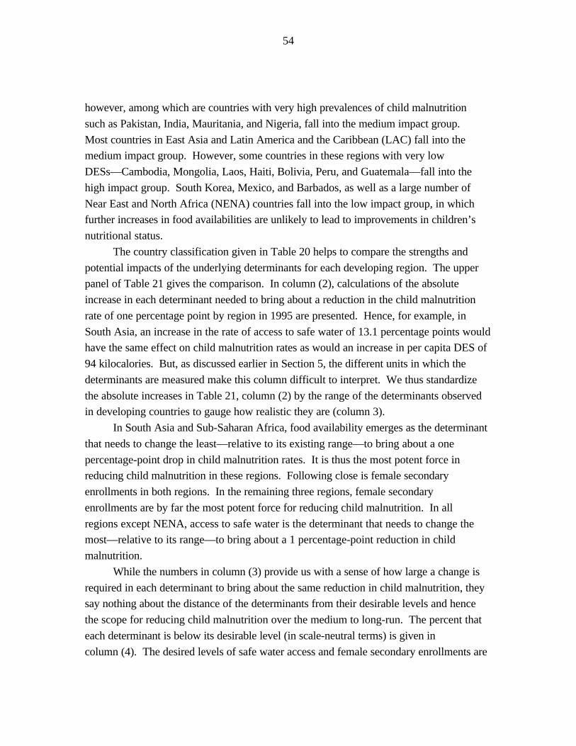
54
however, among which are countries with very high prevalences of child malnutrition
such as Pakistan, India, Mauritania, and Nigeria, fall into the medium impact group.
Most countries in East Asia and Latin America and the Caribbean (LAC) fall into the
medium impact group. However, some countries in these regions with very low
DESs—Cambodia, Mongolia, Laos, Haiti, Bolivia, Peru, and Guatemala—fall into the
high impact group. South Korea, Mexico, and Barbados, as well as a large number of
Near East and North Africa (NENA) countries fall into the low impact group, in which
further increases in food availabilities are unlikely to lead to improvements in children’s
nutritional status.
The country classification given in Table 20 helps to compare the strengths and
potential impacts of the underlying determinants for each developing region. The upper
panel of Table 21 gives the comparison. In column (2), calculations of the absolute
increase in each determinant needed to bring about a reduction in the child malnutrition
rate of one percentage point by region in 1995 are presented. Hence, for example, in
South Asia, an increase in the rate of access to safe water of 13.1 percentage points would
have the same effect on child malnutrition rates as would an increase in per capita DES of
94 kilocalories. But, as discussed earlier in Section 5, the different units in which the
determinants are measured make this column difficult to interpret. We thus standardize
the absolute increases in Table 21, column (2) by the range of the determinants observed
in developing countries to gauge how realistic they are (column 3).
In South Asia and Sub-Saharan Africa, food availability emerges as the determinant
that needs to change the least—relative to its existing range—to bring about a one
percentage-point drop in child malnutrition rates. It is thus the most potent force in
reducing child malnutrition in these regions. Following close is female secondary
enrollments in both regions. In the remaining three regions, female secondary
enrollments are by far the most potent force for reducing child malnutrition. In all
regions except NENA, access to safe water is the determinant that needs to change the
most—relative to its range—to bring about a 1 percentage-point reduction in child
malnutrition.
While the numbers in column (3) provide us with a sense of how large a change is
required in each determinant to bring about the same reduction in child malnutrition, they
say nothing about the distance of the determinants from their desirable levels and hence
the scope for reducing child malnutrition over the medium to long-run. The percent that
each determinant is below its desirable level (in scale-neutral terms) is given in
column (4). The desired levels of safe water access and female secondary enrollments are

55
The desired level of the female-to-male life expectancy ratio is determined as the average of the top34
20 percent of the data points in our panel data set, excluding the maximum value (1.15) of El Salvador in 1988,which is an extreme value compared to the other high ratios. There is no widely-accepted “desirable” levelof per capita dietary energy supplies from the stand point of nutritional health. Countries with very high levelsalso have high levels of obesity, an undesirable trait. This is the case for many high-income countries, forexample, those of Western Europe, which have an average (1995) DES of 3,360 (FAO 1998). We have alsoestimated that somewhere near a DES of 3,120 kilocalories, increases in dietary energy supplies no longerserve to reduce child malnutrition levels. Alexandratos (1995) cites the general case that 10 percent of acountry’s population will be undernourished (or food insecure) at DES levels of 2,700 kilocalories. On theother hand, FAO (1996) claims that at a level of about 2,770, only 2.5 percent of the population will beundernourished. We chose an intermediate level between 2,770 and 3,360 (of Western Europe) that is closeto 3,120 as the desired target: 3,100 kilocalories.
assumed to be 100 percent. The desired level of the female-to-male life expectancy ratio
is set at 1.01; that of per capita dietary energy supplies is set at
3,100. Column (5) gives the estimated reduction in the child malnutrition prevalence if34
each determinant were raised to its desirable level.
In all regions, increasing female secondary education to the desirable level has the
largest medium-term to long-term potential to reduce child malnutrition. Food
availability is second in Sub-Saharan Africa. Women’s relative status is second in South
Asia, East Asia, and NENA, and access to safe water is second in the LAC region.
To identify policy priorities for future reductions in child malnutrition for each
region, we rank the determinants in terms of (1) the size of the change required in them to
bring about a one percentage-point reduction in child malnutrition as a percentage of the
determinants’ ranges (based on Table 21, column 3); and (2) their scope for reducing it in
the medium-to-to long term (based on column 5). Combining these two sets of ranks, our
best estimates (in the absence of cost data—discussed below) of future policy priorities
for addressing the underlying determinants of child malnutrition in each developing
region are summarized in Table 22.
In South Asia and Sub-Saharan Africa, the top priorities are food availability and
female education. In both regions, food availability improvements have the strongest
effect, but women’s education has a strong effect and would make the biggest difference
if increased to its desirable level. In East Asia, NENA, and LAC, women’s education is
the top priority, both from the standpoint of strength of impact and scope for reducing
child malnutrition. In East Asia, food availability and women’s relative status should
also be prioritized. In NENA, women’s relative status is in second priority. In LAC,
women’s relative status and health environment improvements tie for second priority.
Health environment improvements, in a relative sense, appear to be a weak force
for reducing child malnutrition. Its low ranking is partially because there has already
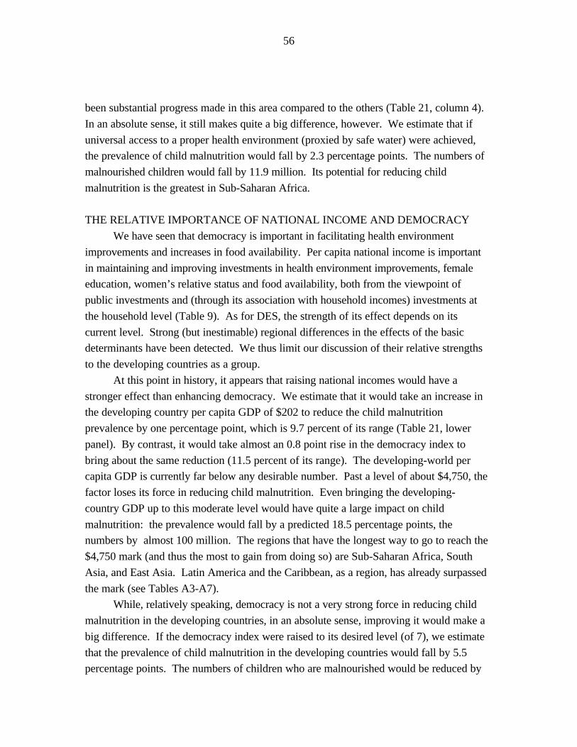
56
been substantial progress made in this area compared to the others (Table 21, column 4).
In an absolute sense, it still makes quite a big difference, however. We estimate that if
universal access to a proper health environment (proxied by safe water) were achieved,
the prevalence of child malnutrition would fall by 2.3 percentage points. The numbers of
malnourished children would fall by 11.9 million. Its potential for reducing child
malnutrition is the greatest in Sub-Saharan Africa.
THE RELATIVE IMPORTANCE OF NATIONAL INCOME AND DEMOCRACY
We have seen that democracy is important in facilitating health environment
improvements and increases in food availability. Per capita national income is important
in maintaining and improving investments in health environment improvements, female
education, women’s relative status and food availability, both from the viewpoint of
public investments and (through its association with household incomes) investments at
the household level (Table 9). As for DES, the strength of its effect depends on its
current level. Strong (but inestimable) regional differences in the effects of the basic
determinants have been detected. We thus limit our discussion of their relative strengths
to the developing countries as a group.
At this point in history, it appears that raising national incomes would have a
stronger effect than enhancing democracy. We estimate that it would take an increase in
the developing country per capita GDP of $202 to reduce the child malnutrition
prevalence by one percentage point, which is 9.7 percent of its range (Table 21, lower
panel). By contrast, it would take almost an 0.8 point rise in the democracy index to
bring about the same reduction (11.5 percent of its range). The developing-world per
capita GDP is currently far below any desirable number. Past a level of about $4,750, the
factor loses its force in reducing child malnutrition. Even bringing the developing-
country GDP up to this moderate level would have quite a large impact on child
malnutrition: the prevalence would fall by a predicted 18.5 percentage points, the
numbers by almost 100 million. The regions that have the longest way to go to reach the
$4,750 mark (and thus the most to gain from doing so) are Sub-Saharan Africa, South
Asia, and East Asia. Latin America and the Caribbean, as a region, has already surpassed
the mark (see Tables A3-A7).
While, relatively speaking, democracy is not a very strong force in reducing child
malnutrition in the developing countries, in an absolute sense, improving it would make a
big difference. If the democracy index were raised to its desired level (of 7), we estimate
that the prevalence of child malnutrition in the developing countries would fall by 5.5
percentage points. The numbers of children who are malnourished would be reduced by

57
29.4 million. The regions that have the longest way to go to reach a desirable level of
democracy are East Asia, NENA, and Sub-Saharan Africa.
The reader should bear in mind that improvements in national income and
democracy only lead to reductions in child malnutrition if they are directed to
improvements in the underlying determinants. Given enhanced political will and
education, it is possible that they can be even more effectively directed towards them in
the future than they have in the past. Our analysis gives governments an idea of where to
best direct increased national incomes in the interests of children’s nutrition. It also
suggests target areas in which political will and commitment among democratic
governments can be instilled.
A NOTE ON COST-EFFECTIVENESS
On a final note, for a full assessment of priorities for the future, we would ideally
want to take into account the costs of improving the alternative determinants. While the
same reduction in child malnutrition could be brought about by a 13.1 percentage-point
increase in access to safe water as a 4.6 percentage-point increase in female secondary
enrollments, it is unlikely that these increases would cost the same. Their costs are likely
to differ by region as well. Unfortunately, good quality comparative information on cost-
effectiveness of these different policies is lacking. One can still get a sense of how
different the relative costs have to be before the conclusions reached on priorities are
altered. For example, if it cost more than 2.8 times as much to increase female secondary
enrollment by one percent compared to the costs of increasing access to safe water by one
percent, then the latter will be the more cost-effective investment in reducing
malnutrition. If the ratio is below 2.8, then female secondary education becomes more
cost-effective. Better information on cost-effectiveness should be the focus of future
research on policies to improve child nutritional status.
9. SUMMARY AND CONCLUSIONS
Thirty percent—167 million—of all developing-country children under five are
currently malnourished. The overall objective of this study was to use historical cross-
country data to improve our understanding of the relative importance of the various
causes of this malnutrition for the developing countries as a whole and by region. In this
way, we hoped to contribute to the debate on how to make the best use of available

58
Box 2: The (South) Asian Enigma
South Asia’s child malnutrition prevalence is 50 percent. Sub-Saharan Africa’s is 31 percent.Why is South Asia’s so much higher? The great difference has recently been called an“enigma” because South Asia as a region is doing so much better than Sub-Saharan Africafor most of the determinants of child malnutrition (see Box Table 2) (Ramalingaswami,Johnsson, and Rohde 1996). There are three possible sources of the differences.
The first is that the determinants of child malnutrition are different or have different strengthsof impact in the regions. If one were more important in South Asia, and South Asia is notdoing very well in the area—regardless of how well Sub-Saharan Africa is doing, then thatdeterminant would be a clue to the enigma. This study finds no major differences betweenthe regions in terms of the importance of the underlying determinants of childmalnutrition—health environment, women’s education and relative status, and national foodavailability—as causal factors. For the basic determinants, however, we find that democracyand national income are more important in South Asia than the other regions, including Sub-Saharan Africa. South Asia is doing fairly well in the area of democracy. Even though it isdoing better than Sub-Saharan Africa in the area of national income, it is still doing verypoorly. Since this factor is more important in determining child malnutrition in South Asia thanin Sub-Saharan Africa, it may be one reason why South Asia is doing worse. Since nationalincome is so strongly linked with poverty, and South Asia is also doing poorly (even worsethan Sub-Saharan Africa) in this area, it may also be a clue.
The second possible source of the difference in the regions’ child malnutrition rates is that,of the determinants we have considered that are equally important in the regions, South Asiais doing worse than Sub-Saharan Africa. Box Table 2 shows that South Asia is doing betterthan Sub-Saharan Africa in all these areas except women’s relative status. We can thussurmise that, among the observed determinants in child malnutrition that we have consideredin this study—those that change over time, women’s status is a primary reason for theregion’s differing prevalences.
The final source of the difference in the regions’ child malnutrition rates lies in the “blackbox” of unobserved, time-invariant country-specific factors. Because our data setcovers more than one point in time for each country, we have been able to estimate theeffects on child malnutrition of these factors. They are found to raise South Asia’s childmalnutrition prevalence above Sub-Saharan Africa’s substantially. To illustrate theirimportance in the regional differences, Box Figure 1 shows how much child malnutritionwould remain even if all of the underlying determinants were raised to their desirable levels.In South Asia, a 23.8 percent prevalence would remain, but only 0.5 percent in Sub-SaharanAfrica. These deeply-entrenched factors somehow specific to South Asian countries, then,are also key to solving the Asian Enigma. In the long run, if child malnutrition is to beovercome in the region, attention must be paid to opening the black box to find out what theyare and implementing policies to address them. Some possibilities are a monsoon climate(FAO 1996), including recurrent flooding in some countries, overcrowding due to highpopulation density, and cultural beliefs and traditions that hinder optimal breast-feeding andtiming of the introduction of complementary foods (Ramalingaswami et al. 1996).

59
resources to reduce malnutrition in developing countries now and in the coming years to
2020.
The conclusions of the study are based on estimations undertaken with careful
consideration to data quality and statistical soundness. The study is guided by a well-
accepted, comprehensive conceptual framework. It employs household survey-based
nationally-representative underweight prevalence data that have been subjected to strict
quality control standards. It employs an estimation methodology that yields unbiased
parameter estimates. Specification test results indicate that the models estimated are a
reasonably good representation of the quantitative relationships between child
malnutrition and its determinants and that we have done the best we can, given available
data, to identify a causal relationship between them. We thus believe that we have
succeeded in our goal of making maximum use of the available data.
The estimation results in Section 5 show that all four of our variables representing
the underlying determinants of child malnutrition—health environments, women’s
education, women’s relative status, national food availability—have significant impacts
on child malnutrition. The basic determinants—national income and democracy—have
strong impacts through facilitating investment in the underlying determinants.
The study has found weak evidence of a feed-back effect of child malnutrition, i.e.,
that child malnutrition today, regardless of future levels of its determinants, contributes to
greater levels of child malnutrition in the future. The existence of this linkage suggests
that reducing child malnutrition at a fast pace today should reduce child malnutrition in
the future at an even faster pace.
Section 6 presented estimations of the contribution each determinant made to the
15.5 percentage-point reduction in the prevalence of child malnutrition from 1970 to
1995. Among the underlying determinants, increases in women’s education have made
the greatest contribution, being responsible for 44 percent of the total reduction.
Improvements in food availability contributed to 26 percent of the reduction, health
environment improvements to 19 percent. Because there has been little improvement in
women’s relative status, its contribution—while still substantial—was the lowest (12
percent). In South Asia, in addition to women’s education, particularly large
contributions were made by improvements in women’s relative status and health
environments. While South Asian countries’ per capita food availabilities deteriorated
during the world food crisis of the early 1970s, improvements in the 1980s made a large
contribution. In Sub-Saharan Africa, reductions in child malnutrition have taken place
largely through increases in women’s education and health environment improvements.
Per capita food availability made very little contribution overall, although its positive

60
impact on child nutrition in the last 10 years has demonstrated its future potential.
Declines in women’s relative status in the region have muted the positive impacts of the
other determinants. In East Asia and the Near East and North Africa (NENA), increases
in women’s education and food availability have made the greatest contributions. In the
Latin America and Caribbean (LAC) region, women’s education has been a major
contributor throughout the 25 years. The other determinants have made little
contribution, especially in recent years.
In terms of the basic determinants, improvements in per capita national income
have made a substantial contribution, an estimated 7.4 percentage-point reduction in the
developing-country prevalence of child malnutrition. The contribution was positive for
all regions except Sub-Saharan Africa. While democracy has a potentially large
contribution to make, because little progress has been made in this area, its overall
contribution has been minimal. Deteriorations in democracy have had a negative impact
on child malnutrition in South Asia and East Asia.
The analysis in Section 7 projects the prevalence and numbers of malnourished
children in the year 2020 under three scenarios for growth in the four underlying
determinants. The status quo scenario assumes that the nonfood determinants increase at
the rate they did over the 1985-95 period. For food availability, we use IFPRI IMPACT
model projections (Rosegrant, Agcaoili-Sombilla, and Perez 1995). The pessimistic
scenario assumes a 25 percent cut in the rate of change of the nonfood determinants plus
the low investment IMPACT model projection for food availability. The optimistic
scenario assumes a 25 percent increase in the rate of change of the nonfood determinants
plus the high investment IMPACT model projection for food availability. Under the
status quo scenario, 18 percent of developing-country children under five are projected to
be malnourished in 2020. The prevalence rises to 22 percent under the pessimistic
scenario and falls to 15 percent under the optimistic scenario. The payoffs to the
optimistic scenario can be best realized in Sub-Saharan Africa and South Asia. What is
particularly striking is that even under an optimistic scenario, the absolute numbers of
malnourished children in Sub-Saharan Africa will be higher in 2020 than they are in
1995. Based on the status quo projections, we predict a sharp regional shift in the
location of child malnutrition: South Asia’s share will fall from 51 percent in 1995 to 47
percent in 2020, but Sub-Saharan Africa’s share will increase from 19 percent in 1995 to
near 35 percent in 2020.
Section 8 assesses the relative effectiveness of the four underlying determinants in
terms of their potential for generating future reductions in child malnutrition. This
exercise is undertaken in the absence of crucial cost-side information. The data indicate

61
Note that simply maintaining the determinants at their 1995 levels will require substantial resources,35
particularly for national per capita food availability, which has to be maintained in the face of increasingpopulations and a fairly fixed amount of cultivable land.
that improvements in per capita food availability and in women’s education offer the best
hope for future reductions in child malnutrition in Sub-Saharan Africa and South Asia. In
East Asia, NENA, and LAC, the first priority is women’s education. For East Asia, the
second priorities are food availability and women’s relative status. In NENA, the second
priority is women’s relative status. In LAC, they are women’s relative status and health
environment improvements. Actions associated with these priorities should be seen as35
complementary to more direct measures that have been the traditional focus of nutrition
interventions, such as breast-feeding promotion and food fortification.
The study contributes to the resolution of five important debates currently
underway in development policy and research circles. First, why has child malnutrition
been rising in Sub-Saharan Africa? Here, all we can say is that some of the increase is
due to the declining relative status of women and deteriorations in per capita national
incomes (and thus rising poverty). Debt and structural adjustment, increasing conflict
levels, and the rise of HIV/AIDS may also be responsible, and this should be the subject
of future research.
Second, why are child malnutrition rates in South Asia so much higher than in Sub-
Saharan Africa? This study identifies two key variables at the source of the “Asian
enigma”: women’s relative status (which is much worse in South Asia) and national
income (very low in South Asia yet a particularly important determinant of child
malnutrition there). Poverty (higher in South Asia), may also partially explain the
regions’ differences. Regardless of the levels of the determinants of child malnutrition
that we have identified in this study, a large disparity in child malnutrition prevalences
between the regions would persist. The source of this remaining difference is time-
invariant factors specific to South Asian countries that we have been unable to identify
explicitly. Examples might be the region’s monsoon climate, high population densities,
and deeply-entrenched beliefs regarding child feeding practices. An unraveling of this
“black box” should also be the subject of further research.
Third, how important of a determinant of child malnutrition is food availability at a
national level? We find national food availability to be a particularly important
determinant of child malnutrition when it is at very low levels (below approximately
2,300 kilocalories). After a certain point (approximately 3,120 kilocalories), further
improvements are unlikely to aid in reducing child malnutrition. For countries with such

62
high food availabilities, efforts to promote food security must be focused on promoting
food access at the household level. The regions in which improved food availabilities
have the most to contribute in the coming decades are South Asia and Sub-Saharan
Africa.
Fourth, how important are women’s status and education? This research report
confirms the now overwhelming evidence of the strong impact of women’s education on
children’s nutrition. The report also establishes that women’s relative status is an
important determinant of child malnutrition in all developing country regions. These
findings confirm women’s key role in the etiology of child nutrition, whether through the
pathway of maternal and child care or household food security. Together, improvements
in women’s education and status alone contributed to over 50 percent of the reduction in
child malnutrition that took place from 1970 to 1995. More emphasis should be placed
on them in the future than has been in the past—especially on women’s status and
education in South Asia and women’s education in Sub-Saharan Africa.
Fifth, how important are national political factors (such as democracy) and national
incomes, and through what pathways do they affect child malnutrition? This report has
established the existence of a significant link between the degree of democracy in
countries and their prevalence of child malnutrition, with democracy working mainly
through improving health environments and national food availability. Why it is
important for these two underlying determinants and not for others needs to be better
understood. Nevertheless, the analysis suggests that political variables have as valid a
place in studies of malnutrition as they do in studies of economic growth. National
income is an even more important determinant of child malnutrition than democracy.
Increases in per capita national income have contributed to almost half of the total
reduction in the developing-country child malnutrition prevalence of 1970-95, working
via all four underlying determinants.
A key message of this paper is that any comprehensive strategy for attacking the
problem of child malnutrition must include actions to address both its basic and
underlying causes. If national incomes and democracy are not improved, the resources
and political will necessary for investing in health environments, women’s education and
status, and food availabilities will not be available. If improved national incomes and
democracy are not directed at improvements in the underlying determinants, on the other
hand, they will make little difference.
Before concluding, we point to some limitations of the study. The first is our
inability to adequately consider two factors believed to have a strong influence on child
malnutrition: food security at the household level and poverty. With respect to the

63
former, at the present time there are no cross-country comparable data on national rates of
food insecurity from household survey data (Smith 1998b). In its place, we have
employed per capita dietary energy supplies, an inadequate measure of food insecurity
because they do not measure food access. With respect to poverty, while some data exist
(World Bank 1998b), at present there are not enough to reliably estimate this variable’s
influence on child malnutrition. The second main limitation of this study is our inability
to address the sequential nature of optimal interventions for improving child nutritional
status. In many cases, one intervention, for example, provisioning of health services, will
need to be undertaken before others will have any positive impact. Our estimation
methodology limits us to estimating each explanatory variable's impact as if interventions
were to take place simultaneously. A third limitation of the study is that we are unable to
consider the cost-effectiveness of various interventions in the setting of policy priorities.
We can suggest several fruitful directions for future research. The first is to
undertake the analysis for rates of stunting, which is a longer term measure of nutritional
deprivation than is underweight. The second is to undertake estimations separately for
male and female under-fives to determine if malnutrition among these groups is explained
by different factors. Corresponding to the limitations identified, we see a need for future
research into the sequencing of interventions to improve child nutrition and into the costs
of various interventions to improve child nutrition. Fourth, a more in-depth
understanding of the little-studied roles of democracy and women's status are needed.
Fifth, the roles of debt and structural adjustment, conflict, and HIV/AIDS in Sub-Saharan
Africa’s rising malnutrition and of the time-invariant factors explaining South Asia’s
higher child malnutrition prevalence need to be investigated.
Finally, an indicator of national prevalences of food insecurity—based fully on
household food consumption survey data—is needed for clarifying the role of this
important determinant of child malnutrition and for identifying where food insecurity is
located and how it changes over time. While in the past the task was held back by data
availabilities, with the increased frequency of household food consumption surveys, the
development of such an indicator is now possible.
In conclusion, we hope that this study will aid policymakers that have a broad
international mandate to prioritize their resource investments in the goal of reducing and
eventually eliminating malnutrition in the developing countries. We hope that it will
instigate further investigation into the importance of the factors affecting child
malnutrition that we have highlighted, particularly those that have received relatively
little attention in the past: women’s status and democracy.

64
We end with a caution to users of this study’s findings: the results apply only at the
very broad level of the developing countries as a whole and, more tentatively, to the
developing-country regions. Their applicability to specific populations at more
disaggregated levels is unknown. Careful analysis and diagnosis are needed for
understanding the causes of child malnutrition for each subpopulation of the developing
world, whether it be a country, a subnational region, a community, a household, or an
individual child.

65
TABLES

66
Table 1. Trends in Developing-Country Child Malnutrition (Underweight) by Region, 1970-1995Percent Underweight Numbers underweight
Region 1970 1975 1980 1985 1990 1995 Change 1970 1975 1980 1985 1990 1995 Change1970-95 1970-95
(percent) (millions of under-fives)
South Asia 72.3 67.7 63.7 55.3 53.4 49.3 -23.0 96.7 90.6 89.9 87.2 95.4 86.0 -10.7
Sub-Saharan Africa 35.0 31.4 28.9 25.8 28.8 31.1 -3.9 20.6 18.5 19.9 20.9 25.7 31.4 +10.8
East Asia 39.5 33.3 30.0 28.8 23.5 22.9 -16.6 53.5 45.1 43.3 45.3 42.5 38.2 -15.3
Near East and North Africa 20.7 19.8 17.2 13 14.6 -6.1 5.4 5.2 5.0 4.1 6.3 +0.9not notavailable available
Latin America and the 21.0 17.0 12.2 12.9 11.4 9.5 -11.5 10.1 8.2 6.2 6.3 6.2 5.2 -4.9Caribbean
Total 46.5 41.6 37.8 34.3 32.3 31.0 -15.5 187.3 167.6 164.3 163.8 176.7 167.1 -20.2
Sources: 1975, 1980 and 1985 prevalences and numbers of malnourished children are from Table 1.2 of ACC/SCN (1992); 1990 and 1995 estimates are from WHO(1997), Table 6. The prevalences for 1970 are predicted using the underlying-determinant model regression results presented in Section 5.2.1 of this paper.
Notes: A child under five (0-59 months) is considered malnourished if the child falls below an anthropometric cutoff of -2 standard deviations below the median valueof weight-for-age using National Center for Health Statistics/World Health Organization standards. ### 1970 numbers of underweight approximated using 1975total numbers of children while awaiting estimates from UN Population Prospects 1996 Revision.

67
Table 2. Regional, Country and Population Coverage of the Study
Region Number Regional Number Countries of Coverage (in of
Count- terms of Obser-ries number of vations
countries)
South Asia 5 71% 16 Bangladesh(82, 85, 89, 96), India-rural(77, 91), Nepal-rural(75, 95), Pakistan(77, 85, 90, 95), Sri Lanka(77,80, 87, 93).
Sub-Saharan 26 58% 65 Benin(87, 96), Burkina Faso(87, 92), Cameroon(77,Africa 91), Comoros(91, 95), Congo, Rep.(77, 87), Congo,
Dem. Rep.(75, 86, 89, 94), Côte d'Ivoire(86, 94),Ethiopia-rural(83, 92), Ghana(87, 93), Guinea(80, 95),Kenya-rural(82, 87), Lesotho(76, 81, 94),Madagascar(83, 92, 95), Malawi(81, 92, 95),Mauritania(81, 87, 90), Mauritius(85, 95), Niger(85,92), Nigeria(90, 93), Rwanda(76, 92), Senegal(86, 92),Sierra Leone(74, 77, 90), Tanzania(87, 91, 96),Togo(76, 88), Uganda(77, 88, 95), Zambia(72, 85, 88,92, 96), Zimbabwe(84, 88, 94).
East Asia 8 57% 26 China(87, 92, 95), Indonesia(78, 87, 95), Laos(84, 94),Malaysia(83, 86, 90, 95), Myanmar(80, 83, 90, 95),Philippines(73, 82, 87, 93), Thailand(82, 87, 90),Vietnam(80, 87, 94).
Near East and 5 31% 14 Algeria(87, 92, 95), Egypt(78, 88, 92, 95), Jordan(75,North Africa 90), Morocco(87, 92), Tunisia(74, 88, 94). (NENA)
Latin 19 68% 58 Bolivia(81, 89, 93), Brazil(75, 89, 96), Chile(78, 82, 86,America and 95), Columbia(77, 86, 89, 95), Costa Rica(78, 82, 89,the Caribbean 94), Dominican Republic(86, 91), El Salvador(88, 93),(LAC) Guatemala(77, 80, 87, 95), Guyana(71, 81, 93),
Haiti(78, 90, 94), Honduras(82, 87, 93), Jamaica(78, 85,89, 93), Mexico-rural(74, 79, 89), Nicaragua(80, 93),Panama(80, 92), Peru(75, 84, 91, 96), Trinidad andTobago(76, 87), Uruguay(87, 92), Venezuela(81, 87,90, 94).
TOTAL 63 57% 179
(88 % of totaldeveloping
worldpopulation)a
This percentage is calculated from countries’ 1995 populations. a
Note: See Appendix Table A8 for regional grouping of developing countries.

68
Table 3. Variable Definitions and Sample Summary Statistics
Variable Definition Mean Standard deviation Minimum Maximum
Child Malnutrition Percent of children with weight-for-age less than 2 standard 24.6 15 0.9 71.3(CHMAL) deviations from the mean according to NCHS/WHO standards (%) (Chile 1995) (India 1977)
Access to Safe Water Percent of population with access to safe water (%) 56.2 23.7 6 100(SAFEW) (Ethiopia 1983) ( Mauritius 1985)
Female Secondary Gross female secondary school enrollment rate (%) 33.8 22.5 2.5 88Enrollments (Uganda 1977) (Uruguay 1992)(FEMSED)
Female to Male Life Ratio of female life expectancy at birth to male life expectancy at 1.062 0.03 0.97 1.15Expectancy Ratio birth (Nepal 1975) (El Salvador 1988)(LFEXPRAT)
Per capita Dietary Daily per capita dietary energy supply (kilo calories) 2360 331 1592 3284Energy Supply (DES) (Ethiopia 1992) (Egypt 1995)
Per capita National Per capita Gross Domestic Product (in purchasing power parity - 2306 1779 306 8612Income (GDP) adjusted 1987 U.S. dollars) (Ethiopia 1992) (Chile 1995)
Democracy Combined index of political rights and civil liberties (measured on a 3.5 1.7 1 7(DEMOC) scale of 1 to 7 points, 1=least democratic) (Costa Rica 1978,
a
1982, 1989)The countries for which the democracy index number is 1 are: Algeria (1995), Benin (1987), China (1992, 1995), Ethiopia (1983), Guinea (1980), Haiti (1994), Laos (1994), Mauritaniaa
(1995), Myanmar (1990, 1995), Uganda (1977),Vietnam (1980, 1987, and 1994), and Zaire (1986).

69
Table 4. Regional Comparison of Sample Underweight Prevalences and Explanatory Variable Means, 1970s-1990s
Child Access to Female Secondary Female to Male Life Per capita Dietary Per capita Democracy Malnutrition (%) Safe Water (%) Enrollments Expectancy Ratio Energy Supply National Income (1=least democratic)
(1) (2) (3) (4) (5) (6)(%) (kilo calories) ($PPP) (7)
South Asia 61 60.5 23.8 1.010 2187 863 4.59
1970s (n=4) 69.1 29.8 16.3 0.987 2023 728 4.38
1980s (n=6) 61.8 51.9 14.2 1.020 2042 719 3.25
1990s (n=6) 55.7 81.3 31.5 1.022 2332 990 5.16
Sub-Saharan Africa 31 37.5 15.6 1.061 2164 879 2.57
1970s (n=10) 27.2 24.7 8.5 1.069 2207 1358 1.77
1980s (n=26) 26.5 35.0 14.6 1.066 2117 1031 2.02
1990s (n=29) 33.7 40.4 17.0 1.060 2184 740 2.96
East Asia 23 64.5 47.9 1.051 2595 1874 1.69
1970s (n=2) 45.0 19.7 25.8 1.050 2007 1402 3.0
1980s (n=13) 26.8 63.8 39.2 1.053 2502 1483 2.30
1990s (n=11) 19.4 67.8 54.4 1.049 2686 2132 1.25
Near East/North Africa 11 75.5 52.5 1.043 3058 2527 2.81
1970s (n=3) 16.5 72.5 34.0 1.042 2710 1547 3.32
1980s (n=4) 10.1 69.3 46.4 1.043 3018 2746 3.09
1990s (n=7) 10.8 79.4 59.7 1.043 3157 2637 2.55
Latin America/Caribbean 12 71.8 44.8 1.094 2647 4740 4.73
1970s (n=12) 18.9 59.5 33.3 1.086 2620 4713 4.06
1980s (n=26) 11.4 79.0 47.2 1.096 2675 4871 5.14
1990s (n=20) 8.3 73.3 51.4 1.098 2636 4607 4.79
Note: The means reported in this table are calculated based only on the country-year pairs included in the study data set. They are population-weighted.

70
Table 5. Underweight Prevalences and Explanatory Variable Means, 1970s-1990s
1970s 1980s 1990s Change % change1970s-1990s 1970s-1990s
Child Malnutrition (%) 50.7 29.0 28.5 22.2 -43.8
Access to Safe Water (%) 36.3 61.6 69.0 32.7 +90
Female Secondary Enrollments (%) 21.7 34.5 45.0 23.3 +107
Female to Male Life Expectancy Ratio 1.024 1.055 1.047 0.023 +2.25
Per capita Dietary Energy Supply 2,187 2,440 2,564 377 +17.2
Per capita National Income 1,772 1,871 1,904 132 +7.45
Democracy (1=least democratic) 3.96 2.86 2.66 -1.3 -32.8
Number of observations 31 75 73 -- --
Number of countries 29 54 58 -- --Note: The means reported in this table are calculated based only on the country-year pairs included in the
study data set and therefore must be considered illustrative (see Table 11 for an alternativeestimation of the changes in time using data on all of the study countries for consecutive five-yearintervals). They are population-weighted.
Table 6. Regional Poverty Prevalences for 1987, 1990, and 1993
1987 1990 1993
South Asia 45.4 43 43.1
Sub-Saharan Africa 38.5 39.3 39.1
East Asia 29.7 28.5 26
Near East and North Africa 4.7 4.3 4.1
Latin America and the Caribbean 22 23 23.5
TOTAL 33.9 32.9 31.9
Source: Ravallion and Chen (1996) Table 5Note: The poverty measure employs an international poverty line of $1 per person per day at 1985
purchasing power parity. .

71
Table 7. Ordinary Least Squares and Country Fixed-Effects Estimation Results:Linear Specifications
Ordinary Least Squares Country Fixed-Effects
Underlying- Basic- Underlying- Basic- AllDeterminants Determinants Determinants Determinants Determinants
(1) (2) (3) (4) (5)
Access to safe water(SAFEW)
-.139 -.085 -.069 (2.7)*** (2.14)** (1.7)*
Female secondary -.068 -.167 -.177 enrollments (1.27) (2.64)*** (2.78)***(FEMSED)
Female-to-male life -177 -93.45 -111expectancy ratio (5.23)*** (2.25)** (2.6)**(LFEXPRAT)
Per capita dietary -.012 -.0081 -.0077energy supply (DES) (3.65)*** (2.48)** (2.21)**
Per capita national -.0048 -.0023 1.20 E-04income (GDP) (8.2)*** (2.46)** (.137)
Democracy -.274 -.884 -.779(DEMOC) (.44) (1.67)* (1.68)*
R-Squared .433 .346 .943 .916 .945
Adjusted R-Squared .420 .338 .910 .869 .910
Notes: The dependent variable is prevalence of child malnutrition. The number of observations for allregressions is 179 (63 countries). Absolute values of t-statistics are given in parentheses. *indicates significance at the 10% level; ** indicates significance at the 5 percent level; ***indicates significance at the 1 percent level.

72
Table 8. Country Fixed-Effects Estimation Results: Non-Linear SpecificationsQuadratic Three-Segment Linear Spline
DES and GDP Curves DES and GDP Curves
Underlying Basic Underlying BasicDeterminants Determinants Determinants Determinants
(1) (2) (3) (4)
Access to safe water (SAFEW) -.072 -.076 (1.84)* (1.95)*
Female secondary enrollments -.232 -.220(FEMSED) (3.51)*** (3.41)***
Female-to-male life expectancy ratio -74.89 -71.8(LFEXPRAT) (1.83)* (1.74)*
Per capita dietary energy supply -.067 (DES) (3.00)***
DES-squared 1.24 E-05 (2.66)***
DES Spline -.0170 DES # 2300 (n=93) (3.41)***
2300< DES#3120 (n=83) -.0024 (2.16)**
DES > 3120 (n=3) .0405(1.35)
Per capita national income (GDP) -.0121 (4.68)***
GDP-squared 9.67 E-07 (4.03)***
GDP Spline -.0444 GDP # 800 (n=37) (3.15)***
800< GDP# 4725 (n=118) -.0067 (2.63)***
GDP > 4725 (n=24) .0006 (3.37)***
Democracy (DEMOC) -1.45 -1.27(2.81)*** (2.51)**
R-Squared .947 .927 .947 .930
Adjusted R-Squared .914 .884 .914 .889
Notes: The dependent variable is prevalence of child malnutrition. The coefficients on the fixed-effects terms are notshown. The number of observations for all regressions is 179 (63 countries). Absolute values of t-statisticsare given in parentheses. * indicates significance at the 10 percent level; ** indicates significance at the 5percent level; ***indicates significance at the 1 percent level.

73
Table 9. Country Fixed-Effects Estimates of the Effects of Per capita NationalIncomes and Democracy on Underlying-Determinant ExplanatoryVariables
Access to Safe Female Female to Male Per capitaWater Secondary Life Expectancy Dietary Energy
(SAFEW) Enrollments Ratio Supply
(1) (2) (3) (4)(FEMSED) (LFEXPRAT) (DES)
Per capita national .0174 .0148 1.0 E-05 .4105income (GDP) (2.85)*** (3.71)*** (1.90)* (6.26)***
GDP-squared -1.31 E-06 -9.32 E-07 -8.2 E-10 -2.79 E-05 (2.31)** (2.53)** (1.67)* (4.59)***
Democracy (DEMOC) 3.49 .981 -.002 26.28 (2.87)*** (1.23) (1.57) (2.0)**
R-Squared .835 .922 .901 .902
Adjusted R-Squared .740 .877 .845 .846
Notes: The number of observations for all regressions is 179 (63 countries). Absolute values of t-statisticsare given in parentheses. * indicates significance at the 10 percent level; ** indicates significanceat the 5 percent level; ***indicates significance at the 1 percent level.

74
Table 10. Instrumental Variable Candidates for Hausman-Wu Endogeneity Tests
Explanatory Candidate Instrument Rationale for Instrument Choice Data Source CorrelationVariable between
instrument andvariablea
Population with (1) Annual internal Freshwater availability is unlikely to affect child malnutrition other than through World Resources 0.19access to safe renewable freshwater provision of safe water. Institute (p=.043)water (SAFEW) resources per capita (various years)
Female secondary (2) Male gross primary Current male primary enrollments unlikely to be contemporaneously correlated with UNESCO(1998) 0.55enrollments enrollments malnutrition of under-fives, yet to be correlated with female secondary enrollments (p=.000)(FEMSED) through the value placed on education and through its availability.
Female-Male Life (3) Percent of births Births attended by health staff likely to be (positively) correlated with female life UNICEF State of the 0.39Expectancy Ratio attended by health staff expectancy through reduced maternal mortality yet not to affect the nutritional status of World’s Children (p=.000)(LFEXPRAT) surviving children. (various years) and
World Bank (1997a)
Per capita dietary (4) Arable land per capita Land availability is a constraining factor in agricultural production; However, could FAO (1998) -0.10energy supply affect child malnutrition through raising incomes from non-food production. (p=.17)(DES)
(5) Land under cereal Land employed as an input into cereal production raises food production. My affect FAO (1998) -0.19production per capita child malnutrition other than through DES by raising incomes. (p=.014)
(6) Fertilizer use per Fertilizer use increases agricultural yields; May affect child malnutrition other than FAO (1998) 0.49hectare of arable land through DES by raising incomes or causing illness in children due to leakage of (p=.000)
contaminants into water tables.
(7) Irrigated land per The use of irrigation increases agricultural yields; However, could affect child FAO (1998) 0.20capita malnutrition other than through DES by raising household incomes. (p=.009)
Per capita Gross (8) Real investment share As per Pritchett and Summers (1996). World Bank (1997a, 0.31Domestic Product of GDP 1998) (p=.000)(GDP)
(9) Foreign investment As per Pritchett and Summers (1996). World Bank (1997a, 0.25share of GDP 1998) (p=.001)
(10) Economic openness Economic openness may improve national income but not otherwise affect child Penn World Tables 0.07measure malnutrition. (p=.367)
Democracy No candidate identified. -- -- --(DEMOC)
Pearson correlation coefficient between nonmissing values for entire sample. If the p-value (given in parentheses) is greater than 0.1, the correlation is considered to be statisticallya
insignificant.

75
Table 11. Results of Endogeneity Tests
Explanatory Variable Instrumental Number Relevance Overidentification Hausman-Wu Variable(s) of (3) (4) (5)
observ-ations
a b c
F Test P Test t Teststatistic passed? statistic passed? statistic passed?
2
Population with access to Water resources 94 3.4* yes -- -- 1.2 yessafe water (SAFEW)
Female secondary Male primary 179 0.67 no -- -- --enrollments (FEMSED) enrollments
notperformed
Female-to-male life Birth attendance by 92 0.46 no -- -- --expectancy ratio health staff(LFEXPRAT)
notperformed
Per capita dietary energy Land in cereal, fert- 163 2 no -- -- --supply (DES) ilizer use, irrigated land
notperformed
Fertilizer use, irrigated 177 3.1** yes 0.7 yes 1.4 yesland
Per capita national income Investment share and 164 8.9*** yes 0.35 yes -0.27 yes(GDP) foreign investment
share of GDP
Notes: These tests are only performed for the fixed-effects model specifications, with quadratic terms representing nonlinearities.The null hypothesis is that the instrument set z in a regression of the potentially endogenous variable on the exogenous variables and z is not (jointly)a
significant. If F is greater than the critical value of the F-distribution for 1% (***), 5% (**), or 10% (*) level tests, then the null hypothesis isrejected.The null hypothesis is that the model is correctly specified (the instruments should not be included in the list of explanatory variables) and theb
instruments z are uncorrelated with the error term in the CHMAL equation. The chi-squared statistic is equal to n*R , where n is the number of2
observations and R is from a regression of the predicted residuals from Two Stage Least Squares estimation of the original CHMAL regression on2
the exogenous variables plus z. This test can only be performed when there is more than one instrument available for the variable being tested. It isnot possible to perform the test using the non-linear (quadratic) specifications because DES and GDP are too highly correlated with their squares. The test results reported are for the associated linear models. We assume that if the instruments for the variables pass the test in the linear models,then they are uncorrelated with the error term in the non-linear models.The null hypothesis being tested is that the Instrumental Variable and fixed-effects estimates are different, indicating endogeneity of the variable. c
The null hypothesis is rejected if the predicted residuals from a regression of the endogenous variable on the exogenous variables and instruments areinsignificant when included in a regression of CHMAL on all explanatory variables. The statistics are corrected using a procedure laid out inHaddad et al. 1995.

76
Table 12. How Strong Are the Effects on Child Malnutrition? Elasticities and Related Statistics for theirInterpretation
sample Elasticity developing- Increase in variable needed number in (5) as a(or evaluated at country to reduce prevalence of percent of
segment) sample mean range child malnutrition by one developing-mean percentage point country range (1) (2) (3) (4) (5)
a
b
c
Underlying-Determinant Variables Population with access to safe water (SAFEW) 56.2 -0.174 1 - 100 13.1 13.2
Female secondary enrollments (FEMSED) 33.8 -0.302 4.6 4.60.5 - 100
Female-to-male life expectancy ratio 1.0624 -3.092 0.97 - 1.12 0.0139 9.3 (LFEXPRAT)
Per capita dietary energy supply (DES) 2360 -0.949 1,522 - 3,605 101 4.9
DES#2300 2106 -1.150 59 2.8
2300<DES#3120 2613 -0.343 425 20.4
DES > 3120 3230 0 -- --
Basic-Determinant Variables Per capita national income (GDP) 2306 -1.26 300 - 8612 74.1 0.89
GDP # 800 645 -0.740 23 0.3
800< GDP# 4725 2102 -0.605 150 1.8
GDP > 4725 5867 0.329 -- --
Democracy (DEMOC) 3.5 -0.181 1 - 7 0.79 13.1
Estimated percent change in CHMAL resulting from a 1 percent increase in the explanatory variable based on estimates of Table 8, columns (3) anda
(4). The segment elasticities for DES and GDP are evaluated at the variable and CHMAL means for the data falling within the segments. The endpoints of the developing country ranges are for the following countries and years (min, max): SAFEW (Gabon 1970; Barbados 1990s),b
FEMSED (Mauritania 1970; Bahrain 1993); LFEXPRAT (Nepal 1975, max: Brazil 1996 and El Salvador 1993). Note: These numbers are onlybased on this study’s sample and the maximum value for the sample, that of 1.15 for El Salvador in 1988 is excluded); DES (Ethiopia 1977, Turkey1995); GDP (Ethiopia 1992; Chile 1995); DEMOC (see Table 3 for examples from this study’s sample). Calculated as 1 divided by the regression coefficients of Table 8, columns (3) and (4).c

77
Table 13. Estimated Regression Coefficients for Dietary Energy Supply Per capitaand Gross Domestic Product Per capita by Region (1970-95)
Dietary Energy Supply Per Gross Domestic Product PerCapita Capita
mean coefficient mean coefficient(1) (2) (3) (4)
South Asia 2,187 -0.0133 863 -0.0255
Sub-Saharan Africa 2,164 -0.0140 879 -0.0222
East Asia 2,595 -0.0085 1,874 -0.0090
Near East and North Africa 3,058 -0.0019 2,527 -0.0067
Latin America and the Caribbean 2,647 -0.0069 4,740 -0.0040
Full Sample 2,360 -0.0099 2,306 -0.0135a
Notes: The coefficients are calculated as a weighted average of the segment coefficients, where theweights are the proportion of the sample data points of the region falling into each segment.
While the regional means are population-weighted, the full sample means are not (see Table 3).a

78
Table 14. Dynamic Estimation Results—Basic Determinants
Ordinary Least Squares Country Fixed-Effects
(1) (2) (3)
Without time trendand initial With time trend andconditions initial conditions
Lagged Child Malnutrition .76 .290 .454 (19.3)*** (1.41) (.941)
Per capita National Income -.001 -.745 -.0016(GDP) (2.92)*** (1.0) (.95)
Democracy (DEMOC) -.931 -.0008 -1.27 (2.64)*** (.61) (1.32)
Time trend (t) .52(1.33)
t*GDP0 .0006(.87)
t*DEMOC0 -.903(1.57)
R-Squared .856 .0605 .1102
# Countries 63 36 36
# Observations 116 54 54
Note: The dependent variable is the prevalence of underweight children under five. Absolute values of t-statistics are given in parentheses. The fixed-effects models are estimated with the constant termsuppressed. Thus the R-Squared statistic measures the proportion of variability in the dependentvariable about the origin explained by each regression. It cannot be compared to the R-Squaredstatistics for the previous models since they included intercept terms. In the fixed-effects model,first-differenced lagged child malnutrition is instrumented with child malnutrition lagged twoperiods to correct for correlation of the term with the fixed-effect component of the error term.

79
Table 15. Dynamic Estimation Results—Underlying Determinants
Ordinary Least Squares Country Fixed-Effects
Without initial Without time trend With time trend andconditions and initial conditions initial conditions
(1) (2) (3)
Lagged Child .756 .284 .629Malnutrition (19.0)*** (.924) (1.31)
Health Environment -.074 .021 -.011(SAFEW) (2.29)** (.27) (.11)
Women’s Education -.042 .014 .009(FEMSED) (1.3) (.36) (.18)
Women’s Relative Status -32.2 -165 -148(LFEXPRAT) (1.4) (1.87)* (1.33)
Per capita Food -.0012 -.0083 -.009Availability (DES) (.60) (1.3) (1.14)
Time trend (t) -.199(.42)
t*SAFEW0 -.089(1.33)
t*FEMSED0 .014(.21)
t*LFEXPRAT0 -8.21(1.03)
t*DES0 .007(1.84)*
R-Squared .854 .1472 .2097
# Countries 63 36 36
# Observations 116 54 54
Note: The dependent variable is the prevalence of underweight under fives. Absolute values of t-statistics are given in parentheses. Please refer to notes for the previous table.
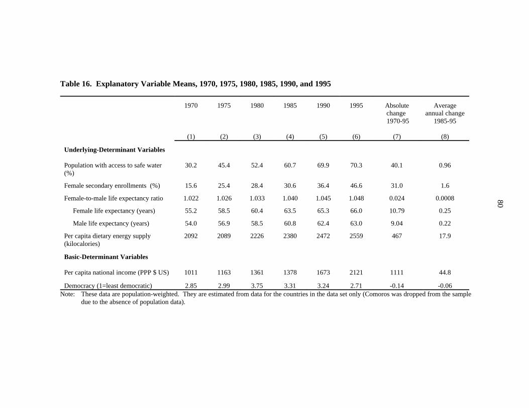
80
Table 16. Explanatory Variable Means, 1970, 1975, 1980, 1985, 1990, and 1995
1970 1975 1980 1985 1990 1995 Absolute Average
(1) (2) (3) (4) (5) (6) (7) (8)
change annual change 1970-95 1985-95
Underlying-Determinant Variables Population with access to safe water 30.2 45.4 52.4 60.7 69.9 70.3 40.1 0.96(%)
Female secondary enrollments (%) 15.6 25.4 28.4 30.6 36.4 46.6 31.0 1.6
Female-to-male life expectancy ratio 1.022 1.026 1.033 1.040 1.045 1.048 0.024 0.0008
Female life expectancy (years) 55.2 58.5 60.4 63.5 65.3 66.0 10.79 0.25
Male life expectancy (years) 54.0 56.9 58.5 60.8 62.4 63.0 9.04 0.22
Per capita dietary energy supply 2092 2089 2226 2380 2472 2559 467 17.9(kilocalories)
Basic-Determinant Variables
Per capita national income (PPP $ US) 1011 1163 1361 1378 1673 2121 1111 44.8
Democracy (1=least democratic) 2.85 2.99 3.75 3.31 3.24 2.71 -0.14 -0.06Note: These data are population-weighted. They are estimated from data for the countries in the data set only (Comoros was dropped from the sample
due to the absence of population data).

81
Table 17. Estimated Contributions of Underlying and Basic Determinants to Changes in the Prevalence of ChildMalnutrition by Region, 1970-1995
All Regions South Asia Africa East Asia North Africa the Caribbean(1) (2) (3) (4) (5) (6)
Sub-Saharan Near East and Latin America and
(percentage-point change in underweight rate)
Underlying Determinants
(1) Health environment -3.06 -4.56 -2.07 -2.74 -0.45 -1.80
(2) Quality of care for mothers and children
a) Women’s education -6.82 -4.61 -3.39 -9.27 -9.64 -6.98
b) Women’s relative status -1.84 -3.85 +1.27 -1.36 +0.28 -1.65
(3) National food availability (proxy for -4.14 -3.44 -0.048 -6.11 -2.34 -0.77 food securitya
(4) Total Percentage-Point Change -15.86 -16.46 -4.24 -19.48 -12.43 -11.20
Basic Determinantsb
(5) National Income -7.39a
(6) Democracy +0.18
(7) Total Percentage-Point Change -7.22
Notes: The estimates in this table are obtained by multiplying the coefficients on the proxy variables for each determinant (Table 8) by the change inthe proxy from 1970-1995. The changes are obtained from Appendix Tables A3-A7. The proxy for each determinant (identified by rownumber) is: (1) access to safe water; (2) female secondary enrollments; (3) female-to-male life expectancy ratio; (4) per capita dietary energysupply; (6) per capita gross domestic product; and (7) democracy index (see Table 3 for definitions of the variables).
These estimates take into account the changing coefficient on the variable as its level changes. a
As discussed in Section 5.2.3, the regression coefficients of the basic determinants model cannot be applied to the regions separately due tob
fundamental structural differences across the regions.

82
Table 18. 2020 Projections of the Prevalence and Numbers of Malnourished Children in Developing Countries,Alternative Scenarios
1995 in variable mean 1985-95
(1) (2)
Annual increase 2020 Scenarios
Status Quo Pessimistic Optimistic(3) (4) (5)
(1) Prevalence of child malnutrition (%) 31 -- 18.4 21.8 15.1
(2) Numbers of children malnourished (millions of under-fives) 167.1 -- 140.3 154.8 127.6
(3) Access to safe water 70.2 0.96 94.3 88.3 100percentage points
(4) Female secondary enrollments 46.6 1.60 86.7 76.7 96.7percentage points
(5) Female-to-male life expectancy ratio 1.047 0.00071 1.066 1.061 1.07
(6) Per capita dietary energy supply (DES) 2559 -- 2821 2662 2978
Notes: The estimates in rows (3) through (5) are based on 1985-95 average annual growth rates (column 2) calculated from the reported values of therespective variables given in columns (4) and (6) of Table 16. In the status quo scenario the rates are assumed to remain the same for theperiod 1995-2020. In the pessimistic scenario they are assumed to fall by 25%. In the optimistic scenario they are assumed to increase by25%. In the case that a variable hits its maximum, the estimated value for 2020 is replaced by the maximum. This is the case for the valuegiven for SAFEW in the optimistic scenario. The estimates for DES in row (6) are based on IFPRI IMPACT model projections as reported inRosegrant et al. (1995). The projections correspond to future developments in food prices, agricultural productivity, research investments,population growth and growth in nonagricultural incomes (see text for a full explanation).

83
Table 19. 2020 Projections of the Prevalence and Numbers of Malnourished Children in Developing Countries,Alternative Scenarios By Region
Percent Underweight Numbers underweight
Region 1995 2020 2020 2020 1995 2020 2020 2020Status Quo Pessimistic Optimistic Status Quo Pessimistic Optimistic
percent of under fives millions of under fives
South Asia 49.3 37.4 40.3 34.5 86.0 66.0 71.1 60.9
Sub-Saharan Africa 31.1 28.8 32.4 25.7 31.4 48.7 54.6 43.3
East Asia 22.9 12.8 13.1 12.6 38.2 21.4 21.9 20.9
Near East and North Africa 14.6 4.97 7.4 3.7 6.3 3.2 4.8 2.4
Latin America and the 9.5 1.92 4.0 0 5.2 1.1 2.3 0Caribbean
All Developing Countries 31.0 18.4 21.8 15.1 167.1 140.3 154.6 127.6
Notes: The estimates are based on projected future values of the underlying-determinant explanatory variables SAFEW, FEMSED,LFEXPRAT and DES defined in Table 3. Future values of the first three are based on 1985-95 average annual growth ratescalculated from the reported values of the respective variables given in columns (4) and (6) of Appendix Tables A3 through A7. In the status quo scenario the rates are assumed to remain the same for the period 1995-2020. In the pessimistic scenario they areassumed to fall by 25%. In the optimistic scenario they are assumed to increase by 25%. In the case that a variable hits itsmaximum, the estimated value for 2020 is replaced by the maximum. For South Asia this occurred for the variable SAFEW forall scenarios. For East Asia, it occurred for the variable FEMSED for all scenarios. For the Near East and North Africa itoccurred for SAFEW for all scenarios and for FEMSED for the optimistic scenario only. Projections of DES are based on IFPRIIMPACT model projections as reported in Rosegrant et al. (1995). They correspond to future developments in food prices,agricultural productivity, research investments, population growth and growth in nonagricultural incomes (see text for a fullexplanation).

84
Table 20. Strength of Impact of National Food Availability on Child Malnutrition: Country Groupings by High, Medium, and Low Impact
High Impact Medium Impact Low Impact (DES(DES less than 2300) (DES between 2300 and 3120) greater than 3120)a
South Asia Afghanistan, Bangladesh, Pakistan, India, MaldivesNepal, Sri Lanka
Sub- Ethiopia, Somalia, Eritrea, Cote d'Ivoire, Sudan, Benin,Saharan Burundi, Mozambique, Guinea-Bissau, Senegal,Africa Comoros, Congo-- Swaziland, Gabon, Nigeria,
Democratic Republic, Ghana, Mauritania, MauritiusCentral African Republic,Chad, Djibouti, Angola,Zambia, Niger, Zimbabwe,Madagascar, Kenya,Tanzania, Sierra Leone,Rwanda, Malawi, Liberia,Lesotho, Togo, Namibia,Congo, Guinea, Sao-Tomeand Principe, Mali,Cameroon, Burkina Faso,Botswana, Uganda, Gambia
East Asia Cambodia, Mongolia, Laos Thailand, Philippines, Korea-- South KoreaDP, Vietnam, Myanmar,China, Brunei, Malaysia,Macau, Indonesia
Near Yemen, Iraq Saudi Arabia, Jordan, Iran, Morocco, Libya,East/N. Kuwait, Algeria, Tunisia Egypt, Lebanon,Africa Syria, United Arab
Emirates, Cyprus,Turkey
Latin Haiti, Bolivia, Peru, Nicaragua, Dominican Mexico, BarbadosAmerica/ Guatemala Republic, Honduras, Cuba,Caribbean Venezuela, Ecuador, Guyana,
Panama, Bahamas, Paraguay,El Salvador, Surname, Jamaica,Trinidad and Tobago, Chili,Colombia, Uruguay, Belize,Costa Rica, Brazil, Dominica,Argentina
Notes: The country classifications are based on cutoffs determined by the two knots of a three-segmentlinear spline function for DES in a regression on underweight prevalence (see Table 8, column 3). The DES's are for 1995. The source is FAO (1998).
DES = Per capita Dietary Energy Supply measured in kilocalories.a

85Table 21. Comparison of the Strengths and Potential Impacts of the Determinants of Child Malnutrition (CHMAL)
1995 to reduce prevalence of percent of Percent Determinant malnutrition with increase inmean child malnutrition by 1 developing-country is below its desirable determinant to
(1) (2) (3) (4) (5)
Increase in variable needed Number in (2) as a Change in prevalence of child
percentage point range level (0-100 scale) desirable levela b c
Underlying Determinant Variables (percentage points)
South Asia (1995 CHMAL: 49.3%)Safe water (SAFEW) 79.7 13.1 13.2 -20.3 -1.6
Female secondary enrollments (FEMSED) 34.1 4.6 4.6 -65.9 -14.5
Female to male life expectancy ratio (LFEXPRAT) 1.023 0.0139 9.3 -58.9 -5.5
Per capita dietary energy supply (DES) 2356 94 4.5 -46.5 -3.9
Sub-Saharan Africa (1995 CHMAL: 31.1%) SAFEW 48.8 13.1 13.2 -51.2 -3.9
FEMSED 19 4.6 4.6 -81.0 -17.8
LFEXPRAT 1.054 0.0139 9.3 -35.2 -3.3
DES 2136 75 3.6 -60.2 -5.6
East Asia (1995 CHMAL: 22.9%) SAFEW 66.5 13.1 13.2 -33.5 -2.6
FEMSED 59.8 4.6 4.6 -40.2 -8.8
LFEXPRAT 1.0514 0.0139 9.3 -37.4 -3.5
DES 2720 188 9.0 -23.8 -2.1
Near East/Nth Africa (1995 CHMAL: 14.6%) (percentage points) SAFEW 81.5 13.1 13.2 -18.5 -1.4
FEMSED 57.9 4.6 4.6 -42.1 -9.2
LFEXPRAT 1.044 0.0139 9.3 -42.8 -4.0
DES 3172 333 16 +4.5 -0.7
Latin Am/Caribbean (1995 CHMAL: 9.5%) SAFEW 77.3 13.1 13.2 -22.7 -1.7
FEMSED 56.5 4.6 4.6 -43.5 -9.6
LFEXPRAT 1.098 0.0139 9.3 -1.9 -0.18
DES 2777 234 11.2 -20.2 -1.5
Basic Determinant Variablesd
Per capita national income 2121 202 9.7 -59.1 -18.5
Democracy 2.71 0.79 11.5 71.5 -5.5
Note: The table compares the relative strengths of the underlying determinants among one another and the basic determinants among one another. Since the two groups lie at differentlevels of causality, it is important not to compare the results for variables across the groups.
See Table 12 for variable ranges.a
The desirable levels of the variables are: SAFEW: 100%; FEMSED: 100%; LFEXPRAT: 1.1 (this is the average of the highest 20% of country-year data points in our sample in terms ofb
female-to-male life expectancy ratios [excluding the highest, which is 1.15 and far above the next highest, 1.12]); DES: 3100 (see text footnote for rationale); GDP: We set the desirablelevel at $4750. This is the level past which improvements in GDP per capita no longer contribute to reductions in child malnutrition (see Section 5.2.1.3); DEMOC: 7 (the maximumvalue of the index).These numbers are calculated using the regression coefficients in Table 8 columns (3) and (4). For DES and GDP, each group’s number is calculated using country averages (with thec
countries including all countries listed in Table A8--note: GDP will be expanded to all). Because the structural relationship between CHMAL and basic determinants differs by regions, we cannot provide reliable regional break downs. d

86
Table 22. Priorities by Region For Future Child Malnutrition Reduction (Underlying Determinants)
Region Rank of determinants by most potent impact Rank of determinants by most potential for Top Priorities on malnutrition relative to its existing range impact based on increases to desirable levels
(1) (2) (3)
South Asia 1. Food availability 1. Women's education 1. Food Availability2. Women's education 2. Women’s relative status 1. Women's education3. Women’s relative status 3. Food availability4. Health Environment 4. Health Environment
Sub-Saharan Africa 1. Food availability 1. Women's education 1. Food availability2. Women's education 2. Food availability 1. Women's education3. Women’s relative status 3. Health Environment 4. Health Environment 4. Women’s relative status
East Asia 1. Women's education 1. Women's education 1. Women's education2. Food Availability 2. Women’s relative status 2. Food Availability3. Women’s relative status 3. Health Environment 2. Women’s relative status4. Health Environment 4. Food availability
Near East and North 1. Women's education 1. Women's education 1. Women's educationAfrica 2. Women’s relative status 2. Women’s relative status 2. Women’s relative status
3. Health Environment 3. Health Environment 4. Food availability 4. Food availability
Latin America and the 1. Women's education 1. Women's education 1. Women's educationCaribbean 2. Women’s relative status 2. Health Environment 2. Women’s relative status
3. Food availability 3. Food Availability 2. Health Environment4. Health Environment 4. Women’s relative status
Notes: The rankings in column (1) are based on the numbers reported in Table 21, Column (3). The rankings in column (2) are based on the numbers reported in Table21, column (5). The top priorities in Column (3) are based on the highest ranked determinants in columns (1) and (2).

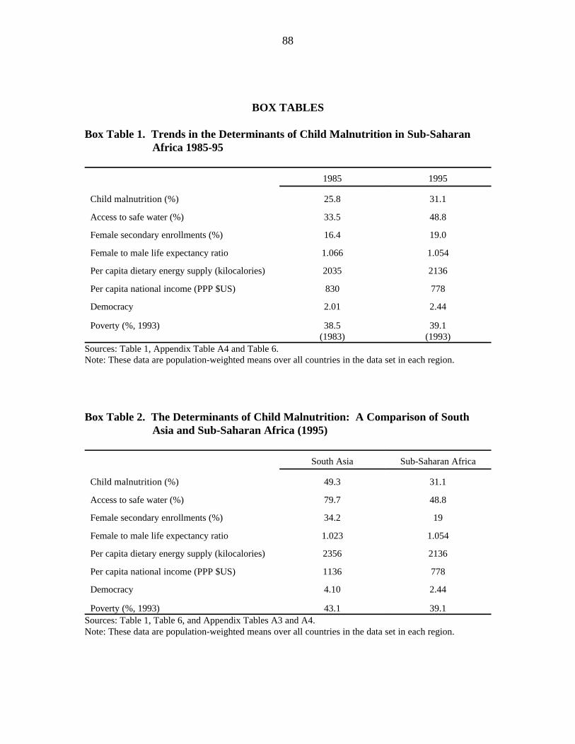
88
BOX TABLES
Box Table 1. Trends in the Determinants of Child Malnutrition in Sub-SaharanAfrica 1985-95
1985 1995
Child malnutrition (%) 25.8 31.1
Access to safe water (%) 33.5 48.8
Female secondary enrollments (%) 16.4 19.0
Female to male life expectancy ratio 1.066 1.054
Per capita dietary energy supply (kilocalories) 2035 2136
Per capita national income (PPP $US) 830 778
Democracy 2.01 2.44
Poverty (%, 1993) 38.5 39.1(1983) (1993)
Sources: Table 1, Appendix Table A4 and Table 6.Note: These data are population-weighted means over all countries in the data set in each region.
Box Table 2. The Determinants of Child Malnutrition: A Comparison of SouthAsia and Sub-Saharan Africa (1995)
South Asia Sub-Saharan Africa
Child malnutrition (%) 49.3 31.1
Access to safe water (%) 79.7 48.8
Female secondary enrollments (%) 34.2 19
Female to male life expectancy ratio 1.023 1.054
Per capita dietary energy supply (kilocalories) 2356 2136
Per capita national income (PPP $US) 1136 778
Democracy 4.10 2.44
Poverty (%, 1993) 43.1 39.1Sources: Table 1, Table 6, and Appendix Tables A3 and A4.Note: These data are population-weighted means over all countries in the data set in each region.


90
APPENDIX 1SUPPLEMENTARY TABLES


92
Table A1. Cross-Country Studies of the Determinants of Health Outcomes in Developing Countries
Study Variable Method countries Main Findings LimitationsDependent of
Number
Anand and Life expectancy, OLS 22 Per capita income loses its significance as an Limited list of dependent variables mayRavallion around 1985 explanatory variable once poverty and public cause omitted variable bias. Small sample(1993) spending on social services are controlled for. size. OLS estimation may lead to biased
estimates
Subbarao and Infant mortality, OLS 72 Female education (lagged 5 and 10 years) has OLS estimation may lead to biasedRaney (1995) 1985 a strong effect on IMR; access to family estimates. Mixed estimation of basic and
planning, pop. per physician, and GDP per underlying determinants only gives partialcapita are significant but not as effective. (rather than total) effect of basic
determinants.
Pritchett and Infant and child OLS, first- 58-111 Per capita GDP has a substantial positive Does not allow breakdown of theSummers mortality, life differences, (184- impact on infant and child health; education pathways through which average incomes(1996) expectancy, country fixed- 368) levels are also important. influence health outcomes. Since GDP
1960-1985 effects, and per capita facilitates educationalinstrumental investment, coefficient on GDP may notvariables. represent total income effect (biased downwards).
a
Notes: OLS = Ordinary least squares regression. Total number of observations.a

93
Table A2. Cross-Country Studies of the Determinants of Child Malnutrition in Developing Countries
Study Variable Method countries Main Conclusion LimitationsDependent of
Number
ACC/SCN Underweight OLS on pooled, 66 Energy availability, female education, public OLS estimation may give biased(1993) children, 1975- cross-section (100) expenditures on social services and size of the estimates.
1992 data child population under five all important
a
determinants; regional effects are statisticallysignificant (South Asia*kcal significant).
ACC/SCN Underweight Quasi first- 35 Growth in per capita income is an important Small sample size.(1994) children, 1975- differences (79) determinant.
1993
Gillespie, Change in Quasi first- 35 Growth in per capita income and (levels of) Mixture of levels and change variablesMason and prevalence of differences (# of public expenditures on health services are does not allow interpretation of coefficientMartorell underweight spells) significant determinants; energy availability estimates.(1996) children (1975- (levels and changes) is not significant.
1993)
Rosegrant et al. Underweight OLS on pooled, 61 Energy availability and social expenditures Use of predicted values from previous(1995) children cross-section (183) are significantly (negatively) associated with estimates means that significance and
1980-1990 data underweight rates, but female education and magnitude of parameter estimates areaccess to safe water are not. inaccurate.
Osmani Stunted OLS 45 Per capita income and female literacy are Inclusion of “low birthweight” variable in (1997) children, around important determinants of stunting; income estimating equation and OLS estimation
1990 distribution is not significant; low birthweight technique lead to biased parameteraccounts for South Asia's excessive estimates.malnutrition
Frongillo et al. Stunted and OLS 70 Energy availability, female literacy and per OLS estimation may give biased(1997) wasted children, capita GNP significant determinants; results parameter estimates. Mixed estimation of
post 1980 on health services differ by region. Female basic and underlying determinants onlyliteracy squared, immunization rates, military gives partial (rather than total) effect ofpopulation and energy availability (only for basic determinants.Asia) significant for wasting.
Notes: OLS = Ordinary least squares regression. Total number of observations.a

94
Table A3. Explanatory Variable Means (1970, 1975, 1980, 1985, 1990, and 1995),South Asia
1970 1975 1980 1985 1990 1995 1970-95(1) (2) (3) (4) (5) (6) (7)
AbsoluteChange
Population with access to safe water (%)19.8 39.3 50.5 53.7 80.9 79.7 +59.8
Female secondary enrollment rate (%)13.7 14.8 18.0 23.5 29.5 34.2 +21
Ratio of female life expectancy to malelife expectancy .970 .982 .992 1.00 1.014 1.023 +0.0537
Per capita dietary energy supply(kilocalories) 2105 1948 1975 2126 2264 2356 +251
Per capita gross domestic product (PPP$US) 674 682 724 768 962 1136 +461
Democracy index (1=least democratic) 5.17 5.17 5.48 4.83 5.24 4.10 -1.07Note: These data are population-weighted means over all countries in the data set in the region.
Table A4. Explanatory Variable Means (1970, 1975, 1980, 1985, 1990, and 1995)Sub-Saharan Africa
1970 1975 1980 1985 1990 1995 1970-95(1) (2) (3) (4) (5) (6) (7)
AbsoluteChange
Population with access to safe water (%) 21.6 26.6 29.8 33.5 42.9 48.8 +27.2
Female secondary enrollment rate (%) 3.6 6.5 10.6 16.4 15.8 19.0 +15.4
Ratio of female life expectancy to male 1.072 1.070 1.069 1.066 1.058 1.054 -0.0177life expectancy
Per capita dietary energy supply 2133 2083 2089 2035 2099 2136 +2.8(kilocalories)
Per capita gross domestic product (PPP 950 1000 963 830 851 778 -172$US)
Democracy index (1=least democratic) 2.26 2.45 3.10 2.01 2.13 2.44 +0.184Note: These data are population-weighted means over all countries in the data set in the region (excluding Comoros,
for whom population data are not available).

95
Table A5. Explanatory Variable Means (1970, 1975, 1980, 1985, 1990, and 1995),East Asia
1970 1975 1980 1985 1990 1995 1970-95(1) (2) (3) (4) (5) (6) (7)
AbsoluteChange
Population with access to safe water (%) 30.5 46.2 52.6 68.4 67.1 66.5 +35.9
Female secondary enrollment rate (%) 17.7 34.8 36.3 34.3 42.0 59.8 +42.2
Ratio of female life expectancy to male 1.032 1.032 1.038 1.048 1.051 1.051 +0.0189life expectancy
Per capita dietary energy supply 1998 2067 2280 2530 2618 2720 +722(kilocalories)
Per capita gross domestic product (PPP 628 739 938 1138 1582 2494 +1866$US)
Democracy index (1=least democratic) 1.37 1.46 2.58 2.19 1.59 1.34 -0.0317Note: These data are population-weighted means over all countries in the data set in the region.
Table A6. Explanatory Variable Means (1970, 1975, 1980, 1985, 1990, and 1995),Near East and North Africa
1970 1975 1980 1985 1990 1995 1970-95(1) (2) (3) (4) (5) (6) (7)
AbsoluteChange
Population with access to safe water (%) 75.6 67.8 72.2 67.9 81.9 81.5 +5.9
Female secondary enrollment rate (%) 14.1 21.4 31.1 43.3 54.6 57.9 +43.9
Ratio of female life expectancy to male 1.048 1.046 1.044 1.043 1.043 1.044 -0.004life expectancy
Per capita dietary energy supply 2265 2490 2804 2955 3097 3172 +907(kilocalories)
Per capita gross domestic product (PPP 1654 1932 2397 2462 2647 2653 +999$US)
Democracy index (1=least democratic) 2.07 2.73 3.06 3.35 3.52 2.09 +0.0219Note: These data are population-weighted means over all countries in the data set in the region.
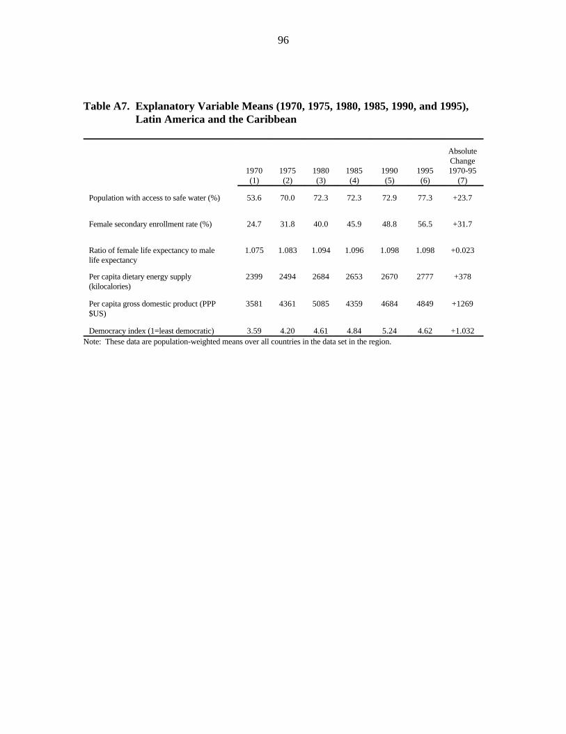
96
Table A7. Explanatory Variable Means (1970, 1975, 1980, 1985, 1990, and 1995),Latin America and the Caribbean
1970 1975 1980 1985 1990 1995 1970-95(1) (2) (3) (4) (5) (6) (7)
AbsoluteChange
Population with access to safe water (%) 53.6 70.0 72.3 72.3 72.9 77.3 +23.7
Female secondary enrollment rate (%) 24.7 31.8 40.0 45.9 48.8 56.5 +31.7
Ratio of female life expectancy to male 1.075 1.083 1.094 1.096 1.098 1.098 +0.023life expectancy
Per capita dietary energy supply 2399 2494 2684 2653 2670 2777 +378(kilocalories)
Per capita gross domestic product (PPP 3581 4361 5085 4359 4684 4849 +1269$US)
Democracy index (1=least democratic) 3.59 4.20 4.61 4.84 5.24 4.62 +1.032Note: These data are population-weighted means over all countries in the data set in the region.

97
Table A8. Regional Groupings of Developing Countries
Region Countries Countries
Numberof
South Asia 7 Afghanistan, Bangladesh, India, Maldives, Nepal, Pakistan, Sri Lanka
Sub-Saharan 45 Angola, Benin, Botswana, Burkina Faso, Burundi, Cameroon, CentralAfrica African Republic, Chad, Comoros, Congo, Congo--Democratic
Republic, Cote d'Ivoire, Djibouti, Eritrea, Ethiopia, Gabon, Gambia,Ghana, Guinea, Guinea-Bissau, Kenya, Lesotho, Liberia, Madagascar,Malawi, Mali, Mauritania, Mauritius, Mozambique, Namibia, Niger,Nigeria, Reunion, Rwanda, Sao-Tome and Principe, Senegal, SierraLeone, Somalia, Sudan, Swaziland, Tanzania, Togo, Uganda, Zambia,Zimbabwe
East Asia 14 Brunei, Cambodia, China, Indonesia, Korea--DP Republic, Loas,Macau, Malaysia, Mongolia, Myanmar, Philippines, South Korea,Thailand, Vietnam
Near East and 16 Algeria, Cyprus, Egypt, Iraq, Iran, Jordan, Kuwait, Lebanon, Libya,North Africa Morocco, Saudi Arabia, Syria, Tunisia, Turkey, United Arab Emirates,
Yemen
Latin America 28 Argentina, Bahamas, Barbados, Belize, Bolivia, Brazil, Chile,and the Colombia, Costa Rica, Cuba, Dominica, Dominican Republic, Ecuador,Caribbean El Salvador, Guatemala, Guyana, Haiti, Honduras, Jamaica, Mexico,
Nicaragua, Panama, Paraguay, Peru, Suriname, Trinidad and Tobago, Uruguay, Venezuela
TOTAL 110
Note: The regional classification of countries corresponds to that employed for IMPACT modelprojections.

FIGURES
(Available from authors)

99
BOX FIGURE
(Available from authors)

APPENDIX 2DATA AND SOURCES
(Available from authors)

REFERENCES
Ahooja-Patel, Krishna (1993). "Gender Distance Among Countries." Economic and
Political Weekly. February 13, pp. 295-305.
Alexandratos, Nikos, ed. (1995). World Agriculture Toward 2010: An FAO Study.
Rome: Food and Agriculture Organization of the United Nations, and Chichester:
John Wiley and Sons.
Anand, Sudhir, and Martin Ravallion (1993). “Human Development in Poor Countries:
On the Role of Private Incomes and Public Services.” Journal of Economic
Perspectives. Vol. 7, No. 1, pp. 133-150.
Baltaji, Badi H. (1995). Econometric Analysis of Panel Data. Chichester: John Wiley
and Sons.
Behrman, Jere R., and Anil B. Deolalikar (1988). “Health and Nutrition.” In Handbook
of Development Economics, Vol. 3, ed. H. Chenery and T. N. Srinivasan.
Amsterdam: North-Holland.
Bidani, Benu, and Martin Ravallion (1997). “Decomposing Social Indicators Using
Distributional Data.” Journal of Econometrics. Vol. 77, pp. 125-139.
Bound, John, David A. Jaeger, and Regina M. Baker (1995). “Problems with
Instrumental Variables Estimation When the Correlation Between the Instruments
and the Endogenous Explanatory Variable is Weak." Journal of the American
Statistical Association. Vol. 90, No. 430, pp. 443-450.
Brown, Lynn (1996). The Potential Impact of AIDS on Population and Economic
Growth Rates. Food, Agriculture, and the Environment Discussion Paper No. 15.
Washington, D.C.: International Food Policy Research Institute.
Davidson, Russell, and James G. Mackinnon (1993). Estimation and Inference in
Econometrics. New York: Oxford University Press.
Deaton, Angus (1997). The Analysis of Household Surveys: A Microeconometric
Approach to Development Policy. Baltimore, Md., U.S.A.: Johns Hopkins
University Press.
Deininger, Claus, and Lyn Squire (1996). "A New Data Set Measuring Income
Inequality." The World Bank Economic Review. Vol. 10, No. 3, pp. 565-91.
Drèze, J., and Amartya Sen, eds. (1989). Hunger and Public Action. New York: Oxford
University Press.
Engle, Patrice, Purnima Menon, and Lawrence Haddad (1997). Care and Nutrition:
Concepts and Measurement. Washington, D.C.: International Food Policy
Research Institute.
FAO (Food and Agriculture Organization of the United Nations) (1996). The Sixth World
Food Survey. Rome.

102
FAO (Food and Agriculture Organization of the United Nations) (1998). The FAOSTAT
database. This database can be accessed through the United Nations Food and
Agriculture Organization home page at http://apps.fao.org/cgi-bin/nph-db.pl.
Frankenberger, Timothy R. (1996). “Measuring Household Livelihood Security: An
Approach for Reducing Absolute Poverty." Food Forum. No. 34 (November-
December 1996). Washington, D.C.: Food Aid Management.
Freedom House (1997). Freedom House democracy data can be requested at the
following email address: [email protected].
Frongillo, Edward A., Mercedes de Onis, and Kathleen M.P. Hanson (1997).
“Socioeconomic and Demographic Factors Are Associated with Worldwide
Patterns of Stunting and Wasting of Children.” Journal of Nutrition. December.
Gillespie, Stuart, John Mason, and Reynaldo Martorell. 1996. How Nutrition Improves.
UN ACC/SCN State-of-the-Art Series Nutrition Policy Discussion Paper No. 15.
Geneva: United Nations, Administrative Committee on Coordination/
Subcommittee on Nutrition.
Green, W. H. (1997). Econometric Analysis. Third edition. New York: Macmillan.
Haddad, Lawrence, and Arne Oshaug (1998). "How Does the Human Rights Perspective
Help to Shape the Food and Nutrition Policy Research Agenda?" Food Policy.
Vol. 23, No. 5, pp. 329-346.
Haddad, Lawrence, John Hoddinott, and Harold Alderman, eds. (1997). Intrahousehold
Resource Allocation in Developing Countries: Models, Methods and Policy.
Baltimore, Md., U.S.A.: The Johns Hopkins University Press.
Haddad, Lawrence, Patrick Webb, and Alison Slack (1997). "Trouble Down on the
Farm: What Role of Agriculture in Meeting 'Food Needs' in the Next 20 Years?"
International Food Policy Research Institute, Washington, D.C. Photocopied.
Haddad, Lawrence, Saroj Bhattarai, Maarten Immink, and Shubh Kumar (1996).
Managing Interactions Between Household Food Security and Preschooler Health.
Food, Agriculture, and the Environment Discussion Paper No. 16. Washington,
D.C.: International Food Policy Research Institute.
Haddad, L., M. D. Westbrook, D. Driscoll, E. Payongayong, J. Rozen, and M. Weeks
(1995). Strengthening Policy Analysis: Econometric Tests Using Microcomputer
Software. Microcomputers in Policy Research 2. Washington, D.C.: International
Food Policy Research Institute.
103
Hoddinott (1997). "Water, Health, and Income: A Review." Food Consumption and
Nutrition Division Discussion Paper No. 25. International Food Policy Research
Institute, Washington, D.C.
ICN (International Conference on Nutrition) (1992). Caring for the Socio-Economically
Deprived and Nutritionally Vulnerable. Major Issues for Nutrition Strategies
Theme Paper # 3. ICN/92/INF/7. Rome: Food and Agriculture Organization of the
United Nations/World Health Organization.
Isham, J., D. Narayan, and L. Pritchett (1995). “Does Participation Improve
Performance? Establishing Causality with Subjective Data.” World Bank Economic
Review. Vol. 9, No. 2, pp. 175-200.
Kahn, Harold A., and Christopher T. Sempos (1989). Statistical Methods in
Epidemiology. Oxford: Oxford University Press.
Kishor, Sunita, and Katherine Neitzel (1996). “The Status of Women: Indicators for
Twenty-Five Countries.” Demographic and Health Surveys Comparative Studies
No. 21. Calverton, Md., U.S.A.: Macro International, Inc.
Martorell, Reynaldo (1997). "Undernutrition During Pregnancy and Early Childhood:
Consequences for Cognitive and Behavioral Development." In M. D. Young, ed.
Early Child Development: Investing in Our Children's Future. New York: Elsevier
Science.
Martorell, Reynaldo, U. Ramakrishnan, D. G. Schroeder, P. Melgar, and L. Neufeld
(1998). “Intrauterine Growth Retardation, Body Size, Body Composition and
Physical Performance in Adolescence.” European Journal of Clinical Nutrition.
Vol. 51, No. S1, pp. S43-S53.
Messer, Ellen, Marc J. Cohen, and Jashinta D'Costa (1998). Food from Peace: Breaking
the Links Between Hunger and Conflict. Food, Agriculture, and the Environment
Discussion Paper No. 24. Washington, D.C.: International Food Policy Research
Institute.
Mohiuddin, Yasmeen (1996). "Country Rankings By the Status of Women Index." Paper
presented at the 1996 Conference of the International Association for Feminist
Economics.
Oshaug, Arne, Wenche Barth Eide, and Asbjørn Eide (1994). "Human Rights: A
Normative Basis for Food and Nutrition-Relevant Policies." Food Policy. Vol. 19,
No. 6, pp. 491-516.
Osmani, S. R. (1997). “Poverty and Nutrition in South Asia.” Text of the Abraham
Horwitz lecture. Chapter 3 in Nutrition and Poverty. Papers from the UN

104
ACC/SCN 24th Session Symposium, Kathmandu. Nutrition Policy Paper #16, pp.
23-51.
Penn World Tables (1992).
Pritchett, Lant, and Lawrence H. Summers (1996). “Wealthier is Healthier.” Journal of
Human Resources. Vol. 31, No. 4, pp. 841-868.
Przeworski, A., and F. Limongi (1993). “Political Regimes and Economic Growth.”
Journal of Economic Perspectives. Vol. 7, No. 3, pp. 51-69.
Quisumbing, Agnes, Lynn Brown, Hilary Sims Feldstein, Lawrence Haddad, and
Christine Pena (1995). Women: The Key to Food Security. Washington D.C.:
International Food Policy Research Institute.
Ramakrishnan, U., J. Rivera, and R. Martorell (1998, in press). “A Critical Review of the
Relationship Between Micronutrient Malnutrition and Pregnancy Outcomes.”
Nutrition Research.
Ramalingaswami, Vulimiri, Urban Johnsson, and Jon Rohde (1996). "The Asian
Enigma." In Progress of Nations. New York: United Nations Children's Fund.
Ravallion, Martin, and Shaohua Chen (1996). "What Can New Survey Data Tell Us
about Recent Changes in Distribution and Poverty?" World Bank Policy Research
Department. Washington, D.C. Photocopied.
River, Juan, Mario Flores, Reynaldo Martorell, Usha Ramakrishnan, and Paul Melgar
(1996). "Generational Effects of Supplementary Feeding During Early Childhood."
In F. Battaglia et al. (eds.), Maternal and Extrauterine Factors. Their Influence on
Fetal and Infant Growth, pp. 197-204. Fifth International Workshop. Universidad
de Salamanca, Spain. Madrid: Ediciones Ergon.
Roemer, Michael, and Mary Kay Gugerty (1997). Does Economic Growth Reduce
Poverty? CAER II Discussion Paper No. 4. Cambridge, Mass., U.S.A.: Harvard
Institute for International Development.
Rosegrant, Mark W., Mercedita Agcaoili-Sombilla, and Nicostrato D. Perez (1995).
Global Food Projections to 2020: Implications for Investment. Food, Agriculture,
and the Environment Discussion Paper No. 5. 2020 Vision. Washington, D.C.:
International Food Policy Research Institute.
Ryan, Joseph E. (1995). "The Comparative Survey of Freedom—1994-1995 Survey
Methodology." In Adrain Karatnycky, Kathleen Cavanaugh, James Finn, Charles
Graybow, Douglas W. Payne, Joseph E. Ryan, Leonard R. Sussman, and George
Zarychy, eds. Freedom in the World: The Annual Survey of Political Rights and

105
Civil Liberties 1994-1995. Lanham, Md., U.S.A.: University Press of America,
Inc.
Sala-I-Martin, Xavier X. (1997). "I Just Ran Two Million Regressions." American
Journal of Agricultural Economics. Vol. 87, No. 2, pp. 178-183.
Sen, Amartya (1998). “Mortality as an Indicator of Economic Success and Failure.”
Economic Journal. Vol. 28, pp. 1-25.
Smith, Lisa C. (1998a). “Macroeconomic Adjustment and the Balance of Bargaining
Power in Rural West African Households.” Presented at the American Agricultural
Economics Association Annual Meetings, Salt Lake City, Utah, August.
Smith, Lisa C. (1998b, forthcoming). “Can FAO’s Measure of Chronic
Undernourishment Be Strengthened?” Food Policy. Vol. 23, No. 4.
Smith, Lisa C., and Jean-Paul Chavas (1997). “Commercialization and the Balance of
Women’s Dual Roles in Non-Income-Pooling West African Households.”
American Journal of Agricultural Economics. Vol. 79, pp. 589-594.
Smith, Lisa C., Amani El Obeid, Helen H. Jensen, and Stanley R. Johnson (1998,
forthcoming). "The Geography and Causality of Food Insecurity in Developing
Countries." Chapter 5 in Stanley R. Johnson, Amani El Obeid, Helen H. Jensen,
and Lisa C. Smith, eds. Food Security: New Solutions for the 21st Century. Ames,
Iowa: Iowa State University Press.
SPSS (1993). SPSS for Windows Release 6.0 Help Facility. SPSS Inc.
Subbarao, K., and Laura Raney (1995). “Social Gains from Female Education: A Cross-
National Study.” Economic Development and Cultural Change. Vol. 44, No. 1, pp.
105–128.
UN ACC/SCN (United Nations, Administrative Committee on Coordination/
Subcommittee on Nutrition) (1992). Second Report on the World Nutrition
Situation. Volume I. Geneva.
UN ACC/SCN (United Nations, Administrative Committee on Coordination/
Subcommittee on Nutrition) (1993). Second Report on the World Nutrition
Situation. Volume II. Geneva.
UN ACC/SCN (United Nations, Administrative Committee on Coordination/
Subcommittee on Nutrition) (1994). Update on the Nutrition Situation, 1994.
Geneva.
UN ACC/SCN (United Nations, Administrative Committee on Coordination/
Subcommittee on Nutrition) (1996). Update on the Nutrition Situation, 1996.
Geneva.

106
UN ACC/SCN (United Nations, Administrative Committee on Coordination/
Subcommittee on Nutrition) (1997). Third World Report on the Nutrition Situation.
Geneva.
UNDP (United Nations Development Programme) (1992). Human Development Report
1992. New York: Oxford University Press.
UNDP (United Nations Development Programme) (1997). Human Development Report
1997. New York: Oxford University Press.
UNESCO (United Nations Educational, Scientific and Cultural Organization) (1998).
UNESCOSTAT Database. The database can be accessed through UNESCO's home
page at http://unescostat.unesco.org.
UNICEF (United Nations Children's Fund) (1990). "Strategy for Improved Nutrition of
Children and Women in Developing Countries." New York.
UNICEF (United Nations Children's Fund) (1986–1988). The State of the World's
Children 1986. New York.
UNICEF (United Nations Children's Fund) (1990–1992). The State of the World's
Children 1990. New York.
UNICEF (United Nations Children's Fund) (1994–1998). The State of the World's
Children 1994. New York.
Victora, Cesar G. (1992). “The Association Between Wasting and Stunting: An
International Perspective.” Journal of Nutrition. Vol. 122, pp. 1105–1110.
WHO (World Health Organization) (1996). Water Supply and Sanitation Sector
Monitoring Report 1996. WHO Document # WHO/EOS/96.15. Geneva.
WHO (World Health Organization) (1997). WHO Global Database on Child Growth
and Malnutrition. Programme of Nutrition. WHO Document # WHO/NUT/97.4.
Geneva.
World Bank (1986). Poverty and Hunger: Issues and Options for Food Security in
Developing Countries. Washington, D.C.
World Bank (1997a and 1998a). World Development Indicators on CD-Rom.
Washington, D.C.
World Bank (1997b and 1998b). World Development Indicators. Washington, D.C.
WRI (World Resources Institute) (1986). World Resources 1986. Oxford: Oxford
University Press.
WRI (World Resources Institute) (1987). World Resources 1987. Oxford: Oxford
University Press.

107
WRI (World Resources Institute) (1988). World Resources 1988-89. Oxford: Oxford
University Press.
WRI (World Resources Institute) (1990). World Resources 1990-91. Oxford: Oxford
University Press.
WRI (World Resources Institute) (1992). World Resources 1992-93. Oxford: Oxford
University Press.
WRI (World Resources Institute) (1994). World Resources 1994-95. Oxford: Oxford
University Press.
WRI (World Resources Institute) (1996). World Resources 1996-97. Oxford: Oxford
University Press.