Experiments in Political Economy1

Thomas R. Palfrey2

July 8, 2014

1This was prepared for publication as a chapter in The Handbook of Experimental Economics,Volume 2, edited by John Kagel and Alvin Roth. The financial support of the National ScienceFoundation and the Gordon and Betty Moore Foundation is gratefully acknowledged. I wish tothank many coauthors and colleagues for sharing their insights about laboratory experimentationin political science and game theory. John Kagel, Aniol Llorente-Saguer, Rebecca Morton, KirillPogorelskiy, and Rick Wilson provided many helpful comments and advice on earlier drafts of thesurvey. I am especially indebted to Richard McKelvey, Charles Plott, and Howard Rosenthal,who were instrumental in shaping my own research in this area. None of them are responsible forany shortcomings in the final product. Parts of this chapter expand on material from previoussurveys and lectures by the author.

2Division of the Humanities and Social Sciences, California Institute of Technology, Pasadena,CA, USA,91125. trp@hss.caltech.edu

1 Introduction and Overview

The biggest challenge to writing a survey about experiments in political economy is an-

swering the question: What is political economy? This being the information age, the

natural first step was to google ”political economy”. This produced the following remark-

ably broad definitions of the topic.

According to Wikipedia1, ”Political Economy refers to different, but related, ap-

proaches to studying economic and related behaviors, ranging from the combination of

economics with other fields, to using different fundamental assumptions which challenge

orthodox economic assumptions.” The source then goes on to list several completely dif-

ferent subdefinitions of the term, followed by an even longer list of disciplines which relate

to political economy: sociology; political science; anthropology; psychology; history; eco-

nomics; law; human geography; ecology; international relations; cultural studies; and

communication.

To narrow things somewhat, the field ”Positive Political Economy” seems to encom-

pass everything (and more) that pertains to laboratory experiments in the economics

tradition. It is the title of at least two books, and focuses on the kinds of issues and

methodologies most familiar to modern-day economists.2 However, even this does not

help much in narrowing the scope of this survey. According to one of the Cambridge

University Press webpages,3 ”Positive Political Economy investigates how observed dif-

ferences in institutions affect political and economic outcomes in various social, economic,

and political systems.” If one opens up the book, it turns out to be a collection of essays

on various topics in macroeconomics and econometrics. Given that the present volume

already includes a chapter on experiments related to macroeconomics, I will exclude that

brand of ” political economy” experiment from this survey.

Clearly the subject matter, ”Political Economy”, defines an area of study that encom-

passes several fields of economics, overlaps with several other disciplines, and is also a

major field of study by political scientists (Wikipedia’s omission from related disciplines

notwithstanding).

So, now that we have slightly narrowed the topic, the practical question is where

to start and where to stop? First, rather than thinking like an economist and looking

at economics experiments that are related to political economy issues, I have chosen the

”political” half of political economy as the starting point. There is no chapter in either this

1http://en.wikipedia.org/wiki/Political economy November 18, 2013.2See Alt and Shepsle (1990). It is also the title of a monograph series published by Routledge.3http://www.cambridge.org/us/catalogue/print.asp?isbn=9780521572156&print=y

1

or the previous edition of the volume that covers political science experiments. Yet, some

of the chapters, most notably the chapter on public goods (Ledyard 1996), cover material

that could easily be categorized as political science; some of the seminal contributions

in these areas were made by political scientists, explicitly with application to political

science in mind.4

To make the survey manageable, I have further limited the scope considerably in

three ways. First, I have excluded from consideration all non-incentivized experiments in

political science and political economy. To give an idea of how much this leaves out, in an

earlier volume coauthored with Donald Kinder (Kinder and Palfrey 1993), we devoted fully

one-half of the book to nonincentivized experiments, and the other half to incentivized

experiments, ”in the economics tradition.” This exclusion is not meant to demean that

literature nor to suggest that it lies on a lower intellectual plane. It is excluded mainly

for compatibility of this chapter with the rest of the chapters of the handbook.5 Those

experiments are in the psychology tradition, and the experiments I will be discussing all

fall clearly in the economics tradition, at least methodologically.

Second, I exclude field experiments and economics-style experiments conducted in a

field setting, focusing exclusively on controlled laboratory experiments. An obvious reason

is that the basic methodology of field experiments is fundamentally different. Neither the

degree of control nor the ease of replicability that distinguish laboratory settings is there.

These experiments also have the feature that the level of intrusion into the lives of the

subjects is much greater than in economics-style experiments,6 and this raises a different

and more complicated set of issues, both logistical and ethical. Another reason why I have

excluded field experiments is that I have never conducted any such experiments myself,

and therefore am only qualified to judge the contributions of this work as an interested

outsider rather than a true expert. This reflects a respect for the difficulties inherent

in and skills required for field experimentation. Just as someone who has never run

an economics or political science experiment in the laboratory is ill-equipped to reliably

judge the quality of a paper in that field, someone who has never been involved in a field

experiment is poorly equipped to write a survey on it.

Third, I will not include public goods experiments as a special section of this survey.

John Ledyard already contributed an excellent one to the previous edition, and there is

a chapter in the current volume as well. There will be some passing discussion of public

4This includes work by the recent Nobel prize winning political scientist, Eleanor Ostrom.5An exception is the chapter in the previous edition, concerning individual choice experiments

(Camerer 1996).6This may be changing somewhat in laboratory experiments, as experimenters attempt to scale up

the mini-economies and mini-polities being studied.

2

goods experiments, however, where appropriate.

This leaves us with a subset of the laboratory research in positive political science, a

small bite from the political economy beast.

1.1 Methodology: Relationship to experimental economics

This survey also focuses exclusively on experiments that follow the style pioneered in ex-

perimental economics several decades ago by by Vernon Smith: incentivized, controlled,

laboratory experiments. The analogy between this style of political science experimen-

tation and economics experimentation reflect the close intellectual heritage shared by

economic theory, formal political theory, and political economy – a heritage whose over-

lap can be seen in the ideas and seminal contributions of Condorcet, Cournot, and Adam

Smith, carrying forward to the more familiar modern contributions of Kenneth Arrow,

Duncan Black, William Riker, and others.

The shared connection with rigorous theory is not only due to a long heritage of shared

ideas and research questions, but is also reflected in the birth of laboratory investigations

in economics and political science. The pioneering researchers in the laboratory in both

disciplines were trained primarily as theorists who became mainly interested in learn-

ing whether the theories were reliable, or curious about environments where theory gave

little guidance. They turned to laboratory experiments to test theory, in the grand tradi-

tion of the physical and natural sciences. In those other disciplines, scientists undertook

laboratory experiments, not because there was no field data (indeed field observation is

also important in physics, geology, and biology), but because laboratories opened up new

questions for which field data was either unavailable or inadequate.

Laboratory experiments in economics designed for theory testing have three key fea-

tures. First, such experiments create real, but isolated, environments, which operate under

a set of institutional rules that are highly controlled and specifically designed to address

the research questions of an experimenter. Second, the participants of these experiments

are given incentives that are consistent with the theoretical structure of preferences and

technology that is present in the theoretical models. For example, in market experiments

the incentives are designed to induce demand and supply functions. Third, an effort is

usually made to avoid specific contexts that could confound the incentive structure. For

example, in market experiments the participants buy and sell abstract things, as opposed

to labeling the items as ”hair spray”, ”broccoli” or some other real commodity. The pre-

dictions of these theories about behavior in the controlled environment were quantified

3

and the results of the experiment therefore provided a direct test of the theory.7

One of the pioneers of political science experiments in the economics tradition is

Charles Plott. He conducted early market experiments, as well, to compare the effects

of different ways of organizing markets in terms of the detailed rules governing trade

and exchange,8 but his initial forays in the laboratory were in political science in the

early 1970s, and the institutional focus of his early experiments had its foundation in

social choice theory. Plott had the insight that in principle one could apply induced-value

methods to study and compare the effect of different political institutions and voting

rules on committee decisions and policy outcomes, although the specific implementation

required some innovative techniques. The use of formal theoretical modeling in political

science (”positive political theory”) and social choice theory was developing rapidly at the

same time, and these theories were similar to economic theories in the sense that they were

deeply rooted in the basic concepts of incentives, rational choice, and equilibrium. The

models generated precise quantitative testable predictions about behavior and outcomes in

non-market settings such as committees, elections, courts, bureaucracies, and legislatures.

The nature of institutions being studied is somewhat different in political science than in

economics, but both disciplines are concerned with basic questions of resource allocation,

mechanism design, efficiency, and distribution. Both have quantitative units of account

that determine these allocation decisions. In political science, the score is kept with

votes; in economics, the unit of account is monetary. The existence of these quantitative

accounting methods in both disciplines naturally lends itself to mathematical analysis.

And the rigorous theory developed with such mathematical analysis permits the precise

formulation and statement of hypotheses and predictions that are amenable to testing in

the laboratory. The quantitative perspective is also useful, as it is in the sciences, to make

precise observational statements and measurements (national income, margin of victory,

etc.) even in the absence of theory. Pure observation, measurement, and laboratory data

together provide the fodder for new theory.

Experimentation using controlled, incentivized, context-free environments naturally

followed rather than preceded such research in economics. At the time economists began to

design and conduct laboratory experiments with markets and games in the 1950s, rigorous

theory as we think of it in economics was virtually nonexistent in political science. The

development of a rigorous and quantitative theoretical approach to the study of politics –

social choice theory and positive political theory – was virtually a prerequisite for this style

7A fourth feature of experiments in the economics tradition is the absence of deception, which is alsogenerally the case in incentivized political science experiments.

8See, for example, Plott and Smith (1978),.

4

of laboratory research in political science. More recently, as research in positive political

theory and political applications of game theory is maturing and having an impact in

all subfields of political science, the experimental playing field for political scientists is

rapidly expanding.

1.2 Chapter road map

The focus of this chapter will be on political economy experiments that can be loosely

organized around five different categories, and all are tightly linked to formal theoretical

modeling in political science. The goal is not to discuss every experimental paper on

every topic in political economy – that would require a book – rather, to identify the

main insights and tentative conclusions of the most important of these experiments. The

frontiers of research in political economy experimentation have been moving rapidly, and

this survey will attempt to give a snapshot of this frontier at one point in time. They

five topics are: (1) committee bargaining; (2) elections and candidate competition; (3)

voter turnout; (4) information aggregation in committees; (5) voting methods that reflect

preference intensity.

The pioneering experiments in political economy studied basic principles of commit-

tee and voting behavior that had been developed in the axiomatic social choice theory

literature in the 1950s and 1960s. The aim was a study of the fundamental properties of

majority rule, and to gather scientific evidence about how actual behavior in committees

compared to these abstract theoretical constructs. A key question asked was whether

Condorcet winners, when they exist, become the outcomes of committee decision making

under majority rule. If so, why? If not, when does it fail and why? The social choice

literature was almost entirely normative at the time (1970s), with essentially no empirical

component at all.

To scholars well-versed in political economy and social choice theory, these questions

almost seemed too obvious a point to merit empirical investigation, but it turned to be a

much more difficult question to address, including the thorny problem of specifying exactly

what it means for a committee to operate under majority rule. There are many possible

procedures governing the proposing and seconding of motions, discussion, recognition,

amendments, adjournment, and so forth. A complete description of these is a daunting

task.9 Running an experiment to investigate the effect of procedures on outcomes forces

the experimenter to define in very precise terms the specific rules that the laboratory

9The most recent edition of Robert’s Rules of Order (2011) rambles on for more than 800 dense pages.Robert’s Rules for Dummies (2004) is 360 pages long.

5

committees had to follow. These rules may then be tweaked in subtle ways to address

questions of robustness and comparative statics.

This is comparable to the early experiments to study the law of supply and demand

in economics, when ”competitive markets” were implemented. What does ”competitive

market” mean in terms of the details of how the market is to be organized? For example,

is it organized a double auction or a one-sided auction? Is there a centralized open book

or do trades go through a market maker instead? Do trades clear continuously or is it

organized as a call market?

In committee experiments there are similar choices to make about majority rule pro-

cedures that had to be faced. What does ”majority rule” mean in terms of the details of

committee procedures? How are proposals made? Is there a chair of the committee who

has the power of recognition? How can amendments be made? Is there an open or closed

rule? Such questions are endless!

Not surprisingly, it turns out that for both kinds of experiments – committee exper-

iments and market experiments – the performance of abstract mathematical theories to

predict behavior sometimes worked well and sometimes did not, and this variance in per-

formance depended on both environmental parameters (preferences, feasible alternatives,

technology, etc.) and institutional parameters and details.10 This dependence suggested

that the axiomatic theories, which largely abstracted from institutional details, needed to

be reformulated in a way that incorporated such details as procedural rules into the formal

theoretical structure in order to obtain empirically valid and robust theoretical results.

One could easily argue that laboratory experiments in political economy provided the

first non-circumstantial evidence that institutions matter in committee decision making.

This evidence was not only non-circumstantial but also had the benefit of being replicable

and relatively easy to check for robustness. The theory offered precise comparative static

tests about how changing the environment or institution leads to changes in committee

outcomes. These effects were causal, because the environment and institutional details in

a laboratory experiment are clearly exogenous, unlike, say, comparisons between different

political systems based on historical data. This allows for much stronger claims about

cause and effect, as opposed to simple correlations between preferences, institutions, and

outcomes.

In the next section we discuss experiments coming out of two rather different ap-

proaches to the investigation of committee bargaining procedures and decision making.

First we try to clarify the main findings and explore in further detail results from the

10Many of these solution concepts came from cooperative game theory – for example the bargainingset and the von Neumann Morgenstern solution.

6

initial wave of political economy experiments based on axiomatic social choice theory and

cooperative game theory. Second, we will explore the much more recent experiments on

committee bargaining that are designed to test theories from noncooperative game theory.

Noncooperative game theory, by specifying the institutional details as ”rules of a game”,

often makes more precise predictions about institutional effects than the axiomatic ap-

proach. Many of the experiments discussed in later sections, including most political

economy experiments of the last two decades, will also be out of the noncooperative game

theory tradition. In the next section, the main focus is on noncooperative game theo-

retic models of committee decision making in a distributive politics (divide-the-dollar)

setting where Condorcet winners do not exist. These are constant sum games, which

are in stark contrast to the earlier focus on non-constant sum environments such as the

Downs-Hotelling spatial model where preferences were often specified so that a majority

rule core existed. These noncooperative bargaining models also differ from the axiomatic

ones by specifying details of the dynamics and timing of procedures and strategies. The

axiomatic models were completely static in nature.

Section three explores an important second wave of laboratory experiments in politi-

cal economy, which followed on the heels of the committee bargaining studies of majority

rule. This second wave was also interested in the empirical properties of majority rule

institutions, but focused on competitive elections and candidate competition rather than

committee bargaining. There is a range of questions addressed by these electoral compe-

tition experiments, and most of these are also central questions that have been studied

in more traditional empirical political science. In particular, we will focus on the follow-

ing four topics: retrospective voting; testing the median voter theorem about candidate

platform convergence in winner-take-all majority-rule elections; the effect of polls as coor-

dinating devices for voters and information aggregation in elections with more than two

candidates; and the effect of candidate quality on candidate divergence.

Section four investigates a different set of research questions related to questions of

political participation, especially voter turnout. The study of political participation has

close theoretical links with related questions about public good provision, free riding, and

coordination games. This section will highlight some of the connections between findings

in voter turnout experiments and the insights and regularities from related game theoretic

experiments on entry, coordination, and threshold public goods.

Section five examines several recent experiments on the effects of voting rules and pro-

cedures on information aggregation in committees. For the last decade, there has been a

surge of theoretical research addressing questions of efficiency and information aggregation

7

by voting. This new literature has its roots in questions originally posed and analyzed by

Condorcet in the 18th century, and is now commonly referred to as The Condorcet Jury

Problem. Each person in a committee (or electorate) has a piece of information about a

true state of the world, and the committee is choosing a decision, where the best decision

depends on the state of the world. One can think of this dispersed information as hunches

or intuitions, or even different interpretations of the same data. From a theoretical anal-

ysis based on noncooperative game theory, one can show that different voting rules and

procedures can have different information aggregating properties. For example, different

outcomes are predicted under majority and unanimity rules; this varies in surprising ways

with the size of the committee, and also depends on whether voting takes place simulta-

neously or sequentially. Most of the laboratory studies of information aggregation look at

environments where there is no preference aggregation problem: that is, all voters have

the same (state-contingent) preferences, but differ only in their information.

Section six summarizes results from experiments that examine theoretical models of

voting procedures that are explicitly designed for environments where intensity of prefer-

ence plays an important role. This includes experiments that address traditional questions

of interest in political economy, such as logrolling and vote trading, as well as the design

and performance of more novel specialized voting procedures such as storable votes and

qualitative voting.

2 Experiments in Committee bargaining

This section has two subsections: (i) early experiments from the axiomatic social choice

theory tradition, which focus on the core of majority rule games and related concepts

from cooperative game theory; and (ii) more recent laboratory studies of bargaining in

committees with much more structured rules about proposal-making and voting – rules

that are sufficiently simple to be studied as well-defined extensive form games.

2.1 Unstructured committee bargaining

This line of research, beginning with the landmark article by Fiorina and Plott (1978),

explores two distinctly different kinds of questions. First, it tests the basic theory of the

core in small committees, and examines its robustness with respect to the fine details of

committee procedures. The theory tells us that as preferences and/or procedures change

in certain ways, outcomes from committee deliberation and decision making should change

in corresponding ways. Second, it explores what happens in case the core fails to exist. We

8

know from Plott (1967), McKelvey (1976,1979) and Schofield (1983), that nonexistence

problems are rampant in these environments.

The basic theoretical structure in most of these experiments is the following. The

set of feasible alternatives, A, is a convex compact subset of <2, usually a square or

rectangle.11 There is a finite set of members of the committee, I = {1, ..., i, ..., n} with

Euclidean preferences, where n is an odd number for most experiments. Therefore, the

environment is fully specified by [A, I, x], where x = (x1, ..., xi, ..., xn) ⊆ An is the profile

of members’ ideal points. For any such environment, we can define the simple majority

rule binary relation. For any pair of alternatives, a, b ∈ A, we write a � b if a majority of

the members of I strictly prefer a to b. In this case, we say a defeats b under majority rule.

If a does not defeat b, we write b � a. The majority rule core, or the set of Condorcet

winners, C ⊆ A, includes precisely those alternatives that are undefeated under majority

rule. That is C = {c ∈ A | c � a ∀a ∈ A}. An implication of the results in Plott (1967)

is that in these environments, if n is odd and the xi are all distinct, then (i) the core

coincides with one of the member’s ideal points, call it xi∗

and (ii) the other members can

be paired up in such a way that for each pair, the line connecting the ideal points of the

pair pass through xi∗. The condition is sometimes referred to as pairwise symmetry, and

has a natural generalization to environments with arbitrary quasi-concave and continuous

preferences with ideal points, in terms of pairs of utility gradients at the core point.

2.1.1 Majority rule core experiments

Fiorina and Plott (1978) created sixty-five five-member laboratory committees, each of

which deliberated under a simplified version of Roberts’ Rules. The policy space included

a fine grid of points in a two-dimensional policy space. The two dimensions in the model

correspond to policy choices, such as spending on defense and tax rates, but no labels

as such were used in the experiments in order to maintain a neutral context. The policy

space was, literally, the blackboard. The preferences of the members were induced using

monetary payments that depended on the outcome and differed across subjects. For

each subject, the iso-payment contours coincided with their indifference contours in the

theoretical model, either concentric circles or ellipses, so this method was an innovative

extension of the induced value approach to political environments, where voter preferences

are characterized by quasi-concave utility functions in a multidimensional Euclidean space

with unique ideal points. Figure 1 below illustrates an example of a voter’s payoff function

11In the actual experiments, the outcome space is given by a finite grid of points on the plane.

9

and indifference curves in the policy space.

FIGURE 1 ABOUT HERE

Figure 1. Fiorina and Plott (1978). Sample Indifference Map.

Deliberation was moderated by the experimenter, according to the following procedure.

The deliberation by each committee started at a status quo point that generated low

payoffs for all members. At any time, a member could raise their hand and propose an

alternative point; a vote between the status quo and the alternative ensued, with the

alternative becoming the new status quo point if it passed by receiving a majority of

votes. This could continue indefinitely, as long as members made new proposals. At

any point, a member could propose to adjourn the meeting. If the motion to adjourn

received a majority of votes, then the session ended and subjects were paid based on

the last alternative that had passed (or the original status quo, if no alternative ever

passed). The main treatment variable in the initial experiment was the preference profile,

using two preference profiles for which a core existed (Series 1 and Series 2) and one

where a core did not exist (Series 3).12 Figure 2 shows the distribution of ideal points for

one of the five person committees where a core point exists, where voters have elliptical

indifference curves. Alternative predictions are labeled by the letters A, B, and C. ”A”

is the core point and also coincides with several other solution concepts examined in the

paper, such as the von-Neumann Morgenstern solution. ”B” corresponds to what would

be the Condorcet winner if voters acted as if they had city block preferences. The two

”C” points are dimension-by-dimension medians.13

FIGURE 2 ABOUT HERE

Caption : Figure 2. Series 2 Preference Configuration.

In the Series 3 preference profile, where a core point did not exist, the ideal point of i∗ voter

in Series 1 was shifted a small distance, breaking pairwise symmetry. Thus, this treatment

was designed to test whether the discontinuous nature of core existence would lead to a

discontinuous change in committee outcomes. It was an important variation to investigate,

since results by McKelvey on global cycling (or ”chaos”) were widely interpreted at the

time as implying anything can happen in the absence of a core point.

12There also some some secondary treatment variations regarding payoff magnitudes and communica-tion limitations.

13There are two ”C” points because it depends on the order.

10

Figure 3 shows the distribution of outcomes in the Series 2 (right panel) and Series 3

(right panel) committees. Series 3 voters had circular indifference curves with their ideal

points indicated in the figure.14 In Series 2, three out of the ten committee outcomes were

exactly at the majority rule core point of (61,69), and the mean outcome was (60,72).15

The Series 3 outcomes show a remarkable central tendency, with a variance of outcomes

less than half of what was observed in the low payoff Series 1 committees.

FIGURE 3 ABOUT HERE

Caption : Outcomes in Series 2 (right panel) and Series 3 (right panel) committees.

Principal findings:

1. Core Clustering. When it exists, the core is the best predictor among 16 competing

hypotheses to explain committee outcomes. While few outcomes are exactly at the

core point, the outcomes tend to cluster nearby the core point, when it exists.

2. Robustness. The secondary treatments had little effect, although there was greater

variance of outcomes when payoff magnitudes were low (low incentives).

3. Continuity. When the core point did not exist, but the preference profile was close

to admitting a core point, the outcomes still clustered around a region in the policy

space in much the same way as was observed when a core point existed! Thus, it

appears that the distribution of committee outcomes varies continuously with the

preference profile of the members.

The third of these observations is perhaps the most important. Why? The theory

of the core is not a behavioral theory, but simply a property of the majority rule binary

relation. The deliberation procedure, while simple to describe, is virtually impossible to

model as an extensive form game. There is no theory of who makes proposals, no theory

of how people vote on proposals, no theory of adjournment, and so forth. That is, Fiorina

and Plott (1978) and subsequent studies along the same line investigate environments

and procedures for which there is no accepted behavioral model to describe or predict

14The quadrilateral in the Series 3 figure indicates the Min-max set for that preference configuration.These points can only be defeated by a minimum winning coalition of three voters. All other points canbe defeated by even larger coalitions.

15In Series 1 committees, only seven out of forty committee outcomes were exactly at the core point.The frequency of core outcomes did not depend on the secondary treatment variables explored in Series1: communication and payoff magnitude. However, the variance of outcomes was much lower in the highpayoff commitees.

11

individual actions. These are experiments that test both axiomatic theories of social

choice, as well as ad hoc behavioral theories.16

2.1.2 The robustness of core clustering

With few exceptions, subsequent research has reinforced most of the conclusions above.

Berl et al. (1976) investigate some variations on the original Fiorina and Plott (1978)

study17 and find, among other things, that experimenter participation in the committee

was inconsequential. Furthermore, the results were robust to additional variation in non-

Euclidean preferences (using city block metric preferences). A later study by McKelvey

and Ordeshook (1984), restricts agendas to issue-by-issue voting, and finds that outcomes

still cluster around the core. This, together with the findings about limitations on de-

bate/communication illustrate how robust core clustering is with respect to significant

procedural variation.18

Rick Wilson and his coauthors have conducted a range of different variations on Fiorina

and Plott. One of the more interesting extensions is to assess everyone on the committee a

fixed cost (called an ”agenda access cost”) whenever a proposal is successful (Herzberg and

Wilson 1991). This has two interesting and countervailing effects. First, it expands the

set of core outcomes. For example in the Fiorina and Plott environment without a core,

a core point exists even with rather small access costs. The second effect is more subtle.

Because changes are costly, members are more reluctant to vote for any change, and this

creates a drag on the process. Voters might even vote against a change that makes them

better off in the short run, because they fear the change will lead to further changes that

will impose additional costs. The findings therefore are mixed, reflecting the ambiguity

of the theory. For example, if a core already exists in the absence of access costs, the

experimental results show that imposing access costs leads to more dispersion in the final

outcomes, a negative effect. Outcomes still cluster near the core, but with more scatter,

and occasionally the process fails entirely, without ever moving away from the initial

(bad) status quo. These experiments are particularly instructive because they suggest

other factors affecting individual behavior such as risk aversion, and also suggest that

subjects were not myopic in their voting decisions, but anticipate the future consequences

of current votes.

16Fiorina and Plott and later studies suggest alternative hypotheses that are suggestive of a behavioralmodel (such as fairness).

17In spite of the earlier publication date, the experiments reported in Berl et al. (1976) were motivatedby an early version of Fiorina and Plott (1978).

18With issue-by-issue voting, a new alternative can alter the status quo on only one dimension.

12

Plott conducted some additional experiments showing that the results replicate to

larger committees19 and also for committees where there was agenda control by one or

more of its members. In Kormendi and Plott (1982), one member of a five member

committee serves as a gatekeeper (called a ”convener” in the paper) who was allowed to

offer or unilaterally block proposals, in an environment with the same preferences as one

of the Fiorina and Plott core treatments. This agenda power restriction changes the core,

since blocking coalitions must include the agenda setter. The core expands and becomes

the line segment between the original core point and the agenda setter’s ideal point. They

run one treatment with one agenda setter and another with a second agenda setter, and

the outcomes in both cases line up closely with the core (set) predictions. Hence these

experiments show that the majority rule core, modified to account for changes in proposal

procedures, continues to predict committee outcomes. The important corollary is that

subtle changes in procedures can cause dramatic changes in outcomes, exactly as predicted

by cooperative game theory.

There are some exceptions to the robustness of core clustering. One of the more

striking results is from an experiment by Eavey and Miller (1984a), which follows up on

an earlier experiment by Isaac and Plott (1978), and is not in a spatial setting.20 Isaac

and Plott looked at three-person committees with a convener, but with an abstract finite

set of possible outcomes, so the environment was not framed to the subjects as a two-

dimensional policy space. There is a unique core, which predicts outcomes very well.

Eavey and Miller point out that the core in that experiment was also a fair outcome that

gives a reasonable payoff to everyone. They design a ”critical” experiment in which the fair

outcome is different from the core, and both are unique. They find that the fair outcome

was selected 8 out of 10 times, and the core was only selected twice. The results with

five-person committees were similar, but there was a bit more scatter in the data. Eavey

and Miller conclude that interpersonal comparisons (fairness, altruism, universalism) are

relevant consideration in outcomes, especially for very small committees.

Salant and Goodstein (1990) propose a solution concept that predicts sets of outcomes

rather than specific outcomes, and argue that their alternative approach can explain both

the phenomenon of core clustering in spatial models and the apparently contradictory

findings of Eavey and Miller in abstract finite policy spaces. They point out that in the

abstract policy spaces, there is no natural metric for closeness between alternatives, and

therefore one cannot address the question of whether outcomes are far or close to the core

19Plott (1991) replicates the FP results for committees with between 23 and 45 members.20McKelvey and Ordeshook (1981) also find evidence that core selection can depends on other details

of the preference profile.

13

outcomes. In other words, the notion of core clustering as applied to spatial committees

is not a general concept that can be applied to any committee setting. Their main insight

is that the solution concept of the core is based purely on the ordinal preferences of

the committee members, but outcomes of committee experiments clearly depend on the

cardinal preferences of the members. This was apparent from the very first experiments

by Fiorina and Plott, where they found more core clustering (less scatter) in their high

payoff committees than in their low payoff committees. The concept of fairness invoked

by Eavey and Miller implicitly use some notion of cardinality or at least interpersonal

comparison of utility.

The Salant and Goodstein ”selection set” is based on payoff thresholds, and has a

motivation similar to epsilon equilibrium. Committee members are assumed to have a

threshold payoff difference, such that they are insensitive to payoff differences less than

that threshold. Loosely speaking, given a threshold t, an outcome, x is t−blocked if there

is a coalition, C, consisting of a majority of members and an an alternative y such that

the payoff difference between y and x is greater than t for all members of the coalition.

Therefore, the larger is t the larger is the selection set (i.e., t-stable outcomes). For t = 0,

only core outcomes are stable. For t sufficiently large, all outcomes are stable. Also

note that for a fixed t, if the payoffs of all members are scaled up (as in the Fiorina-

Plott high payoff treatment), the selection set shrinks. They then conduct their own

experiment21 and estimate t from their data. Using this estimate, t, they re-examine

data from a number of earlier experiments, including Fiorina-Plott and Eavey-Miller,

and ask whether the outcomes in those experiments are in the selection set for t. They

find that their theory post-dicts very well out of sample. In fact, for the Eavey-Miller

experiments, the only two t-stable outcomes are the core and the ”fair” outcome. This

suggests a completely different interpretation of the Eavey-Miller results that has nothing

to do with concerns about equality or fairness.

2.1.3 Continuity and experiments with an empty core

A large number of experiments followed up on Fiorina and Plott by exploring preference

configurations where a core does not exist. One reason for doing so was to investigate

the predictive value of alternative models based on cooperative game theory, such as

the von Neumann Morganstern set (V-set) and various incarnations of the bargaining

set. Unfortunately, these alternative models from cooperative game theory were not

21The voting agenda procedure in their voting experiment was constrained to a specific, well-definedmultistage game, in contrast to the less structured committee protocols used in most other experimentsin this section.

14

particularly successful in explaining the data across these different experiments. They also

had additional weaknesses including existence problems (not as severe as the core, but

problematic nonetheless) and also a failure to predict the actual winning coalitions that

might form, and how these coalitions depended on the winning outcomes in a committee.

Motivated by a desire to overcome these drawbacks and develop a general predictive theory

for these committee games, McKelvey et al. (1978) developed ”the competitive solution”

for N-person simple games without side payments. The concept was based on the notion of

pivotal coalition members. In order for a winning coalition to hold together, they suppose

that the coalition must bid for its membership in the sense of supporting an alternative

that makes its members at least as well off as the alternatives (implicitly, the bids) by all

other minimum winning coalitions each member could join. In the competitive solution,

some members will be pivotal in the sense that the bids by different winning coalitions

make them exactly indifferent between which coalition to join. Thus the competitive

solution implicitly selects both outcomes and (minimum winning) voting coalitions.

Unlike the later work by Salant and Goodstein, the competitive solution does not

depend on cardinal information about preferences to make predictions about outcomes

in committee bargaining voting. McKelvey et al (1990) conduct several experiments and

show that in spatial voting environments the competitive solution fares pretty well.22

However, McKelvey and Ordeshook (1983) report a subsequent experiment in a non-

spatial finite alternative environment where the competitive solution is clearly rejected.

Consistent with some other findings discussed in this section, part of the source of the

rejection is due to the fact that cardinality of preferences appears to play a role.23

A Fourth Principal Finding This leads to a fourth principal finding from this large

class of committee voting experiments:

4. Cardinality of preferences matter.24 Solution concepts that depend only on ordinal

preferences over policies will generally fail to account for variation of committee outcomes

across different cardinal utility profiles.25

22Ordeshook and Winer (1980) conduct experiments with weighted voting, and find results that arebroadly supportive of the competitive solution.

23Some related findings are reported in Miller and Oppenheimer (1982).24A number of subsequent studies have shown further evidence for the cardinality principle. For

example, Herzberg and Wilson (1991) find that agenda access costs affect both the outcomes and theagenda path to these outcomes in majority rule committees with spatial preferences, both with andwithout a core. See also Eavey (1991) and Grelak and Koford (1997).

25A more recent re-examination of these older committee experiments shows that the uncovered set,which is purely ordinal, organizes the data quite well across a broad set of experiments, in the sense thata large percentage of observations are contained in the uncovered set (Bianco et al. 2006). However, inmany cases without a core, the uncovered set is a large subset of the Pareto optimal outcomes, and as

15

2.2 Committee bargaining with a fixed extensive form structure

2.2.1 Agenda control experiments

A landmark paper by Romer and Rosenthal (1978) set the stage in political science for

a wave of theoretical work that looked at the power of agenda setters when bargaining

in the shadow of an unpopular status quo. The main idea is illustrated in its starkest

terms by the example of Niskanen (1970), where a budget maximizing agenda setter has

the power to propose a budget that must pass some voting body by majority rule. If

it fails, the status quo budget is 0. Suppose that all voters have Euclidean preferences

so that utility declines symmetrically to the left and right of a voter’s ideal budget, and

suppose the median voter has an ideal budget equal to B > 0. Then the win set (i.e., the

set of proposals that will pass) is the interval [0, 2B]. Hence the unique subgame perfect

equilibrium outcome of the two stage game where the setter proposes a budget Bp in stage

one and the vote is taken between 0 and Bp in stage two is 2B. Every voter to the left

of the median voter votes no, and everyone to the right of (and including) the median

voter votes yes. If we think in terms of bargaining theory, this is a not-so-transparent

variation on the very closely related ultimatum game. In fact, it really is just a two person

game between the agenda setter (proposer) and the median voter (responder). As in the

ultimatum game, the responder gets nothing and is indifferent between rejecting the offer

and accepting it. Romer and Rosenthal extend this idea to a more general setting in a

one-dimensional spatial model and an arbitrary status quo and an arbitrary ideal point

of the setter. As long as the setter’s ideal point and the status quo are on opposite sides

of the median voter’s ideal point, the setter has bargaining power and is able to pass a

proposal that is closer to his ideal point than the median outcome would be if he did not

have the power to set the agenda.26

Eavey and Miller (1984b) conducted an experiment to test the predictions of this

agenda-setter model. Their design can be thought of as a modification of the ”convener

design” discussed above, but they ran a number of different variations on procedures

and the way the alternatives and preferences were explained to the subjects. In their

strong agenda power treatment, the proposer can make only one single take-it-or-leave-it

such makes rather nebulous predictions. For environments where a unique core outcome exists, the hitrate is quite small and is affected by order-preserving payoff transformations.

26Obviously, this basic idea extends in a straightforward way to far more general environments. Forexample, discrete or multidimensional issue spaces, voting rules other than majority rule, multistagepolitical process (e.g., veto players, bicameral voting bodies, and so forth). Many such institutionalfeatures can be brought into the model under the general framework of structure induced equilibrium,an important insight and concept introduced by Shepsle and Weingast (1979). One can view the Romer-Rosenthal model as an early example of structure induced equilibrium.

16

offer: if the proposal fails then the experiment is over and a predetermined status quo is

implemented. This creates a well-defined two stage extensive form game. The subgame

perfect equilibrium is for the convener to propose the alternative he prefers most, among

those proposals that at least a majority (weakly) prefers (under the induced monetary

payoffs) to the status quo. The proposal should always pass, according to the theory, and

the median voter is indifferent between the proposal and the status quo.27 They also had

a weak agenda setter treatment when the agenda setter could offer alternatives multiple

times. That is, they could not commit not to recontract if a proposal failed. Finally, they

had a baseline open agenda treatment where the agenda setter had no power at all.

Eavey and Miller had a couple of different implementations of the setter game. In

one, they used an environment with a small number of alternatives, as in Isaac and

Plott (1978); in the other, there is a one-dimensional policy space with single-peaked

preferences. The two settings however, were essentially isomorphic, although the spatial

context allowed for a finer set of feasible alternatives. In all experiments, the convener

has complete information about the preferences of the voters (cardinal payoffs as well as

ordinal payoffs), but the voters only know their own payoffs and are given absolutely no

information about the payoffs of the other voters or the convener.

The first finding, more or less a replication of past experiments, was the frequency of

core (median) outcomes with an open agenda. In both the weak and strong agenda setter

treatments, they observe non-median outcomes favoring the agenda setter, a qualitative

prediction of the setter model. However, the magnitude of the agenda setter effect is less

than the subgame perfect equilibrium of the model. Setters do not make proposals that

would fully exploit the other voters, assuming those voters are simply maximizing their

payoff in the experiment. Rather, setters offer proposals giving other committee members

significantly higher payoff outcomes than are predicted in the subgame perfect equilibrium.

They also find no difference between the strong and weak agenda control protocols.28 One

conjecture is that this is due to the way they implemented the game. Rather than simply

playing a simple two stage game as in standard ultimatum game experiments, extensive

discussion and haggling was allowed to take place during the experiment. This would

allow coalition formation to arise among the voters, and also allowed personality factors,

including how articulate or persuasive the convener is, to affect the outcomes. The article

includes snippets of the discussion, which clearly show the importance of haggling and

27Like the ultimatum game, since there are a discrete number of alternatives, there is also an equilibriumwhere the median voter receives a minimum positive surplus relative to the status quo.

28This latter finding is similar to results reported in Isaac and Plott (1978) on the effect of a closedrule (i.e. only one proposal).

17

persuasion. Furthermore, none of the subjects had an opportunity to become experienced

in the task (as was usual practice in these old committee experiments). To this author’s

knowledge, nobody has ever gone back and tried to replicate these experiments with

a protocol closer to now-accepted common practices in experimental (non-cooperative)

game theory.29 Given the strategic similarity between two person ultimatum games and

the setter model, a reasonable hypothesis is that the findings of Eavey and Miller (1984b)

- that proposers are able to partly but not fully exploit their favorable bargaining position

- reflect essentially the same phenomenon as in ultimatum games, but with more than

two players. Interestingly, while the setter experiment and the first ultimatum game

experiments were conducted independently and essentially at the same time, neither group

of researchers were aware either of the other experiments or even the existence of other

closely related models.

Lupia (1994) also studies a variation of the setter model to explore the effect of in-

complete information by voters about the exact location of the setter’s proposal. The

complete information baseline treatment more or less confirms earlier findings. The setter

is able to exploit his agenda power, but is unable to fully extract all rents from the median

voter.30 In the main incomplete information treatment, the voters do not observe either

the setter’s ideal point or the proposed policy. However, the setter must pay a cost to

make the proposal, so in equilibrium voters can infer something about the setter’s ideal

point simply from observing whether or not he makes a proposal. The voting behavior in

this signaling experiment is consistent with the hypothesis that voters often make correct

inferences from the setter’s decision to make a proposal.

Principal findings:

1. In agenda control experiments, the setter or convener is able to exploit her power,

leading to outcomes that give her greater utility than the majority rule core outcome.

2. Agenda setters or conveners are usually not able to fully exploit their agenda power.

3. Findings are similar to results from alternating offer bargaining games, such as the

ultimatum game.

29The closest to this are the multilateral bargaining experiments with voting, discussed below.30The author attributes this partially to his design which allowed for repeated game effects. Still, he

finds the main comparative static effect for his design, with more extreme setters proposing more extremepolicies.

18

2.2.2 Voting over fixed agendas

There is an extensive theoretical literature on voting over fixed agendas. Some of the most

general and insightful results concern a certain kind of strategic voting, usually referred to

as sophisticated voting, and the predictions about the set of possible equilibrium outcomes

under sequential binary amendment agendas. A sequential binary amendment agenda

procedure can be represented as a sequence of n alternatives in some policy space X,

denoted (x1, ..., xn). In such a procedure, there is first a pairwise vote taken between x1

and x2. Then the committee votes between the winner and x3, and so on. Finally, the

last vote is between the winner of the n− 1 vote and xn. Thus, in set notation, one can

represent the first vote as being between {x1, x3, ..., xn} and {x2, x3, ..., xn}. If x2 defeats

x1 in the first round, then the second round vote can be represented as being between

{x2, x4, ..., xn} and {x3, x4, ..., xn}, and so forth. These games are dominance solvable

(Niemi and McKelvey 1976) and the sophisticated (backward induction) outcomes are

uniquely defined if preferences over X are strict and there are an odd number of voters.31

The sophisticated outcomes (i.e., outcomes when everyone votes sophisticatedly) can

differ, sometimes dramatically, from the outcomes that would arise if everyone simply

voted myopically, or naively, i.e., if everyone voted at each stage as if it were the last

stage. The classic example of this is based on the so-called Condorcet cycle for majority

rule voting, where there are three voters {1, 2, 3} and three alternatives {A,B,C}. Voter

1 has preferences A > B > C voter 2 has preferences B > C > A and voter 3 has

preferences C > A > B. This results in a majority rule cycle, with A >m B >m C >m A

where >mdenotes the strict majority binary relation. The existence of such a cycle implies

that sophisticated voting will lead to different outcomes than ”naive” voting in a two stage

agenda. Consider the sequential binary agenda, (A,B,C), where in the first stage A is

voted against B and in the second stage the winner of the first stage is voted against

C. Then, working from the end, the last stage outcome will be B if B is the first round

winner and will be C if A is the first round winner. Therefore, with sophisticated voting,

the vote in the first round is treated as, in effect, a vote between B and C rather than the

literal vote between A and C. Thus, voter 1 will vote for B in the first stage, even though

his naive or myopic preference is to vote for A. For the other two voters, their myopic

and sophisticated voting strategies coincide. Thus, the sophisticated outcome here is B,

while the outcome would be C if everyone voted myopically.

31Farquharson (1969) was the first to study general properties of sophisticated voting over fixed agendas.Voters are assumed to have complete information about the preference orderings of all the voters. Withincomplete information, the equilibrium analysis is much different (Ordeshook and Palfrey 1988).

19

Like finite alternating offer bargaining and other simple extensive form games in eco-

nomics, agenda-setting games are natural candidates to study behavioral issues of sub-

game perfection, dominance solvability, strategic sophistication, and equilibrium. Also

like bargaining games, the theoretical results have shaped the way scholars in the field

approach applied questions (such as agenda influence in the legislatures), and therefore

careful testing of the theory of sophisticated voting over binary agendas has the potential

for significant impact.

The initial experiments related to sophisticated voting are reported in Levine and

Plott (1977), Plott and Levine (1978), and Cohen et al. (1978), and used much more

complicated agendas than the simple example above. While the agendas they explore

are more general than the binary amendment procedure, the basic ideas of backward

induction, dominance, and sophisticated voting can be applied directly, because every

vote involves a binary choice between subsets of feasible alternatives, and the agendas are

determinate in the sense that the terminal nodes of the voting tree are all associated with

unique feasible outcomes. There is one important difference in these early experiments:

voters only had information about their own preferences over the alternatives, so these

were games of incomplete information. However, extensive discussion was an important

component of the committee decision making procedures, and voters had an opportu-

nity to communicate their preferences to other voters. Thus, while perhaps dubious as

an equilibrium prediction for these environments, the sophisticated voting outcome is a

natural benchmark.

Here is an example of the kind of agenda they consider, which one might call a divide-

the-question agenda. Suppose three economists are trying to decide which restaurant to

go to, and there are four possibilities, one is expensive and serves Italian food (EI), one

is cheap and serves American food (CA), one is cheap and serves Italian food (CI) and

the fourth is expensive and serves American food (EA). The restaurants differ along two

different dimensions, and one can consider ”dividing the question” by voting first on one

dimension (E vs. C) and next on the second dimension (A vs. I). This is equivalent

to a two stage agenda where the first vote is between the sets {EI,EA} and {CI,CA}and the second stage is a vote between the two alternatives of the pair that won in

the first round. Note that this is not equivalent to a binary amendment procedure. For

example, a binary amendment procedure with the alternatives ordered {EI,EA,CI, CA}would imply a three stage agenda, where (in set notation), the first vote is between

{EI,CI, CA} and {EA,CI, CA}, and so forth. In all agendas considered in these three

papers, all players have strict preferences, and there is an odd number of voters, so if one

20

analyzes the games as if the players had complete information about ordinal preferences

over the alternative set, then the games are dominance solvable by the Farquharson-

Niemi-McKelvey sophisticated voting algorithm.

The experiments were conducted with two RAs in the room, one to chair the discussion

and another to record the proceedings. Discussion was limited in several ways: promises

of side payments were not allowed; threats were not permitted; subjects could only make

qualitative statements about their preferences, not quantitative statements about their

exact payoffs from different alternatives; straw votes ”down the agenda” were not per-

mitted. There were 21 different voters in the committee, which had to decide which

one of five possible alternatives, {A,B,C,D,E}, to select via a majority rule agenda.

The preference orders of the 21 voters implied a majority rule relation in which A was a

Condorcet winner, E was a Condorcet loser32, and the middle three alternatives cycled:

B >m C >m D >m B. They conduct a number of three stage agendas, an example of

which is shown in Figure 4.

FIGURE 4 ABOUT HERE

Caption : Figure 4. Sample agenda from Plott and Levine (1978).

Under sophisticated voting, A should be the outcome in all agendas. In the agenda

illustrated in Figure 4, for example, the first stage is a vote between {A,B} and {C,D,E}.If the outcome is {A,B}, then a final vote is conducted between A and B. If the outcome

is {C,D,E} then a vote is conducted between {D,E} and {C}, with a final third stage

needed only if the outcome of the second stage is {D,E}. Working from the last stage

back to the beginning of the agenda it is easy to see that the sophisticated equivalent of

{D,E} is D, and hence the sophisticated equivalent of {C,D,E} is C. The sophisticated

equivalent of {A,B} is A. Therefore {A,B} defeats {C,D,E} in the first stage under

sophisticated voting, then A defeats B in the second stage. The other agendas in the

paper are solved by similar logic.

The design of the experiments and the analysis of the data was not motivated by a

desire to test the Farquharson-Niemi-McKelvey theory of rational sophisticated voting.33

Indeed the game-theoretic predictions are barely alluded to in the paper. Instead they

propose a mixture of types model where there are three different possible behavioral

decision rules. The first decision rule is called sincere voting. Because sincere voting

32A Condorcet loser is an alternative that is defeated in a pairwise vote with any of the other alterna-tives.

33This was in part due to the presence of incomplete information in these experiments.

21

is not well-defined over subsets, they define it as simply voting between the top (i.e.,

most preferred) elements of the two subsets. Hence this decision rule can be thought

of as ”optimistic” or hope-for-the-best behavior. The second decision rule is the exact

opposite, where players behave pessimistically and is called the avoid-the-worst decision

rule. In this case a voter would compare the least preferred alternative from each subset

and vote for whichever set has the better worst alternative. The third decision rule strikes

a balance between the optimistic and pessimistic rules, and is called the average value

decision rule. In this case, the individual evaluates each subset in terms of the expected

utility of a uniformly distributed lottery over the alternatives in the subset, and votes for

the subset with the highest expected utility under this assumption. Thus, unlike the first

two decision rules, the average value decision rule depends on more than just the ordinal

ranking of the (pure) alternatives. Individuals are then considered to be random variables

with respect to following one of these three decision rules, and the theory is fleshed out

with a number of parameters governing the relative frequency of these decision rules in

the subject population.

The authors first conducted several pilot studies that are not reported in the paper.

The main value of the pilot studies, in addition to fine tuning the instructions and pro-

cedures, is that the data from those studies could be used to estimate the parameters of

their decision rule model. Using these parameters, they design the agendas used in the

experiment reported in the paper (”series 4 data”). In most of these agendas, the sophis-

ticated outcome was different from the predicted outcome based on their model. Except

for only one agenda, their model was generally successful. In the single agenda where the

model failed to correctly predict the outcome, the outcome achieved by the committee was

the sophisticated outcome (and the Condorcet winner).34 That committee was the only

committee that was allowed to conduct a down-the-agenda straw vote, which essentially

converted the agenda voting game to one of complete information.

These results are not easy to interpret. Clearly they are not a rejection of sophisti-

cated voting theory, which either implicitly or explicitly requires complete information (or

nearly complete information) in order for the dominance solvability argument to make any

sense. In these experiments, voters had only private information about their own prefer-

ences and were not even given probabilistic information about other members’ preferences.

It is really an environment with decision making under conditions of (nearly) complete

ignorance. Thus it is not surprising that the data can be mostly explained in terms of

theories of decision making under ignorance, such as the principles of insufficient reason

34The authors also identify another deviation from their model predictions. Their model tends tounder-predict the margin of victory.

22

(decision rule 3) or maximin (decision rule 2). The allowance for discussion was appar-

ently insufficient to produce meaningful information transmission, with the one exception

arising when the discussion was allowed to include straw votes.

The Levine-Plott (1977) paper reports a similar exercise in predicting agenda outcomes

from a field application of the agenda model. The authors belonged to a flying club that

was deciding on the composition of a new fleet of planes. There were many possible

options and the authors were asked by the club to devise an orderly voting procedure

to produce an outcome. The authors obtained rough preference information from the

other members via discussion at earlier meetings and personal knowledge of the other

members35, and then applied their model to construct an agenda designed to produce one

particular outcome.36 Indeed, the agenda did succeed in producing the targeted outcome,

even though one of the other options was a Condorcet winner. Cohen et al (1978) reports

the results of some further series of divide-the-question agenda experiments, and results

that are mostly in line with the findings of Levine and Plott (1977) and Plott and Levine

(1978).

There have been only three subsequent experiments to study sophisticated voting

with fixed binary agendas. Herzberg and Wilson (1988) note that the lack of support for

sophisticated voting in the earlier studies was probably at least partly due to the difficulty

or impossibility of calculating optimal sophisticated strategies because preferences were

not common knowledge. Besides this, even if preferences were common knowledge, the

strategies used by other voters may be difficult to predict as well. Furthermore, all these

difficulties would presumably be even more difficult in longer agendas. In an attempt to

create a laboratory environment that minimized these informational complexities, they

consider small 5-voter committees, in which only one of the voters is a human subject. The

remaining voters are computerized and subjects are provided with sufficient information

to infer exactly how the computers will vote at each stage of the agenda.37

There are two main findings. First, the hypothesized relationship between agenda

complexity (measured by agenda length and number of feasible alternatives) finds little

support in the data. The 6-alternative agenda has the highest frequency of sophisticated

outcomes. More supportive of this hypothesis is the finding that longer agendas produce

more ”stray” outcomes (i.e., neither sophisticated voting outcomes nor sincere voting

35After the decision, the authors sent out a questionnaire to get more complete preference informationfrom the members.

36The target outcome coincided with the ideal point of the authors, as explained in the article.37Specifically, the agendas are all binary amendment voting procedures, subjects are given the ordinal

preferences of the computerized voters, and are told that the computerized voter will vote sincerely atevery stage.

23

outcomes). Second, sincere voting outcomes occur more frequently than sophisticated

voting outcomes in all three agendas. The agendas are all fairly long, as there are either

4, 6, or 8 alternatives and the agendas are, respectively 3, 5, and 7 stages long. Like

the agenda experiments described earlier, subjects are naive and inexperienced, vote over

only one of the agendas, and play that game exactly once.38

The paper leaves open a number of questions about both design, e.g. the use of

sincere computerized voters and inexperienced human voters, as well as substance, e.g.,

how voters formulate their voting strategies in an agenda under conditions of complete

information. Regarding the latter, there are many findings from bargaining games39 and

other multistage games40 where players have to make multiple sequential decisions and do

not follow backward induction solutions. This is even true in cases where the backward

induction solution is efficient and perfectly equitable (Fey et al. 2000), although with

repetition there is convergence in the direction of the backward induction solution.41

There is also a concern about the use of computerized subjects and the possibility that

telling subjects the computers vote sincerely may lead subjects to adopt a similar rule of

thumb.

Eckel and Holt (1989) take a somewhat different avenue to extend these earlier findings.

In particular, they choose to look at extremely simple two-stage agendas and run different

treatments that combine and extend some of the features of the Plott et al. and Herzberg-

Wilson studies. First, they run sessions both with complete preference information and

with private information. Second, they repeat the task for the subjects 10 times. They

have a second treatment concerning how often the preference assignments were changed

during the 10 rounds. In one case (call it ”random”), they are changed every round, and

in the other case (call it ”fixed”) they remain unchanged until the sophisticated voting

outcome is achieved, at which point they change. In the latter case, subjects are not

informed about the rule for changing assignments. For the private information treatments,

partial leakage of this private information can take place in two ways: a restricted form

of pre-vote discussion similar to the Plott et al. procedures is allowed; through task

38Subjects are allowed extensive practice in an unpaid agenda game, which they can repeat as manytimes as they wish. On average, each subject practices the task approximately 5 times, and they find nocorrelation between the number of practices by a subject and their tendency to vote sophisticatedly.

39See Roth (1996) for a discussion of several of these studies.40See, for example, the centipede game study by McKelvey and Palfrey (1992) and subsequent studies

of that game. Morton (2007) has an insightful discussion about why the centipede game is important forpolitical science, particularly as it relates to legislative bargaining.

41The findings about convergence and learning are mixed. See, for example, Nagel and Tang (1998).Ponti’s (2000) theoretical adaptive learning model that generates cyclic dynamics in centipede gamesoffers one possible explanation for these mixed findings.

24

repetition voters have an opportunity to learn how to forecast voting behavior in the

second stage of the agenda.42

In all their sessions, there were three alternatives {A,B,C}, and three preference

types, A > C > B, C > B > A, and B > A > C, so the preference profile produced a

majority rule cycle. There were 9 subjects and three of each preference type and 8 sessions

were conducted. The two stage agenda was always to vote first between alternatives A

and C, and second to vote the winner of the first stage against B. The only difference

between sophisticated and sincere voting arises in the first round, where the three A >

C > B voters should vote for C, because B will defeat A in the second round (6 to

3), but C defeats B. A clever aspect of their design is that all three of the Plott et

al. decision rules (sincere, avoid-the-worst, and average-value) predict sincere voting by

all types at both stages. This provides a very clean test of the decision-type mixture

model, against a clear alternative hypothesis: sophisticated voting. There are three main

findings. First, repetition is necessary and sufficient for the committees to converge to

the sophisticated voting outcomes. In all 8 sessions, not one single subject (i.e., 0 out of

24) voted sophisticatedly on the first meeting (play of the game). Across the five sessions

using the ”fixed” preference assignments there are ten subsequences where the preferences

are the same in at least 2 consecutive rounds. In all ten cases, the committees converge

to the sophisticated outcome regardless of whether the preference profiles are public or

private information. Second, the fixed repetition protocol is not a necessary condition

for sophisticated outcomes to obtain, but it is considerably more difficult with random

repetition, and such outcomes are only observed in the public information treatments.

In particular, the proportion of voters who vote sophisticatedly is significantly less with

random repetition compared to fixed repetition.43 Third, there are significant differences

across individuals. Some subjects learn to vote sophisticatedly and some do not. While

sophisticated voting becomes widespread with fixed repetition, it is by no means universal.

Principal findings

1. If voters have little or no information about other voter’s preferences, they do not

behave according to the backward induction logic of sophisticated voting. Instead,

their behavior is best described by a combination of simple rules of thumb for

decision making under complete ignorance.

42Learning through repetition is also facilitated by their design, where the distribution of preferenceorders was fixed for all 10 rounds; only the assignments of preferences changed.

43The likelihood voters vote sophisticatedly is also higher in the pubic information treatment than theprivate information treatment, but significance (11%) fails conventional tests.

25

2. If voters have an opportunity to learn about the preferences of other voters, behavior

is largely consistent with sophisticated voting, at least in relatively simple agendas.

2.2.3 Dynamic bargaining in the shadow of a voting rule

The Baron-Ferejohn (BF) Bargaining Model The Baron-Ferejohn (BF, 1986) bar-

gaining model is a blend between the Rubinstein-Stahl bargaining game and the Romer-

Rosenthal monopoly agenda setter model. The Romer-Rosenthal setter model is the po-

litical science version of the ultimatum game, but in a political model with single peaked

preferences and a voting rule. The Rubinstein-Stahl bargaining model is the infinite hori-

zon limit of alternating offer games, of which the ultimatum game is the shortest possible.

In Romer-Rosenthal, the game ends with a status quo outcome if the setter’s proposal is

voted down.44 But in models of the BF tradition, the process of offer and accept/reject

may continue indefinitely, with the proposer typically changing over time in the event the

proposal is rejected. In this repeated version of bargaining a much richer set of strategic

possibilities emerge.

In the setter model, there are four critical factors that determine the equilibrium:

the set of feasible alternatives; the policy preferences of the setter; the voting rule; and

the policy preferences of the voter who is pivotal under that voting rule. In moving

from the one shot setting to a repeated version of committee bargaining some additional

structure is required to capture several new factors that come into play. These additional

factors include: the time preferences of the voters; the recognition rule that determines

the proposer at each stage, as a function of the history of play; and the amendment

procedure.

The ”standard” BF model is limited to purely redistributive policy spaces. In the

simplest version of the model, a committee of size n (odd) must decide how to divide a

dollar among its members. One of the members is selected at random (”recognized”) to

propose a division, d1 = (d11, ..., d1n). An up-down vote is taken on the proposal. If a

majority votes in favor of d1, it is implemented, the bargaining game ends, and payoffs

accrue (players are assumed to have linear von Neumann-Morgenstern utility functions

over their share of the dollar). On the other hand, if the proposal does not win a majority

of votes, the process repeats itself: one of the members is selected at random (possibly

the same one) to propose a division d2 = (d21, ..., d2n). Another up-down vote is taken,

and if a majority votes for d2, the game ends and payoffs accrue, with utilities for member

i being discounted by a factor δi ∈ [0, 1]. This process repeats itself until some proposal

44There are some extensions of this where the setter can have a second shot if the first proposal fails.

26

eventually wins a majority. Payoffs are 0 if no proposal ever wins. One can obtain many

variations of this basic game by changing the recognition rule (time dependence, unequal

recognition probabilities), the time preferences of the players, the voting rule (weighted

voting, super-majority rule, veto players, etc.), allowing for amendments before the vote,

having a terminal period T , specifying a status quo in the event no proposal wins, concave

utilities, more general feasible sets, and so forth.

While BF games have many similarities to discounted Rubinstein bargaining, they are

different in several important ways. First, there are typically an infinite number of sub-

game perfect equilibria. These arise for the following reason. Equilibrium proposals will

offer positive shares of the pie to just enough members to obtain a bare winning majority,

because buying off additional members is costly but does not change the probability the

proposal wins. Therefore, the choice of which members the proposer excludes can, in

equilibrium, favor some members over others. In turn, this favoritism (or retaliation) can

depend on the history of prior proposals and votes. This allows a huge degree of freedom

in the construction of equilibria, which was not available in the simple two-person alter-

nating offer game. This suggests that laboratory testing of the theory may be especially

important in establishing an empirical basis for ruling out at least some of these alter-

native equilibria. Theoretical selections have been proposed. Baron and Kalai (1992) in

particular prove that the simplest equilibrium corresponds to the one that is the natural

extension of the unique subgame perfect equilibrium in Rubinstein’s game. It is very easy

to describe for the standard BF model if recognition probabilities are uniform and all

voters are risk neutral and have the same discount factor, and the voting rule is majority

rule. In that case, the equilibrium reduces to one in which the proposer offers just a large

enough share of the pie to a randomly selected coalition of n−12

other members so that

each of the members of the coalition is exactly indifferent between voting for or against

the proposal. The remaining share of the pie is kept by the proposer. All members out

of the coalition vote against the proposal and all members in the coalition vote for the

proposal. If a proposal fails, then the next randomly selected proposer makes a similar

proposal, and so on. By the symmetry of the game, and since there is no delay in this

equilibrium the value of the game to each member of the committee is just 1n. Hence, the

proposer must offer δn

to each member of his coalition in equilibrium, and keeps a share

equal to 1 − n−12

δn.45 A second difference – one that can be convenient for laboratory

testing – is that the stationary equilibrium solution is typically well-defined even in the

45This does not reduce to exactly the equilibrium of the Rubinstein bargaining game if n = 2 and thevoting rule is strict majority rule. The difference is due to the fact that in the standard Rubinstein game,the proposers alternate rather than being chosen at random.

27

limit where the future is not discounted at all (δ = 1). For example, if n = 3 and δ = 1

the proposer offers one of the other members a share of 13

and keeps a share equal to 23.

BF Experiments There have been several laboratory studies of the Baron-Ferejohn

bargaining model and variations of it. In all versions of these studies, the equilibrium of

the standard BF game has had four main properties. First, there is a proposer advantage,

in the sense that a player is better off being the proposer than not being the proposer.

Second, there is no delay in the equilibrium, so proposals should always pass. Third there

is full rent extraction, in the sense that the members of the proposer’s coalition are exactly

indifferent between voting for or voting against the equilibrium proposal. Fourth, only

minimum winning coalitions arise. That is, the proposer only offers shares to enough other

members to get a bare majority (or, in the case of a super-majority, only the minimum

number of votes to pass).

These four properties are also properties of most of the alternating offer bargaining

games that have been studied in the laboratory, and the first and third properties are

also properties of the Romer-Rosenthal setter model that was studied in the Eavey-Miller

experiment. Thus it should come as no surprise that many of the findings of those

experiments find parallels to results from BF experiments. Three parallels are particularly

important. First, there is a proposer advantage, but it is less than what the theory

predicts. Second, there is sometimes delay. Third, there is not full rent extraction.

Clearly, mmodels that predict full rent extraction by proposers fare poorly if responders

are allowed to veto the outcome, either individually, or as part of a blocking coalition. Just

like in the ultimatum game or more complicated alternating offer games, this means the

proposer in all of these settings must trade off the value of better proposal against the risk

of having it voted down. There is indeed strategic risk in these environments. Whether it

is due to social preferences or some other source is still an open question and has been an

area of intense study in behavioral economics. For whatever reason, such risk exists and

it implies unpredictability about what responders will or will not vote for. Given that

different proposers will tolerate different amounts of risk and presumably have different

priors about the responders’ range of acceptable offers, this will necessarily lead to some

delay. However, while this implies failure of the second and third theoretical properties

of equilibrium, the first observation should still be true: a proposer advantage should still

be observed. And indeed that is the case, although it is diminished somewhat because of

the blocking threat.

28

The first laboratory study of BF The pioneering laboratory study of BF models

was McKelvey (1991), which provides a simple test of whether the stationary equilibrium

is a good predictor of behavior and outcomes. That paper does not investigate a divide-

the-dollar environment, but instead investigates what is essentially the simplest possible

BF environment: 3 alternatives {A,B,C} and 3 voters {1,2,3}. Voter preferences over

the three alternatives lead to a Condorcet cycle. The von Neumann-Morgenstern utilties

for voter 1 are (1, 0, v3) for alternatives A, B, and C respectively; the corresponding

payoffs for voters 2 and 3 are (v1, 1, 0) and (0, v2, 1), where vi ∈ (0, 1) for i = 1, 2, 3.

The unique stationary subgame perfect equilibrium has proposers always proposing their

most preferred outcome (1 proposes A, 2 proposes B and 3 proposes C). However, in

contrast to the ”no delay” property in subsequent BF experiments, there is mixing at the

voting stage and thus there can be delay in equilibrium. The stationary equilibrium makes

sharp predictions about the distribution of proposals, final outcomes, expected delay, and

so forth, which are tested using data from his experiment. The design of the experiment

varies (v1, v2, v3) and also looks at a 4-alternative game where three of the alternatives

cycle, exactly as in the first part of the design, and the fourth alternative is ”fair” in the

sense that it gives everyone the same payoff. In all treatments the discount factor is .95

and subjects are paid in lottery tickets to induce risk neutrality.

There are four main findings. The sharpest of these findings is in the 4-alternative

committees, where unfair outcomes are predicted to arise 100% of the time. Indeed, unfair

outcomes are observed over 95% of the time, lending strong support for the stationary

equilibrium.

In contrast, with the 3-alternative committees, there are three features of the data that

clearly contradict the predictions of the stationary equilibrium. First, committee members

almost never propose the alternative corresponding to min{v1, v2, v3} if that minimum

is very low (which it is for most of the 3-alternative committees). In other words, one

of the subjects consistently proposes his second-ranked alternative, thereby avoiding the

lowball ”offer” to a coalition partner that would result from proposing his top-ranked

alternative.46 Because such a proposer’s second-ranked alternative corresponds to one

of the other member’s top-ranked alternative, this virtually guarantees the proposal will

pass, so this is the ”safe” strategy for such a proposer. Second, proposals are accepted

with higher probability than theory predicts (partly because safe strategies are used).

Third, there is significantly less delay than predicted by the theory. McKelvey suggests

that these three departures from the stationary equilibrium could be due to risk aversion –

46This finding is similar to the phenomenon of incomplete rent extraction in bargaining games withside payments, and in the Eavey-Miller experiment.

29

i.e., a failure of the lottery procedure to induce risk neutral preferences, a failure that has

been documented elsewhere.47 The findings are also consistent with subjects maximizing

an objective function that includes a preference for bilateral fairness (outcomes that are

fair to one’s coalition partner), or a preference for efficient outcomes (i.e., outcomes that

maximize the total payoff to the group).

Divide-the-Dollar BF experiments In the remaining versions of BF games that

have been conducted in the laboratory, the theoretical equilibrium has the four properties

of proposer advantage, no delay, full rent extraction, and minimum winning coalitions.

The first48 of these experiments (Frechette et al. 2003) compares open vs. closed rules

in the proposal/amendment process. The closed rule is what was described earlier as the

”standard” BF model. The open rule differs by giving a second randomly selected proposer

the option of either seconding the proposal (i.e., forcing a vote on the first proposal), or

offering a substitute proposal. In case of a substitution, there is a vote between the

original proposal and the substitute. The winner becomes the standing proposal, the

discount factor is applied to payoffs, and another randomly selected proposal is chosen

to either move the question or offer a substitute. The procedure continues until there

are no further substitutions and a proposal is passed. There are two differences in the

equilibrium of the two games. First, the open rule dilutes proposer power. For, example,

in their 5-member closed-rule committees with δ = .8, the proposer’s equilibrium share

is .68, and his two coalition partners each receive .16; but with open-rule the shares are

.52 and .24, respectively. The second difference is that the open rule equilibrium can lead

to delay. This occurs if a non-coalition partner (i.e., someone whose proposed allocation

equals zero) is selected as the second proposer, which happens with probability 12. In that

case, a substitute amendment will be offered, forcing delay.

A number of findings are reported. As in the earlier McKelvey study, they observe

– in both open and closed rule committees – a proposer advantage, but less than would

be predicted by theory; i.e., full rent extraction does not occur. Second, the proposer

advantage is greater under a closed rule, and this gap widens with experience. Third, the

closed rule produces no delay, and the open rule produces considerable delay. Regard-

ing the latter, they find less delay than predicted (as in the McKelvey study). Fourth,

47Rietz (1993) studies the use of the risk neutralizing lottery procedure in the context of first priceauctions. See also Cox and Oaxaca (1995) and Walker et al. (1990).

48The experiments reported in Diermeier and Morton (2009) were conducted around the same time,perhaps slightly earlier. They employed a different design and explored somewhat different questions.See below.

30

proposals converge with experience to ones with minimum winning coalitions.49

Frechette (2009) looks more deeply into the dynamics of behavior across the 15 rounds.

He observes that initially proposers demanded approximately the same shares in both

the open and closed rules, and it is only after time that the gap appears, as closed-

rule proposers increased their demands and open-rule proposers decreased their demands.

Second, while minimum winning coalitions are predominant by the later rounds, they are

less common in the early rounds. He shows that a belief-based learning model based on

Friedman and Cheung (1997) can account for these trends.

Frechette et al. (2005a, 2005b) report results from an experiment designed to test the

separate effects of bargaining power and recognition power, in a legislature with different

sized parties who have strong party discipline (i.e., always vote as a block). Bargaining

power is measured directly in terms of the size of the voting block. Recognition power

is measured by the probability of being the proposer in any stage of the BF game. The

analysis focuses on three parameter configurations. The first (baseline) is the standard BF

model with three member committees. In this case all voters have equal voting weights

and equal recognition probabilities. The second treatment has two large parties, each with

a voting block weight of 5/11, and one small party with a voting block weight of 1/11,

and all parties have recognition probabilities equal to 1/3. The equilibrium strategies are

identical to the first treatment: all proposers receive a share of .67, regardless of whether

they are one of the large parties or the small party, and they choose their coalition partner

randomly. The third treatment is the same as the second treatment, except the recognition

probabilities are proportional to the voting block size. Again, the equilibrium solution

is the same. While these three treatments produce no effects under the BF model, they

do produce large effects under a competing model of coalition formation that has had

a significant impact in political science: ”Gamson’s Law”. Gamson’s law predicts that

political spoils will be divided in a coalition in proportion to the voting blocks of its

constituent members, and that the proposer will always choose the ”cheapest” coalition

partners (the latter also being true for BF). Thus, in treatments two and three with

unequal voting weights, Gamson’s law predicts that only coalitions consisting of one large

and one small party will ever form, and the spoils will always be divided such that 5/6

goes to the large party coalition member – regardless of who the proposer is.50 While the

49In each session, subjects repeated the task 15 times. There were exactly 5 subjects in each session, sothese were ”repeated-repeated games”. To mitigate supergame effects, subject id numbers were relabeledafter each election was finished (i.e., a proposal passed). Subjects received payment for a randomlyselected 4 out of the 15 elections. Sessions were conducted manually using a blackboard and pencil andpaper, rather than computers.

50In the baseline treatment, Gamson’s law predicts an equal split between the two coalition members.

31

results do not conform exactly to the BF equilibrium predictions (for largely the same

reasons as in Frechette et al. 2003), the findings are nowhere close to the predictions of

Gamson’s law, except for the baseline treatment. However, there is significant proposer

power with experienced subjects even in the baseline session, contradicting Gamson’s law.

One final treatment was conducted with equal voting weights, but a discount factor

δ = .5. This change in the discount factor predicts no change in outcomes under Gamson’s

law, but predicts greater proposer power under the BF hypothesis. They find that with

the lower discount factor, coalition partners are willing to accept less generous proposals

resulting in an increase in proposer power, at least for experienced subjects. However,

the effect is considerably smaller than the predicted equilibrium change.

The class of bargaining protocols laid out in BF is obviously only one of many possi-

bilities. In ”real” political bargaining, the structure is not always that clear, and we know

from theoretical work on noncooperative bargaining in economics that the exact details

of the bargaining protocol can greatly affect outcomes. To the extent that we hope these

models (and experiments) can tell us something useful about legislative politics, there is

(1) an argument for considering other plausible models of the political bargaining pro-

cess and (2) trying to compare findings from experiments to field observations of political

bargaining outcomes in governments. Morelli (1999) proposes an alternative bargaining

format, ”demand bargaining” (DB), whereby voters are randomly ordered, and then make

sequential demands following that order until there is a collection of feasible demands

(i.e., sum to less than or equal to 1) from a coalition that holds a majority share of the

votes. If, after everyone has made their respective demands, there is no feasible winning

coalition, then the process starts all over again with discounted payoffs. The equilibrium

allocations are indeed affected by the bargaining rules, with BF alternating offer rules

generating greater proposer power, and the demand bargaining rules producing equilib-

rium allocations that are proportional to voting weights, with no first mover advantage.

Frechette et al. (2005c) design an experiment to compare outcomes under the two pro-

tocols.51 They run sessions with five member committees and no discounting, with two

different sets of parameters, one where all voters have equal weights and another where

there is one powerful ”apex” voter (with three times the voting weight of the smaller,

”base” voters). Several sessions used experienced subjects and all sessions consisted of

10 elections, using a random matching protocol. Subject payments were based on one

randomly selected election.

One difference they observe that is not predicted by the theory is a significant difference

51Frechette et al. (2005b) also run a DB treatment, and report similar findings.

32

in the frequency of delay between BF and DB. There is almost never delay with DB (less

than 5% of the elections), but delay is frequent with BF (about 40%), with essentially

no experience effects.52 Some of the BF elections with experienced subjects required as

many as seven rounds to reach agreement.53 Minimum winning coalitions are generally

observed in both treatments, with increasing frequency with experience.

Concerning allocations, consistent with past findings, most proposers in the BF com-

mittees have some proposal power (receive higher shares than their voting share in a

coalition) with the exception being the apex proposers, who receive less than their vot-

ing share as proposer. Also consistent with past findings, all the BF proposers have

less proposal power than predicted by the stationary subgame perfect equilibrium; corre-

spondingly, coalition partners in the BF committees receive more than their equilibrium

allocations.

In contrast, proposers in the DB committees earn more than their equilibrium shares

(significantly more when experienced). That is, the first movers have proposer power,

while the theory predicts they should receive allocations equal to their voting weights.54

This leads to a central conclusion of the experiment: There is significantly less difference

in outcomes between the two bargaining protocols than is predicted by theory. The authors

then consider the implication of this main finding for the interpretation of regression

results from field data. Conducting regressions with their laboratory data, similar to

those used with field data to compare DB and BF protocols (Ansolobehere et al. 2005,

Warwick and Druckman 2001), they find that such regressions fail to distinguish between

the models. On the one hand this casts doubt on the empirical exercise of trying to

find out which model corresponds most closely to political bargaining phenomena; on the

other hand, the overall finding suggests that perhaps some better intermediate model is

lurking in the shadows waiting to be discovered.

Finite Horizon experiments Diermeier and Morton (2009)55 and Diermeier and

Gailmard (2006) also report a lack of proposer power in their studies of legislative bargain-

ing with asymmetric voting weights and recognition probabilities. Both of these studies

52These delay rates were higher than was observed in the 3-voter BF bargaining games reported inFrechette et al. (2005a) and lower than the 3-person DB committees with no discounting in Frechette etal. (2005a). Experience also significantly reduced delay in the 3-voter games.

53These experiments had no discounting built into the payoffs, so there is no direct efficiency loss fromdelay. However, if subjects’ time is valuable, then these delays did create inefficiencies.

54Unfortunately, for the allocation data analysis a large chunk of the data is discarded, as only passedallocations with minimum winning coalitions are considered.

55Their main finding is very high rejection rates in early rounds, compared to infinite horizon bargainingexperiments.

33

employ a much different experimental protocol. The former looks at finite horizon bar-

gaining games (maximum of 5-rounds); the latter allows only one round, and varies the

continuation payoffs to committee members in the event the proposal fails. Because they

are only one round, the Diermeier and Gailmard study is more closely related to the ulti-

matum game literature.56 The former paper examines how proposal and voting behavior

changes when the outside option (status quo) payoff to the proposer is varied, and find

strong effects that don’t seem to be consistent with social preference models. The latter

paper changes all three status quo payoffs simultaneously and investigates how behavior

changes as the sum of the payoffs in the status quo changes. They find that the standard

equilibrium model works better when the status quo payoffs are relatively high.

Legislative Bargaining with Public Goods Frechette et al. (2012) investigate

the effect of adding a public good dimension to the static BF divide-the-dollar game, fol-

lowing very closely the model of Volden and Wiseman (2007, 2008). In their experiment, a

5-member legislature is faced with an exogenous budget which is to be allocated between

investment in the public good and private good transfers to the members of the legisla-

ture. Production technology is linear: each unit invested in the public good yields .7 units

of the public good. Preferences are linear in the public and private goods and identical

across agents. The marginal rate of substitution between private and public good is α1−α ,

so higher values of α indicate a lower preference for public good production. The BF bar-

gaining model using a closed rule, majority voting, and uniformly random recognition rule

is followed, and the discount factor is δ = 0.8. Because of the linearity of the environment,

the predictions of the model are straightforward. For low values of α the equilibrium pro-

posal is to invest everything, with no private transfers. For sufficiently high values of α

the equilibrium proposal is to invest nothing, with minimum winning coalition transfers

equal to the standard BF solution in the divide-the-dollar game. For intermediate values

of α the equilibrium allocation involves both positive amount of public good and positive

transfers to a minimum winning coalition. In this intermediate range, the investment in

public good increases in α, which is somewhat counterintuitive. For similar reasons, the

equilibrium private good allocation to the proposer is non-monotonic. Figure 5 illustrates

56See also Hsu et al. (2008). They are particularly close to the experimental studies of n-personultimatum games. See for example, Guth and Van Damme (1998), Bolton and Ockenfels (2000), Knezand Camerer (1995) and Kagel and Wolfe (2001).

34

the non-monotonic relationship between α and the equilibrium investment in public good.

FIGURE 5 ABOUT HERE

Caption: Figure 5. Equilibrium public good investment as a function of α.

Their design was organized in a way to provide a simple test of this non-monotonic

relationship between α and both the level of public good investment and the private good

allocation to the proposer. The main finding is that the non-monotonic relationship is

not observed. Contrary to the equilibrium, the observed public good levels are monotone

decreasing in α and the proposer shares are monotone decreasing in α. The proposer

shares are also much less than predicted by theory, and the public good levels are generally

higher than the equilibrium prediction. In fact, the lowest three treatments are nearly

indistinguishable from each other with nearly all the allocation in the public good and

proposer private allocations less than 10%. The authors find some evidence of learning

in the direction of the theory for the α = 0.55 and α = 0.65, but no such evidence in

the α = 0.45 treatment.57 It is likely that there is no learning in the α = 0.45 treatment

because full investment in the public good is almost an equilibrium. The proposer has

little to lose by proposing full investment; in fact, investing everything is the stationary

equilibrium for α ≤ 0.42. This suggests that a quantal response equilibrium analysis of

the model might account for this departure from the theory.58 Another possible factor,

perhaps related, is that the equilibrium is ”weak” in the middle region in the sense that

voters are indifferent between voting for and against the equilibrium proposal. We know

from ultimatum games and previous BF experiments that such indifference is a problem

in the theory: an offer must leave something on the table or there is a high probability

it will get rejected, which is also consistent with quantal response models. In the middle

region, as long as α is relatively small, say, 0.45 or 0.55, the obvious (and cheap) way

to leave money on the table is to invest more than the equilibrium amount in the public

good, which is consistent with the data. In the middle region, if α is relatively large, say,

0.65, the obvious (and cheap) way to leave money on the table is to give away a larger

share of the private good, which is also consistent with the data.

Other findings from the experiment mirror results from divide-the-dollar BF experi-

ments. Delay is infrequent; proposers have some power, but less than equilibrium; and

57In most sessions, the task was repeated with random matching for 12 repetitions to allow for learning.58Quantal response equilibrium relaxes the best response assumption of Nash equilibrium with noisy

best response, but retains the assumption of rational expectations. See McKelvey and Palfrey (1995,1998)and Goeree et al. (2005). It will be discussed in more detail in Section 4.

35

minimal winning coalitions are commonly observed. The concept of minimum winning

coalition here is a bit different from divide-the-dollar games. For low values of α there

are no private allocations. In the middle range of α where the equilibrium public good

allocation is strictly between 0 and 1, only the proposer should receive a positive pri-

vate allocation. For high values of α the minimum winning coalition is the usual simple

majority.59

Principal findings from BF experiments

1. There is significant proposer power, which is diminished by having more competitive

agenda protocols, such as allowing amendments or following a demand bargaining

game form.

2. While proposal power is significant, it is less than predicted by theory. As in ulti-

matum games, proposers leave some money on the table in order for their proposals

to be accepted.

3. There is some delay, but this becomes infrequent with experience, suggesting con-

vergence to the no delay solution. The amount of delay is affected by the agenda

protocol.

4. Minimum winning coalitions are most frequently observed, and increasing with ex-

perience.

Legislative bargaining in dynamic environments All of the legislative bargaining

experiments described above involve purely static allocation problems. While the bar-

gaining protocols are multistage games, there is a simple once-and-for-all allocation that

is decided by the committee. As noted before, this approach mirrors traditional mod-

els of bargaining in economics in static environments, such as the ultimatum game and

offer-counteroffer bargaining games. The theoretical literature in political science has re-

cently applied some of the ideas and insights of the static BF model to truly dynamic

environments, where the outcome of the bargaining game at one point in time affects the

structure of the bargaining problem in later points in time.

59Christensen (2010) extends the design of this experiment by allowing for heterogeneity of public goodpreferences.

36

Dynamic Divide-the-Dollar games with endogenous status quos The sim-

plest way to introduce dynamics is the case where the committee bargaining takes place in

the shadow of a status quo, and the status quo is determined endogenously by outcomes

of the bargaining game in earlier periods. Battaglini and Palfrey (2012) report the results

of an experiment with exactly this kind of environment, following a game similar to the

dynamic divide-the-dollar game first studied by Kalandrakis (2004). In that model, a leg-

islature or committee of n members must decide in each of an infinite number of periods,

how to divide a fixed pie into n parts, operating under majority rule. If we denote the

allocation in period t by xt, and the proposed allocation in period t+ 1 by yt+1, then the

outcome in period t+ 1 is given by:

xt+1 = yt+1 if at leastn+ 1

2members vote for yt+1

= xt if fewer thann+ 1

2members vote for yt+1

That is, xt is the status quo in period t + 1. Thus, xt can affect the payoffs in all future

periods, for given proposal and voting strategies in future periods. Payoffs are assumed

to be given by the infinitely discounted sum of the shares of the pie received by an agent.

The recognition rule is assumed to be random with equal probabilities.

A stationary Markov equilibrium for such a game is defined in terms of proposal and

voting strategies that depend only on the current status quo, and not on payoff irrelevant

variables in the history of play (such as exactly how many votes a proposal received).

Kalandrakis shows that in this model, there is a Markov equilibrium in undominated

strategies with the property that, regardless of the initial status quo, x0, the trajectory of

the outcomes quickly converges to a rotating dictatorship: whoever is the current proposer

in period t proposes to have a share of 1 and to everyone else 0, and the proposal always

passes.

Battaglini and Palfrey (2012) study several variations of this game in the laboratory,

inducing the discounted infinite horizon with a constant random stopping rule, δ. In the

equilibrium they analyze, voters mix 50/50 if they are indifferent between the proposal

and the status quo, and proposers who are indifferent between offering two proposals,

propose them with equal probabilities. The first two variations limit the set of possible

allocations to only four, which simplifies the theoretical analysis and also simplifies the

37

decision problem for the subjects. The four possible allocations in variation 1 are:

a = (1

3,1

3,1

3)

b = (1

2,1

4,1

4)

c = (1

4,1

2,1

4)

d = (1

4,1

4,1

2)

Thus, variation 1 has one egalitarian allocation, a, and three unequal allocations, b, c, d,

in which one of the members receives half the pie and the other two split the remaining

half. In this variation the egalitarian allocation is a Condorcet winner, and there is a

unique equilibrium the trajectory of which depends on the initial status quo. If the initial

status quo is equal to a, then in this equilibrium a will always win in every future period.

In other words, a is an absorbing state. However, if the initial status quo is b, c, or d,

then the trajectory is similar to the equilibrium identified by Kalandrakis - it randomly

rotates between the three unequal allocations forever, never reaching the absorbing state

of a.

In variation 2, the four feasible allocations are:

a = (1

3,1

3,1

3)

b = (1

2,1

2, 0)

c = (0,1

2,1

2)

d = (1

2, 0,

1

2)

The only change here is that the unequal allocations are now split between two members

of a minimal winning coalition. This seemingly minor change in payoffs has a huge effect

on the equilibrium. In this case, there is no longer a Condorcet winner. Indeed, now a

is a Condorcet loser. As a result, it can be shown that the equilibrium involves randomly

alternating between allocations b, c, d.

Two sessions were conducted for each of variations 1 and 2. In each session subjects

played one of the variations ten times with random rematching and a discount factor of

δ = 0.75. The variation 2 findings were largely consistent with the theory. Looking at the

empirical transition frequencies, if the current status quo was a majoritarian allocation

38

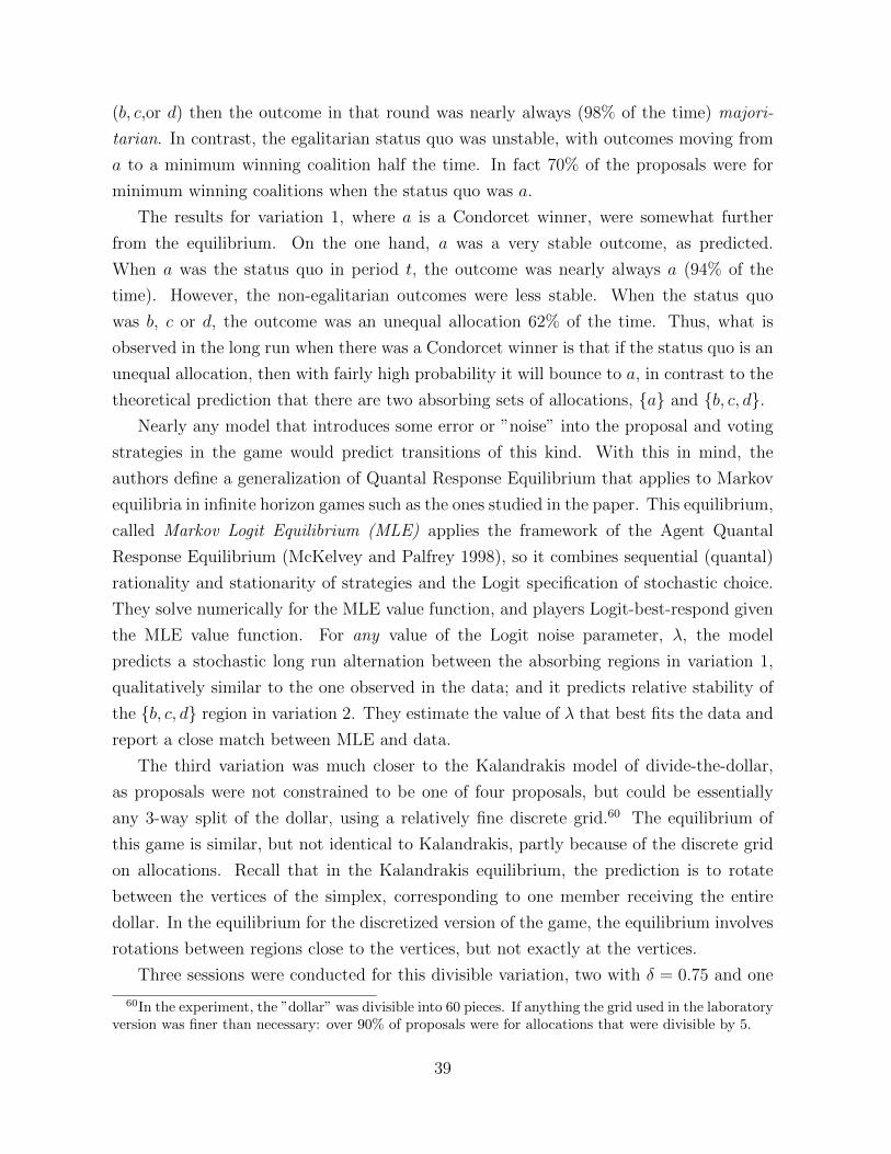
(b, c,or d) then the outcome in that round was nearly always (98% of the time) majori-

tarian. In contrast, the egalitarian status quo was unstable, with outcomes moving from

a to a minimum winning coalition half the time. In fact 70% of the proposals were for

minimum winning coalitions when the status quo was a.

The results for variation 1, where a is a Condorcet winner, were somewhat further

from the equilibrium. On the one hand, a was a very stable outcome, as predicted.

When a was the status quo in period t, the outcome was nearly always a (94% of the

time). However, the non-egalitarian outcomes were less stable. When the status quo

was b, c or d, the outcome was an unequal allocation 62% of the time. Thus, what is

observed in the long run when there was a Condorcet winner is that if the status quo is an

unequal allocation, then with fairly high probability it will bounce to a, in contrast to the

theoretical prediction that there are two absorbing sets of allocations, {a} and {b, c, d}.Nearly any model that introduces some error or ”noise” into the proposal and voting

strategies in the game would predict transitions of this kind. With this in mind, the

authors define a generalization of Quantal Response Equilibrium that applies to Markov

equilibria in infinite horizon games such as the ones studied in the paper. This equilibrium,

called Markov Logit Equilibrium (MLE) applies the framework of the Agent Quantal

Response Equilibrium (McKelvey and Palfrey 1998), so it combines sequential (quantal)

rationality and stationarity of strategies and the Logit specification of stochastic choice.

They solve numerically for the MLE value function, and players Logit-best-respond given

the MLE value function. For any value of the Logit noise parameter, λ, the model

predicts a stochastic long run alternation between the absorbing regions in variation 1,

qualitatively similar to the one observed in the data; and it predicts relative stability of

the {b, c, d} region in variation 2. They estimate the value of λ that best fits the data and

report a close match between MLE and data.

The third variation was much closer to the Kalandrakis model of divide-the-dollar,

as proposals were not constrained to be one of four proposals, but could be essentially

any 3-way split of the dollar, using a relatively fine discrete grid.60 The equilibrium of

this game is similar, but not identical to Kalandrakis, partly because of the discrete grid

on allocations. Recall that in the Kalandrakis equilibrium, the prediction is to rotate

between the vertices of the simplex, corresponding to one member receiving the entire

dollar. In the equilibrium for the discretized version of the game, the equilibrium involves

rotations between regions close to the vertices, but not exactly at the vertices.

Three sessions were conducted for this divisible variation, two with δ = 0.75 and one

60In the experiment, the ”dollar” was divisible into 60 pieces. If anything the grid used in the laboratoryversion was finer than necessary: over 90% of proposals were for allocations that were divisible by 5.

39

with δ = 0.83. In both cases, there was a lot of clustering and stability to allocations

far away from the vertices, in contrast to the theory. In fact, outcomes close to the

vertices were quite rare (less than 20% of the time). Outcomes were either perfectly or

nearly egalitarian more often than that, and over 60% of the allocations were approxi-

mately minimum winning coalition allocations where two of the members received large

allocations, and the third member received a zero or token allocation. Using numerical

computations to characterize neutral solutions when utilities are concave rather than lin-

ear, the authors are able to show that as concavity increases the long run distribution of

allocations becomes more equitable. Figure 6 shows the expected long run distribution

of allocations when voters have CRRA utility functions with parameter γ, where linear

utility corresponds to γ = 0.

Figure 6 about here.

Caption: Figure 6. Long run distribution of allocation for low (top panel) and high (bottom panel) levels of concavity.

In this sense the data suggest that perhaps the linear utility assumption is too strong.

Using MLE as an error structure the authors estimate the degree of concavity assuming

constant relative risk aversion. Their risk aversion estimate (approximately a square root

utility function) is close to what has been found across a broad range of other experimental

studies. Concavity is also consistent with the finding in variation 1, that the egalitarian

regime is much more stable than the regime corresponding to rotation between unequal

allocations. One final note about the behavior in these experiments is that behavior is

largely consistent with a model of perfectly selfish players, with little indication of other-

regarding preferences. Voting behavior in particular can be explained quite well by a

model of pure self interest.

Principal findings for dynamic divide-the-dollar games

1. Allocations over time are ”smoother” than predicted by the theory. This is consis-

tent with voters having concave utility functions.

2. Minimum winning coalitions are observed about as much as in BF bargaining games.

3. Proposals are usually accepted. Egalitarian proposals are fairly common and are

virtually always accepted.

Dynamic Legislative Bargaining with durable public goods Battaglini et al.

(2012) proposes a framework for studying the political economy of durable public good

40

production along the lines of models of economic growth. They establish some basic

theoretical results about the effect of the voting rule on the investment path of the public

good when the path is chosen over a sequence of periods with a legislative bargaining

game. Specifically, the environment consists of many citizens divided into n equally sized

districts, each with a single representative in the legislature. All citizens have the same

per-period utility function which is linear in the private good with an additively separable

concave utility, u(yt), for the current stock, yt of the durable public good. There is an

infinite horizon and a discount factor δ. In each period, there is an endowment equal to W

and a policy in period t is an n+1 vector, where the first component equals the investment

in the durable public good, It, and the last n components, xt = (x1t, ..., xnt) are the private

good transfers to each district. The investment increases the stock of the durable public

good, and the durable public good depreciates at rate d in each period. Hence, the stock

of public good in period t is equal to yt = (1− d)yt−1 + It, and an allocation sequence is

{xt, yt}∞t=1. Feasibility requires xt ≥ 0, yt ≥ 0, and yt +∑n

i=1 xit = W , for all t. Voter i

values an allocation sequence as the discounted sum of per-period utility of the sequence,

i.e.,∑∞

t=1 δt−1 [xit + u(yt)].

The bargaining game is simple. In each period one of the n legislators is randomly

selected to make a proposed allocation (yt, xt) and an up-down vote is conducted in the

legislature under a closed rule. Voting follows a q-rule where the proposal passes if

and only if it receives at least q votes in favor. If it fails, then a status quo outcome

occurs. They consider a simple exogenous status quo outcome, (y0, x0) where y0 = 0 and

xit = W/n for all i.

There are several theoretical properties of the model that can be examined by a lab-

oratory experiment. First, for all values of q and other parameters in the model, the

symmetric continuous Markov perfect equilibrium investment paths are inefficient. Sec-

ond, this inefficiency decreases with q.61 In the case of unanimity rule, the steady state

level of the stock of public good is actually equal to the optimal level, although the speed

of approach to the steady state is too slow, as proposers skim off some resources for private

consumption in each period.

The article reports results from an experiment with legislatures of size n = 5 and

three different voting rules: simple majority rule (q = 3), unanimity rule (q = 5), and

dictatorship (q = 1). In all the treatments, there is zero depreciation (d = 0), square root

61The Markov perfect equilibrium pins down predictions in these games. The entire set of subgameperfect equilibria is of course much larger, following folk theorem types of arguments. In fact, the efficientpath can even be supported in a subgame perfect equilibrium for large enough discount factors, includingthe parameters used in the experiments. The formal argument is in Battaglini et al. (2011a).

41

utility functions, and a discount factor of 0.75 is implemented using a random stopping

rule with constant probability of 1/4. Figure 7 shows the median time paths of yt for the

first 10 periods, for each of the three q rules. The theoretical equilibrium levels of yt are

marked in the figure.

FIGURE 7 ABOUT HERE

Caption: Figure 7: Comparison of theoretical and median observed time paths of yt for different voting rules.

There are several main findings. First, consistent with the Markov perfect equilibrium, the

level of investment is far below the efficient level, and converges over time to levels much

closer to the steady state of the Markov perfect equilibrium.62 Second, the unanimity

voting rule produces the most efficient outcomes, dictatorship the least efficient, and

majority rule in between, as predicted. Investment with q = 3 (majority) levels off at

nearly triple the size compared to q = 1 (dictatorship). Investment with q = 5 (unanimity)

converges to approximately six times the size compared to q = 1.Third, the path of

convergence to a steady state is different from the theory. There is overshooting. That is,

the legislatures overinvest in early rounds and then disinvest in later rounds. In all three

q treatments, the trajectory has the same pattern of early over-investment followed by

later disinvestment. Fourth, most proposals pass, as is consistent with the findings in the

static games discussed earlier. Fifth, approximately minimum winning coalitions are the

norm. While the proposals observed often have positive transfers to all districts, most of

the transfers are concentrated in a minimum winning coalition.

Battaglini et al. (2014a,2014b) consider a variation of the model in which the invest-

ment in the stock of public good in each period is made in a completely decentralized way,

with each district deciding independently how much of their (equal) share of the endow-

ment (W/n) to invest in the public good. This produces an economic environment that

is a dynamic voluntary contribution game, where the public good is durable rather than

the standard static model where the public good is nondurable. The voluntary contri-

butions mechanism is similar to many of the more traditional static public goods games,

as surveyed in Ledyard (1995). The main difference is that with a durable public good,

the public good level increases over time, and current contributions add to the stock of

the public good, which produces a stream of public benefits over time. In the traditional

static public goods experiments, public good contributions only produce benefits in the

current period. Often those traditional public goods experiments are repeated several

times in order to study learning dynamics, but there is no accumulation of stock; the

62The efficient level of investment required investing 100% of the endowment in all of the first 10periods.

42

level of public good is zeroed out at the start of each period.

The durable public goods experiment with decentralized public good investments is

reported in Battaglini et al. (2014b), and the design is organized in a way to examine the

theoretical results reported in Battaglini et al. (2014a). The latter paper characterizes

the symmetric continuous Markov perfect equilibria of the game and obtains comparative

static results with respect to the discount factor, the rate of depreciation, the group size,

and the concavity of the utility function. It also considers two different technologies

of public good production, depending on whether investments in the public good are

reversible. In particular they show that the reversible case leads to lower public good

contribution than the irreversible case. This comparison is especially stark in the case of

no depreciation, so the experiments focus on that case.

The experiment reported in Battaglini et al. (2014b) varies the group size between 3

and 5 and includes both reversible and irreversible investment treatments. The discount

factor of δ = 0.75 is used in all treatments. The basic procedures are similar to the leg-

islative bargaining, with the only difference being the voluntary contribution mechanism

instead of the legislative bargaining mechanism.The two main findings are that (a) there

are significantly more contributions with irreversible investments than in the reversible

case; and (2) there are also more contributions with n=5 than with n=3, but the differ-

ence is small and not significant. Figure 8 shows the median time paths of yt for the first

10 periods. The theoretical equilibrium levels of yt are marked in the figures.

FIGURE 8 ABOUT HERE

Caption: Figure 8: Comparison of theoretical and median observed time paths of yt in dynamic free riding experiment.

The experiment generally finds support for the predictions of the Markov perfect equi-

librium, but with similar caveats as described above with respect to the Battaglini et al.

(2012) experiment.

Principal findings for durable public goods experiments

1. Most proposals are for (approximately) minimum winning coalitions and most pro-

posals pass.

2. The proposer has significant proposer power.

3. Efficiency is increasing in the q rule, as predicted by the Markov perfect equilibrium,

and much less than the optimal solution.

43

4. The public good level converges to approximately the long run steady state of the

Markov perfect equilibrium.

5. The dynamics of convergence is characterized by overshooting the steady state in

early periods, and then either leveling out (if investments are irreversible) or drifting

back down through disinvestment toward the equilibrium steady state.

6. Voting behavior is generally consistent with long run optimal behavior, in the sense

of the Markov perfect equilibrium value function.

7. Contributions are higher when investments in the public good are irreversible.

3 Elections and Candidate Competition

While the first wave of experiments in positive political economy centered around coop-

erative game theory and unstructured bargaining in committees under majority rule, a

second wave of political science experiments followed quickly on the heels of the first, and

investigated the question of Condorcet winners and the majority rule core in the context

of competitive elections rather than small committees. These studies address many of the

same questions that have received the attention of empirical political scientists. The key

questions we will focus on here are: (1) spatial convergence of candidate platforms in com-

petitive elections; (2) retrospective voting; and (3) the importance of polls in transmitting

information to voters and coordinating voting behavior in multi-candidate elections.

3.1 The Spatial Model of Competitive Elections and the Median

Voter Theorem

3.1.1 Two candidate elections with a majority rule core

The median voter theorem says that under certain conditions, in two-candidate winner-

take-all elections, candidate platforms will converge to the ideal point of the median voter.

The theorem applies under fairly general conditions in one-dimensional policy spaces with

single-peaked preferences, and under more stringent conditions in multidimensional pol-

icy spaces. Basically, if Condorcet winners exist, they correspond to the symmetric pure

strategy Nash equilibrium of the game between two office-motivated candidates. Casual

observation indicates significant divergence of candidate and party platforms, even in

winner take all elections. Laboratory experiments can help us understand why this may

44

happen by providing some empirical evidence about the conditions required for conver-

gence.

There has been extensive work on candidate competition where voters have Euclidean

preferences and a Condorcet winner exists. The early contributions to this effort are

mostly by McKelvey and Ordeshook, and much of this is detailed in their 1990 survey.

The focus of this work has been on questions about the informational conditions that

are needed for convergence to equilibrium in candidate competition games. The simplest

and least challenging environment is one where the candidates have complete information

about voter preferences, so the existence and location of the Condorcet winning platform

is common knowledge.63 This is the environment used in their initial study (McKelvey

and Ordeshook 1982), which was further simplified by having only candidates as subjects,

with the behavior of five voters implemented by automatically voting for the closest

candidate. There were 10 repetitions of the candidate competition game. In each play

of the game the candidates simultaneously chose locations in a two-dimensional space,

and were then told the electoral outcome and the location chosen by the other candidate.

A candidate received a positive payoff whenever they won an election, with ties broken

randomly if they chose the same location. Outcomes converged to the Condorcet point.64

The distribution of outcomes in the last five repetitions is shown in Figure 9. More than

half of the observations are exactly at the majority rule core point.

FIGURE 9 ABOUT HERE

Caption: Figure 9. Election outcomes in last 5 repetitions. xi denotes the ideal point of voter i.

More challenging environments involve relaxing the assumption that candidates have

complete information and implementing voting behavior with human subjects rather than

by artificial actors.

Principal finding for competitive elections with a core

• When a majority rule core point exists, with enough repetition and learning, the

outcomes of an election game between two candidates converges to the Condorcet

winner. If a majority rule core point fails to exist, outcomes are concentrated in a

63There were five voters in a two-dimensional space, with Euclidean preferences. Voter ideal pointswere the same as in some of their committee experiments.

64McKelvey and Ordeshook (1982) also includes results from a series of elections with similar proce-dures, but where a Condorcet winner did not exist. In this case, there is no pure strategy equilibrium.They find that the candidate locations converge to a central area in the Pareto set, and conjecture thatbehavior is close to the mixed strategy equilibrium of the game.

45

central region of the Pareto set, as if generated by the distribution of locations in a

mixed strategy equilibrium.

3.1.2 Information aggregation by pre-election polling

The first experiment where polls are used to aggregate information were conducted by

Plott in the mid-1970s, with the results later published in Plott (1991). In these experi-

ments, there were between 19 and 41 voters (human subjects) with ideal points in a two

dimensional space, configured so that there was a Condorcet winning point. There were

two office-motivated candidates65 who were uninformed of the voters’ ideal points. All

they knew was that the policy space was a specific rectangle in two-dimensional space. In

each election, candidate positions were initialized near the edge of the policy space, far

from the Condorcet winner. At any time, either candidate could revise their platforms

by announcing a new (tentative) location. Candidates could also query voters about how

many would prefer them to move in some direction. In addition, public straw votes were

conducted periodically by the experimenter, based on the current (tentative) platforms of

the two candidates. At the end of a pre-specified time period, each candidate announced

his or her final position, which could not be changed. The election was then held, with

the winner receiving $10 and the loser $1. The data include 10 such elections with two

candidates. In 7 of 10 elections, the outcome was exactly the Condorcet point. The other

three elections resulted in outcomes very close to the Condorcet point.

McKelvey and Ordeshook (1985a, 1985b) push the information question further, by

studying elections where voters have poor information about the candidate locations. In

these studies, they pursue a variety of issues, mostly related to the question of how much

information was required of voters and candidates in order for competitive elections to

converge to the Condorcet winner. Perhaps the most striking experiment was reported in

McKelvey and Ordeshook (1985b) study of candidate competition in a one-dimensional

policy space. In this experiment not only did candidates have no information at all

about voters, but only half of the voters in the experiment knew where the candidates

were located. The rest of the voters were only informed about the left-right ordering of

the candidates. The key information transmission devices they explored were polls and

interest group endorsements. In a theoretical model of information aggregation adapted

from the rational expectations theory of markets, they proved that this information alone

is sufficient to reveal enough to voters that even the uninformed voters behave optimally,

65There were also some three candidate elections, which are discussed later in this survey.

46

i.e., as if they were fully informed.66 A corollary of this is that the candidates would

converge to the location of the median voter. Two sessions were conducted, each with

two candidates and between 40 and 50 voters. The game was repeated eight times to

allow for learning and convergence. The experiment finds strong support for candidate

convergence as if information were fully revealed to voters, and even more surprisingly,

they converge very close to the median voter. Figure 10 shows the time path of locations

of the candidates for each of the two sessions, with MT denoting the ideal point of the

median voter, MI denoting the ideal point of the median informed voter, and MU denoting

the ideal point of the median uninformed voter.

Figure 10 here, from p. 84 of JET paper

However, in an extension of this experiment to two dimensions, candidate convergence is

much slower; only half the candidates converge to the Condorcet winner with replication.

A number of studies have followed up on this theme of limited information elections.

Dasgupta and Williams (2002) also explore the information transmission properties of

polls when some voters are informed and others are not. Their setup differs in a number

of ways. First, candidates differ along a quality, or valence, dimension as well as a policy

dimension. The policy positions of the candidates are assigned by the computer and

publicly known. One is assigned the left-most position on a one-dimensional scale, and

the other is assigned the right-most position. Second, the quality type of each candidate is

unknown to voters at the time of election, but a subset of voters receive some information

about the quality of one of the candidates, who has an opportunity to take a costly action

to increase voter beliefs about his quality.67 A sequence of three opinion polls (straw votes)

is then conducted with all voters participating in the poll, with the outcomes publicly

observed. Then the actual election occurs and payoffs accrue based on the outcome. In a

manner similar to McKelvey and Ordeshook (1985b), they develop a rational expectations

equilibrium model adapted to this environment, in which information of the informed

voters is transmitted to the other voters as a result of the polls. The findings are broadly

supportive of the information aggregation properties of polls.68

66Voters also are assumed to know approximately where they stand relative to rest of the electorate ona left right scale.

67This is done by having the active candidate investing in effort, before knowing his own quality level.This produces a signal equal to the sum of the effort choice and his realized quality level. The signal isthen revealed to a subset of the voters. The motivation behind this signal structure is that the activecandidate is an incumbent coming up for re-election and the signal is some measure of his performancein office during his first term.

68In a related study, Lupia (1994) investigates a different mechanism for information revelation in direct

47

Principal findings for information aggregation by pre-election polling

1. Poll information and interest group endorsements successfully aggregate information

even when most voters have very little information a priori.

2. This kind of public information is sufficient to lead to convergence of candidates to

the majority rule core point with sufficient repetition.

3. The convergence to the core point is much slower in two dimensional policy spaces.

4. The information aggregation properties of polls extends to aggregating information

about candidate quality.

3.1.3 Retrospective voting

Political scientists have often wondered whether competitive electoral outcomes can arise

purely from retrospective voting. The earlier set of experiments with rational expecta-

tions and polls was entirely forward-looking and evaluation of candidates was prospective,

very much in the Downsian view of electoral competition. But many leading figures in

political science have argued that voter evaluations of candidates are backward-looking

and individual voting decisions depend largely on past records of candidates or current

economic conditions.69 Collier et al. (1987) and McKelvey and Ordeshook (1990)70, study

two-candidate elections where voters observe only the payoff they receive from the win-

ning candidate – not even the policy adopted by the winning candidate, nor the proposed

policy (or payoff) of the losing candidate. There are no campaigns or polls. Voters either

re-elect the incumbent or vote him/her out of office, in which case the other candidate

becomes the new incumbent. ”Voters observe historical information about their payoffs

(real income) derived from the policies (spatial positions) of previous incumbents, but

they do not observe these policies directly. Further, to model the situation in which vot-

ers do not even conceptualize elections in terms of issues, the voters in our experiments

are uninformed about the specific relationship (payoff function) between an incumbent’s

policy and their welfare. Nor do they know that an incumbent’s strategy concerns the

selection of positions in some policy space.” (McKelvey and Ordeshook 1990, p. 283)

legislation elections. His experiment demonstrates that when incompletely informed voters have informa-tion about the incentives of the author of ballot initiatives, they can use this information to increase thelikelihood they cast the same votes they would have cast had they possessed perfect information aboutinitiative.

69See Key (1966) and Fiorina (1981).70The latter article also summarizes results from the experiments on contemporaneous information

such as poll results or endorsements.

48

Candidates are somewhat better informed, in that they know what the policy space is,

and they observe all the platforms that their opponent has adopted in the past when in

office, as well as the past election results. However, candidates are given no information

about the distribution of voter ideal points nor how each voter has voted in past elec-

tions. The main finding is that on average candidates converge to the median, even in

this information-poor environment (McKelvey and Ordeshook 1990b).

In the baseline treatments, candidates receive a dollar each period they are the incum-

bent. Approximate convergence of candidate platforms is not immediate but generally is

achieved by the end of the session, after many repetitions. Figure 11 illustrates platform

convergence for three different session lasting between 30 and 45 periods.

Figure 11a here. Figure 11b here Figure 11c here from Collier et al pp. 106-107 (figs 1,2,4)

This figure should be arranged as three horizontal panels, and the whole thing called ”figure 11”.

In the figures, the median voter’s ideal point is marked by the dashed line, and the points

connected by the solid line represent the winning platforms in each round (which voters of

course do not see). Platforms converged almost perfectly to the median voter’s ideal point

in the session illustrated in the left panel of the figure, after a brief period of volatility

at the beginning when candidates were still learning. There were several variations on

this baseline design to explore the robustness of this convergence. In the first extension,

candidates have policy preferences. Rather than earning a fixed amount when elected,

the incumbent receives a payoff that is a linearly increasing function of the location they

choose in the [0, 100] interval. Convergence is still achieved, although more slowly. In

the next variation, the two candidates have opposing policy preferences, one candidate’s

payoff function is linearly increasing on the [0, 100] interval, but the other’s is linearly

decreasing. Again, convergence is achieved, but with a clear alternation of policies. See

the middle panel of figure 11. Finally, they conducted a variation where the location of

the median voter was shifted after period 21, without informing the candidates of this

shift. Although there is a slight lag, candidates converge surprisingly fast to the new

median location. See the right panel of figure 11.

One of the collective implications of these results about elections with limited infor-

mation is that it appears to be irrational for voters to gather costly information, if other

sources of information such as polls, endorsements, incumbent past performance, and

word-of-mouth are virtually free. This point is made explicitly in Collier et al. (1989)

which explores the question with 24 laboratory elections where voters are given an oppor-

49

tunity to purchase information about challenger’s policy if elected, in addition to the free

retrospective information that all voters receive about the past performance of the incum-

bent. That paper and Williams (1991) explore voter behavior and candidate convergence

by giving voters the option to gather costly information about candidates. They find that

the amount of information purchased by voters is correlated in the expected (negative)

way with the stability of candidate strategies, the imprecision of the information, and the

probability of casting a pivotal vote.

While this research does not resolve long standing questions about the responsiveness

of democratic institutions, it does add to what we understand about responsiveness by

demonstrating conditions under which incompletely informed voters can generate the

electoral outcomes that they would have if better informed. This research also informs

the debate about the use of the referendum and initiative to determine policy. One answer

to the question, ”Is direct legislation a useful mechanism for obtaining policy outcomes

that correspond to the will of the majority or is it a way for small, wealthy interest groups

to subvert the popular will?” is that direct legislation can be both. When voters are poorly

informed (or the electoral alternatives are reasonably complex), and there are no effective

information cues available, small groups who have enough resources to obtain agenda

control can use direct legislation to obtain preferred outcomes. When meaningful cues

are available (or the effect of electoral alternatives are easy to understand), then direct

legislation can be a useful tool for the implementation of majority-preferred policies.

These experiments establish two important facts. First, even in laboratory elections

where the stakes are low, election outcomes are well-approximated by median voter theory.

The Condorcet winner (core) is an excellent predictor of competitive election outcomes.

Second, this result is robust with respect to the information voters have about candidates

and the information candidates have about voters. Precious little information is needed

– a result that mirrors laboratory demonstrations that markets converge quickly to com-

petitive equilibrium prices and quantities, even with poor information and few traders.

In the discipline of political science, there has been great concern about how uninformed

most of the electorate is about candidates and policy issues. One reason for this con-

cern was a widely shared belief that these information failures could doom competitive

democratic processes. The McKelvey and Ordeshook series of experiments casts doubt

on this doomsday view. Just as financial markets can operate efficiently with relatively

few uninformed traders, or with many slightly informed traders, the forces of competition

can lead to election outcomes that accurately reflect public opinion, even if voters know

50

very little about the candidates and vice versa.71

Principal findings for information aggregation by retrospective voting

1. Historical information about past performance of candidates is sufficient to lead to

convergence of candidates to the majority rule core point with sufficient repetition

in simple environments.

2. The findings are robust with respect to a variety of modifications of the environment,

including unannounced shifts of the median voter location and extreme candidate

policy preferences.

3. All the findings of this section are broadly supportive of the hypothesis that com-

petitive elections can lead to Condorcet outcomes even when voters have very poor

information, in sufficiently simple environments.

3.2 Multi-candidate elections

In many elections, more than two candidates are competing for a single position using

plurality rule. In these multi-candidate elections, there is a natural ambiguity facing

voters in the form of a coordination game, and equilibrium places few restrictions on

outcomes: i.e., there are multiple Nash equilibria. To illustrate this, consider a three-

candidate election, with the candidates, A,B, and C having three distinct positions on a

one-dimensional issue scale, say the interval [−1, 1]. Suppose there is a large number of

voters with ideal points scattered along the interval. Voters know their own ideal point,

but have only probabilistic information about the other voters. Then, in a winner-take-all

election, for any pair of candidates, {i, j} there is a Bayesian equilibrium in which only

these two candidates receive any votes, with each voter voting for whichever of the two is

closer to their ideal point. This is an equilibrium because it never (instrumentally) pays

to vote for a candidate who nobody else is voting for. Indeed there can be some other

equilibria, too (Palfrey 1989, Myerson and Weber 1995), but 2-candidate equilibria are

the only ones that are stable (Fey 2000). Voters face a coordination problem. Which

two candidates are going to be receiving votes? Will a Condorcet winner be chosen if it

exists?

71Of course, these experiments explore relatively simple environments and focus only on the maindriving force of candidate competition. Future research will need to address the role of other factorssuch as voter turnout, campaign contributions, advertising, the role of parties and primaries, valencedimensions, and so forth.

51

Forsythe et al. (1993, 1996) explore these and other questions in a series of exper-

iments. Their laboratory elections had three categories of voters defined by different

preference orders over the three candidates. One group preferred A to B to C. The sec-

ond group preferred B to A to C, and the third group ranked C first and was indifferent

between A and B. The third group was the largest, but was less than half the popula-

tion. Groups one and two were the same size. The actual payoff tables and preference

configurations are given in Table 1.

Preference type Winner #Voters

A B C

1 $1.20 $0.90 $0.20 4

2 $0.90 $1.20 $0.20 4

3 $0.40 $0.40 $1.40 6

Table 1. Voter preferences in Forsythe et al. (1993,1996).

Hence, if voters voted for their first choice, C will win, but C is a Condorcet loser, since

it is defeated by both A and B in pairwise votes. There are several equilibria, including

the two where type 1 and 2 voters coordinate on either A or B. However, because of the

special configuration of preferences and because there is complete information, sincere

voting is also an equilibrium, resulting in the Condorcet loser, C, winning.

The procedures were carefully designed to avoid repeated game effects, to minimize

possible effects of extraneous coordination devices, and at the same time allow subjects to

gain experience at the task.72 Each experimental session was conducted with 28 subjects

divided into 14-member voting groups, and repeated over a series of 24 periods. Thus

each session generated data for 48 elections, with 14 voters in each election. Voting groups

and preference types were randomly reshuffled after every election.73

First, the authors note that without any coordinating device, there is coordination

failure. Some voters in groups one and two vote strategically (i.e., for their second choice,

trying to avoid C) but many don’t, and the strategic behavior is poorly coordinated, so

as a result the Condorcet loser wins 90% of the elections.

Second, they look at three kinds of coordinating devices: polls, past elections, and

ballot position. Polls allow the voters in groups 1 and 2 to coordinate their votes behind

either candidate A or candidate B. This is indeed what usually happens. The Condorcet

72For example the alternatives were labeled Orange (A), Green (B), and Blue (C) to avoid alphabeticalorder as a coordinating device.

73An exception is Forsythe et al. (1996), where voting groups were reassigned only after every eightelections.

52

loser wins only 33 percent of the elections. Moreover, when either A or B is first ranked in

the poll, the Condorcet loser wins only 16 percent of the time. Election history also helped

with coordination. There was a small bandwagon effect between A and B. Whichever was

winning in past elections tended to win in future polls. Ballot position had an effect on

voting strategies, but the effect was too small to influence election outcomes.

Their second paper looks at alternative voting procedures, comparing plurality rule

to the Borda Count (BC) and Approval Voting (AV). 74 Both procedures worked better

than plurality rule, in the sense that the Condorcet loser was more easily defeated. Both

procedures tended to result in relatively close three-way races with A or B usually winning.

Plurality, in contrast, produced close three-way races, but with C usually winning. A later

study by Bassi (2008) delves more deeply into a comparison of strategic behavior under

these three voting rule. That study differs from the earlier studies in three ways: the

preference profile, the number of voters (5 instead of 14), and the number of alternatives

(4 instead of 3). The two profiles employed in the design have the property that iterated

deletion of dominated strategies eliminates all but one equilibrium, so the coordination

problem created by multiple equilibria is not present. The main finding is that voting

is most sophisticated (i.e., most consistent with equilibrium) under plurality and least

sophisticated under BC, with AV in between.

Rietz et al. (1998) follow up this experiment with a very similar one that explored

whether campaign contributions can have a similar coordination effect. In this variation,

before each election, each voter independently decided on campaign contributions. Each

voter was allowed to contribute (at real expense) up to $0.20 in penny increments. These

contributions could be spread across any subset of candidates, or none at all. The total

contributions for each candidate were then publicly revealed prior to the election stage.

The results were similar to the results from the polling treatment, with the Condorcet

loser winning only 33% of the time. The type 1 and 2 voters generally coordinated on

whichever candidate, A or B, received the most contributions. Moreover, even accounting

for its direct cost, campaign contributions increased coordination enough to lead to higher

overall efficiency compared with no contributions.

Another question is whether campaign contribution decisions were consistent with an

equilibrium of the two stage game. The paper does not offer any model of equilibrium

for the more complicated game, where the first stage is contribution and the second

stage is voting, but instead argues that the contribution levels do not seem irrational, at

74The BC rule requires voters to rank the candidates from most preferred to least preferred. Thecandidate with the highest average ranking wins. AV is similar to the plurality voting rule, except votersare permitted to vote for more than one candidate. The candidate with the most votes wins.

53

least for the type 1 and 2 voters, in the sense that the marginal benefit from an additional

incremental contribution is lower on average than the cost, while the marginal benefit from

the last nickel contributed is higher.75 However, this is done as a back-of-the-envelope

calculation rather than a careful statistical analysis, and there is a significant free rider

dimension in the contribution stage.

There are a number of other papers that conduct experiments on related three-

candidate coordination games. The earliest work is by Plott (1991)76, who investigates

3-candidate races in a two-dimensional policy space. The setting is different in the sense

that candidate locations were endogenous, and were sequentially chosen, and mixed in

with occasional straw votes, with the same procedures as described for the 2-candidate

elections reported in the same paper. Thus, candidates were adjusting positions over time,

and there was a majority rule core. Unfortunately, there is little guidance in the way of

useful predictions based on Nash equilibria. Still, winning candidate locations tended to

converge to the core, but with only slightly more more variance than in the 2-candidate

baseline treatment. In the ten 3-candidate elections, three outcomes were exactly at the

Condorcet point and the seven others were close. See Figure 12.

Figure 12 about here.

Caption Winning platforms in three candidate elections. Plott (1991 p. 22)

Felsenthal et al. (1988) and Rapoport et al (1991) examine bloc voting in three can-

didate elections, where all voters with identical preferences vote identically. Their design

considers a variety of preference profiles in order to compare the predictions of several al-

ternative voting models for selecting among the many Nash equilibria of the game. They

propose a model of equilibrium selection based on implicit cooperation between voting

blocs with similar but not identical preferences. For several of the preference profiles they

study, coordination is consistent with their model a large fraction of the time.

Gerber et al. (1996) and Morton and Rietz (2008) explore the multi-candidate coor-

dination problem with different electoral institutions. Gerber et al. look at cumulative

voting when two rather than one candidate is to be elected, to see if it can ameliorate

problems of minority under-representation due to mis-coordination. Voters are endowed

with two votes. In the baseline treatment they can cast one vote for each of two differ-

ent candidates, only one vote for one candidate, or no votes for any candidate. In the

75On the other hand, it seems harder to rationalize the contribution decisions of the type 3 voters.76The results were obtained much earlier than the publication date, and presented at the 1977 Public

Choice conference.

54

cumulative voting treatment, they have an additional option to cast two votes for one

candidate. The top two vote getters are elected. They use the same preference profile as

in Forsythe et al., and payoffs are additive with respect to the two winners of an election.

In the baseline treatment, the theoretical prediction is that C will never win, but C should

win under cumulative voting. The data closely matches the theory. Morton and Rietz

consider runoff elections where winning requires a clear majority. If there is no majority

winning in the first round, then the two top candidates engage in a runoff election in the

second round. This also helps solve the coordination problem in a similar way to polls:

whichever of the two minority candidates is in the runoff wins.

To summarize, multi-candidate elections are an intriguing and immensely complex

brand of coordination problem. Outcomes are extremely sensitive to the fine details of

the voting institutions as well as the myriad of coordinating devices related to those insti-

tutions (polls, history, party labels, campaign contributions, and even cheap talk). This

would seem to be a rich area for both experimental and theoretical research. An obvious

direction to explore is to look at the endogenous entry of candidates and endogenous pol-

icy positions of candidates. All these experiments fix the number of competing candidates,

and even fix their policies (except for Plott 1991).

Principal findings for multi-candidate elections

1. In the absence of coordination devices, simple plurality rule can lead to poor out-

comes (Condorcet losers) in multi-candidate elections

2. Very simple coordination devices, such as polls, publicly revealed campaign contri-

butions, and past electoral outcomes, can help alleviate coordination problems.

3. If a Condorcet winner exists, competitive elections under plurality rule with three

candidates converges toward the core point, but with more variance than in two

candidate elections.

4. Voting rules other than plurality rule (Borda count, approval voting, runoff, etc.)

can outperform plurality rule in specific environments.

5. All of the above results are based on a very limited set of environments that have

been studied in the laboratory.

55

3.3 Candidate competition with valence

In many elections, candidates are asymmetric. A widely cited source of asymmetry is

incumbency. It is generally thought that incumbents have a significant advantage over

challengers, above and beyond any advantage (or disadvantage) they may have due to spa-

tial location. Other sources of asymmetries include valence characteristics of candidates,

such as a familiar name, movie or athletic star status, height, articulateness, and person-

ality traits. The two key aspects of these valence characteristics are: (1) most voters value

them, independent of the candidate platforms; and (2) they are fixed, rather than being

chosen by the candidates. With strategic competition, candidate asymmetries have inter-

esting and systematic implications for equilibrium platforms. These asymmetric contests

have been studied recently both theoretically and empirically in game theoretic models by

Erikson and Palfrey (2000), Ansolabehere and Snyder (1999), Groseclose (2002), Aragones

and Palfrey (2003, 2005), and others.

Groseclose (2002) and Aragones and Palfrey (2003, 2005) show that valence asymme-

tries lead to candidate divergence, even in one-dimensional spatial models. The equilibria,

which can be either mixed strategy equilibria or pure strategy equilibria (if candidates

have policy preferences and there is enough exogenous uncertainty) have two interesting

features. First, a disadvantaged candidate will tend to locate at more extreme locations

in the policy space than the advantaged candidate.77 Second, the extent to which this

happens depends on the distribution of voters, in a systematic way. As the distribution

of voter ideal points becomes more polarized (e.g., a bimodal distribution), the disadvan-

taged candidate moves toward the center, while the advantaged candidate moves in the

opposite direction, and adopts more extreme positions.

Aragones and Palfrey (2004) report the results of an experiment designed to test

whether these systematic effects can be measured in a simplified spatial competition

environment. Candidates simultaneously choose one of three locations, {L,C,R}. The

location of the median voter is unknown, but they both know the distribution. The

median is located at C with probability α, and located at either L or R with probability

(1 − α)/2. Candidate 1 is the advantaged candidate; he wins if the median voter is

indifferent (in policy space) between the two candidates, which happens if the candidates

locate in the same position, or if one chooses L and the other R. Their main treatment

77The intuition is twofold. All else equal, both candidates would like to locate near the center, becausethat’s where the median voter is. However, the disadvantaged candidate can only win by distancinghimself away from the advantaged candidate, which leads to an incentive to move away from the me-dian. Mixing occurs because the advantaged candidate can win by matching any pure strategy of thedisadvantaged candidate.

56

variable is the distribution of the median, α, which in different sessions takes on values

of either 1/5, 1/3, or 3/5. The equilibrium is characterized by a pair of probabilities of

locating at the central location, one for the advantaged candidate (p) and one for the

disadvantaged candidate (q). These equilibrium probabilities are ordered as follows.

0 < q3/5 < q1/3 < q1/5 <1

3< p3/5 < p1/3 < p1/5 < 1

The data perfectly reproduce this ordering of candidate locations, for all treatments,

and the results are quantitatively close to the mixed strategy equilibrium choice probabil-

ities. The result appears to be robust, and has been replicated successfully with different

subject pools and instruction protocols. There are also now a number of theoretical re-

sults when the policy space is continuous instead of discrete (Aragones and Palfrey 2003,

Hummel 2010), and a natural ”next experiment” in this area would be to run a similar

experiment but in an explicitly spatial environment.

Asymmetric contests have also been studied in economics experiments. Perhaps the

best known is the study of tournaments rewards, by Bull and Schotter (1990), and interest

in studying these asymmetric contests has resurfaced recently in studies that look at the

tournament structure of labor markets as a possible reason for gender wage differentials

and glass ceilings (Gneezy et al. 2003). It would be interesting to extend this tournament

approach to study campaign spending in political campaigns. The problem is also closely

related to all-pay auctions, which have received some recent attention by experimental

economists.

Principal findings for elections with a valence dimension

1. In two way races along one dimension, higher quality candidates tend to adopt more

moderate positions.

2. This effect diminishes with more polarized distributions of voters.

4 Voter Turnout

Fiorina (1978) dubbed it ”The paradox that ate rational choice theory.” A typical state-

ment of the paradox is the following. In mass elections, if a significant fraction of voters

were to turn out to vote, the probability any voter is pivotal is nearly zero. But if the

probability of being pivotal is zero, it is irrational to vote because the expected benefits

would then be outweighed by any tiny cost associated with voting. Hence the fact that

57

we see significant turnout in mass elections is inconsistent with rational choice theory.

Voters must be voting for some other reasons, and rational choice theory is not a useful

approach to understanding political participation.

Palfrey and Rosenthal (1983) take issue with the logic of the paradox. They point

out that turnout should be modeled as a ”participation game”, and that zero turnout

is not an equilibrium of the game, even with rather high voting costs. In fact, as the

number of eligible voters becomes large (even in the millions or hundreds of millions),

they prove the existence of Nash equilibria where two-party elections are expected to

be quite close and turnout is approximately twice the fraction of the electorate that

prefers the underdog. Thus, in tight races, where there is no clear favorite, equilibrium

turnout can be nearly 100%. These high turnout equilibria also have some other intuitive

properties; for example, supporters of the underdog (who face less of a free rider problem

within their group) turn out at a higher rate than the supporters of the favorite.

4.1 Instrumental voting experiments

Schram and Sonnemans (1996) describe results from an experiment designed to not only

test the Palfrey-Rosenthal theory of turnout, but also to compare turnout in Winner-take-

all (W) elections to turnout in Proportional Representation (PR). They studied 2-party

elections with 12, 14, or 28 voters in each election. Voters were equally split between the

two parties, except in the 14 voter treatment, where there were 6 voters for party A and 8

for party B. In the PR elections, the cost of voting was 70, and the payoff to all members

of party j was equal to 222 · vj where vj was party j’s vote share. In the W elections, the

cost of voting was 100 and all members of the winning party received 250, with ties broken

randomly. All of this was made common knowledge by presenting the subjects with a

common set of instructions.78 Each session ran one of these treatments repeatedly, with

feedback, over a sequence of 20 elections. It was not a symmetric experimental design,

with most sessions using W elections. There were also some secondary treatments, and

some additional variations explored in Schram and Sonnemans (1996b). The main findings

were:

(a) Turnout in the early (inexperienced) W elections started around 50%, and declined

to around 25% by the last election. The decline was steady, and it’s not clear whether it

would have declined even further with more experience.

(b) Turnout in the early (inexperienced) PR elections started around 30%, and declined

to around 20% in the last two elections. The decline was very gradual in these elections,

78The instructions used neutral terminology, rather than presenting the task as a voting decision.

58

and it’s not clear whether it would have declined even further with more experience.

(c) The effects of electorate size and party size are negligible.

Exactly how to interpret these results is a difficult question. The theoretical predic-

tions of Palfrey and Rosenthal (1983) for the W elections are somewhat ambiguous because

there are many equilibria, including pure strategy equilibria (except in the 14-voter case),

totally mixed strategy equilibria, and mixed-pure equilibria. In fact, the range of possible

equilibrium turnout rates in each of the W games conducted in the experiment includes

much of the entire [0, 1] interval. The decline of turnout may indicate that behavior is

equilibrating, and might eventually converge to the low turnout totally-mixed equilibrium

(between 2% and 5% in the W games), if the experiments could have lasted long enough.

But this is highly conjectural. The symmetric equilibrium of the PR game was slightly

higher, about 10%. Again, one might conjecture that voter behavior is converging on this

equilibrium, but that is also highly speculative, and can only be answered definitively

with more experienced subjects (longer sequences of elections), or perhaps an alternative

design.

The biggest puzzle in the data is why initial turnout rates in the PR elections were

so much lower than initial turnout rates in the W elections. A possible explanation is

coordination failure and multiple equilibria. While both voting rules can have multiple

equilibria, it is only the W elections for which equilibria exist with high turnout rates

(above 50%). One interpretation of these experiments is that the severe multiple equi-

librium problems identified by the theory present tremendous strategic ambiguity to the

subjects and render the early round data almost useless for evaluating the effect of voting

rules and electorate size on turnout.79

Levine and Palfrey (2007) take a different approach to addressing comparative statics

questions about the effect of electorate size, relative party size, and voting cost on turnout

in W elections. Their design follows Palfrey and Rosenthal (1985), which extended their

1983 game-theoretic analysis of turnout to allow for heterogeneity of voting costs and

asymmetric information. In that model, all voters in a party have the same benefit of

winning, but each voter has a privately known voting cost that is an independent draw

from a commonly known distribution of costs. The symmetric equilibrium of these games,

with equal sized parties, is characterized by a simple cutpoint decision rule, where voters

with costs less than a critical cost, c∗ vote and voters with costs greater than c∗ abstain.

79Despite the problems with multiple equilibria, the experiments provide an interesting source of datafor understanding coordination failure and the dynamics of behavior in coordination games. Below wealso discuss the QRE analysis of these games by Goeree and Holt (2005), which provides a possibleexplanation for the early round differences in W and PR turnout rates and the eventual decline andconvergence of the two turnout rates.

59

For many cost distributions, there is a unique equilibrium cutpoint, so the coordination

problem is completely eliminated. The analysis is extended easily to unequally sized

parties, with the cutpoints typically different for the two parties.

They conduct an experiment where electorate size can take on values of 3, 9, 27, and

51. Winning pays off 105, losing pays off 5, and a tie pays off 55.80 Neutral instructions

were used, with no mention of voting, winning, or losing. The voting cost was framed

as an opportunity cost, the equivalent of an abstention bonus. For each electorate size,

N , there are two party size treatments, called toss-up (T) and landslide (L). In the T

treatment, the larger party has N+12

members and the smaller party has N−12

members. In

the L treatment, the larger party has 2N3

members and the smaller party has N3

members.

This produces a 4× 2 design.81 In all elections, there is a unique Nash equilibrium. The

comparative statics of the equilibrium in the various treatments are simple and intuitive.

Turnout should be decreasing in N for both parties - the size effect. Turnout should

be higher for both parties in the T treatment than in the L treatment - the competition

effect. Turnout should be higher for the smaller party than the larger party - the underdog

effect, with the exception of N = 3, an unusual case where the larger party has higher

equilibrium turnout.

The aggregate results conclusively support the Nash equilibrium comparative statics.

Figure 13 below compares the observed (vertical axis) upset rates82, and close election

rates83 to the Nash equilibrium predictions (horizontal axis) for all the experimental treat-

ments. The observation/prediction pairs line up almost exactly on the 45% line. A simple

linear regression gives an intercept of 0.01, a slope of 1.03, with an R2 = .99.

F igure 13 here. (Fig 2 from APSR p. 150)

Nearly all of the predicted qualitative comparative statics results are observed. In fact,

all the theoretical predictions about the competition effect84 and the underdog effect were

found in the data. All but one size effect prediction was observed.85 The results are also

80We chose to not to break ties randomly because there were already several random variables in thedesign (the assignment of voting costs and the assignment to parties), and this was simpler. Instead, tiespaid the expected value of a random tie break.

81When N = 3, the toss-up and landslide treatments are the same.82The upset rate equals the probability the minority candidate wins.83The close election rate is the probability the election is either tied or one away from a tie. That is,

the probability a voter is pivotal.84The competition effect is also supported in a recent experiment by Grosser and Schram (2010). They

compare turnout in 12 voter elections where the larger party can consist of 6, 7, 8, or 9 voters.85The size effect is supported with the exception for the tossup races with 27 versus 51 voters, where

turnout was slightly more (less than half a percentage point) in the 51 voter case than the 27 voter case.

60

very close quantitatively to the equilibrium predictions, with one caveat. The turnout

probabilities are somewhat less responsive to the treatment parameters than equilibrium

theory predicts.

These attenuated treatment effects are shown to be consistent with the logit version of

regular quantal response equilibrium (QRE). QRE replaces the assumption of perfect best

response to noisy best response. In its most general formulation (McKelvey and Palfrey

1995, 1998) this is modeled by adding privately observed payoff disturbances associated

with each strategy of each player, and at QRE is defined as a Bayesian equilbrium of

a game in which the joint distribution of all these additive payoff disturbances is com-

mon knowledge. In all applications to date, it is assumed that the disturbances for each

individual are are i.i.d., which implies that response functions are simply smoothed out

best response functions, with the choice frequencies of strategies by each player monotone

in expected payoffs.86 A regular QRE is a fixed point of these smoothed out monotone

response functions, just as Nash equilibrium is a fixed point of best response correspon-

dences. A relatively tractable parametrization uses Logit response functions, where the

probability player i chooses strategy sij, pij is given by:

pij =eλUij(p)∑

sij∈SieλUij(p)

.

where λ ∈ [0,∞). Then p∗ is a Logit QRE (sometimes called a Logit equilibrium) of a

particular game, for a particular value of λ, if and only if, for all i, j:

p∗ij =eλUij(p

∗)∑sij∈Si

eλUij(p∗)

Thus, for any game, the Logit specification defines a family of quantal response equilibria

parameterized by λ. When λ = 0 players are completely payoff unresponsive and choose

all strategies with equal probability. Limit points, when λ → ∞, are Nash equilbria,

although not all Nash equilibria can be approached by a sequence of Logit QRE.87 For

this reason, Logit QRE provides a method of selecting among Nash equilibria. In fact, for

almost all games there is a unique selection from the Nash equilibrium, called the Logit

86The distribution of disturbances can be different from different individuals. See Rogers et al. (2010).With no restrictions on the distribution of disturbances, choice frequencies are not necessarily monotone,and in fact can be anything. This is a general property of additive random utility models. See Haile etal. (2008) and Goeree et al. (2005).

87The definition has been generalized to extensive form games (AQRE). Limit points of AQRE asλ→∞ are sequential equilibria.

61

solution of a game, defined as the unique limit point that is connected in the graph to

the λ = 0 equilibrium. In many games, the Logit equilibria imply definitive comparative

statics or directional biases from Nash equilibrium choice probabilities.

Voter turnout games provide a convenient illustration of how such biases can arise, even

though the payoff disturbances to the players that underly the Logit model are completely

unbiased. In particular, the Logit QRE of these games predicts higher turnout than the

Nash predictions for large electorates, and lower turnout in the N = 3 treatment. Levine

and Palfrey (2007) use their data to estimate one free parameter of a Logit QRE model, λ,

based on their entire dataset. Then, based on this estimate, they can extrapolate to what

turnout would be in mass elections with hundreds of millions of potential voters. Such

an exercise implies that, for plausible distributions of voting costs, equilibrium turnout

rates in the Logit QRE model are on the same order of magnitude as what we observe

in nation-wide elections in the U.S. Since 1970, turnout in the U.S. national elections as

a percentage of the voting age population has ranged from 49% to 55% in presidential

elections and 36% to 47% in midterm elections. If the voting costs were positive for all

eligible voters and uniformly distributed, and the value of being a dictator in the election

(i.e., the benefit of unilaterally changing the election outcome from your least preferred

candidate to your most preferred candidate) is, for the average voter, 100 times the cost

of voting, then QRE expected turnout - based on the Logit parameter estimate in the

paper - in large elections is approximately 48%.

Furthermore, the Logit specification of stochastic choice also turns out to fit the in-

dividual choice data remarkably well. The stochastic choice model specifies that the

probability a voter votes in a given treatment is a smooth and continuously decreasing

function of voting cost, and is anchored by the treatment-specific equilibrium cutpoint

(i.e., the point where a voter is indifferent between voting and abstaining given the other

voters’ turnout strategies). At such an indifference point, the stochastic choice model pre-

dicts that the voter is equally likely to vote or abstain. Figure 14 shows the turnout rates

as a function of normalized88 voting costs including all treatments pooled together. The

points in the figure indicate the observed turnout frequency for a particular treatment

and party at each normalized voting cost, with horizontal bars indicating the overall av-

erage turnout at 0.03 intervals. The solid decreasing curve is the Logit choice probability

88In order to pool all treatments together, the horizontal axis represents the normalized voting cost,i.e., the difference between the voting cost and the equilibrium indifference point (which varies acrosstreatments).

62

function at the QRE, for the estimated value of λ = 7.

Figure 14 here. (Fig 4 from APSR p. 152)

Goeree and Holt (2005) apply a QRE analysis of symmetric equilibria for a broad

range of symmetric complete information game theoretic models of participation. They

consider the class of games where N players each have a binary choice (participate or

not), and the expected payoff to a player for participating or not, are given by P (p,N)

and NP (p,N), respectively, if all N − 1 other players are participating with probability

p.89 Examples of such games include variations on threshold public goods games (van de

Kragt, et al. 1983, Palfrey and Rosenthal 1984, 1988, 1991a, 1991b,1994), the volunteer’s

dilemma (Murnighan et al. 1993, Diekmann 1985,1986, Franzen 1995), voter turnout

(Palfrey and Rosenthal 1983, 1985), congestion games, and strategic entry in markets

(Meyer et al. 1992, Camerer and Lovallo 1999, Fischbacher and Thoni 2001, Sundali et

al. 1995). Goeree and Holt’s analysis organizes a wide range of observed behavior in

experiments, including some that had been considered anomalous from the standpoint of

traditional Nash equilibrium theory.90

A particularly relevant result for the present survey is the application by Goeree and

Holt (2005) of the QRE approach to the Schram and Sonnemans voter turnout studies

described at the beginning of section 4.1. First, as in the Levine and Palfrey analysis

with respect to voter turnout games with private information, QRE turnout rates are

biased toward 50%, compared to the Nash equilibria. Goeree and Holt demonstrate this

is also true for complete information voting games, using the low turnout symmetric

equilibrium as the relevant benchmark. For relatively low levels of λ (e.g., high error

rates by inexperienced players), they show that turnout will be higher for W elections

than in PR elections, but for higher values of λ the differences are smaller and for some

parameter values completely disappears. Moveover, for both voting rules turnout rates

decline monotonically in λ. All three of these properties are mirrored in the Schram and

Sonnemans study, as noted above.

The approach of modeling turnout as a Bayesian game with privately known voting

costs has recently been extended to compare turnout in PR vs. W electoral systems

by Herrera et al. (2014) and Kartal (2013). Theoretically it is shown that equilibrium

turnout is generally higher in W if the election is competitive and higher in PR if the

89Their analysis can be extended to studying quasi-symmetric equilibria in asymmetric participationgames.

90Cason and Mui (2004) independently proposed QRE as an explanation to some results they observein participation games.

63

election is a landslide. The intuition is that turnout in W is highly responsive to expected

closeness, while turnout in PR is not. The experiments reported in those papers provide

qualified support for this. This provides yet another alternative explanation for the higher

turnouts in PR elections that were reported in Schram and Sonnemans (1996), although

costs were homogeneous and common knowledge in that experiment.91

4.2 The effects of beliefs, communication, and information on

turnout

Duffy and Tavits (2008) conduct an experiment based on the complete information Palfrey

and Rosenthal (1983) model that, in addition to observing turnout decisions by individual

voters, also elicits beliefs from individual voters about the probability of a close election,

using a proper scoring rule. The objective of the design is to have a more direct test of the

pivotal voter hypothesis, and allow one to sort out possible deviations from equilibrium

depending on whether they are due to incorrect beliefs about the probability of being

pivotal, or other sources that have been hypothesized such as expressive voting (discussed

below). The former can be measured by comparing the belief about being pivotal to the

empirical distribution of margin of victory; the latter can be measured by comparing a

voter’s actual turnout choice with the turnout choice that would be optimal given their

beliefs about being pivotal. Regarding the former, they find that voters’ reported beliefs

about the probability of a close election are generally higher than the actual frequencies

in the experiment, although the bias in beliefs declines significantly with experience.

Regarding the latter, they find that turnout rates are positively correlated with reported

beliefs about pivot probabilities, as one would expect. However, voters systematically

turn out much less frequently than they should given their beliefs. In fact, they also vote

less than what would be optimal if they actually held empirically accurate beliefs, or even

if they had the equilibrium beliefs.

There are a number of possible explanations for these apparently contradictory find-

ings. On the one hand, if subjects are risk neutral, then either they are clearly not

optimizing given their beliefs, or the belief elicitation procedure failed.92 An alternative

explanation is risk aversion, which would have (at least) two effects in their experiment.

91Theoretically, there is a parallel between QRE in complete information turnout games with homo-geneous costs and Bayesian equilibria of the turnout games with privately known costs, because theprivately known costs can be interpreted as additive payoff disturbances.

92Some recent papers have cast doubt on the reliability of elicited beliefs from subjects during thecourse of a decision or game theory experiment. See Palfrey and Wang (2010) and several of the papersthey cite.

64

First, risk aversion would bias reported beliefs upward in the direction of .5 under the

Brier scoring rule. Second, risk aversion would lead to reduced turnout, since voting re-

sults in a certain loss in exchange for an uncertain gain. In any case, the data clearly cast

some doubt on the notion that non-negligible turnout rates in mass elections are mainly

due to voters overestimating the probability of being pivotal.

Grosser and Schram (2010) also use the 1983 Palfrey-Rosenthal participation game

model as the basis for their study of the effect of pre-election polling on turnout. In their

design, laboratory electorates of size 12 are divided into two parties of relative sizes 9-3,

8-4, 7-5, 6-6, 5-7, 4-8, or 3-9. The main treatment variable is whether or not voters are

informed about the exact relative sizes of the parties (the ”polling” treatment) or only

told the probability distribution of these relative sizes.93 There was no additional private

information beyond a voter’s knowledge of his own party preference. Benefits and costs

were the same for all voters, and this was common knowledge. They find that many of

their results are well explained by the Logit QRE. The two main findings are (i) that

polling led to higher turnout on average, with the greatest effect being when voters were

informed the party split was 6-6; and (ii) that, with full information, turnout was higher

in more competitive elections. The second effect was not just due to higher turnout in

the 6-6 cases. However, the first effect is entirely driven by the 6-6 cases. This could be

due to multiple equilibria, as 100% turnout is a second symmetric Nash equilibrium in

the 6-6 elections.

In a second study of informational effects on turnout, Grosser and Schram (2006) study

the role of information about other voters’ turnout decisions.94 In particular, they are

interested in identifying whether knowledge of other voters’ turnout decision can affect a

voter’s turnout decision. This could have potentially important ramifications for election

policies such as early voting and news delays on exit polls and election day returns. They

do so in a similar complete information 6-6 voter turnout game, but half of the voters in

each party are ”early” voters, and the remaining late voters can observe some information

about the early voting before deciding whether or not to vote.95 There are three different

information treatments. In the baseline, late voters are given no information. In the

second treatment, late voters are told the turnout decision of exactly one of the early voters

but are not told which party that voter belonged to. In the third treatment late voters

93Voters were assigned to parties in the following way. First, three voters were assigned to each party.Then the remaining six voters were each assigned to one or the other party by independent coin tosses.

94There is a large and growing literature in political science that uses field experiments and naturalexperiments to study various informational effects on voter turnout. See for example Gerber and Green(2000) and Lassen (2005).

95Early voters can vote in the second stage if they abstain in the first stage.

65

are told the turnout decision of exactly one of the early voters and also told which party

that voter belonged to. In the last treatment, the early voters are told in advance whether

their vote would be observed by a member of the same party or a different party. Each

late voter is told about one early voter’s turnout decision. Cases are distinguished where

the voters are allies (support the same group) or adversaries (with opposing preferences)

and where they are uncertain about each other’s preferences. From the quasi-symmetric

equilibrium Grosser and Schram solve for, two key hypotheses emerge. First, information

of this kind is predicted to increase overall turnout. Second, turnout rates for early voters

are higher than for late voters, largely because early voters may vote in either stage.96

Both comparative static predictions are borne out in the data; however the turnout rates

for either kind of voter in nearly all the treatments is very far from the equilibrium levels.

This is probably due to the fact that the game is plagued by multiple equilibria.97 Even

the no-information game has two quasi-symmetric equilibria ranging in turnout from 10%

to 90%.98

4.3 Expressive voting experiments

Finally, there is a small literature designed to test the hypothesis that some voters vote

expressively. That is, rather than voting to affect the outcome, they vote as an expression

of what is ”the right thing to do”. These are in fact, complicated public goods problems.

In all of these experiments, one of the two outcomes is socially beneficial, while the

other outcome maximizes private benefits. As in public goods experiments, the private

monetary benefits are induced by the experimenter, but the social utility of subjects

from the outcomes is not controlled for. Costs are controlled indirectly by implementing

treatments that differ in the probability a vote will be pivotal. However, just as in standard

turnout models, the probability a vote will be pivotal is endogenous and depends on other

players’ social utility as well as other players’ expectations about other players, etc.

The basic idea, due to Tullock (1971), is that some people who would prefer not to

contribute to the public good, may indeed by willing to vote (expressively) in favor of the

socially good outcome if they believe their vote is unlikely to be decisive. By doing so,

96Surprisingly, turnout rates are 50% higher for early voters than late voters in the no informationtreatment, contrary to the symmetric equilibrium turnout rates. This huge asymmetry suggests that thelabeling of early voters and late voters may allow groups to coordinate on asymmetric turnout equilibria.

97In the positive information treatments, the game is a signaling game, which introduces additionalpossible equilibria, and may even enable subjects to coordinate on asymmetric equilibria. They alsoconduct a ”partners” treatment, with 99 repetitions, so the data may reflect a mixture of asymmetricequilibria.

98Observed turnout in that treatment is slightly under 50%.

66

they can express a socially good view at low expected cost, the ”low cost hypothesis”.

The comparative static of interest is whether the probability of voting for the socially

good outcome decreases in the pivot probability.99 Various experimental designs have

been exploited with mixed results.

Several studies have looked at quorum elections, where everyone in the group is forced

to contribute and the proceeds donated to a charity, if and only if the number of ”yes” votes

exceeds the specified quorum.100 The initial study was by Carter and Guerette (1992),

and they found weak support for expressive voting with one parameter set and no sup-

port for their other treatment, using an individual choice design where the experimenter

manipulated beliefs about pivot probabilities. Tyran (2004) conducted experiments with

a large numbers of subjects (220) and different voting thresholds (quorums) and elicited

beliefs about subjects’ expectations that the quota would be met or exceeded rather than

directly manipulating pivot probabilities.101 He finds a lot of heterogeneity across the

voters. Approximately 60% of the voters are purely instrumental, and either always vote

yes or always vote no for all quorums. The remaining voters, however, mostly do not

exhibit behavior that is consistent with the low cost hypothesis. The authors suggest

alternative explanations of their behavior in terms of bandwagon effects or conformist

behavior, observing that subjects tended to be more likely to vote yes when they report

beliefs that the proposal is more likely to pass.102 Fischer (1996) finds some support

for the low cost hypothesis, but the experiment is less controlled; it was conducted as a

classroom exercise by the lecturer, and group sizes were not carefully controlled.

Feddersen et al. (2009) conduct an experiment closer to the standard costly voting

designs discussed earlier in this section. There were NA voters in favor of A, NB voters

in favor of B, and a subset n of the B voters were designated as active. Only the active

B voters were allowed to vote. They decided simultaneously to either vote for A, vote for

B, or abstain. Voting for one of the alternatives resulted in a voting cost, c. One of the n

active B voters was then selected and the outcome was determined by that voter’s vote.

If they abstained the outcome was determined by a coin toss. Thus, the pivot probability

is directly controlled by varying n. Also, note that the pivot probability is exogenous,

99Purely instrumental voters would have an incentive to vote their true preference, since there is nodirect cost to voting. regardless of the (positive) probability their vote is decisive.100In some variations, only ”yes” voters are required to make a contribution if the vote exceeds the

quorum.101This is not equivalent to eliciting the beliefs about pivot probabilities.102The question of causality is more complicated. These two tasks (voting and reporting beliefs) are

not entirely independent. By voting ”yes” a voter increase the probability that the quota is achieved.

67

and doesn’t depend on the other active voters’ decisions. In all cases, NA > NB and A

voters have more intense induced preferences, so a selfish vote by a B voter is to vote for

B and an ethically expressive vote is for A, the group payoff maximizing outcome. They

find (a) average turnout about 40%, with somewhat more selfish than ethical voting; (b)

insignificant responses of ethical voting to pivot probabilities; (c) large and significant

effects of the pivot probability on selfish voting; and (d) the probability of voting selfishly

decreases in NA, with no effect of NB. In summary, this study is the cleanest laboratory

study yet of expressive voting, but it finds mixed results. The fact that there is nearly

as much A voting as B voting suggests there is some degree of ethical voting, but failure

of a number of predicted comparative statics cast some doubt on the theory as a useful

predictor (or explanation) of how voting outcomes respond to changes in the underlying

driving variables such as voting cost, relative party size, and electorate size.

Principal findings for voter turnout

1. In experiments with direct costs of voting that are private information (e.g., Levine

and Palfrey (2007), Herrera et al. (2014), Duffy and Tavits (2008)), many of the

comparative statics predictions of the game theoretic instrumental voting model are

observed in the data. This includes the size effect, competition effect, and underdog

effect. The bottom line is that voters are more likely to vote when they are more

likely to be pivotal, or believe they are more likely to be pivotal

2. In most studies there is higher turnout than is predicted in equilibrium with purely

instrumental voting.

3. The Logit quantal response equilibrium model accounts for much of the observed

over-voting, and also the occasional observations of under-voting.

4. Experimental studies have found important differences in aggregate turnout between

proportional representation and winner-take-all elections, and these differences are

qualitatively consistent with instrumental voting theory.

5. The low cost hypothesis about expressive voting over charitable contributions, pro-

posed by Tullock, has relatively little support in the data.

68

5 Information Aggregation in Committees

The earlier sections of this chapter discussed experiments designed to address questions

of preference aggregation. Given a feasible set of policies, a profile of preferences of the

political actors (voters, legislators, etc.), and a political institution, what outcomes will

result. Then, as we vary the profile of preferences and the feasible set of policies, fixing

the political institution, a picture emerges about how that particular political institution

transforms diverse preferences into social choices.

This section discusses experiments aimed at understanding an equally important set of

questions in social choice theory: how political institutions aggregate the diverse private

information of the political actors. While in some cases the aggregation of preferences

and information interact in complex ways, most of the political economy research on

information aggregation has focused on the pure common values case. The political actors

are like-minded and thus have identical preferences, and they must decide on a policy

where the payoff is uncertain and depends on the state of the world. Although the state

is unknown, each actor has some private information about the state of the world. Thus,

not only does the committee have limited information about the payoff relevant state, but

this information is dispersed across the actors. How do different political institutions pull

this information together into a collective decision? Because individuals have identical

preferences, one can make unambiguous welfare comparisons across institutions if some

institutions lead to more informative decisions than others. That is, in this class of models,

an institution is better the more successfully it reflects all of the dispersed information.

5.1 Condorcet jury experiments

Marquis de Condorcet was the first to formally address this question and he presented a

mathematical argument for the superiority of majority rule as way to aggregate dispersed

information when everyone has common preferences. His very simple voting model, the

Condorcet Jury Model (CJM) has survived for over two centuries, and is still the workhorse

model of information aggregation in political science. There are two equally likely states

of the world, a and b and each voter (juror) has a privately known clue (or hunch) as

to which state of the world is more likely, in the form of a binary signal, α or β. The

voters must collectively decide on one of two possible policies, A and B, where all voters

prefer A in state a and B in state b. If the individual clues are at all informative (e.g.,

pr{α|a} = pr{β|b} = q > 0.5), then as the number of voters gets large, all voters voting

for the policy they personally think is best given their private information, the probability

69

that a majority rule vote will result in the correct decision goes to 1 as the number of

voters becomes large. The result is a simple example of the law of large numbers.

A watershed paper by Austen-Smith and Banks (1996) raises serious questions about

Condorcet’s implicit assumption that all voters will vote naively, that is, vote as if they

were the only voter. They formally recast the CJM as a voting game and study the

properties of the Nash equilibria of the game. They show that the common assumption of

naive voting is generally inconsistent with equilibrium behavior. Instead, the equilibrium

of the game can be quite complicated, and can lead to counterintuitive and perverse

results. These equilibrium voting strategies are quite sensitive to the details of the voting

procedure as well. The main insight is that since optimal voting behavior follows a pivotal

voter calculus,103 a voter’s equilibrium posterior over the states depends not only on his

private signal, but also on the information implied by the event that he is a pivotal

voter; and that information depends on the strategies of the other voters. However, the

logic and the cognitive requirements of equilibrium behavior are daunting, so this raises

the behavioral question of whether voters vote naively/sincerely or vote according to the

equilibrium pivotal calculus. The answer has significant implications for the aggregation

of information in voting rules, because full information aggregation in the limit may not

be a property of plausible Nash equilibria, even when it is a property of naive voting.

Guarnaschelli et al. (2000) is the first published laboratory study of behavior in

CJM voting games with information aggregation.104 The paper is based on Feddersen

and Pesendorfer’s (1998) analysis of strategic voting under unanimity rule, with a default

status quo. That is, outcome A occurs unless all voters (jurors) vote for B. The motivating

example is the commonly-used voting rule for juries in criminal trials in the United States.

The defendant is convicted if and only if all jurors vote for conviction, otherwise he goes

free.105 So, a corresponds to innocent, b guilty; A corresponds to acquit and B convict; α

corresponds to a private signal indicating ”probably innocent” and β ”probably guilty”.

The standard justification for unanimity rule is to protect the innocent: that it reduces

the probability of a ”bad” error, where an innocent defendant is convicted, possibly at

the expense of increasing the probability of the ”less-bad” error of acquitting a guilty

defendent. Feddersen and Pesendorfer’s (1998) remarkable result is that, in equilibrium,

the unanimity rule in juries has the opposite effect of the intended one: Nash equilibrium

may lead to a higher probability of convicting the innocent than sub-unanimity rules,

103That is, the calculus of voting involves conditioning on the event that a voter is pivotal.104Ladha, Miller, and Oppenheimer (unpublished working paper, 1999) also investigate strategic voting

in information aggregation experiments.105The analysis assumes re-trial is not possible.

70

including majority rule. In particular, it is generally not a Nash equilibrium for all voters

to just follow their own signal. Put yourself in the position of a voter with an innocent

signal (α), and think about how you should vote if you believe everyone else on the jury is

voting according to their signal (vote A with an α signal, and B with an β signal). Your

vote only makes a difference when your vote is pivotal, which - because of the unanimity

rule - occurs only if all other voters vote B. But that means that collectively the jury

must have received n− 1 private β signals, and just a single α signal (yours). Given this

information, the state of the world is much more likely to be b than a, so your optimal vote

is B (convict). Therefore, it is not a Nash equilibrium for everyone to vote their signal.

The only way any information at all can be aggregated in a symmetric Nash equilibrium

must have some fraction of voters with α signals voting for B - a mixed strategy. The

strategic incentive for voters with a β signal are not adverse, so they all vote according to

their signal. Hence, in equilibrium the voters will adopt strategies that (partially) cancels

out the A-bias of the voting rule.

Note that, according to this equilibrium logic, the adverse incentive effect to vote B

with an α signal becomes stronger as n increases. Therefore, the problem is not overcome

by having larger juries; to the contrary, this problem can be worse in large juries than

small juries. This directly contradicts the standard jurisprudential argument both for

unanimity rules and for relatively large (12-member) juries. Naive intuition suggests that

raising the hurdle for conviction will reduce the chances of a false conviction. But that

intuition relies on an assumption that voting behavior is unaffected by the voting rule

or the jury size: voters are assumed to be nonstrategic and just vote according to their

own personal signal, as if there were no other voters. Game theoretic reasoning says the

opposite: when the hurdle for conviction is raised, voters are less willing to vote to acquit.

There are a number of reasons to second-guess the behavioral predictions of Nash equi-

librium in this voting game. First, if legal scholars and brilliant minds like Condorcet

believe voters will be sincere, then how could one expect the average voter to be smarter,

and realize that this simple intuitive reasoning is flawed? Second, logic requires voters to

condition on hypothetical events - the event that one’s vote is pivotal. The strategic piv-

otal calculus of Nash equilibrium is extremely complicated, and its computation requires

repeated application of Bayes’ rule, conditioning on low probability hypothetical events

(pivot probabilities), and expectations that other voters are also doing these calculations.

There is abundant evidence from economics and psychology that judgements of low prob-

ability events are flawed, that individuals update beliefs in ways that often systematically

violate Bayes’ rule, and that they poorly understand how to condition probabilities on

71

hypothetical events. Third, as it turns out these equilibria typically involve the use of

mixed strategies, and there is laboratory data in other contexts indicating (1) individuals

find it difficult to implement mixed strategies and (2) Nash equilibrium is often a poor

predictor of behavior in games with mixed strategy equilibria, even when the equilibrium

is unique (Ochs 1995).

As if three reasons were not already enough to justify an experiment, there was an

additional fourth reason that motivated the Guarnaschelli et al. (2000) experiment: Logit

quantal response equilibrium and Nash equilibrium make drastically different qualitative

and quantitative predictions about the effects of jury size and voting rule on the proba-

bility of correct jury decisions, especially for large elections. The limiting result about the

accuracy of jury group decisions in Feddersen and Pesendorfer (1998) is a knife edge re-

sult that depends on 100% rationality of the voters. With stochastic choice, the standard

jurisprudential arguments re-emerge as properties of the quantal response equilibrium:

(a) majority rule leads to more false convictions than unanimity in large juries, and (b)

larger unanimous juries produce fewer false convictions than smaller unanimous juries.

The experimental design was 2x2x2, where the treatments varied according to: (1) jury

size - 3 or 6; (2) voting rule - majority or unanimity106; and (3) pre-play communication:

straw poll or no straw poll. For all treatments in the design the two states were equally

likely a priori and signal informativeness was q = 0.7. A within subject design was

employed with respect to the voting rule and the straw poll. That is, in each session

of the experiment the jury size was fixed, but subjects participated in an equal number

of committee decisions under both majority and unanimity rule and with and without a

straw poll. This was done by dividing each session into a sequence of four parts, with

15 repetitions of each part with random matching. Four sessions were run, each with 12

subjects.

The central finding was that voters do indeed vote strategically in juries that operate

under a unanimity requirement. In the unanimity committees that operated without a

straw vote, essentially all β signal voters vote for B and a large fraction of α signal voters

also vote for B rather than following their signal. Moreover, the fraction of α signal voters

who vote for B rather than following their signal was significantly higher in the 6 person

committees than in the 3 person committees. The proportions are given in left panel of

106Under unanimity, the outcome was A unless all voters voted for B. Under majority rule, the outcomewas A unless a clear majority voted for B.

72

Table 2 below.

U Voter signal

n α β

3 .36 .95

6 .48 .90

M Voter signal

n α β

3 .06 .97

6 .21 .98

Table 2. Proportion voting for B, by signal.

In contrast, under majority rule voters without a straw poll voted their signal more than

94% the time (right panel).107

The second finding was that the straw vote led to significantly better information

aggregation under both voting rules. It is easy to show (Coughlan 2000) that under

unanimity rule it is an equilibrium for voters to vote sincerely in the straw vote stage,

and then follow the majority outcome of the straw vote in the binding vote stage. Nearly

all of the gains occur in the b state, because with a straw vote nearly all α signal voters also

vote for B rather than following their signal if B won the straw vote. Table 3 compares

the proportion of incorrect committee decisions in state b for all the treatments.

Unanimity

n no straw vote straw vote

3 .53 .36

6 .73 .44

Majority

n no straw vote straw vote

3 .30 .19

6 .21 .11

Table 3. Proportion of incorrect committee decisions in state b.

In other words, the straw vote stage converts the unanimity mechanism into what is

essentially a majority voting rule. This is what was observed in the data. Voters voted

their signal over 95% of the time in the first stage and followed the straw-vote majority

about 85-90% of the time in the second binding-vote stage.

Third, the predictions of QRE capture several of the main features of the data, both

with respect to comparative statics and quantitatively, while many of the Nash equilibrium

comparative static predictions about committee decisions fail.108 But the main takeaway

107In 6 person majority rule juries α signal voters voted for A only 79% of the time. However, sincerevoting is a weak equilibrium with an even number of voters because the rules required a clear majorityfor A to win. As a result, in equilibrium α signal voters are actually indifferent between voting for A andB.108Specifically, the study found that majority rule leads to more false convictions than unanimity in

large juries, and that larger unanimous juries produce fewer false convictions than smaller unanimousjuries. Nash equilibrium predicts the opposite effect in both cases.

73

from the experiment is what the data say about the three ”obvious” reasons to be suspi-

cious of the Nash equilibrium behavior. (1) Do voters follow the same naive intuition as

legal scholars and great thinkers? No, it is something in between Nash equilibrium and

naive play. Most voters respond strategically to the voting rule; but their response has a

significant stochastic component. (2) Is the strategic reasoning too complicated for voters

in the laboratory to behave according to theory? No, their behavior indicates that they

understand the basic incentives, although they do not perfectly best respond. Variations

in strategic behavior can be approximated by the Logit version of QRE. (3) Does the fact

that the equilibrium is in mixed strategies lead to problems? No. In fact, QRE assumes

that behavior is inherently stochastic and accurately predicts the probability distribution

of aggregate behavior. Analysis of individual behavior in these experiments uncovers a

wide diversity of patterns of individual choice behavior. Aggregate behavior is consis-

tent with the interpretation of mixed strategy equilibria (or QRE) as an ”equilibrium in

beliefs.”

Others have investigated variations on this basic jury experiment. Ali et al (2008)

conduct an experiment that does two things. First, it demonstrates the robustness of

the Guarnaschelli et al. (2000) results about strategic voting, by conducting a new ex-

periment with the same basic environment, but with much different implementation in

terms of experimental protocol and procedures. Ali et al. (2008) use repeated match-

ing (”standing committees”) rather than random matching (”ad hoc committees”), use a

signal informativeness of q = 2/3, employ a between subject design rather than a within

subject design, use a different computer program, with a much different interface, com-

puterize all the randomizations109, computerize the (much shorter) instructions, and use

a different subject pool and laboratory. They do not have any straw votes, and report

results only for unanimity rule.110 The Nash equilibrium probability of voting for B given

an α signal is 0.32 for n = 3 and 0.66 for n = 6. The empirical proportions voting for B

in the experiment are given in Table 4 below:

U Voter signal

n α β

3 .35 (382) .94 (338)

6 .52 (616) .94 (464)

Table 4. Proportion voting for B, by signal. Number of observations in parenthesis. Ali et al. (2008)

109In Guarnaschelli et al. (2000), a student monitor determined the state of the world by rolling a fairdie, and subjects drew their own signals from a virtual urn on their computer screen.110Ali et al. (in preparation) reports results for an expanded design that includes larger committees

(n=12) as well as committees operating under majority rule.

74

Ali et al. (2008) also test theories of equilibrium bandwagon effects111 by observing

voting behavior in committees that operate under sequential voting rule, where later voters

are able to observe the votes cast by earlier voters. They provide some weak evidence of

bandwagon effects, but the overall effect on voting outcomes is relatively small. The main

difference is that sequential voting produces more B outcomes (i.e., unanimous verdicts)

than simultaneous voting. As a result the probability of a correct decision in the a state

is lower with sequential voting and the probability of a correct decision in the b state is

higher. Hung and Plott (2000) also look at majority juries that vote sequentially rather

than simultaneously and obtain similar results to Guarnaschelli et al. (2000).

Goeree and Yariv (2011) successfully replicate and significantly extend Guarnaschelli

et al. (2000). In particular, the paper explore more deeply the earlier finding that straw

votes improves information aggregation in laboratory Condorcet jury games. They allow

richer preplay communication112 than the simple binary message pre-play communication

of a straw vote, consider preference configurations that are heterogeneous and compare

voting behavior in committees operating under three different voting rules (5/9,7/9, and

9/9). They find that their richer message space leads to much greater improvements

in information aggregation than was observed in the Guarnaschelli et al. (2000) study.

Voters generally reveal their signal to all other committee members during the chat stage.

The results also relate to the theoretical paper of Gerardi and Yariv (2008) which shows

that, if one allows for unrestricted communication, then nearly all voting rules generate

the same set of equilibrium outcomes, in particular, they can lead to higher efficiency.113

Goeree and Yariv (2011) find that their three different voting rules produce very similar

outcomes, suggesting that there is some deeper equilibrium selection criterion that applies

to all voting rules with unrestricted communication. To the extent that these information

aggregation problems are largely common-value coordination games, then efficiency seems

like a natural selection criterion that would apply with roughly equal force to all these

voting games with communication.

Dickson et al. (2008) explore the effect of pre-play communication, or deliberation,

in a three-person committee voting experiment where voters have signals about the true

state of the world and preferences have both a private and a common value component.

111See Ali and Kartik (2011) and Callander (2002) for information aggregation models of bandwagoneffects in voting games. Equilibrium bandwagon effects can occur in these games in a way that mimicschoice behavior in the herding equilibrium of Bikhchandani et al. (1984).112Communication is essentially unrestricted and implemented by a chat box on each subject’s computer

screen. Messages can be either broadcast or targeted.113The exception is unanimity rule, which can achieve only a subset of the outcomes achievable by other

voting rules.

75

Incentives to communicate are more complex in this environment because the voters

have different state-contingent preferences. They find that deliberation induces more

information transmission than the equilibrium predictions would sugggest. This finding

is similar to results of previous studies based on the Crawford-Sobel model of strategic

information transmission (Dickhaut et al. 1995; Cai and Wang 2006), but in a much

different setting with less structured communication.

Morton and Williams (1999, 2001) report experiments that are a hybrid of the Hung-

Plott sequential elections and earlier experiments described above on multi-candidate

elections. Just as polls can serve as a coordination device for voters, so can sequential

elections. Indeed this is exactly the idea behind bandwagons in primary campaigns.

Voters of the same party converge on the candidate who seems most likely to win in the

general election (ceteris paribus). Different voters have different information, or ”hunches”

about the electability of the candidates and so the question is whether this information

is gradually aggregated over sequential elections. Their experiments show that voters do

indeed learn from earlier results.

All of the above studies explore models where voting is costless. Following Battaglini

(2005), Battaglini et al. (2008a) compare sequential and simultaneous voting in Condorcet

jury games, when voting is costly and each voter chooses between voting for A, B, or

abstaining. In this case the efficiency question revolves around more than just information

aggregation. Voting costs are also relevant. A committee’s objective is to reach the best

decision at the lowest cost. The study uses three-person committees. Ties were broken

randomly. There was a high cost treatment and a low cost treatment. All voters had

the same costs, and signal informativeness was q = 0.75. Each subject participated in 20

repetitions of one of the sequential voting games (high or low cost) and 20 repetitions of

one of the simultaneous voting games, with random matching.

The simultaneous voting games were conducted much like in Guarneschelli et al., but

with the added twist of a voting cost and the opportunity to abstain. Observed turnout

was higher in the low cost treatment than the high cost treatment as expected. However,

there were significant departures from the symmetric equilibrium. In the high cost treat-

ment, the observed turnout rate (32%) was significantly above equilibrium (11%). In the

low cost treatment, the observed turnout rate (61%) was significantly below equilibrium

(100%).114

The equilibrium in the sequential game was quite a bit more complicated. There can

be two kinds of equilibria. For sufficiently low cost of voting, the equilibrium is for the

114The latter observation is a bit surprising, since the group efficient level of turnout coincides with theequilibrium level (100%), in the low cost treatment.

76

first voter to vote; the second voter votes only if he received a signal the opposite of how

the first voter voted and abstains otherwise; the third voter votes only to break a 0-0

or 1-1 tie.115 For sufficiently high cost, the first and second voters abstain and the third

voter votes. Thus, with low costs, the early voters bear more of the voting costs, and

with high costs, the later voters bear the voting costs, so there are opposite implications

about turnout ”trends” over the voting sequence, and also implications about equity. The

results are qualitatively similar to the theory, in the sense that for almost all information

sets voters abstain most of the time when that is their equilibrium action and vote most

of the time otherwise.

However, like the simultaneous voting game, there is quite a bit of noise in the data.116

With this in mind, the Logit QRE model was fit to the data. Fairly close fits are obtained

in both the sequential and the simultaneous voting games, constraining the λ estimates to

the be same across cost treatments (or fitting one cost treatment using the out-of-sample

estimate obtained from the opposite cost treatment). The paper also compares both the

informational efficiency (probability of a correct decision) and economic efficiency (taking

into account voting costs) between simultaneous and sequential voting methods.117 With

respect to both kinds of efficiency, the sequential voting method is slightly more efficient

but most of the differences are either not significantly different from zero or significant but

small in magnitude. In both cases, as expected, there is little difference in informational

efficiency and somewhat greater difference in economic efficiency.

Principal findings for Condorcet jury experiments

1. Most voters vote strategically in the laboratory in ways that are qualitatively similar

to equilibrium models of Condorcet juries with noisy best response.

2. There are strong and significant differences in voting behavior between simultaneous

voting procedures and sequential voting procedures. However, the differences in

efficiency are relatively small, with sequential voting procedures somewhat more

efficient, especially if voting is costly and abstention is allowed.

3. Pre-play communication in the form of either straw votes or deliberation, increases

efficiency, and such communication reduces or eliminates the effects of different

voting rules.

115All votes are sincere. A 0-0 tie after the first two stages is off the equilibrium path.116For example, in the low cost treatment, the first voter abstains 33% of the time, and in the high cost

treatment the third voter abstains more than 33% of the time following a 0-0 or 1-1 tie.117The expected effect of voting costs on both kinds of efficiency (higher costs lead to lower efficiency)

were also observed.

77

5.2 The swing voter’s curse

The swing voter’s curse is an especially interesting application of the Condorcet Jury

model. If voters are differentially informed (i.e., some are better informed than others),

then even when voting is costless, abstention is a relevant equilibrium phenomenon. It’s

fairly easy to see why. Suppose you and your two roommates have identical preferences

over movies, but it is common knowledge that only you actually know the content of two

possible movies, A and B, that are playing in your local theater, and you have all decided

to go out. Your roommates, with no information at all, have a prior equal to .50 that A

is better. Being a democratic group, you vote on everything but anyone can abstain if

they want. What is the equilibrium of the majority voting game where ties are broken

randomly? You, with full information, vote for the movie you prefer, and your roommates

abstain. They can’t possible gain by voting, and if one of them votes for the movie you

don’t vote for, then your group goes to the wrong movie with probability 0.50. In other

words, a poorly informed voter reduces his own utility if he is pivotal. That is the simplest

example of the swing voter’s curse.

That was easy. Now suppose instead that your roommates share a common prior belief

of .99 that A is better. Wouldn’t they be better off voting for A? No. The argument above

is independent of the priors of the uninformed voters. They should still abstain. Next

consider a variation on this. Suppose that one of your roommates, Ann, has different

preferences, and always prefers to go watch a comedy rather than any other type of

movie, regardless of how corny the comedy happens to be; and suppose A is a comedy.

The other roommate, Bill, has preferences just like you, and wants to go to whichever

movie is ”better”. What is the equilibrium now? It is perhaps a bit unintuitive, but the

equilibrium has you voting for the movie you ”know” is better, Ann votes for A, and

Bill votes for B (even though his prior is very strongly in favor of A). He votes for B

because it ensures that you will cast the pivotal vote. This phenomenon can be called

vote balancing.

Feddersen and Pesendorfer (1996, 1997, 1999) are theoretical papers that explore the

equilibrium properties of the swing voter’s curse and its implications about patterns of

abstention and information aggregation in committees and in large elections. Battaglini

et al. (2010) conduct the first experimental test of this theory, which (like the example

above) can have rather unintuitive voting strategies. That study considers committees

with 7, 9, and 11 members. Seven of the voters are just like voters in the standard jury

problem with identical preferences and just want to choose the ”better” outcome, which

depends on the state). In the 9 member committee, there are also 2 partisans, who, like

78

Ann, prefer outcome A regardless of the state; in the 11 member committees there are 4

A-partisans. In the experiment, the partisans votes are automated by a computer so they

always vote for A. The remaining seven human subjects then each independently draws

a signal. With probability 1/4 a signal is perfectly informative, and with probability 3/4

a signal is completely uninformative. Each voter only observes their own signal, so they

don’t know how many (if any) of the other subjects are informed. In one series, subjects

all start out with a prior belief of π =1/2 on state A; in the other series, the prior is

π =5/9. As in the model, the information structure is common knowledge. In the 7 voter

committees, the equilibrium is just like the simplest example above. For both of these

prior beliefs, only informed voters should vote, and all other voters should abstain. In

the 9 and 11 voter committees, the uniformed voters should balance by mixing between

abstention and voting for B. In each session, the prior is fixed for the whole session, and

subjects engage in 30 elections - 10 each with 7, 9, or 11 voters in the committee - using

a random matching protocol.118

The observed voting frequencies of uninformed voters are given in Table 5. Equilibrium

probabilities of voting for B are in parentheses.

n A B abs

π =1/2

7 .00 .08 (.00) .91

9 .06 .43 (.36) .51

11 .04 .77 (.76) .19

π =5/9

7 .20 .07 (.00) .73

9 .12 .35 (.33) .53

11 .16 .56 (.73) .28

Table 5. Voting behavior of uninformed voters.

All the comparative static predictions of the theory are supported. More partisans

lead to more balancing, with less balancing if the prior state probability is biased toward

the partisans. With π =1/2 the results are very close to the theory. Very few uninformed

voters succumb to the swing voter’s curse in this series (about 5% of votes overall).

However, in the series with a biased prior, π =5/9, a non-negligible fraction of voters

118Two of the π =5/9 session only had only 7 subjects, so there was not rematching of committeesbetween elections in those sessions.

79

succumb to the swing voter’s curse by voting for A. There is also a fair amount of learning,

with cursed voting declining significantly with experience.

In a followup study, Battaglini et al. (2008b) conduct a replication with larger com-

mittees ranging from n=17 to n=33, including up to 12 partisans. The results scale up

fairly well, including the comparative statics on the number of partisans and the finding

of 10-20% cursed voting behavior in the π =5/9 series. One minor difference is that in one

session (with 21 human voters) there was a surprising amount of cursed voting (around

20%), including in the elections with no partisans. However, there were only 4 sessions

conducted in total, and no random rematching between elections, so the effective sample

size is not very large.

Morton and Tyran (2010) observe that there can be multiple equilibria in voting

games with a swing voter’s curse, for some preference and information configurations.

They extend the Battaglini et al. experiments by exploring an environment where poorly

informed voters are not completely uninformed - they just receive lower quality informative

signals. This can lead to multiple symmetric pure strategy equilibria. There can be an

equilibrium where all voters vote, and at the same time an equilibrium where the poorly

informed voters abstain.119 If the information gap is large between high and low quality

signals, then the latter equilibrium is more efficient, while the full turnout equilibrium

is more efficient when the information gap is small. They find significant abstention in

both cases, suggesting that efficiency is not a good selection criteria in these games, and

also suggesting that the logic of equilibrium abstention in these asymmetric information

games is intuitive and compelling even for naive subjects.

A natural question arises concerning the relation between these results for the swing

voter’s curse summarized above and experimental findings about the well-known winner’s

curse problem that leads to overbidding in common value auctions. Like the winner’s

curse in auctions, the swing voter’s curse can only happen if there is some degree of

common preferences shared among some subset of voters (bidders), and if voters do not

condition expected payoffs properly on the strategies of other players and low-probability

hypothetical events. In the case of the common value auction, the hypothetical event is

winning the auction, which is not known until after the bid is submitted. In the case

of the swing voter’s curse the hypothetical event is casting a decisive vote, which is not

known until all votes have been counted and a candidate has been elected. Rational

119In some of their treatments, there also an inefficient third equilibrium where low information votersmix. In addition, there can be asymmetric equilibria. Because the sessions are run using a ”partners”repeated-game design for 60 repetitions, and committees are very small (n=3), it is plausible that differentgroups converge to different asymmetric equilibria. The authors don’t find evidence of The authors don’tfind evidence of these other kinds of equilibria in their data.

80

decision making in both cases requires a deep understanding of the strategic complexity

of the game, as well as a correct (and subtle) application of Bayes’ rule. In spite of

this apparent similarity between the environments, the results reported from laboratory

experiments are quite different. In the case of the swing voter’s curse, the findings are

relatively consistent with the theoretical equilibrium: voters seem to ”get it”, and abstain

(or balance against partisans) when they are poorly informed. In contrast, bidders in

laboratory auctions often fail to adequately discount their bids to compensate for the

winner’s curse effect. This is puzzling: Why is the winner’s curse in laboratory auctions

a major behavioral effect that persists with experience, while the swing voter’s curse in

elections appears to be at best a minor behavioral phenomenon that declines rapidly with

experience? There are several possible answers.

One conjecture has to do with learning and feedback. In the swing voter’s curse

experiments, voter’s observe that many voters are abstaining in early rounds, so imitation

could lead to convergence in the case of no partisans. Also, in the swing voter’s curse

experiments where the informed voters are perfectly informed, an uninformed voter who

was pivotal and voted for the wrong candidate probably can infer that the voters who voted

the other way were probably perfectly informed. In fact, these perfectly informed voters

conform to equilibrium by voting their signal virtually 100% of the time. If uninformed

voters make this reasonable inference, then it is an easy next step to adapt their behavior

and abstain.

A second conjecture is that both the information structure and the strategy space

in a typical common value auction experiment are far more complex than in the swing

voter’s curse experiments. In the auctions, the signals are virtually continuous and the

joint distribution of signals and states very complicated. The strategy space is also nearly

continuous. In the swing voter’s curse experiments, the strategy space is discrete, with

only three possible actions, the state space and signal space are both binary, and the

signals (in most cases) are perfectly informative. With this second conjecture in mind,

the following experiment was designed and a few sessions conducted.

The idea is to run a common value auction experiment where the informational and

strategic environments are as close as possible to the laboratory elections. In the elections

reported in Battaglini et al [ BMP 2008b,2010], there are two states of the world, perfectly

informative signals, and three possible choices. We study here a first price common value

auction environment with nearly the same information structure: there are two states (a

high common value and a low common value), perfectly informative signals, and three

possible choices (bid high, bid low, bid medium).

81

The experiment, reported in Palfrey (2012), is a 7-bidder first price common value

auction. There are two possible common values, high (V=$20) and low (V=$4). It

is common knowledge that these are the only two possible values and they are equally

likely. Before the auction begins, the true value is drawn by nature, and exactly three

of the bidders are informed of the true value. The remaining four bidders receive receive

an uninformative signal.120 The bidders then are allowed to submit one of three bids,

$14, $B, or $1. There were two slightly different treatments. In one treatment, B=$10.

In the second treatment, B=$11. Initially, one session of each treatment was conducted,

using Caltech students as subjects, and later a second session with B=$11 was conducted

to see if the results replicated. Each session had 14 subjects and each subject was in

30 seven-bidder auctions, with a random matching protocol (and random assignment of

informedness). The equilibrium in all cases is for informed bidders to bid $14 or $1 if the

value is $20 or $4, respectively. Uninformed bidders should always bid $1. Uninformed

bidders bidding $B is a cursed equilibrium strategy.

Out of 540 bids by informed bidders, 539 were equilibrium bids. More surprising is that

uninformed bidders quickly converged to the strategy of bidding $1. This is summarized

in Table 6 below.

Session Treatment All 30 rounds n Last 15 rounds n

Bid 14 BCE 1BNE 14 BCE 1BNE

1 B=10 .04 .07 .89 240 .03 .01 .96 120

2 B=11 .04 .03 .93 240 .03 .01 .95 120

3 B=11 .04 .07 .89 240 .04 .00 .96 120

Pooled .04 .06 .90 720 .04 .01 .95 360

Table 6. Observed frequency of uninformed bids.

The findings, while based on a small sample, are decisive. There is very little winner’s

curse behavior in these auctions, and it completely disappears with experience. There

is almost no difference between the two B treatments nor across the three sessions. If

anything, there is less winner’s curse behavior in these auctions than there is swing voter’s

curse behavior in the BMP elections. These results suggest that it would be useful to

explore more complex information environments in the committee setting in order to dig

more deeply into the swing voter’s curse phenomenon. If the conjecture in this paper

about the connections between complexity and cursedness are valid, then it should not be

120In the experiment, the uniformative signal was implemented as a statement on their computer screenthat says ”You are uninformed”.

82

too difficult to design a swing voter’s curse experiment where cursed behavior is prevalent.

On the theoretical side, it would seem useful to explore and develop models that connect

some formal measures of complexity or transparency of games to the degree to which

economic and political agents are subject to behavioral limitations such as cursedness,

strategic unsophistication, and noisy best response.

Principal findings for the swing voter’s curse

1. Voters with relatively poor information abstain in ways that are largely consistent

with swing voter’s curse theory. That is, for the most part voters avoid the curse

by abstaining.

2. There is some cursed voting behavior (10-20%) if the uninformed voters’ prior on

the state of the world is biased for one of the states.

3. Uninformed voters balance, with a significant fraction of them voting against the

partisan side in the election. This fraction increases in the number of partisans.

4. The results scale up to larger electorates.

6 Voting mechanisms that reflect preference inten-

sity

Most of the classic literature in voting theory and social choice theory employs ordinal

models of preference in one dimension or with a finite number of alternatives, or con-

sider purely redistributive politics, as in the BF model. Spatial models typically assume

Euclidean preferences, which, in two dimensions implies that there is no difference in

preference intensities across issues.121This lack of emphasis on preference intensity, or

”willingness to pay”, stands in stark contrast to the classic literature on public goods,

where intensities of preference for a public good play a fundamental role; in the standard

public goods literature intensities are often captured by marginal rates of substitution

between public goods and a numeraire private good.

In the absence of different preference intensities across issues, there are some com-

pelling arguments for using majority rule issue-by-issue voting. In particular, majority

121A few papers investigate more general utility specifications in multiple dimensions, such as ellipticalindifference curves, to allow for different intensities across issues.

83

rule is the unique method for choosing over binary issues in a way that simultaneously re-

spects anonymity of the voters, neutrality with respect to the alternatives being voted on,

and is positively responsive to preferences. However, with differing preference intensities

across issues (as represented by different marginal rates of substitution between the public

decisions and a numeraire private good, or ”private valuations” as in auction theory), it is

easy to find examples where majority rule will lead to highly inefficient public decisions.

A typical example of inefficiency might have three voters and two binary issues. In

issue one, the alternatives are {x1, y1} and in issue two the alternatives are {x2, y2}.Suppose the private valuations of voters are as in Table 7:

x1 y1 x2 y2

Voter 1 15 0 5 0

Voter 2 0 8 0 2

Voter 3 0 4 0 2

Table 7. Voter preferences on two binary issues.

The majority rule outcomes are y1 for issue 1 and y2 for issue 2. However, the efficient

outcome would have outcome x1 for issue 1 and x2 for issue 2. Majority rule issue-by-issue

voting clearly fails to lead to an efficient decision. Are there better voting methods that

circumvent this problem of the ”tyranny of the majority”?122 One might propose to allow

for vote trading, but voters 2 and 3 always win on both issues so there are no mutual gains

from vote trading. One might also propose to offer an ”omnibus” bill which combines the

two issues. For example, one could vote for the efficient combined outcome x1x2 against

the complementary alternative y1y2. But this doesn’t work because voters 2 and 3 both

prefer y1y2 to x1x2, which would actually result in the least efficient outcome on both

issues. In fact, the issue by issue majority rule outcome, y1y2 is a Condorcet winner, or

majority rule core, and hence a very stable outcome with respect to simple majoritarian

mechanisms.

The rest of this section reviews the experimental findings based on various theoret-

ical voting mechanisms that have been proposed to ameliorate the preference intensity

problem inherent in majority rule (or any other simple voting rule based solely on ordi-

nal preferences). The basic approach is along the lines of mechanism design theory, and

122There is a large literature on public goods mechanisms using side payments for producing efficientallocations, such as Groves mechanisms, the Groves-Ledyard mechanism, d’Aspremont and Gerard-Varet,and so forth. We are interested in problems where participants are endowed with voting rights. A fewpapers explore models that combine voting rights with side payments, and these are discussed below inthe section on vote markets.

84

hence the main questions – and the questions most intently focused on in the laboratory

experiments – concern the welfare gains of these alternative voting mechanisms as com-

pared to simple issue-by-issue majority rule. Under what conditions does an alternative

voting scheme lead to better or worse outcomes than majority rule, from a utilitarian

criterion? Is the kind of strategic behavior predicted by equilibrium theories of behavior

in these voting games similar to what is observed in the experiments? Do some of these

alternative schemes perform better than others? Are the findings robust with respect to

environments and institutional details?

6.1 Mechanisms where a budget of votes can be allocated across

issues

Storable Votes A mechanism called ”Storable Votes” was proposed by Casella (2005,

2011). A committee of voters faces an upcoming sequence of votes on T binary issues.

In the simplest version of it, each voter is endowed with a total of T votes, one for each

issue, but a voter can choose to abstain on issue t, and save the vote for use in a later

issue. Thus, for example, in the case of T = 2 a voter can cast one or zero votes on issue

one, and as a result have one or two votes for issue two. One solves for subgame perfect

equilibria in stage undominated strategies (i.e., any votes cast on an issue are cast for the

voter’s preferred alternative).

Referring to the example above, there is an equilibrium where voter 1 votes twice on

issue one and voters 2 and 3 each mix between voting twice on issue 1 and voting once

on each issue. Even though the outcome is not fully efficient – a probability distribution

over outcomes – it improves over issue-by-issue majority rule.123 The main theoretical

result is that storable votes typically improves over simple majority voting.

Casella et al. (2006) study a variation124 of this voting mechanism using a laboratory

experiment, for T = 2, 3 and committee sizes n = 2, 3, 6. Each session consisted of

between 8 and 21 subjects, playing 30 repetitions of the storable votes mechanism using a

random matching protocol. Valuations for each voter’s favored outcome on an issue were

independently and uniformly distributed between 1 and 100. The direction of preference of

each voter (i.e., which outcome on an issue was a voter’s favored outcome) was determined

123The information structure in the standard storable votes model has incomplete information. In periodt voters know only their own valuation for the current issue, but have only probabilistic information aboutother voters’ current and future valuations and their own future valuations.124The main variation is that voters always have one ”regular” vote that they must use in each issue,

but are endowed at the beginning with B ”bonus” votes, that they may cast in addition to their theirregular votes.

85

by a computerized coin toss. This was explained carefully to the voters. At the beginning

of period t each voter was privately informed of their own valuation and direction of

preference for issue t, but were not yet informed of their valuation or directional preference

for future periods. Each voter’s endowment of bonus votes was fixed at B = T . There

were several findings. The main finding was that the efficiency improvements predicted

by the theory were largely borne out in the data. A second finding was that the voting

strategies of subjects were substantially (and significantly) different from the equilibrium

strategies. For example, in the T = 2 case, equilibrium strategies always have voters

using all their bonus votes on one single issue rather than splitting. However, splitting

of bonus votes was commonly observed. On the other hand, subjects did generally use

monotone strategies, in the sense that the number of bonus votes used on the first issue

was an increasing function of the voter’s valuation on that issue. The paper considers

a range of stochastic choice models and shows that among these models, the logit QRE

model organizes the data rather well.

Casella (2011a) investigates a variation of the model where an agenda setter can choose

the order that issues are voted on. There exist equilibria where the agenda setter indeed

has proposer power in the sense of getting a higher expected payoff than if the agenda were

set randomly. For the example with T = 2, this is done by first conducting a vote on the

issue for which the setter has the higher valuation. This signals to the other voters that

the agenda setter is going to use his bonus votes for the first issue, which has a preemptive

effect on other voters. Theoretically there are still overall welfare gains compared to simple

issue-by-issue majority voting. The experiments (using n = 3, 4 and T = 3 and a random

matching protocol) confirm the welfare gains, thus replicating the findings of Casella et al.

(2006) in a more complex setting. However, there is no measurable proposer advantage.

The setter is unsuccessful in exploiting his control of the agenda order.

One of the supposed advantages of storable votes, besides producing some efficiency

gains, is overcoming the problem of the tyranny of the majority. This has been a topic

of considerable importance in democratic theory, since the legitimacy of majority rule

democratic procedures may be eroded away if minority political factions always fail to

have an effective voice, even on issues where their preferences are more intense than

the majority. Storable votes make it feasible for minority factions to exercise power

on at least some issues by concentrating their votes on those issues most important to

them.125 Casella et al. (2010) investigate the question of whether minorities are more

successful with a storable votes system than simple majority rule, and how this can affect

125Other methods, such as super-majority requirements, also give minorities more power.

86

efficiency. Their experiment is another variation on Casella et al. (2006), but having

different numbers of members with preferences for or against proposals. To reflect the

importance of systematic minorities, the smaller faction was always in favor of outcome at

and the larger faction was always in favor of outcome bt. Thus, under simple majority rule,

the outcome would always be bt for all t. The experiment varied a number of factors such

as the correlation of valuations and the ability of groups to communicate prior to voting.

The main finding is that storable votes does indeed help minorities win on those issues

where they have the highest valuation. This effect is magnified when their valuations are

correlated. The second finding is that this increase in minority representation comes at

essentially no efficiency loss. The third finding is that the ability to coordinate via direct

communication had relatively little effect on outcomes.

Qualitative Voting and Linking Decisions The storable votes mechanism is but

one example of a more general phenomenon that Jackson and Sonnenschein (2007) refer

to as linking decisions. That is, one can link the outcomes across issues in such a way that

voters who are successful on one issue will be less likely to be successful on other issues.

Such mechanisms create incentives for voters to adopt strategies that will be more likely

to lead to successful outcomes on those issues they care most about. In the storable votes

mechanism, this is completely intuitive: by using up one’s bonus votes on issue one, it

reduces the likelihood of winning on issue two. Jackson and Sonnenschein (2007) consider

a more general class of mechanisms where voters can cast continuous votes (similar to bids)

for or against each proposal, subject to a budget constraint on total votes. However, voters

are effectively constrained so that the frequency distribution of votes they cast across the

issues is tied to the probability distribution of their valuations. Thus, for example, if

valuations were drawn from a uniform distribution, then a voter would have to cast votes

across the issues that approximated a uniform distribution. Such a mechanism has strong

incentive compatibility properties if there is a large number of issues, and hence leads to

efficient decisions in the limit as the number of issues becomes infinite.

Hortala-Vallve and Llorente-Saguer (2010) conduct an experiment to explore a mecha-

nism that links a finite number, N , of issues in a committee of two members, by endowing

each member of the committee with a budget of 6 votes that they can allocate across the

issues. Voting takes place simultaneously on all N issues, using majority vote with ties

broken randomly.126 They run treatments of N = 2, 3, 6. The two members have opposite

preferences, but can differ in their intensities (valuations) on each issue, as in the storable

126This is similar to the voting scheme proposed by Casella and Gelman (2008).

87

votes model. One is always in favor and one is always opposed, in all issues. Intensities

are independent draws from a uniform distribution over a coarse grid ranging from 7 to 11

possible values. Voting takes place after each member has observed his own intensities for

all issues, but none of the intensities of the other voters. Thus, it is essentially the same

as the storable votes experiment, except all valuations are announced at the beginning

and all voting takes place simultaneously. The unique Nash equilibrium predicts efficiency

to be above 80% in all treatments, and to be increasing in the number of issues. Both

these equilibrium properties are observed in the data. However, as in the storable votes

experiments, subjects generally do not use equilibrium strategies, although strategies are

nearly always (96%) weakly monotone in valuations. That is, more votes are allocated

to higher intensity issues. As is the case with storable votes, the mechanism is somewhat

robust in the sense that significant efficiency improvement results simply from the use of

monotone strategies, even if they are not using equilibrium strategies.

Hortale-Vallve et al. (2012) compare the performance of the above mechanism to

open negotiation with unlimited communication and a deadline, and investigate how the

comparative performance depends on the information structure. Under negotiation, an

agreement requires a vector of decisions, one for each issue.127 Valuations are drawn

uniformly from a grid of 10 valuations, {50, 100, 150,..., 500} subject to the constraint

that valuations across all issues for a voter sum to 600. Thus there is dependence across

issues in the draws for a given voter, but independence across voters. In case the deadline

is reached without agreement, both voters receive 300, the expected payment if there were

to be a coin toss on each issue. In the voting mechanism, ties result in each voter receiving

half their valuation. As in the earlier experiment, they consider N=2,3,6. They find an

interesting interaction effect between information conditions and mechanism performance.

With complete information the bargaining mechanism produces more efficiency gains, but

the comparison is reversed with incomplete information.

Engelmann and Grimm (2012) also conduct an experiment using a simplified version

of the linking mechanism. Subjects are assigned valuations (intensities) across 40 issues,

and are paired (N = 2). The issues are decided in sequence. There is no repetition of the

task. The two members of a pair have opposite directions of preference on a binary issues.

Valuations can take on only two values, high or low, which are determined randomly and

independently across issues. For each issue, subjects are asked to say whether their

valuation is high or low. If they make different announcements, then the social decision

is the one preferred by the agent with the high valuation. If they both make the same

127Failure to reach agreement results is a random coin toss on every issue.

88

announcement, the social decision is determined by a coin flip. Finally – and this is the

key – subjects are only allowed to announce high valuations on 20 of the 40 issues.128 It

is an equilibrium in this game to announce truthfully unless one has high valuations on

more than 20 issues (in which case it is an equilibrium to randomly select 20 of those

issues to announce ”high”). Theoretically, efficiency should be almost perfect, in contrast

to simple majority rule where there would be a tie in each period, so efficiency 50%. They

contrast this with a mechanism that is essentially equivalent to simple majority rule with

a random tie break.

The findings track the theoretical predictions. In the (majority rule) treatment with

no constraint on ”high” announcements, subjects announce ”high” nearly all the time. In

the mechanism that links decisions by constraining high announcements, subjects honestly

report their intensities about 90% of the time.

Principal findings for mechanisms where voters have multiple votes to dis-

tribute across issues

1. Efficiency is generally higher than simple majority rule, as predicted

2. Voting strategies are monotone: voters use more of their budget on high-valuation

issues, but the response is smoother than predicted by theory.

6.2 Vote trading and vote markets

At least since Buchanan and Tullock (1962), scholars in political science have conjectured

that having a market for votes could potentially lead to more efficient decision making

in committees, drawing an analogy with the first welfare theorem of general equilibrium

theory. Two different models of a market for votes have been studied. The first model,

usually called vote trading or logrolling, is a model of pure exchange. The second model

is in the Marshallian tradition, where votes are traded against a numeraire private good

commodity, or money.

Vote Trading and Logrolling With logrolling or vote trading, a committee member

who feels strongly about issue 1 can trade his vote on issue 2 to another voter who feels

strongly about issue 2. If these voters would otherwise be pivotal on these two issues,

they have clear incentives to make such a trade. This is essentially what is mimicked in

128Observe that this mechanism is equivalent to a storable votes mechanism, where each voter is given20 bonus votes, but is allowed to use at most one bonus vote on any given issue.

89

the storable votes mechanism, but the mechanisms are different so equilibrium outcomes

may be different. Riker and Brams (1972) develop a noncooperative game model of vote

trading and show that in some cases vote trading can have negative efficiency consequences

because of externalities. Indeed the two voters who trade their votes will obviously have

made a mutually beneficial exchange in equilibrium, but this can impose costs on voters

who were not involved in the trade. They construct examples illustrating how the external

costs can easily outweigh the benefits to the vote traders.

McKelvey and Ordeshook (1980) conduct an experiment to see whether vote trad-

ing leads to higher or lower efficiency than the outcome that would arise under simple

issue-by-issue majority rule without vote trading. They examine 3-person and 5-person

committees and compare outcomes where binding bilateral commitments are possible to

outcomes under more open committee bargaining protocols more along the lines of the

unstructured committee bargaining experiments described earlier in this survey.129 With

binding bilateral commitments, they find some support for the Riker-Brams hypothesis

that permitting vote trading can lead to inefficient allocations. However, if agreements

to trade votes are not binding and the committee of the whole has pre-vote discussions,

then this kind of inefficient logrolling is just not possible. Since the latter allows for essen-

tially costless coalition formation of more than two members, bilateral attempts to reach

deals that are harmful to the group as a whole are undermined. As a result, cooperative

game theoretic solution concepts organize the data from the open bargaining experiments

without binding vote trades much better than the noncooperative vote trading model.

Markets for Votes A market for votes can lead to more efficient outcomes, even in the

case where there is only one binary issue. In particular, if the minority coalition in favor

of a proposal has more intense preferences than the majority coalition that opposes the

proposal, then members of the minority would be willing to pay members of the majority

to vote for the proposal in such a way that all members of the committee are better off.

One possible way to achieve this is to allow members of the committee to openly trade

their votes for money. The idea obviously extends to multiple issues as well, and the

natural model to apply is general competitive equilibrium, where money is modeled as a

numeraire perfectly divisible private good commodity and utility is additive across issue

valuations and money.

The difficulty with this approach is that the market for votes is somewhat pathological

129In the binding commitment case, voters were given physical ballots for each issue, and there was atrading period during which the ballots could exchange hands, in a manner similar to trading baseballcards.

90

for a variety of technical reasons. It is a market with complications including externalities,

indivisibilities, public goods, and the outcomes respond to vote allocations in discontinu-

ous ways. Furthermore, votes have no intrinsic value at all, and only have indirect value

if a voter is pivotal. As a result, competitive equilibrium as one usually defines it fails to

exist.

The nonexistence problem is illustrated by the following simple example from Casella

et al. (2012, CLP). Suppose a committee deciding on a binary decision (X or Y) under

majority rule has three voters, 1, 2, and 3. Voter valuations are given in Table 8.

Voter X Y

1 10 0

2 12 0

3 0 30

Table 8. Voter valuations for nonexistence example.

The majority rule outcome without a market for votes is X, but the efficient decision is

Y. What would a competitive equilibrium look like? It would be a price, p, and demands,

(x1, x2, x3) such that xi is an integer greater than or equal to −1 and demands sum to zero.

At any positive price, voter 3 demands at most one vote: any positive price supporting a

vote allocation where either side has more than two votes cannot be an equilibrium; one

vote would be redundant and so at any positive price there would be excess supply. Voter

3 could buy 1’s vote at a price of 11. But again the market will not clear: Voter 2’s vote is

now worth nothing and therefore 2 would be willing to sell it for 11. In fact, any positive

price supporting 3’s purchase of one vote cannot be an equilibrium: the losing vote is

worthless and would put up for sale at any positive price. But a price of zero cannot be

an equilibrium either: at zero price, 3 always demands a vote, but 1 and 2 will not sell

and there is excess demand. Finally, any positive price supporting no trade cannot be an

equilibrium: if the price is at least as high as 3’s high valuation, both 1 and 2 prefer to

sell, and again there is excess supply; if the price is lower than 3’s valuation, 3 prefers to

buy and there is excess demand.

CLP defines an ex ante competitive equilibrium for a market for votes like this one, and

show by construction that a nontrivial equilibrium exists. The equilibrium always results

in dictatorship if there is any trade at all. Consequently, the market for votes generates

welfare losses, relative to simple majority voting, if the committee is large enough or the

distribution of values are not highly skewed. They test the theoretical implications by

implementing a competitive vote market in the laboratory using a continuous open-book

91

multi-unit double auction.

The experiment uses committees of size 5 and 9, and each committee engages in

competitive markets for votes under four different distributions of valuations. Following

standard laboratory market protocol, each schedule of valuations is repeated indepen-

dently for multiple repetitions to allow for price discovery and convergence. A total of

20 markets were conducted for each session (five repetitions of each of the four valuation

schedules). They have three main findings.

The first finding is that prices begin above the competitive equilibrium and decline

over time to a level above the risk neutral competitive equilibrium price, but close to

or within the range of competitive equilibrium with risk averse voters. Estimates of

asymptotic price convergence fail to reject the competitive pricing model in six out of

eight treatments and reject it marginally in the remaining two treatments. Figure 15

below shows the price dynamics for one of the valuation schedules in 4 different sessions.

The equilibrium price under risk neutrality for the markets in the figure is 50 and the

equilibrium range with risk aversion is 50-100. The prices labeled as Market 1 consists of

completely inexperienced traders, while Market 4 traders had the most experience.

Figure 15 about here, does not appear in published article. marketforvotes prices.png

Second, in smaller committees, dictatorship resulted between 80 and 100 percent of

the time when traders were experienced. In larger committees, where the purchase of four

votes is required for dictatorship, the frequency of dictatorship was significantly lower,

but increased with experience.

Third, the welfare predictions of the theory were borne out in the data. The difference

in efficiency between vote markets compared to majority rule without vote trading had

the correct sign for all treatments.

Casella et al. (2014, CPT) investigate several related questions about markets for

votes, but with some important differences in both the approach and the motivation.

First, the informational conditions are different; in CLP the direction of preference (i.e.,

whether a committee member would vote for X or Y) was private information, and the

direction of preference was independently drawn with equal probability for each member.

In CPT, each members direction of preference was common knowledge. The valuations

were drawn independently from a uniform distribution, and this distribution was also

common knowledge.130 Second, the vote markets in CPT were implemented as one-sided

continuous open book auctions, where only bids to buy could be submitted; in CLP

130In CLP2, no distributional information was given about the distribution of valuations.

92

markets were implemented as double-sided continuous open-book auctions where both

bids and offers could be submitted. Third, CPT was motivated by questions about how

vote markets affect the tradeoff between minority voice (i.e., the probability that an

intense minority can win) and efficiency (as in Casella 2011), and the extent to which this

tradeoff depended on the ability of the members of each side to coordinate their actions.

Coordination was modeled as a 2-player game between party leaders, which reduces the

problem theoretically to a bargaining game similar to Myerson and Satterthwaite (1983)

or Cramton et al. (1987). The theoretical Bayesian equilibrium was derived for these

games. For the multi-player vote markets without coordination through party leaders,

the ex ante competitive equilibrium solution was the benchmark used for predictions

about behavior in the experiment.

The theory has strong predictions. In both cases (with or without coordination),

trading falls short of full efficiency, but for opposite reasons: with coordination through

party leaders, the minority wins too rarely; with a decentralized market in the absences

of party leaders to coordinate trades, the minority wins too often. As a result, with party

leaders, vote trading improves over no-trade; with market trades, vote trading can be

welfare reducing. These basic properties are satisfied by all experimental sessions. As in

CLP, the data show some evidence of overpricing relative to equilibrium prices.

Principal findings for majority rule committees with vote markets

1. Transaction prices for votes are generally higher than the risk neutral competitive

equilibrium price, but converge downward to a range consistent with equilibrium

pricing with risk averse voters.

2. Dictatorship outcomes are observed more than half the time, and such outcomes

increased with experience and decreased with committee size.

3. Decentralized markets for votes, or vote trading, can cause significant efficiency

losses in a way that is consistent with the equilibrium model. Inefficiencies are

greater in larger committees and in committees where the distribution of values is

skewed toward higher values.

4. If vote trading is coordinated through party leaders, it generally leads to efficiency

gains compared to no vote trading but falls short of full ex post efficiency.

93

7 Where Do We Go From Here?

The basic findings from these various classes of political science experiments are sum-

marized at the end of each section. Therefore, rather than re-summarizing, this section

will provide some discussion that points to some possible promising lines of new research

in each of these areas, and a discussion of open theoretical questions and what sort of

experiments might be especially informative.

What is on the horizon in the coming decade of laboratory research in political econ-

omy? First, one rather obvious observation. Using history as a guide, laboratory exper-

iments in political economy will follow the current trends in theory. Thus, for example,

new experiments relating to the design of optimal voting procedures in committees are a

good bet, since there has been a flurry of theoretical research on this recently. In fact, we

are beginning to see some experiments along this line, such as Hortala-Vallve (2010) and

Casella, et al. (2006, 2008), which explore the behavior of laboratory committees using

novel voting methods that allow members to express strength of preference. The research

on deliberation and information transmission in committees with conflicting preferences

(e.g., Austen-Smith and Feddersen 2005, Meirowitz 2004) suggest a wave of experiments

that would be a hybrid of the early committee experiments and the more recent experi-

ments on information aggregation in juries. Dickson et al. (2008) is an example of recent

work along these lines. Questions of information aggregation in elections with more than

two candidates is another promising area of research that is just starting to be investi-

gated, both theoretically and in the laboratory (Bouton et al. 2012). A fourth set of

experiments is suggested by theoretical models of endogenous candidate entry. These

could blend insights from the earlier experiments on candidate spatial competition and

more recent experiments on entry and coordination in abstract games. To date there have

been only two experiments131 that investigate citizen-candidate models of political com-

petition, and none that explore other models of competition where entry and candidate

policy preferences are important factors. Such experiments are surely on the horizon.

A second, less obvious observation is that the line between political science theory-

testing experiments and experiments in economics and game theory has become very

blurred. Accordingly, many of the recent developments and exciting frontiers in laboratory

experiments in economics similarly represent exciting new frontiers of research in political

science experimentation. The influence of behavioral models in economics that relax the

classical model of perfect rationality has been felt in the political science community as

131Cadigan (2005) and Elbittar and Gomberg (2009).

94

well.132 Similarly, the questions that political scientists are interested in and basic game

theoretic models overlap significantly with the kinds of questions and models explored

by economists in the laboratory. The last example (competitive markets for votes) is

one obvious example. But more to the point, political scientists are deeply interested in

theories of free riding (e.g., Olson 1965, Ostrom 1990), cooperation in repeated games

(Axelrod 1980), coordination problems (Banks and Calvert 1992), contests and all pay

auctions (Tullock 1980) and other such problems that are at the heart of pure and applied

game theory. Thus, what many social scientists, or at least economists, automatically

think of as ”economics experiments” (just look at the title of this volume) – voluntary

contribution to public goods, bargaining games, coordination games, repeated games,

reciprocity in trust games, the dictator game, and so forth – address central questions

in theoretical political science that are of significant interest to political scientists in all

three main substantive fields of the discipline: American politics, comparative politics,

and international relations.

This brings us full circle to the dilemma faced at the start of this essay: how to

define political economy experiments? This essay limited the scope of that broad swath of

research out of necessity. Political scientists should be and will be interested in many of the

other chapters of this handbook. While some of the most exciting experimental research

in political economy focuses, like this chapter, on voting, committees, and elections, the

body of laboratory research in game theory and choice behavior that shares the interest

of modern political scientists and economists alike resides in an important and even larger

wing of the library of political economy experimentation.

8 References

References

[1] Ali, Nageeb, Jacob Goeree, Navin Kartik, and Thomas Palfrey. 2008a. Information

Aggregation in Ad Hoc and Standing Committees. American Economic Review.

98(2): 181-186.

[2] Ali, Nageeb, Jacob Goeree, Navin Kartik, and Thomas Palfrey. 2008b. Bandwagon

Effects in Committees and Elections. California Institute of Technology.

132Indeed, if anything the political science community is even more open minded about such behavioralrelaxations of rational choice theory. Traditionally, the modal behavioral view in political science hasbeen quite hostile to and suspicious of rational choice theory. See for example Green and Shapiro (1994).

95

[3] Ali, Nageeb and Navin Kartik. 2012. Herding With Collective Preferences. Economic

Theory. 51(3): 601-26.

[4] Alt, James and Kenneth Shepsle. 1990. Perspectives on Positive Political Economy.

Cambridge University Press: Cambridge.

[5] Anderson, Lisa and Charles Holt. 1997. Information Cascades in the laboratory.

American Economic Review. 87, 797-817.

[6] Ansolabehere, Stephen and J. Snyder 2000. Valence Politics and Equilibrium in

Spatial Election Models. Public Choice 103: 327–36.

[7] Ansolabehere, Stephen, J. Snyder, A. Strauss, and M. Ting. 2005. ”Voting Weights

and Formateur Advantages in the Formation of Coalition Governments.” American

Journal of Political Science 49(3): 550-563.

[8] Aragones, Enriqueta and Thomas R. Palfrey. 2002. Mixed Equilibrium in a Down-

sian Model with a Favored Candidate. Journal of Economic Theory, 103: 131–61.

[9] Aragones, Enriqueta and Thomas R. Palfrey. 2005. Spatial Competition Between

Two Candidates of Different Quality: The Effects of Candidate Ideology and Private

Information. In Social Choice and Strategic Decisions (ed. D. Austen-Smith and J.

Duggan). Springer: Berlin.

[10] Aragones, Enriqueta and Thomas R. Palfrey. 2004. The Effect of Candidate Qual-

ity on Electoral Equilibrium: An Experimental Study. American Political Science

Review. 98, 77-90.

[11] Austen-Smith, David and Jeffrey Banks. 1996. Information Aggregation, Rational-

ity, and the Condorcet Jury Theorem. American Political Science Review. 90, 34-45.

[12] Austen-Smith, David and Tim Feddersen. 2005. Deliberation and Voting Rules. In

Social Choice and Strategic Decisions (ed. D. Austen-Smith and J. Duggan). Berlin:

Springer.

[13] Axelrod, Robert. 1984. The Evolution of Cooperation. New York: Basic Books.

[14] Banks, J. and R. Calvert. 1992. A Battle of the Sexes Game with Incomplete Infor-

mation. Games and Economic Behavior 4: 347-72.

[15] Baron, David P. and John A. Ferejohn. 1989. Bargaining in Legislatures. American

Political Science Review. 83, 1181-1206.

96

[16] David Baron and Ehud Kalai, 1993. The Simplest Equilibria of a Majority-Rule

Division Game. Journal of Economic Theory, 61 (2) 290-301.

[17] Bassi, Anna, 2013. Voting Systems and Strategic Manipulation: An Experimental

Study. Journal of Theoretical Politics. In Press.

[18] Battaglini, Marco. 2005. Sequential Voting with Abstention. Games and Economic

Behavior. 51: 445-63.

[19] Battaglini, Marco, Rebecca Morton, and Thomas Palfrey. 2008a. Efficiency, Equity,

and Timing in Voting Mechanisms. American Political Science Review. 101(3): 409-

423.

[20] Battaglini, Marco, Rebecca Morton, and Thomas Palfrey. 2008b. Information

Aggregation and Strategic Abstention in Large Laboratory Elections. American

Econommic Review. 98(2): 194-200.

[21] Battaglini, Marco, Rebecca Morton, and Thomas Palfrey. 2010. The Swing Voter’s

Curse in the Laboratory. Review of Economic Studies. 77: 61-89.

[22] Battaglini, Marco, Salvatore Nunnari, and Thomas Palfrey. 2014. Dynamic Free

Riding with Irreversible Investments, American Economic Review, forthcoming

(September).

[23] Battaglini, Marco, Salvatore Nunnari, and Thomas Palfrey. 2014b. The Dynamic

Free Rider Problem: A Laboratory Study. Working Paper. California Institute of

Technology.

[24] Battaglini, Marco, Salvatore Nunnari, and Thomas Palfrey. 2012 Legislative Bar-

gaining and the Dynamics of Public Investment, American Political Science Review.

106 (2): 407-429.

[25] Battaglini, Marco and Thomas Palfrey. 2012. The Dynamics of Distributive Politics.

Economic Theory. 49(3): 739-77.

[26] Berl, Janet, Richard D. McKelvey, Peter C. Ordeshook, and Mark Winer. 1976. An

Experimental Test of the Core in a Simple N-Person Cooperative Nonsidepayment

Game. Journal of Conflict Resolution. 20, 453-79.

97

[27] Bianco, Willaim T., Michael S. Lynch, Gary J. Miller, and Itai Sened. 2006. A

Theory Waiting to be Discovered and Used: A Reanalysis of Canonical Experiments

on Majority Rule Decision Making. Journal of Politics. 68(November):838-51.

[28] Bikhchandani, Sushil, David Hirshleifer, and Ivo Welch. 1992. A Theory of Fads,

Fashion, Custom, and Cultural Change as InformationCascades. Journal of Political

Economy. 100, 992-1026.

[29] Bouton, L., M. Castanheira, and A. Llorente-Saguer. 2012. Divided Majority and

Information Aggregation: Theory and Experiment. Working Paper. Max Planck

Institute for Research on Collective Goods.

[30] Boylan, Richard, John Ledyard, Arthur Lupia, Richard D. McKelvey, and Peter

C. Ordeshook (1991) “Political Competition in a Model of Economic Growth: An

Experimental Study,” in Laboratory Research in Political Economy, edited by T. R.

Palfrey, Ann Arbor: University of Michigan Press, 33-68.

[31] Bull, Clive Andrew Schotter, and Keith Weigelt. 1987. Tournaments and Piece

Rates. Journal of Political Economy. 95(1): 1-33.

[32] Cadigan, J. 2005. The Citizen Candidate Model: An Experimental Analysis. Public

Choice. 123: 197-216.

[33] Cai, Hongbin and Joseph T. Wang. 2006. Overcommunication in Strategic Informa-

tion Transmission Games,” Games and Economic Behavior, 56(1): 7-36.

[34] Callander, Steve. 2002. Bandwagons and Momentum in Sequential Voting. Review

of Economic Studies 74 (July): 653-684.

[35] Camerer, Colin. 2004. Behavioral Game Theory. Princeton: Princeton University

Press.

[36] Carter, John R., and S. D. Guerette (1992) “An Experimental Study of Expressive

Voting,” Public Choice, 73:3 (April), 251-260.

[37] Casella, Alessandra. 2005. Storable Votes. Games and Economic Behavior

51(May):391-419.

[38] Casella, Alessandra. 2011, Storable Votes: Protecting the Minority Voice, Oxford

University Press. New York.

98

[39] Casella, Alessandra. 2011, Agenda Control as a Cheap Talk Game. Theory and

Experiments with Storable Votes, Games and Economic Behavior, 72(May):46-76.

[40] Casella, Alessandra and Andrew Gelman. 2008. A Simple Scheme to Improve the

Efficiency of Referenda, Journal of Public Economics, 92: 2240-2261.

[41] Casella, Alessandra, Andrew Gelman, and Thomas R. Palfrey. 2006. An Experi-

mental Study of Storable Votes. Games and Economic Behavior, 57(1), 123-54.

[42] Casella, Alessandra, Aniol Llorente-Saguer, and Thomas R. Palfrey. 2012. Com-

petitive Equilibrium in a Market for Votes. Journal of Political Economy, 120(4),

593-658.

[43] Casella, Alessandra, Thomas R. Palfrey and Raymond Riezman. 2008. Minorities

and Storable Votes Quarterly Journal of Political Science, 3(2): 165-200.

[44] Casella, Alessandra, Thomas R. Palfrey, and Sebastien Turban. 2014. Vote Trading

With and Withuot Party Leaders. Journal of Public Economics, forthcoming.

[45] Cason, T. and V. Mui. 2005. Uncertainty and Resistance to Reform in Laboratory

Participation Games. European Journal of Political Economy. 21(3): 708-737.

[46] Cohen, Linda, Michael E. Levine, and Charles R. Plott (1978) “Communication

and Agenda Influence: The Chocolate Pizza Design,” in Coalition Forming Behav-

ior: Contributions to Experimental Economics, edited by H. Sauermann, Tubingen,

Germany: J. C. B. Mohr (Paul Siebeck), 329-357.

[47] Collier, Kenneth E., Richard D. McKelvey, Peter C. Ordeshook, and Kenneth C.

Williams. 1987. Retrospective Voting: An Experimental Study. Public Choice. 53,

101-30.

[48] Collier, Kenneth E., Peter C. Ordeshook, and Kenneth C. Williams. 1989. The

Rationally Uninformed Electorate: Some Experimental Evidence. Public Choice.

60, 3-29.

[49] Cox, James C. and R. Oaxaca (1995). “Inducing Risk-Neutral Preferences: Further

Analysis of the Data,” Journal of Risk and Uncertainty 11, 65–79.

[50] Cramton, P., M. Gibbons and P. Klemperer (1987). ”Dividing a Partnership Effi-

ciently”, Econometrica, 55, 615-632.

99

[51] Dasgupta, Sugato and Kenneth Williams. 2002. A Principal-agent Model of Elec-

tions with Novice Incumbents: Some Expermental Results. Journal of Theoretical

Politics. 14(4), 409-38.

[52] Dasgupta, Sugato and Kenneth Williams. 1995. Search Behavior of Asymmetrically

Informed Voters: An Expermental Study. Journal of Theoretical Politics. 14(4),

409-38.

[53] Dekel, Eddie and Michele Piccione. 2000. Sequential Voting Procedures in Symmet-

ric Binary Agendas. Journal of Political Economy. 108, 34-55.

[54] Dickhaut, J., McCabe, K., Mukherji, A., 1995. An experimental study of strategic

information transmission. Economic Theory 6:389–403

[55] Dickson, Eric, Cathy Hafer, and Dmitri Landa. 2008. Cognition and Strategy: A

Deliberation Experiment. Journal of Politics, 70(4):974-989.

[56] Diermeier, Daniel and Sean Gailmard (2006) ”Self-Interest, Inequality, and Entitle-

ment in Majoritarian Decision-Making,” Quarterly Journal of Political Science, 1:

327–350.

[57] Diermeier, Daniel and Rebecca Morton (2006) ”Experiments in Majoritarian Bar-

gaining,” in Social Choice and Strategic Decisions: Essays in Honor of Jeffrey S.

Banks, D. Austen-Smith and J. Duggan eds. Springer: Heidelberg: 201-26.

[58] Diekmann, A. (1985). ”Volunteer’s Dilemma”. Journal of Conflict Resolution.

29:605-610.

[59] Duffy, John and Margit Tavits (2008). ”Beliefs and Voting Decisions: A Test of the

Pivotal Voting Model.” American Journal of Political Science, 52(3): 603-18.

[60] Eavey, Cheryl L. (1987) “Bureaucratic Competition and Agenda Control,” Journal

of Conflict Resolution, 31(September), 503-524.

[61] Eavey, Cheryl L. (1991) “Patterns of Distribution in Spatial Games,” Rationality

and Society, 3(October), 450-474.

[62] Eavey, Cheryl L. (1996) “Preference-Based Stability: Experiments on Competitive

Solutions to Majority Rule Games,” in Collective Decision Making: Social Choice

and Political Economy, edited by N. Schofield, New York: Kluwer Academic Pub-

lishing, .

100

[63] Eckel, Catherine C., and Charles A. Holt (1989) “Strategic Voting Behavior in

Agenda-Controlled Committee Experiments,” American Economic Review, 79:3

(September), 763-773.

[64] Eavey, Cheryl and Gary Miller. 1984a. Bureaucratic Agenda Control: Imposition

or Bargaining. American Political Science Review. 78, 719-33.

[65] Eavey, Cheryl and Gary Miller. 1984b. Fairness in Majority Rule Games with a

Core. American Journal of Political Science. 28, 570–86.

[66] Eavey, Cheryl L., and Gary J. Miller (1984) “Experimental Evidence on the Falla-

bility of the Core,” American Journal of Political Science, 28570-586

[67] Eavey, Cheryl L., and Gary J. Miller (1995) “Subcommittee Agenda Control,” Jour-

nal of Theoretical Politics, 7(March), 125-156.

[68] Elbittar, A. and A. Gomberg (2009). An experimental study of the citizen-candidate

model”, in Political Economy of Democracy. E. Aragones, C. Bevia, H. Lllavador

and N. Schofield Eds. Fundacion BBVA Conference Proceedings.

[69] Endersby, James W. (1993) “Rules of Method and Rules of Conduct: An Exper-

imental Study on Two Types of Procedure and Committee Behavior,” Journal of

Politics, 55:1 (February), 218-236.

[70] Engelmann, D. and V. Grimm (2012). Mechanisms for Efficient Voting with private

Information about preferences. Economic Journal. 122: 1010-1041.

[71] Erikson, Robert and Thomas R. Palfrey. 2000. Equilibrium Effects in Campaign

Spending Games: Theory and Data. American Political Science Review. 94,- 595-

609.

[72] Feddersen, Timothy, 2004. Rational Choice Theory and the Paradox of Not Voting.

Journal of Economic Perspectives. 18(1). 99-112.

[73] Feddersen, T, S. Gailmard, and A. Sandroni. 2009. Moral Bias in Large Elections:

Theory and Experimental Evidence. American Political Science Review 103(2); 175-

192.

[74] Feddersen, Timothy and Pesendorfer Wolfgang, 1996. The Swing Voter’s Curse,

American Economic Review. 86(3), pp. 404-24.

101

[75] Feddersen, Timothy and Pesendorfer Wolfgang, 1997. Voting Behavior and Infor-

mation Aggregation in Elections with Private Information. Econometrica. 65, pp.

1029-58.

[76] Feddersen, Timothy and Wolfgang Pesendorfer. 1998. Convicting the Innocent: The

Inferiority of Unanimous Jury Verdicts. American Political Science Review. 92, 23-

36.

[77] Feddersen, Timothy and Pesendorfer Wolfgang, 1999. Absetention in Elections

with Asymmetric Information and Diverse Preferences. American Political Science

Review. 93(2), pp. 381–98.

[78] Fey, Mark. 1997. Stability and Coordination in Duverger’s Law: A Formal Model

of Preelection Polls and Strategic Voting. American Political Science Review 91,

135-147.

[79] Fey, Mark. 1998. Information Cascades and Sequential Voting. Working Paper. Uni-

versity of Rochester.

[80] Fey, M., R. McKelvey, R., and T. Palfrey (1996). An experimental study of constant

sum centipede games. International Journal of Game Theory, 25, 269–287.

[81] Fiorina, Morris 1978. Retrospective Voting in American Elections. New Haven: Yale

University Press.

[82] Fiorina, Morris and Charles R. Plott 1978. Committee Decisions Under Majority

Rule: An Experimental Study. American Political Science Review. 72, 575-98.

[83] Fischer, A. J. (1996) “A Further Experimental Study of Expressive Voting,” Public

Choice, 88:1-2 (July), 171-184.

[84] Forsythe, Robert, Roger Myerson, Thomas Rietz, and Robert Weber. 1993. An

Experiment on Coordination in Multi-candidate Elections: The Importance of Polls

and Election Histories. Social Choice and Welfare. 10, 223-47.

[85] Forsythe, Robert, Roger Myerson, Thomas Rietz, and Robert Weber. 1996. An

Experimental Study of Voting Rules and Polls in Three-Way Electins. International

Journal of Game Theory. 25, 355-83.

[86] Guillaume R. Frechette (2009) “Learning in a Multilateral Bargaining Experiment,”

Journal of Econometrics, 153(2), 183-195.

102

[87] Frechette, Guillaume, John H. Kagel and Steven F. Lehrer (2003) “Bargaining in

Legislatures: An Experimental Investigation of Open versus Closed Amendment

Rules” , American Political Science Review, 97(May): 221-32.

[88] Frechette, Guillaume, John H. Kagel and Massimo Morelli (2005a) “Gamson’s

Law versus Non-Cooperative Bargaining Theory”, Games and Economic Behavior,

51(May): 365-90.

[89] Frechette, Guillaume, John H. Kagel and Massimo Morelli (2005b) “Nominal Bar-

gaining Power, Selection Protocol, and Discounting in Legislative Bargaining”,

Journal of Public Economics, 89(August): 1497-1517.

[90] Frechette, Guillaume, John H. Kagel and Massimo Morelli (2005c) “Behavioral Iden-

tification in Coalitional Bargaining: An Experimental Analysis of Demand Bargain-

ing and Alternating Offers”, Econometrica, 73 (October): 1893-1938.

[91] Frechette, Guillaume, John H. Kagel and Massimo Morelli (2012) “Pork Versus Pub-

lic Goods: An Experimental Study of Public Good Provision Within a Legislative

Bargaining Framework.” Economic Theory, 49(3): 779-800.

[92] Gerardi, Dino and Leeat Yariv. 2007. Deliberative Voting. Journal of Economic

Theory 134: 317-338.

[93] Gerber, Alan, and Donald Green (2000) “The Effects of Canvassing, Phone Calls,

and Direct Mail on Voter Turnout: A Field Experiment” American Political Science

Review. 94:653-663.

[94] Gerber, Elisabeth, Rebecca Morton, and Thomas Rietz. 1998. Minority Represen-

tation in Multimember Districts. American Political Science Review. 92, 127-44.

[95] Gneezy, Uri, Muriel Niederle, and Aldo Rustichini. 2003. Performance in Com-

petitive Environments: Gender Differences. Quarterly Journal of Economics, 118,

1049-74.

[96] Goeree, Jacob and Charles Holt. 2005a. An Explanation of Anomalous Behavior in

Models of Political Participation. American Political Science Review. 99: 201-213.

[97] Goeree, Jacob and Charles Holt. 2005b. Regular Quantal Response Equilibrium.

Experimental Economics, 8(4), 347-67

103

[98] Goeree, Jacob, Thomas R. Palfrey, Brian Rogers, and Richard D. McKelvey. 2007.

Self-correcting Information Cascades. Review of Economic Studies, 74(3): 733-62.

[99] Goeree, Jacob, Thomas R. Palfrey and Brian Rogers. 2006. Social learning with

private and common values. Economic Theory. 28(2): 254-64.

[100] Goeree, Jacob and Leeat Yariv. 2010. An Experimental Study of Collective Delib-

eration. Econometrica 79(3): 893-921

[101] Green, D. and I. Shapiro. 1994. Pathologies of Rational Choice Theory. Yale Uni-

versity Press: New Haven.

[102] Grelak, Eric, and Koford Koford (1997) “A Re-Examination of the Fiorina-Plott and

Eavey Voting Experiments: How Much Do Cardinal Payoffs Influence Outcomes?,”

Journal of Economic Behavior and Organization, 32:4 571-589.

[103] Groseclose, Tim. 2001. “A Model of Candidate Location When One Candidate Has

a Valence Advantage” , American Journal of Political Science 45: 862-86.

[104] Grosser, Jens and Arthur Schram. 2006. Neighborhood Information Exchange and

Voter Participation: An Experimental Study. American Political Science Review.

100(2), 235-48.

[105] Grosser, Jens and Arthur Schram. 2010. Public Opinion Polls, Voter Turnout, and

Welfare: An Experimental Study. American Journal of Political Science 54(3): 700-

717.

[106] Guth, Werner and Erik van Damme. 1998. Information, Strategic Behavior, and

Fairness in Ultimatum Bargaining: An Experimental Study. Journal of Mathemat-

ical Psychology. 42: 227-247.

[107] Guarnaschelli, Serena, Richard D. McKelvey, and Thomas R. Palfrey. 2000. An

Experimental Study of Jury Decision Rules. American Political Science Review.

94(2), 407-423.

[108] Haile, P., A. Hortascu, and G. Kosenok. 2008. On the Empirical Content of Quantal

Response Equilibrium, American Economic Review, 91(1):180-200.

[109] Hannelore Weck-Hannemann (1997) “Do People Care About Democracy? An Ex-

periment Exploring the Value of Voting Rights,” Public Choice, 91:1 (April), 27-47

104

[110] Herrera, Helios, Morelli, Massimo and Palfrey, Thomas R. (2014) “Turnout and

Power Sharing.” Economic Journal. 124(February), 131-62.

[111] Herzberg, Roberta and Rick Wilson. 1991. Costly Agendas and Spatial Voting

Games: Theory and Experiments on Agenda Access Costs. In Contemporary Lab-

oratory Research in Political Economy (ed. T. Palfrey). Ann Arbor: University of

Michigan Press.

[112] Herzberg, Roberta and Rick Wilson. 1988. Results on Sophisticated Voting in an

Experimental Setting. Journal of Politics. 50(May), 471-86

[113] Hortala-Vallve, Rafael and Aniol Llorente-Saguer. 2010. A Simple Mechanism for

Resolving Conflict. Games and Economic Behavior, 70: 375-91.

[114] Hortala-Vallve, Rafael, Aniol Llorente-Saguer, and Rosemarie Nagel. 2012. The Role

of Information in Different Bargaining Protocols. Experimental Economics. In Press.

[115] Hsu, Li-Chen, C.C. Yang, and Chun-Lei Yang. 2008. Positive vs. Zero-sum Majori-

tarian Ultimatum Games: An Experimental Study. Journal of Economic Behavior

and Organization. 68, 498-510.

[116] Hummel, Patrick. 2010. On the Nature of Equilibria in a Downsian Model with

Candidate Valence. Games and Economic Behavior, 70: 425-445.

[117] Hung, Angela and Charles R. Plott. 2001, Information Cascades: Replication and

an Extension to Majority Rule and Conformity-Rewarding Institutions. American

Economic Review, 91(5), 1508–1520..

[118] Isaac, R. Mark and Charles R. Plott 1978. Cooperative Game Models of the Influ-

ence of the Closed Rule in Three Person, Majority Rule Committees: Theory and

Experiment. In Game Theory and Political Science (ed. P. Ordeshook). New York:

New York University Press.

[119] Jackson, M. and H. Sonnenschein. 2007. Overcoming Incentive Constraints by Link-

ing Decisions.. Econometrica. 75(1): 241-58.

[120] Jennings, C. Alan. 2004. Robert’s Rules for Dummies. Wiley: Hoboken.

[121] Kagel, J.H., Wolfe, K.W., 2001. Tests of fairness models based on equity consider-

ations in a three-person ultimatum game. Experimental Economics 4: 203–219.

105

[122] Kalandrakis, T. 2004. A Three-Player Dynamic Majoritarian Bargaining Game.

Journal of Economic Theory. 16(2): 294-322.

[123] Kartal, M. (2013). Laboratory Elections with Endogenous Turnout: Proportional

Representation versus Majoritarian Rule. Working paper, University of Vienna.

[124] Key, V. O. 1966. The Responsible Electorate. Cambridge: Harvard University Press.

[125] Kinder, Donald and Thomas R. Palfrey. 1993. Experimental Foundations of Political

Science. University of Michigan Press: Ann Arbor.

[126] Knez, M. and C. Camerer. 1995. Outside options and social comparison in three-

player ultimatum game experiments. Games and Economic Behavior 10:165–194.

[127] Kormendi, Roger and Charles R. Plott 1982. Committee Decisions Under Alterna-

tive Procedural Rules. Journal of Economic Behavior and Organization. 3, 175-95.

[128] Lassen, D. (2005), ”The Effect of Information on Voter Turnout: Evidence from a

Natural Experiment” American Journal of Political Science, 49(1): 103-118.

[129] Laing, James D., and Scott Olmsted (1978) “An Experimental and Game-Theoretic

Study of Committees,” in Game Theory and Political Science, edited by P. C. Or-

deshook, New York: New York University Press.

[130] Laing, James D., and Benjamin Slotznick (1991) “When Anyone Can Veto: A Lab-

oratory Study of Committees Governed by Unanimous Rule,” Behavioral Science,

36(3), 179-95.

[131] Ladha, Krishna, Gary Miller, and Joseph Oppenheimer. 1999. Information Aggre-

gation by Majority Rule: Theory and Experiments. Working Paper. Washington

University: St. Louis.

[132] Ledyard, John O. 1995. Public Goods Experiments. In Handbook of Experimental

Economics. J. Kagel and A. Roth eds. Princeton: Princeton University Press.

[133] Levine, David and Thomas R. Palfrey. 2007. The Pardox of Voter Participation .

American Political Science Review. 101(1), 143-158.

[134] Levine, Michael and Charles Plott. 1977. Agenda influence and its implications.

Virginia Law Review 63: 561-604.

106

[135] Lupia, A. (1994) “The Effect of Information on Voting Behavior and Electoral Out-

comes: An Experimental Study of Direct Legislation,” Public Choice, 78:1 (Jan-

uary), 65-86.

[136] McKelvey, Richard D. 1976. Intransitivities in Multidimensional Voting Models and

Some Implications for Agenda Control. Journal of Economic Theory. 12, 472-482.

[137] McKelvey, Richard D. 1979. General Conditions for Global Intransitivities in Formal

Voting Models. Econometrica. 47, 1085-1112.

[138] McKelvey, Richard D. 1991. An Experiment Test of a Stochastic Game Model of

Committee Bargaining. In Contemporary Laboratory Research in Political Economy

(ed. T. Palfrey). Ann Arbor: University of Michigan Press.

[139] McKelvey, Richard D., and Peter C. Ordeshook (1978) “Competitive Coalition The-

ory,” in Competitive Coalition Theory, edited by P. C. Ordeshook, New York: New

York University Press, 1-37.

[140] McKelvey, Richard D., and Peter C. Ordeshook (1979) “An Experimental Test of

Several Theories of Committee Decision-Making under Majority Rule,” in Applied

Game Theory, edited by S. J. Brams, A. Schotter and G. Schwodiauer, Wurzburg:

Physica Verlag,

[141] McKelvey, Richard D., and Peter C. Ordeshook (1980) “Vote Trading: An Experi-

mental Study,” Public Choice, 35:2 151-84.

[142] McKelvey, Richard D., and Peter C. Ordeshook (1981) “Experiments on the Core:

Some Disconcerting Results for Majority Rule Voting Games,” Journal of Conflict

Resolution, 25(December), 709-24.

[143] McKelvey, Richard D., and Peter C. Ordeshook (1982) “Two-Candidate Elections

without Majority Rule Equilibria: An Experimental Study,” Simulation and Games,

13:3 (September), 311-335.

[144] McKelvey, Richard D., and Peter C. Ordeshook (1983) “Some Experimental Results

That Fail to Support the Competitive Solution,” Public Choice, 40:3 281-291.

[145] McKelvey, Richard D., and Peter C. Ordeshook (1984a) “An Experimental Study of

the Effects of Procedural Rules on Committee Behavior,” Journal of Politics, 46:1

(February), 182-205.

107

[146] McKelvey, Richard D. and Peter C. Ordeshook. 1984b. Rational Expectations in

Elections: Some Experimental Results Based on a Multidimensional Model. Public

Choice. 44, 61-102.

[147] McKelvey, Richard D. and Peter C. Ordeshook. 1985a. Elections with Limited In-

formation: A Fulfilled Expectations Model Using Contemporaneous Poll and En-

dorsement Data as Information Sources. Journal of Economic Theory. 36, 55-85.

[148] McKelvey, Richard D., and Peter C. Ordeshook (1985b) “Sequential Elections with

Limited Information,” American Journal of Political Science, 29:3 (August), 480-

512.

[149] McKelvey, Richard D., and Peter C. Ordeshook (1990a) “Information and Elections;

Retrospective Voting and Rational Expectations,” in Information and Democratic

Processes, edited by J. Ferejohn and J. Kuklinski, Urbana-Champaign: University

of Illinois Press, 281-312.

[150] McKelvey, Richard D. and Peter C. Ordeshook. 1990b. A Decade of Experimental

Research on Spatial Models of Elections and Committees. In Government, Democ-

racy, and Social Choice, Melvin J. Hinich and James Enelow, eds. Cambridge Uni-

versity Press: Cambridge.

[151] McKelvey, Richard D., Peter C. Ordeshook, and Mark D. Winer (1978) “The Com-

petitive Solution for N-Person Games Without Transferable Utility, with an Ap-

plication to Committee Games,” American Political Science Review, 72:2 (June),

599-615.

[152] McKelvey, Richard D. and R. Talbot Page. 2000. An Experimental Study of the

Effects of Private Information in the Coase Theorem. Experimental Economics. 3,

187-213.

[153] McKelvey, Richard D. and Thomas R. Palfrey. 1992. An Experimental Study of the

Centipede Game. Econometrica. 60, 803-836.

[154] McKelvey, Richard D. and Thomas R. Palfrey. 1995. Quantal Response Equilibria

for Normal Form Games. Games and Economic Behavior. 10, 6-38.

[155] McKelvey, Richard D. and Thomas R. Palfrey. 1998. Quantal Response Equilibria

for Extensive Form Games. Experimental Economics. 1, 9-41.

108

[156] Meirowitz, Adam. 2007. In Defense of Exclusionary Deliberation. Journal of Theo-

retical Politics. 19: 301-328.

[157] Miller, Gary J., and Joe A. Oppenheimer (1982) “Universalism in Experimental

Committees,” American Political Science Review, 76:3 (September), 561-574.

[158] Miller, Gary, Thomas Hammond, and Charles Kile (1996) “Bicameralism and the

Core: An Experimental Study of Legislative Stability,” Legislative Studies Quar-

terly. 21(February), 83-103.

[159] Morton, Rebecca. 2007. ”Why the Centipede Game is Important for Political Sci-

ence” In Positive Changes in Political Science. John Aldrich, James Alt and Arthur

Lupia eds. Ann Arbor: University of Michigan Press.

[160] Morton, Rebecca and Thomas Rietz. 2008.“Majority Requirements and Minority

Representation,” NYU Annual Survey of American Law, 63: 691-725.

[161] Morton, Rebecca and Jean-Robert Tyran. 2011.“Let the experts decide? Asym-

metric Information, Abstention and Coordination in Standing Committees” Games

and Economic Behavior, 72: 485-509.

[162] Morton, Rebecca and Kenneth Williams. 1999. Information Asymmetries and Si-

multaneous versus Sequential Voting. American Political Science Review. 93, 51-67.

[163] Morton, Rebecca and Kenneth Williams. 2001. Learning by Voting. Ann Arbor:

University of Michigan Press.

[164] Murnighan, J. Keith, J. W. Kim, and A. R. Metzger (1993) “The Volunteer

Dilemma,” Administrative Science Quarterly, 38515-538.

[165] Myerson, R and M. Satterthwaite (1983). ”Efficient Mechanisms for Bilateral Trad-

ing”, Journal of Economic Theory, 29, 265-281.

[166] Myerson, Roger and Robert Weber. 1993. A Theory of Voting Equilibria. American

Political Science Review. 87, 102-14.

[167] Myerson, Roger Thomas Rietz, and Robert Weber. 1998. Campaign Finance Lev-

els as Coordinating Signals in Three-Way, Experimental Elections. Economics and

Politics, 10, 3, 185-217.

109

[168] Nagel, R. and F.-F. Tang. 1998. Experimental results on the centipede game in

normal form: an investigation of learning. Journal of Mathematical Psychology 42,

356–384.

[169] Ochs, J. 1995. An Experimental Study of Games with Unique Mixed Strategy Equi-

libria Games and Economic Behaviour 10: 202-217.

[170] Olson, M. 1965. The Logic of Collective Action. Cambridge: Harvard University

Press.

[171] Ordeshook, Peter C., and Mark Winer (1980) “Coalitions and Spatial Policy Out-

comes in Parliamentary Systems: Some Experimental Results,” American Journal

of Political Science, 24:4 (November), 730-752.

[172] Ordeshook, Peter C., and Thomas R. Palfrey (1988) ”Agendas, Strategic Voting,

and Signaling with Incomplete Information,” American Journal of Political Science

32(2): 441-66.

[173] Ostrom, E. 1990. Governing the Commons: The Evolution of Institutions for Col-

lective Action New York: Cambridge University Press.

[174] Palfrey, Thomas R.. 1989. A Mathematical Proof of Duverger’s Law. In Models

of Strategic Choice in Politics. Peter C. Ordeshook, ed. Ann Arbor: University of

Michigan Press.

[175] Palfrey, Thomas R.. 2006. Laboratory Experiments. In The Oxford Handbook of

Political Economy. Barry Weingast and Donald Wittman, eds. Oxford: Oxford

University Press.

[176] Palfrey, Thomas R. 2012. A Simple Common Value Auction, Working Paper, Cali-

fornia Institute of Technology.

[177] Palfrey, Thomas R. and Howard Rosenthal. 1983. A Strategic Calculus of Voting.

Public Choice. 41: 7-53.

[178] Palfrey, Thomas R. and Howard Rosenthal. 1985. Voter Participation and Strategic

Uncertainty. American Political Science Review. 79, 62–78.

[179] Palfrey, Thomas R. and Howard Rosenthal. 1984. Participation and the provision of

discrete public goods: a strategic analysis. Journal of Public Economics 24: 171-193.

110

[180] Palfrey, Thomas R. and Howard Rosenthal. 1988. Private Incentives in Social Dilem-

mas: The Effects of Incomplete Information and Altruism. Journal of Public Eco-

nomics 35: 309-32.

[181] Palfrey, Thomas R. and Howard Rosenthal. 1991a. Testing Game-Theoretic Models

of Free Riding: New Evidence on Probability Bias and Learning. In Contemporary

Laboratory Research in Political Economy (ed. T. Palfrey). Ann Arbor: University

of Michigan Press.

[182] Palfrey, Thomas R. and Howard Rosenthal. 1991b. Testing for Effects of Cheap Talk

in a Public Goods Game with Private Information. Games and Economic Behavior.

3, 183-220.

[183] Palfrey, Thomas R. and Howard Rosenthal. 1994. Repeated Play, Cooperation, and

Coordination: An Experimental Study. Review of Economic Studies. 61, 545-65.

[184] Plott, Charles R. 1967. A Notion of Equilibrium Under Majority Rule. American

Economic Review. 57, 787-806.

[185] Plott, Charles R. 1991. A Comparative Analysis of Direct Democracy, Two-

Candidate Elections and Three-Candidate Elections in an Experimental Environ-

ment. In Contemporary Laboratory Research in Political Economy.. Thomas Palfrey,

ed. Ann Arbor: University of Michigan Press.

[186] Plott, Charles R. (1979) “The Application of Laboratory Experimental Methods to

the Public Choice,” in Collective Decision Making: Applications from Public Choice

Theory, edited by C. S. Russell, Baltimore: Johns Hopkins Press, 137-160

[187] Plott, Charles R., and Michael E. Levine (1978) “A Model of Agenda Influence on

Committee Decisions,” American Economic Review, 68:1 (March), 146-160..

[188] Plott, Charles R. and Vernon L. Smith 1978. An Expermiental Examination of Two

Exchange Institutions. Review of Economic Studies. 45, 133-53.

[189] Ponti, G., 2000. Cycles of learning in the centipede game. Games and Economic

Behavior 30, 115–141.

[190] Rapoport, Amnon and Dan Felsenthal. 1990. Efficacy in Small Electorates with

Plurality and Approval voting. Public Choice. 64, 57-71.

111

[191] Rapoport, Amnon, Dan Felsenthal, and Zeev Moaz. 1991. Sincere vs. Strategic

Voting in Small Groups. In Contemporary Laboratory Research in Political Economy

(ed. T. Palfrey). Ann Arbor: University of Michigan Press.

[192] Rapoport, Amnon, Dan Felsenthal, and Zeev Moaz. 1988a. Tacit Cooperation in

Three-alternative Noncooperative Voting Games: A New Model of Sophisticated

Behavior Under the Plurality Procedure. Electoral Studies. 7, 143-61.

[193] Rapoport, Amnon, Dan Felsenthal, and Zeev Moaz. 1988b. Proportional Repre-

sentation: An Empirical Evaluation of Single-stage Non-ranked Voting Procedures.

Public Choice. 59, 151-65.

[194] Rapoport, Amnon, Dan Felsenthal, and Zeev Moaz. 1993. Does it Really Make a

Difference? An Empirical Evaluation of Five Voting Procedures. British Journal of

Political Science. 23, 1-27.

[195] Rietz, Thomas A. 1993. “Implementing and Testing Risk Preference Induction

Mechanisms in Experimental Sealed Bid Auctions,” Journal of Risk and Uncer-

tainty 7, 199–213.

[196] Rietz, Thomas. 2008. Three-way Experimental Election Results: Strategic Voting,

Coordinated Outcomes and Duverger’s Law. In The Handbook of Experimental Eco-

nomics Results.. Charles Plott and Vernon Smith, eds. Amsterdam: Elsevier.

[197] Rietz, Thomas, Roger Myerson, and Robert Weber. 1998. Campaign Finance Lev-

els as Coordinating Signals in Three-Way, Experimental Elections. Economics and

Politics, 10, 3, 185-217.

[198] Riker, William H. (1971) “An Experimental Examination of Formal and Informal

Rules of a Three-Person Game,” in Social Choice, edited by B. Lieberman, New

York: Gordon and Breach.

[199] Riker, William H. and S. Brams (1973) “The Paradox of Vote Trading,” American

Political Science Review. 67: 1235-47.

[200] Riker, William H., and W. J. Zavoina (1970) “Rational Behavior in Politics: Evi-

dence from a Three-Person Game,” American Political Science Review, 64.

[201] Roberts, Henry M. III, Daniel H. Honemann, and Thomas Balch. 2011. Robert’s

Rules of Order: Newly Revised (11th Edition). Da Capo Press: Cambridge.

112

[202] Romer, Thomas and Howard Rosenthal. 1978. Political Resource Allocation, Con-

trolled Agendas, and the Status Quo. Public Choice. 33, 27-45.

[203] Roth, Alvin. 1995. Bargaining Experiments. In Handbook of Experimental Eco-

nomics. J. Kagel and A. Roth eds. Princeton: Princeton University Press.

[204] Rubinstein, Ariel. 1982. Perfect Equilibrium in a Bargaining Model. Econometrica.

50, 97-109.

[205] Salant, S. W., and E. Goodstein (1990) “Predicting Committee Behavior in Majority

Rule Voting Experiments,” Rand Journal of Economics, 21:2 (Summer), 293-313.

[206] Schofield, Norman. 1983. Generic Instability of Majority Rule. Review of Economic

Studies. 50, 695-705.

[207] Schofield, Norman, Bernard Grofman, and Scott L. Feld (1988) “The Core and the

Stability of Group Choice in Spatial Voting Games,” American Political Science

Review, 82:1 (March), 195-211.

[208] Schram, Arthur and Joep Sonnemans. Voter Turnout as a Participation Game: An

Experimental Investigation. International Journal of Game Theory. 25, 385-406.

[209] Schram, Arthur, and Joep Sonnemans (1996) “Why People Vote: Experimental

Evidence,” Journal of Economic Psychology, 17:4 (August), 417-442.

[210] Schram, Arthur, and Frans van Winden. 1991. “Why People Vote: Free Riding

and the Production and Consumption of Social Pressure,” Journal of Economic

Psychology, 12:4 (December), 575-620.

[211] Smith, Vernon L. 1976. Experimental Economics: Induced Value Theory. American

Economic Review. 66, 274-79.

[212] Suleiman, Ramzi, David Budescu, and Amnon Rapoport. 2001. Provision of step

level public goods with uncertain threshold and continuous contribution. Journal of

Group Decision and Negotiation, 10, 253-74.

[213] Sundali, J., A. Rapoport, and D. Seale. 1995. ”Coordination in Market Entry Games

with Symmetric Players”. Organizational Behavior and Human Decision Processes.

64: 203-218.

[214] Tullock, G. 1971. The Charity of the Uncharitable. Economic Inquiry. 9: 379-392.

113

[215] Tullock, G. 1980. Efficient rent seeking. In Toward a theory of the rent-seeking

society, J. Buchanan, R. Tollison, G Tullock eds., College Station: Texas A&M

University Press, 97-112.

[216] Tyran, J.-R. 2004. Voting When Money and Morals Conflict: An Experimental Test

of Expressive Voting”. Journal of Public Economics. 88:1645-64.

[217] van de Kragt, A., J. Orbell, and R. Dawes. 1983. The minimal contributing set as a

solution to public goods problems.” American Political Science Review, 77:112-122.

[218] Wiseman, A. and C. Volden. 2007. “Bargaining in Legislatures over Particularistic

and Collective Goods.” American Political Science Review, 101(1): 79-92.

[219] Wiseman, A. and C. Volden. 2008. “Bargaining in Legislatures over Particularistic

and Collective Goods: Erratum” American Political Science Review, 102(3): 385-

386.

[220] Walker, James M., Roy Gardner, Andy Herr, and Elinor Ostrom (2000) “Collective

Choice in the Commons: Experimental Results on Proposed Allocation Rules and

Votes,” Economic Journal, 110(Jan), 212-234.

[221] Walker, James M., V. Smith, and J. Cox 1990. “Inducing Risk Neutral Preferences:

An Examination in a Controlled market Environment,” Journal of Risk and Uncer-

tainty 3, 5-24.

[222] Warwick, P. V., and J. N. Druckman 2001. “Portfolio Salience and the Proportion-

ality of Payoffs in Coalition Government,” British Journal of Political Science, 31,

627–649.

[223] Williams, Kenneth C. 1991a. Candidate Convergence and Information Costs in Spa-

tial Elections: An Experiment Analysis. In Contemporary Laboratory Research in

Political Economy (ed. T. Palfrey). Ann Arbor: University of Michigan Press.

[224] Williams, Kenneth C. 1994a. Spatial Elections with Endorsements and Uninformed

Voters: Some Laboratory Experiments. Public Choice , 80, 1-8.

[225] Williams, Kenneth C. 1994b. Sequential Elections with Retrospective Voting: Some

Laboratory Experiments. Public Choice , 80, 1-8.

[226] Williams, Kenneth C. 1991b. Advertising and Political Expenditures in a Spatial

Election Game: An Experimental Investigation. Simulation and Games , 22, 421-42.

114

[227] Wilson, Rick K. 1986a. “Forward and Backward Agenda Procedures: Committee

Experiments on Structurally Induced Equilibrium,” Journal of Politics, 48:2 (May),

390-409.

[228] Wilson, Rick K. 1986b. “Results on the Condorcet Winner: A Committee Experi-

ment on Time Constraints,” Simulation and Games, 17217-243.

[229] Wilson, Rick K. 2007. Voting and Agenda Setting in Political Science and Eco-

nomics. in Laboratory Experiments in the Social Sciences. Jane Sell and Murray

Webster eds. Elsevier: Amsterdam.

[230] Wilson, Rick K. 2008. Collective Choice Experiments. in The New Palgrave Dictio-

nary of Economics. Stephen Durlauf and Lawrence Blume eds. London: Palgrave

Macmillan.

115