experiments in physics -...
TRANSCRIPT

Experiments in Physics for MiLAB™
imagine • explore • learnwww.einsteinworld.com
ALBERT EINSTEIN and EINSTEIN are either trademarks or registered trademarks of The Hebrew University of Jerusalem. Represented exclusively by GreenLight. Official licensed merchandise. Website: einstein.biz © 2014 Fourier Systems Ltd. All rights reserved. Fourier Systems Ltd. logos and all other Fourier product or service names are registered trademarks or trademarks of Fourier Systems. All other registered trademarks or trademarks belong to their respective companies. einstein™World LabMate, einstein™Activity Maker, MultiLab, MiLAB and Terra Nova, are registered trademarks or trademarks of Fourier Systems LTD. Second Edition, February 2015. Part Number: BK272
www.einsteinworld.com
USA8940 W. 192nd St.
Unit IMokenaIL 60448
Tel: (877) 266-4066
www.FourierEdu.com
Israel 16 Hamelacha St.POB 11681Rosh Ha’ayin 48091Tel: +972-3-901-4849 Fax: +972-3-901-4999
Experiments in Physics for M
iLAB

.
.
.
.
.
.
.
.
.
.
.
.
.
.
.

.
.
.
.
.
.
.
.
.
.

.
.
.
.
.
.
.

Preface 6
This book contains 31 Physics experiments for students designed for use with MiLAB and einstein™ sensors.
MiLAB comes pre-installed on the einstein™Tablet or can be installed on any Android or iOS tablet and
paired with a einstein™LabMate. The most recent version of MiLAB can be downloaded from the FOURIER
Education website einsteinworld.com.
For your convenience we have added an index in which the experiments are sorted according to sensor.
The einstein™Tablet includes the following:
8 built-in sensors:
Heart Rate: 0-200 bpm
Light: 0-600 lux, 0-6000 lux, 0-150 klux
Relative Humidity: Range: 0-100%
Temperature: -30°C to 50°C
UV: 10 W/m2, 200 W/m2, UV wavelength 290-390 nm
GPS
Microphone (sound)
g-sensor (accelerometer)
+ 4 ports for external sensors
The einstein™LabMate includes the following:
6 built-in sensors:
Heart Rate: 0-200 bpm
Temperature: -30°C to 50°C
Relative Humidity: Range: 0-100%
Pressure: 0-400 kPa
UV: 10 W/m2, 200 W/m2, UV wavelength 290-390 nm
Light: 0-600 lux, 0-6000 lux, 0-150 klux
+ 4 ports for external sensors
External sensors can be connected to either of these devices by inserting the sensor cable into one of their
sensor ports.
To use MiLAB on a non-einstein™ device, one must first pair with an einstein™LabMate via Bluetooth.
1. Make sure the einstein™LabMate is on and not paired
with any other device.
Preface 7
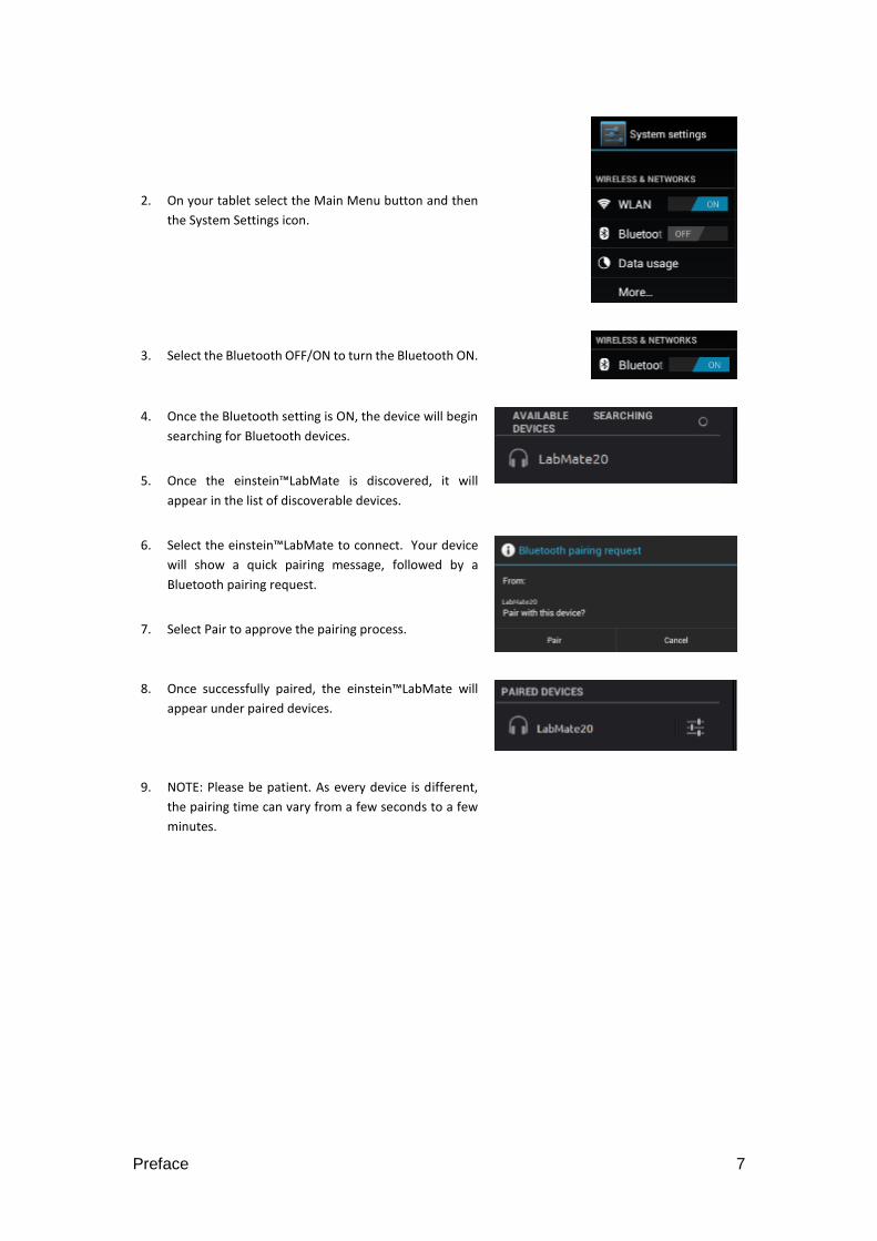
2. On your tablet select the Main Menu button and then
the System Settings icon.
3. Select the Bluetooth OFF/ON to turn the Bluetooth ON.
4. Once the Bluetooth setting is ON, the device will begin
searching for Bluetooth devices.
5. Once the einstein™LabMate is discovered, it will
appear in the list of discoverable devices.
6. Select the einstein™LabMate to connect. Your device
will show a quick pairing message, followed by a
Bluetooth pairing request.
7. Select Pair to approve the pairing process.
8. Once successfully paired, the einstein™LabMate will
appear under paired devices.
9. NOTE: Please be patient. As every device is different,
the pairing time can vary from a few seconds to a few
minutes.

Preface 8
1. On the Android device, select the Main Menu button >
System Settings icon > Bluetooth.
2. Select the icon next to einstein™LabMate that is listed
under Paired Devices.
3. A new window will appear showing, Rename and Unpair.
Select Unpair.
1. Make sure the einstein™LabMate is on and not paired with any
other device.
2. Select Settings.
3. Select the Bluetooth OFF/ON to turn the Bluetooth ON.
4. Once the Bluetooth setting is ON, the device will begin
searching for Bluetooth devices.
5. Once the einstein™LabMate is discovered, it will appear in the
list of discoverable devices.
6. Select the einstein™LabMate to connect.
7. Once successfully paired, the word Connected will appear next
to the einstein™ Lab Mate.
Preface 9
1. Select Settings.
2. Select the paired einstein™LabMate.
The experiments in this book require the use of the MiLAB program to analyze the results.
In general graphs in MiLAB represent the data from one or more sensors along the y (or vertical) axis vs.
time along the x (horizontal) axis.
By default, graphs in MiLAB auto scale which means you can see the entire graph displayed.
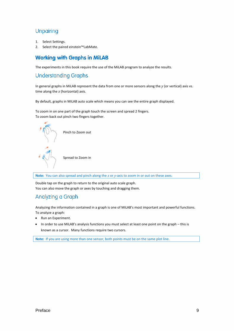
To zoom in on one part of the graph touch the screen and spread 2 fingers.
To zoom back out pinch two fingers together.
Pinch to Zoom out
Spread to Zoom in
Note: You can also spread and pinch along the x or y-axis to zoom in or out on these axes.
Double tap on the graph to return to the original auto scale graph.
You can also move the graph or axes by touching and dragging them.
Analyzing the information contained in a graph is one of MiLAB’s most important and powerful functions.
To analyze a graph:
Run an Experiment.
In order to use MiLAB’s analysis functions you must select at least one point on the graph – this is
known as a cursor. Many functions require two cursors.
Note: If you are using more than one sensor, both points must be on the same plot line.
Preface 10
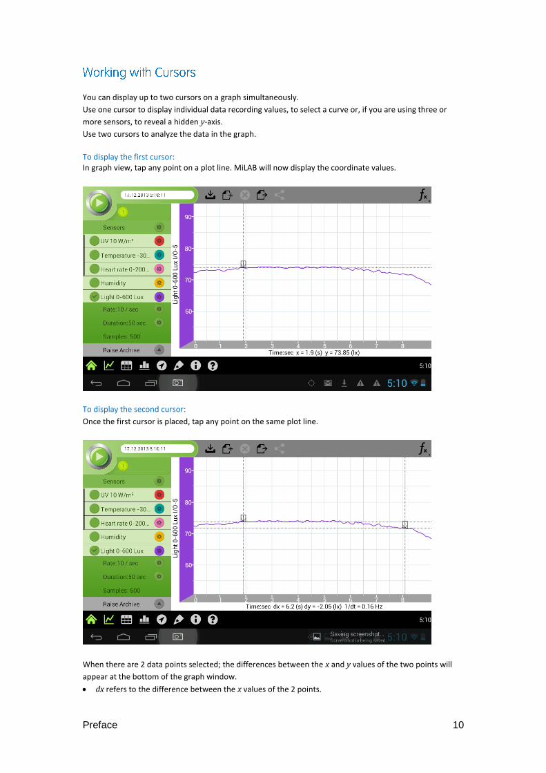
You can display up to two cursors on a graph simultaneously.
Use one cursor to display individual data recording values, to select a curve or, if you are using three or
more sensors, to reveal a hidden y-axis.
Use two cursors to analyze the data in the graph.
To display the first cursor: In graph view, tap any point on a plot line. MiLAB will now display the coordinate values.
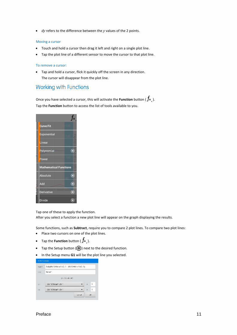
To display the second cursor:
Once the first cursor is placed, tap any point on the same plot line.
When there are 2 data points selected; the differences between the x and y values of the two points will
appear at the bottom of the graph window.
dx refers to the difference between the x values of the 2 points.
Preface 11
dy refers to the difference between the y values of the 2 points.
Moving a cursor
Touch and hold a cursor then drag it left and right on a single plot line.
Tap the plot line of a different sensor to move the cursor to that plot line.
To remove a cursor:
Tap and hold a cursor, flick it quickly off the screen in any direction.
The cursor will disappear from the plot line.
Once you have selected a cursor, this will activate the Function button ( ).
Tap the Function button to access the list of tools available to you.
Tap one of these to apply the function.
After you select a function a new plot line will appear on the graph displaying the results.
Some functions, such as Subtract, require you to compare 2 plot lines. To compare two plot lines:
Place two cursors on one of the plot lines.
Tap the Function button ( ).
Tap the Setup button ( ) next to the desired function.
In the Setup menu G1 will be the plot line you selected.
Preface 12
Use the G2 dropdown menu to select the plot line you would like to compare it to.
Tap OK.
A new plot line will appear on the graph displaying the results.
Many of the experiments in this book, especially those involving pressure measurements are dependent on
the flasks or test tubes being tightly sealed. Following is a guide to ensure that these experiments run
smoothly.
Note: To ensure a tight seal you may need to use a material such as modeling clay to seal any openings.
Note: You may want to consider purchasing the einstein™ Pressure Kit which is specifically designed for
these types of experiments.
Once you have sealed the flask or test tube, you can test the seal.
1. Tap Play ( ) to begin recording data.
2. (If your setup includes three-way valves) Turn the three-way valves to enable free air flow from the
surrounding air.
The readings should now indicate the atmospheric pressure.
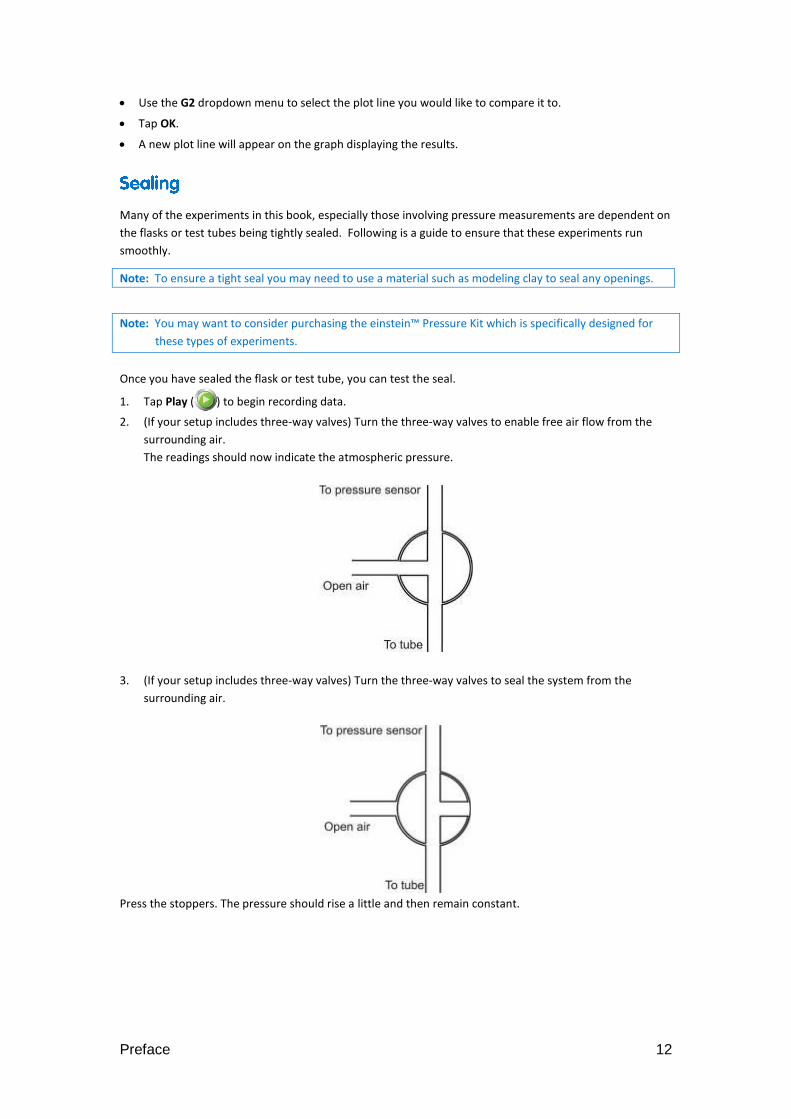
3. (If your setup includes three-way valves) Turn the three-way valves to seal the system from the
surrounding air.
Press the stoppers. The pressure should rise a little and then remain constant.
Preface 13
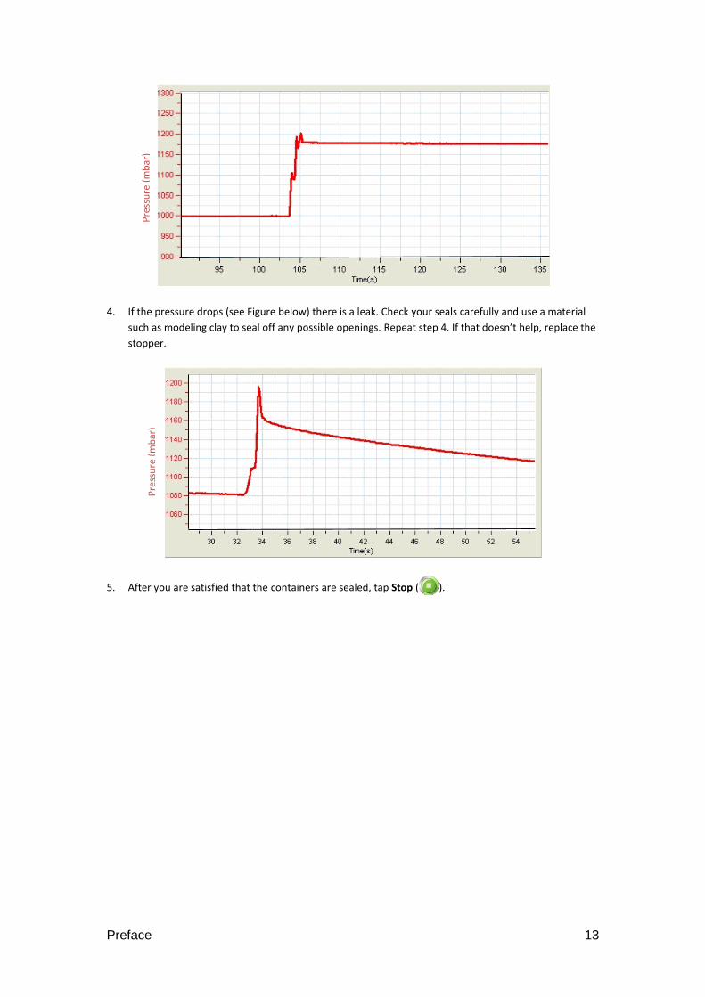
4. If the pressure drops (see Figure below) there is a leak. Check your seals carefully and use a material
such as modeling clay to seal off any possible openings. Repeat step 4. If that doesn’t help, replace the
stopper.
5. After you are satisfied that the containers are sealed, tap Stop ( ).
Pre
ssu
re (
mb
ar)
P
ress
ure
(m
bar
)

Preface 14
Each experiment includes the following parts:
Introduction: A brief description of the concept and theory
Equipment: The equipment needed for the experiment
Equipment Setup Procedure: Illustrated guide to assembling the experiment
Experimental Setup: Recommended setup
Procedure: Step-by-step guide to executing the experiment
Data Analysis
Questions
Further Suggestions
Follow standard safety procedures for laboratory activities in a science classroom.
Proper safety precautions must be taken to protect teachers and students during the experiments
described in this book.
It is not possible to include every safety precaution or warning!
Fourier assumes no responsibility or liability for use of the equipment, materials, or descriptions in
this book.
| Motion Graph Matching |
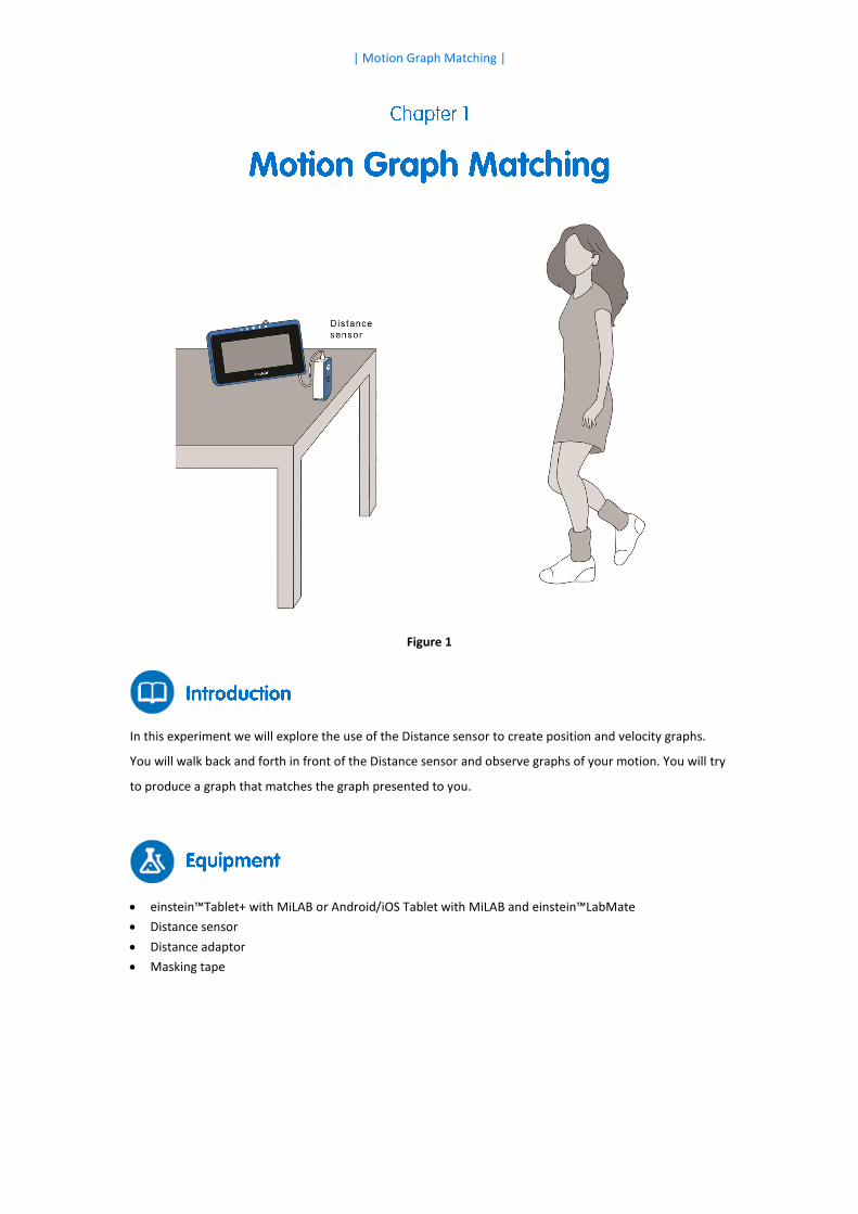
Figure 1
In this experiment we will explore the use of the Distance sensor to create position and velocity graphs.
You will walk back and forth in front of the Distance sensor and observe graphs of your motion. You will try
to produce a graph that matches the graph presented to you.
einstein™Tablet+ with MiLAB or Android/iOS Tablet with MiLAB and einstein™LabMate
Distance sensor
Distance adaptor
Masking tape
| Motion Graph Matching |
| 16 |
Note: Ensure that the AC/DC adapter is connected as the Distance sensor consumes relatively high current
1. Launch MiLAB ( ).
2. Connect the Distance sensor with the Distance adaptor to one of the ports on the einstein™Tablet+ or
einstein™LabMate.
3. Make sure that only the Distance sensor is selected.
Program the sensors to log data according to the following setup:
Distance sensor Distance (outgoing) (m)
Rate: 10/sec
Duration: 2 Min
1. Place the Distance sensor on a table so that it points toward an open space which is at least 4 m long
(see Figure 1).
2. Use short strips of masking tape on the floor to mark the 1 m, 2 m, 3 m, and 4 m positions from the
Distance sensor.
3. Produce a graph of your motion when you walk away from the Distance sensor with constant velocity.
To do this, stand about 1 m from the Distance sensor and have your lab partner tap Run ( ) to
begin recording data. Walk slowly away from the Distance sensor.
4. When you reach the 3 m mark, ask you partner to tap Stop ( ).
5. Tap Save ( ) to save your data.
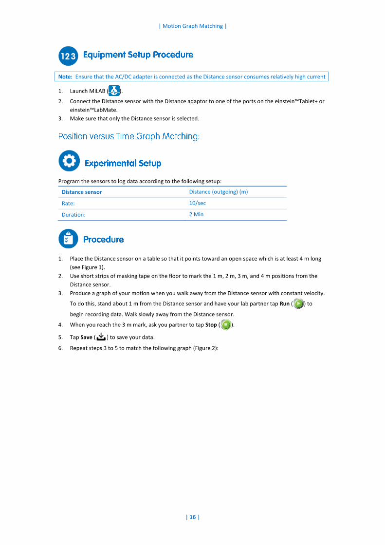
6. Repeat steps 3 to 5 to match the following graph (Figure 2):
| Motion Graph Matching |
| 17 |
Figure 2: Position vs. Time graph
Program the sensor to log data according to the following setup:
Distance sensor Velocity (outgoing) (m/s)
Rate: 10/sec
Duration: 2 Min
1. Place the Distance sensor on a table so that it points toward an open space which is at least 4 m long
(see Figure 1).
2. Use short strips of masking tape on the floor to mark the 1 m, 2 m, 3 m, and 4 m positions from the
Distance sensor.
3. Produce a graph of your motion when you walk away from the Distance sensor with constant velocity.
To do this, stand about 1 m from the Distance sensor and have your Lab partner select Run ( ) to
begin recording data. Walk slowly away from the Distance sensor.
4. When you reach the 3 m mark, ask your partner to select Stop ( ).
5. Tap Save ( ) to save your data.
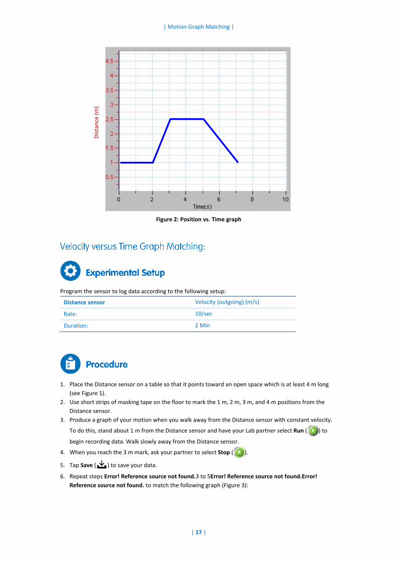
6. Repeat steps Error! Reference source not found.3 to 5Error! Reference source not found.Error!
Reference source not found. to match the following graph (Figure 3):
Dis
tan
ce (
m)
| Motion Graph Matching |
| 18 |
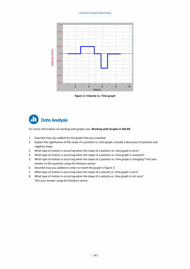
Figure 3: Velocity vs. Time graph
For more information on working with graphs see: Working with Graphs in MiLAB.
1. Describe how you walked for the graph that you matched.
2. Explain the significance of the slope of a position vs. time graph. Include a discussion of positive and
negative slope.
3. What type of motion is occurring when the slope of a position vs. time graph is zero?
4. What type of motion is occurring when the slope of a position vs. time graph is constant?
5. What type of motion is occurring when the slope of a position vs. time graph is changing? Test your
answer to this question using the Distance sensor.
6. Describe how you walked in order to match the graph in Figure 3.
7. What type of motion is occurring when the slope of a velocity vs. time graph is zero?
8. What type of motion is occurring when the slope of a velocity vs. time graph is not zero?
Test your answer using the Distance sensor.
Vel
oci
ty (
m/s
)
| Position and Velocity Measurements |
| 19 |
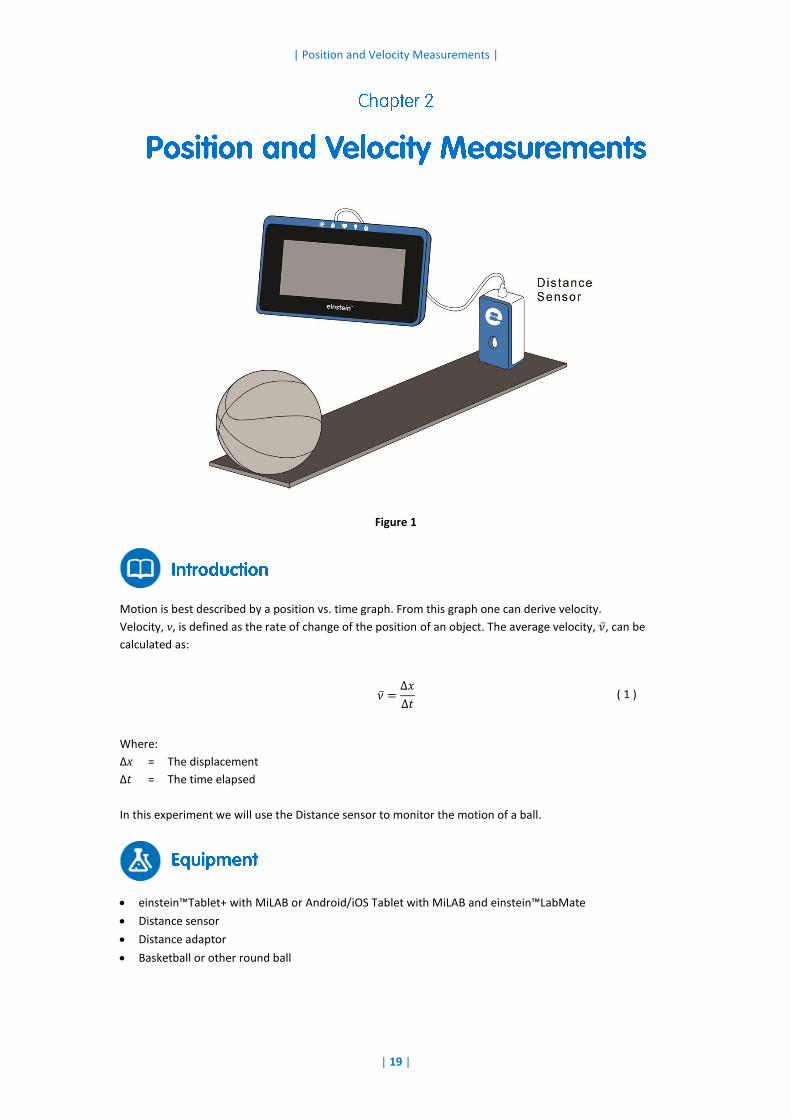
Figure 1
Motion is best described by a position vs. time graph. From this graph one can derive velocity.
Velocity, v, is defined as the rate of change of the position of an object. The average velocity, �̅�, can be
calculated as:
�̅� =Δ𝑥
Δ𝑡 ( 1 )
Where:
Δx = The displacement
Δt = The time elapsed
In this experiment we will use the Distance sensor to monitor the motion of a ball.
einstein™Tablet+ with MiLAB or Android/iOS Tablet with MiLAB and einstein™LabMate
Distance sensor
Distance adaptor
Basketball or other round ball
| Position and Velocity Measurements |
| 20 |
1. Launch MiLAB ( ).
2. Connect the Distance sensor with the Distance adaptor to one of the ports on the einstein™Tablet+ or
einstein™LabMate.
3. Make sure only the Distance sensor is selected.
Program the sensors to log data according to the following setup:
Distance sensor Distance (outgoing) (m)
Rate: 10/sec
Duration: 2 Min
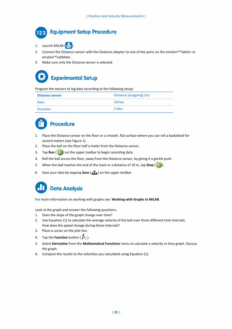
1. Place the Distance sensor on the floor or a smooth, flat surface where you can roll a basketball for
several meters (see Figure 1).
2. Place the ball on the floor half a meter from the Distance sensor.
3. Tap Run ( ) on the upper toolbar to begin recording data.
4. Roll the ball across the floor, away from the Distance sensor, by giving it a gentle push.
5. When the ball reaches the end of the track or a distance of 10 m, tap Stop ( ).
6. Save your data by tapping Save ( ) on the upper toolbar.
For more information on working with graphs see: Working with Graphs in MiLAB.
Look at the graph and answer the following questions:
1. Does the slope of the graph change over time?
2. Use Equation (1) to calculate the average velocity of the ball over three different time intervals.
How does the speed change during those intervals?
3. Place a cursor on the plot line.
4. Tap the Function button ( ).
5. Select Derivative from the Mathematical Functions menu to calculate a velocity vs time graph. Discuss
the graph.
6. Compare the results to the velocities you calculated using Equation (1).
| Motion on an Inclined Plane |
| 21 |
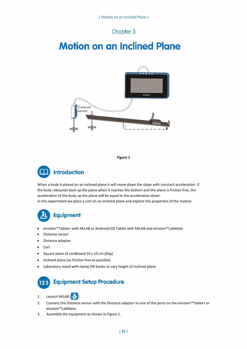
Figure 1
When a body is placed on an inclined plane it will move down the slope with constant acceleration. If
the body rebounds back up the plane when it reaches the bottom and the plane is friction free, the
acceleration of the body up the plane will be equal to the acceleration down.
In this experiment we place a cart on an inclined plane and explore the properties of the motion.
einstein™Tablet+ with MiLAB or Android/iOS Tablet with MiLAB and einstein™LabMate
Distance sensor
Distance adaptor
Cart
Square piece of cardboard 10 x 10 cm (flag)
Inclined plane (as friction free as possible)
Laboratory stand with clamp OR books to vary height of inclined plane
1. Launch MiLAB ( ).
2. Connect the Distance sensor with the Distance adaptor to one of the ports on the einstein™Tablet+ or
einstein™LabMate.
3. Assemble the equipment as shown in Figure 1.
| Motion on an Inclined Plane |
| 22 |
4. Place the Distance sensor at the upper end of the inclined plane.
5. Place a stopper at the bottom of the plane.
6. The starting distance between the cart and the Distance sensor should be at least 50 cm.
7. Make sure that only the Distance sensor is selected.
Program the sensors to log data according to the following setup:
Distance sensor Distance (outgoing) (m)
Rate: 10/sec
Duration: 10 Sec
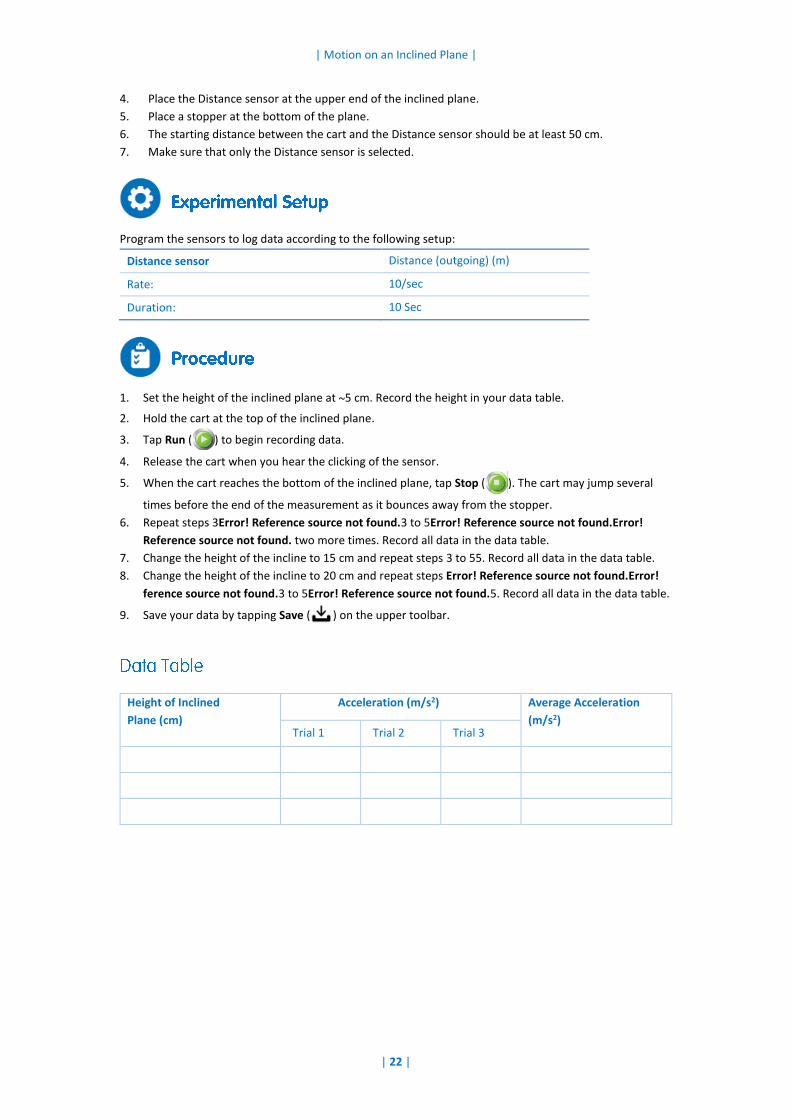
1. Set the height of the inclined plane at ~5 cm. Record the height in your data table.
2. Hold the cart at the top of the inclined plane.
3. Tap Run ( ) to begin recording data.
4. Release the cart when you hear the clicking of the sensor.
5. When the cart reaches the bottom of the inclined plane, tap Stop ( ). The cart may jump several
times before the end of the measurement as it bounces away from the stopper.
6. Repeat steps 3Error! Reference source not found.3 to 5Error! Reference source not found.Error!
Reference source not found. two more times. Record all data in the data table.
7. Change the height of the incline to 15 cm and repeat steps 3 to 55. Record all data in the data table.
8. Change the height of the incline to 20 cm and repeat steps Error! Reference source not found.Error!
ference source not found.3 to 5Error! Reference source not found.5. Record all data in the data table.
9. Save your data by tapping Save ( ) on the upper toolbar.
Height of Inclined
Plane (cm)
Acceleration (m/s2) Average Acceleration
(m/s2) Trial 1 Trial 2 Trial 3
| Motion on an Inclined Plane |
| 23 |
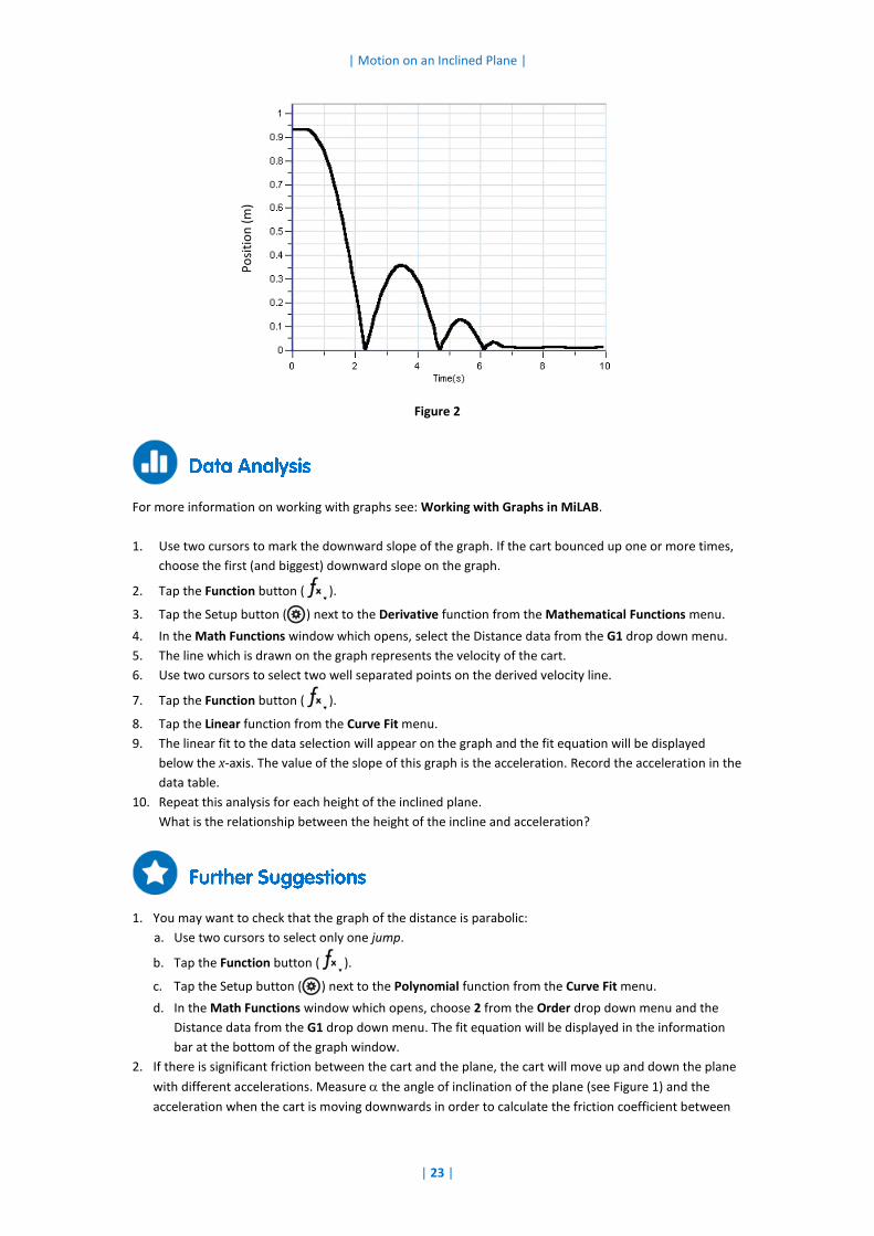
Figure 2
For more information on working with graphs see: Working with Graphs in MiLAB.
1. Use two cursors to mark the downward slope of the graph. If the cart bounced up one or more times,
choose the first (and biggest) downward slope on the graph.
2. Tap the Function button ( ).
3. Tap the Setup button ( ) next to the Derivative function from the Mathematical Functions menu.
4. In the Math Functions window which opens, select the Distance data from the G1 drop down menu.
5. The line which is drawn on the graph represents the velocity of the cart.
6. Use two cursors to select two well separated points on the derived velocity line.
7. Tap the Function button ( ).
8. Tap the Linear function from the Curve Fit menu.
9. The linear fit to the data selection will appear on the graph and the fit equation will be displayed
below the x-axis. The value of the slope of this graph is the acceleration. Record the acceleration in the
data table.
10. Repeat this analysis for each height of the inclined plane.
What is the relationship between the height of the incline and acceleration?
1. You may want to check that the graph of the distance is parabolic:
a. Use two cursors to select only one jump.
b. Tap the Function button ( ).
c. Tap the Setup button ( ) next to the Polynomial function from the Curve Fit menu.
d. In the Math Functions window which opens, choose 2 from the Order drop down menu and the
Distance data from the G1 drop down menu. The fit equation will be displayed in the information
bar at the bottom of the graph window.
2. If there is significant friction between the cart and the plane, the cart will move up and down the plane
with different accelerations. Measure the angle of inclination of the plane (see Figure 1) and the
acceleration when the cart is moving downwards in order to calculate the friction coefficient between
Po
siti
on
(m
)

| Motion on an Inclined Plane |
| 24 |
the cart and the plane:
𝜇 =𝑔 sin 𝛼 − 𝑎𝑑𝑜𝑤𝑛
𝑔 cos 𝛼
3. Start the motion of the cart at different points on the plane and in different directions and try to predict
the shapes of the distance and velocity graphs.
4. Place the sensor at the upper end of the inclined plane and try to predict in advance the form of the
graphs of distance and velocity.
| Friction Coefficient |
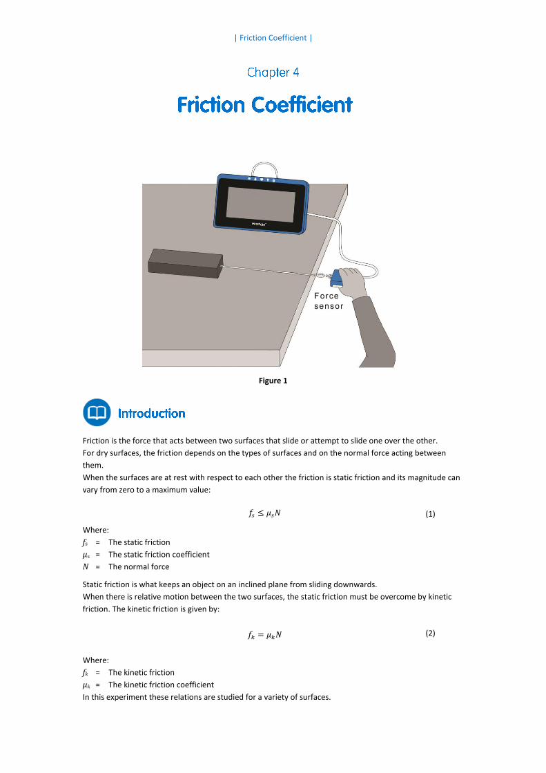
Figure 1
Friction is the force that acts between two surfaces that slide or attempt to slide one over the other.
For dry surfaces, the friction depends on the types of surfaces and on the normal force acting between
them.
When the surfaces are at rest with respect to each other the friction is static friction and its magnitude can
vary from zero to a maximum value:
𝑓𝑠 ≤ 𝜇𝑠𝑁 (1)
Where:
fs = The static friction
µs = The static friction coefficient
N = The normal force
Static friction is what keeps an object on an inclined plane from sliding downwards.
When there is relative motion between the two surfaces, the static friction must be overcome by kinetic
friction. The kinetic friction is given by:
𝑓𝑘 = 𝜇𝑘𝑁 (2)
Where:
fk = The kinetic friction
µk = The kinetic friction coefficient
In this experiment these relations are studied for a variety of surfaces.
| Friction Coefficient |
| 26 |
einstein™Tablet+ with MiLAB or Android/iOS Tablet with MiLAB and einstein™LabMate
Force sensor
Blocks of several materials (e.g. wooden block and a brick)
String
Balance to measure the mass of the blocks
1. Launch MiLAB ( ).
2. Connect the Force sensor to one of the ports on the einstein™Tablet+ or einstein™LabMate.
3. Assemble the equipment as shown in Figure 1.
4. Attach one end of the string to the block.
5. Attach the other end of the string to the Force sensor so that pulling the sensor will drag the block
along the table or other surface. The Force sensor will measure the force acting on the block.
6. Make sure that only the Force sensor is selected.
Program the sensor to log data according to the following setup:
Force sensor Force, Pull – positive (10 or 50 N) (N)
Set As Zero ON
Rate: 10/sec
Duration: 2 Min
1. Measure the mass of each block of material and record the measurements in your notebook.
2. Select Run ( ) to begin recording data.
3. Place the block on a table or other surface.
4. Hold the Force sensor in your hand and pull it. Make sure that the string is horizontal to the surface on
which the block is resting and gradually increase the applied force. When the block starts moving,
maintain a constant velocity. Only when the block moves at constant velocity is the friction exactly
balanced by the force acting on the block.
5. When you have pulled the block a short distance, select Stop ( ).
6. Save your data by tapping Save ( ) on the upper toolbar.
7. Repeat the experiment with different materials. Remember to save the data from each experiment
with a unique name.
| Friction Coefficient |
| 27 |
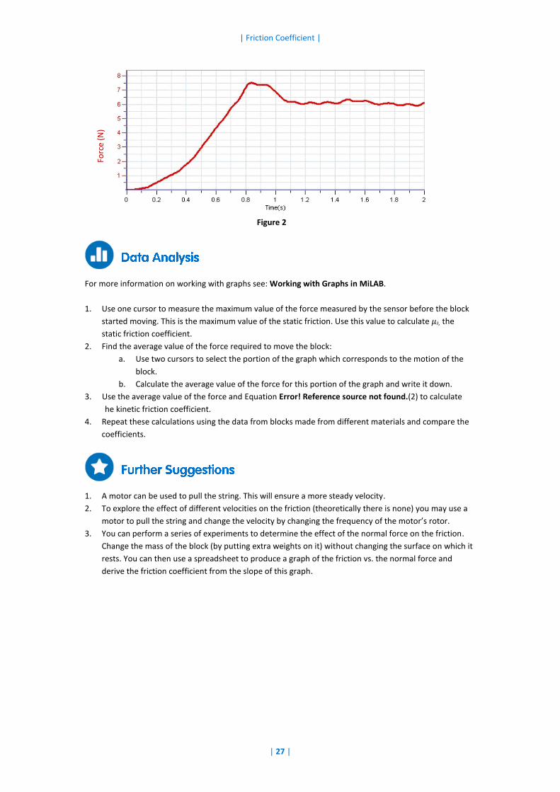
Figure 2
For more information on working with graphs see: Working with Graphs in MiLAB.
1. Use one cursor to measure the maximum value of the force measured by the sensor before the block
started moving. This is the maximum value of the static friction. Use this value to calculate µs, the
static friction coefficient.
2. Find the average value of the force required to move the block:
a. Use two cursors to select the portion of the graph which corresponds to the motion of the
block.
b. Calculate the average value of the force for this portion of the graph and write it down.
3. Use the average value of the force and Equation Error! Reference source not found.(2) to calculate
he kinetic friction coefficient.
4. Repeat these calculations using the data from blocks made from different materials and compare the
coefficients.
1. A motor can be used to pull the string. This will ensure a more steady velocity.
2. To explore the effect of different velocities on the friction (theoretically there is none) you may use a
motor to pull the string and change the velocity by changing the frequency of the motor’s rotor.
3. You can perform a series of experiments to determine the effect of the normal force on the friction.
Change the mass of the block (by putting extra weights on it) without changing the surface on which it
rests. You can then use a spreadsheet to produce a graph of the friction vs. the normal force and
derive the friction coefficient from the slope of this graph.
Forc
e (N
)
| Newton's Third Law|
Figure 1
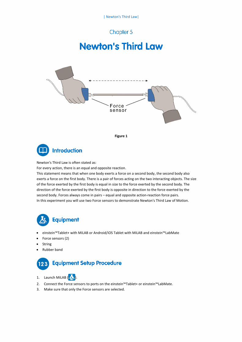
Newton's Third Law is often stated as:
For every action, there is an equal and opposite reaction.
This statement means that when one body exerts a force on a second body, the second body also
exerts a force on the first body. There is a pair of forces acting on the two interacting objects. The size
of the force exerted by the first body is equal in size to the force exerted by the second body. The
direction of the force exerted by the first body is opposite in direction to the force exerted by the
second body. Forces always come in pairs – equal and opposite action-reaction force pairs.
In this experiment you will use two Force sensors to demonstrate Newton's Third Law of Motion.
einstein™Tablet+ with MiLAB or Android/iOS Tablet with MiLAB and einstein™LabMate
Force sensors (2)
String
Rubber band
1. Launch MiLAB ( ).
2. Connect the Force sensors to ports on the einstein™Tablet+ or einstein™LabMate.
3. Make sure that only the Force sensors are selected.
| Newton's Third Law |
| 29 |
Program the sensors to log data according to the following setup:
Force sensor Force, Pull – positive (50 N) (N)
Set As Zero ON
Rate: 10/sec
Duration: 50 Sec
1. Tie the two Force sensors together with a string about 20 cm long. Hold one Force sensor in your hand
and have your partner hold the other Force sensor so you can pull on each other (see Figure 1).
2. Tap Run ( ) on the upper toolbar to begin recording data.
3. Gently tug on your partner’s Force sensor with your Force sensor, making sure the graph does not go
off the scale. Also, have your partner tug on your sensor. You will have 50 seconds to try different pulls.
4. Save your data by tapping Save ( ) on the upper toolbar.
5. Repeat the experiment with different materials. Remember to save the data from each experiment
with a unique name.
6. What would happen if you used the rubber band instead of the string? Make a prediction using the
Predict tool.
a. Open the Setup window ( ) from the Sensor Control Panel.
b. Turn on the Predict tool and close the setup window. Tap the Predict tool ( ) and follow
the instruction to sketch a prediction on the graph.
c. Repeat steps 2-4Error! Reference source not found. using the rubber band instead of the
string.
For more information on working with graphs see: Working with Graphs in MiLAB.
1. Examine the graphs.
a. What can you conclude about the two forces (your pull on your partner and your partner’s
pull on you)?
b. How are the magnitudes related?
c. How are the signs related?
2. How does the rubber band change the results - or does it change them at all?
3. While you and your partner are pulling on each other’s Force sensors, do your Force sensors have the
same positive direction? What impact does your answer have on the analysis of the force pair?
4. Is there any way to pull on your partner’s Force sensor without your partner’s Force sensor pulling
back? Try it.
1. Fasten one Force sensor to your Lab bench and repeat the experiment. Does the bench pull back as
you pull on it? Does it matter that the second force sensor is not held by a person?

| Newton's Third Law |
| 30 |
2. Use a rigid rod to connect your Force sensors instead of a string and experiment with mutual pushes
instead of pulls. Repeat the experiment. Does the rod change the way the force pairs are related?
| The Impact of Constant Force
on a Moving Body |
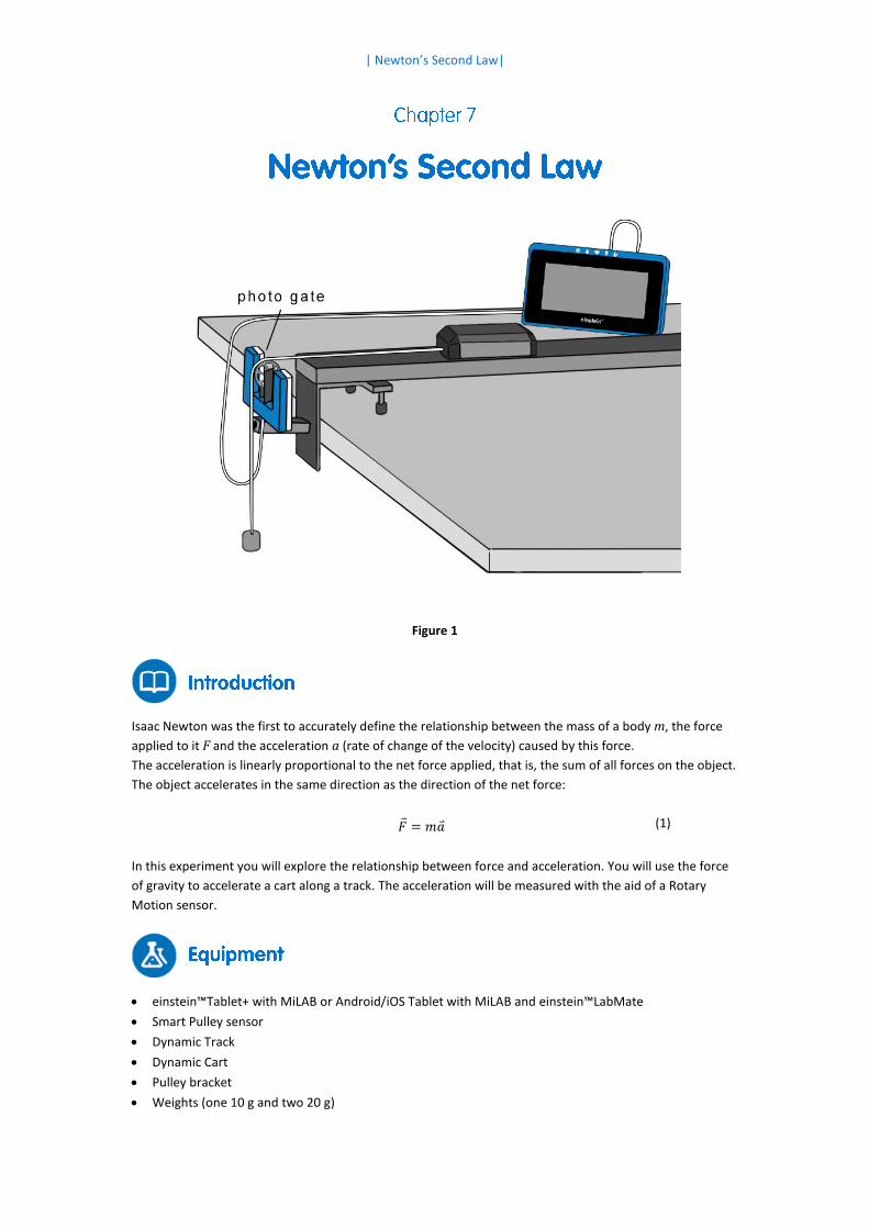
Figure 1
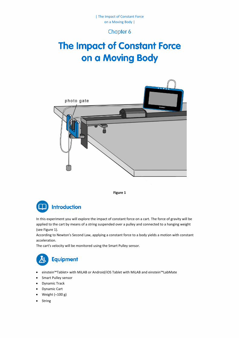
In this experiment you will explore the impact of constant force on a cart. The force of gravity will be
applied to the cart by means of a string suspended over a pulley and connected to a hanging weight
(see Figure 1).
According to Newton's Second Law, applying a constant force to a body yields a motion with constant
acceleration.
The cart's velocity will be monitored using the Smart Pulley sensor.
einstein™Tablet+ with MiLAB or Android/iOS Tablet with MiLAB and einstein™LabMate
Smart Pulley sensor
Dynamic Track
Dynamic Cart
Weight (~100 g)
String
| The Impact of Constant Force on a Moving Body |
| 32 |
1. Launch MiLAB ( ).
2. Assemble the Smart Pulley sensor by mounting the pulley on the Photogate sensor with the rod
provided.
3. Mount the Smart Pulley sensor on one end of the track using the pulley mounting bracket.
4. Connect the Smart Pulley sensor to one of the ports on the einstein™Tablet+ or einstein™LabMate.
5. Position the cart at the other end of the track.
6. Attach a string to the cart.
7. Attach a 100 g weight to the other end of the string.
8. Pass the string over the pulley.
9. Level the track and adjust the Smart Pulley height so that the string is parallel to the track.
10. Make sure that only the Smart Pulley sensor is selected.
Program the sensors to log data according to the following setup:
Smart Pulley Sensor
Rate: 25/sec
Duration: 4 Sec
Note: Make sure that only the Smart Pulley is selected and not the Photogate.
1. Hold the cart at the end of the track.
2. Tap Run ( ) on the upper toolbar.
3. Release the cart.
4. Tap Stop ( ) on the upper toolbar as the hanging mass reaches the floor.
5. Save your data by tapping Save ( ) on the upper toolbar.
| The Impact of Constant Force on a Moving Body |
| 33 |
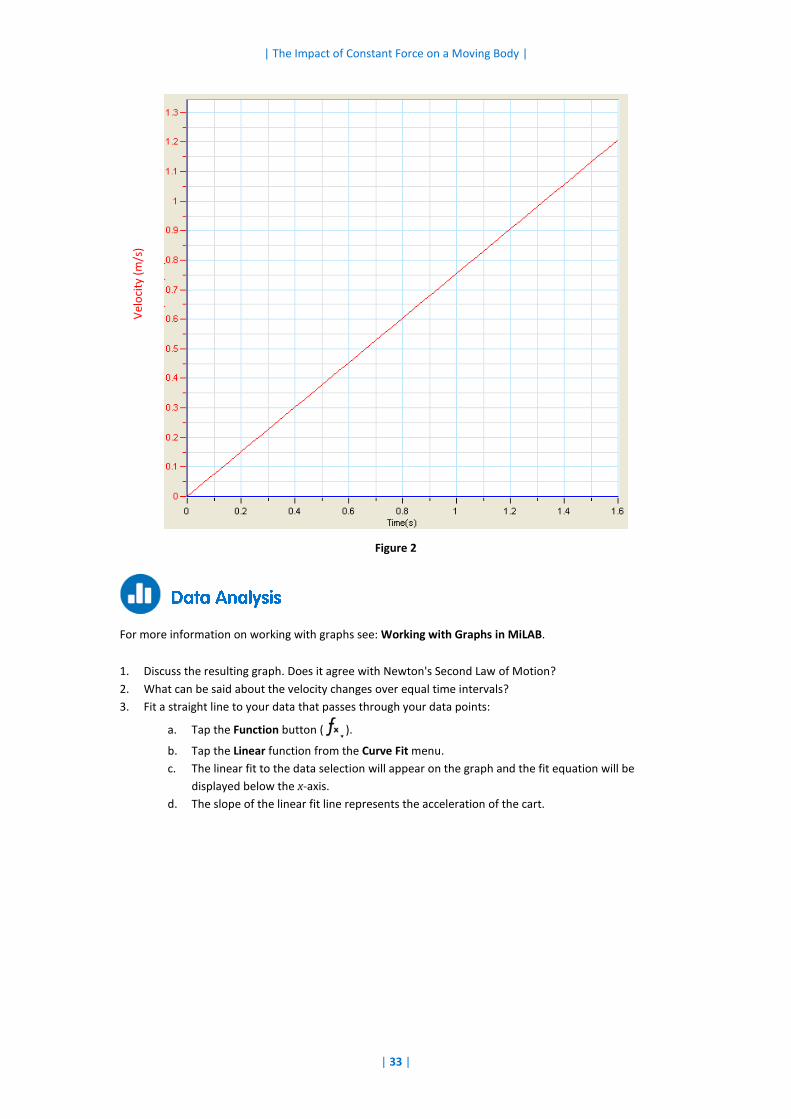
Figure 2
For more information on working with graphs see: Working with Graphs in MiLAB.
1. Discuss the resulting graph. Does it agree with Newton's Second Law of Motion?
2. What can be said about the velocity changes over equal time intervals?
3. Fit a straight line to your data that passes through your data points:
a. Tap the Function button ( ).
b. Tap the Linear function from the Curve Fit menu.
c. The linear fit to the data selection will appear on the graph and the fit equation will be
displayed below the x-axis.
d. The slope of the linear fit line represents the acceleration of the cart.
Vel
oci
ty (
m/s
)
| Newton’s Second Law|
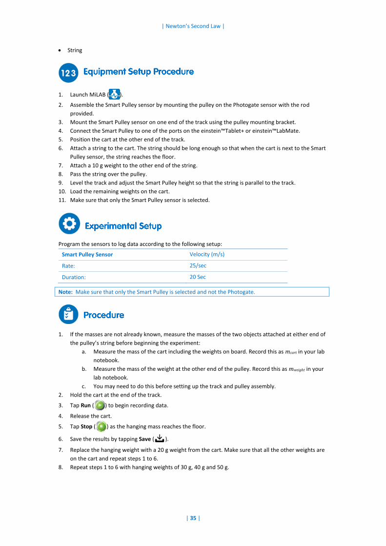
Figure 1
Isaac Newton was the first to accurately define the relationship between the mass of a body m, the force
applied to it F and the acceleration a (rate of change of the velocity) caused by this force.
The acceleration is linearly proportional to the net force applied, that is, the sum of all forces on the object.
The object accelerates in the same direction as the direction of the net force:
�⃑� = 𝑚�⃑� (1)
In this experiment you will explore the relationship between force and acceleration. You will use the force
of gravity to accelerate a cart along a track. The acceleration will be measured with the aid of a Rotary
Motion sensor.
einstein™Tablet+ with MiLAB or Android/iOS Tablet with MiLAB and einstein™LabMate
Smart Pulley sensor
Dynamic Track
Dynamic Cart
Pulley bracket
Weights (one 10 g and two 20 g)
| Newton’s Second Law |
| 35 |
String
1. Launch MiLAB ( ).
2. Assemble the Smart Pulley sensor by mounting the pulley on the Photogate sensor with the rod
provided.
3. Mount the Smart Pulley sensor on one end of the track using the pulley mounting bracket.
4. Connect the Smart Pulley to one of the ports on the einstein™Tablet+ or einstein™LabMate.
5. Position the cart at the other end of the track.
6. Attach a string to the cart. The string should be long enough so that when the cart is next to the Smart
Pulley sensor, the string reaches the floor.
7. Attach a 10 g weight to the other end of the string.
8. Pass the string over the pulley.
9. Level the track and adjust the Smart Pulley height so that the string is parallel to the track.
10. Load the remaining weights on the cart.
11. Make sure that only the Smart Pulley sensor is selected.
Program the sensors to log data according to the following setup:
Smart Pulley Sensor Velocity (m/s)
Rate: 25/sec
Duration: 20 Sec
Note: Make sure that only the Smart Pulley is selected and not the Photogate.
1. If the masses are not already known, measure the masses of the two objects attached at either end of
the pulley’s string before beginning the experiment:
a. Measure the mass of the cart including the weights on board. Record this as mcart in your lab
notebook.
b. Measure the mass of the weight at the other end of the pulley. Record this as mweight in your
lab notebook.
c. You may need to do this before setting up the track and pulley assembly.
2. Hold the cart at the end of the track.
3. Tap Run ( ) to begin recording data.
4. Release the cart.
5. Tap Stop ( ) as the hanging mass reaches the floor.
6. Save the results by tapping Save ( ).
7. Replace the hanging weight with a 20 g weight from the cart. Make sure that all the other weights are
on the cart and repeat steps 1 to 6.
8. Repeat steps 1 to 6 with hanging weights of 30 g, 40 g and 50 g.
| Newton’s Second Law |
| 36 |
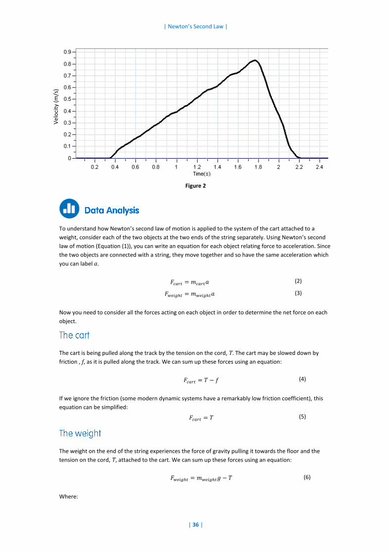
Figure 2
To understand how Newton’s second law of motion is applied to the system of the cart attached to a
weight, consider each of the two objects at the two ends of the string separately. Using Newton’s second
law of motion (Equation (1)), you can write an equation for each object relating force to acceleration. Since
the two objects are connected with a string, they move together and so have the same acceleration which
you can label a.
𝐹𝑐𝑎𝑟𝑡 = 𝑚𝑐𝑎𝑟𝑡𝑎 (2)
𝐹𝑤𝑒𝑖𝑔ℎ𝑡 = 𝑚𝑤𝑒𝑖𝑔ℎ𝑡𝑎 (3)
Now you need to consider all the forces acting on each object in order to determine the net force on each
object.
The cart is being pulled along the track by the tension on the cord, T. The cart may be slowed down by
friction , f, as it is pulled along the track. We can sum up these forces using an equation:
𝐹𝑐𝑎𝑟𝑡 = 𝑇 − 𝑓 (4)
If we ignore the friction (some modern dynamic systems have a remarkably low friction coefficient), this
equation can be simplified:
𝐹𝑐𝑎𝑟𝑡 = 𝑇 (5)
The weight on the end of the string experiences the force of gravity pulling it towards the floor and the
tension on the cord, T, attached to the cart. We can sum up these forces using an equation:
𝐹𝑤𝑒𝑖𝑔ℎ𝑡 = 𝑚𝑤𝑒𝑖𝑔ℎ𝑡𝑔 − 𝑇 (6)
Where:
Vel
oci
ty (
m/s
)
| Newton’s Second Law |
| 37 |
g = The acceleration due to gravity
Substituting this equation into the relationship already found for the tension on the string (Equation (5)):
𝐹𝑤𝑒𝑖𝑔ℎ𝑡 = 𝑚𝑤𝑒𝑖𝑔ℎ𝑡𝑔 − 𝐹𝑐𝑎𝑟𝑡 (7)
Now substituting in the original Newton’s second law of motion equations (Equations (2) and (3)):
𝑚𝑤𝑒𝑖𝑔ℎ𝑡𝑎 = 𝑚𝑤𝑒𝑖𝑔ℎ𝑡𝑔 − 𝑚𝑐𝑎𝑟𝑡𝑎 (8)
With some rearranging of this equation, you can find a relationship between the acceleration of the objects
and their masses:
𝑎 =1
𝑚𝑐𝑎𝑟𝑡 + 𝑚𝑤𝑒𝑖𝑔ℎ𝑡
∙ 𝑚𝑤𝑒𝑖𝑔ℎ𝑡𝑔 (9)
Because the total mass, mcart + mweight, remains constant, the graph of acceleration vs the applied force,
mweightg is a straight line with slope:
𝑠𝑙𝑜𝑝𝑒 =1
𝑚𝑐𝑎𝑟𝑡 + 𝑚𝑤𝑒𝑖𝑔ℎ𝑡
(10)
For more information on working with graphs see: Working with Graphs in MiLAB.
1. From the graph (Figure 2) you can see that the velocity increases linearly over time. That means that
the acceleration is constant, as the acceleration is the rate of change in velocity.
2. Use the cursors to select the linear range of the graph.
3. Tap the Function button ( ).
4. Tap the Linear function from the Curve Fit menu.
5. The linear fit equation will be displayed below the x-axis.
6. The slope of the linear fit line represents the acceleration of the cart.
7. Prepare a data table:
mweight (g) a (m/s2) F = mweightg (N)
1. Repeat the calculations for each of your saved data files and fill in the data table.
2. Graph the acceleration vs. the applied force, mweightg, and find the slope of the resulting line.
3. Compare the graph’s slope to the theoretical one (see Equation (10)).
4. Calculate the relative error:
𝑅𝑒𝑙𝑎𝑡𝑖𝑣𝑒 𝑒𝑟𝑟𝑜𝑟 (%) = |𝑇ℎ𝑒𝑜𝑟𝑒𝑡𝑖𝑐𝑎𝑙 − 𝐸𝑥𝑝𝑒𝑟𝑖𝑚𝑒𝑛𝑡𝑎𝑙
𝑇ℎ𝑒𝑜𝑟𝑒𝑡𝑖𝑐𝑎𝑙| × 100%

| Newton’s Second Law |
| 38 |
If there is a significant friction in your system, find the friction coefficient from the graph.
| Energy of a Tossed Ball |
| 39 |
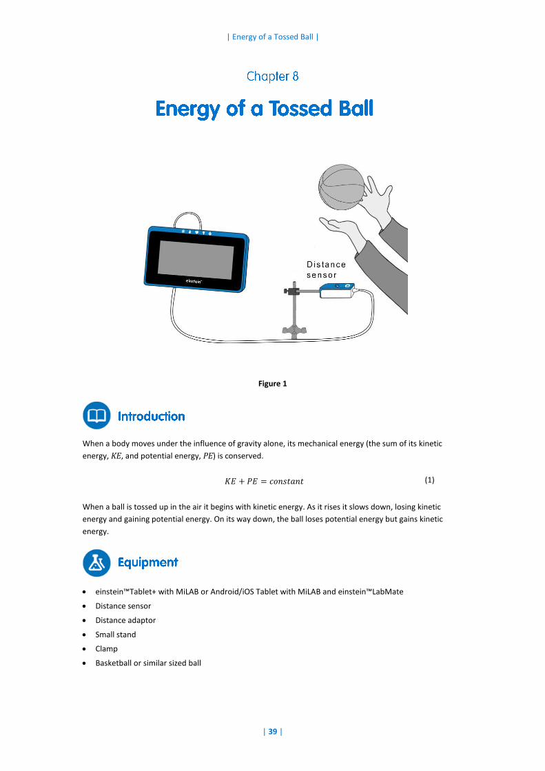
Figure 1
When a body moves under the influence of gravity alone, its mechanical energy (the sum of its kinetic
energy, KE, and potential energy, PE) is conserved.
𝐾𝐸 + 𝑃𝐸 = 𝑐𝑜𝑛𝑠𝑡𝑎𝑛𝑡 (1)
When a ball is tossed up in the air it begins with kinetic energy. As it rises it slows down, losing kinetic
energy and gaining potential energy. On its way down, the ball loses potential energy but gains kinetic
energy.
einstein™Tablet+ with MiLAB or Android/iOS Tablet with MiLAB and einstein™LabMate
Distance sensor
Distance adaptor
Small stand
Clamp
Basketball or similar sized ball
| Energy of a Tossed Ball |
| 40 |
1. Measure and record the mass of the ball.
2. Launch MiLAB ( ).
3. Connect the Distance sensor with the Distance adaptor to one of the ports on the einstein™LabMate.
4. Assemble the equipment as shown in Figure 1.
5. Make sure that only the Distance sensor is selected.
Program the sensor to log data according to the following setup:
Distance Sensor Distance (m)
Rate: 25/sec
Duration: 20 Sec
1. Using two hands, practice tossing the ball straight up. The range should be from about 0.5 m above the
Distance sensor to about 1.5 m above the Distance sensor.
2. Tap Run ( ) to begin recording data.
3. When you hear the clicking sound of the Distance sensor, toss the ball and move your hands out of the
way.
4. Catch the ball when it is comes back to about 0.5 m above the Distance sensor.
5. Tap Stop ( ).
6. Save the results by tapping Save ( ).
For more information on working with graphs see: Working with Graphs in MiLAB.
1. Display a graph of the Velocity by taking the derivative of the distance vs time graph:
a. Tap the Function button ( ).
b. Tap the Setup button ( ) next to the Derivative function from the Mathematical Functions
menu.
c. In the G1 drop down menu select the Distance data.
d. The line which is drawn on the graph represents the velocity of the cart.
2. Use the velocity data to calculate the kinetic energy of the ball:
a. Tap the Function button ( ).
b. Tap the Setup button ( ) next to the Square function from the Mathematical Functions menu.
c. In the Math Functions window which opens, select the calculated velocity data from the G1
drop down menu.

| Energy of a Tossed Ball |
| 41 |
d. In the A edit box, enter half the value of the mass of the ball.
e. Type KE in the Name edit box; type J in the Unit edit box.
1. Use the cursor to select the Distance data:
a. Tap the Function button ( ).
b. Tap the Setup button ( ) next to the Linear function from the Mathematical Functions menu.
c. In the Math Functions window which opens, select the Distance data from the G1 drop down
menu.
d. In the A edit box, enter the result of the mass of the ball multiplied by the free fall acceleration
(9.8 m/s2).
e. In the B edit box enter 0.
f. Type PE in the Name edit box; type J in the Unit edit box.
1. Export the data ( ) as a .csv file.
2. Create a plot of Potential Energy vs Kinetic Energy.
3. Discuss the graph in terms of the transitions between potential and kinetic energy and conservation of
energy.
| Hooke’s Law:
Finding the Spring Constant |
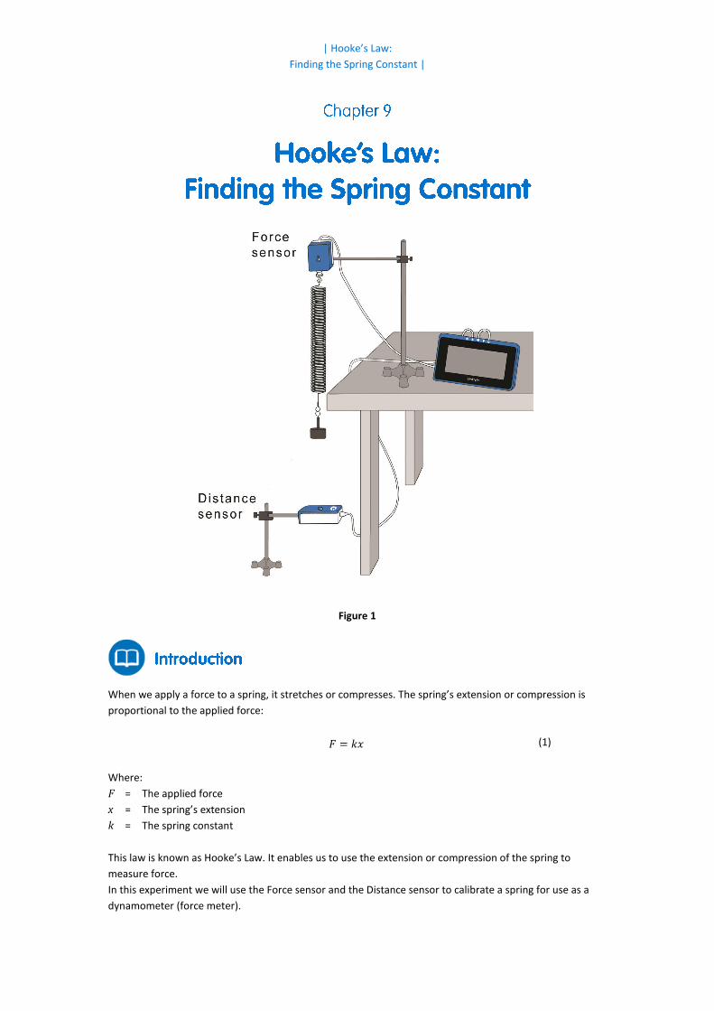
Figure 1
When we apply a force to a spring, it stretches or compresses. The spring’s extension or compression is
proportional to the applied force:
𝐹 = 𝑘𝑥 (1)
Where:
F = The applied force
x = The spring’s extension
k = The spring constant
This law is known as Hooke’s Law. It enables us to use the extension or compression of the spring to
measure force.
In this experiment we will use the Force sensor and the Distance sensor to calibrate a spring for use as a
dynamometer (force meter).
| Hooke’s Law: Finding the Spring Constant |
| 43 |
einstein™Tablet+ with MiLAB or Android/iOS Tablet with MiLAB and einstein™LabMate
Force sensor
Distance sensor
Distance adaptor
Spring (~15 N/m)
Slotted mass set
Slotted mass hanger
Stand and supporting rod (2)
Clamp with hook to hang the spring
1. Launch MiLAB ( ).
2. Connect the Distance sensor with the Distance adaptor to one of the ports on the einstein™Tablet+ or
einstein™LabMate.
3. Connect the Force sensor to one of the ports on the einstein™Tablet+ or einstein™LabMate.
4. Assemble the equipment as shown in Figure 1.
a. Make sure there are no physical obstacles between the hanging mass and the Distance sensor.
b. Use a mass of 100 g.
c. The distance between the mass and sensor should be about 70 cm.
5. Make sure that the Distance sensor and the Force sensor are the only sensors selected.
Program the sensors to log data according to the following setup:
Distance Sensor Distance (m)
Force Sensor Force, Pull - positive ( 10 N) (N)
Set As Zero ON
Rate: 10 samples/ sec
Duration: 2 Min
1. Make sure that the hanging mass is at rest.
2. Tap Run ( ) on the upper toolbar to begin recording data.
3. Wait 20 seconds and then add a weight of 50 g to the hanging mass so that the total mass is now
150 g. Bring the mass to rest.
4. Wait another 20 seconds then add again a mass of 50 g and bring the mass to rest.
5. Repeat step 4 and increase the hanging mass by amounts of 50 g until you reach 500 g.
6. Tap Stop ( ).
7. Save your data by tapping Save ( ) on the upper toolbar.
8. Use two cursors to determine the spring’s extension for each hanging mass. Record these values in the

| Hooke’s Law: Finding the Spring Constant |
| 44 |
data table.
For more information on working with graphs see: Working with Graphs in MiLAB.
1. What was the force applied to the spring when the hanging mass was 100 g?
2. Use data from the Force sensor to fill in the Applied Force column in the data table, recording force in
units of Newtons.
3. Use data from the Distance sensor to fill in the Extension column in the data table, recording extension
in units of meters.
4. Plot a graph of the applied force versus the spring’s extension.
5. Fit a straight line to your data points that passes through the origin.
6. What are the units of the slope?
7. Use the graph to calculate the spring constant, k.
Hanging Mass (g.) Applied Force (N) Extension (m)
100
150
200
250
300
350
400
| Simple Harmonic Motion |
| 45 |
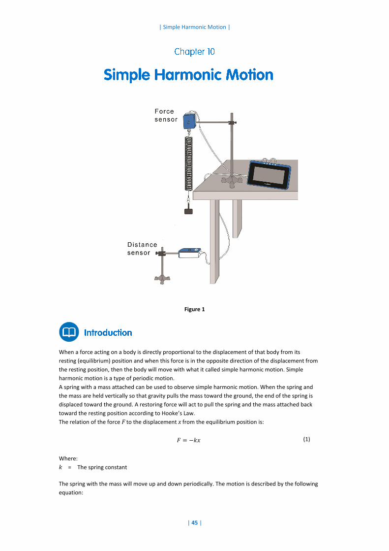
Figure 1
When a force acting on a body is directly proportional to the displacement of that body from its
resting (equilibrium) position and when this force is in the opposite direction of the displacement from
the resting position, then the body will move with what it called simple harmonic motion. Simple
harmonic motion is a type of periodic motion.
A spring with a mass attached can be used to observe simple harmonic motion. When the spring and
the mass are held vertically so that gravity pulls the mass toward the ground, the end of the spring is
displaced toward the ground. A restoring force will act to pull the spring and the mass attached back
toward the resting position according to Hooke’s Law.
The relation of the force F to the displacement x from the equilibrium position is:
𝐹 = −𝑘𝑥 (1)
Where:
k = The spring constant
The spring with the mass will move up and down periodically. The motion is described by the following
equation:
| Simple Harmonic Motion |
| 46 |
𝑥 = 𝐴 cos 2𝜋𝑓𝑡 (2)
Where:
A = The amplitude of the motion
f = The frequency of the motion
The period of the motion is the amount of time it takes to repeat the period of motion once. It is
related to the spring constant and the size of the mass (m, measured in kg):
𝑇 = 2𝜋√𝑚
𝑘 (3)
and can also be expressed as the inverse of the frequency of the motion:
𝑇 =1
𝑓 (4)
In this experiment we examine the motion of a mass attached to a spring and oscillating vertically. The
force acting on the spring and the position of the mass are measured simultaneously.
einstein™Tablet+ with MiLAB or Android/iOS Tablet with MiLAB and einstein™LabMate
Force sensor
Distance sensor
A mass attached to a spring (the frequency of the oscillation should be 0.5-2 Hz and the amplitude
should be 5-20 cm)
1 kg mass (2)
Stand with a clamp to hold the force sensor and the spring
Stand with a clamp to hold the distance sensor
C-clamp to clamp the stand to the counter
Meter stick
1 large 5cm x 8cm index card
Balance to measure the mass
1. Launch MiLAB ( ).
2. Connect the Force sensor to one of the ports on the einstein™Tablet+ or einstein™LabMate.
3. Connect the Distance sensor to one of the ports on the einstein™Tablet+ or einstein™LabMate.
4. Assemble the equipment as shown in Figure 1:
a. Hang the spring from the Force sensor.
b. Carefully attach the 1 kg mass to the spring.
c. Place the Distance sensor directly beneath the mass. When the spring is fully extended, the
mass and the Distance sensor must be at least 40 cm apart.
5. Make sure that only the Force and Distance sensors are selected.
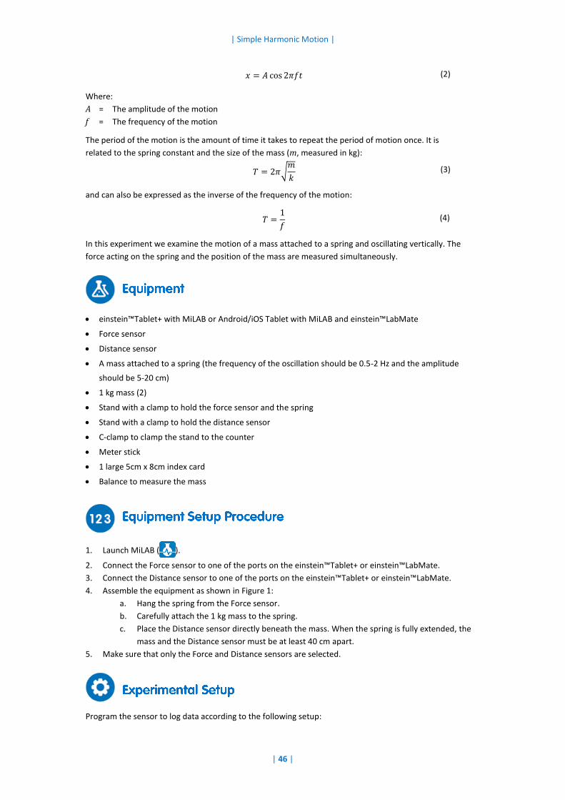
Program the sensor to log data according to the following setup:
| Simple Harmonic Motion |
| 47 |
Force Sensor Force, Pull - positive ( 50 N) (N)
Set As Zero ON
Distance Sensor Distance (m)
Rate: 25/sec
Duration: 40 Sec
1. Using a meter stick and two known masses, measure the spring constant k:
a. Place a 1 kg mass of the end of the spring. Gently let it come to rest. (Do not allow the spring
to oscillate).
b. When the spring comes to its resting (equilibrium) position, use the meter stick to measure
the distance between the floor and the bottom of the 1 kg mass. Record this distance.
c. Put an additional 1 kg mass on the spring and let it come gently to rest. (Do this carefully!)
When the spring comes to its equilibrium position, use the meter stick to measure the
distance between the floor and the bottom of the first 1 kg mass used. Find the difference in
the spring extensions measured.
Note: It is necessary to measure to the bottom of the first 1 kg mass in order to determine the distance the spring stretched. Measurements should always be taken relative to the same point on the first mass.
d. Calculate and record the change in Force, ΔF, using Newton’s second law of motion F = ma.
In the case of using two 1 kg masses, this is given by 1 kg x 9.8 m.s2.
e. Calculate the spring constant k using Hooke’s Law F = kx. Divide the change in force ΔF by
the change in displacement, Δx, of the first 1 kg mass after the second 1 kg mass was added.
2. Using a 1 kg mass, measure the period of oscillation (T) of the mass on the end of the spring:
a. Place the 1 kg mass on the end of the spring, suspended above the Distance sensor.
b. Attach the 5 cm x 8 cm index card to the bottom of the mass so that the broad side of the
card is facing the Distance sensor. Gently pull the 1 kg mass down and let go. It will oscillate
up and down.
3. Tap Run ( ) to begin recording data.
4. After about 15 oscillations, tap Stop ( ).
5. Save your data by tapping Save ( ) on the upper toolbar.
For more information on working with graphs see: Working with Graphs in MiLAB.
1. Working with either the Force curve or the Distance curve, measure the period of oscillation by using
two cursors. Put the first cursor on the first peak and the second cursor on the 11th peak. Record the
value of Δt, which will appear in the text box on the graph as dx. The period, T, will be Δt/10. Record
this value of T.
2. Calculate the spring constant k using the period of oscillation and the following rearrangement of
Equation (3):
𝑘 =4𝜋2𝑚
𝑇2
3. Compare the values of k which you measured using two different methods.
4. Export the data ( ) as a .csv file.
| Simple Harmonic Motion |
| 48 |
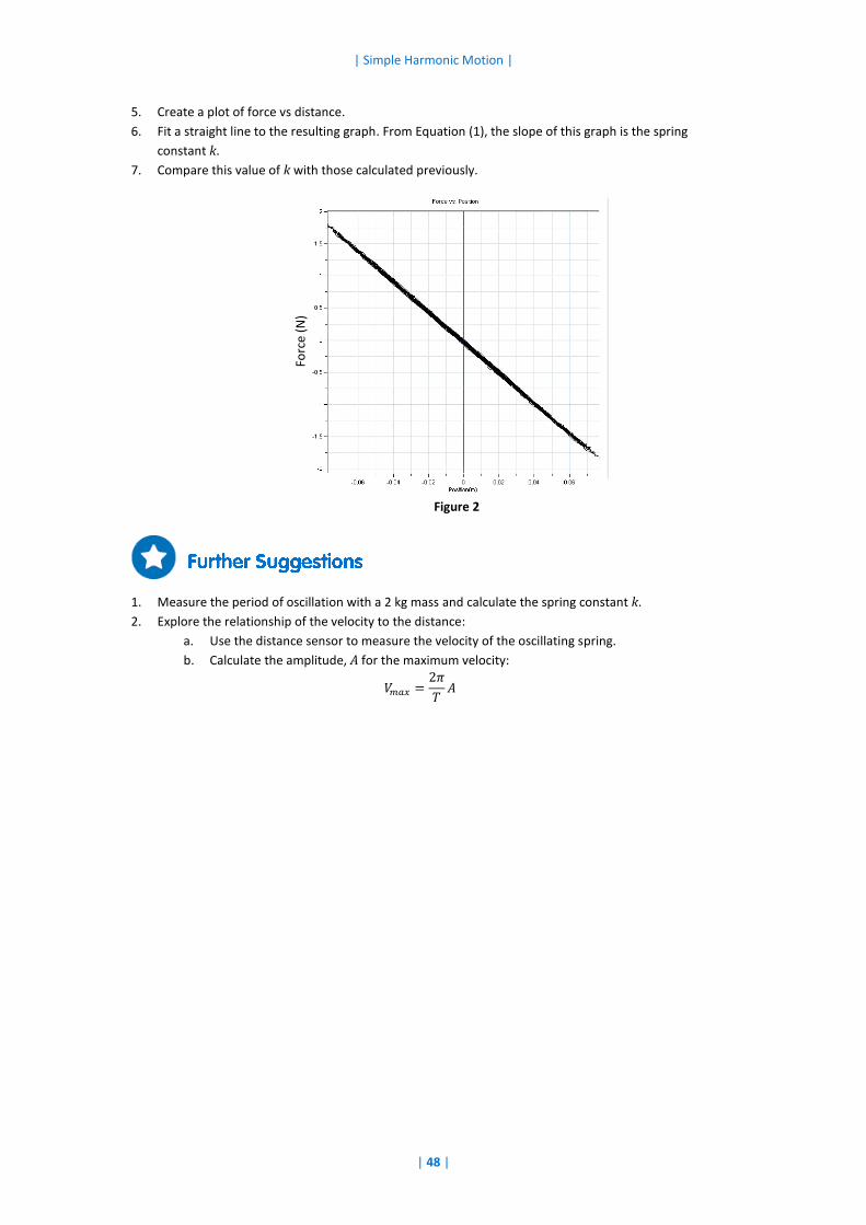
5. Create a plot of force vs distance.
6. Fit a straight line to the resulting graph. From Equation (1), the slope of this graph is the spring
constant k.
7. Compare this value of k with those calculated previously.
Figure 2
1. Measure the period of oscillation with a 2 kg mass and calculate the spring constant k.
2. Explore the relationship of the velocity to the distance:
a. Use the distance sensor to measure the velocity of the oscillating spring.
b. Calculate the amplitude, A for the maximum velocity:
𝑉𝑚𝑎𝑥 =2𝜋
𝑇𝐴
Forc
e (N
)

| Energy in Simple Harmonic Motion |
| 49 |
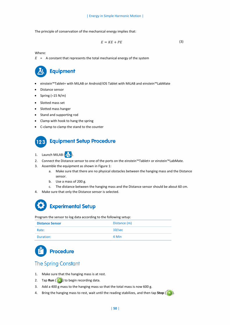
Figure 1
The motion of a mass suspended from a spring is a motion under conservative forces: gravitational
and elastic.
The kinetic energy is given by:
𝐾𝐸 =1
2𝑚𝑣2 (1)
Where:
m = The mass of the suspended body
v = The velocity of the suspended body
The potential energy is given by:
𝑃𝐸 =1
2𝑘𝑥2 (2)
Where:
k = The spring constant
x = The position of the suspended body as measured from the equilibrium point
| Energy in Simple Harmonic Motion |
| 50 |
The principle of conservation of the mechanical energy implies that:
𝐸 = 𝐾𝐸 + 𝑃𝐸 (3)
Where:
E = A constant that represents the total mechanical energy of the system
einstein™Tablet+ with MiLAB or Android/iOS Tablet with MiLAB and einstein™LabMate
Distance sensor
Spring (~15 N/m)
Slotted mass set
Slotted mass hanger
Stand and supporting rod
Clamp with hook to hang the spring
C-clamp to clamp the stand to the counter
1. Launch MiLAB ( ).
2. Connect the Distance sensor to one of the ports on the einstein™Tablet+ or einstein™LabMate.
3. Assemble the equipment as shown in Figure 1:
a. Make sure that there are no physical obstacles between the hanging mass and the Distance
sensor.
b. Use a mass of 200 g.
c. The distance between the hanging mass and the Distance sensor should be about 60 cm.
4. Make sure that only the Distance sensor is selected.
Program the sensor to log data according to the following setup:
Distance Sensor Distance (m)
Rate: 10/sec
Duration: 4 Min
1. Make sure that the hanging mass is at rest.
2. Tap Run ( ) to begin recording data.
3. Add a 400 g mass to the hanging mass so that the total mass is now 600 g.
4. Bring the hanging mass to rest, wait until the reading stabilizes, and then tap Stop ( ).
| Energy in Simple Harmonic Motion |
| 51 |
5. Save your data by tapping Save ( ) on the upper toolbar.
6. Use two cursors to determine how much the spring was stretched after adding the 400 g mass.
7. Calculate k, the spring constant, using Hooke’s Law (F = kx) and the gravitational force on the hanging
mass, m (F = mg):
𝑘 =∆𝑚𝑔
∆𝑙 (4)
Where:
Δl = The displacement of the spring
8. Record this value in your notebook.
1. Make sure that the hanging mass is at rest.
2. Tap Run ( ) to begin recording data.
3. Lift the mass about 5 cm above the equilibrium position and release.
4. After 20 seconds tap Stop ( ).
For more information on working with graphs see: Working with Graphs in MiLAB.
PE k x x
1. Use the cursor to find the equilibrium position of the spring x0. This is the position of the spring before
the oscillations. Record the value of x0 in your notebook.
2. Create a graph of the displacement of the spring (x-x0) as it changes over time with the oscillations:
a. Tap the Function button ( ).
b. Tap the Setup button ( ) next to the Linear function from the Mathematical Functions menu.
c. In the Math Functions window which opens, select the Distance data from the G1 drop down
menu.
d. In the A edit box, enter the negative of the equilibrium position, -x0.
e. Enter Displacement in the Name edit box and m in the Unit edit box.
3. Create a graph of the potential energy as it changes over time with the oscillations:
a. Tap the Function button ( ).
b. Tap the Setup button ( ) next to the Square function from the Mathematical Functions menu.
c. In the Math Functions window which opens, select the displacement data which you calculated
in the previous step from the G1 drop down menu.
d. In the A edit box, enter ½k, that is, half the value of the spring constant.
e. In the B edit box enter 0.
f. Enter PE in the Name edit box and J in the Unit edit box.
g. Hide the Linear function and the Distance graph. The PE graph should be displayed.
KE mv
1. Create a graph of the velocity of the spring, v, as it changes over time with the oscillations:
a. Tap the Function button ( ).
b. Tap the Setup button ( ) next to the Derivative function from the Mathematical Functions

| Energy in Simple Harmonic Motion |
| 52 |
menu.
c. In the Math Functions window which opens, select the Distance data from the G1 drop down
menu.
d. Enter Velocity in the Name edit box and m/s in the Unit edit box.
2. Create a graph of the kinetic energy as it changes over time with the oscillations:
a. Tap the Function button ( ).
b. Tap the Setup button ( ) next to the Square function from the Mathematical Functions
menu.
c. In the Math Functions window which opens, select the calculated velocity data from the G1
drop down menu.
d. In the A edit box, enter half the value of the mass of the weight, m.
e. Type KE in the Name edit box; type J in the Unit edit box.
1. Export the data ( ) as a .csv file.
2. Plot Potential Energy and Kinetic Energy as a function of position.
3. Calculate the total energy (PE+KE) of the system and plot this value on the graph as well.
4. Discuss the graph in terms of the transitions between potential and kinetic energy and conservation of
energy.
| Specific Heat |
| 53 |
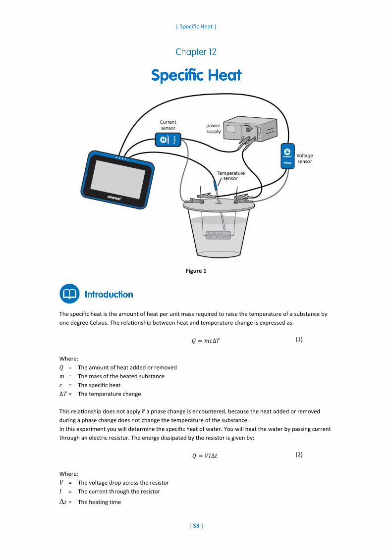
Figure 1
The specific heat is the amount of heat per unit mass required to raise the temperature of a substance by
one degree Celsius. The relationship between heat and temperature change is expressed as:
𝑄 = 𝑚𝑐∆𝑇 (1)
Where:
Q = The amount of heat added or removed
m = The mass of the heated substance
c = The specific heat
ΔT = The temperature change
This relationship does not apply if a phase change is encountered, because the heat added or removed
during a phase change does not change the temperature of the substance.
In this experiment you will determine the specific heat of water. You will heat the water by passing current
through an electric resistor. The energy dissipated by the resistor is given by:
𝑄 = 𝑉𝐼∆𝑡 (2)
Where:
V = The voltage drop across the resistor
I = The current through the resistor
t = The heating time
| Specific Heat |
| 54 |
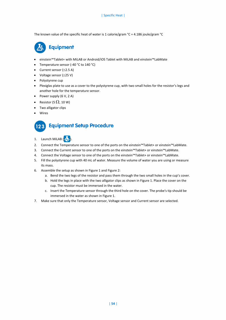
The known value of the specific heat of water is 1 calorie/gram °C = 4.186 joule/gram °C
einstein™Tablet+ with MiLAB or Android/iOS Tablet with MiLAB and einstein™LabMate
Temperature sensor (-40 °C to 140 °C)
Current sensor (2.5 A)
Voltage sensor (25 V)
Polystyrene cup
Plexiglas plate to use as a cover to the polystyrene cup, with two small holes for the resistor’s legs and
another hole for the temperature sensor.
Power supply (6 V, 2 A)
Resistor (5 , 10 W)
Two alligator clips
Wires
1. Launch MiLAB ( ).
2. Connect the Temperature sensor to one of the ports on the einstein™Tablet+ or einstein™LabMate.
3. Connect the Current sensor to one of the ports on the einstein™Tablet+ or einstein™LabMate.
4. Connect the Voltage sensor to one of the ports on the einstein™Tablet+ or einstein™LabMate.
5. Fill the polystyrene cup with 40 mL of water. Measure the volume of water you are using or measure
its mass.
6. Assemble the setup as shown in Figure 1 and Figure 2:
a. Bend the two legs of the resistor and pass them through the two small holes in the cup’s cover.
b. Hold the legs in place with the two alligator clips as shown in Figure 1. Place the cover on the
cup. The resistor must be immersed in the water.
c. Insert the Temperature sensor through the third hole on the cover. The probe's tip should be
immersed in the water as shown in Figure 1.
7. Make sure that only the Temperature sensor, Voltage sensor and Current sensor are selected.
| Specific Heat |
| 55 |
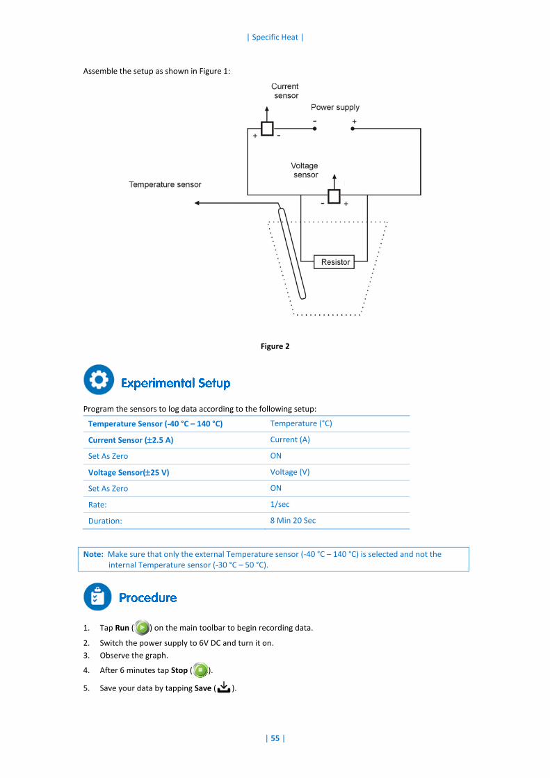
Assemble the setup as shown in Figure 1:
Figure 2
Program the sensors to log data according to the following setup:
Temperature Sensor (-40 °C – 140 °C) Temperature (°C)
Current Sensor (2.5 A) Current (A)
Set As Zero ON
Voltage Sensor(25 V) Voltage (V)
Set As Zero ON
Rate: 1/sec
Duration: 8 Min 20 Sec
Note: Make sure that only the external Temperature sensor (-40 °C – 140 °C) is selected and not the internal Temperature sensor (-30 °C – 50 °C).
1. Tap Run ( ) on the main toolbar to begin recording data.
2. Switch the power supply to 6V DC and turn it on.
3. Observe the graph.
4. After 6 minutes tap Stop ( ).
5. Save your data by tapping Save ( ).
| Specific Heat |
| 56 |
For more information on working with graphs see: Working with Graphs in MiLAB.
1. What is the mass of water in the cup? Record the mass in your notebook and explain how you
determined this number (by measurement or by calculation?).
2. Use the cursor to read the value of the voltage. Record the value in your notebook.
3. Use the cursor to read the value of the current. Record the value in your notebook.
4. Looking at the temperature graph, what can you say about the relationship between the amount of
heat transferred to the water and the temperature change which occurred?
5. Use both cursors to mark two points on the temperature graph. Make sure to select two points in the
region where the temperature is increasing. Record the time difference and the temperature
difference between the two points in your notebook.
6. Use Equation (2) to calculate the amount of heat dissipated by the resistor. Record the value in your
notebook.
7. Use Equation (1) to calculate the specific heat of water. Record the value in your notebook.
8. Compare the value that you have just calculated with the known value (see Introduction).
Repeat the experiment with 80 mL of water and compare the slopes of the two graphs.
| Charge Produced by Friction |
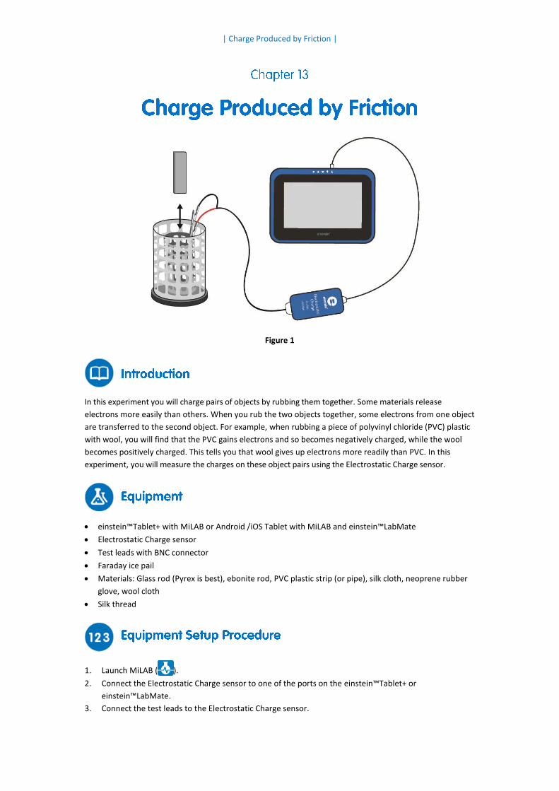
Figure 1
In this experiment you will charge pairs of objects by rubbing them together. Some materials release
electrons more easily than others. When you rub the two objects together, some electrons from one object
are transferred to the second object. For example, when rubbing a piece of polyvinyl chloride (PVC) plastic
with wool, you will find that the PVC gains electrons and so becomes negatively charged, while the wool
becomes positively charged. This tells you that wool gives up electrons more readily than PVC. In this
experiment, you will measure the charges on these object pairs using the Electrostatic Charge sensor.
einstein™Tablet+ with MiLAB or Android /iOS Tablet with MiLAB and einstein™LabMate
Electrostatic Charge sensor
Test leads with BNC connector
Faraday ice pail
Materials: Glass rod (Pyrex is best), ebonite rod, PVC plastic strip (or pipe), silk cloth, neoprene rubber
glove, wool cloth
Silk thread
1. Launch MiLAB ( ).
2. Connect the Electrostatic Charge sensor to one of the ports on the einstein™Tablet+ or
einstein™LabMate.
3. Connect the test leads to the Electrostatic Charge sensor.
| Charge Produced by Friction |
| 58 |
4. Make sure that only the Electrostatic Charge sensor is selected.
Program the sensor to log data according to the following setup:
Electrostatic Charge Sensor Charge, 25 nC (nC)
Set As Zero ON
Rate: 10/sec
Duration: 2 Min
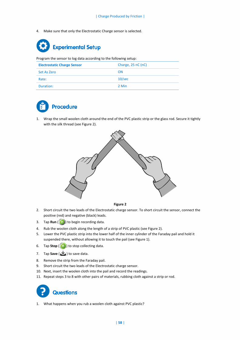
1. Wrap the small woolen cloth around the end of the PVC plastic strip or the glass rod. Secure it tightly
with the silk thread (see Figure 2).
Figure 2
2. Short circuit the two leads of the Electrostatic charge sensor. To short circuit the sensor, connect the
positive (red) and negative (black) leads.
3. Tap Run ( ) to begin recording data.
4. Rub the woolen cloth along the length of a strip of PVC plastic (see Figure 2).
5. Lower the PVC plastic strip into the lower half of the inner cylinder of the Faraday pail and hold it
suspended there, without allowing it to touch the pail (see Figure 1).
6. Tap Stop ( ) to stop collecting data.
7. Tap Save ( ) to save data.
8. Remove the strip from the Faraday pail.
9. Short circuit the two leads of the Electrostatic charge sensor.
10. Next, insert the woolen cloth into the pail and record the readings.
11. Repeat steps 3 to 8 with other pairs of materials, rubbing cloth against a strip or rod.
1. What happens when you rub a woolen cloth against PVC plastic?

| Charge Produced by Friction |
| 59 |
2. Are the objects that have been rubbed together always charged equally and opposite in charge, when
you measure them? Explain.
3. Which of the pairs of materials that you have rubbed together give off electrons more easily?
| Electrification by Contact |
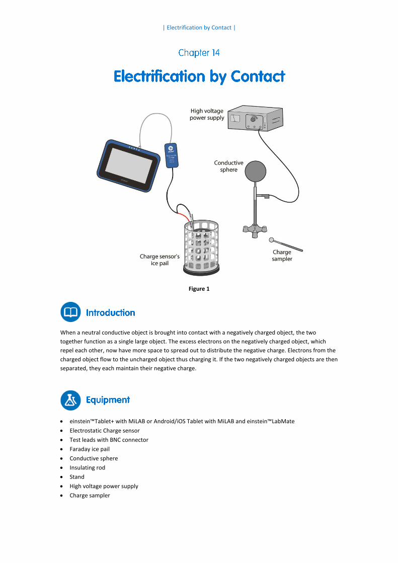
Figure 1
When a neutral conductive object is brought into contact with a negatively charged object, the two
together function as a single large object. The excess electrons on the negatively charged object, which
repel each other, now have more space to spread out to distribute the negative charge. Electrons from the
charged object flow to the uncharged object thus charging it. If the two negatively charged objects are then
separated, they each maintain their negative charge.
einstein™Tablet+ with MiLAB or Android/iOS Tablet with MiLAB and einstein™LabMate
Electrostatic Charge sensor
Test leads with BNC connector
Faraday ice pail
Conductive sphere
Insulating rod
Stand
High voltage power supply
Charge sampler
| Electrification by Contact |
| 61 |
1. Launch MiLAB ( ).
2. Connect the Electrostatic Charge sensor to one of the ports on the einstein™Tablet+ or
einstein™LabMate.
3. Connect the test leads to the Electrostatic Charge sensor.
4. Assemble the equipment as shown in Figure 1.
a. Connect the red lead of the Electrostatic Charge sensor to the inner cylinder of the Faraday
ice pail.
b. Connect the black lead to the outer cylinder of the Faraday ice pail.
c. Connect the conductive sphere to the high voltage output of the high voltage power supply.
5. Make sure that only the Electrostatic Charge sensor is selected.
Note: You may need to ground the outer cylinder of the Faraday ice pail.
Program the sensor to log data according to the following setup:
Electrostatic Charge Sensor Charge, 25 nC (nC)
Set As Zero ON
Rate: 10/sec
Duration: 2 Min
1. Turn on the power supply.
2. Short circuit the two leads of the Electrostatic charge sensor. To short circuit the sensor, connect the
positive (red) and negative (black) leads.
3. Tap Run ( ) to begin recording data.
4. Ground the charge sampler to remove any residual charge from it.
5. Lower the charge sampler into the inner basket of the Faraday ice pail. Observe the resulting graph.
6. Tap Stop ( ) to stop collecting data.
7. Tap Save ( ) to save data.
8. Short circuit the two leads of the Electrostatic charge sensor.
9. Tap Run ( ) to begin recording data.
10. Touch the conductive sphere with the charge sampler, and then lower the charge sampler into the
inner basket of the Faraday ice pail. Observe the resulting graph.
11. Tap Stop ( ) to stop collecting data.
12. Tap Save ( ) to save data.
13. Short circuit the two leads of the Electrostatic charge sensor.
14. Tap Run ( ) to begin recording data.
15. Touch the conductive sphere with the charge sampler a second time, then lower the charge sampler
into the inner basket of the Faraday ice pail. Does the graph change? Explain your observations.
16. Tap Stop ( ) to stop collecting data.

| Electrification by Contact |
| 62 |
17. Tap Save ( ) to save data.
18. Short circuit the two leads of the Electrostatic charge sensor.
19. Tap Run ( ) to begin recording data.
20. Now ground the charge sampler to remove any residual charge from it, then repeat step 7. Explain the
changes in the graph.
21. Tap Stop ( ) to stop collecting data.
22. Tap Save ( ) to save data.
1. Is the conductive sphere charged positively or negatively?
2. Explain how the spheres were charged.
3. Explain the process by which you charged the charge sampler.
| Charge Produced by Induction |
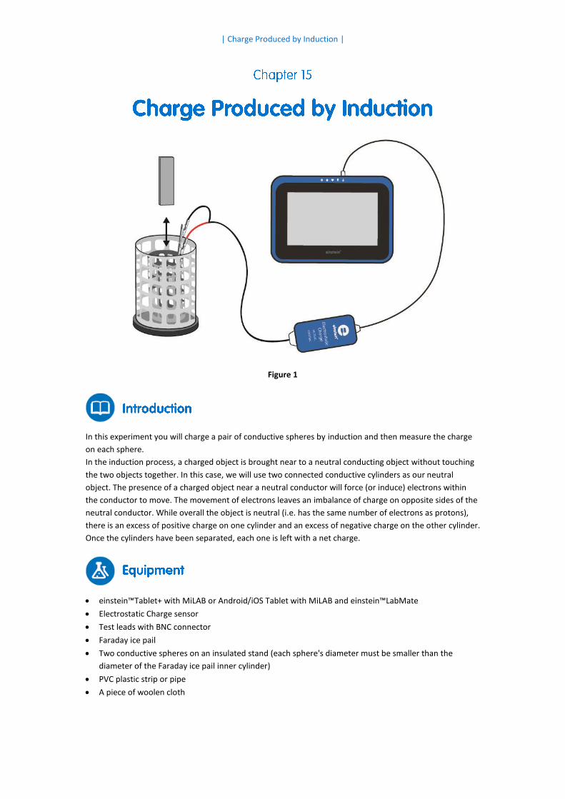
Figure 1
In this experiment you will charge a pair of conductive spheres by induction and then measure the charge
on each sphere.
In the induction process, a charged object is brought near to a neutral conducting object without touching
the two objects together. In this case, we will use two connected conductive cylinders as our neutral
object. The presence of a charged object near a neutral conductor will force (or induce) electrons within
the conductor to move. The movement of electrons leaves an imbalance of charge on opposite sides of the
neutral conductor. While overall the object is neutral (i.e. has the same number of electrons as protons),
there is an excess of positive charge on one cylinder and an excess of negative charge on the other cylinder.
Once the cylinders have been separated, each one is left with a net charge.
einstein™Tablet+ with MiLAB or Android/iOS Tablet with MiLAB and einstein™LabMate
Electrostatic Charge sensor
Test leads with BNC connector
Faraday ice pail
Two conductive spheres on an insulated stand (each sphere's diameter must be smaller than the
diameter of the Faraday ice pail inner cylinder)
PVC plastic strip or pipe
A piece of woolen cloth
| Charge Produced by Induction |
| 64 |
1. Launch MiLAB ( ).
2. Connect the Electrostatic Charge sensor to one of the ports on the einstein™Tablet+ or
einstein™LabMate.
3. Connect the test leads to the Electrostatic Charge sensor.
4. Assemble the equipment as shown in Figure 1.
a. Connect the red lead to the inner cylinder of the Faraday ice pail.
b. Connect the black lead to the outer cylinder of the Faraday ice pail.
5. Make sure that only the Charge sensor is selected.
Note: You may need to ground the outer cylinder of the Faraday ice pail.
Program the sensor to log data according to the following setup:
Electrostatic Charge Sensor Charge, 25 nC (nC)
Set As Zero ON
Rate: 10/sec
Duration: 2 Min
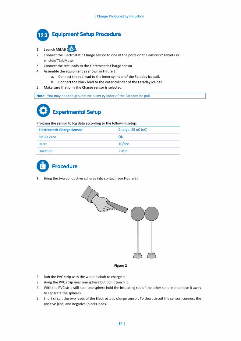
1. Bring the two conductive spheres into contact (see Figure 2).
Figure 2
2. Rub the PVC strip with the woolen cloth to charge it.
3. Bring the PVC strip near one sphere but don’t touch it.
4. With the PVC strip still near one sphere hold the insulating rod of the other sphere and move it away
to separate the spheres.
5. Short circuit the two leads of the Electrostatic charge sensor. To short circuit the sensor, connect the
positive (red) and negative (black) leads.

| Charge Produced by Induction |
| 65 |
6. Tap Run ( ) to begin recording data.
7. Hold the sphere that was nearest to the PVC rod by its insulating rod and insert it into the lower half of
the inner cylinder of the pail, while not letting it touch the pail.
8. Tap Stop ( ) to stop collecting data.
9. Tap Save ( ) to save your data.
10. Remove the sphere.
11. Short circuit the two leads of the Electrostatic charge sensor.
12. Now repeat steps 6 to 10, inserting the other sphere into the pail and recording the readings.
1. What happens when you rub a piece of PVC plastic with a woolen cloth?
2. Explain how the spheres were charged.
3. Were the two spheres charged equally and opposite, when you measured them? Explain.
4. Use your measurements to determine the sign of the charge on the PVC strip. Explain.
| Conductive and Insulating Materials |
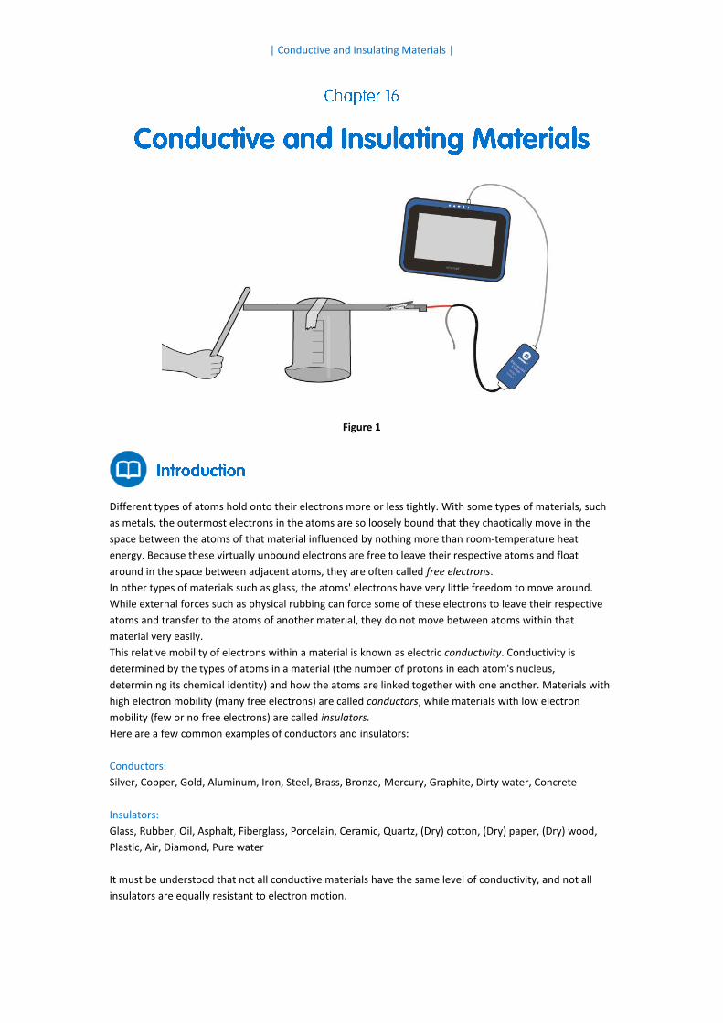
Figure 1
Different types of atoms hold onto their electrons more or less tightly. With some types of materials, such
as metals, the outermost electrons in the atoms are so loosely bound that they chaotically move in the
space between the atoms of that material influenced by nothing more than room-temperature heat
energy. Because these virtually unbound electrons are free to leave their respective atoms and float
around in the space between adjacent atoms, they are often called free electrons.
In other types of materials such as glass, the atoms' electrons have very little freedom to move around.
While external forces such as physical rubbing can force some of these electrons to leave their respective
atoms and transfer to the atoms of another material, they do not move between atoms within that
material very easily.
This relative mobility of electrons within a material is known as electric conductivity. Conductivity is
determined by the types of atoms in a material (the number of protons in each atom's nucleus,
determining its chemical identity) and how the atoms are linked together with one another. Materials with
high electron mobility (many free electrons) are called conductors, while materials with low electron
mobility (few or no free electrons) are called insulators.
Here are a few common examples of conductors and insulators:
Conductors:
Silver, Copper, Gold, Aluminum, Iron, Steel, Brass, Bronze, Mercury, Graphite, Dirty water, Concrete
Insulators:
Glass, Rubber, Oil, Asphalt, Fiberglass, Porcelain, Ceramic, Quartz, (Dry) cotton, (Dry) paper, (Dry) wood,
Plastic, Air, Diamond, Pure water
It must be understood that not all conductive materials have the same level of conductivity, and not all
insulators are equally resistant to electron motion.
| Conductive and Insulating Materials |
| 67 |
For instance, silver is the best conductor in the conductors list, offering easier passage for electrons than
any other material cited. Dirty water and concrete are also listed as conductors, but these materials are
substantially less conductive than any metal.
In this activity we will classify several materials as conductors or insulators by studying the mobility of free
charges in the materials.
einstein™Tablet+ with MiLAB or Android /iOS Tablet with MiLAB and einstein™LabMate
Electrostatic Charge sensor
Test leads with BNC connector
PVC strip or pipe
A piece of woolen cloth
Beaker
Tape
Variety of rods and strips of different materials such as metals, graphite, plastic, wood, paper and
others
1. Launch MiLAB ( ).
2. Connect the Electrostatic Charge sensor to one of the ports on the einstein™Tablet or
einstein™LabMate.
3. Connect the test leads to the Electrostatic Charge sensor.
4. Assemble the equipment as shown in Figure 1.
5. Tape one of your materials on an inverted beaker (see Figure 1).
6. Connect the red lead of the Electrostatic Charge sensor to one end of the material to be tested.
7. Make sure that only the Electrostatic Charge sensor is selected.
Program the sensors to log data according to the following setup:
Electrostatic Charge sensor Charge, 25 nC (nC)
Set As Zero ON
Rate: 10/sec
Duration: 2 Min
1. Short circuit the two leads of the Electrostatic charge sensor. To short circuit the sensor, connect the
positive (red) and negative (black) leads.
2. Tap Run ( ) to begin recording data.
3. Rub the PVC strip with the woolen cloth to charge it.
4. Touch the free end of the test material with the PVC strip.
5. Observe the resulting graph. Will you classify the material as a conductor or as an insulator?

| Conductive and Insulating Materials |
| 68 |
6. Repeat steps 1 to 5 for each material.
Based on your findings, prepare a list of conductive material and a list of insulating materials.
| Voltage Measurements |
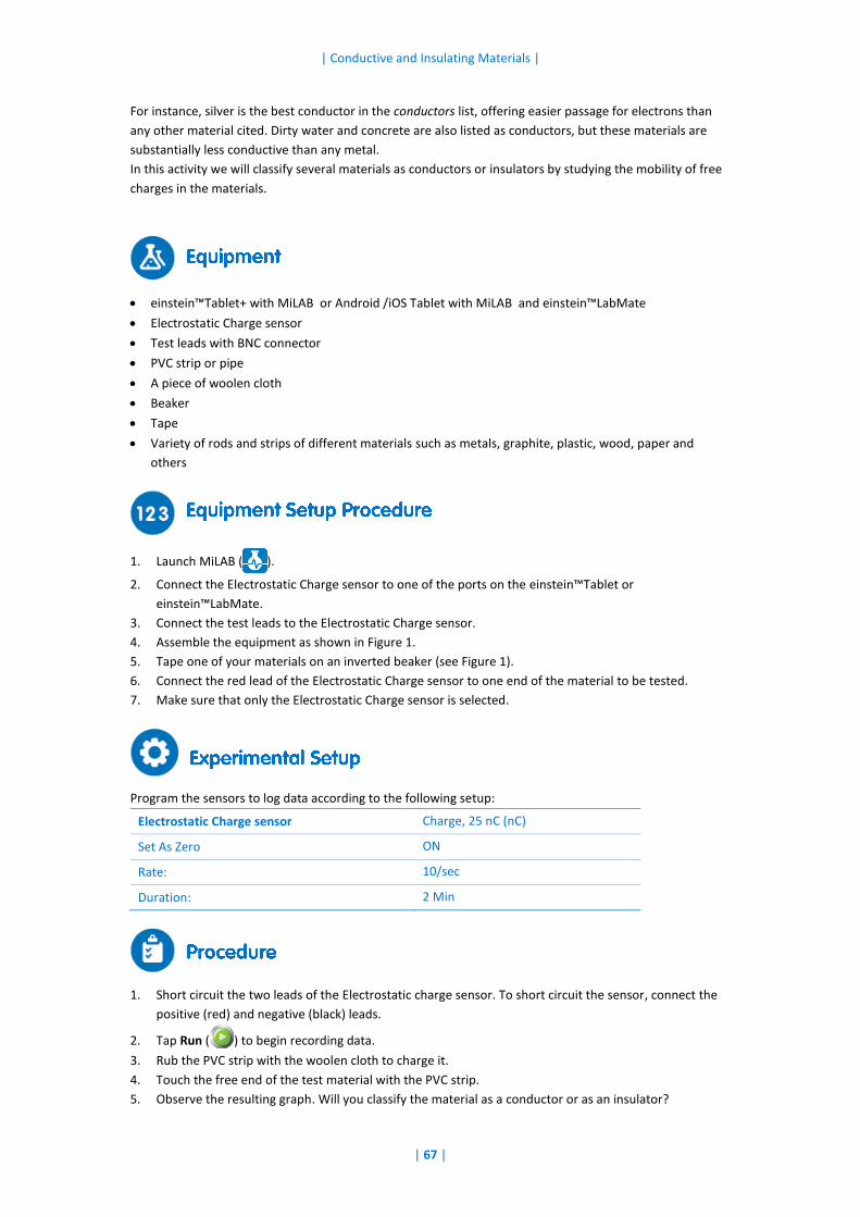
Figure 1
A voltmeter is an instrument used to measure the voltage drop between two points. A digital voltmeter
displays this voltage as a number on a screen. The measuring technique is to digitally compare the
measured voltage drop with an internal reference voltage. The data logger does not just measure the
voltage drop – it also stores the data for future analysis.
In this experiment you will use the voltage sensor to measure voltage drops across several points in a basic
electrical circuit. You will also learn the various display options.
einstein™Tablet+ with MiLAB or Android/iOS Tablet with MiLAB and einstein™LabMate
Voltage sensor (±25 V)
1.5 V battery with battery holder (3)
Small light bulbs, 1.5 V (3)
Light bulb sockets (3)
Connecting wires
Switch (On/Off)
| Voltage Measurements |
| 70 |
1. Launch MiLAB ( ).
2. Connect the Voltage sensor to one of the ports on the einstein™Tablet+ or einstein™LabMate.
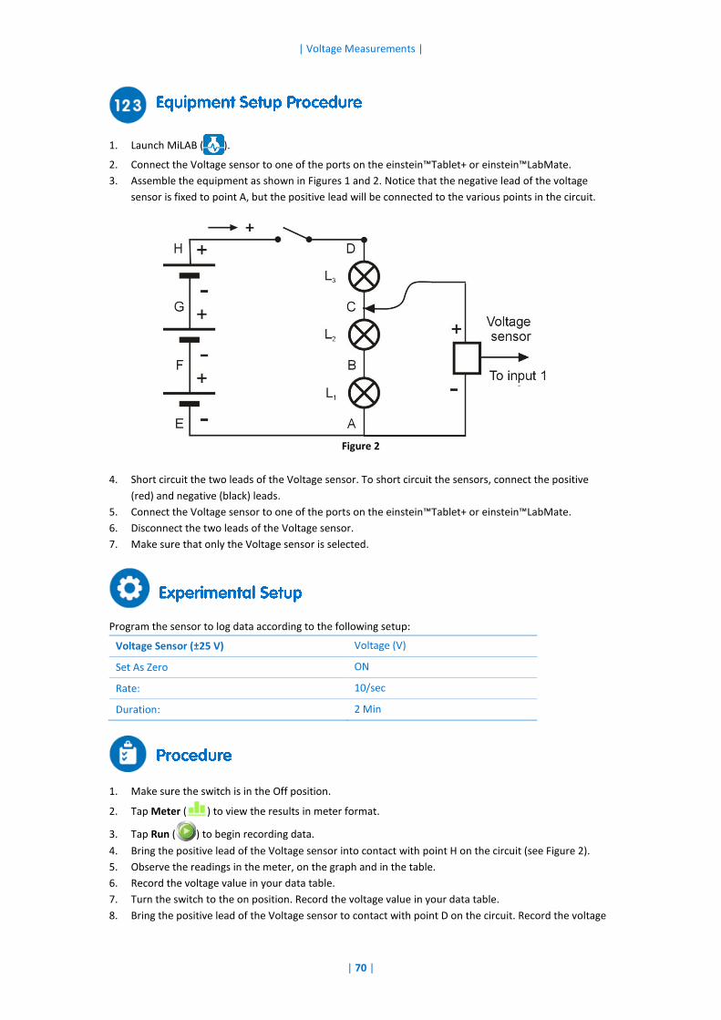
3. Assemble the equipment as shown in Figures 1 and 2. Notice that the negative lead of the voltage
sensor is fixed to point A, but the positive lead will be connected to the various points in the circuit.
Figure 2
4. Short circuit the two leads of the Voltage sensor. To short circuit the sensors, connect the positive
(red) and negative (black) leads.
5. Connect the Voltage sensor to one of the ports on the einstein™Tablet+ or einstein™LabMate.
6. Disconnect the two leads of the Voltage sensor.
7. Make sure that only the Voltage sensor is selected.
Program the sensor to log data according to the following setup:
Voltage Sensor (±25 V) Voltage (V)
Set As Zero ON
Rate: 10/sec
Duration: 2 Min
1. Make sure the switch is in the Off position.
2. Tap Meter ( ) to view the results in meter format.
3. Tap Run ( ) to begin recording data.
4. Bring the positive lead of the Voltage sensor into contact with point H on the circuit (see Figure 2).
5. Observe the readings in the meter, on the graph and in the table.
6. Record the voltage value in your data table.
7. Turn the switch to the on position. Record the voltage value in your data table.
8. Bring the positive lead of the Voltage sensor to contact with point D on the circuit. Record the voltage
| Voltage Measurements |
| 71 |
value in your data table.
9. Repeat step 8 with points C, B, A, E, F and G.
10. The Meters window has four different display options. Explore the Analog ( ), Bar ( ), Color ( )
and Digital ( ) display options.
11. Save your data by tapping Save ( ) on the main toolbar.
Positive lead of the Voltage sensor
connected to point: Voltage Drop (V)
H (switch off)
H (switch on)
D
C
B
A
E
F
G
For more information on working with graphs see: Working with Graphs in MiLAB.
1. Explain the change in the voltage drop between point A and point H after turning the switch from off
to on.
2. Discuss the different measurements that you made.
3. Discuss the advantages of the three different display windows: Meters, Graph and Table and the
different display options within the Meters window.
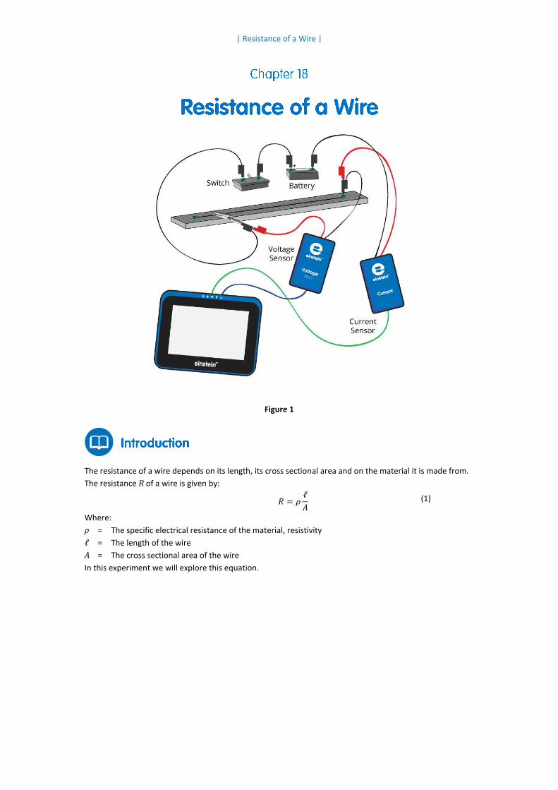
| Resistance of a Wire |
Figure 1
The resistance of a wire depends on its length, its cross sectional area and on the material it is made from.
The resistance R of a wire is given by:
𝑅 = 𝜌ℓ
𝐴 (1)
Where:
ρ = The specific electrical resistance of the material, resistivity
ℓ = The length of the wire
A = The cross sectional area of the wire
In this experiment we will explore this equation.
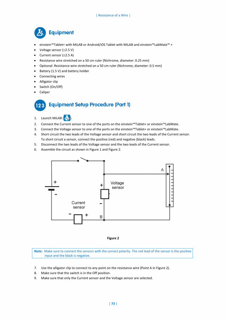
| Resistance of a Wire |
| 73 |
einstein™Tablet+ with MiLAB or Android/iOS Tablet with MiLAB and einstein™LabMate™ +
Voltage sensor (2.5 V)
Current sensor (2.5 A)
Resistance wire stretched on a 50 cm ruler (Nichrome, diameter: 0.25 mm)
Optional: Resistance wire stretched on a 50 cm ruler (Nichrome, diameter: 0.5 mm)
Battery (1.5 V) and battery holder
Connecting wires
Alligator clip
Switch (On/Off)
Caliper
1. Launch MiLAB ( ).
2. Connect the Current sensor to one of the ports on the einstein™Tablet+ or einstein™LabMate.
3. Connect the Voltage sensor to one of the ports on the einstein™Tablet+ or einstein™LabMate.
4. Short circuit the two leads of the Voltage sensor and short circuit the two leads of the Current sensor.
To short circuit a sensor, connect the positive (red) and negative (black) leads.
5. Disconnect the two leads of the Voltage sensor and the two leads of the Current sensor.
6. Assemble the circuit as shown in Figure 1 and Figure 2.
Figure 2
Note: Make sure to connect the sensors with the correct polarity. The red lead of the sensor is the positive input and the black is negative.
7. Use the alligator clip to connect to any point on the resistance wire (Point A in Figure 2).
8. Make sure that the switch is in the Off position.
9. Make sure that only the Current sensor and the Voltage sensor are selected.
| Resistance of a Wire |
| 74 |
Program the sensors to log data according to the following setup:
Voltage Sensor (2.5 V) Voltage (V)
Set As Zero ON
Current Sensor (2.5 A) Current (A)
Set As Zero ON
Rate: 10/sec
Duration: 5 Sec
1. Use the Caliper to measure the diameter of the resistance wire.
2. Clip the alligator clip to the resistance wire next to the 10 cm mark.
3. Tap Meter ( ) to view the results in meter format. Choose the Digital ( ) display option for the
Current and Voltage sensors.
4. Tap Run ( ) to begin recording data. Record the voltage and current values in your data table.
5. Turn the switch to the On position.
6. Tap Run ( ) on the main toolbar each time you wish to record a data sample.
7. Record a data sample.
8. Tap Stop ( ) to stop collecting data.
9. Turn the switch to the Off position.
10. Clip the alligator clip to the resistance wire next to the 15 cm mark and repeat steps 4 to 9.
11. Increase the resistance wire length by measures of 5 cm until reaching 50 cm and repeat steps 4 to 9
for each length.
| Resistance of a Wire |
| 75 |
Diameter of the wire: ________ mm
Cross sectional area of the wire: ________ cm2
For more information on working with graphs see: Working with Graphs in MiLAB.
1. Use Ohm's law (V=IR) and the data from your table to calculate the resistance for every length of wire
in the data table. Record those values in the Resistance column of the table.
2. Plot a graph of the resistance (y-axis) vs. the wire’s length (x-axis).
3. Fit a straight line that passes through the origin to your data points.
4. Does your graph agree with Equation (1)?
5. What are the units of the slope?
6. What is the resistance of the wire per unit length?
7. Use Equation (1) to calculate the specific electrical resistance of the material.
1. Repeat the experiment with a wire of the same material but of a different cross section area.
2. Discuss the dependence of the resistance on the wire’s cross section area.
Length of Wire (cm) Voltage (V) Current (A) Resistance ()
10
15
20
25
30
35
40
45
50
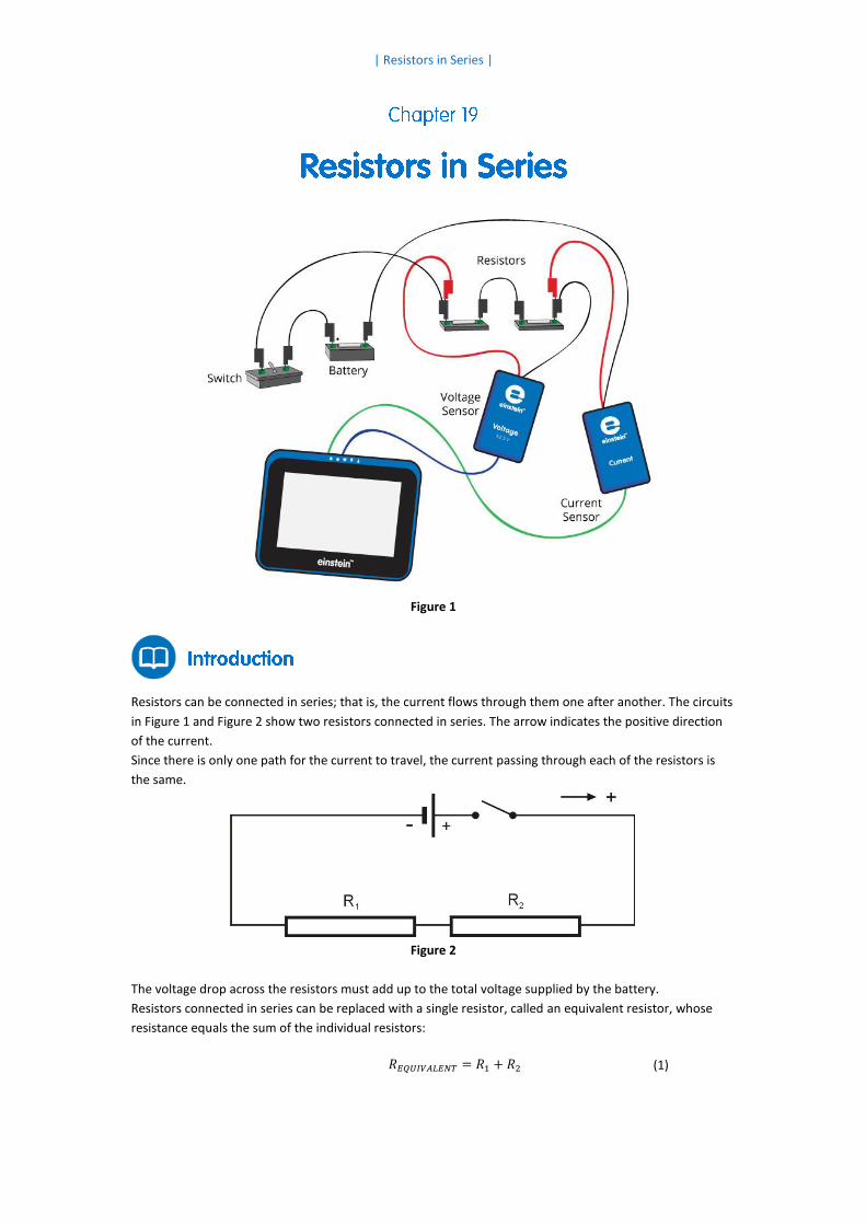
| Resistors in Series |
Figure 1
Resistors can be connected in series; that is, the current flows through them one after another. The circuits
in Figure 1 and Figure 2 show two resistors connected in series. The arrow indicates the positive direction
of the current.
Since there is only one path for the current to travel, the current passing through each of the resistors is
the same.
Figure 2
The voltage drop across the resistors must add up to the total voltage supplied by the battery.
Resistors connected in series can be replaced with a single resistor, called an equivalent resistor, whose
resistance equals the sum of the individual resistors:
𝑅𝐸𝑄𝑈𝐼𝑉𝐴𝐿𝐸𝑁𝑇 = 𝑅1 + 𝑅2 (1)
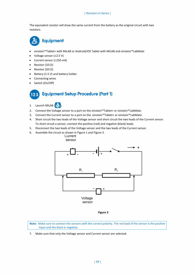
| Resistors in Series |
| 77 |
The equivalent resistor will draw the same current from the battery as the original circuit with two
resistors.
einstein™Tablet+ with MiLAB or Android/iOS Tablet with MiLAB and einstein™LabMate
Voltage sensor (2.5 V)
Current sensor (250 mA)
Resistor (10 )
Resistor (20 )
Battery (1.5 V) and battery holder
Connecting wires
Switch (On/Off)
1. Launch MiLAB ( ).
2. Connect the Voltage sensor to a port on the einstein™Tablet+ or einstein™LabMate.
3. Connect the Current sensor to a port on the einstein™Tablet+ or einstein™LabMate.
4. Short circuit the two leads of the Voltage sensor and short circuit the two leads of the Current sensor.
To short circuit a sensor, connect the positive (red) and negative (black) leads.
5. Disconnect the two leads of the Voltage sensor and the two leads of the Current sensor.
6. Assemble the circuit as shown in Figure 1 and Figure 3.
Figure 3
Note: Make sure to connect the sensors with the correct polarity. The red lead of the sensor is the positive input and the black is negative.
7. Make sure that only the Voltage sensor and Current sensor are selected.
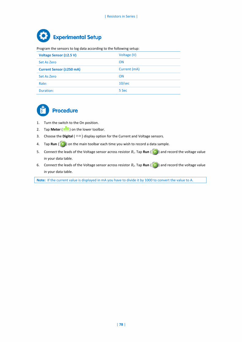
| Resistors in Series |
| 78 |
Program the sensors to log data according to the following setup:
Voltage Sensor (2.5 V) Voltage (V)
Set As Zero ON
Current Sensor (250 mA) Current (mA)
Set As Zero ON
Rate: 10/sec
Duration: 5 Sec
1. Turn the switch to the On position.
2. Tap Meter ( ) on the lower toolbar.
3. Choose the Digital ( ) display option for the Current and Voltage sensors.
4. Tap Run ( ) on the main toolbar each time you wish to record a data sample.
5. Connect the leads of the Voltage sensor across resistor R1. Tap Run ( ) and record the voltage value
in your data table.
6. Connect the leads of the Voltage sensor across resistor R2. Tap Run ( ) and record the voltage value
in your data table.
Note: If the current value is displayed in mA you have to divide it by 1000 to convert the value to A.
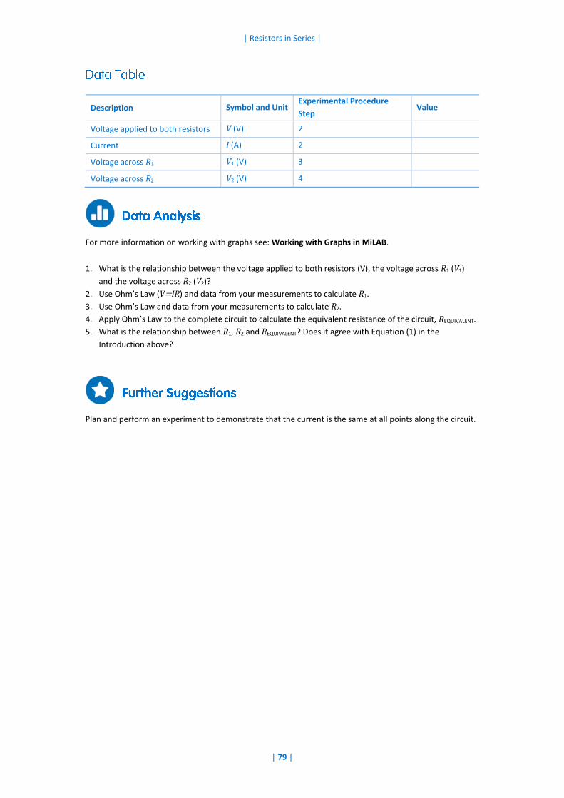
| Resistors in Series |
| 79 |
For more information on working with graphs see: Working with Graphs in MiLAB.
1. What is the relationship between the voltage applied to both resistors (V), the voltage across R1 (V1)
and the voltage across R2 (V2)?
2. Use Ohm’s Law (V=IR) and data from your measurements to calculate R1.
3. Use Ohm’s Law and data from your measurements to calculate R2.
4. Apply Ohm’s Law to the complete circuit to calculate the equivalent resistance of the circuit, REQUIVALENT.
5. What is the relationship between R1, R2 and REQUIVALENT? Does it agree with Equation (1) in the
Introduction above?
Plan and perform an experiment to demonstrate that the current is the same at all points along the circuit.
Description Symbol and Unit Experimental Procedure
Step Value
Voltage applied to both resistors V (V) 2
Current I (A) 2
Voltage across R1 V1 (V) 3
Voltage across R2 V2 (V) 4
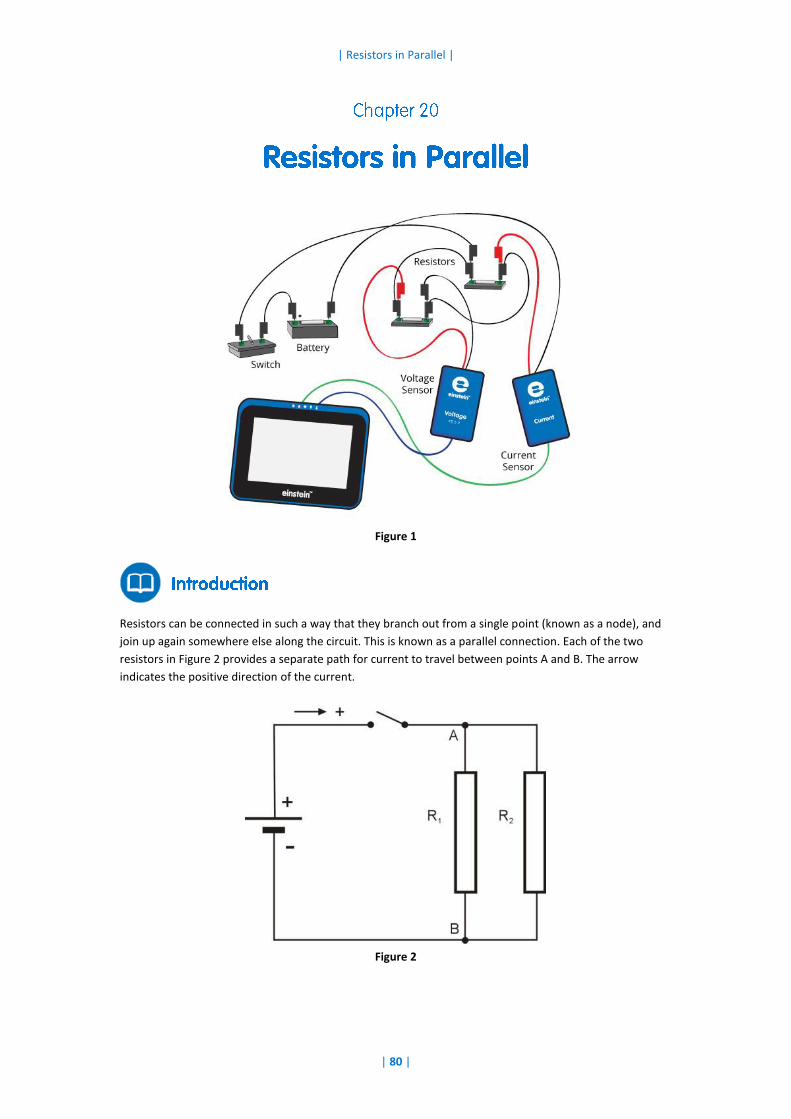
| Resistors in Parallel |
| 80 |
Figure 1
Resistors can be connected in such a way that they branch out from a single point (known as a node), and
join up again somewhere else along the circuit. This is known as a parallel connection. Each of the two
resistors in Figure 2 provides a separate path for current to travel between points A and B. The arrow
indicates the positive direction of the current.
Figure 2
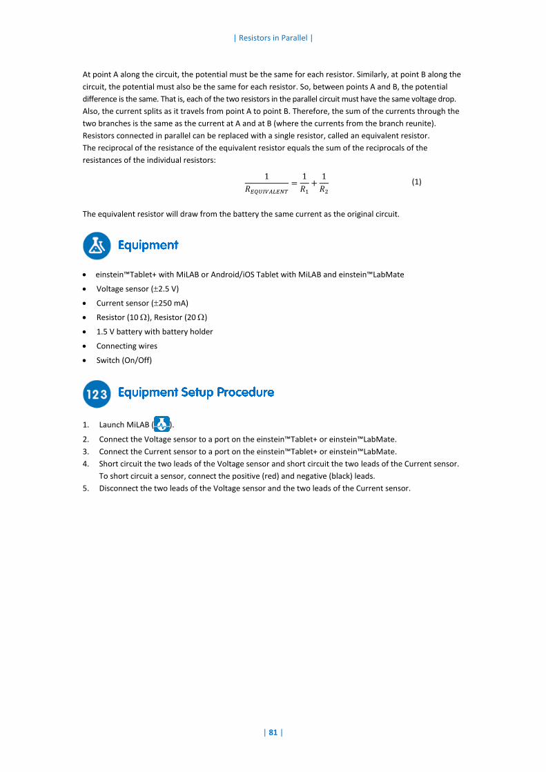
| Resistors in Parallel |
| 81 |
At point A along the circuit, the potential must be the same for each resistor. Similarly, at point B along the
circuit, the potential must also be the same for each resistor. So, between points A and B, the potential
difference is the same. That is, each of the two resistors in the parallel circuit must have the same voltage drop.
Also, the current splits as it travels from point A to point B. Therefore, the sum of the currents through the
two branches is the same as the current at A and at B (where the currents from the branch reunite).
Resistors connected in parallel can be replaced with a single resistor, called an equivalent resistor.
The reciprocal of the resistance of the equivalent resistor equals the sum of the reciprocals of the
resistances of the individual resistors:
1
𝑅𝐸𝑄𝑈𝐼𝑉𝐴𝐿𝐸𝑁𝑇
=1
𝑅1
+1
𝑅2
(1)
The equivalent resistor will draw from the battery the same current as the original circuit.
einstein™Tablet+ with MiLAB or Android/iOS Tablet with MiLAB and einstein™LabMate
Voltage sensor (2.5 V)
Current sensor (250 mA)
Resistor (10 ), Resistor (20 )
1.5 V battery with battery holder
Connecting wires
Switch (On/Off)
1. Launch MiLAB ( ).
2. Connect the Voltage sensor to a port on the einstein™Tablet+ or einstein™LabMate.
3. Connect the Current sensor to a port on the einstein™Tablet+ or einstein™LabMate.
4. Short circuit the two leads of the Voltage sensor and short circuit the two leads of the Current sensor.
To short circuit a sensor, connect the positive (red) and negative (black) leads.
5. Disconnect the two leads of the Voltage sensor and the two leads of the Current sensor.
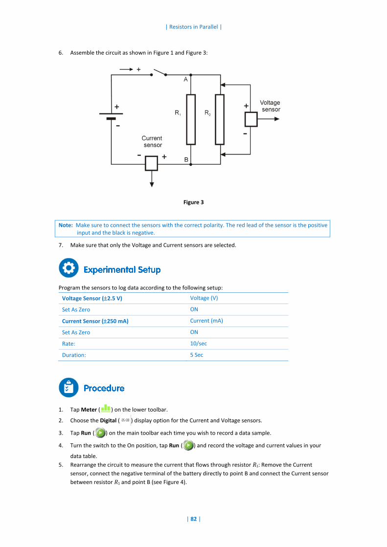
| Resistors in Parallel |
| 82 |
6. Assemble the circuit as shown in Figure 1 and Figure 3:
Figure 3
Note: Make sure to connect the sensors with the correct polarity. The red lead of the sensor is the positive input and the black is negative.
7. Make sure that only the Voltage and Current sensors are selected.
Program the sensors to log data according to the following setup:
Voltage Sensor (2.5 V) Voltage (V)
Set As Zero ON
Current Sensor (250 mA) Current (mA)
Set As Zero ON
Rate: 10/sec
Duration: 5 Sec
1. Tap Meter ( ) on the lower toolbar.
2. Choose the Digital ( ) display option for the Current and Voltage sensors.
3. Tap Run ( ) on the main toolbar each time you wish to record a data sample.
4. Turn the switch to the On position, tap Run ( ) and record the voltage and current values in your
data table.
5. Rearrange the circuit to measure the current that flows through resistor R1: Remove the Current
sensor, connect the negative terminal of the battery directly to point B and connect the Current sensor
between resistor R1 and point B (see Figure 4).
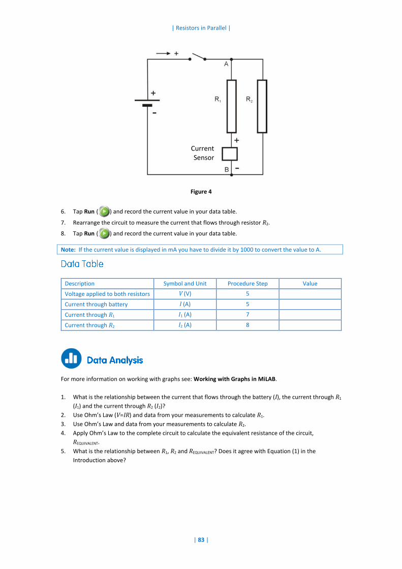
| Resistors in Parallel |
| 83 |
Figure 4
6. Tap Run ( ) and record the current value in your data table.
7. Rearrange the circuit to measure the current that flows through resistor R2.
8. Tap Run ( ) and record the current value in your data table.
Note: If the current value is displayed in mA you have to divide it by 1000 to convert the value to A.
Description Symbol and Unit Procedure Step Value
Voltage applied to both resistors V (V) 5
Current through battery I (A) 5
Current through R1 I1 (A) 7
Current through R2 I2 (A) 8
For more information on working with graphs see: Working with Graphs in MiLAB.
1. What is the relationship between the current that flows through the battery (I), the current through R1
(I1) and the current through R2 (I2)?
2. Use Ohm’s Law (V=IR) and data from your measurements to calculate R1.
3. Use Ohm’s Law and data from your measurements to calculate R2.
4. Apply Ohm’s Law to the complete circuit to calculate the equivalent resistance of the circuit,
REQUIVALENT.
5. What is the relationship between R1, R2 and REQUIVALENT? Does it agree with Equation (1) in the
Introduction above?
Current Sensor
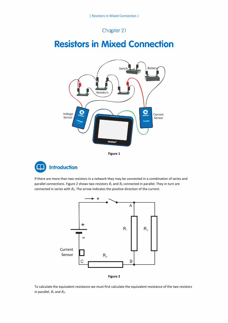
| Resistors in Mixed Connection |
Figure 1
If there are more than two resistors in a network they may be connected in a combination of series and
parallel connections. Figure 2 shows two resistors R1 and R2 connected in parallel. They in turn are
connected in series with R3. The arrow indicates the positive direction of the current.
Figure 2
To calculate the equivalent resistance we must first calculate the equivalent resistance of the two resistors
in parallel, R1 and R2:
Current Sensor
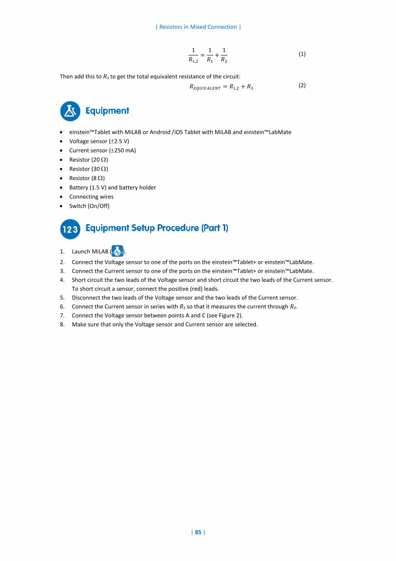
| Resistors in Mixed Connection |
| 85 |
1
𝑅1,2
=1
𝑅1
+1
𝑅2
(1)
Then add this to R3 to get the total equivalent resistance of the circuit:
𝑅𝐸𝑄𝑈𝐼𝑉𝐴𝐿𝐸𝑁𝑇 = 𝑅1,2 + 𝑅3 (2)
einstein™Tablet with MiLAB or Android /iOS Tablet with MiLAB and einstein™LabMate
Voltage sensor (2.5 V)
Current sensor (250 mA)
Resistor (20 )
Resistor (30 )
Resistor (8 )
Battery (1.5 V) and battery holder
Connecting wires
Switch (On/Off)
1. Launch MiLAB ( ).
2. Connect the Voltage sensor to one of the ports on the einstein™Tablet+ or einstein™LabMate.
3. Connect the Current sensor to one of the ports on the einstein™Tablet+ or einstein™LabMate.
4. Short circuit the two leads of the Voltage sensor and short circuit the two leads of the Current sensor.
To short circuit a sensor, connect the positive (red) leads.
5. Disconnect the two leads of the Voltage sensor and the two leads of the Current sensor.
6. Connect the Current sensor in series with R3 so that it measures the current through R3.
7. Connect the Voltage sensor between points A and C (see Figure 2).
8. Make sure that only the Voltage sensor and Current sensor are selected.
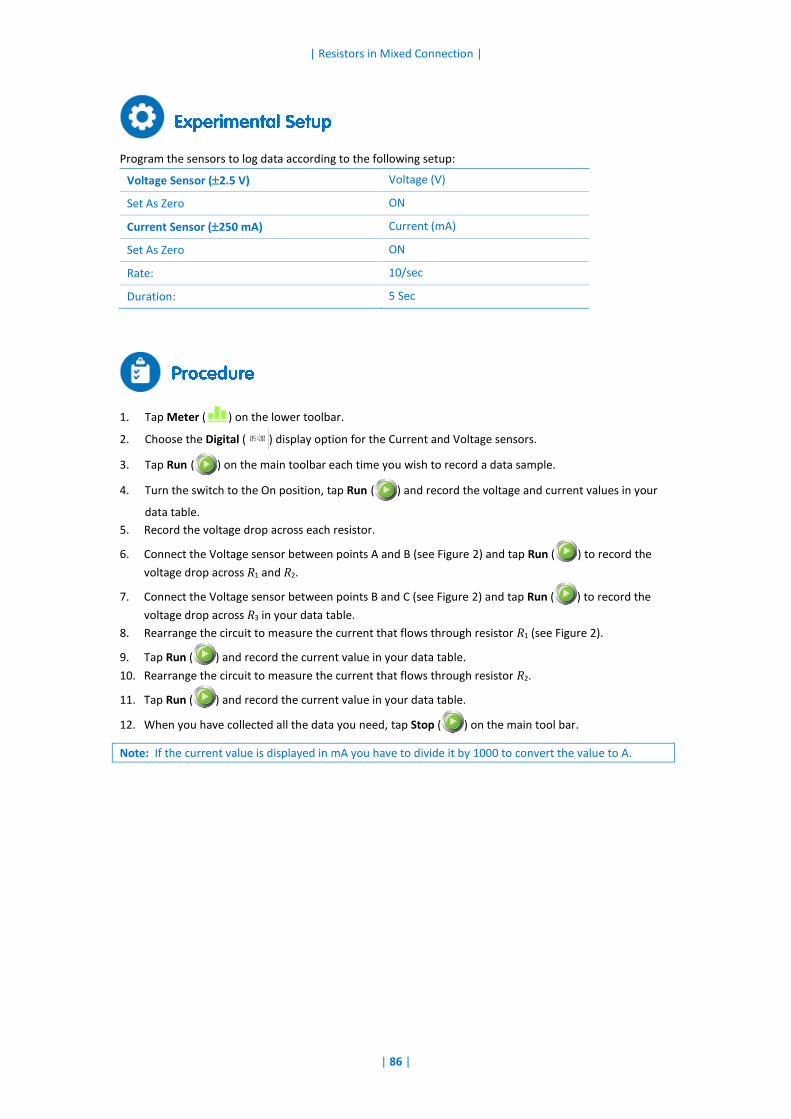
| Resistors in Mixed Connection |
| 86 |
Program the sensors to log data according to the following setup:
Voltage Sensor (2.5 V) Voltage (V)
Set As Zero ON
Current Sensor (250 mA) Current (mA)
Set As Zero ON
Rate: 10/sec
Duration: 5 Sec
1. Tap Meter ( ) on the lower toolbar.
2. Choose the Digital ( ) display option for the Current and Voltage sensors.
3. Tap Run ( ) on the main toolbar each time you wish to record a data sample.
4. Turn the switch to the On position, tap Run ( ) and record the voltage and current values in your
data table.
5. Record the voltage drop across each resistor.
6. Connect the Voltage sensor between points A and B (see Figure 2) and tap Run ( ) to record the
voltage drop across R1 and R2.
7. Connect the Voltage sensor between points B and C (see Figure 2) and tap Run ( ) to record the
voltage drop across R3 in your data table.
8. Rearrange the circuit to measure the current that flows through resistor R1 (see Figure 2).
9. Tap Run ( ) and record the current value in your data table.
10. Rearrange the circuit to measure the current that flows through resistor R2.
11. Tap Run ( ) and record the current value in your data table.
12. When you have collected all the data you need, tap Stop ( ) on the main tool bar.
Note: If the current value is displayed in mA you have to divide it by 1000 to convert the value to A.
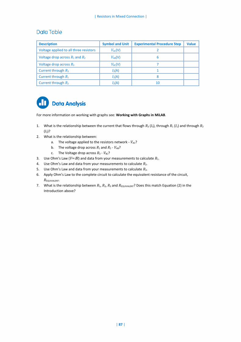
| Resistors in Mixed Connection |
| 87 |
Description Symbol and Unit Experimental Procedure Step Value
Voltage applied to all three resistors VAC(V) 2
Voltage drop across R1 and R2 VAB(V) 6
Voltage drop across R3 VBC(V) 7
Current through R3 I3(A) 1
Current through R1 I1(A) 8
Current through R2 I2(A) 10
For more information on working with graphs see: Working with Graphs in MiLAB.
1. What is the relationship between the current that flows through R3 (I3), through R1 (I1) and through R2
(I2)?
2. What is the relationship between:
a. The voltage applied to the resistors network - VAC?
b. The voltage drop across R1 and R2 - VAB?
c. The Voltage drop across R3 - VBC?
3. Use Ohm’s Law (V=IR) and data from your measurements to calculate R1.
4. Use Ohm’s Law and data from your measurements to calculate R2.
5. Use Ohm’s Law and data from your measurements to calculate R3.
6. Apply Ohm’s Law to the complete circuit to calculate the equivalent resistance of the circuit,
REQUIVALENT.
7. What is the relationship between R1, R2, R3 and REQUIVALENT? Does this match Equation (2) in the
Introduction above?
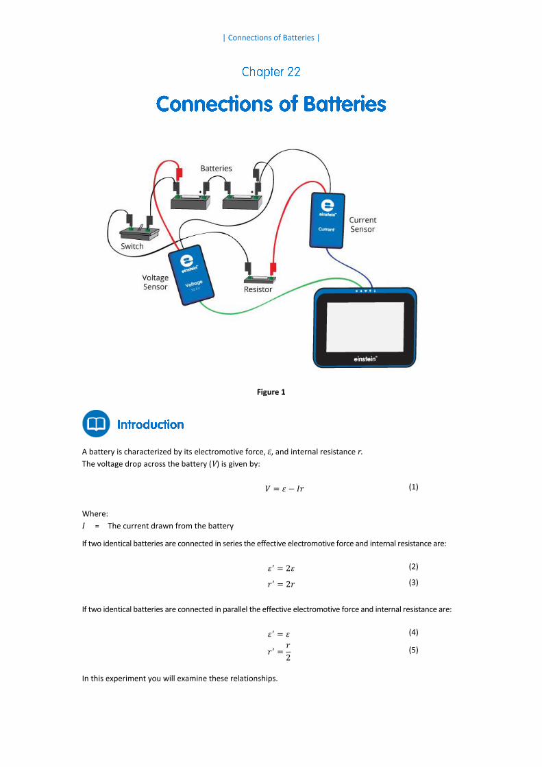
| Connections of Batteries |
Figure 1
A battery is characterized by its electromotive force, Ԑ, and internal resistance r.
The voltage drop across the battery (V) is given by:
𝑉 = 𝜀 − 𝐼𝑟 (1)
Where:
I = The current drawn from the battery
If two identical batteries are connected in series the effective electromotive force and internal resistance are:
𝜀′ = 2𝜀 (2)
𝑟′ = 2𝑟 (3)
If two identical batteries are connected in parallel the effective electromotive force and internal resistance are:
𝜀′ = 𝜀 (4)
𝑟′ =𝑟
2 (5)
In this experiment you will examine these relationships.
| Connections of Batteries |
| 89 |
einstein™Tablet+ with MiLAB or Android/iOS Tablet with MiLAB and einstein™LabMate
Two 1.5 V batteries
Two 1.5 V battery holders
Resistor (2 , 5 W)
Voltage sensor 0 – 5 V
Current sensor 2.5 A
Connecting wires
Switch (On/Off)
1. Launch MiLAB ( ).
2. Connect the Voltage sensor to a port on the einstein™Tablet+ or einstein™LabMate.
3. Connect the Current sensor to a port on the einstein™Tablet+ or einstein™LabMate.
4. Short circuit the two leads of the Voltage sensor and short circuit the two leads of the Current sensor.
To short circuit the sensors, connect the positive (red) leads of the sensor and the negative (black)
leads.
5. Make sure that only the Voltage and Current sensors are selected.
Program the sensors to log data according to the following setup:
Voltage Sensor (2.5 V) Voltage (V)
Set As Zero ON
Current Sensor (2.5 A) Current (A)
Set As Zero ON
Rate: 10/sec
Duration: 5 Sec
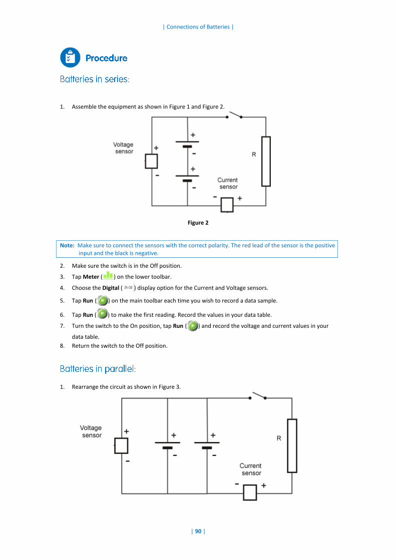
| Connections of Batteries |
| 90 |
1. Assemble the equipment as shown in Figure 1 and Figure 2.
Figure 2
Note: Make sure to connect the sensors with the correct polarity. The red lead of the sensor is the positive input and the black is negative.
2. Make sure the switch is in the Off position.
3. Tap Meter ( ) on the lower toolbar.
4. Choose the Digital ( ) display option for the Current and Voltage sensors.
5. Tap Run ( ) on the main toolbar each time you wish to record a data sample.
6. Tap Run ( ) to make the first reading. Record the values in your data table.
7. Turn the switch to the On position, tap Run ( ) and record the voltage and current values in your
data table.
8. Return the switch to the Off position.
1. Rearrange the circuit as shown in Figure 3.
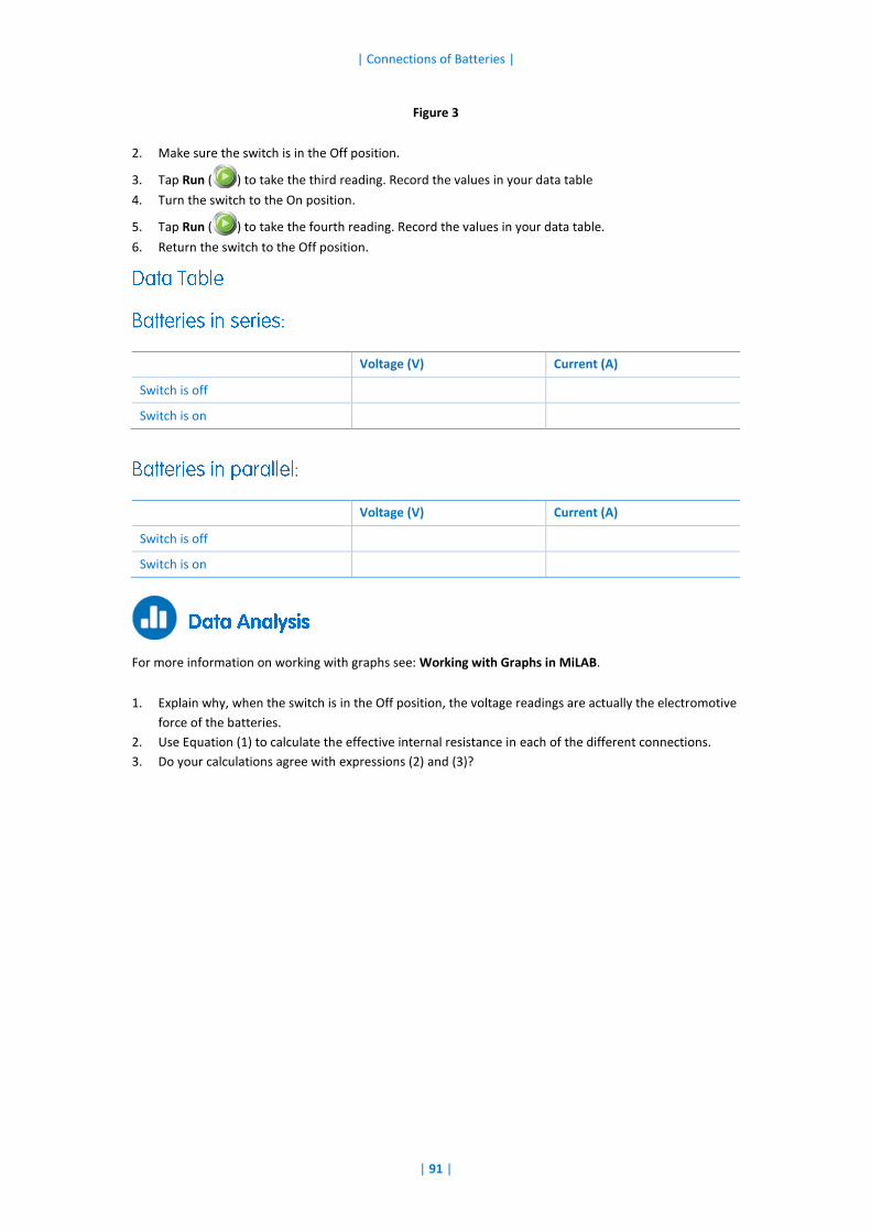
| Connections of Batteries |
| 91 |
Figure 3
2. Make sure the switch is in the Off position.
3. Tap Run ( ) to take the third reading. Record the values in your data table
4. Turn the switch to the On position.
5. Tap Run ( ) to take the fourth reading. Record the values in your data table.
6. Return the switch to the Off position.
For more information on working with graphs see: Working with Graphs in MiLAB.
1. Explain why, when the switch is in the Off position, the voltage readings are actually the electromotive
force of the batteries.
2. Use Equation (1) to calculate the effective internal resistance in each of the different connections.
3. Do your calculations agree with expressions (2) and (3)?
Voltage (V) Current (A)
Switch is off
Switch is on
Voltage (V) Current (A)
Switch is off
Switch is on
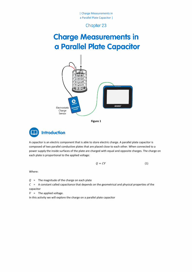
| Charge Measurements in
a Parallel Plate Capacitor |
Figure 1
A capacitor is an electric component that is able to store electric charge. A parallel plate capacitor is
composed of two parallel conductive plates that are placed close to each other. When connected to a
power supply the inside surfaces of the plate are charged with equal and opposite charges. The charge on
each plate is proportional to the applied voltage:
𝑄 = 𝐶𝑉 (1)
Where:
Q = The magnitude of the charge on each plate
C = A constant called capacitance that depends on the geometrical and physical properties of the
capacitor
V = The applied voltage.
In this activity we will explore the charge on a parallel plate capacitor
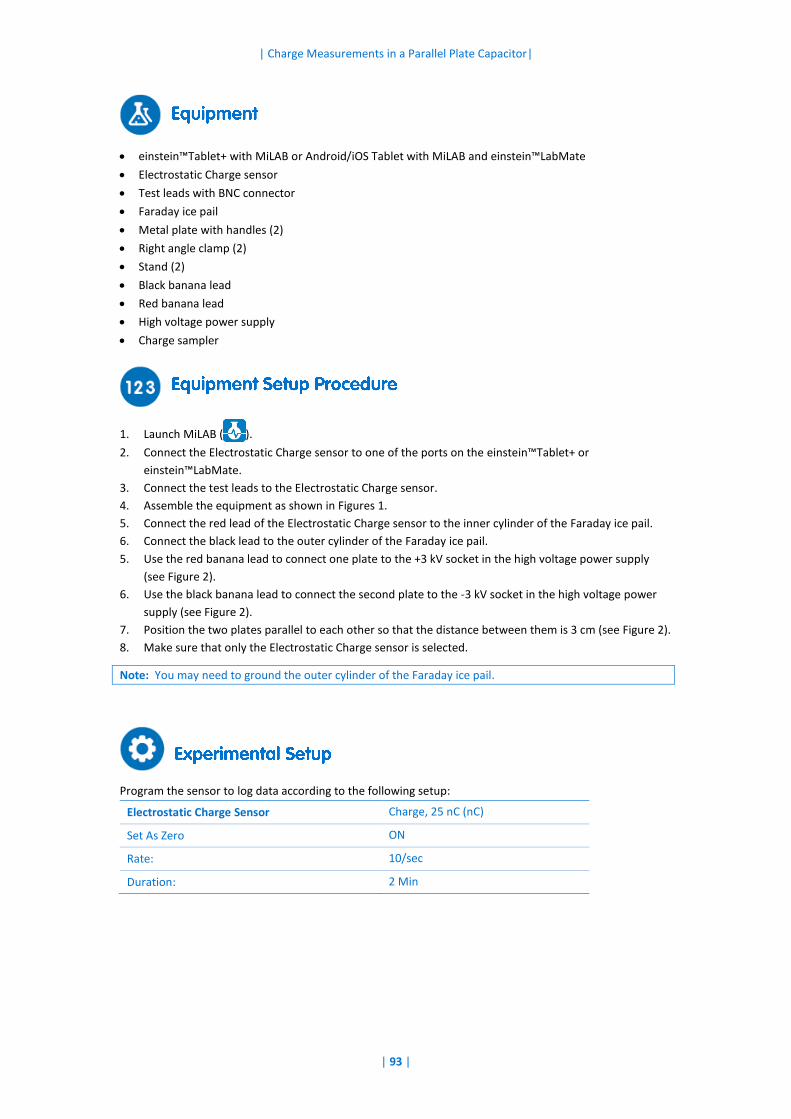
| Charge Measurements in a Parallel Plate Capacitor|
| 93 |
einstein™Tablet+ with MiLAB or Android/iOS Tablet with MiLAB and einstein™LabMate
Electrostatic Charge sensor
Test leads with BNC connector
Faraday ice pail
Metal plate with handles (2)
Right angle clamp (2)
Stand (2)
Black banana lead
Red banana lead
High voltage power supply
Charge sampler
1. Launch MiLAB ( ).
2. Connect the Electrostatic Charge sensor to one of the ports on the einstein™Tablet+ or
einstein™LabMate.
3. Connect the test leads to the Electrostatic Charge sensor.
4. Assemble the equipment as shown in Figures 1.
5. Connect the red lead of the Electrostatic Charge sensor to the inner cylinder of the Faraday ice pail.
6. Connect the black lead to the outer cylinder of the Faraday ice pail.
5. Use the red banana lead to connect one plate to the +3 kV socket in the high voltage power supply
(see Figure 2).
6. Use the black banana lead to connect the second plate to the -3 kV socket in the high voltage power
supply (see Figure 2).
7. Position the two plates parallel to each other so that the distance between them is 3 cm (see Figure 2).
8. Make sure that only the Electrostatic Charge sensor is selected.
Note: You may need to ground the outer cylinder of the Faraday ice pail.
Program the sensor to log data according to the following setup:
Electrostatic Charge Sensor Charge, 25 nC (nC)
Set As Zero ON
Rate: 10/sec
Duration: 2 Min
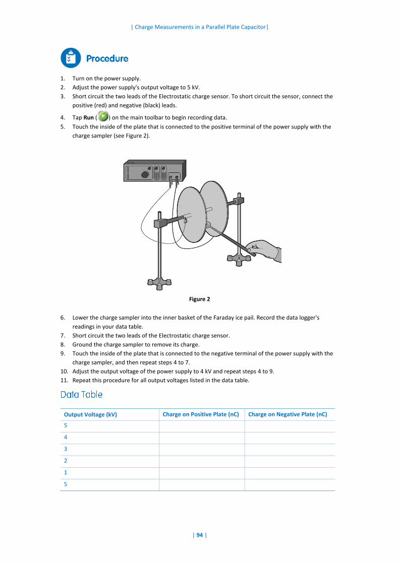
| Charge Measurements in a Parallel Plate Capacitor|
| 94 |
1. Turn on the power supply.
2. Adjust the power supply's output voltage to 5 kV.
3. Short circuit the two leads of the Electrostatic charge sensor. To short circuit the sensor, connect the
positive (red) and negative (black) leads.
4. Tap Run ( ) on the main toolbar to begin recording data.
5. Touch the inside of the plate that is connected to the positive terminal of the power supply with the
charge sampler (see Figure 2).
Figure 2
6. Lower the charge sampler into the inner basket of the Faraday ice pail. Record the data logger's
readings in your data table.
7. Short circuit the two leads of the Electrostatic charge sensor.
8. Ground the charge sampler to remove its charge.
9. Touch the inside of the plate that is connected to the negative terminal of the power supply with the
charge sampler, and then repeat steps 4 to 7.
10. Adjust the output voltage of the power supply to 4 kV and repeat steps 4 to 9.
11. Repeat this procedure for all output voltages listed in the data table.
Output Voltage (kV) Charge on Positive Plate (nC) Charge on Negative Plate (nC)
5
4
3
2
1
5
| Charge Measurements in a Parallel Plate Capacitor|
| 95 |
For more information on working with graphs see: Working with Graphs in MiLAB.
1. Compare the charge on the positive plate to the charge on the negative plate.
2. Create a graph relating the charge measured to the voltage.
3. Discuss the graph in regard to Equation (1).
4. Apply a linear fit to the plot.
5. Use the linear fit equation to calculate the capacitance of the parallel plates.
1. How are the plates charged?
1. Explore the dependence of the capacitance on the distance between the plates. How will your
measurements change if the plates are closer to each other?
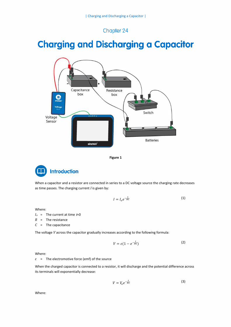
| Charging and Discharging a Capacitor |
Figure 1
When a capacitor and a resistor are connected in series to a DC voltage source the charging rate decreases
as time passes. The charging current I is given by:
𝐼 = 𝐼𝑜𝑒− 𝑡𝑅𝐶 (1)
Where:
Io = The current at time t=0
R = The resistance
C = The capacitance
The voltage V across the capacitor gradually increases according to the following formula:
𝑉 = 𝜀(1 − 𝑒−𝑡
𝑅𝐶) (2)
Where:
ɛ = The electromotive force (emf) of the source
When the charged capacitor is connected to a resistor, it will discharge and the potential difference across
its terminals will exponentially decrease:
𝑉 = 𝑉𝑜𝑒−𝑡
𝑅𝐶 (3)
Where:
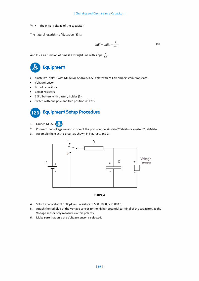
| Charging and Discharging a Capacitor |
| 97 |
V0 = The initial voltage of the capacitor
The natural logarithm of Equation (3) is:
𝑙𝑛𝑉 = 𝑙𝑛𝑉𝑜 −𝑡
𝑅𝐶 (4)
And lnV as a function of time is a straight line with slope 1
𝑅𝐶.
einstein™Tablet+ with MiLAB or Android/iOS Tablet with MiLAB and einstein™LabMate
Voltage sensor
Box of capacitors
Box of resistors
1.5 V battery with battery holder (3)
Switch with one pole and two positions (1P2T)
1. Launch MiLAB ( ).
2. Connect the Voltage sensor to one of the ports on the einstein™Tablet+ or einstein™LabMate.
3. Assemble the electric circuit as shown in Figures 1 and 2:
Figure 2
4. Select a capacitor of 1000F and resistors of 500, 1000 or 2000 .
5. Attach the red plug of the Voltage sensor to the higher potential terminal of the capacitor, as the
Voltage sensor only measures in this polarity.
6. Make sure that only the Voltage sensor is selected.
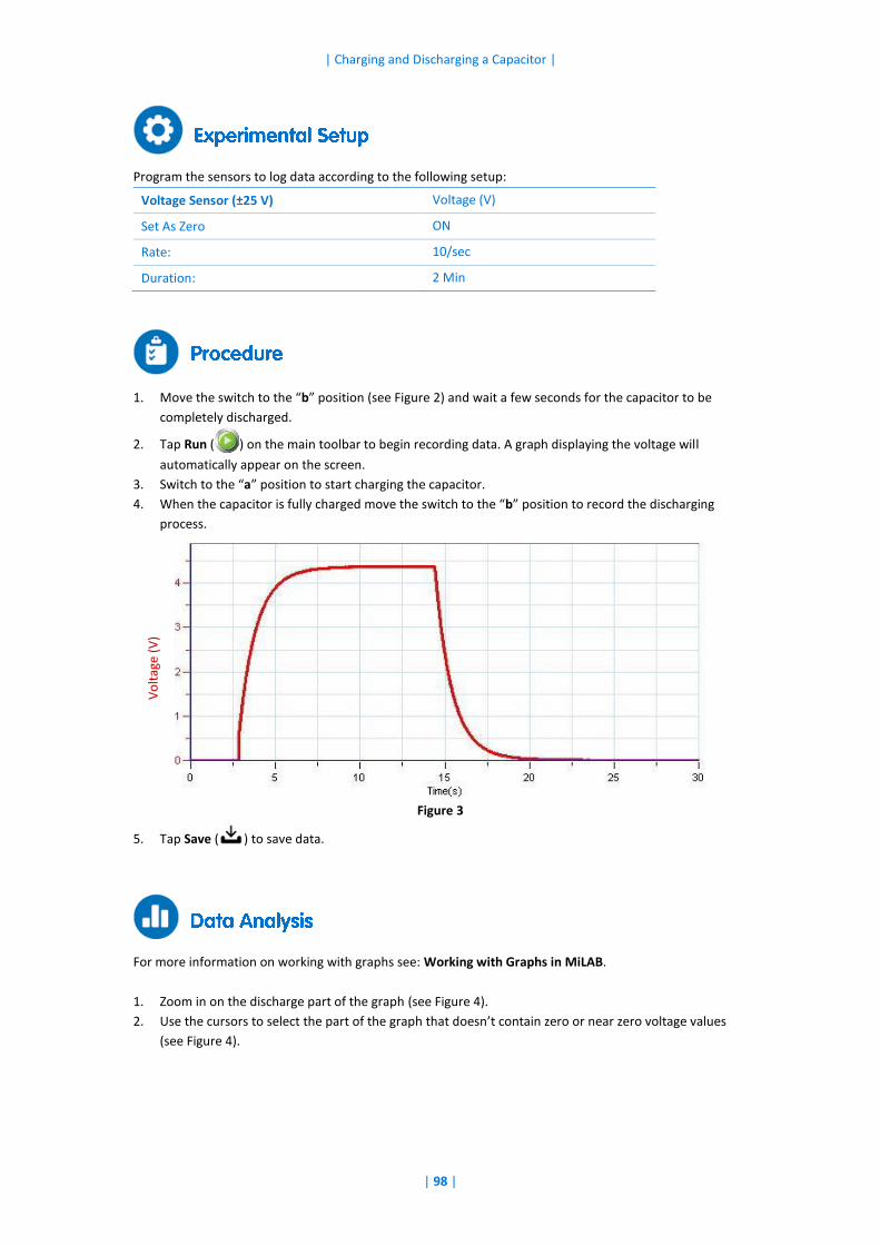
| Charging and Discharging a Capacitor |
| 98 |
Program the sensors to log data according to the following setup:
Voltage Sensor (±25 V) Voltage (V)
Set As Zero ON
Rate: 10/sec
Duration: 2 Min
1. Move the switch to the “b” position (see Figure 2) and wait a few seconds for the capacitor to be
completely discharged.
2. Tap Run ( ) on the main toolbar to begin recording data. A graph displaying the voltage will
automatically appear on the screen.
3. Switch to the “a” position to start charging the capacitor.
4. When the capacitor is fully charged move the switch to the “b” position to record the discharging
process.
Figure 3
5. Tap Save ( ) to save data.
For more information on working with graphs see: Working with Graphs in MiLAB.
1. Zoom in on the discharge part of the graph (see Figure 4).
2. Use the cursors to select the part of the graph that doesn’t contain zero or near zero voltage values
(see Figure 4).
Vo
ltag
e (V
)
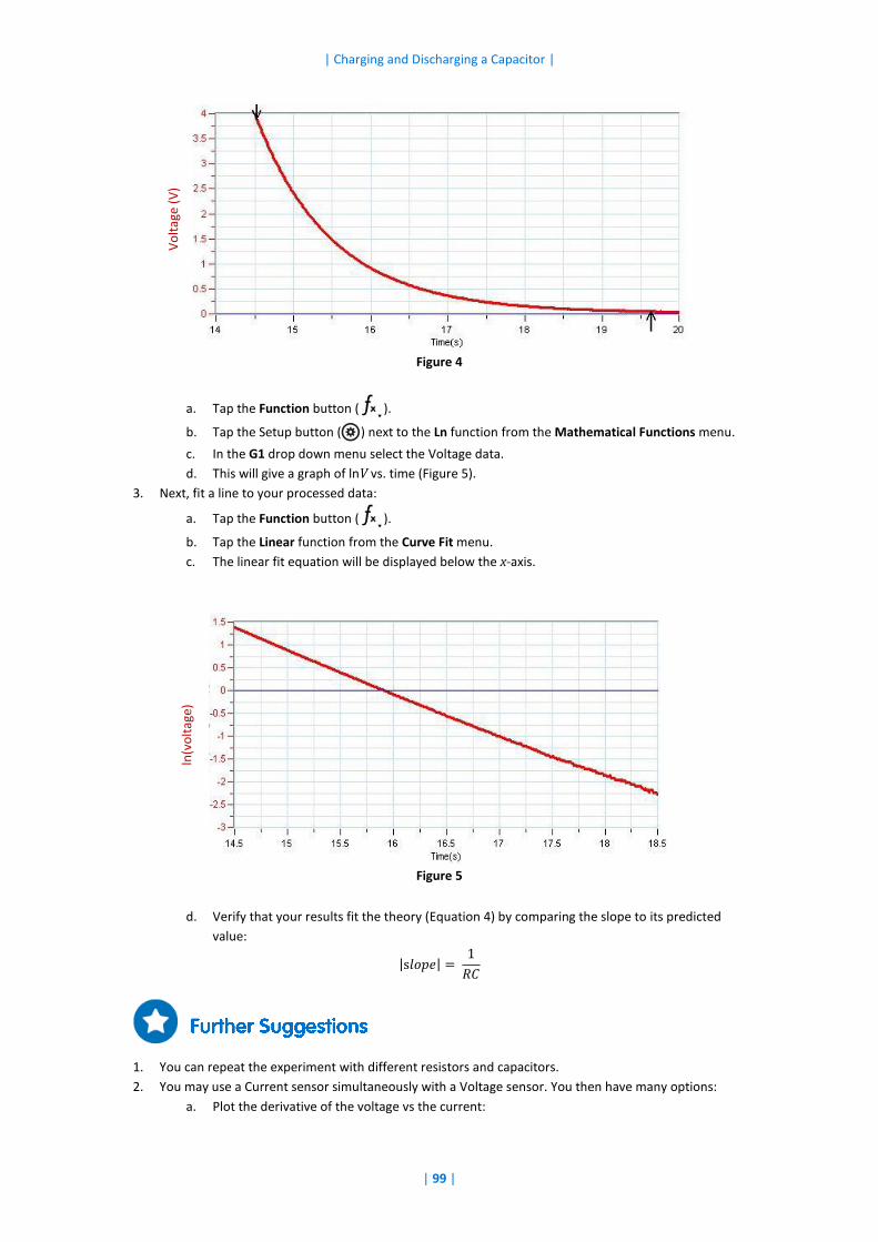
| Charging and Discharging a Capacitor |
| 99 |
Figure 4
a. Tap the Function button ( ).
b. Tap the Setup button ( ) next to the Ln function from the Mathematical Functions menu.
c. In the G1 drop down menu select the Voltage data.
d. This will give a graph of lnV vs. time (Figure 5).
3. Next, fit a line to your processed data:
a. Tap the Function button ( ).
b. Tap the Linear function from the Curve Fit menu.
c. The linear fit equation will be displayed below the x-axis.
Figure 5
d. Verify that your results fit the theory (Equation 4) by comparing the slope to its predicted
value:
|s𝑙𝑜𝑝𝑒| = 1
𝑅𝐶
1. You can repeat the experiment with different resistors and capacitors.
2. You may use a Current sensor simultaneously with a Voltage sensor. You then have many options:
a. Plot the derivative of the voltage vs the current:
Vo
ltag
e (V
) ln
(vo
ltag
e)

| Charging and Discharging a Capacitor |
| 100 |
i. Tap the Function button ( ).
ii. Tap the Setup button ( ) next to the Derivative function from the Mathematical
Functions menu.
iii. In the G1 drop down menu select the Voltage data.
iv. The potential difference between the terminals of the capacitor is proportional to
the charge on them, and since the current is the derivative of the charge it is
expected that the voltage derivative will be proportional to the current.
b. Plot the integral of the current vs the voltage.
i. Tap the Function button ( ).
ii. Tap the Setup button ( ) next to the Integral function from the Mathematical
Functions menu.
iii. In the G1 drop down menu select the current.

| Magnetic Field of a Bar Magnet |
Figure 1
A bar magnet is a seemingly ordinary piece of metal that induces a magnetic field in its vicinity.
This magnetic field affects any magnetic material that lies within it.
In this experiment you will explore the nature of the magnetic field that surrounds a bar magnet.
einstein™Tablet+ with MiLAB or Android /iOS Tablet with MiLAB and einstein™LabMate
Magnetic Field sensor
Bar magnet
Ruler (nonmetallic)
Clear tape
| Magnetic Field of a Bar Magnet |
| 102 |
1. Launch MiLAB ( ).
2. Connect the Magnetic Field sensor sensor to one of the ports on the einstein™Tablet+ or
einstein™LabMate.
3. Set the sensor switch to the low sensitivity range.
4. Tape the ruler to the Tabletop using clear tape.
5. Place the bar magnet parallel to the ruler so that the ruler extends at least 4 cm past the magnet on
either side (see Figure 1). This will enable you to map the magnetic field 4 cm distance from the
magnet.
6. Use the pull down menu in the Sensor Control Panel to select the Magnetic Field sensor.
7. Make sure that only the Magnetic Field sensor is selected.
Program the sensor to log data according to the following setup:
Magnetic Field Sensor Magnetic 10 mT (mT)
Rate: 50/sec
Duration: 5 Sec
1. Position the edge of the magnetic probe on the zero mark of the ruler. Make sure that the probe is
perpendicular to the ruler.
2. Tap Run ( ) each time you wish to record a data sample and record the value in your notebook.
3. Save your data after each measurement by tapping Save ( ) on the main toolbar.
4. Tap Run ( ) on the main toolbar to record the magnetic field’s strength at the 0 cm mark.
5. Now position the edge of the magnetic probe at the 1 cm mark of the ruler, keeping the probe
perpendicular to the ruler, then tap Run ( ) to record the magnetic field’s strength at the 1 cm
mark.
6. Move the sensor along the ruler at 1 cm intervals. Each time take a reading by tapping
Run ( ) until you have reached a point 4 cm beyond the other end of the bar magnet.
| Magnetic Field of a Bar Magnet |
| 103 |
For more information on working with graphs see: Working with Graphs in MiLAB.
Consider the data in your notebook and answer the following questions:
1. What was the strongest positive magnetic field around the bar magnet?
2. Where on the bar magnet did you measure the strongest positive magnetic field?
3. What was the strongest negative magnetic field around the bar magnet?
4. Where on the bar magnet did you measure the strongest negative magnetic field?
5. Where on the bar magnet did you measure zero magnetic field?
6. What can you infer from the fact that the magnetic field around a bar magnet has both positive and
negative values? Will two bar magnets attract or repel each other?
1. Explore the magnetic field of a pair of bar magnets.
2. Explore the magnetic field of a horseshoe (U-shaped) magnet.
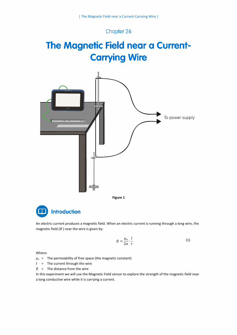
| The Magnetic Field near a Current-Carrying Wire |
Figure 1
An electric current produces a magnetic field. When an electric current is running through a long wire, the
magnetic field (B ) near the wire is given by:
𝐵 =𝜇𝑜
2𝜋∙
𝐼
𝑟 (1)
Where:
μo = The permeability of free space (the magnetic constant)
I = The current through the wire
R = The distance from the wire
In this experiment we will use the Magnetic Field sensor to explore the strength of the magnetic field near
a long conductive wire while it is carrying a current.
| The Magnetic Field near a Current-Carrying Wire |
| 105 |
einstein™Tablet+ with MiLAB or Android/iOS Tablet with MiLAB and einstein™LabMate
Magnetic Field sensor
Long conductive wire (about 2 m long)
10A DC power supply
Stand (2)
Right angle clamp (2)
Short plastic rod (2)
Ruler (nonmetallic)
Clear tape
1. Launch MiLAB ( ).
2. Connect the Magnetic Field sensor to one of the ports on the einstein™Tablet+ or einstein™LabMate.
3. Assemble the equipment as shown in Figure 1.
a. Use the right angle clamps to attach the plastic rods to the stands.
b. Place one stand on the table and the other stand on the floor beneath it.
c. Tape the wire to both the plastic rods. Make sure that the wire is tight and touches the
table’s edge.
d. Tape the ruler to the tabletop with clear tape. Make sure that the zero mark is up against the
wire.
e. Connect the two ends of the wire to the power supply.
f. Set the sensor switch to the high sensitivity range.
4. Use the pull down menu in the Sensor Control Panel to select the Magnetic Field sensor.
5. Make sure that only the Magnetic Field sensor is selected.
Program the sensor to log data according to the following setup:
Magnetic Field Sensor Magnetic 0.2 mT (mT)
Rate: 10/sec
Duration: 5 Sec
1. Position the edge of the magnetic probe on the 1 cm mark of the ruler. Make sure that the probe is
perpendicular to the table edge (see Figure 1).
2. Tap Meter ( ) on the lower toolbar. Use the Digital ( ) display option.
3. Tap Run ( ) on the main toolbar each time you wish to record a data sample.
4. Record the background magnetic field strength at this point by tapping Run ( ). Record the value in
your data table.
5. Turn on the power supply and adjust it to 10 A.
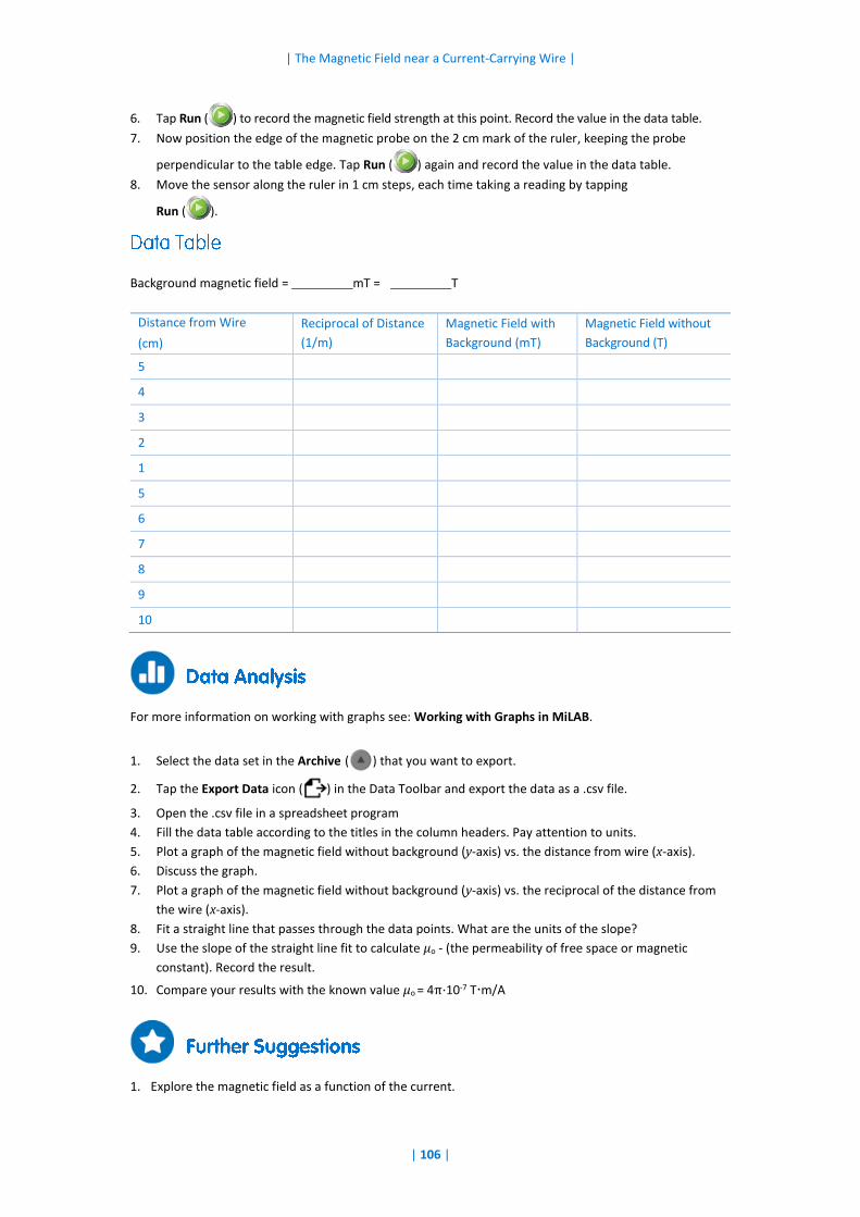
| The Magnetic Field near a Current-Carrying Wire |
| 106 |
6. Tap Run ( ) to record the magnetic field strength at this point. Record the value in the data table.
7. Now position the edge of the magnetic probe on the 2 cm mark of the ruler, keeping the probe
perpendicular to the table edge. Tap Run ( ) again and record the value in the data table.
8. Move the sensor along the ruler in 1 cm steps, each time taking a reading by tapping
Run ( ).
Background magnetic field = ________mT = ________T
For more information on working with graphs see: Working with Graphs in MiLAB.
1. Select the data set in the Archive ( ) that you want to export.
2. Tap the Export Data icon ( ) in the Data Toolbar and export the data as a .csv file.
3. Open the .csv file in a spreadsheet program
4. Fill the data table according to the titles in the column headers. Pay attention to units.
5. Plot a graph of the magnetic field without background (y-axis) vs. the distance from wire (x-axis).
6. Discuss the graph.
7. Plot a graph of the magnetic field without background (y-axis) vs. the reciprocal of the distance from
the wire (x-axis).
8. Fit a straight line that passes through the data points. What are the units of the slope?
9. Use the slope of the straight line fit to calculate μo - (the permeability of free space or magnetic
constant). Record the result.
10. Compare your results with the known value μo = 4π·10-7 T·m/A
1. Explore the magnetic field as a function of the current.
Distance from Wire
(cm)
Reciprocal of Distance
(1/m)
Magnetic Field with
Background (mT)
Magnetic Field without
Background (T)
5
4
3
2
1
5
6
7
8
9
10

| The Magnetic Field near a Current-Carrying Wire |
| 107 |
2. Explore the magnetic field of two parallel long conductive wires carrying current in opposite directions.
3. Explore the magnetic field of two parallel long conductive wires carrying current in the same direction.

| The Magnetic Field of the Earth |
| 108 |
Figure 1
In this experiment we explore the magnetic field of the Earth.
We determine the magnitude and the direction of Earth’s magnetic field, and its inclination.
einstein™Tablet+ with MiLAB or Android/iOS Tablet with MiLAB and einstein™LabMate
Magnetic Field sensor
Compass
Protractor
Plumb (or level)
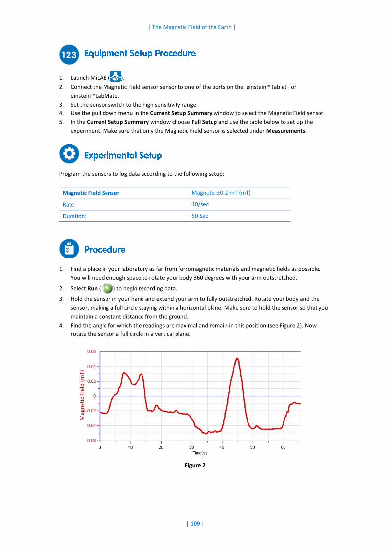
| The Magnetic Field of the Earth |
| 109 |
1. Launch MiLAB ( ).
2. Connect the Magnetic Field sensor sensor to one of the ports on the einstein™Tablet+ or
einstein™LabMate.
3. Set the sensor switch to the high sensitivity range.
4. Use the pull down menu in the Current Setup Summary window to select the Magnetic Field sensor.
5. In the Current Setup Summary window choose Full Setup and use the table below to set up the
experiment. Make sure that only the Magnetic Field sensor is selected under Measurements.
Program the sensors to log data according to the following setup:
Magnetic Field Sensor Magnetic 0.2 mT (mT)
Rate: 10/sec
Duration: 50 Sec
1. Find a place in your laboratory as far from ferromagnetic materials and magnetic fields as possible.
You will need enough space to rotate your body 360 degrees with your arm outstretched.
2. Select Run ( ) to begin recording data.
3. Hold the sensor in your hand and extend your arm to fully outstretched. Rotate your body and the
sensor, making a full circle staying within a horizontal plane. Make sure to hold the sensor so that you
maintain a constant distance from the ground.
4. Find the angle for which the readings are maximal and remain in this position (see Figure 2). Now
rotate the sensor a full circle in a vertical plane.
Figure 2
Mag
net
ic F
ield
(m
T)
| The Magnetic Field of the Earth |
| 110 |
For more information on working with graphs see: Working with Graphs in MiLAB.
1. Zoom in on the data acquired during the vertical circling.
2. Use two cursors to select the maximum and minimum in this part of the graph. The difference
between these points will be now displayed in the information bar below the graph window. That
should be twice the magnitude of the vertical component of the magnetic field of the Earth.
3. Write this value down in your notebook.
4. Zoom in on the data acquired during the horizontal circling.
5. Use two cursors to select the maximum and minimum in this part of the graph. This difference
between theses points will be now displayed in the information bar below the graph window. That
should be twice the magnitude of the horizontal component of the magnetic field of the Earth.
6. Write this value down in your notebook.
7. Use these two results to find the angle of inclination of the magnetic field of the Earth.
8. Write the angle down in your notebook.
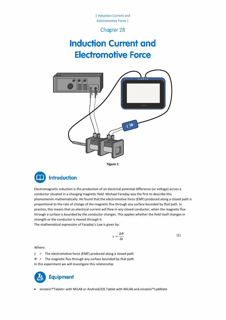
| Induction Current and
Electromotive Force |
Figure 1
Electromagnetic induction is the production of an electrical potential difference (or voltage) across a
conductor situated in a changing magnetic field. Michael Faraday was the first to describe this
phenomenon mathematically. He found that the electromotive force (EMF) produced along a closed path is
proportional to the rate of change of the magnetic flux through any surface bounded by that path. In
practice, this means that an electrical current will flow in any closed conductor, when the magnetic flux
through a surface is bounded by the conductor changes. This applies whether the field itself changes in
strength or the conductor is moved through it.
The mathematical expression of Faraday’s Law is given by:
𝜀 =∆𝛷
∆𝑡 (1)
Where:
Ɛ = The electromotive force (EMF) produced along a closed path
Φ = The magnetic flux through any surface bounded by that path
In this experiment we will investigate this relationship
einstein™Tablet+ with MiLAB or Android/iOS Tablet with MiLAB and einstein™LabMate
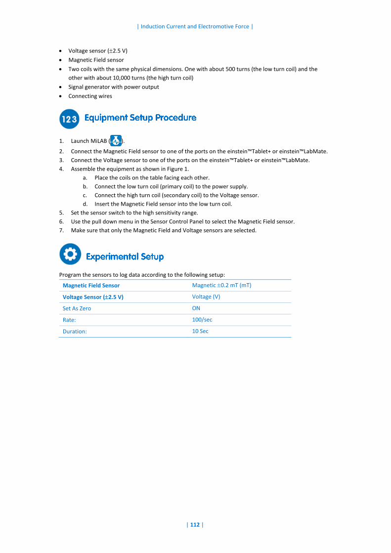
| Induction Current and Electromotive Force |
| 112 |
Voltage sensor (2.5 V)
Magnetic Field sensor
Two coils with the same physical dimensions. One with about 500 turns (the low turn coil) and the
other with about 10,000 turns (the high turn coil)
Signal generator with power output
Connecting wires
1. Launch MiLAB ( ).
2. Connect the Magnetic Field sensor to one of the ports on the einstein™Tablet+ or einstein™LabMate.
3. Connect the Voltage sensor to one of the ports on the einstein™Tablet+ or einstein™LabMate.
4. Assemble the equipment as shown in Figure 1.
a. Place the coils on the table facing each other.
b. Connect the low turn coil (primary coil) to the power supply.
c. Connect the high turn coil (secondary coil) to the Voltage sensor.
d. Insert the Magnetic Field sensor into the low turn coil.
5. Set the sensor switch to the high sensitivity range.
6. Use the pull down menu in the Sensor Control Panel to select the Magnetic Field sensor.
7. Make sure that only the Magnetic Field and Voltage sensors are selected.
Program the sensors to log data according to the following setup:
Magnetic Field Sensor Magnetic 0.2 mT (mT)
Voltage Sensor (2.5 V) Voltage (V)
Set As Zero ON
Rate: 100/sec
Duration: 10 Sec

| Induction Current and Electromotive Force |
| 113 |
1. Turn on the signal generator.
2. Adjust the signal generator to a frequency of 1 Hz and triangular waveform.
3. Tap Run ( ) to begin recording data.
4. Wait for 20 seconds then tap Stop ( ).
5. Save your data by tapping Save ( ).
6. Change the signal generator’s frequency to 2 Hz and repeat steps 3 to 5.
7. Return to a frequency of 1Hz and change the signal generator’s waveform to sinusoidal,
then repeat steps 3 to 6.
For more information on working with graphs see: Working with Graphs in MiLAB.
1. Select Archive ( ) and then select and display the first graph you produced.
2. Discuss the graph in view of Faraday’s Induction Law (Equation (1)).
3. Select Archive ( ) and then select and display the second graph you produced.
4. Discuss the graph in view of Faraday’s Induction Law. What was the effect of doubling the frequency?
5. Select Archive ( ) and then select and display the third graph you produced.
6. Discuss the graph in view of Faraday’s Induction Law. Does the induced voltage graph fit the
derivative of the magnetic field function?
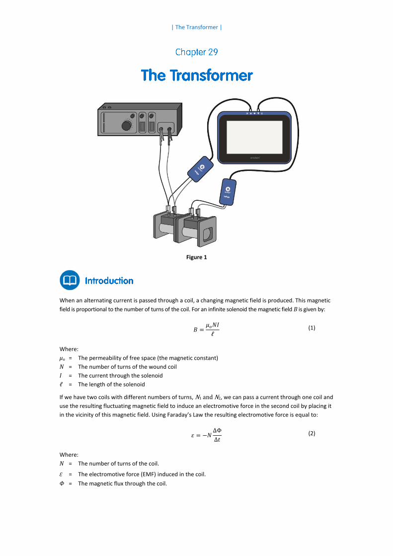
| The Transformer |
Figure 1
When an alternating current is passed through a coil, a changing magnetic field is produced. This magnetic
field is proportional to the number of turns of the coil. For an infinite solenoid the magnetic field B is given by:
𝐵 =𝜇𝑜𝑁𝐼
ℓ (1)
Where:
μo = The permeability of free space (the magnetic constant)
N = The number of turns of the wound coil
I = The current through the solenoid
ℓ = The length of the solenoid
If we have two coils with different numbers of turns, N1 and N2, we can pass a current through one coil and
use the resulting fluctuating magnetic field to induce an electromotive force in the second coil by placing it
in the vicinity of this magnetic field. Using Faraday’s Law the resulting electromotive force is equal to:
𝜀 = −𝑁∆Φ
∆𝑡 (2)
Where:
N = The number of turns of the coil.
Ɛ = The electromotive force (EMF) induced in the coil. Φ = The magnetic flux through the coil.
| The Transformer |
| 115 |
Assuming that all the magnetic flux created by the first (primary) coil flows through the second (secondary)
coil we get the transformer equation:
𝜀1
𝜀2
=𝑁1
𝑁2
(3)
Where Ɛ1 and N1 are the electromotive force and number of turns of the primary coil, through which the
current is passed. Ɛ2 and N2 are the electromotive force and number of turns of the secondary coil, in
which the electromotive force is induced.
In this activity we will investigate Equation (3).
einstein™Tablet + with MiLAB or Android/iOS Tablet with MiLAB and einstein™LabMate
Voltage sensor (±25 V)
Voltage sensor (±2.5 V)
Signal generator
Power supply
Coil (400 turns)
Coil (1600 turns)
Armature
U core with armature
Banana cords (2)
1. Launch MiLAB ( ).
2. Connect the ±2.5 Voltage sensor to one of the ports on the einstein™Tablet+ or einstein™LabMate
then connect the banana plugs to the 400 turns coil (primary coil)..
3. Connect the ±25 Voltage sensor to one of the ports on the einstein™Tablet+ or einstein™LabMate
then connect the banana plugs to the 1600 turns coil (secondary coil).
4. Assemble the equipment as shown in Figure 1.
a. Use the banana cords to connect the 400 turns coil (primary coil) to the power output of the
signal generator.
b. Place the 1600 turns coil (secondary coil) next to the primary coil.
5. Make sure that only the two Voltage sensors are selected.
Program the sensors to log data according to the following setup:
Voltage Sensor (2.5 V) Voltage (V)
Set As Zero ON
Voltage Sensor (25 V) Voltage (V)
Set As Zero ON
Rate: 100/sec
Duration: 20 Sec
| The Transformer |
| 116 |
1. Turn on the signal generator and set it to:
Output voltage: ~2 V
Frequency: 5 Hz
Waveform: Sinusoidal
2. Tap Run ( ) on the main toolbar to begin recording data.
3. After a couple of seconds tap Stop ( ).
4. Save your data by tapping Save ( ).
5. Use the cursors to measure the voltage drops across the primary and secondary coils. Record the
values in your notebook.
6. Insert the armature into both the coils and repeat steps 2 to 5.
7. Mount the coils on the U core and close it with the armature and repeat the experiment..
8. Repeat steps 2 to 5.
9. Set the signal generator's frequency to 50 Hz and increase the data logger's recording rate to 1000
samples per second.
10. Repeat steps 2 to 5.
For more information on working with graphs see: Working with Graphs in MiLAB.
1. How did the readings change after inserting the armature?
2. What was the effect of mounting the coils on the U core?
3. Explain the role of the core.
4. Compare the functioning of the transformer in 5 Hz to its functioning in 50 Hz.
5. Do your results agree with Equation (3)? Explain.
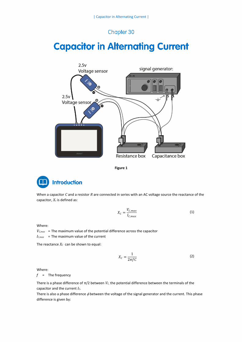
| Capacitor in Alternating Current |
Figure 1
When a capacitor C and a resistor R are connected in series with an AC voltage source the reactance of the
capacitor, Xc is defined as:
𝑋𝐶 =𝑉𝐶,𝑚𝑎𝑥
𝐼𝐶,𝑚𝑎𝑥
(1)
Where:
VC,max = The maximum value of the potential difference across the capacitor
IC,max = The maximum value of the current
The reactance XC can be shown to equal:
𝑋𝐶 =1
2𝜋𝑓𝐶 (2)
Where:
f = The frequency
There is a phase difference of π/2 between VC, the potential difference between the terminals of the
capacitor and the current IC.
There is also a phase difference between the voltage of the signal generator and the current. This phase
difference is given by:
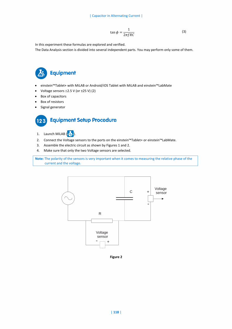
| Capacitor in Alternating Current |
| 118 |
tan 𝜙 =1
2𝜋𝑓𝑅𝐶 (3)
In this experiment these formulas are explored and verified.
The Data Analysis section is divided into several independent parts. You may perform only some of them.
einstein™Tablet+ with MiLAB or Android/iOS Tablet with MiLAB and einstein™LabMate
Voltage sensors 2.5 V (or ±25 V) (2)
Box of capacitors
Box of resistors
Signal generator
1. Launch MiLAB ( ).
2. Connect the Voltage sensors to the ports on the einstein™Tablet+ or einstein™LabMate.
3. Assemble the electric circuit as shown by Figures 1 and 2.
4. Make sure that only the two Voltage sensors are selected.
Note: The polarity of the sensors is very important when it comes to measuring the relative phase of the current and the voltage.
Figure 2
To input 1of MultiLog
+-
To input 2of MultiLog
Voltagesensor
Voltagesensor
R
C +
-
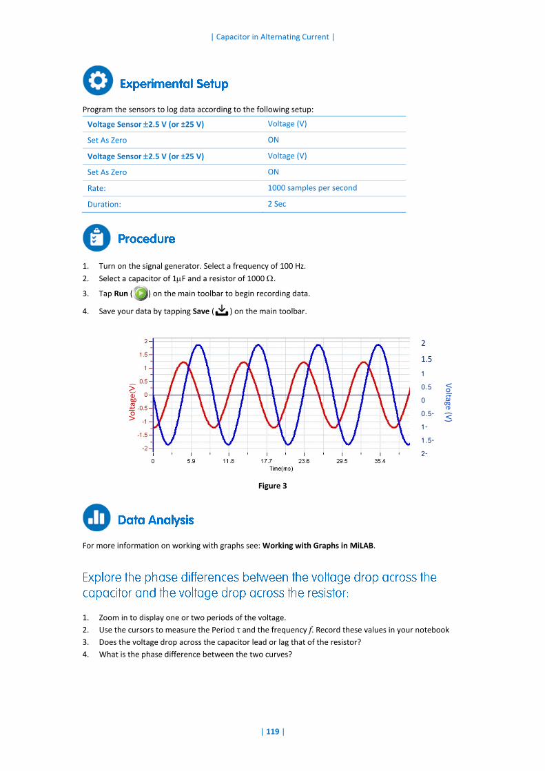
| Capacitor in Alternating Current |
| 119 |
Program the sensors to log data according to the following setup:
Voltage Sensor 2.5 V (or ±25 V) Voltage (V)
Set As Zero ON
Voltage Sensor 2.5 V (or ±25 V) Voltage (V)
Set As Zero ON
Rate: 1000 samples per second
Duration: 2 Sec
1. Turn on the signal generator. Select a frequency of 100 Hz.
2. Select a capacitor of 1F and a resistor of 1000 .
3. Tap Run ( ) on the main toolbar to begin recording data.
4. Save your data by tapping Save ( ) on the main toolbar.
Figure 3
For more information on working with graphs see: Working with Graphs in MiLAB.
1. Zoom in to display one or two periods of the voltage.
2. Use the cursors to measure the Period τ and the frequency f. Record these values in your notebook
3. Does the voltage drop across the capacitor lead or lag that of the resistor?
4. What is the phase difference between the two curves?
Vo
ltag
e (
V) Vo
ltage (V)
2
1.5
1
0.5
0
-0.5
-1
-1.5
-2
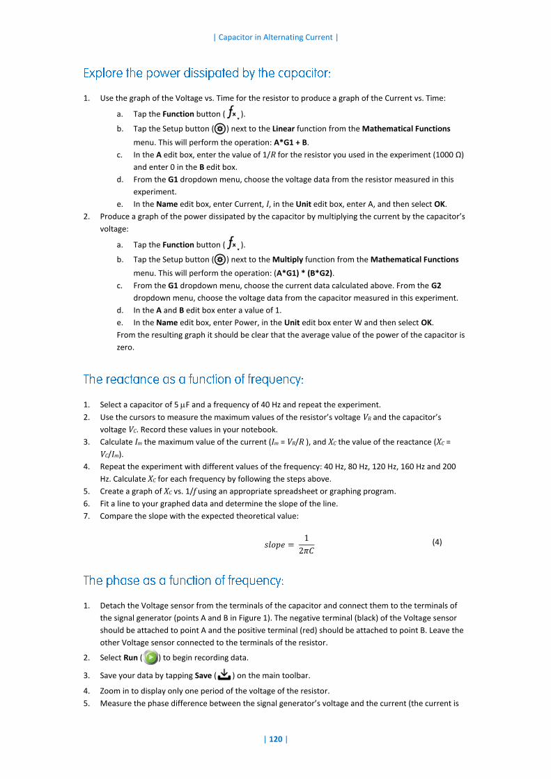
| Capacitor in Alternating Current |
| 120 |
1. Use the graph of the Voltage vs. Time for the resistor to produce a graph of the Current vs. Time:
a. Tap the Function button ( ).
b. Tap the Setup button ( ) next to the Linear function from the Mathematical Functions
menu. This will perform the operation: A*G1 + B.
c. In the A edit box, enter the value of 1/R for the resistor you used in the experiment (1000 Ω)
and enter 0 in the B edit box.
d. From the G1 dropdown menu, choose the voltage data from the resistor measured in this
experiment.
e. In the Name edit box, enter Current, I, in the Unit edit box, enter A, and then select OK.
2. Produce a graph of the power dissipated by the capacitor by multiplying the current by the capacitor’s
voltage:
a. Tap the Function button ( ).
b. Tap the Setup button ( ) next to the Multiply function from the Mathematical Functions
menu. This will perform the operation: (A*G1) * (B*G2).
c. From the G1 dropdown menu, choose the current data calculated above. From the G2
dropdown menu, choose the voltage data from the capacitor measured in this experiment.
d. In the A and B edit box enter a value of 1.
e. In the Name edit box, enter Power, in the Unit edit box enter W and then select OK.
From the resulting graph it should be clear that the average value of the power of the capacitor is
zero.
1. Select a capacitor of 5 F and a frequency of 40 Hz and repeat the experiment.
2. Use the cursors to measure the maximum values of the resistor’s voltage VR and the capacitor’s
voltage VC. Record these values in your notebook.
3. Calculate Im the maximum value of the current (Im = VR/R ), and XC the value of the reactance (XC =
VC/Im).
4. Repeat the experiment with different values of the frequency: 40 Hz, 80 Hz, 120 Hz, 160 Hz and 200
Hz. Calculate XC for each frequency by following the steps above.
5. Create a graph of XC vs. 1/f using an appropriate spreadsheet or graphing program.
6. Fit a line to your graphed data and determine the slope of the line.
7. Compare the slope with the expected theoretical value:
𝑠𝑙𝑜𝑝𝑒 = 1
2𝜋𝐶 (4)
1. Detach the Voltage sensor from the terminals of the capacitor and connect them to the terminals of
the signal generator (points A and B in Figure 1). The negative terminal (black) of the Voltage sensor
should be attached to point A and the positive terminal (red) should be attached to point B. Leave the
other Voltage sensor connected to the terminals of the resistor.
2. Select Run ( ) to begin recording data.
3. Save your data by tapping Save ( ) on the main toolbar.
4. Zoom in to display only one period of the voltage of the resistor.
5. Measure the phase difference between the signal generator’s voltage and the current (the current is
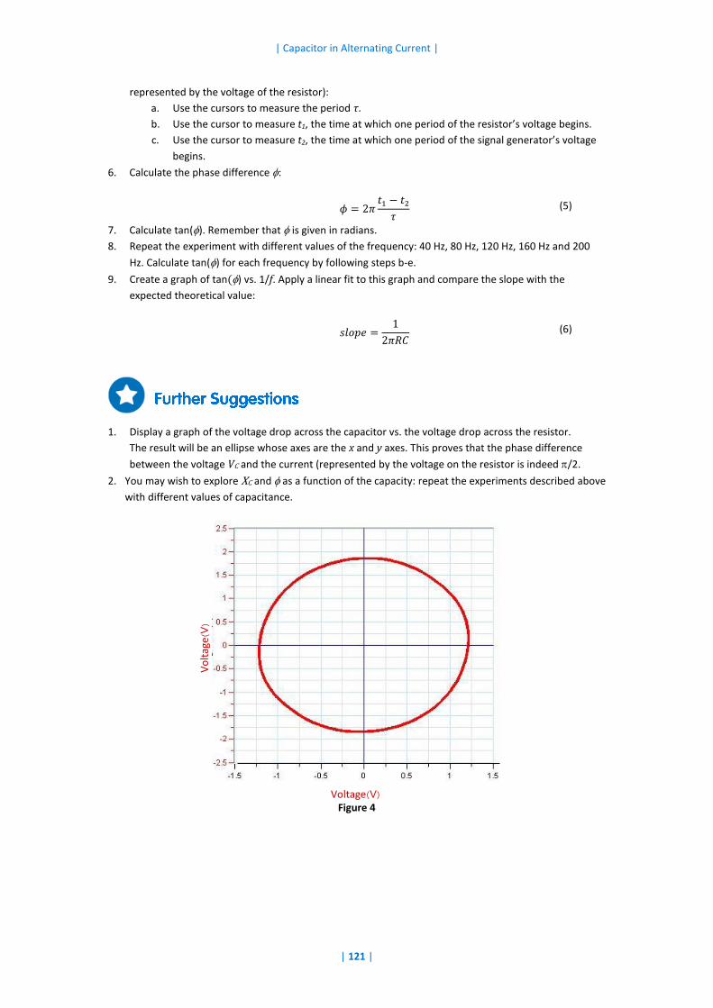
| Capacitor in Alternating Current |
| 121 |
represented by the voltage of the resistor):
a. Use the cursors to measure the period τ.
b. Use the cursor to measure t1, the time at which one period of the resistor’s voltage begins.
c. Use the cursor to measure t2, the time at which one period of the signal generator’s voltage
begins.
6. Calculate the phase difference :
𝜙 = 2𝜋𝑡1 − 𝑡2
𝜏 (5)
7. Calculate tan(). Remember that is given in radians.
8. Repeat the experiment with different values of the frequency: 40 Hz, 80 Hz, 120 Hz, 160 Hz and 200
Hz. Calculate tan() for each frequency by following steps b-e.
9. Create a graph of tan() vs. 1/f. Apply a linear fit to this graph and compare the slope with the
expected theoretical value:
𝑠𝑙𝑜𝑝𝑒 =1
2𝜋𝑅𝐶 (6)
1. Display a graph of the voltage drop across the capacitor vs. the voltage drop across the resistor.
The result will be an ellipse whose axes are the x and y axes. This proves that the phase difference
between the voltage VC and the current (represented by the voltage on the resistor is indeed /2.
2. You may wish to explore XC and as a function of the capacity: repeat the experiments described above
with different values of capacitance.
Figure 4
Vo
ltag
e (
V)
Voltage (V)
| Measuring the Speed of Sound |
Figure 1
In this experiment we measure the time it takes a sharp sound to travel the distance between two
microphones. The speed of sound is then calculated by dividing the distance between the
microphones by the time it took the sound to travel the distance between them.
In this manner the speed of sound in air, wood and metal can be measured.
einstein™Tablet+ with MiLAB or Android/iOS Tablet with MiLAB and einstein™LabMate
Microphone sensor (2)
Hammer
Optional:
o Long iron bar (2 m at least)
o Long aluminum bar (2 m at least)
o Long wooden surface (a 2 m long table will work well)
1. Launch MiLAB ( ).
2. Connect the Microphone sensors to two of the ports on the einstein™Tablet+ or einstein™LabMate.
3. Place the two microphones at least 2m apart, both facing the sound source (see Figure 1).
4. Make sure that only the Microphone sensors are selected.
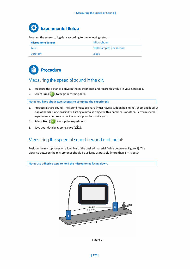
| Measuring the Speed of Sound |
| 123 |
Program the sensor to log data according to the following setup:
Microphone Sensor Microphone
Rate: 1000 samples per second
Duration: 2 Sec
1. Measure the distance between the microphones and record this value in your notebook.
2. Select Run ( ) to begin recording data.
Note: You have about two seconds to complete the experiment.
3. Produce a sharp sound. The sound must be sharp (must have a sudden beginning), short and loud. A
clap of hands is one possibility. Hitting a metallic object with a hammer is another. Perform several
experiments before you decide what option best suits you.
4. Select Stop ( ) to stop the experiment.
5. Save your data by tapping Save ( ).
Position the microphones on a long bar of the desired material facing down (see Figure 2). The
distance between the microphones should be as large as possible (more than 3 m is best).
Note: Use adhesive tape to hold the microphones facing down.
Figure 2
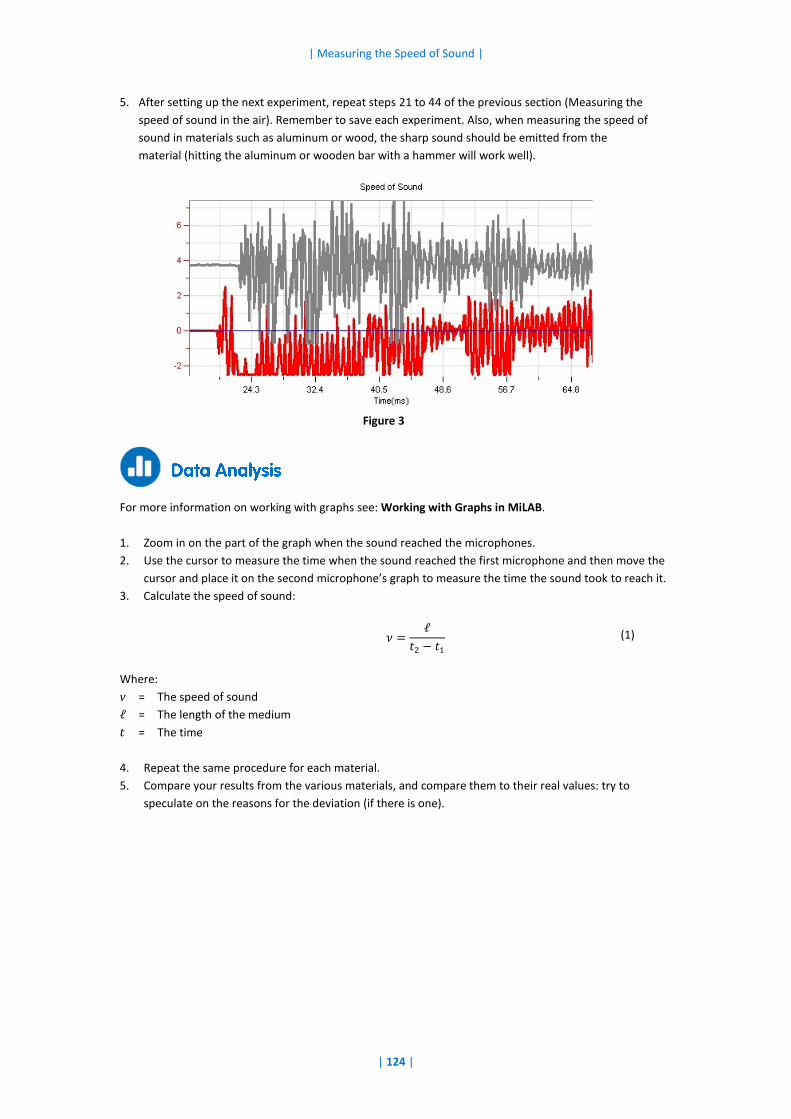
| Measuring the Speed of Sound |
| 124 |
5. After setting up the next experiment, repeat steps 21 to 44 of the previous section (Measuring the
speed of sound in the air). Remember to save each experiment. Also, when measuring the speed of
sound in materials such as aluminum or wood, the sharp sound should be emitted from the
material (hitting the aluminum or wooden bar with a hammer will work well).
Figure 3
For more information on working with graphs see: Working with Graphs in MiLAB.
1. Zoom in on the part of the graph when the sound reached the microphones.
2. Use the cursor to measure the time when the sound reached the first microphone and then move the
cursor and place it on the second microphone’s graph to measure the time the sound took to reach it.
3. Calculate the speed of sound:
𝜈 =ℓ
𝑡2 − 𝑡1
(1)
Where:
v = The speed of sound
ℓ = The length of the medium
t = The time
4. Repeat the same procedure for each material.
5. Compare your results from the various materials, and compare them to their real values: try to
speculate on the reasons for the deviation (if there is one).

Experiments in Physics for MiLAB™
imagine • explore • learnwww.einsteinworld.com
ALBERT EINSTEIN and EINSTEIN are either trademarks or registered trademarks of The Hebrew University of Jerusalem. Represented exclusively by GreenLight. Official licensed merchandise. Website: einstein.biz © 2014 Fourier Systems Ltd. All rights reserved. Fourier Systems Ltd. logos and all other Fourier product or service names are registered trademarks or trademarks of Fourier Systems. All other registered trademarks or trademarks belong to their respective companies. einstein™World LabMate, einstein™Activity Maker, MultiLab, MiLAB and Terra Nova, are registered trademarks or trademarks of Fourier Systems LTD. Second Edition, February 2015. Part Number: BK272
www.einsteinworld.com
USA8940 W. 192nd St.
Unit IMokenaIL 60448
Tel: (877) 266-4066
www.FourierEdu.com
Israel 16 Hamelacha St.POB 11681Rosh Ha’ayin 48091Tel: +972-3-901-4849 Fax: +972-3-901-4999
Experiments in Physics for M
iLAB