Experimental learning of quantum states

Andrea Rocchetto,1, 2, ∗ Scott Aaronson,3 Simone Severini,1, 4 Gonzalo Carvacho,5Davide Poderini,5 Iris Agresti,5 Marco Bentivegna,5 and Fabio Sciarrino5, †

1Department of Computer Science, University College London, London, UK2Department of Materials, University of Oxford, Oxford, UK

3Department of Computer Science, University of Texas at Austin, Austin, USA4Institute of Natural Sciences, Shanghai Jiao Tong University, Shanghai, China

5Dipartimento di Fisica - Sapienza Universita di Roma, Rome, Italy(Dated: December 4, 2017)

The number of parameters describing a quantum state is well known to grow exponentially withthe number of particles. This scaling clearly limits our ability to do tomography to systems withno more than a few qubits and has been used to argue against the universal validity of quantummechanics itself. However, from a computational learning theory perspective, it can be shown that,in a probabilistic setting, quantum states can be approximately learned using only a linear numberof measurements. Here we experimentally demonstrate this linear scaling in optical systems with upto 6 qubits. Our results highlight the power of computational learning theory to investigate quantuminformation, provide the first experimental demonstration that quantum states can be “probablyapproximately learned” with access to a number of copies of the state that scales linearly with thenumber of qubits, and pave the way to probing quantum states at new, larger scales.

The exponential scaling of the wavefunction, arisingfrom the tensor product description of multi-particlestates, is one of the remarkable properties of quantumsystems. If exploited correctly it can be used to achievethe computational advantages theorised in quantum in-formation processing, but it can also lead one to questionthe consistency of quantum mechanics itself: does it makesense at all to talk about objects with more parametersthan the number of atoms in the universe?

One of the problems arising from the exponential scal-ing of the wavefunction can be formalised in quantumtomography [1–8]. The central task of quantum tomogra-phy is to produce a description of an n-qubit state giventhe ability to prepare and measure k of its copies [6].Characterising an unknown quantum state is a fundamen-tal tool in quantum information processing. A survey ofthe major applications and present challenges in statetomography can be found in the review by Banaszek,Cramer, and Gross [1]. State estimation is, in general,an expensive procedure. For an n-qubit quantum stateit can be shown that estimating the ideal state up toan approximation parameter ε requires Ω(4n/ε2) opera-tions [2]. Although prior information, such as the statebeing low-rank, can be used to reduce the computationalcost of quantum tomography [3, 7, 8], there is no hope ofovercoming the exponential scaling for general unknownquantum states. Given this difficulty, it is valuable tointerpret quantum tomography as a learning problem,with the hope of using the well-developed machinery ofcomputational learning theory, for optimizing the numberof required measurements.

Computational learning theory [9, 10] is a research fielddevoted to studying the design and analysis of machine

∗ E-mail:andrea.rocchetto@spc.ox.ac.uk† E-mail:fabio.sciarrino@uniroma1.it

learning algorithms. Particularly relevant for our pur-poses is supervised machine learning. Here the learneris presented with a number of examples consisting ofinput-output pairs and is subsequently assigned the taskof predicting the output of a new input. This model oflearning has been formalised in computational learningtheory by Valiant in 1984 [11] with the introduction ofthe Probably Approximately Correct (PAC) model. Thisframework provides two indicators of the efficiency of alearner: the sample complexity and the time complexity.The first is the worst-case number of examples it uses toreach some target competency, while the second one is theworst-case running time of the learner. In this article weare concerned with the sample complexity of the problemof learning quantum states.

Quantum state tomography can be rephrased as a learn-ing problem in the following sense. A full tomographyrequires a complete set of measurements. Consider alearner that by looking at only a few measurements canpredict the outcome of any measurement made on thestate. It is easy to see that generating this hypothesisis equivalent to reconstructing the density matrix of thestate. Because quantum tomography requires an expo-nentially large number of measurements we might assumethat the same applies for the learning problem.

This apparent exponential scaling of the learning prob-lem for quantum states can be interpreted as formalisingthe objections of quantum mechanics sceptics (for a criti-cal discussion see [12]). Indeed, one of the fundamentaltasks of science is to come up with hypotheses that, byexplaining past observations, let us predict future obser-vations. A theory that requires an exponentially growingnumber of observations to produce its hypothesis maysignal a problem with the theory itself.

Computational learning theory, and in particular thePAC model, can help to address these conundrums. Byanalysing quantum tomography from a computational

arX

iv:1

712.

0012

7v1

[qu

ant-

ph]

30

Nov

201

7

2

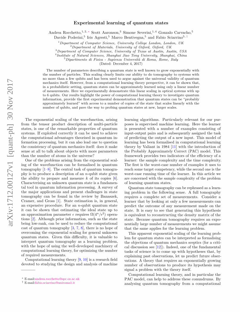
FIG. 1. Schematic of the learning procedure. In thelearning phase (top panel) measurements drawn randomlyfrom D are performed on the physical state ρ. Based on themeasurement outcomes the learning algorithm outputs anhypothesis σ. In the prediction phase (bottom panel) the goalis to predict the experimental outcome of a measurement E′drawn from D using σ as hypothesis.

learning perspective, Aaronson [13] proved that quantumstates can be PAC-learned with a linearly scaling trainingset. Here we present the first experimental demonstrationof such linear scaling. Our contributions also includedeveloping a testable model for the main theorem provedin [13] and estimating an important scaling constant. Werun the experiments on a photonic platform including upto 6 qubits. Our results demonstrate experimentally animportant property of quantum states and highlight thepower of computational learning theory in the quantuminformation framework.

QUANTUM LEARNABILITY THEORY

Let us recall some standard definitions in quantumtheory. A generic n-qubit state ρ is a trace-one, pos-itive semidefinite matrix acting on a Hilbert space ofdimension 2n. Every observation of a state is mathemati-cally described by a positive operator valued measurement(POVM), E = E(j), where each E(j) is a Hermitianpositive semidefinite operator such that

∑j E

(j) = I. Theprobability of measurement outcome j is p(j) =Tr(E(j)ρ).For our purposes, we refer to a measurement of ρ asa two-outcome POVM E(1) = E,E(2) = 1 − E witheigenvalues in [0, 1]. We denote by S the set of all mea-

surements on n qubits.Following Ref. [13] we define the learning of ρ as the

task of processing a training set composed of m tuples(Ei,Tr(Eiρ)), drawn from a probability distribution D,in order to predict the “behaviour” of ρ on most measure-ments drawn from D. This concept of learning is definedin the context of Valiant’s PAC model [11]. In this frame-work, originally developed for Boolean functions but thenextended to real-valued ones by Barlett and Long [14], alearning algorithm (the learner) tries to approximate withhigh probability an unknown function f : X → Y from atraining set of random labelled examples. Each labelledexample is of the form (x, f(x)), where x is distributedaccording to some unknown distribution D. In order tomake learning possible we restrict the hypothesis that thelearner can use to approximate f to a set of functionsH = h : X → Y. We refer to H as the hypothesis class.The learning algorithm takes as input the training set andgenerates a hypothesis h ∈ H that approximates f . ThePAC model makes use of two approximation parameters,ε and δ. The accuracy parameter ε determines how far thehypothesis h can be from f . The confidence parametergives the probability of sampling a training set that isnot representative of the underlying distribution D. Ahypothesis class H is said to be PAC-learnable if thereexists an algorithm that, for every probability distributionD and function f and for every ε,δ ∈ (0, 1), when runningthe learning algorithm on m ≥ mH examples drawn fromD, we have that, with probability at least 1− δ,

Prx∼D

[σ(x) 6= f(x)] ≤ ε.

Here by ∼ we indicate that x is drawn from D. Thevalue mH determines the minimum number of examplesrequired to PAC-learn the class H. We refer to mH asthe sample complexity of the hypothesis class H. Wenote that the learner must test the predictions under thesame distribution D that determines the elements in thetraining set.

The PAC-model has been adapted to quantum statesin [13]. Here the learner tries to approximate a func-tion Fρ : S → [0, 1] where Fρ is defined as Fρ(E(1)

i ) =Tr(E(1)

i ρ). The training set corresponds to a set of mtuples (E(1)

i , Fρ(E(1)i )). Notice that we always take the

first element E(1)i of each POVM Ei. For this reason,

in the following, we take E(1)i = Ei. The POVM mea-

surements Ei are drawn from an unknown distributionD and the Fρ(Ei) values are determined experimentally.After processing the training set the learner outputs ahypothesis state σ. A quantum state is considered to belearned if, with probability 1− δ, a training set generatedaccording to the distribution D can be used to predictwith probability ε and accuracy γ any other measurementdrawn from D:

PrE∈D

[|Tr (Eσ)− Tr (Eρ)| > γ] ≤ ε. (1)

A pictorial description of this learning procedure is shown

3

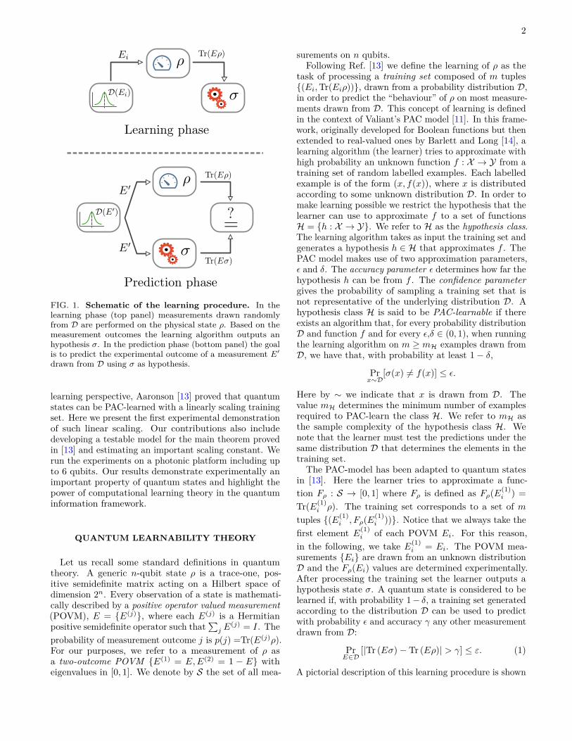
FIG. 2. Experimental setups for generating the 3, 4, 5 and 6-qubit GHZ states. Pictorial representation of the twodifferent experimental setups used to generated the quantum states learned with Theorem 1. In setup (I) we makes use oftwo photons and encode up to 4 qubits. In setup (II) we makes use of four photons and encode up to 6 qubits. (I) In thegeneration stage, the state of each of the two entangled photons (1 and 2) is locally manipulated via QWPs, HWPs and q-plates,set to generate a specific GHZ state. The analysis is performed using QWPs, HWPs and PBSs. The OAM analysis requires aq-plate to transfer the information encoded in the OAM space to the polarisation degree of freedom which can be then analysedwith standard techniques. After the analysis, both photons are sent to single mode fibres connected to single photon detectors.(II) Two polarization-entangled photon pairs are generated via SPDC in two separated non-linear crystals. Photon A and Dof the first and second pair respectively are sent directly to a HWP and a PBS for polarisation analysis. Photons B and Cinstead are sent to a 50/50 in-fiber PBS followed by another PBS which realizes the polarisation-path entanglement. The twopaths go through two HWP and are rejoined in the same PBS forming a Sagnac-like configuration which allow us to performpolarisation and path analysis without worrying about phase instabilities. A motorized delay line is adopted to change thephotons wave-packet temporal overlap in the PBS. The path analysis section is composed by HWP and PBS after which thephotons are coupled into SM fibres connected to single photon detectors. Generation and analysis sections are represented bycyan and grey zones, respectively.

in Fig. 1. Because σ is a 2n × 2n-dimensional matrix wewould expect that the number of examples in the trainingset required to learn ρ also scales exponentially. However,it has been proved [13] that the number of examplesrequired to learn Fρ scales linearly with n and inversepolynomially with the relevant error parameters (a fullstatement of the theorem is given in Methods. In thefollowing we shall refer to theorem as Theorem 1). Morespecifically, fixed the error parameters ε, γ and δ, we canPAC-learn a quantum state provided:

m ≥ K

γ4ε2

(n

γ4ε2 log2 1γε

+ log 1δ

), (2)

where K is a constant. This result provides an upperbound on the number of measurements required to learn

a quantum state with respect to any probability measureover two-outcome POVM measurements. The value ofK is left unbounded but it is critical for applying thetheorem in an experimental setting.

The learning procedure prescribed by Theorem 1 issimple and it involves finding a hypothesis state σ suchthat Tr(Eiσ) ≈ Tr(Eiρ) for all i. Then, with high prob-ability, that hypothesis will generalise in the sense thatTr(Eσ) ≈ Tr(Eρ) for most E’s drawn from D. It isthen possible to interpret the problem of finding a mixedn-qubit state which approximately agrees with the mea-surements as an optimisation problem.

The optimisation problem takes as input mPOVM measurements described by Hermitian matricesE1, . . . , Em and their corresponding measurement out-

4

N of qubits Experimental Setup PhotonA B C D

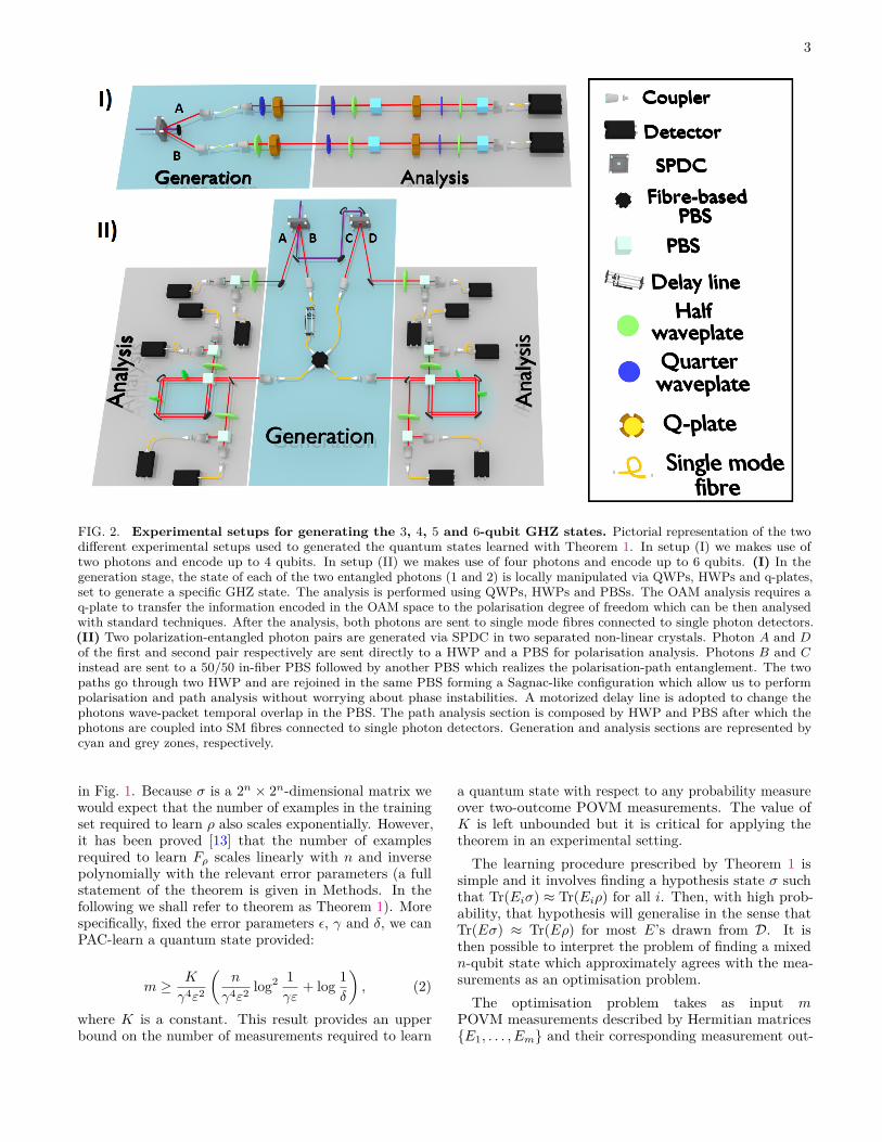
|0〉1 = |H〉 |0〉2 = |H〉2 I |1〉1 = |V 〉 |1〉2 = |V 〉|0〉1 = |R〉 |0〉2 = |+1〉 |0〉3 = |R〉3 I |1〉1 = |L〉 |1〉2 = |−1〉 |1〉3 = |L〉|0〉1 = |R〉 |0〉2 = |+1〉 |0〉3 = |R〉 |0〉4 = |+1〉4 I |1〉1 = |L〉 |1〉2 = |−1〉 |1〉3 = |L〉 |1〉4 = |−1〉|0〉1 = |H〉 |0〉2 = |H〉 |0〉3 = |H〉3 II |1〉1 = |V 〉 |1〉2 = |V 〉 |1〉3 = |V 〉|0〉1 = |H〉 |0〉2 = |H〉 |0〉3 = |H〉 |0〉4 = |H〉4 II |1〉1 = |V 〉 |1〉2 = |V 〉 |1〉3 = |V 〉 |1〉4 = |V 〉|0〉1 = |H〉 |0〉2 = |a〉 |0〉3 = |H〉 |0〉4 = |H〉 |0〉5 = |H〉5 II |1〉1 = |V 〉 |1〉2 = |b〉 |1〉3 = |V 〉 |1〉4 = |V 〉 |1〉5 = |V 〉|0〉1 = |H〉 |0〉2 = |a〉 |0〉3 = |H〉 |0〉4 = |a〉 |0〉5 = |H〉 |0〉6 = |H〉6 II |1〉1 = |V 〉 |1〉2 = |b〉 |1〉3 = |V 〉 |1〉4 = |b〉 |1〉5 = |V 〉 |1〉6 = |V 〉

TABLE I. Qubit encoding. The table shows the encoding map between logical states and photons. Photons are labeled withcapital letters A, B, C and D. Two photons (A and B in the table) are used in setup (I) to encode states up to 4 qubits in thepolarisation and OAM basis. For setup (II) states up to 6-qubits are generated adding two extra photons (C and D) and usingan encoding in path and polarisation. The states |H〉 , |V 〉 , |R〉 , |L〉 denote the polarisation degree of freedom while |+1〉 and|−1〉 represent the eigenstates of the OAM with l = +1 and l = −1, respectively. To identify the two possible paths of thephotons in setup (II) we use the labels |a〉 and |b〉.

comes Tr(E1ρ), . . . ,Tr(Emρ). The goal is to find anHermitian positive semidefinite matrix σ that minimises

f(σ) =m∑i=1

(Tr(Eiσ)− Tr(Eiρ))2 (3)

σ 0, Tr(σ) = 1,

where by σ 0 we denote the positive semidefinitenessof σ.

The above formulation is a convex program whose solu-tion is known to be computable in polynomial time in thedimension of σ using interior point methods [15, 16] or theellipsoid method [17]. However, because the dimension ofσ scales exponentially with n, the problem of finding theminimum of f(σ) is in practice not efficiently computable.This is still compatible with the linear scaling of Theo-rem 1 (see Methods) because the results proved in [13]are purely information-theoretic and are concerned onlywith the sample size m. For any given class of quantumstates, the question is still open of whether hypothesisstates can be produced efficiently. In this context, Roc-chetto recently proved that stabiliser states are efficientlyPAC-learnable [18].

Finally, we note that learning a quantum state is nota complete replacement for standard quantum state to-mography. The PAC-learning framework of Theorem 1tests the predictions over the same distribution of thetraining set; a good hypothesis state could be arbitrarilyfar from the true state in the usual trace distance metric,but hard to distinguish from the true state with respectto the given distribution over measurements.

EXPERIMENTAL SETUP

We test the learning Theorem 1 over differentGreenberger-Horne-Zeilinger (GHZ) states [19] (seeMethods for a definition). There are several methodsto produce GHZ states [20–28] in photonic systems.In order to scale up to 6 qubits we use two differentapproaches: the first one aims to increase the numberof degrees of freedom per photon while the second oneexploits an increasing number of photons (see Fig. 2).In setup (I) we generate 2-photon states, encoding upto 4 qubits, and perform a full set of measurementsin the computational basis. In setup (II) we generatefour-photon states, able to encode up to 6 qubits. Bothsetups exploit spontaneous parametric down conversion(SPDC) in order to generate polarisation-entangledphotons pairs (see Methods).

In setup (I), depicted in Fig. 2, we use the q-plate [29],a birefringent patterned slab, to entangle polarisation andorbital angular momentum (OAM) of single photons [30–33]. This makes possible to encode 2 qubits per photon,exploiting their polarisation and OAM degrees of freedom.In order to obtain a 4-qubit GHZ state, the q-plate actson the Bell state |ψ−〉 = 1√

2 (|RL〉 − |LR〉), where Rand L denote, respectively, the right and left circularpolarisation of the two photons, allowing a polarisation–controlled variation of the OAM. More specifically, stateswith right or left polarisation become OAM eigenstateswith ` = −1 or ` = +1 respectively. Conditioned on themeasurements of a subset of qubits, we can also generate3- and 2-qubit states, as summarized in table I. In orderto perform a complete quantum state tomography in bothHilbert spaces, the analysis is carried out using two series

5

FIG. 3. Learning of a 4-qubit GHZ state. Numerical simulations (blue curves) and experimental data (red curves) ofthe learning of the state (|0000〉+ |1111〉) /

√2. (left) The probability ε of predicting a measurements with less than γ = 0.1

accuracy. The black line represents the predictions made using the completely mixed state as hypothesis. Clearly, the informedpredictions are always better than a random guess. (right) The distance, in terms of the fidelity F =

√σ1/2ρσ1/2, between the

hypothesis state σ and ρ and between σ and the completely mixed state I/2n, starting guess of the optimisation algorithm. Adiscussion on the high variance of the datapoints with m = 4 is provided in the Methods section. The learning distribution D(I)is uniform over the set of stabiliser measurements of the state minus the identity matrix (see Methods). Every datapoint is anaverage of 20 different, randomly generated, sets of measurement configurations.

of quarter-wave plates (QWP), half-wave plates (HWP)and polarising beam splitters (PBS), separated by anotherq-plate, to transfer the information from the OAM to thepolarisation subspace [33]. The photons are then sent tosingle mode fibres (SMF), which can be coupled only withstates carrying null OAM.

In setup (II), depicted in Fig. 2, we encode the qubitsin the polarisation and path degrees of freedom. Throughthis encoding we can generate 4-photon states and up to6-qubit. This setup involves two separate SPDC sources,which generate two pairs of polarisation-entangled pho-tons, (A,B) and (C,D), with the same pulse of the laser.We can then obtain a 4-qubit GHZ state encoded in po-larisation, by simultaneously injecting one photon fromeach source (B and C) over the two inputs of a fibre-basedPBS. In this configuration, each photon carries one qubit.The dimension of the system can be increased to 5 qubitsby sending one of the two output modes of the fibre-basedPBS in a Sagnac interferometer (shown in Fig. 2). Thisallows us to entangle and measure the polarisation andpath degrees of freedom of a single photon while retainingphase stability. This scheme can be easily extended to 6qubits by sending the other output mode of fibre-basedPBS in another Sagnac interferometer. In this case, twoout of the four photons carry 2 qubits, which are encodedin the polarisation and path degree of freedom, as shownin Table I. Through the above procedures we can generatethe state

|GHZn〉 = 1√2

(|0〉⊗n + |1〉⊗n

)(4)

for n = 3, 4, 5, 6 qubits. The polarisation analysis is

performed with a HWP and a PBS for each path.

EXPERIMENTAL DEMONSTRATION

We demonstrate numerically and experimentally,through two photonic systems able to encode from 2 to 6qubits, that quantum states can be PAC-learned with alinearly scaling training set: that is, we demonstrate thatthe number of elements m in the training set required tolearn an n-qubit quantum state ρ scales linearly with n.

Although Theorem 1 can be applied under any distri-bution D, it is interesting to test its prediction underdistributions that include measurements that are difficultto predict. If, for example, one were to take the uniformdistribution over all possible measurement bases, withhigh probability no measurement drawn from this distri-bution would be able to distinguish the state from thecompletely mixed one. We define the completely mixedstate as the state described by the density matrix I/2n,where by I we denote the identity matrix.

All of our experiments are performed on GHZ states, atype of stabiliser state (see Methods for further details).We remark that the validity of Theorem 1 extends to allquantum states. The advantage of using GHZ states isthe possibility of clearly identifying a set of measurementsand a probability distribution that make the predictionsof theorem “interesting” in the sense that they cannot bereproduced using the completely mixed state as hypoth-esis. Depending on the experimental setup we use two

6

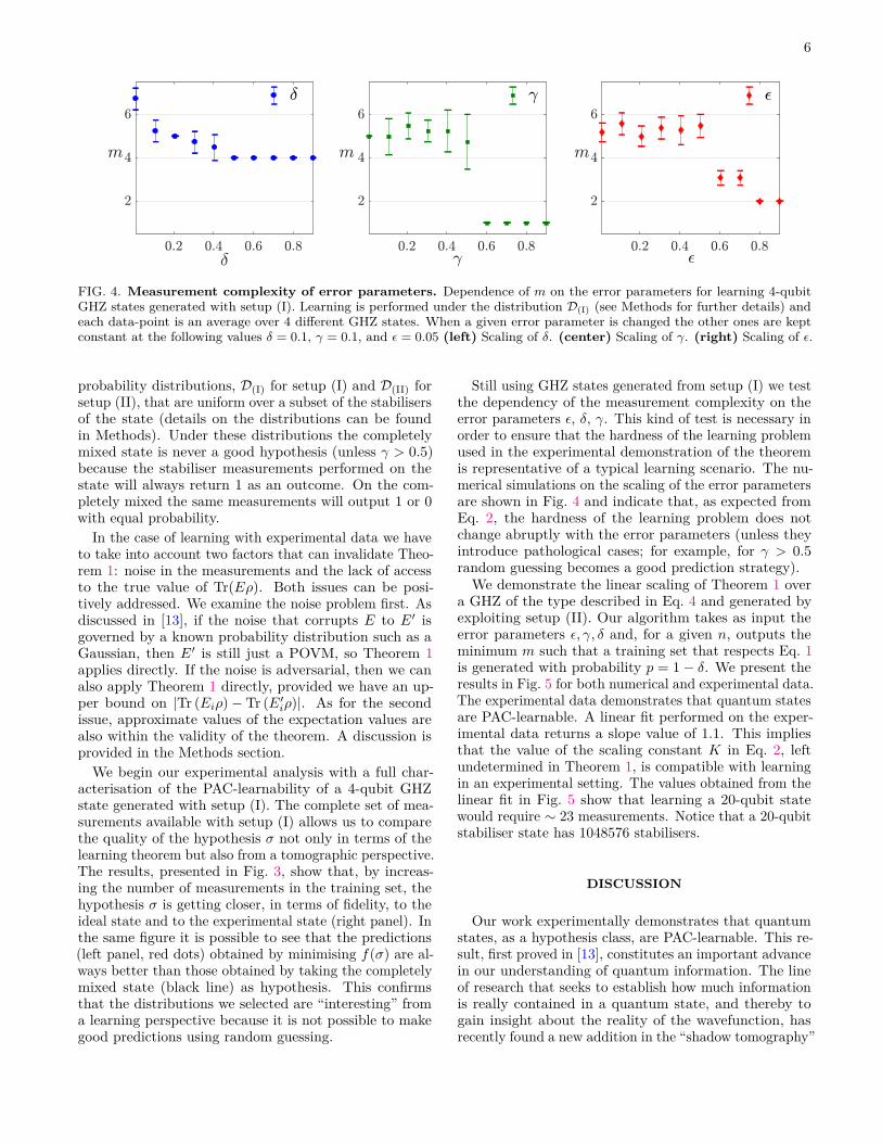
FIG. 4. Measurement complexity of error parameters. Dependence of m on the error parameters for learning 4-qubitGHZ states generated with setup (I). Learning is performed under the distribution D(I) (see Methods for further details) andeach data-point is an average over 4 different GHZ states. When a given error parameter is changed the other ones are keptconstant at the following values δ = 0.1, γ = 0.1, and ε = 0.05 (left) Scaling of δ. (center) Scaling of γ. (right) Scaling of ε.

probability distributions, D(I) for setup (I) and D(II) forsetup (II), that are uniform over a subset of the stabilisersof the state (details on the distributions can be foundin Methods). Under these distributions the completelymixed state is never a good hypothesis (unless γ > 0.5)because the stabiliser measurements performed on thestate will always return 1 as an outcome. On the com-pletely mixed the same measurements will output 1 or 0with equal probability.

In the case of learning with experimental data we haveto take into account two factors that can invalidate Theo-rem 1: noise in the measurements and the lack of accessto the true value of Tr(Eρ). Both issues can be posi-tively addressed. We examine the noise problem first. Asdiscussed in [13], if the noise that corrupts E to E′ isgoverned by a known probability distribution such as aGaussian, then E′ is still just a POVM, so Theorem 1applies directly. If the noise is adversarial, then we canalso apply Theorem 1 directly, provided we have an up-per bound on |Tr (Eiρ)− Tr (E′iρ)|. As for the secondissue, approximate values of the expectation values arealso within the validity of the theorem. A discussion isprovided in the Methods section.

We begin our experimental analysis with a full char-acterisation of the PAC-learnability of a 4-qubit GHZstate generated with setup (I). The complete set of mea-surements available with setup (I) allows us to comparethe quality of the hypothesis σ not only in terms of thelearning theorem but also from a tomographic perspective.The results, presented in Fig. 3, show that, by increas-ing the number of measurements in the training set, thehypothesis σ is getting closer, in terms of fidelity, to theideal state and to the experimental state (right panel). Inthe same figure it is possible to see that the predictions(left panel, red dots) obtained by minimising f(σ) are al-ways better than those obtained by taking the completelymixed state (black line) as hypothesis. This confirmsthat the distributions we selected are “interesting” froma learning perspective because it is not possible to makegood predictions using random guessing.

Still using GHZ states generated from setup (I) we testthe dependency of the measurement complexity on theerror parameters ε, δ, γ. This kind of test is necessary inorder to ensure that the hardness of the learning problemused in the experimental demonstration of the theoremis representative of a typical learning scenario. The nu-merical simulations on the scaling of the error parametersare shown in Fig. 4 and indicate that, as expected fromEq. 2, the hardness of the learning problem does notchange abruptly with the error parameters (unless theyintroduce pathological cases; for example, for γ > 0.5random guessing becomes a good prediction strategy).

We demonstrate the linear scaling of Theorem 1 overa GHZ of the type described in Eq. 4 and generated byexploiting setup (II). Our algorithm takes as input theerror parameters ε, γ, δ and, for a given n, outputs theminimum m such that a training set that respects Eq. 1is generated with probability p = 1− δ. We present theresults in Fig. 5 for both numerical and experimental data.The experimental data demonstrates that quantum statesare PAC-learnable. A linear fit performed on the exper-imental data returns a slope value of 1.1. This impliesthat the value of the scaling constant K in Eq. 2, leftundetermined in Theorem 1, is compatible with learningin an experimental setting. The values obtained from thelinear fit in Fig. 5 show that learning a 20-qubit statewould require ∼ 23 measurements. Notice that a 20-qubitstabiliser state has 1048576 stabilisers.

DISCUSSION

Our work experimentally demonstrates that quantumstates, as a hypothesis class, are PAC-learnable. This re-sult, first proved in [13], constitutes an important advancein our understanding of quantum information. The lineof research that seeks to establish how much informationis really contained in a quantum state, and thereby togain insight about the reality of the wavefunction, hasrecently found a new addition in the “shadow tomography”

7

FIG. 5. Experimental demonstration of Theorem 1.Scaling of size of the training set m required to learn a GHZstate as a function of the number of qubits n. Experimentaldata-points (red crosses) are obtained using the experimentalsetup (II). Each data-point is obtained using 50 different,randomly generated sets of measurement configurations drawnfrom D(II) (see Methods for further details). Error bars showthe standard deviation for an average of 10 different runs ofthe algorithm to estimate m. The red line is a linear fit onthe experimental data-points with equation m = 1.19n− 0.34.The learning parameters are ε = 0.15, γ = 0.2 and δ = 0.2.

protocol proposed by Aaronson [34]. This protocol canpredict the outcomes of M different two-outcome mea-surements on a D-dimensional state, to high accuracy, bymeasuring only poly(log(D), log(M)) copies of the state.An experimental demonstration of this protocol is a natu-ral future direction, and would be a valuable addition toour physical comprehension of these theoretical results.

From a broader perspective, our work constitutes an

example of how the techniques developed in the frame-work of computational learning theory can be used withinquantum information. The interplay of these two fields,recently surveyed by Arunachalam and de Wolf [35], canoffer new tools to investigate properties of quantum statesand circuits and can help to identify cases in machinelearning where classical and quantum computation be-have differently. This is particularly important in light ofthe recent advances in quantum algorithms for machinelearning (recently reviewed by Biamonte et al. [36] and byCiliberto et al. [37]) where, despite the growing interest forthe topic, it is still unclear whether caveat-free speedupscan be attained (for a critical discussion see [37, 38]).

Acknowledgments

This work was initiated at the Aspen Center for Physics,which is supported by National Science Foundation grantPHY-1066293. The authors would like to thank SimonBenjamin and Ying Li for useful discussions and com-ments on the manuscript. This work was supported bythe ERC-Starting Grant 3D-QUEST (3D-Quantum Inte-grated Optical Simulation; grant agreement no. 307783):http://www.3dquest.eu. AR is supported by an EPSRCDTP Scholarship and by QinetiQ Ltd. SA is supportedby a Vannevar Bush Faculty Fellowship from the USDepartment of Defense. SS is supported by The Royal So-ciety, EPSRC, the National Natural Science Foundationof China, and the grant ARO-MURI W911NF-17-1-0304(US DOD, UK MOD and UK EPSRC under the Multidis-ciplinary University Research Initiative). GC is supportedby Becas Chile and Conicyt. The authors would like toacknowledge the use of the University of Oxford AdvancedResearch Computing (ARC) facility in carrying out thiswork http://dx.doi.org/10.5281/zenodo.22558.

[1] Banaszek, K., Cramer, M., & Gross, D. Focus on quantumtomography. New Journal of Physics 15, 125020 (2013).

[2] Haah, J., Harrow, A. W., Ji, Z., Wu, X. & Yu, N. Sample-optimal tomography of quantum states, IEEE Transac-tions on Information Theory 63, 5628–5641 (2017).

[3] Gross, D., Liu, Y. K., Flammia, S. T., Becker, S., & Eisert,J. Quantum state tomography via compressed sensing.Physical review letters 105, 150401 (2010).

[4] D’Ariano, G. M., Paris, M. G. A., Sacchi, M. F. QuantumTomography. Advances in Imaging and Electron Physics128, (2003).

[5] Agnew, M., Leach, J., McLaren, M., Roux, F. S., & Boyd,R. W. Tomography of the quantum state of photonsentangled in high dimensions. Phys. Rev. A 84, (2011).

[6] Lvovsky, A.I. and Raymer, M.G. Continuous-variableoptical quantum-state tomography, Reviews of ModernPhysics 81.1, 299 (2009).

[7] Cramer, M., et al. Efficient quantum state tomography.Nature communications 1, 149 (2010).

[8] O’Donnell, R. & Wright, J. Efficient quantum tomography.Proceedings of the 48th Annual ACM SIGACT Symposiumon Theory of Computing, 899-912, (2016).

[9] Kearns, M. J., & Vazirani, U. V. An introduction tocomputational learning theory (MIT press, Chicago, 1994).

[10] Shalev-Shwartz, S., & Ben-David, S. Understanding ma-chine learning: From theory to algorithms (CambridgeUniversity Press, Cambridge, 2014).

[11] Valiant, L. G. A theory of the learnable. Communicationsof the ACM 27.11, 1134-1142, (1984).

[12] Aaronson, S. Quantum computing since Democritus (Cam-bridge University Press, Chicago 2013).

[13] Aaronson, S. The learnability of quantum states. Pro-ceedings of the Royal Society of London A: Mathemati-cal, Physical and Engineering Sciences 2088, 3089-3114,(2007).

[14] Bartlett, P. L., Long, P. M., & Williamson, R. C. Fat-shattering and the learnability of real-valued functions.Proceedings of the seventh annual conference on Compu-

8

tational learning theory, 299-310, (1994).[15] Nesterov, Y., & Nemirovskii, A. Interior-point polyno-

mial algorithms in convex programming (Vol. 13) (SIAM,Philadelphia, 1994).

[16] Alizadeh, F. Interior point methods in semidefinite pro-gramming with applications to combinatorial optimiza-tion. SIAM Journal on Optimization 5, 13-51 (1995).

[17] Grotschel, M., Lovasz, L., & Schrijver, A. Geometric algo-rithms and combinatorial optimization (Vol. 2) (SpringerScience & Business Media, Heidelberg, 2012).

[18] Rocchetto, A. Stabiliser states are efficiently PAC-learnable. Preprint at https://arxiv.org/abs/1705.00345(2017).

[19] Greenberger, D. M., Horne, M. A., & Zeilinger, A. Goingbeyond Bell’s theorem. Bell’s theorem, quantum theoryand conceptions of the universe 69-72. (Springer Nether-lands, 1989).

[20] Walther, P., Resch, K. J., Brukner, C. & Zeilinger, A.Experimental entangled entanglement. Physical reviewletters 97, 020501 (2006).

[21] Huang, Y.-F., et al. Experimental generation of an eight-photon Greenberger-Horne-Zeilinger state. Nature com-munications 2, 546 (2011).

[22] Leibfried, D., et al., Toward heisenberg-limited spec-troscopy with multiparticle entangled states. Science 304,1476-1478 (2004).

[23] Brattke, S., Varcoe, B. T. H. & Walther, H. Generationof photon number states on demand via cavity quantumelectrodynamics. Physical review letters 86, 3534-3537(2001).

[24] Carvacho, G., Graffitti, F., D’Ambrosio, V., Hiesmayr,Beatrix C. & Sciarrino, F. Experimental investigation onthe geometry of GHZ states. Scientific Reports 7, 13265(2017).

[25] Gao, W.B., et al. Experimental demonstration of a hyper-entangled ten-qubit Schrodinger cat state. Nature Physics6, 331-335 (2010).

[26] Ciampini, M.A., et al. Path-polarization hyperentangledand cluster states of photons on a chip. Light: Scienceand Applications 5, (2016).

[27] Barreiro, J.T., Langford, N.K., Peters, N.A.& Kwiat, P.G.Generation of hyperentangled photon pairs. Phys. Rev.Lett. 95, (2005).

[28] Barbieri, M., Cinelli, C., Mataloni, P. & De Martini,F. Polarization-momentum hyperentangled states: Real-ization and characterization. Phys. Rev. A 72, 052110(2005).

[29] Piccirillo, B., D’Ambrosio, V., Slussarenko, S., Marrucci,L. & Santamato, E. Photon spin-to-orbital angular mo-mentum conversion via an electrically tunable q-plate.Applied Physics Letters 97, (2010).

[30] D’Ambrosio, V., et al. Entangled vector vortex beams.Phys. Rev. A 94, (2016).

[31] Marrucci, L., Manzo, C. & Paparo, D. Optical spin-to-orbital angular momentum conversion in inhomogeneousanisotropic media. Physical review letters 96, 163905(2006).

[32] Marrucci, L., et al. Spin-to-orbital conversion of the an-gular momentum of light and its classical and quantumapplications. Journal of Optics 13, (2011).

[33] Nagali, E., et al. Quantum information transfer from spinto orbital angular momentum of photons. Physical reviewletters 103, 013601 (2009).

[34] Aaronson, S. Shadow Tomography of Quantum States.Preprint at https://arxiv.org/abs/1711.01053 (2017).

[35] Arunachalam, S., & de Wolf, R. Guest Column: A Surveyof Quantum Learning Theory. SIGACT News 48.2, 41-67(2017).

[36] Biamonte, J., et al. Quantum machine learning. Nature549, 195-202 (2017).

[37] Ciliberto, C., et al. Quantum machine learning: a classicalperspective. Preprint at https://arxiv.org/abs/1707.08561(2017).

[38] Aaronson, S. Read the fine print. Nature Physics 11,291-293 (2015).

[39] Gottesman, D. Class of quantum error-correcting codessaturating the quantum Hamming bound. Physical ReviewA 54, 1862 (1996).

[40] Frank, M., & Wolfe, P. An algorithm for quadratic pro-gramming. Naval research logistics quarterly 3, 95-110,(1956).

[41] Hazan, E. Sparse approximate solutions to semidefiniteprograms. Latin American Symposium on Theoretical In-formatics, 306-316. (Springer, Heidelberg).

9

METHODS

The learning theorem

The theorem proved in Ref. [13] states:

Theorem 1. Let ρ be an n-qubit state, let D be adistribution over two-outcome measurements, and letE = (E1, . . . , Em) consist of m measurements drawn in-dependently from D. Suppose we are given bits B =(b1, . . . , bm), where each bi is 1 with independent probabil-ity Tr (Eiρ) and 0 with probability 1−Tr (Eiρ). Supposealso that we choose a hypothesis state σ to minimize thequadratic functional f(σ) =

∑mi=1 (Tr (Eiσ)− bi)2. Then

there exists a positive constant K such that

PrE∈D

[|Tr (Eσ)− Tr (Eρ)| > γ] ≤ ε

with probability at least 1− δ over E and B, provided that

m ≥ K

γ4ε2

(n

γ4ε2 log2 1γε

+ log 1δ

).

In this article, rather than working with single mea-surement outcomes bi, we are concerned with estimatedexpected values

Tr (Eiρ) ≈S∑j=1

b(j)i /S

where each b(j)i is the j-th measurement outcome corre-

sponding to Ei. In order to show that the hypothesis σgenerated by considering the expected values is equivalentto that obtained by taking the measurements outcome bi,we define

f ′ =m′∑i=1

(Tr (Eiσ)− Tr (Eiρ))2.

If we take m = m′S and solve for σ the equations df/dσ =0 and df ′/dσ = 0 it is possible to verify that the hypothesisthat minimises the function f ′ is also satisfying f .

The learning distributions

We use different learning distributions for the two ex-perimental setups, D(I) and D(II). The distribution D(I) isuniform over the set of stabiliser measurements [39] of theGHZ state minus the identity matrix. The distributionD(II) is uniform over the set of stabiliser measurementsin X and Z of the GHZ state minus the identity matrix.A GHZ state [19] is a type of stabiliser state. A sta-biliser state |ψ〉 is the unique eigenstate with eigenvalue+1 of a set of N commuting multi-local Pauli operatorsPi’s. That is, Pi |ψ〉 = |ψ〉, where Pi =

⊗j wj and

wj ∈ I, σx, σy, σz are the Pauli matrices. We define thePi as the stabilisers of the state.

There are 2n different stabilisers for an n-qubit stabiliserstate. Because one of the stabilisers is always the identity(whose eigenvalue is 1 for every state) we chose not toinclude this measurement in those sampled by D.

Each Pi is a two-outcome observable (with eigenvalues+1 or −1). We construct the POVM elements E(1)

i andE

(2)i of the observable Pi by noting that E(1)

i + E(2)i = I

and E(1)i − E

(2)i = Pi. The POVM element E(1)

i can bethen written as E(1)

i = (I + Pi)/2.The set of stabilisers of a state form a group under the

operation of matrix multiplication. To represent a state itis then sufficient to consider the n stabilisers that generatethis group. For a n-qubit state there are n elements inthe set of generators.

The high variance around m = 4 in Fig. 3 can be ex-plained in the following way: each datapoint is obtainedby averaging over a number of different configurationssampled from D(I). It is then likely to sample a configu-ration that includes 2 generators and 2 other stabilisersthat can be obtained by the product of the generators.It is easy to see how the information content of such aconfiguration is less than the one where 4 independentstabilisers are sampled. This will in turn limit the abilityof σ to output good predictions and will generate the highvariance in the data.

Numerical simulations

We minimise the function f over the positive semidef-inite matrices of unit trace with a variant of the Frank-Wolfe algorithm [40] developed by Hazan [41]. All oursimulations are performed using 300 iterations of theHazan algorithm.

Experimental details

For the experimental setups of Fig. 2, a pump laser withλ = 397.5 nm is produced by a second harmonic genera-tion (SHG) process from a Ti:Sapphire mode locked laserwith repetition rate of 76 MHz. Photon pairs entangledin the polarisation degree of freedom are generated ex-ploiting type-II SPDC in 2 mm-thick beta-barium borate(BBO) crystals. The photons generated by SPDC arefiltered in wavelength and spatial mode by using narrowband interference filters and SMF, respectively. After cou-pling into SMF, the spatial mode becomes a fundamentalGaussian mode (TEM00) with null associated OAM.

10

Appendix A: Theorem 1 with expected measurement values

Theorem 1 is stated in terms of the single measurement outcomes bi. Here we show that the results of the theoremstill hold if, rather than consider single measurement outcomes, we work with the estimated expected values ofTr (Eiρ) ≈

∑sj=1 b

(j)i /s where each b(j)

i is 1 with independent probability Tr (Eiρ) and 0 with probability 1− Tr (Eiρ).To establish the equivalence it suffices to show that the σ that minimises f =

∑mi=1(Tr(Eiσ) − bi)2 also minimises

f ′ =∑m′

i=1 (Tr (Eiσ)− Tr (Eiρ))2 where m = m′s.For an integer s, let [s] denotes the set 1, . . . , s. If we assume that there exist s different measurements b(j)

i j∈[s]of each operator Ei we can rewrite f by grouping together measurement outcomes that correspond to a single POVM:

m∑i=1

(Tr(Eiσ)− bi)2 = (Tr(E1σ)− b(1)1 )2 + (Tr(E1σ)− b(2)

1 )2 + · · ·+ (Tr(Em′σ)− b(s−1)m′ )2 + (Tr(Em′σ)− b(s)

m′ )2

=m′∑i=1

s (Tr(Eiσ))2 +s∑j=1

(b(j)i )2 − 2 Tr(Eiσ)

s∑j=1

b(j)i

=

m′∑i=1

s

(Tr(Eiσ))2 +s∑j=1

(b(j)i )2/s− 2 Tr(Eiσ)

s∑j=1

b(j)i /s

.Equivalently f ′ can be expressed as:

m′∑i=1

(Tr (Eiσ)− Tr (Eiρ))2 =m′∑i=1

Tr (Eiσ)−s∑j=1

b(j)i /s

2

=m′∑i=1

(Tr (Eiσ))2 +

s∑j=1

b(j)i /s

2

− 2 Tr (Eiσ)s∑j=1

b(j)i /s

.The minimum of f(σ) is found for:

df(σ)dσ

=m′∑i=1

dTr(Eiσ))2

dσ− 2dTr(Eiσ)

dσ

s∑j=1

b(j)i /s

= 0

Equivalently, we get for f ′:

df ′(σ)dσ

=m′∑i=1

dTr (Eiσ)2

dσ− 2dTr (Eiσ)

dσ

s∑j=1

b(j)i /s

= 0.

It is easy to see how f and f ′ are minimised by the same σ.

Appendix B: Algorithm to estimate the scaling of m

With algorithm 1 we estimate the minimum number of measurements m that allows us to PAC-learn ρ with accuracyparameters ε, γ and success probability 1− δ. For each iteration of i the algorithm generates a set of measurementsdrawn from either D(I) or D(II). We give the pseudocode for the case of D(I). The support of D(I) is the set Vof stabiliser measurements of the state minus the identity operator. Because each stabiliser state has 2n stabilisermeasurements we have |V| = 2n − 1.

The case for D(II) is identical apart for the support of D(II) that is now the set W of the stabiliser measurementson X and Z of the state minus the identity operator.

11

Algorithm 1 Find minimum m that allows to PAC-learn ρ

Input: quantum state ρ, number of qubits n, distribution D(I), error parameters ε, γ, δ, number of different training sets usedfor the estimate iMAXOutput: minimum value of m that satisfies the conditions of Theorem 1

1: m = 12: repeat3: δest = 04: for i = 1 . . . iMAX do5: Generate training set T = (Ei,Tr(Eiρ))i∈[m] with random measurements drawn from D(I)6: σ = HAZAN(T, n)7: for every E ∈ V do8: if |Tr(Eσ)− Tr(Eiρ)| > γ then9: εest+ = 1/|V|

10: end if11: end for12: if εest > ε then13: δest+ = 1/iMAX14: end if15: end for16: m = m+ 117: until δest < δ

Appendix C: The Hazan’s algorithm

As discussed the problem of learning quantum states can be cast as a convex program. In the formulation given inEq. 3 the goal is to minimise the objective function f(σ) =

∑mi=1(Tr(Eiσ)− Tr(Eiρ))2 over the positive semidefinite

matrices of unit trace. Because both the space of positive semidefinite matrices of unit trace and the objective functionare convex, we are dealing with a constrained convex optimisation problem. A polynomial time algorithm for this classof problems is the Frank-Wolfe algorithm [40] for optimising a single function over the bounded positive semidefinitecone. In our simulations we use an extension of this work, developed by Elad Hazan [41], specifically designed forlearning quantum states with the procedure described in Theorem 1.

Algorithm 2 Hazan’s algorithmInput: training set T = (Ei,Tr(Eiρ))i∈[m], Hilbert space dimension N = 2n, and maximum number of iterations kMAXOutput: hypothesis state σ

1: Initialise σ0 = I/N2: for k = 1 to kMAX do3: begin4: Compute the smallest eigenvector vk of ∇f(σk)5: Let α = 1

k

6: Update σk+1 = σk + αk(vkvTk − σk)

7: end

We can compute analytically step 4 by using that ∂Tr(F (X))∂X = f(X)T , where f is the scalar derivative of F , and the

hermiticity of the measurement operators Ei:

∇f(σk) = ∂f(σk)∂σk

= 2m∑i=1

(Tr(Eiσk)− Tr(Eiρ))ETi

= 2m∑i=1

(Tr(Eiσk)− Tr(Eiρ))Ei