experimental density data of three carbon dioxide and
TRANSCRIPT

1
Experimental density data of three carbon dioxide and oxygen binary
mixtures at temperatures from 276 to 416 K and at pressures up to 20 MPa
Snaide Ahamadaa, Alain Valtz
a, Salaheddine Chabab
a, Laura Blanco-Martín
b, Christophe
Coqueleta
a MINES ParisTech PSL University, CTP-Centre of Thermodynamics of Processes, 35, Rue
Saint Honoré, 77305 Fontainebleau, France
b MINES ParisTech PSL University, Department of Geosciences, 35, Rue Saint Honoré,
77305 Fontainebleau, France
* Corresponding Author: Christophe Coquelet ([email protected])
Tel: +33164694962 Fax: +33164694968

2
ABSTRACT
In the context of Power-to-Gas systems, including Power-to-Gas–Oxyfuel, possible storage of
a mixture of CO2 and O2 requires density data information and evaluation of equations of
state. Densities of three CO2-O2 binary system were measured using a vibrating tube
densitometer (VTD), and the forced path mechanical calibration (FPMC) method in the gas,
liquid and supercritical regions between 276 and 416 K and at pressures up to 20 MPa
(maximum expanded uncertainties U(p)= 0.0005 MPa, U(T)= 0.3 K and U()= 15 kg.m-3
).
The mole fractions of the prepared CO2/O2 mixtures are 0.726/0.274, 0.517/0.483 and
0.872/0.128. The Peng-Robinson cubic equation of state (PR EoS) and the EoS-CG, based on
GERG-2008 (and implemented in Refprop v10.0), were considered for the analysis of the
data. Comparisons were done with literature data. It appears that the data are overall better
predicted by the EoS-CG than the PR EoS.
List of symbols
a Parameter of the Peng-Robinson equation of state (attractive parameter) [Pa.m6.mol-2]
b Parameter of the Peng-Robinson equation of state (co volume parameter) [m3.mol-1]
Cij NRTL model binary interaction parameter (Eq. 6) [J.mol-1]
g molar Gibbs free energy [J.mol-1]
Fobj Objective function
p Pressure [MPa]
R Gas constant [J.mol-1 K-1]
T Temperature [K]
Z Compressibility factor
x Liquid mole fraction
y Vapor mole fraction
N Number of components
Greek letters
Peng-Robinson equation of state alpha function

3
ij NRTL model parameter (Eq. 6)
Acentric factor
Deviation
Superscript
E Excess property
Subscripts
C Critical property
cal Calculated property
exp Experimental property
i,j Molecular species
v Vapor phase
l liquid phase

4
1. Introduction
In the context of energy transition from fossil to low-carbon energy, the Power-to-Gas
concept seems to be a very promising solution1. It consists of a transformation of CO2 with
H2, produced by water electrolysis using renewable electricity, into methane, CH4
(methanation: Sabatier reaction). Methane can be used as a fuel or can be transformed into
electricity (oxyfuel combustion for example2). Due to the intermittent nature of renewable
sources of energy like solar or wind, it is important to develop solutions for massive energy
storage. Massive energy storage is necessary to succeed in the energy transition and a solution
consists of storage in salt caverns. The design of salt caverns requires thermodynamic
properties such as gas solubility in brine and also volumetric properties of the stored products.
In Power-to-Gas–Oxyfuel, storage of CO2, O2 and CH4 is required. In general, products are
stored in single-phase conditions in salt caverns, but in the case of CO2, phase changes are
possible as its critical pressure and temperature are in the range of typical storage conditions.
In order to overcome the problem, one solution would be to mix CO2 and O2 in the same salt
cavern 3. As O2 is a cryogenic fluid, a mixture of CO2 with O2 will lead to a lower value of
critical temperature. This way the mixture will stay in single-phase conditions.
It exists several sets of data in the open literature concerning the density of mixtures of
CO2 and O2. Li et al.4 have published in 2019 a very complete review concerning the
available thermo-physical properties of CO2 mixtures.in the context of CO2 capture and
storage (CCS). They have mentioned in their paper all the available references concerning the
VLE and density properties of the CO2+O2 binary system. We can also cite the works of
Lozano–Martín et al.5, Commodore et al.
6 and Mantovani et al.
7. In these investigations, the
composition in O2 is lower than 0.2.
In this work, the densities of three CO2-O2 mixtures were measured using Vibrating Tube
Densitometer (VTD) in the gas, liquid and supercritical regions. A wide range of O2 molar
fractions was investigated. The measurements were carried out at eight isotherms between
276 and 416 K at pressures up to 20 MPa. The measured densities were also employed to
evaluate the capability of a cubic Equation of State (EoS) to predict the density of the binary
mixtures. The cubic EoS is composed of the Peng-Robinson (PR-EoS) associated with a gE
mixing rule. Additionally, a recent EoS based on GERG-2008, EOS-CG8, was evaluated using

5
the measured density data and derived thermodynamic properties (compressibility factor). The
experimental data obtained successfully compares to available density data in the literature.
2. Experimental part
2.1. Materials
CO2 and O2 were purchased from Air Liquide with a purity higher than 99.995 vol.%
and 99.999 vol.% (Table 1). Table 2 presents the exact composition of the three mixtures. The
mixtures were prepared in a gas reservoir considering the difference of total pressure. CO2
was first introduced into the gas reservoir under vacuum. Pressure was recorded (P1).
Afterwards, O2 is introduced and pressure is recorded (P2). The temperature of the gas
reservoir is selected in order to have a monophasic phase inside. Approximate composition is
estimated using xO2=(P2-P1)/P2.
For more accuracy, the compositions were determined by means of a Gas Chromatograph
analysis (Varian, model CP 3800), using a thermal conductivity detector (TCD). WINILAB III
software (Perichrom, France) is used for peaks integration and their analysis. The calibration
of the GC detector is made by introducing known pure component volumes with appropriate
syringes. The packed column used in the gas chromatograph is a PORAPAK R (80/100 mesh,
1.2 m X 1/8” Silcosteel) column. A calibration curve between moles number introduced and
GC peak surface is determined and considered to estimate the accuracies. The resulting
relative accuracies concerning the mole numbers are 1.1% for CO2 and 1.2 % for O2 for
mixture 2 and 0.7% for CO2 and 1.6 % for O2 for mixtures 1 and 3. The uncertainty of molar
fractions (x1) is determined by Eq. (1):
(1)
with u(x1) the uncertainty on mole fraction for component 1 and the relative uncertainty
on mole number calculated from GC calibration. It should be noticed that type B uncertainty
should be considered to calculate relative uncertainties on mole numbers from calibration
curves.

6
Table 1: Chemical samples used for experimental work.
Chemicals CAS
number Supplier Purity (mol %)
Analysis
methoda
Carbon dioxide 124-38-9 Air Liquide 99.995 GC
Oxygen 7782-44-7 Air Liquide 99.999 GC
a GC: Gas Chromatography
Table 2: Expected composition and real composition mole fractions.
Mixture
number
Expected composition
mole fractions
Real composition
mole fractions Standard
uncertainties
u(x1) CO2 O2 CO2 O2
1 0.7 0.3 0.726 0.274 0.003
2 0.5 0.5 0.517 0.483 0.004
3 0.9 0.1 0.872 0.128 0.002
2.2. Apparatus
The Vibrating Tube Densitometer (VTD), Anton Paar DMA 512P was used to measure
the densities. This equipment is similar to that described in previous work by Rivollet et al.9,
Coquelet et al.10
or Nazeri et al.11
. Figure 1, from Rivollet et al., presents a schematic diagram
of the apparatus.

7
Figure 1: Flow diagram of the equipment, from Rivollet et al.9: 1, loading cell; 2a and 2b, regulating and shut-off valves; 3, DMA 512 P densitometer (Anton
Paar); 4, heat exchanger; 5, bursting disk; 6, inlet and outlet of the temperature regulating fluid; 7a and 7b, regulating and shut-off valves; 8, pressure
sensors maintained at constant temperature (373 K); 9, to vacuum pump; 10, vent; 11, vibrating cell temperature sensor; 12, HP 53131A unit; 13, HP
34970A unit; 14, bath temperature sensor; 15, liquid bath.

8
The main part of the setup is the U-shaped vibrating tube densitometer provided by Anton
Paar. The specifications of the equipment are: pressure up to 140 MPa and temperature
between 263 – 473 K. The tube material is made of Hastelloy. The temperature is controlled
by fluid (silicon oil Kryo 20 from Lauda, Germany) that circulates in a jacket (small liquid
bath) around the densitometer. The temperature stability is ±0.02 K.
The sample fluid is introduced from the gas reservoir into the densitometer through the tube
with the diameter of 1.6 mm (1/16 inches) and valves 2. The whole connection tubes are fully
immersed in the temperature controlled liquid bath model West P6100. Four-wire 100-Ω
platinum resistance probes (Pt100) (PP) measure the temperature at each part of the
equipment. The PP were calibrated against the 25-Ω reference thermometer (model: Tinsley
Precision Instrument with an uncertainty u(T)=0.02 K). The standard uncertainty of the
temperature probes was estimated to be u(T) = 0.03 K after calibration. There are two
thermostated pressure transducers (PT) of type Druck UNIK 5000 to measure different levels
of pressure. PT1 can measure pressures up to 5 MPa, and PT2 can measure pressures up to
40 MPa. The transducers were calibrated using a dead weight tester (model: Desgranges &
Huot 5202S) for pressures up to 30 MPa.
The pressure transducers can measure the pressure with the standard uncertainties of u(p) =
0.0003 MPa and u(p) = 0.0005 MPa in the ranges of 0-5 MPa and 5-20 MPa, respectively.
The pressure and the temperature were recorded using Agilent HP34970A data acquisition
unit and the vibration period, τ, also was recorded using a HP53131A data acquisition unit.
2.3. VTD Calibration and Experimental procedure
The calibration is performed using a reference fluid, CO2. The forced path mechanical
calibration (FPMC) model12, 13
and the density data predicted by Span and Wagner EoS with
measured values of temperature and pressure, implemented in REFPROP 10.0 software10
,
were used to tune the unknown parameters in this model at full ranges of pressure for each
measured isotherm. The measurement procedure is well described in previous publications
(Coquelet et al.10
, Nazeri et al.11
). Figure 2 shows calibration results with CO2 at 276.6 and
395.19 K. The FPMC method links period of vibration, density, temperature and pressure.

9
0
5
10
15
20
25
0 200 400 600 800 1000 1200
p/M
Pa
Density / kg.m-3
Figure 2: Calibration results with CO2 at 276.60 and 395.19K. (Δ): density data calculated using Span
and Wagner15
model. Solid line: FPMC12,13
model.
The experimental procedure is the following. Briefly, vacuum is made in the tube. The
fluid mixture is introduced as its gas phase and densities of vapor phase are measured. More
fluid mixture is added in order to increase the pressure until the dew pressure. For the liquid
density, fluid mixture is added until the maximum pressure (20 MPa). Density measurements
are obtained by removing mixture from the VTD (decreasing pressure) until the bubble
pressure. In case there is no dew or bubble pressures, starting from vacuum, the fluid mixture
is added until the maximum pressure.
It is important to remind that before the appearance of dew point, the temperature of
liquid bath is fixed at a value slightly higher than that of the jacket (around the vibrating tube)
(difference about 0.2-0.3 °C). It is to be sure that the first drop of fluid mixture appears
exactly in the densitometer. In the same manner, before the appearance of bubble point, the
temperature of liquid bath is fixed at a value slightly lower than that of the jacket. It is to be
sure that the first bubble of fluid mixture appears exactly in the densitometer.
The uncertainties of densities are calculated using Eq. (2) taking into account the calibration
with the reference fluid (type B) and repeatability of the measurements (acquisition of the
period of vibration). Measurements are made at constant temperature and constant pressure.

10
(2)
where α represents the maximum of , the difference between the experimental
reference fluid (CO2) density and that calculated by the calibration curve (FPMC method) at
the conditions of T and p and using the reference equation of state from Span and Wagner15
.
urep is the repeatability of density measurements. Temperature and pressure contributions to
density uncertainty are calculated using density derivatives with respect to temperature and
pressure of calibration fluid (CO2) with the Span and Wagner15
equation of state.

11
2.4. Experimental Results
The experimental data are presented in Tables 3 to 5.
Table 3: Experimental isothermal density data for CO2 +O2 binary system (Mixture 1: 0.726/0.274) and expanded uncertainties (k=2): U(p)=0.0003 MPa if P<5 MPa
and U(p)=0.0005 MPa if P>5 MPa. Italic grey –shaded values correspond to possible metastable states.
T=276.59 K T= 293.18 K T=313.18 K T=334.78 K T= 353.78 K T=373.46 K T=395.18 K T= 416.38 K
U(T)= 0.06K U(T)= 0.06K U(T)= 0.03K U(T)= 0.04K U(T)= 0.04K U(T)= 0.01K U(T)= 0.02K U(T)= 0.03K
Umin()= 0.2 kg.m-3
Umax()= 8 kg.m-3
Umin ()= 0.5 kg.m-3
Umax ()= 15 kg.m-3
Umin ()= 0.4 kg.m-3
Umax ()= 13 kg.m-3
Umin ()= 0.1 kg.m-3
Umax ()= 3 kg.m-3
Umin ()= 0.1 kg.m-3
Umax ()= 3 kg.m-3
Umin ()= 0.1 kg.m-
3
Umax ()= 2 kg.m-3
Umin ()= 0.2 kg.m-3
Umax ()= 5 kg.m-3
Umin ()= 0.1kg.m-3
Umax ()= 2.5 kg.m-
3
p/MPa /kg.m-3
p/MPa /kg.m-3
p/MPa /kg.m
-
3
p/MPa /kg.m-3 p/MPa /kg.m
-3 p/MPa /kg.m
-3 p/MPa /kg.m
-3 p/MPa /kg.m
-3
Vapor phase 1.0261 17.9 1.0370 16.6 1.0254 15.4 1.0148 14.2 1.0219 13.6 1.0606 8.4 1.0645 12.6
0.9987 18.6 1.2667 22.4 1.2480 20.1 1.3693 20.6 1.2659 17.9 1.0250 13.6 1.5114 13.0 1.2566 15.0
1.2970 24.4 1.5059 26.8 1.5210 24.7 1.5113 22.8 1.5263 21.6 1.3410 17.9 2.0356 18.7 1.5084 18.0
1.5079 29.0 2.0296 36.9 2.0296 33.4 2.0228 31.0 1.9712 28.1 1.3688 18.3 2.4969 25.5 2.0063 24.0
2.0233 40.3 2.4379 45.1 2.5489 42.7 2.5291 39.1 2.4979 36.1 1.6226 21.7 3.0690 39.3 2.4614 29.6
2.5375 51.2 3.0468 57.9 3.0567 52.0 3.1154 48.9 3.0511 44.3 1.9322 26.0 3.5236 45.3 2.9955 36.2
3.0077 61.6 3.5789 69.7 3.4973 60.5 3.4998 55.4 3.6661 54.1 2.5360 34.5 4.0275 52.2 3.5505 43.1
3.0136 61.7 4.2899 86.5 4.0055 70.5 4.0317 64.9 4.0456 60.1 3.1352 43.0 4.5200 58.8 4.0714 49.7
3.5122 74.9 4.6668 96.0 4.4811 80.2 4.6096 75.3 4.4690 67.1 3.5451 48.9 5.1207 67.2 4.0949 50.0

12
3.5278 75.4 5.0075 104.9 5.1405 94.3 5.0500 83.4 5.0535 76.8 3.5736 49.4 5.5301 72.8 4.4386 54.3
4.0151 87.7 5.6455 122.5 5.5938 103.8 5.5832 93.6 5.6069 86.1 4.1283 57.4 5.5619 73.3 5.0657 62.4
4.5495 103.9 6.1151 136.8 6.1023 115.6 6.0711 103.0 6.1721 95.8 4.5213 63.2 6.255 81.3 5.6212 69.7
4.5577 104.1 6.6290 153.2 6.5735 127.0 6.5882 113.5 6.6370 103.8 4.9626 70.1 6.5614 87.5 6.1438 76.3
5.0174 118.2 7.1301 170.3 7.0527 139.1 7.0710 123.3 7.1640 113.4 5.6150 79.9 7.0629 94.8 6.5506 81.6
5.6142 140.2 7.6969 191.3 7.6326 154.4 7.5738 133.8 7.6479 122.3 6.1171 87.8 7.5466 101.8 7.1854 90.0
5.6170 140.3 8.0761 206.6 8.1030 167.4 8.0426 143.8 8.2358 133.6 6.5974 95.4 8.0372 109.0 7.6051 95.6
6.0855 159.3 8.5532 227.7 8.5405 180.1 8.5347 154.2 8.5141 139.0 6.9887 101.7 8.6102 117.8 8.1481 103.0
6.5617 180.2 9.0386 251.3 9.0941 196.8 9.1248 168.4 9.1170 150.6 7.5485 110.7 9.0850 124.5 8.6379 109.6
7.0648 212.1 9.5283 275.9 9.5589 211.0 9.5279 178.0 9.8112 164.2 8.0059 118.3 9.5294 131.3 9.1100 115.9
7.5345 237.6 10.0108 301.3 10.0306 225.6 10.1171 192.3 10.4826 177.8 8.5713 127.7 10.0365 139.0 9.4628 120.7
7.5454 239.8 10.4985 329.8 10.4962 240.7 10.5476 203.9 11.1379 191.1 8.5873 128.0 10.5693 147.2 10.1724 130.6
8.762 276.9 11.0112 359.2 10.4996 240.9 10.5513 204.0 11.5980 200.6 9.0714 136.2 10.5939 147.6 10.9012 140.6
10.7845 552.3 11.4862 387.6 10.9917 257.9 11.0054 214.9 12.1985 213.3 9.0863 136.4 10.9452 153.0 12.0581 156.7
11.0870 574.2 11.9968 416.8 10.9961 258.2 11.5894 229.4 12.5279 220.3 9.5341 144.1 11.7240 165.1 13.1753 172.4
11.6098 586.4 12.5082 444.7 11.4993 276.8 12.0057 239.9 12.9138 228.9 11.0376 170.5 12.7256 181.0 14.0531 184.8
Liquid phase 13.0310 471.3 11.9899 295.7 12.5677 254.2 13.5977 244.4 12.2323 192.0 13.6496 195.6 14.9349 197.3
12.5564 632.5 13.0168 472.3 12.4999 315.7 12.9861 265.2 14.0973 254.8 12.2374 192.1 14.1742 204.0 16.6896 221.9
13.5475 667.3 13.3725 489.3 12.9650 334.1 13.5110 279.1 14.1058 254.8 13.0519 207.0 14.2085 204.5 17.9826 240.2
14.5748 694.3 14.6538 538.5 13.5010 354.7 14.0864 296.3 14.8020 270.2 14.0469 225.4 15.3271 222.5 18.9390 253.8
15.6302 719.2 14.6416 542.8 14.0319 374.8 14.0934 296.7 15.9300 294.4 14.9435 242.0 16.1060 235.3 20.2738 272.8
16.7981 741.7 14.9744 557.7 14.3690 387.6 14.5085 306.8 16.9908 318.8 15.3993 261.7 16.2034 236.9
17.7179 755.6 16.0189 589.4 14.9869 408.8 14.9433 321.5 16.9956 318.9 17.0421 281.6 17.2424 253.8
18.4966 767.6 17.0775 618.3 15.3925 425.7 15.5007 334.6 17.4785 331.1 17.9468 298.4 18.1893 269.1
20.2495 789.5 17.0630 619.1 15.6194 432.4 15.9823 348.6 18.3694 348.7 18.9235 316.3 19.2014 285.3
18.0731 643.4 15.9551 443.5 16.4904 362.1 19.3581 369.9 20.1421 338.8 19.2265 285.7
18.9935 662.1 16.4724 459.7 17.0442 376.6 20.4754 394.1 20.1378 338.8 20.2283 301.6
20.2968 688.1 16.9899 476.0 17.4992 388.6
17.5065 491.2 18.0409 402.6
17.5148 491.1 18.5295 414.8
17.9399 503.6 18.9942 426.1

13
18.4855 517.8 19.5023 438.6
19.0051 531.2 19.9399 449.1
19.4521 543.1 20.3140 457.3
19.4581 543.0
20.2928 562.5

14
Table 4: Experimental isothermal density data for CO2 +O2 binary system (mixture 2:0.517/0.483) and expanded uncertainties (k=2):.U(p)=0.0003 MPa if P<5 MPa
and U(p)=0.0005 MPa if P>5 MPa
T=280.63 K T= 293.92 K T=313.63 K T=333.21 K T= 353.46 K T=373.60 K T=395.72 K T= 412.85 K
U(T)= 0.3K U(T)= 0.2K U(T)= 0.07K U(T)= 0.09K U(T)= 0.06K U(T)= 0.1K U(T)= 0.05K U(T)= 0.1K
Umin()= 0.3 kg.m-3
Umax()= 9 kg.m-3
Umin ()= 0.1 kg.m-3
Umax ()= 3 kg.m-3
Umin ()= 0.1 kg.m-3
Umax ()= 2.7 kg.m-3
Umin ()= 0.1 kg.m-3
Umax ()= 2.5 kg.m-3
Umin ()= 0.1 kg.m-3
Umax ()= 2 kg.m-3
Umin ()= 0.1 kg.m-3
Umax ()= 2 kg.m-3
Umin ()= 0.5 kg.m-3
Umax ()= 7 kg.m-3
Umin ()= 0.2kg.m-3
Umax ()= 4 kg.m-3
p/MPa /kg.m-3
p/MPa /kg.m-3
p/MPa /kg.m-3
p/MPa /kg.m-3 p/MPa /kg.m
-3 p/MPa /kg.m
-3 p/MPa /kg.m
-3 p/MPa /kg.m
-3
1.0219 17.2 1.0246 16.3 1.0472 15.3 1.0155 14.3 1.0444 13.6 1.0241 12.6 1.0653 12.8 1.0441 11.7
1.3394 22.9 1.2331 19.7 1.2643 18.7 1.2265 17.3 1.2764 16.8 1.2614 15.6 1.2743 15.3 1.2864 14.5
1.6537 28.7 1.5047 24.3 1.5056 22.4 1.5333 21.6 1.5315 20.2 1.5458 19.2 1.5488 18.6 1.5657 17.4
2.0153 35.2 2.0222 33.0 2.0467 30.8 2.0282 28.9 2.0277 26.9 2.0885 26.0 2.0313 24.5 2.0840 23.4
2.5069 44.6 2.5310 41.9 2.6601 40.5 2.5609 36.6 2.5469 34.0 2.5646 32.0 2.5585 31.0 2.5089 28.1
3.0256 54.6 3.0318 50.9 2.6690 40.6 3.0575 43.9 3.0411 40.8 3.5445 44.8 3.0501 37.0 3.0522 34.3
3.5492 64.9 3.5266 60.0 3.0530 46.8 3.5308 51.1 3.5362 47.7 4.0720 51.8 3.5160 42.8 3.5102 39.7
4.0264 75.1 4.1454 71.7 3.5421 54.9 4.0576 59.4 4.0019 54.3 4.5326 57.8 4.0235 49.1 3.5129 39.7
4.5352 86.3 4.7065 82.7 4.0055 62.7 4.5343 67.0 4.5310 61.9 5.0571 64.8 4.5348 55.6 4.0658 46.1
5.0437 97.6 5.2948 94.6 4.5119 71.3 5.0226 75.5 5.0639 69.6 5.6110 72.2 5.0142 61.5 4.5342 51.5
5.5936 110.5 6.1200 112.1 5.0869 81.4 5.6148 85.6 5.6206 77.7 6.5922 85.5 5.6212 69.4 5.0091 57.1
6.0780 122.1 6.8166 127.4 5.5060 88.9 6.1091 93.1 6.0908 84.7 7.0975 92.4 6.1170 75.7 5.5898 63.9
6.5663 134.3 7.2607 137.5 6.1028 99.8 6.5675 100.4 6.6584 93.2 7.5801 99.0 6.5478 81.2 6.1112 70.1
6.9954 145.9 8.0523 156.1 6.1485 100.6 7.1151 109.5 7.1090 100.1 8.0887 106.1 7.1777 89.4 6.1177 70.2
7.5527 161.2 8.5833 169.2 6.1635 100.9 7.5868 117.5 7.6165 107.9 8.5637 112.8 7.5727 94.5 6.5145 74.8
8.0253 174.1 9.4241 190.6 6.5114 107.3 8.0747 126.1 8.1279 115.6 9.0477 119.6 8.0988 101.3 6.5351 75.1

15
8.6304 192.0 10.1205 208.9 7.1026 118.6 8.5662 134.7 8.5896 122.8 9.5688 126.9 8.5463 107.2 7.0876 81.6
8.6246 192.2 11.5615 248.2 7.1133 118.8 9.0788 143.9 9.1311 131.4 10.0544 133.9 9.0976 114.3 7.5998 87.8
9.0663 205.8 11.5565 248.4 7.6008 128.2 9.5489 152.3 10.0255 145.6 11.0624 148.2 9.5775 120.7 8.0564 93.3
9.6689 224.2 12.0924 263.5 8.1760 139.8 10.0527 161.3 11.0868 162.4 12.0623 162.5 10.1030 127.6 8.5614 99.3
10.0351 235.6 12.0880 263.5 8.2646 141.6 10.5497 170.4 12.0187 177.5 13.0453 176.6 11.0325 140.0 8.5748 99.4
11.0633 269.8 13.2030 295.6 9.5421 167.7 11.0536 179.6 13.0730 194.8 13.9880 190.2 12.1180 154.3 9.0691 105.4
11.0517 270.4 13.1990 295.9 10.0591 178.4 11.5643 189.0 13.0725 194.8 14.8730 202.6 13.0650 167.0 9.5479 111.2
11.9929 303.1 14.0458 319.4 11.0860 200.7 12.0412 198.5 14.0107 210.2 16.0800 220.5 14.0217 179.8 10.0528 117.3
13.0339 340.0 14.0378 319.5 12.1605 224.4 12.5159 207.7 15.0277 226.9 16.0822 220.6 15.1979 195.4 10.8987 127.6
14.0656 376.6 15.0380 348.4 13.0074 243.4 13.0458 217.8 15.9847 243.0 17.0522 235.1 16.2579 209.6 12.1664 142.7
15.0294 410.6 15.0341 348.7 14.316 271.7 13.5555 227.5 17.0015 259.8 17.0555 235.1 17.0434 220.2 13.0663 153.5
16.2689 449.0 16.6414 392.3 14.9472 288.2 13.9996 236.0 18.0245 276.5 17.8714 247.1 18.1289 234.7 14.1484 166.9
16.2619 449.5 16.6354 392.7 15.9882 311.6 14.5189 245.6 18.9421 291.1 19.0095 263.6 19.3526 250.7 16.4731 195.5
16.9518 468.7 17.9488 426.4 16.1772 315.8 15.0036 254.7 20.3158 312.6 19.0090 263.6 20.2032 261.7 17.0456 202.3
16.9476 468.9 17.9420 426.8 17.4641 344.8 15.9818 273.4 20.0154 277.9 18.4366 218.7
18.5980 510.7 19.1108 456.3 18.8837 375.4 16.9748 292.6 20.0959 238.3
18.5864 511.2 20.1976 480.4 20.1692 401.9 18.0141 312.7
20.3276 553.1 20.1674 401.9 19.0085 331.1
19.9326 348.1
20.2304 353.8

16
Table 5: Experimental isothermal density data for CO2 +O2 binary system (mixture 3: 0.872/0.128) and expanded uncertainties (k=2): U(p)=0.0003 MPa if P<5 MPa
and U(p)=0.0005 MPa if P>5 MPa. Italic grey –shaded values correspond to possible metastable states.
T=279.05 K T= 293.31 K T=315.06 K T=333.25 K T= 353.62 K T=374.23 K T=394.15 K T= 414.31 K
U(T)= 0.1 K U(T)= 0.09K U(T)= 0.07K U(T)= 0.04K U(T)= 0.03K U(T)= 0.07K U(T)= 0.03K U(T)= 0.02K
Umin()= 0.3 kg.m-3
Umax()= 13 kg.m-3
Umin ()= 0.2 kg.m-3
Umax()= 9 kg.m-3
Umin ()= 0.1 kg.m-3
Umax ()= 4 kg.m-3
Umin ()= 0.1
kg.m-3
Umax )= 4 kg.m-3
Umin ()= 0.1
kg.m-3
Umax ()= 3 kg.m-
3
Umin ()= 0.4
kg.m-3
Umax ()= 4 kg.m-
3
Umin ()= 0.1
kg.m-3
Umax ()= 2.5
kg.m-3
Umin ()=
0.1kg.m-3
Umax ()= 2.5
kg.m-3
p/MPa /kg.m-3
p/MPa /kg.m-3
p/MPa /kg.m
-
3
p/MPa/kg.m
-
3
p/MPa/kg.m
-
3
p/MPa/kg.m
-
3
p/MPa/kg.m
-
3
p/MPa/kg.m
-
3
Vapor phase Vapor phase 1.0407 17.5 1.0219 16.2 1.0073 14.9 1.0273 14.5 1.0665 14.1 1.0140 12.7
1.0416 20.4 1.0043 18.6 1.2437 21.0 1.2800 20.4 1.5203 22.9 1.5180 21.6 1.2007 15.8 1.5137 19.1
1.2633 25.1 1.2769 24.0 1.5758 27.0 1.5362 24.7 2.0373 31.1 2.0810 29.9 1.4843 19.7 2.0358 25.9
1.5048 30.5 1.5412 29.3 1.9996 34.9 2.0297 33.1 2.5328 39.1 2.5194 36.5 2.0318 27.1 2.5355 32.4
2.0163 42.2 2.0404 40.0 2.5358 45.3 2.5422 42.2 3.1299 49.2 2.9868 43.8 2.4654 33.2 3.0494 39.3
2.5130 53.7 2.5863 52.2 3.0392 55.4 3.0561 51.7 3.5407 56.2 3.5699 53.1 3.0207 41.0 3.5748 46.3
3.0151 68.2 3.0629 63.6 3.5599 66.4 3.5237 60.6 4.0393 65.0 4.0447 61.9 3.5575 48.8 4.0597 52.9
3.2625 76.1 3.5193 75.2 4.0532 77.6 4.0380 70.8 4.5088 73.5 4.5060 71.0 3.9505 54.6 4.0584 52.9
3.5074 84.8 4.0205 89.6 4.5274 88.9 4.6668 83.8 5.0562 83.8 5.0295 78.5 4.5499 63.5 4.5645 60.0
3.7587 92.8 4.5284 104.9 5.1645 105.1 5.0349 91.7 5.7330 97.0 5.5493 86.4 5.0643 71.3 5.0419 66.6
4.1541 106.1 5.0349 122.0 5.5868 116.7 5.5930 104.3 6.0705 103.1 6.1195 96.4 6.0782 87.1 5.6518 75.3
4.2843 110.7 5.6098 144.6 6.1369 132.4 6.1099 116.4 6.6522 115.1 6.1232 96.4 6.5320 94.3 6.0878 81.6
4.4095 115.6 6.0892 166.3 6.6193 147.5 6.6518 129.8 7.0612 124.4 6.6065 105.2 7.0752 103.1 6.7675 91.3

17
4.5645 122.5 6.6721 198.5 7.0621 162.4 6.6534 129.8 7.5756 136.4 7.0261 112.9 7.5136 110.4 8.1022 111.2
4.6561 127.0 6.9584 217.6 7.5584 180.4 7.0752 140.7 7.9620 145.4 7.5889 123.3 8.0078 118.6 8.4669 116.9
4.7489 131.5 7.2267 240.7 8.0728 200.8 7.0789 140.8 8.5421 157.1 8.0379 131.8 8.0843 119.9 9.2081 128.4
4.9287 143.3 7.3480 253.3 8.0775 200.9 7.5828 154.5 9.0142 166.6 8.5729 142.1 8.4884 126.8 10.2145 143.4
5.0117 148.8 7.4496 267.7 8.5480 221.5 8.0965 168.9 9.5589 179.7 9.0370 151.4 8.5278 127.4 11.2972 161.0
5.1070 157.2 7.5519 288.0 9.0717 247.1 8.5662 183.1 10.0558 192.0 10.0876 173.0 8.9956 135.5 11.9586 171.9
5.2149 167.2 7.6842 316.2 9.5412 272.3 8.5678 183.2 10.7222 210.8 10.4917 181.5 9.0607 136.6 12.9289 189.1
5.3002 172.7 7.8201 322.8 9.9982 298.6 9.0560 198.4 11.4360 232.6 11.0366 193.1 9.4928 144.2 13.8057 203.8
5.3906 177.8 7.9261 335.4 10.2212 315.2 9.2307 203.9 12.0510 252.9 11.9161 212.7 9.5248 145.1 14.7433 219.5
5.4920 186.0 8.0564 347.0 10.6028 335.6 9.5275 214.1 12.7049 273.9 12.9049 235.1 10.0376 154.1 16.1194 242.5
5.5824 200.7 8.2371 389.9 10.6898 347.8 9.5288 214.2 13.5401 294.5 14.0828 262.8 10.5522 163.4 17.5173 266.3
5.7402 223.4 8.3445 407.1 11.1620 372.0 9.7922 223.3 13.9400 304.6 14.9868 284.5 11.0513 172.6 18.9761 290.9
5.8086 225.2 8.4536 419.9 11.7107 412.0 9.7998 223.5 13.9358 304.8 16.0138 309.0 11.6063 182.9 20.0204 308.6
5.9850 591.8 8.5411 438.2 12.0508 435.8 10.0180 231.2 14.9049 330.9 16.9216 330.6 12.1181 192.6
6.1056 613.0 8.6407 465.0 12.4275 465.9 10.2597 239.7 16.1022 367.7 16.9188 330.8 12.5181 200.2
6.5946 698.3 8.7582 506.2 12.8458 491.0 10.5548 250.6 16.9052 393.3 18.0110 356.3 12.9645 208.8
7.1041 712.4 8.9342 527.1 13.5490 532.0 11.0228 268.2 18.2172 432.5 18.8901 376.3 14.1039 231.0
7.9046 760.2 9.5655 9.1884 553.1 558.4 11.4899 287.1 18.1943 433.4 18.8743 376.5 15.0024 248.1
7.9152 760.7 9.5655 590.2 15.1136 593.3 12.0560 309.8 18.9987 458.0 20.0624 403.0 15.0023 248.1
Liquid phase Liquid phase 16.0609 625.0 12.3828 326.2 20.1842 490.7 15.9709 267.1
8.9179 785.7 10.0875 634.7 17.0546 651.5 12.9982 349.8 17.1688 290.7
8.9302 786.0 11.0317 680.8 18.1689 677.6 13.4962 375.2 18.6716 320.1
9.5588 798.3 12.0270 716.9 19.2425 697.4 13.9740 391.5 20.2201 350.2
9.9407 807.3 12.8227 737.6 20.4052 716.7 14.4890 418.9 20.2215 350.4
10.9404 823.2 13.8256 758.5 15.2235 444.0 12.1374 838.5 15.0309 779.0 15.6111 459.6 12.6650 843.9 15.0396 779.0 16.1478 480.1 13.0291 850.0 16.0513 794.6 16.8926 505.5 14.5011 864.8 16.7640 803.4 17.9419 539.0 15.4452 873.2 18.0263 818.7 18.9661 569.3 16.8885 885.7 18.4149 822.9 20.2278 600.3

18
17.9250 894.2 19.4981 833.5 17.9341 894.4 20.1334 838.0 19.0671 902.2 20.1539 837.1 19.8930 906.4 20.3845 910.7

19
3. Correlation and discussions
3.1. Development of PR EoS
We have used a cubic equation of state to compare its density predictions with the
experimental data. Cubic equations of state are often used for the design of underground gas
reservoirs as they are very easy to solve. The critical temperatures (Tc) and pressures (Pc) and
acentric factors ( ) for pure CO2 and O2, which are collected from Simulis thermodynamic
software (from Prosim, Toulouse, France), are provided in Table 6.
Table 6. Critical properties and acentric factors for Carbone dioxide and Oxygen pure
components (Source Simulis thermodynamic software)
Component Tc /K Pc /bar Acentric factor ω
CO2 304.21 73.83 0.223621
O2 154.58 50.43 0.0221798
In order to have the best representation of the phase diagrams, we have considered the
Peng-Robinson Equation of State16
(Eq. 3) with the Wong Sandler Mixing rules17
(Eqs. 4 and
5) involving the NRTL activity coefficient model18
(Eq. 6). Indeed, as O2 is a cryogenic
component, the phase diagram has the particularity to have a mixture critical point. Cubic EoS
have some difficulties to represent accurately the equilibrium properties close to the mixture
critical point.
RTbv
bvbv
TaP
22 2
(3)
(4)
with C=ln(1/2)
20
i j ij
jiRT
abxx
RT
ab with
ij
jiij
kRT
ab
RT
ab
RT
ab
1
2
1 (5)
(6)
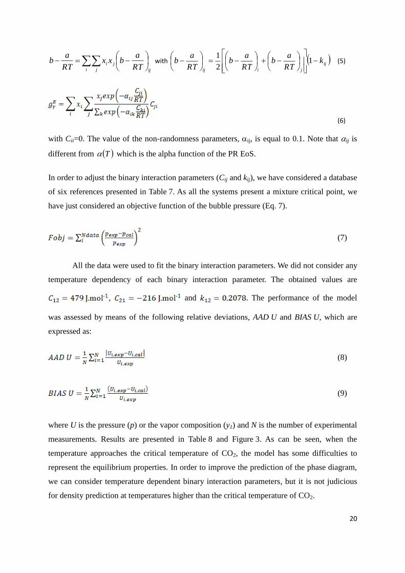
with Cii=0. The value of the non-randomness parameters, ij, is equal to 0.1. Note that ij is
different from T which is the alpha function of the PR EoS.
In order to adjust the binary interaction parameters (Cij and kij), we have considered a database
of six references presented in Table 7. As all the systems present a mixture critical point, we
have just considered an objective function of the bubble pressure (Eq. 7).
(7)
All the data were used to fit the binary interaction parameters. We did not consider any
temperature dependency of each binary interaction parameter. The obtained values are
, and . The performance of the model
was assessed by means of the following relative deviations, AAD U and BIAS U, which are
expressed as:
(8)
(9)
where U is the pressure (p) or the vapor composition (y1) and N is the number of experimental
measurements. Results are presented in Table 8 and Figure 3. As can be seen, when the
temperature approaches the critical temperature of CO2, the model has some difficulties to
represent the equilibrium properties. In order to improve the prediction of the phase diagram,
we can consider temperature dependent binary interaction parameters, but it is not judicious
for density prediction at temperatures higher than the critical temperature of CO2.

21
Table 7 : Summary of vapor liquid equilibrium data of the binary system CO2 + O2.
Reference Type of Data Temperatures
Fredenslund and Sather 197019
pTxy 263.15, 273.15 and 283.15
Kaminishi and Toriumi 196620
pTxy 253.15, 273.15, 288.15 and 298.15
Muirbrook and Prausnitz 196521
pTxy 273.15
Zenner and Dana 196322
pTxy 273.15
Lasala et al. 201623
pTxy 273.15, 288.15 and 298.15
Westman et al. 201624
pTxy 273.09 and 293.08
Table 8: Values of BIAS, and AAD of pressure and vapor compositions for the different sets of data.
Reference T/K BIAS p/% BIAS y/% AAD p/% AAD y/%
Fredenslund and Sather 197019
263.15 6.1 -1.6 6.1 2.5
273.15 4.8 -1.7 4.8 2.3
283.15 8.5 -3.7 8.5 3.7
Kaminishi and Toriumi 196620
253.15 6.9 -7.6 7.8 7.6
273.15 6.3 -4.4 6.3 4.4
288.15 5.6 -4.2 5.6 4.2
298.15 3.5 -2.0 3.5 2.0
Muirbrook and Prausnitz 196521 273.15 5.7 -1.8 5.7 3.4
Zenner and Dana 196322 273.15 4.6 -4.5 5.8 4.7
Lasala et al. 201623
273.15 12.6 -3.8 12.6 3.8
288.15 6.4 -2.8 6.4 2.8
298.15 Calculation failed close to mixture critical point
Westman et al. 201624
273.09 9.8 -3.3 9.8 3.9
293.08 2.1 -1.2 2.1 1.2

22
0
2
4
6
8
10
12
14
16
0.0 0.1 0.2 0.3 0.4 0.5 0.6
Pre
ssu
re /
MP
a
x1, y1
Figure 3 : Vapor – Liquid equilibrium isotherms for O2 (1) + CO2 (2) binary system: (Δ): 273.09 K from
Westman et al.24
, (o), 263.15 K from Fredenslund and Sather19
. Solid line: Peng Robinson EoS model,
Dashed line: EoS-CG (Gernert and Span8) EoS model.
PT envelopes of the three mixtures (see Table 2) are predicted using our thermodynamic
model and plotted in Figure 4. In this figure, we have also plotted the PT data of each system
corresponding to the measured densities. According to Figure 4, we can observe that few
density data were determined in the vapor-liquid region. Probably for these data, we are in a
metastable state (mixture 3, T=279.05 and 293.31 K, mixture 1, T=276.59 K). These data are
mentioned in Tables 3 and 5.

23
0
2
4
6
8
10
12
14
16
18
20
210 260 310 360 410
p /
MP
a
T /K(a)
0
2
4
6
8
10
12
14
16
18
20
210 260 310 360 410
p /
MP
a
T /K
(b)

24
0
2
4
6
8
10
12
14
16
18
20
210 260 310 360 410
p /
MP
a
T /K
(c)
Figure 4: Pressure Temperature envelope of the CO2-O2 binary system calculated using Peng Robinson EoS (compositions listed in Table 2) showing the experimental points
measured (). (a): Mixture 1, (b): mixture 2, (c): Mixture 3. Grey solid line: Pure CO2 vapor pressure. Bold dashed line: mixture critical points line.

25
3.2. Comparison with experimental density data
The PR EoS previously developed is used to predict the experimental data. Table 9
summarizes the AAD (Eq. 10) and Maximum Absolute Deviation (MAD) in the gas, liquid and
supercritical regions. The results (pressure vs. molar volume and compressibility factor) for
the different mixtures are presented in Figures 5 to 7.
(10)
As it can be seen, the cubic EoS represents the experimental data with satisfactory deviations.
As the compressibility factor tends to 1 when the pressure tends to 0 (ideal gas law), it is
possible to evaluate the second virial coefficient of the CO2 – O2 binary mixture from the
measured compressibility factor. Indeed, for low to moderate pressure. It is also a
good test to evaluate the consistency of the data at low pressure. In addition, we can observe
that the maximum of deviation occurs for the low-pressure measurements (p < 1.5 MPa due to
VTD precision) and close to bubble or dew points (possible metastable states). As the
compressibility depends on the temperature, the density and the pressure, the uncertainties of
the compressibility are therefore expressed using Eq. (11). It can be observed that the
compressibility factor “concentrates” all the uncertainties of the measurements. The average
value of u(Z)/Z is around 5%.
(11)

26
0
2
4
6
8
10
12
14
16
18
20
0 100 200 300 400 500 600 700 800 900
Pre
ssio
n /
MP
a
Masse volumique/ kg.m-3
0.3
0.4
0.5
0.6
0.7
0.8
0.9
1
1.1
0 5 10 15 20
Co
mp
ress
ibili
ty fa
cto
r /
Z
Pressure/ MPa
A B
Figure 5: A: Pressure as a function of molar density for the O2 + CO2 (mixture 1: 0.274/0.726) binary system. B: Compressibility factor as a function of pressure (Δ):
276.59 K, (×): 353.78 K, ():416.38 K. Solid line: Peng Robinson EoS with Wong Sandler mixing rules and NRTL Activity coefficient model.

27
0
2
4
6
8
10
12
14
16
18
20
0 100 200 300 400 500 600
Pre
ssu
re /
MP
a
Density/ kg.m-3
0.5
0.6
0.7
0.8
0.9
1
1.1
0 2 4 6 8 10 12 14 16 18 20
Co
mp
ress
ibili
ty fa
cto
r /
Z
Pressure/ MPa
A B
Figure 6: A: Pressure as a function of molar density for the O2 + CO2 (mixture 2: 0.483/0.517) binary system. B: Compressibility factor as a function of pressure (Δ):
280.63 K, (×): 353.46 K, ():412.85 K. Solid line: Peng Robinson EoS with Wong Sandler mixing rules and NRTL Activity coefficient model.

28
0
2
4
6
8
10
12
14
16
18
20
0 100 200 300 400 500 600 700 800 900 1000
Pres
sure
/ M
Pa
Density/ kg.m-3
0.1
0.2
0.3
0.4
0.5
0.6
0.7
0.8
0.9
1
1.1
0 5 10 15 20
Co
mp
ress
ibil
ity
fa
cto
r /
Z
Pressure/ MPa
A B

29
0
2
4
6
8
10
12
0 20 40 60 80 100 120 140 160 180 200P
ress
ure
/ M
Pa
Density/ kg.m-3
C
Figure 7: A: Pressure as a function of molar density for the O2 + CO2 (mixture 3: 0.128/0.872) binary system (C: zoom in the low pressure region). (Δ): this work.
(): Mantovani et al.7, (): Lozano-Martin et al.
5 B: Compressibility factor as a function of pressure (Δ): 279.05 K, (×): 353.62 K, ():414.31 K. Solid and dashed
line: Peng Robinson EoS with Wong Sandler mixing rules and NRTL Activity coefficient model.

30
A
B
Figure 8: A: Pressure as a function of density for the CO2 + O2 (mixture 1: 0.726/0.274) binary system. B: Compressibility factor as a function of pressure (Δ): 276.
50 K, (×): 353.78 K, (): 416.38 K. Solid line: EOS-CG.

31
A
B
Figure 9: A: Pressure as a function of density for the CO2 + O2 (mixture 2: 0.517/0.483) binary system. B: Compressibility factor as a function of pressure (Δ):
280.63 K, (×): 353.46 K, (): 412.85 K. Solid line: EOS-CG.

32
A
B

33
C
Figure 10: A: Pressure as a function of density for the CO2 + O2 (mixture 3: 0.872/0.128) binary system (C: zoom in the low pressure region). (Δ): this work. ():
Mantovani et al.7, (): Lozano-Martin et al.
5 B. B: Compressibility factor as a function of pressure (Δ): 279.05 K, (×): 353.62 K, (): 414.31 K. Solid line: EOS-CG.

34
Experimental density data were also compared to a recent EoS, EOS-CG, based on GERG-
20084, 15
. Parameters for the reduced mixture density and inverse reduced mixture temperature
are provided by Gernert and Span8, but the weighting factor Fij is set to 0 for the binary
system CO2-O2. As a result, the residual mixture behavior only includes the residual behavior
of the pure components, weighted by their molar fraction. The reducing functions for density
and temperature are presented in Eqs. (11) and (12), where N is the number of components,
TC,i is the critical temperature of component i and C,i is the critical density of component i.
(11)
(12)
, , and are binary interaction parameters from GERG-20084, 15
and
presented in Table 10 for the system CO2-O2.
As shown in Table 9, EoS-CG predicts the densities more accurately than the PR EoS
developed in this work. It should be noted that EOS-CG is based on multi-fluid
approximations and that different types of data (PT, VLE, speed of sound, etc.) are used for
the development of binary model parameters. Figures 8 - 10 compare experimental and
predicted densities and compressibility factors. Due to the use of different data types, rather
than only VLE as PR EoS, the phase equilibrium prediction is less accurate for EOS-CG than
for PR EoS (see Figure 3). This is also influenced by the presence of a mixture critical point.
Finally, we have compared our experimental results with literature data for compositions
similar to ours, i.e. mixture 3. We have plotted the literature data in Figures 7 and 10 (we have
also included a zoom to better visualize the low-pressure region). Deviations between these
data and PR EoS and EOS-CG are presented in Table 9. As can seen, the order of magnitude
of the deviations between our models and experimental data (and our data and literature data)
are very close. We can observe a good agreement between the different sets of data.

35
Table 9: Deviations between experimental and calculated data using Peng Robinson EoS with the Wong Sandler mixing rules involving NRTL activity coefficient
model, and using EoS-CG. Vap: vapor phase, Liq: liquid phase and SC: supercritical region.
Peng Robinson EoS EoS-CG
T/K AAD/% AAD/% AAD/% MAD% MAD% MAD% AAD/% AAD/% AAD/% MAD% MAD% MAD%
Vap Liq SC Vap Liq SC Vap Liq SC Vap Liq SC
Mixture 1
276.59 4.2 3.2
10.1 3.8
0.7 1.3 2.2 3.3
293.18
3.2
4.5 1.3 3.8
313.18
2.0
3.9 1.5 2.2
334.78
2.2
3.9 0.6 1.3
353.78
1.5
3.1 0.8 1.3
373.46
1.4
2.4 0.5 0.7
395.18
1.3
2.1 0.6 0.7
416.38
0.9
1.4 0.4 0.9
Mixture 2
280.63
2.8
4.6 1.6 3.7
293.92
2.7
4.7 2.1 3.4
313.63
3.1
4.4 2.1 2.8
333.21
1.4
2.4 0.8 1.4
353.46
1.6
2.4 1.0 1.6
373.60
1.5
2.2 1.3 1.9
395.72
1.9
4.7 1.7 2.3
412.85
1.1
2.8 0.7 1.2
Mixture 3
279.05 3.0 3.7
12.6 8.2
2.3 1.8 5.1 2.0
293.31
3.7
8.9 2.2 1.7 5.0 2.1
315.06
3.5
8.6 1.1 3.1
333.25
2.3
7.1 0.9 2.3
353.62
1.6
6.8 0.9 3.1

36
374.23
1.4
4.5 1.7 5.1
394.15
1.0
3.0 0.3 0.8
414.31
0.8
2.4 0.4 0.8
Lozano-Martín et al.5, xO2=0.099856 – Maximum pressure: 9 MPa
293.07 1.94 3.1 0.3 0.8
349.92 1.78 2.5 0.2 0.3
374.91 1.28 1.7 0.07 0.2
Mantovani et al.7, xO2=0.1291 – Maximum pressure: 20 MPa
303.22 3.86 9.96 5.1 13.6
323.18 3.57 6.29 4.0 6.5
343.15 3.34 7.55 3.4 7.1
363.15 3.02 8.20 3.0 7.8
383.14 3.76 15.18 3.6 14.8

37
Table 10: Values of EoS-CG4 binary interaction parameters.
System βT γT βv γv
CO2 + O2 1.0 1.032 1.0 1.0845
4. Conclusion
The densities of three CO2-O2 binary mixtures were measured using VTD densitometer,
Anton Paar DMA 512, in the gas, liquid and supercritical regions. The densitometer was first
calibrated using pure CO2 and the FPMC calibration technique. The maximum expanded
uncertainties on temperature, pressure and densities are U(p)= 0.0005 MPa, U(T)= 0.3 K and
U()= 15 kg.m-3
, respectively. The highest uncertainties were observed at very low pressure
conditions in the gas phase or in the vicinity of the bubble point curve in the liquid phase. The
measured densities were employed to evaluate the classical Peng-Robinson cubic EoS with
parameters adjusted on VLE data from the literature. The model gives satisfactory results in
the prediction of the volumetric properties in the typical conditions of storage in salt caverns.
However, the GERG-2008-based EoS-CG was more accurate with AAD of only 1.1% and
MAD of 5.1%. The main advantage of EOS based on a thermodynamic potential is that all
thermodynamic properties of a mixture or pure substance can be consistently derived from the
potential; these properties are needed in the assessment of cavern stability.
5. Acknowledgments
Financial support from Agence Nationale de la Recherche (ANR) through the project
FluidSTORY (n° 7747, ID ANR-15-CE06-0015) is gratefully acknowledged.
6. References
1. Götz, M.; Lefebvre, J.; Mörs, F.; Koch, A. M.; Graf, F.; Bajohr, S.; Reimert, R.; Kolb,
T., Renewable Power-to-Gas: A technological and economic review. Renewable energy 2016,
85, 1371-1390.

38
2. Kezibri, N.; Bouallou, C., Conceptual design and modelling of an industrial scale
power to gas-oxy-combustion power plant. Int. J. Hydrogen Energy 2017, 42, (30), 19411-
19419.
3. Blanco-Martín, L.; Rouabhi, A.; Hadj-Hassen, F., Use of salt cavern in the energy
transition context: application to the Power-to-Gas– Oxyfuel process. SN Appl. Sci. 2020,
submitted.
4. Li, H.; Dong, B.; Yu, Z.; Yan, J.; Zhu, K., Thermo-physical properties of CO2 mixtures
and their impacts on CO2 capture, transport and storage: progress since 2011. Appl. Energy
2019, 255, 113789.
5. Lozano-Martin, D.; Akubue, G.U.; Moreau, A.; Tuma, D.; Chamorro, C.R., Accurate
experipmental (p, , T) data of the (CO2+O2) binary system for the development of models
for CCs processes. J. Chem. Thermodyn. 2020, 150, 106210.
6. Commodore, J.A.; Deering, C.E.; Marriott, R.A., Volumetric properties and phase
behavior of sulfur dioxide, carbon disulfide and oxygen in high-pressure carbon dioxide fluid.
Fluid Phase Equilib. 2018, 477, 30-39.
7. Mantovani, M.; Chiesa, P.; Valenti, G.; Gatti, M.; Consonni, S., Supercritical pressure-
density-temperature measurements on CO2-N2, CO2-O2 and CO2-Ar binary mixtures. J.
Supercrit. Fluids 2012, 61-34-43.
8. Gernert, J.; Span, R., EOS–CG: A Helmholtz energy mixture model for humid gases
and CCS mixtures. J. Chem. Thermodyn. 2016, 93, 274-293.
9. Rivollet, F.; Jarne, C.; Richon, D., PρT and VLE for Ethane+ Hydrogen Sulfide from
(254.05 to 363.21) K at Pressures up to 20 MPa. J Chem. Eng. Data 2005, 50, (6), 1883-1890.
10. Coquelet, C.; Ramjugernath, D.; Madani, H.; Valtz, A.; Naidoo, P.; Meniai, A. H.,
Experimental measurement of vapor pressures and densities of pure hexafluoropropylene. J
Chem. Eng. Data 2010, 55, (6), 2093-2099.
11. Nazeri, M.; Chapoy, A.; Valtz, A.; Coquelet, C.; Tohidi, B., Densities and derived
thermophysical properties of the 0.9505 CO2+ 0.0495 H2S mixture from 273 K to 353 K and
pressures up to 41 MPa. Fluid Phase Equilib. 2016, 423, 156-171.
12. Bouchot, C.; Richon, D., An enhanced method to calibrate vibrating tube densimeters.
Fluid phase Equilib. 2001, 191, (1-2), 189-208.
13. Khalil, W.; Coquelet, C.; Richon, D., High-pressure Vapor− Liquid equilibria, liquid
densities, and excess molar volumes for the carbon dioxide+ 2-propanol system from (308.10
to 348.00) K. J. Chem. Eng. Data 2007, 52, (5), 2032-2040.
14. Lemmon, E.; Bell, I. H.; Huber, M.; McLinden, M., NIST Standard Reference
Database 23: Reference Fluid Thermodynamic and Transport Properties-REFPROP, Version
10.0, National Institute of Standards and Technology. 2018. URL http://www.nist.
gov/srd/nist23. cfm.
15. Span, R.; Wagner, W., A new equation of state for carbon dioxide covering the fluid
region from the triple‐point temperature to 1100 K at pressures up to 800 MPa. J. Phys. Chem.
Ref. Data 1996, 25, (6), 1509-1596.
16. Peng, D.-Y.; Robinson, D. B., A new two-constant equation of state. IEC Fund. 1976,
15, (1), 59-64.

39
17. Wong, D. S. H.; Sandler, S. I., A theoretically correct mixing rule for cubic equations
of state. AIChE J. 1992, 38, (5), 671-680.
18. Renon, H.; Prausnitz, J. M., Local compositions in thermodynamic excess functions
for liquid mixtures. AIChE J. 1968, 14, (1), 135-144.
19. Fredenslund, A.; Sather, G., Gas-liquid equilibrium of the oxygen-carbon dioxide
system. J. Chem. Eng. Data 1970, 15, (1), 17-22.
20. Kaminishi, G.-i.; Toriumi, T., Gas-liquid equilibrium under high pressures. VI. Vapor-
liquid phase equilibrium in the CO2-H2, CO2-N2, and CO2-O2 systems. Kogyo Kagaku
Zasshi 1966, 69, (2), 175-178.
21. Muirbrook, N.; Prausnitz, J., Multicomponent vapor‐liquid equilibria at high
pressures: Part I. Experimental study of the nitrogen—oxygen—carbon dioxide system at 0°
C. AIChE J. 1965, 11, (6), 1092-1096.
22. Zenner, G.H.; Dana, L.I Liquid-vapor equilibrium compositions of carbon dioxide-
oxygen-nitrogen mixtures, Chemical engineering progress symposium series, 1963, 36-41.
23. Lasala, S.; Chiesa, P.; Privat, R.; Jaubert, J.-N., VLE properties of CO2–Based binary
systems containing N2, O2 and Ar: Experimental measurements and modelling results with
advanced cubic equations of state. Fluid Phase Equilib. 2016, 428, 18-31.
24. Westman, S. F.; Stang, H. J.; Løvseth, S. W.; Austegard, A.; Snustad, I.; Ertesvåg, I. S.,
Vapor-liquid equilibrium data for the carbon dioxide and oxygen (CO2+ O2) system at the
temperatures 218, 233, 253, 273, 288 and 298 K and pressures up to 14 MPa. Fluid Phase
Equilib. 2016, 421, 67-87.

40
TOC GRAPHIC
Saltcavern
CO2
O2
MeasurementsData treatment / consistencyPhase diagram
Vibrating Tube Densitometer