August 2005

NASA/TM-2005-213783

Experiment to Characterize Aircraft Volatile

Aerosol and Trace-Species Emissions

(EXCAVATE)

B. E. Anderson, H.-S. Branham, C. H. Hudgins, and J. V. Plant

Langley Research Center, Hampton, Virginia

J. O. Ballenthin, T. M. Miller, and A. A. Viggiano

Air Force Research Laboratory, Hanscom AFB, Massachusetts

D. R. Blake, University of California at Irvine, Irvine, California

H. Boudries, M. Canagaratna, R. C. Miake-Lye, T. Onasch, J. Wormhoudt, and D. Worsnop

Aerodyne Research, Inc., Billerica, Massachusetts

K. E. Brunke, Christopher Newport University, Newport News, Virginia

S. Culler, P. Penko, and T. Sanders, Glen Research Center, Cleveland, Ohio

H.-S. Han, P. Lee, and D. Y. H. Pui, Univeristy of Minnesota, Minneapolis, Minnesota

K. L. Thornhill, Science Applications International Corporation, Hampton, Virginia

E. L. Winstead, GATS Inc., Hampton, Virginia

The NASA STI Program Office . . . in Profile

Since its founding, NASA has been dedicated to the

advancement of aeronautics and space science. The

NASA Scientific and Technical Information (STI)

Program Office plays a key part in helping NASA

maintain this important role.

The NASA STI Program Office is operated by

Langley Research Center, the lead center for NASA’s

scientific and technical information. The NASA STI

Program Office provides access to the NASA STI

Database, the largest collection of aeronautical and

space science STI in the world. The Program Office is

also NASA’s institutional mechanism for

disseminating the results of its research and

development activities. These results are published by

NASA in the NASA STI Report Series, which

includes the following report types:

• TECHNICAL PUBLICATION. Reports of

completed research or a major significant phase

of research that present the results of NASA

programs and include extensive data or

theoretical analysis. Includes compilations of

significant scientific and technical data and

information deemed to be of continuing

reference value. NASA counterpart of peer-

reviewed formal professional papers, but having

less stringent limitations on manuscript length

and extent of graphic presentations.

• TECHNICAL MEMORANDUM. Scientific

and technical findings that are preliminary or of

specialized interest, e.g., quick release reports,

working papers, and bibliographies that contain

minimal annotation. Does not contain extensive

analysis.

• CONTRACTOR REPORT. Scientific and

technical findings by NASA-sponsored

contractors and grantees.

• CONFERENCE PUBLICATION. Collected

papers from scientific and technical

conferences, symposia, seminars, or other

meetings sponsored or co-sponsored by NASA.

• SPECIAL PUBLICATION. Scientific,

technical, or historical information from NASA

programs, projects, and missions, often

concerned with subjects having substantial

public interest.

• TECHNICAL TRANSLATION. English-

language translations of foreign scientific and

technical material pertinent to NASA’s mission.

Specialized services that complement the STI

Program Office’s diverse offerings include creating

custom thesauri, building customized databases,

organizing and publishing research results ... even

providing videos.

For more information about the NASA STI Program

Office, see the following:

• Access the NASA STI Program Home Page at

http://www.sti.nasa.gov

• E-mail your question via the Internet to

help@sti.nasa.gov

• Fax your question to the NASA STI Help Desk

at (301) 621-0134

• Phone the NASA STI Help Desk at

(301) 621-0390

• Write to:

NASA STI Help Desk

NASA Center for AeroSpace Information

7121 Standard Drive

Hanover, MD 21076-1320

National Aeronautics and

Space Administration

Langley Research Center

Hampton, Virginia 23681-2199

August 2005

NASA/TM-2005-213783

Experiment to Characterize Aircraft Volatile

Aerosol and Trace-Species Emissions

(EXCAVATE)

B. E. Anderson, H.-S. Branham, C. H. Hudgins, and J. V. Plant

Langley Research Center, Hampton, Virginia

J. O. Ballenthin, T. M. Miller, and A. A. Viggiano

Air Force Research Laboratory, Hanscom AFB, Massachusetts

D. R. Blake, University of California at Irvine, Irvine, California

H. Boudries, M. Canagaratna, R. C. Miake-Lye, T. Onasch, J. Wormhoudt, and D. Worsnop

Aerodyne Research, Inc., Billerica, Massachusetts

K. E. Brunke, Christopher Newport University, Newport News, Virginia

S. Culler, P. Penko, and T. Sanders, Glen Research Center, Cleveland, Ohio

H.-S. Han, P. Lee, and D. Y. H. Pui, Univeristy of Minnesota, Minneapolis, Minnesota

K. L. Thornhill, Science Applications International Corporation, Hampton, Virginia

E. L. Winstead, GATS Inc., Hampton, Virginia

Available from:

NASA Center for AeroSpace Information (CASI) National Technical Information Service (NTIS)

7121 Standard Drive 5285 Port Royal Road

Hanover, MD 21076-1320 Springfield, VA 22161-2171

(301) 621-0390 (703) 605-6000

The use of trademarks or names of manufacturers in the report is for accurate reporting and does not

constitute an official endorsement, either expressed or implied, of such products or manufacturers by the

National Aeronautics and Space Administration.

iii

Contents

1.0. Project Summary ...........................................................1

2.0. Introduction ...............................................................2

3.0. Experiment................................................................5

3.1. Facilities and Aircraft Engines .............................................5

3.2. Sample Probes and Systems ...............................................5

3.3. Measurements..........................................................6

3.4. Fuels .................................................................8

3.5. Experiment Matrices.....................................................8

4.0. Summary of Results.........................................................9

4.1. Engine Operating Parameters and Exhaust Properties ...........................9

4.2. Tracers and Hydrocarbons ...............................................10

4.3. Gas-Phase HOHO and SOx Species ........................................10

4.4. Particulate Physical Properties ............................................10

4.5. Particle Composition ...................................................11

4.6. Ion Density and Chemi-ion Speciation......................................11

5.0. References ...............................................................11

Tables ......................................................................12

Figures......................................................................20

Appendix A—Performance Evaluation of Particle Sampling Probes for Emission

Measurements of Aircraft Jet Engines..........................................29

Appendix B—Hydrocarbon Emissions from a Modern Commercial Airliner...............33

Appendix C—Technical Support of Measurements of SO2, SO3, HONO, CO2 .............50

Appendix D—Concentrations and Physical Properties of Jet Engine Exhaust

Aerosols Sampled during EXCAVATE ........................................60

Appendix E—Improved Nanometer Aerosol Size Analyzer ............................96

Appendix F—Real Time Characterization of Aircraft Particulate Emission by

an Aerosol Mass Spectrometer During EXCAVATE 2002 ........................124

Appendix G—AFRL Report on the NASA EXCAVATE Project.......................139

Appendix H—Particle Size Distributions Measured in B757 Engine Plume

During EXCAVATE ......................................................151

iv

1.0. Project Summary

The Experiment to Characterize Aircraft Volatile and Trace Species Emissions

(EXCAVATE) was conducted at Langley Research Center (LaRC) in January 2002 and focused

upon assaying the production of aerosols and aerosol precursors by a modern commercial

aircraft, the Langley B757, during ground-based operation. Remaining uncertainty in the post-

combustion fate of jet fuel sulfur contaminants, the need for data to test new theories of particle

formation and growth within engine exhaust plumes, and the need for observations to develop air

quality models for predicting pollution levels in airport terminal areas were the primary factors

motivating the experiment. NASA’s Atmospheric Effects of Aviation Project (AEAP) and the

Ultra Effect Engine Technology (UEET) Program sponsored the experiment which had the

specific objectives of determining ion densities; the fraction of fuel S converted from S(IV) to

S(VI); the concentration and speciation of volatile aerosols and black carbon; and gas-phase

concentrations of long-chain hydrocarbon and PAH species, all as functions of engine power,

fuel composition, and plume age.

Participants in EXCAVATE were solicited from among groups funded by AEAP and UEET

to characterize engine emissions and near-field interactions and included: the tunable diode laser

(TDL) and aerosol mass spectrometers (AMS) teams from Aerodyne Research, Inc.; the Particle

and Gaseous Emissions Measurement System (PAGEMS) from NASA Glenn Research Center

(GRC); the electron impact (EIMS) and chemical ionization mass spectrometer (CIMS) group

from the Air Force Research Laboratory (AFRL); the nano-aerosol size analyzer (nASA) team

from the University of Minnesota (UM); the whole air sampling group from the University of

California at Irvine (UCI); and the in situ measurements group from NASA LaRC. Parameters

and species that were measured included exhaust gas velocity, temperature, and CO2

concentration; engine pressure ratios/power settings, fan speeds, combustor temperatures, and

fuel-flow rates; sample stream CO2, SO2, SO3, H2SO4, HONO, HNO3, nonmethane hydro-

carbons, and halocarbons; aerosol number densities and size distributions as a function of sample

temperature; and aerosol mass and composition. Using well-characterized gas and aerosol probes

and measurement systems, the participants collected data behind both the Langley T-38A

(J85-GE engine) and B-757 (RB211) aircraft at sampling distances ranging from 1 to 35 m. For

the B-757, fuels containing 810, 1050, and 1820 ppm S were burned in the tests to evaluate the

impact of fuel S upon particle densities in the exhaust plume, and data were collected over a

range of power settings from idle to near takeoff thrust. In the case of the T-38, a single fuel was

burned (810 ppm), but data were collected over a variety of aerosol dilutions to evaluate the role

of sampling techniques upon aerosol number densities and size distributions.

The following text, tables, and graphs provide detailed information regarding the aircraft

operating parameters and engine emission characteristics. Important conclusions that one can

draw from EXCAVATE observations include:

• Chem-ion densities were very high in the exhaust of both aircraft and are consistent with

values that are presently being used in microphysical models of aerosol formation inexhaust plumes.

• Both aircraft emit high concentrations of organic aerosols at low power settings.

2

• At idle, the aircraft emit much higher levels of organic aerosols than black carbon

particles.

• Black carbon emission indices increase significantly in going from idle to cruise power.

• Observed aerosol size distributions were highly dependent upon the sample dilution ratio.

• Higher than expected levels of HONO were observed in the B757 exhaust.

• Total particle emission indices were typically a factor of 10 higher at 25 to 35 m than at 1

m downstream of the exhaust plane, indicating that significant numbers of new particles

form within the exhaust plume as it cools and dilutes.

• The concentration of sulfate aerosol increased considerably as sampling took place

progressively further downstream of the exhaust plane, suggesting that sulfate particles

form and undergo rapid growth within aircraft exhaust plumes.

• Emission indices for sulfate aerosols were directly dependent on the fuel sulfur

concentration and typically represented 0.5 percent of the total sulfur budget.

• Aerosol concentrations and characteristics take several minutes to reach equilibrium

values after changes in engine power. This was particularly notable when one reduced

the engines from high to low power, a situation found during the aircraft landing cycle. In

this case, the engines produced high concentrations of large organic aerosol particles for

several minutes after power was reduced from a cruise setting to idle.

2.0. Introduction

Because of concern that aviation-related emissions may detrimentally impact the atmospheric

environment, NASA initiated a major research effort-AEAP-aimed at characterizing the impact of

current and future fleets of commercial aircraft on atmospheric chemical and radiative processes.

To pursue this goal, the AEAP funded investigators to explore a wide range of topics, from

determining what pollutants are formed within specific combustors to examining how the

integrated emissions from the aircraft fleet influence ozone chemistry and cloud coverage.

In order to manage and assimilate information from these diverse topic areas, the AEAP was

organized into six interacting subelements, each charged with specific goals and tasks. For

example, the “Emission Scenarios” element gathers statistics on current and projected flight routes,

the aircraft fleet, and the geographically distributed fuel use and pollutant production by aircraft

(i.e., Baughcum et al., 1998). In turn, investigators funded under the “Global Modeling” element

assimilate the emission scenario information into two-dimensional (2-D) and three dimensional

(3-D) models to assess the impact of the emissions upon global trace chemical budgets and climate.

The two subelements of AEAP addressed by EXCAVATE were “Engine Emission

Characterization” and “Near-Field Interactions,” which focus upon characterizing and quantifying

the direct particulate and gas-phase emissions of aircraft and determining how these exhaust

emissions are influenced by interaction with the atmosphere and the aircraft’s trailing wingtip

vortices. This paper describes a coordinated field experiment sponsored by these two subgroups to

3

characterize the speciation of sulfur and evolution of volatile aerosol particles in the exhaust from

the turbine engine of a typical commercial airliner.

The task of characterizing aircraft exhaust emissions was initially scoped at obtaining in-flight

verification of the test stand trace-gas emission index (EI) measurements and more quantitative data

on the level and properties of particulate matter produced by the engines. The primary species of

concern were reactive nitrogen compounds due to their role in regulating atmospheric O3 and soot

due to its ability to absorb solar radiation and its possible role in altering cloud microphysical

properties.

A large base of turbine engine emission data was already available from the manufacturers

because test stand measurements are required of all engines entering the commercial fleet. These

tests consist of quantifying the amount of NOx, CO, and unburned hydrocarbons emitted relative to

fuel burned as a function of thrust. They also include a determination of “smoke number,” a

parameter roughly equivalent to the amount of soot an engine generates. Computational models

were available to extrapolate the test stand EI data to cruise altitude conditions (Baughcum et al.,

1996). Early in-flight observations indicated that values for NOx derived in this manner were

accurate at least to within experimental uncertainty and that wake or plume processing did not

appreciably alter the expected EIs over time (Zheng et al., 1994; Fahey et al., 1995). It was thus

assumed reasonable to adopt the test stand EI data along with fleet and fuel burn statistics and

proceed with using 3-D models to evaluate the impact of aircraft NOx on the global ozone budget

(Friedl, 1997).

Characterizing the aerosol emissions from aircraft has proven to be a difficult task.

Particulates directly emitted by jet aircraft are mostly soot with traces of metals and heavy

unburned hydrocarbons. The smoke number data provided by manufacturers are only a

qualitative estimate of soot emission, dependent on sampling conditions and soot characteristics

and morphology, and of little value for estimating atmospheric impacts. Thus, new and more

detailed studies were required. Subsequent exhaust exit-plane measurements on engines

mounted in test cells and aircraft in runup facilities indicated that jet turbines produce on the

order of 1015

soot particles with a mean mass diameter of 40 to 60 nm per kg of fuel burned.

Hydration tests on the particles suggested they contain an appreciable amount of soluble material

(Hagen et al., 1992). This result was not surprising because aviation fuel contains, as an

impurity, varying amounts of sulfur (up to 3000 ppm), a fraction of which is oxidized during

combustion to form H2SO4, which can, in turn, be adsorbed onto the soot particles to improve

their hydration properties (Wyslouzil et al., 1994).

The AEAP sponsored in-flight measurements verified that aircraft are prodigious sources of

soot particles but yielded the surprising observation that they also produce an enormous number

of ultrafine volatile particles (Fahey, 1995). Assuming the particles were composed of sulfur

species, the results suggested that a significant fraction of the sulfur contaminants in jet fuel is

converted to S(VI) species either within the engine or very early in the exhaust plume evolution.

High S(IV) to S(VI) conversion efficiencies in aircraft engines and rapid formation of sulfuric

acid particles in aircraft plumes could have serious climatic implications as such particles play a

significant role in heterogeneous chemical processes (i.e., ozone destruction) as well as in

regulating cloud formation, duration, and radiative characteristics. The inferred amount of sulfate

observed in the experiment was inconsistent with the sulfate being produced by hydroxyl radical

(OH) oxidation alone and challenged the contemporary understanding of turbine engine chemical

kinetics.

4

The observations of volatile particles in aircraft plumes and the recognition of their potential

impact on atmospheric processes spurred a number of investigations to determine the fate of jet

fuel sulfur contaminants. Because it is exceedingly difficult to capture sufficient particulate

samples for quantitative analysis, these experiments took the approach of varying fuel S

concentrations and observing the corresponding impact upon bulk aerosol production and

characteristics. In the first of these tests, Busen and Schumman (1995) observed no visible

difference in the contrails from an aircraft with one engine burning 2 ppm S fuel and the other

aircraft burning 250 ppm S fuel. Subsequently, Schumman et al., (1996) found only a 25 percent

difference in ultrafine (>7 nm in diameter) particle concentrations in the near-field exhaust of

engines burning 170 and 5500 ppm S fuel. Later Miake-Lye et al. (1998) showed a direct

correlation between fuel sulfur content and aircraft production of volatile particles and estimated

an S(IV) to S(VI) conversion efficiency of 6 to 30% for a modern B757 airliner. In contrast,

Schumman et al. (2002) more recently estimated a conversion efficiency of <1 percent for an

ATTAS aircraft from observations of particulate and gas-phase H2SO4.

The lack of consensus in the experimental results coupled with the scarcity of data available

to validate and stimulate the development of engine and exhaust plume models clearly

established a need for more detailed and systematic studies of fuel S oxidation and aerosol

production by aircraft engines. Thus, in 1997 the AEAP “Emission Characterization” and

“Near-Field Interactions” groups developed collaborative experiments to sample the aerosol and

aerosol precursor emissions of a specific turbine engine, both under carefully controlled test

conditions and at cruise altitudes in varying environmental conditions. The engine tested was a

Pratt & Whitney Model F100 series 200E of the type used on U.S. Air Force F-16 and F-15

fighter jet aircraft. The experiments included a ground-based measurement program conducted

at the NASA Lewis Research Center Propulsion System Laboratory (Wey et al., 1998) and an

airborne campaign based at NASA Wallops Flight Facility to sample the near-field emissions

from U.S. Air National Guard F-16 aircraft (Anderson et al., 1999). Both venues included

extensive characterization of the engine emissions-including measurements of aerosol size and

volatility as well as gas-phase sulfur speciation-as functions of fuel sulfur, engine power, and

ambient altitude. Results of the airborne study suggest that for the F100 engine, volatile aerosol

production is highly dependent on fuel S concentration with observations being consistent with a

maximum of 3 percent of the Fuel S being converted from S(IV) to S(VI) in the near-field

wake. The ground-based tests gained insight into soot production and trace gas emissions as a

function of engine temperature and operating pressure, but line losses in the necessarily long

sampling tubes thwarted simultaneous attempts to measure SO3 and H2SO4-the primary forms of

S(VI) in the exhaust plume-to determine fuel S conversion efficiency.

Although the F100 engine tests and other experiments conducted by Europeans (Schumann et

al., 2002) added to a body of information suggesting that fuel S conversion factors were more

typically a few rather than tens of a percent, detailed information on precursor concentrations as

well as the formation, evolution, and composition of volatile aerosol particles in the exhaust of

commercial aircraft engines were still lacking. Thus, the AEAP in conjunction with the

environmental effects component of NASA’s UEET program sponsored EXCAVATE. A

ground-based study conducted in an open-air facility, EXCAVATE had the objective of

determining the concentration of chemi-ions; volatile aerosols and aerosol precursors; black

carbon; and selected gas-phase species within the exhaust plume of a modern commercial

turbofan engine as a function of engine power, fuel composition, and plume age. The

experiment took advantage of recent advances in instrumentation and paid particular attention to

5

determining time-dependent aerosol composition as well as chemi-ion speciation. Significant

efforts were made to minimize sample line lengths, characterize probe penetration efficiencies

and transmission losses, and evaluate the impact of sampling strategies upon measured

parameters. The paragraph below provides additional experimental details, summary results, and

appendices reporting the specific observation from each participating group.

3.0. Experiment

3.1. Facilities and Aircraft Engines

EXCAVATE took place during January 2000 at NASA LaRC. Emissions from two aircraft

were sampled during the mission: the NASA Langley Boeing 757 (B-757) and T-38A Talon.

The B-757 is a dedicated research aircraft that was obtained by NASA from Eastern Airlines and

has a relatively low number of hours on its engines and airframe. It is powered by a pair of Rolls

Royce, RB-211-535E4 turbofan engines, as are 80 percent of all B-757s in service. These

three-shaft, high bypass ratio engines produce 40100 lbs of thrust and have a single-stage wide-

chord fan, six-stage IP compressor, six-stage HP compressor, single annular combustor, single-

stage HP turbine, single-stage IP turbine, and a three-stage LP turbine. Langley’s T-38A is

powered by a pair of J85-GE-5A turbojet engines that produce 3850 lbs of thrust. Both aircraft

nominally burn commercial Jet A or military JP-5 fuels.

The engine tests were conducted at NASA’s “runup” facility that is located adjacent to a

heavily wooded area on the west side of the Langley Air Force Base (see fig. 1).

Basically a large concrete pad, the facility includes a blast fence that deflects the engine

exhaust upward to prevent damage to the neighboring vegetation. Water and electric power

outlets located on either side of the pad were used for cooling instruments and providing power

to experimenter equipment, respectively. Bolt holes and anchors are embedded at numerous

places in the pad to provide restraining points for aircraft during high power engine runs and

were used to secure the sampling probe sled and sample/electric lines to prevent them from being

blown back by the exhaust blast.

During tests, the aircraft were parked on a line extending out from the center of the blast fence

and chocked in place to keep them stationary during the high power engine runs. The sampling

sled was positioned behind the engine so that the tips of the sampling probes were 1 m down

steam and on the centerline of the turbine exhaust. For the B757, an additional aerosol-sampling

probe was affixed to the blast fence 25 m downstream of the engine exhaust plane. To obtain

aerosol samples at 10 and 35 m, the aircraft were rolled forward 9 m and rechocked. In the case

of the T-38A, additional aerosol inlets were mounted on weighted stands positioned 10 and 25 m

behind the engine exhaust plane; gas phase measurements were acquired only at 1-m separation

distance.

3.2. Sample Probes and Systems

Figures 2 and 3 show a photograph and a diagram, respectively, of the gas and primary

aerosol sampling probes that were designed by Robert Heirs from Arnold Engineering

Development Center for use in EXCAVATE. The aerosol probe was designed to introduce

a concentric flow of dilution gas as close behind the nozzle tip as possible to reduce particle

6

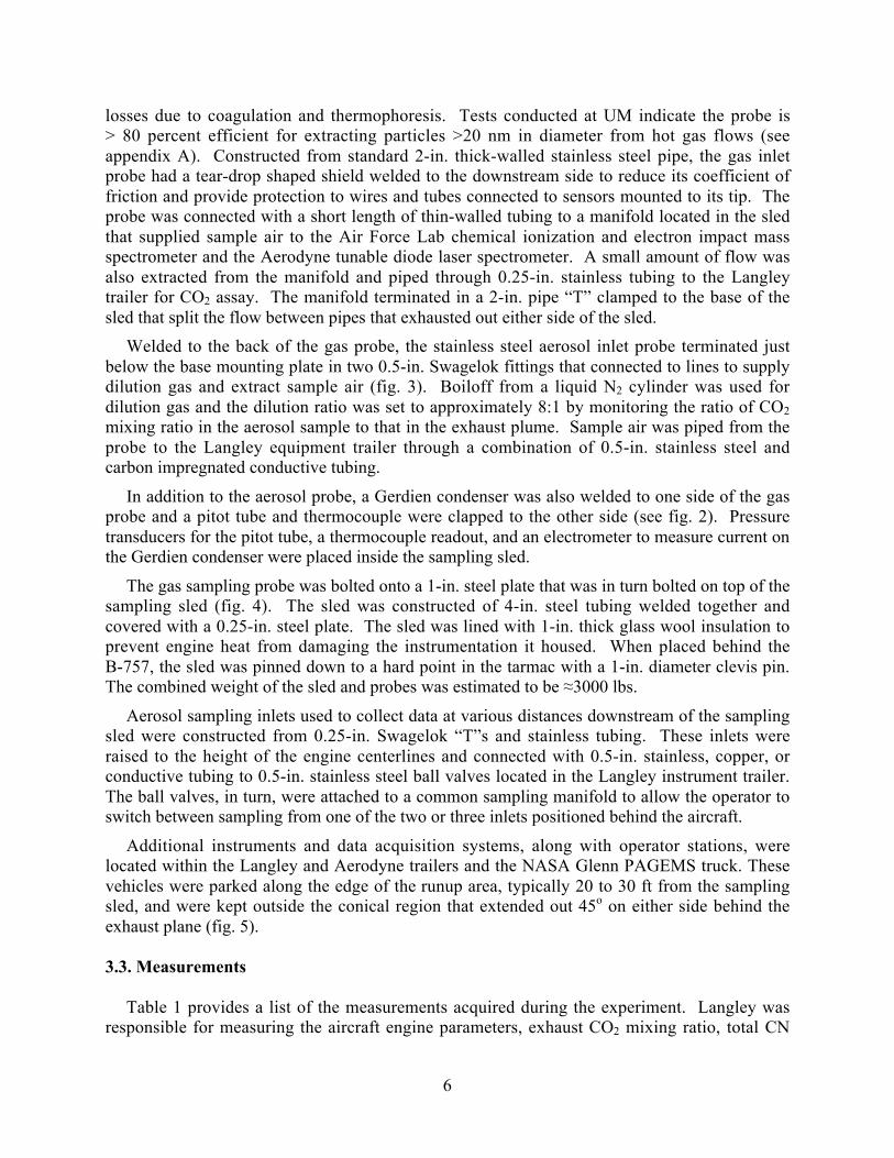
losses due to coagulation and thermophoresis. Tests conducted at UM indicate the probe is

> 80 percent efficient for extracting particles >20 nm in diameter from hot gas flows (see

appendix A). Constructed from standard 2-in. thick-walled stainless steel pipe, the gas inlet

probe had a tear-drop shaped shield welded to the downstream side to reduce its coefficient of

friction and provide protection to wires and tubes connected to sensors mounted to its tip. The

probe was connected with a short length of thin-walled tubing to a manifold located in the sled

that supplied sample air to the Air Force Lab chemical ionization and electron impact mass

spectrometer and the Aerodyne tunable diode laser spectrometer. A small amount of flow was

also extracted from the manifold and piped through 0.25-in. stainless tubing to the Langley

trailer for CO2 assay. The manifold terminated in a 2-in. pipe “T” clamped to the base of the

sled that split the flow between pipes that exhausted out either side of the sled.

Welded to the back of the gas probe, the stainless steel aerosol inlet probe terminated just

below the base mounting plate in two 0.5-in. Swagelok fittings that connected to lines to supply

dilution gas and extract sample air (fig. 3). Boiloff from a liquid N2 cylinder was used for

dilution gas and the dilution ratio was set to approximately 8:1 by monitoring the ratio of CO2

mixing ratio in the aerosol sample to that in the exhaust plume. Sample air was piped from the

probe to the Langley equipment trailer through a combination of 0.5-in. stainless steel and

carbon impregnated conductive tubing.

In addition to the aerosol probe, a Gerdien condenser was also welded to one side of the gas

probe and a pitot tube and thermocouple were clapped to the other side (see fig. 2). Pressure

transducers for the pitot tube, a thermocouple readout, and an electrometer to measure current on

the Gerdien condenser were placed inside the sampling sled.

The gas sampling probe was bolted onto a 1-in. steel plate that was in turn bolted on top of the

sampling sled (fig. 4). The sled was constructed of 4-in. steel tubing welded together and

covered with a 0.25-in. steel plate. The sled was lined with 1-in. thick glass wool insulation to

prevent engine heat from damaging the instrumentation it housed. When placed behind the

B-757, the sled was pinned down to a hard point in the tarmac with a 1-in. diameter clevis pin.

The combined weight of the sled and probes was estimated to be 3000 lbs.

Aerosol sampling inlets used to collect data at various distances downstream of the sampling

sled were constructed from 0.25-in. Swagelok “T”s and stainless tubing. These inlets were

raised to the height of the engine centerlines and connected with 0.5-in. stainless, copper, or

conductive tubing to 0.5-in. stainless steel ball valves located in the Langley instrument trailer.

The ball valves, in turn, were attached to a common sampling manifold to allow the operator to

switch between sampling from one of the two or three inlets positioned behind the aircraft.

Additional instruments and data acquisition systems, along with operator stations, were

located within the Langley and Aerodyne trailers and the NASA Glenn PAGEMS truck. These

vehicles were parked along the edge of the runup area, typically 20 to 30 ft from the sampling

sled, and were kept outside the conical region that extended out 45o on either side behind the

exhaust plane (fig. 5).

3.3. Measurements

Table 1 provides a list of the measurements acquired during the experiment. Langley was

responsible for measuring the aircraft engine parameters, exhaust CO2 mixing ratio, total CN

7

concentrations, black carbon, and submicron aerosol size distributions (see appendix B).

Aerodyne Research, Inc., made measurements of aerosol composition, using their new aerosol

mass spectrometer (appendix C), as well as operated the NASA GRC tunable diode laser system

that determined mixing ratios of CO2, SO2, SO3, and HONO (see appendix D). UM provided

nucleation mode size distributions for heated and unheated samples using their rapid scanning,

nASA (appendix E). AFRL provided a chemical ionization mass spectrometer, a Gerdien tube

condenser, and an ion mass spectrometer to measure a variety of species including SO2, H2SO4,

HNO3, total ion densities, and ion speciation (appendix F) and NASA GRC participated with

their PAGEMS van to make comparative measurements of aerosols and trace gases to evaluate

the status of their measurement systems and techniques with that of other participating groups.

Table 1. Measurements

Species/Parameter Technique Group

Engine parameters Aircraft systems LaRC

Fuel sulfur content X-ray fluorescence LaRC

Exhaust parameters (T, P, velocity) Pitot tubes, thermocouples LaRC

Sample and exhaust CO2 IR spectrometer LaRC

Aerosol size and volatility

(3 to 100 nm)

Nano differential mobility

analyzer (DMA)UM

Aerosol size (10 to 1000 nm) DMA, OPC LaRC & GRC

Black carbon Aethelometer LaRC

Nonmethane hydrocarbons Grab samples LaRC/UCI

SO2, CO2, SO3, H2O, HONO TDL Aerodyne/GRC

Aerosol composition Mass Spectrometer Aerodyne

H2SO4, HONO, HNO3, SO2 Chemical ion mass spectrometer AFRL

Ion density Gerdien condenser AFRL

Ion composition Ion Mass Spectrometer AFRL

LaRC: Langley Research Center, Bruce Anderson, PI

UCI: University of California, Don Blake, PI

UM: University of Minnesota, David Pui, PI

GRC: Glenn Research Center, Paul Penko and Clarence Change, PIs

Aerodyne MS group: Doug Worsnop, PI

Aerodyne TDL group: Joda Wormhoudt and Rick Miake-Lye, PIs

8

3.4. Fuels

EXCAVATE’s primary objectives included determining the post-combustion fate of fuel S

species and examining the formation and evolution of sulfur particles in the exhaust plume as a

function of engine power and plume age. To meet these objectives required burning fuels

of known and varying S concentrations. Although we had originally planned to obtain a low

S Jet-A fuel (<5ppm) and produce a medium (i.e., 100 ppm) and high S (1000 ppm) fuels from it

by adding tetrahydrothiophene, time and funding constraints forced us to purchase a JP-5 fuel

from the local government contractor and to produce a single, higher S content fuel by mixing in

tetrahydrothiophene sufficient to boost the S level by 1000 ppm. We thus ended with two fuels

from a single hydrocarbon matrix containing 1050+100 and 1820+100 ppm S for use in the

B-757 fuel S tests. A third JP-5 fuel obtained from the NASA Langley stock and containing

810+100 ppm S was used in the T-38A runs and in a B-757 experiment to test the sampling

system and to fill the role of low S fuel when the supply of 1050 ppm S fuel was depleted. Fuel

samples were sent to an independent testing laboratory where sulfur concentrations were

determined using X-ray fluorescence techniques.

3.5. Experiment Matrices

As discussed above, exhaust plumes from both the Langley T-38A and B-757 were sampled

during EXCAVATE, with the primary interest in sampling the T-38A being to test and perfect

our measurement procedures, determine optimum dilution ratios, and to evaluate sampling losses

as well as to obtain information on particle growth as the exhaust plume cools and disperses.

Varying engine power, sample dilution ratio, and sampling distance satisfied these objectives.

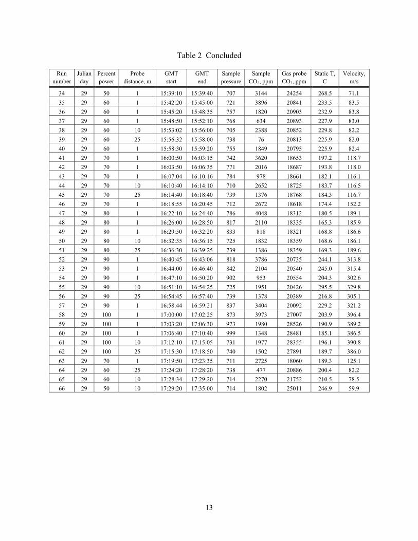
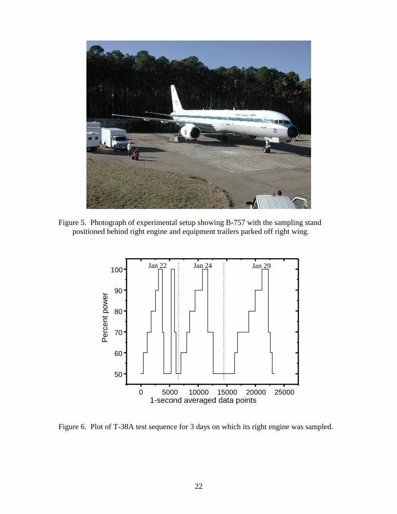
Table 2 lists the dates, times, duration, and test variable settings for the T-38A runs. Figure 6

provides a plot of the T-38A test matrix as a function of time at each setting. Data were recorded

on three different days (January 22, 24, and 29, 2002) at 10 percent power increments over

|the range from idle (50 percent) to full military power (100 percent of maximum rpm). On

January 29, data were collected from the 1-m probe using dilution ratios of approximately 8:1,

16:1, and 32:1 to test dilution effects and from additional probes located at 10 and 25 m to

observe the formation and growth of volatile aerosols as the plume aged and dispersed.

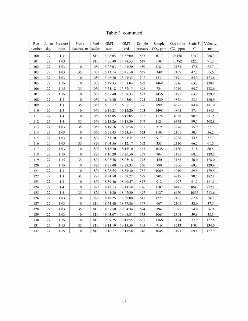
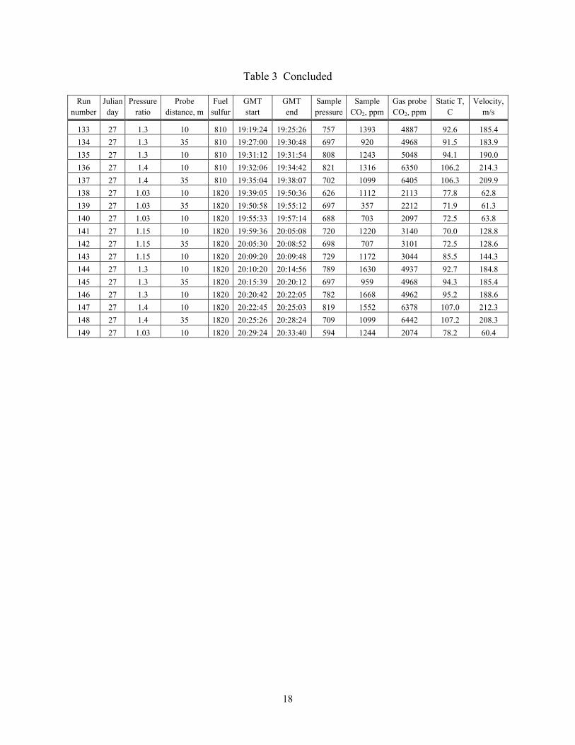
Table 3 lists the dates, times, duration and test variable settings for the B-757 runs. Figure 7

provides a plot of the B-757 test matrix as a function of time at each particular setting. Our

objectives in sampling this aircraft included determining the influence of fuel S on particle

formation; thus, test variables included engine power, sampling distance, and three different

levels of fuel S content. Based on results from the T-38A tests, dilution ratios were, where

possible, maintained at >8:1. Tests conducted on January 25 were to check instrument

functionality and to establish the range of engine power settings that the sampling rig could

withstand, so the full set of measurements was not recorded during these runs. Based on these

tests, we decided to collect data engine pressure ratios (EPRs) of 1.03 (idle), 1.15, 1.3, 1.4, and

1.5 when the probe was positioned at 1-m and to a maximum of 1.4 EPR when the probe was

positioned 10 m behind the engine. The 1.5 EPR is less than takeoff power (typically 1.6 to 1.7),

but was the highest power consistently achieved without overstressing the sampling stand and

instrument operators. On January 26, the primary inlet probes were positioned at 1 m and the

secondary aerosol inlet 25 m downstream. After a set of tests on the morning of January 27 to

evaluate the effect of sample dilution and cold engine starting on aerosol emission properties, the

9

aircraft was rolled forward 9 m and sets of data were acquired with a primary probe separation of

10 m and the secondary inlet at 35-m.

4.0. Summary of Results

4.1. Engine Operating Parameters and Exhaust Properties

Engine operating parameters and exhaust plume characteristics were recorded to facilitate

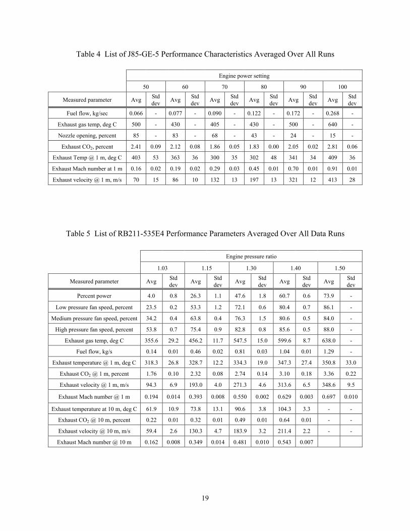
interpretation of simultaneous trace species measurements. Table 4 presents such data for the

J85-GE engine as observed during the T-38A test runs. The aircraft operator visually averaged

from cockpit indicators fuel-flow rate, exhaust gas temperatures at the combustor exit, and

nozzle openings and recorded the information in a logbook. A LiCor instrument measured CO2

fractions from exhaust gas samples collected 1-m downstream and on the centerline of the engine

exhaust plane. We derived exhaust gas temperatures and Mach numbers 1-m downstream of the

engine exhaust from total temperature and pressure measurements recorded from a thermocouple

and pitot-static sensor, respectively. Values for each parameter are given at six power settings,

ranging from idle (50 percent) to takeoff (100 percent). Not many of the plume thermodynamic

parameters exhibited 10 to 15 percent variability at any given power setting. Our measurements

for this study and those of others suggest that the engine requires several minutes to come to

thermal equilibrium after power changes. However, the thermocouple used during EXCAVATE

was very noisy, which may have exacerbated the problem.

Figure 8 shows how the fuel flow rate varies across the engine power range. At idle

(50 percent), the engine consumes 0.07 kg s-1

, whereas at takeoff or “full-military-power”

(100 percent), it burns about four times that amount. Assuming near 100 percent combustion

efficiency, the fuel:air ratio for the engine appears to reach a minimum at medium, or cruise,

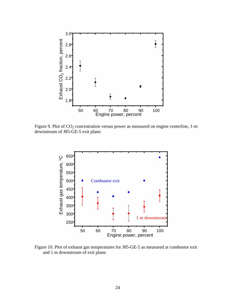
power settings ( 80percent; see fig. 9). Combustor exit temperature is also a minimum at cruise

power (fig. 10) and is positively correlated with exhaust CO2 fraction (fig. 9), which is

reasonable since both the temperature and CO2 mixing ratio are dependent on the amount of

ambient bypass air drawn through the engine in excess of that required for stoichiometric

combustion. Temperatures recorded 1 m downstream of the engine exit plane were typically 100

to 200 oC lower than at the combustor exit as a result of both mixing with bypass air and

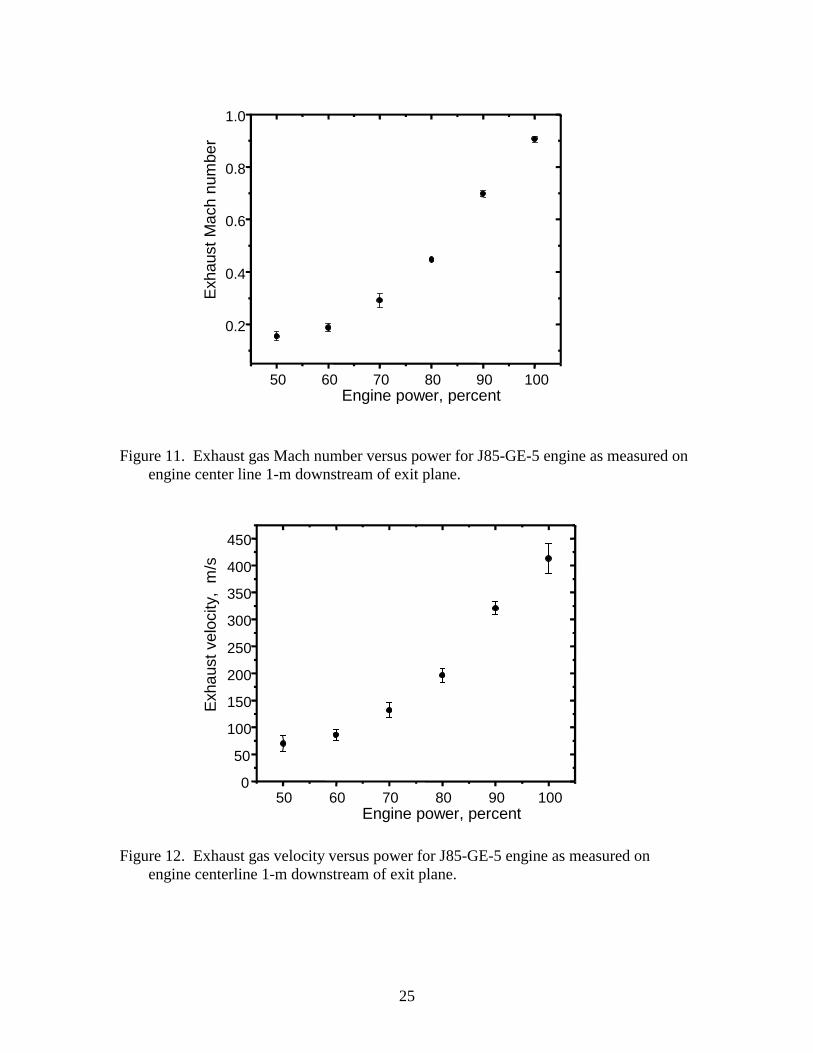
radiational cooling (fig. 10). The Mach number at the core of the exhaust plume 1-m

downstream of the engine exit plane varied from 0.16 to >0.9 on going from idle to 100 percent

power (fig. 11), which corresponds to velocities of 70 to over 410 m s-1

(fig. 12).

Table 5 shows the performance data for the RB-211-535E4 engine as observed during the

B-757 test runs. As for the T-38A, the aircraft operator visually averaged fuel-flow

rates, exhaust gas temperatures at the combustor exit, and fan speeds from cockpit indicators

and recorded them in a logbook. We determined the percentage power by comparing

the measured fuel-flow rates for each EPR with those listed for the various power

settings tested and archived by the International Civil Aviation Organization (ICAO:

<http://www.qinetiq.com/aircraft/aviation.html>). Again, we measured CO2 fractions by a

LiCor instrument from exhaust gas samples collected 1-m downstream and on the centerline of

the engine exhaust plane and exhaust gas temperatures, and derived Mach numbers 1-m

downstream of the engine exhaust from total temperature and pressure measurements recorded

from a thermocouple and pitot-static sensor, respectively. Values for each parameter are given at

10

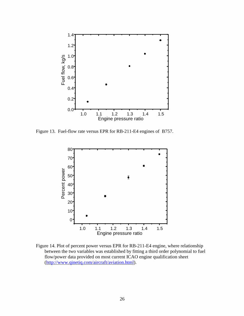
EPRs of 1.03 (idle), 1.15, 1.30, 1.40, and 1.50. EPR and engine power increase approximately

linearly with fuel flow (figs. 13 and 14) and calculations based on a polynomial fit to the EPR

versus fuel flow curve (fig. 13) suggest that 100 percent power (fuel flow of 1.82 kg s-1

) is 1.72

EPR. Note that the highest EPR tested in EXCAVATE (1.5) roughly corresponds to a high

cruise setting and that the aircraft with a light payload is capable of taking off at EPR >1.55.

In contrast to the J85 engine that exhibited a maximum fuel:air ratio at cruise power settings,

the RB-211 CO2 emissions were a minimum at idle and increased monotonically with power,

ranging from a low of 1.7 percent at 1.03 EPR to > 3.4 percent at 1.5 EPR (fig. 15). Exhaust gas

temperatures also increased with power (Figure 16), consistent with the fact that the air:fuel ratio

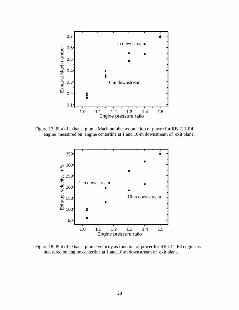
dropped as fuel flow increased. The plume mach number and hence, velocity, measured at 1 m

downstream of the exhaust plane increased dramatically with EPR (figs. 17 and 18), ranging

from 0.19 (velocity of 94 m s-1

) at idle to 0.7 (350 m s-1

) at 1.5 EPR. Polynomial fits to the

experimental data indicate that the 1-m downstream Mach number and velocity would be ~0.81

and 407 m s-1

) at 100 percent power (1.72 EPR).

Measurements recorded 10 m downstream of the engine exit suggest that although the plume

dilutes and cools fairly rapidly, it maintains a fairly high velocity for some distance behind the

plane (table 5). For example, carbon dioxide mixing ratios at 1.03 EPR are a factor of eight

fewer at 10-m than at 1-m (fig. 15), whereas the plume velocity only decreases 40% over this

distance (figs. 17 and 18). One may speculate that the disparity in the dilution of these

parameters is due to the mixing of bypass air with core flow from the combustor. The bypass

flow is expelled from the engine at roughly the same velocity as the core flow, but because it is

ducted around the compressor stages and combustor, it is relatively cool and does not contain

combustion byproducts.

4.2. Tracers and Hydrocarbons

Hydrocarbon measurements were made by UCI, Donald Blake, PI. In practice, 11 whole air

samples were collected in stainless steel canisters and shipped to UCI for analysis in their

analytical laboratory. Appendix B contains results and a discussion of the measurements

interpreted in terms of emission indices.

4.3. Gas-Phase HOHO and SOx Species

Aerodyne Research, Inc., in collaboration with NASA GRC deployed a TDL instrument

during EXCAVATE to determine exhaust plume nitrogen and sulfur species concentrations. The

TDL was located in the base of the sampling stand and its optical absorption cell was coupled to

the sampling manifold with a short piece of Teflon tubing, the goal being to maintain the sample

temperature at very high values to preserve any SO3 that may have formed in the combustor.

Appendix C reports the results of these measurements.

4.4. Particulate Physical Properties

Two groups working in collaboration determined the optical and microphysical properties of

engine aerosol emissions. NASA Langley deployed a condensation nuclei counter to measure

total aerosol concentrations, a dual differential mobility analyzer and an optical particle counter

11

to determine size distributions, and a particle soot absorption photometer to measure soot

concentrations. Appendix D reports the results of their study. UM used a nASA coupled with an

inlet heater to determine the size distribution of volatile and nonvolatile aerosols in the 3-100 nm

size range. Appendix E describes the results of their efforts.

4.5. Particle Composition

Aerodyne Research, Inc., operated an AMS during EXCAVATE. This instrument determines

the composition of individual aerosols in the 30-1000 nm size range as a function of

aerodynamic diameter. The instrument is particularly sensitive to organic, sulfate, and nitrate

species. Appendix F reports the results of the AMS study.

4.6. Ion Density and Chemi-ion Speciation

The AFGL contributed several instruments to the effort to characterize the aircraft engine

emissions: a chemical ionization mass spectrometer to assay gas-phase sulfur and nitrogen

species; a Gerdien tube condenser to determine total chemi-ion concentrations; and an electron

impact mass spectrometer to measure the chemi-ion mass spectrum. Appendix G reports the

results of their measurements.

5.0. References

Anderson, B., et al., 1999: Air Force F-16 Aircraft Engine Aerosol Emissions Under Cruise

Altitude Conditions, NASA/TM-1999-209192.

Baughcum, S. L., et al., 1996: Scheduled Civil Aircraft Emission Inventories for 1992: Database

Development and Analysis, NASA CR-4700.

Busen, R. and U. Schumann, 1995: Visible Contrail Formation from Fuels With Different Sulfur

Contents, Geophys. Res. Lett., 22, pp. 1357-1360.

Fahey, D., et al., 1995: Emission Measurements of the Concorde Supersonic Aircraft in the

Lower Stratosphere, Science, 270, pp. 70-74.

Friedl, R. (ed.), 1997: Atmospheric Effects of Subsonic Aaircraft: Interim Assessment Report of

the Advanced Subsonic Technology Program, NASA Ref. Publ. 1400.

Miake-Lye, R., et al., 1998: SOx Oxidation and Volatile Aerosol in Aircraft Exhaust Plumes

Depend on Fuel Sulfur Content, Geophys. Res. Lett., 25, pp. 1677-1680.

Schumann, U., et al., 1996: In Situ Observations of Particles in Jet Aircraft Exhausts and

Contrails for Different Sulfur Containing Fuels, J. Geophys. Res., 101, pp. 6853-6869.

Schumann, U., et al., 2002: Influence of Fuel Sulfur on the Composition of Aircraft Exhaust

Plumes: The Experiments SULFUR 1-7, J. Geophys. Res., Art. No. 4247, August.

Wey, C. C., et al., 1998: Engine Gaseous, Aerosol Precursor, and Particulate at Simulated Flight

Altitude Conditions, NASA TM-1998-208509, ARL-TR-1804.

Wyslouzil, B. E., et al., 1994: Observations of Hydration of Single Modified Carbon Aerosols,

Geophys. Res. Lett., 21, pp. 2107-2110.

Zheng, J., et al., 1994: An Analysis of Aircraft Exhaust Plumes From Accidental Eencounters,

Geophys. Res. Lett., 21, pp. 2579-2582.

12

Table 2 Sample Runs Behind Langley T-38A

Run Julian Percent Probe GMT GMT Sample Sample Gas probe Static T, Velocity,

number day power distance, m start end pressure CO2, ppm CO2, ppm C m/s

1 23 50 1 20:11:00 20:18:20

2 23 60 1 20:19:10 20:28:53

3 23 70 1 20:29:40 20:39:10

4 23 80 1 20:41:10 20:49:30

5 23 90 1 20:53:20 20:59:50

6 23 100 1 21:02:32 21:10:40

7 23 70 1 21:13:10 21:15:43

8 23 50 1 21:18:15 21:20:30

9 23 50 1 21:30:00 21:39:20

10 23 100 1 21:41:00 21:48:30

11 23 70 1 21:51:30 21:52:57

12 23 50 1 21:53:20 21:57:14

13 24 50 1 14:46:00 14:50:15 724 3395 3323 452.1

14 24 50 10 14:50:46 14:56:40 686 831 10383 452.8

15 24 60 10 14:58:00 15:03:00 688 1395 11962 389.3

16 24 60 1 15:06:20 15:12:50 726 2783 11189 375.7 87.2

17 24 70 1 15:13:20 15:18:15 733 3048 11206 326.3 138.6

18 24 70 10 15:18:40 15:28:30 687 1796 10741 324.8 141.2

19 24 80 10 15:30:30 15:35:10 703 2196 10847 306.9 216.0

20 24 80 1 15:36:30 15:43:45 788 2903 10809 306.6 214.3

21 24 90 1 15:46:20 15:48:50 865 4280 12456 306.7 334.8

22 24 90 10 15:50:55 15:59:00 727 1289 12468 304.9 334.8

23 24 100 10 15:59:40 16:05:30 728 1539 9706 345.6 450.1

24 24 100 1 16:07:10 16:14:35 890 4291 8904 336.5 443.7

25 24 70 1 16:16:12 16:19:30 763 2115 9531 310.6 136.0

26 24 70 10 16:20:40 16:29:30 726 1166 11018 313.3 131.2

27 24 50 10 16:30:40 16:34:00 716 2017 14144 453.9 19.1

28 24 50 1 16:35:50 16:39:20 732 3101 14262 450.9 10.5

29 29 50 1 14:43:20 14:48:15 718 4059 23583 56.7

30 29 50 1 14:49:30 14:52:40 750 2050 23740

31 29 50 1 14:55:00 14:59:20 762 651 23741

32 29 50 1 15:28:40 15:31:40 754 1704 23453 244.3 66.6

33 29 50 10 15:34:25 15:36:20 709 2630 24334 278.8 68.7

13

Table 2 Concluded

Run Julian Percent Probe GMT GMT Sample Sample Gas probe Static T, Velocity,

number day power distance, m start end pressure CO2, ppm CO2, ppm C m/s

34 29 50 1 15:39:10 15:39:40 707 3144 24254 268.5 71.1

35 29 60 1 15:42:20 15:45:00 721 3896 20841 233.5 83.5

36 29 60 1 15:45:20 15:48:35 757 1820 20903 232.9 83.8

37 29 60 1 15:48:50 15:52:10 768 634 20893 227.9 83.0

38 29 60 10 15:53:02 15:56:00 705 2388 20852 229.8 82.2

39 29 60 25 15:56:32 15:58:00 738 76 20813 225.9 82.0

40 29 60 1 15:58:30 15:59:20 755 1849 20795 225.9 82.4

41 29 70 1 16:00:50 16:03:15 742 3620 18653 197.2 118.7

42 29 70 1 16:03:50 16:06:35 771 2016 18687 193.8 118.0

43 29 70 1 16:07:04 16:10:16 784 978 18661 182.1 116.1

44 29 70 10 16:10:40 16:14:10 710 2652 18725 183.7 116.5

45 29 70 25 16:14:40 16:18:40 739 1376 18768 184.3 116.7

46 29 70 1 16:18:55 16:20:45 712 2672 18618 174.4 152.2

47 29 80 1 16:22:10 16:24:40 786 4048 18312 180.5 189.1

48 29 80 1 16:26:00 16:28:50 817 2110 18335 165.3 185.9

49 29 80 1 16:29:50 16:32:20 833 818 18321 168.8 186.6

50 29 80 10 16:32:35 16:36:15 725 1832 18359 168.6 186.1

51 29 80 25 16:36:30 16:39:25 739 1386 18359 169.3 189.6

52 29 90 1 16:40:45 16:43:06 818 3786 20735 244.1 313.8

53 29 90 1 16:44:00 16:46:40 842 2104 20540 245.0 315.4

54 29 90 1 16:47:10 16:50:20 902 953 20554 204.3 302.6

55 29 90 10 16:51:10 16:54:25 725 1951 20426 295.5 329.8

56 29 90 25 16:54:45 16:57:40 739 1378 20389 216.8 305.1

57 29 90 1 16:58:44 16:59:21 837 3404 20092 229.2 321.2

58 29 100 1 17:00:00 17:02:25 873 3973 27007 203.9 396.4

59 29 100 1 17:03:20 17:06:30 973 1980 28526 190.9 389.2

60 29 100 1 17:06:40 17:10:40 999 1348 28481 185.1 386.5

61 29 100 10 17:12:10 17:15:05 731 1977 28355 196.1 390.8

62 29 100 25 17:15:30 17:18:50 740 1502 27891 189.7 386.0

63 29 70 1 17:19:50 17:23:35 711 2725 18060 189.3 125.1

64 29 60 25 17:24:20 17:28:20 738 477 20886 200.4 82.2

65 29 60 10 17:28:34 17:29:20 714 2270 21752 210.5 78.5

66 29 50 10 17:29:20 17:35:00 714 1802 25011 246.9 59.9

14

Table 3 Sample Runs Behind Langley B-757

Run Julian Pressure Probe Fuel GMT GMT Sample Sample Gas probe Static T, Velocity,

number day ratio distance, m sulfur start end pressure CO2, ppm CO2, ppm C m/s

1 25 1.1 1 810 16:25:28 16:25:49 699 5785 191.9 155.5

2 25 1.15 1 810 16:26:10 16:27:13 736 5530 172.4 161.9

3 25 1.2 1 810 16:27:40 16:28:15 749 6018 79.7 167.7

4 25 1.25 1 810 16:28:30 16:29:25 753 7080 155.1 178.1

5 25 1.03 1 810 16:29:42 16:30:46 715 3584 229.1 81.0

6 25 1.03 1 810 16:44:40 16:45:36 749 2644 179.5 90.7

7 25 1.25 1 810 16:46:10 16:46:44 769 7765 207.4 219.4

8 25 1.3 1 810 16:48:00 16:49:10 803 5912 262.6 255.7

9 25 1.35 1 810 16:49:25 16:50:13 807 6845 283.0 280.8

10 25 1.4 1 810 16:50:30 16:50:50 822 7690 322.6 311.2

11 25 1.45 1 810 16:51:49 16:52:35 866 5306 365.7 342.7

12 25 1.5 1 810 16:52:50 16:53:38 869 5991 384.7 350.1

13 25 1.03 1 810 16:55:55 16:58:30 763 1091

14 25 1.03 10 810 19:00:00 19:01:04 718 740 2007

15 25 1.1 10 810 19:01:20 19:02:16 721 1060 2705

16 25 1.15 10 810 19:02:30 19:04:40 720 1261 3013 104.4

17 25 1.2 10 810 19:05:20 19:07:30 709 1937 3373 119.4

18 25 1.03 10 810 19:33:27 19:34:43 756 1636 7063 309.8 97.8

19 25 1.1 10 810 19:34:48 19:35:15 765 3764 16097 372.9 189.9

20 25 1.15 10 810 19:35:27 19:35:55 771 5214 16246 335.3 237.5

21 25 1.2 10 810 19:36:05 19:36:25 774 7087 16052 359.5 281.4

22 25 1.25 10 810 19:36:41 19:37:00 815 5668 16006 343.0 303.3

23 25 1.3 10 810 19:37:07 19:38:07 817 6244 23240 361.3 321.1

24 25 1.35 10 810 19:38:16 19:38:46 819 6902 24544 339.8 336.3

25 25 1.4 10 810 19:38:54 19:39:12 832 7633 25624 326.9 345.1

26 25 1.03 10 810 19:43:10 19:45:26 740 2502 17892 276.0 82.1

27 26 1.03 1 1050 14:37:49 14:40:39 736 3356 17395 300.7 99.9

28 26 1.03 1 1050 14:40:58 14:46:31 750 2704 17573 300.9 104.7

29 26 1.03 25 1050 14:47:03 14:52:46 746 775 17608 303.4 100.9

30 26 1.03 1 1050 14:53:15 14:54:51 748 2774 17592 313.6 114.0

31 26 1.15 1 1050 14:56:12 15:04:14 764 3767 21572 310.6 193.3

32 26 1.15 25 1050 15:04:25 15:10:20 745 811 21537 307.5 194.0

33 26 1.3 1 1050 15:11:10 15:18:30 823 3555 25827 314.9 266.4

15

Table 3 Continued

Run Julian Pressure Probe Fuel GMT GMT Sample Sample Gas probe Static T, Velocity,

number day ratio distance, m sulfur start end pressure CO2, ppm CO2, ppm C m/s

34 26 1.3 25 1050 15:18:41 15:24:15 682 1321 25714 311.9 265.6

35 26 1.3 1 1050 15:24:34 15:25:55 821 3606 25636 315.2 268.5

36 26 1.4 1 1050 15:26:30 15:34:28 831 3830 28274 313.7 304.8

37 26 1.4 25 1050 15:34:40 15:40:15 684 1522 28338 304.7 302.5

38 26 1.4 1 1050 15:40:34 15:41:30 837 3788 28304 308.2 308.3

39 26 1.5 1 1050 15:41:53 15:45:05 846 3734 30390 303.0 339.3

40 26 1.5 25 1050 15:45:15 15:46:50 706 1647 30954 301.1 333.6

41 26 1.03 25 1050 15:47:02 15:52:30 686 617 18773 329.4 97.3

42 26 1.03 1 1820 16:28:40 16:33:40 738 2894 18208 326.2 95.6

43 26 1.03 1 1820 16:34:05 16:39:50 677 4071 18370 314.0 94.1

44 26 1.03 25 1820 16:40:03 16:45:58 675 553 18433 322.0 94.1

45 26 1.03 1 1820 16:46:44 16:47:52 659 4160 18325 356.1 103.5

46 26 1.15 1 1820 16:48:55 16:56:01 786 2748 23239 321.1 188.9

47 26 1.15 25 1820 16:56:13 17:01:50 684 961 23602 326.2 190.2

48 26 1.15 1 1820 17:02:20 17:03:28 791 2692 23605 327.4 196.5

49 26 1.3 1 1820 17:04:03 17:11:50 821 3786 27500 325.3 269.2

50 26 1.3 25 1820 17:12:08 17:15:56 691 1236 27627 324.3 269.4

51 26 1.3 1 1820 17:16:11 17:18:50 822 3756 27661 328.1 271.4

52 26 1.4 1 1820 17:19:30 17:26:00 830 4143 30499 332.4 309.1

53 26 1.4 25 1820 17:26:05 17:33:00 691 1416 30521 337.7 310.2

54 26 1.4 1 1820 17:33:05 17:34:10 844 3031 30574 343.1 313.3

55 26 1.5 1 1820 17:34:15 17:37:10 840 3893 32282 346.6 350.0

56 26 1.5 25 1820 17:37:17 17:39:25 697 1564 32745 346.1 344.6

57 26 1.03 25 1820 17:40:00 17:43:15 698 469 18935 334.2 94.4

58 26 1.03 1 1820 17:43:56 17:44:51 728 2612 15578 277.4 81.0

59 26 1.03 1 1820 19:52:23 19:53:03 726 2592 16075 295.8 90.0

60 26 1.03 1 1820 19:53:23 20:03:50 661 4315 18549 320.6 91.5

61 26 1.03 25 1820 20:04:05 20:09:49 682 631 19004 329.3 91.2

62 26 1.03 1 1820 20:10:24 20:11:31 673 3898 19092 336.7 97.7

63 26 1.15 1 1820 20:12:48 20:19:55 785 2743 23709 330.7 190.8

64 26 1.15 25 1820 20:20:08 20:23:57 684 929 23544 330.0 190.3

65 26 1.15 1 1820 20:24:20 20:27:02 790 2609 23528 334.5 193.6

66 26 1.3 1 1820 20:27:32 20:36:06 822 3613 29183 352.2 275.0

16

Table 3 Continued

Run Julian Pressure Probe Fuel GMT GMT Sample Sample Gas probe Static T, Velocity,

number day ratio distance, m sulfur start end pressure CO2, ppm CO2, ppm C m/s

67 26 1.3 25 1820 20:36:16 20:41:00 692 1284 29081 352.8 275.0

68 26 1.3 1 1820 20:41:05 20:42:27 817 3740 29089 353.2 278.3

69 26 1.4 1 1820 20:42:52 20:49:57 837 3252 32244 369.3 317.2

70 26 1.4 25 1820 20:50:01 20:55:36 694 1482 32668 371.5 318.0

71 26 1.4 1 1820 20:56:20 20:57:51 838 3237 32604 373.7 321.0

72 26 1.5 1 1820 20:58:01 21:01:04 837 3913 35176 381.1 360.6

73 26 1.5 25 1820 21:01:14 21:03:14 693 1620 36179 378.4 346.2

74 26 1.03 25 1820 21:03:31 21:05:17 694 504 24720 388.3 95.9

75 26 1.03 1 1050 21:05:50 21:12:31 735 2876 17591 375.0 92.5

76 26 1.03 1 1050 21:13:13 21:15:15 737 2898 17260 351.7 90.5

77 26 1.03 1 1050 21:23:20 21:25:55 706 3121 17130 340.7 90.0

78 26 1.15 1 1050 21:27:05 21:32:15 783 2751 23571 340.4 191.0

79 26 1.15 25 1050 21:32:23 21:37:16 683 946 23407 340.0 191.1

80 26 1.15 1 1050 21:37:40 21:38:22 785 2792 23387 346.9 203.1

81 26 1.3 1 1050 21:38:33 21:43:58 822 3699 28113 361.8 276.8

82 26 1.3 25 1050 21:44:10 21:49:08 693 1264 29016 357.6 275.5

83 26 1.3 1 1050 21:49:23 21:50:50 824 3644 28941 357.6 277.3

84 26 1.4 1 1050 21:51:13 21:57:09 831 3958 32465 372.2 320.1

85 26 1.4 25 1050 21:57:19 22:01:51 691 1505 32710 370.9 319.4

86 26 1.4 1 1050 22:02:05 22:02:35 836 3910 32602 369.7 319.3

87 26 1.5 1 1050 22:03:39 22:06:04 838 3980 35122 374.8 356.7

88 26 1.5 25 1050 22:06:13 22:08:37 692 1673 35587 375.3 358.0

89 26 1.03 1 1050 22:13:20 22:17:55 636 4789 15963 316.7 88.3

90 26 1.03 25 1050 22:19:00 22:20:30 738 1315 16323 318.8 87.9

91 26 1.03 1 1050 22:25:26 22:26:04 610 5226 16096 278.6 78.3

92 27 1.03 1 810 13:44:15 13:46:25 710 4525 18115 289.5 93.3

93 27 1.03 1 810 13:47:07 13:47:44 579 6774 18989 313.7 100.1

94 27 1.03 1 810 13:48:54 13:54:10 665 4033 17488 290.5 94.6

95 27 1.03 1 810 13:55:20 14:01:28 755 1488 17665 292.4 95.7

96 27 1.03 1 810 14:02:17 14:05:45 767 428 17691 294.3 91.1

97 27 1.03 1 810 14:07:07 14:12:25 679 3923 17752 296.8 94.6

98 27 1.3 1 810 14:14:55 14:20:52 822 4027 25945 325.9 268.5

99 27 1.3 1 810 14:22:40 14:26:14 841 2005 26051 318.3 266.5

17

Table 3 continued

Run Julian Pressure Probe Fuel GMT GMT Sample Sample Gas probe Static T, Velocity,

number day ratio distance, m sulfur start end pressure CO2, ppm CO2, ppm C m/s

100 27 1.3 1 810 14:28:05 14:32:00 863 1017 26156 314.7 266.3

101 27 1.03 1 810 14:35:40 14:38:53 619 5101 17482 322.7 91.2

102 27 1.03 10 1050 15:22:03 14:41:20 630 1181 2153 47.8 62.7

103 27 1.03 35 1050 15:43:14 15:45:50 637 349 2107 47.5 55.5

104 27 1.03 10 1050 15:46:20 15:49:35 702 1331 3191 65.2 123.6

105 27 1.15 10 1050 15:48:33 15:53:04 682 1468 3216 63.2 128.1

106 27 1.15 35 1050 15:53:18 15:57:13 698 724 3249 64.7 128.6

107 27 1.15 10 1050 15:57:40 15:59:33 683 1456 3191 63.9 129.9

108 27 1.3 10 1050 16:01:30 16:05:04 794 1420 4841 83.5 180.9

109 27 1.3 35 1050 16:05:17 16:05:17 706 899 4871 84.4 181.0

110 27 1.3 10 1050 16:11:23 16:12:20 793 1498 4865 87.4 184.3

111 27 1.4 10 1050 16:13:05 16:15:05 822 1524 6358 98.9 211.5

112 27 1.4 35 1050 16:15:26 16:18:30 707 1124 6374 99.5 208.8

113 27 1.03 35 1050 16:19:16 16:20:56 701 319 2276 55.9 57.7

114 27 1.03 10 1050 16:21:45 16:23:54 613 1193 2101 50.4 56.2

115 27 1.03 10 1820 17:57:10 18:04:35 683 917 2228 54.5 57.7

116 27 1.03 35 1820 18:04:56 18:12:17 692 353 2110 66.2 61.5

117 27 1.03 10 1820 18:13:20 18:15:10 663 1048 2180 71.8 60.5

118 27 1.15 10 1820 18:16:20 18:20:50 757 904 3175 68.7 128.5

119 27 1.15 35 1820 18:22:56 18:25:18 745 450 3163 70.0 128.0

120 27 1.15 10 1820 18:25:40 18:28:33 760 880 3206 69.3 129.9

121 27 1.3 10 1820 18:28:55 18:34:30 782 1069 4910 89.5 179.5

122 27 1.3 35 1820 18:34:50 18:39:22 699 905 4917 90.5 182.1

123 27 1.3 10 1820 18:39:46 18:40:57 817 912 4997 91.2 181.1

124 27 1.4 10 1820 18:41:13 18:43:58 826 1107 6415 104.2 212.1

125 27 1.4 35 1820 18:44:20 18:47:20 697 1127 6620 105.3 213.6

126 27 1.03 10 1820 18:48:25 18:50:00 611 1227 2165 67.6 58.7

127 27 1.03 10 810 18:54:40 18:57:36 667 967 2108 52.9 57.5

128 27 1.03 35 810 18:57:50 19:04:34 694 394 2095 54.0 56.9

129 27 1.03 10 810 19:05:07 19:06:31 655 1065 2394 59.6 58.3

130 27 1.15 10 810 19:09:25 19:13:55 687 1366 3184 77.9 127.5

131 27 1.15 35 810 19:14:19 19:15:59 695 716 3233 110.4 134.0

132 27 1.15 10 810 19:16:17 19:18:58 746 1045 3193 69.8 127.9

18

Table 3 Concluded

Run Julian Pressure Probe Fuel GMT GMT Sample Sample Gas probe Static T, Velocity,

number day ratio distance, m sulfur start end pressure CO2, ppm CO2, ppm C m/s

133 27 1.3 10 810 19:19:24 19:25:26 757 1393 4887 92.6 185.4

134 27 1.3 35 810 19:27:00 19:30:48 697 920 4968 91.5 183.9

135 27 1.3 10 810 19:31:12 19:31:54 808 1243 5048 94.1 190.0

136 27 1.4 10 810 19:32:06 19:34:42 821 1316 6350 106.2 214.3

137 27 1.4 35 810 19:35:04 19:38:07 702 1099 6405 106.3 209.9

138 27 1.03 10 1820 19:39:05 19:50:36 626 1112 2113 77.8 62.8

139 27 1.03 35 1820 19:50:58 19:55:12 697 357 2212 71.9 61.3

140 27 1.03 10 1820 19:55:33 19:57:14 688 703 2097 72.5 63.8

141 27 1.15 10 1820 19:59:36 20:05:08 720 1220 3140 70.0 128.8

142 27 1.15 35 1820 20:05:30 20:08:52 698 707 3101 72.5 128.6

143 27 1.15 10 1820 20:09:20 20:09:48 729 1172 3044 85.5 144.3

144 27 1.3 10 1820 20:10:20 20:14:56 789 1630 4937 92.7 184.8

145 27 1.3 35 1820 20:15:39 20:20:12 697 959 4968 94.3 185.4

146 27 1.3 10 1820 20:20:42 20:22:05 782 1668 4962 95.2 188.6

147 27 1.4 10 1820 20:22:45 20:25:03 819 1552 6378 107.0 212.3

148 27 1.4 35 1820 20:25:26 20:28:24 709 1099 6442 107.2 208.3

149 27 1.03 10 1820 20:29:24 20:33:40 594 1244 2074 78.2 60.4

19

Table 4 List of J85-GE-5 Performance Characteristics Averaged Over All Runs

Engine power setting

50 60 70 80 90 100

Measured parameter AvgStd

devAvg

Std

devAvg

Std

devAvg

Std

devAvg

Std

devAvg

Std

dev

Fuel flow, kg/sec 0.066 - 0.077 - 0.090 - 0.122 - 0.172 - 0.268 -

Exhaust gas temp, deg C 500 - 430 - 405 - 430 - 500 - 640 -

Nozzle opening, percent 85 - 83 - 68 - 43 - 24 - 15 -

Exhaust CO2, percent 2.41 0.09 2.12 0.08 1.86 0.05 1.83 0.00 2.05 0.02 2.81 0.06

Exhaust Temp @ 1 m, deg C 403 53 363 36 300 35 302 48 341 34 409 36

Exhaust Mach number at 1 m 0.16 0.02 0.19 0.02 0.29 0.03 0.45 0.01 0.70 0.01 0.91 0.01

Exhaust velocity @ 1 m, m/s 70 15 86 10 132 13 197 13 321 12 413 28

Table 5 List of RB211-535E4 Performance Parameters Averaged Over All Data Runs

Engine pressure ratio

1.03 1.15 1.30 1.40 1.50

Measured parameter AvgStd

devAvg

Std

devAvg

Std

devAvg

Std

devAvg

Std

dev

Percent power 4.0 0.8 26.3 1.1 47.6 1.8 60.7 0.6 73.9 -

Low pressure fan speed, percent 23.5 0.2 53.3 1.2 72.1 0.6 80.4 0.7 86.1 -

Medium pressure fan speed, percent 34.2 0.4 63.8 0.4 76.3 1.5 80.6 0.5 84.0 -

High pressure fan speed, percent 53.8 0.7 75.4 0.9 82.8 0.8 85.6 0.5 88.0 -

Exhaust gas temp, deg C 355.6 29.2 456.2 11.7 547.5 15.0 599.6 8.7 638.0 -

Fuel flow, kg/s 0.14 0.01 0.46 0.02 0.81 0.03 1.04 0.01 1.29 -

Exhaust temperature @ 1 m, deg C 318.3 26.8 328.7 12.2 334.3 19.0 347.3 27.4 350.8 33.0

Exhaust CO2 @ 1 m, percent 1.76 0.10 2.32 0.08 2.74 0.14 3.10 0.18 3.36 0.22

Exhaust velocity @ 1 m, m/s 94.3 6.9 193.0 4.0 271.3 4.6 313.6 6.5 348.6 9.5

Exhaust Mach number @ 1 m 0.194 0.014 0.393 0.008 0.550 0.002 0.629 0.003 0.697 0.010

Exhaust temperature at 10 m, deg C 61.9 10.9 73.8 13.1 90.6 3.8 104.3 3.3 - -

Exhaust CO2 @ 10 m, percent 0.22 0.01 0.32 0.01 0.49 0.01 0.64 0.01 - -

Exhaust velocity @ 10 m, m/s 59.4 2.6 130.3 4.7 183.9 3.2 211.4 2.2 - -

Exhaust Mach number @ 10 m 0.162 0.008 0.349 0.014 0.481 0.010 0.543 0.007

20

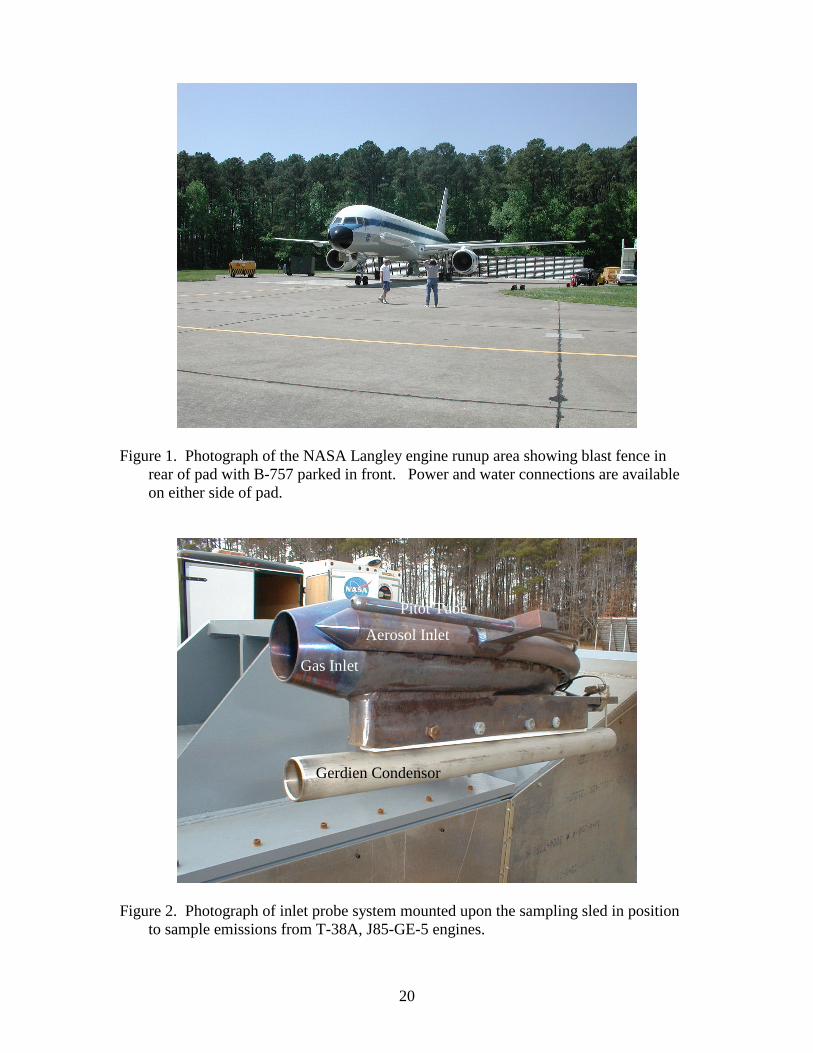
Figure 1. Photograph of the NASA Langley engine runup area showing blast fence in

rear of pad with B-757 parked in front. Power and water connections are available on either side of pad.

Pitot Tube

Aerosol Inlet

Gas Inlet

Gerdien Condensor

Figure 2. Photograph of inlet probe system mounted upon the sampling sled in position to sample emissions from T-38A, J85-GE-5 engines.

21

36”

18”R

GAS EXTRACTION PIPE

21/2” XXS Stain. Stl.

OD 2.875”

Wall .522”

ID Glass Coated

Particulate Extraction Probe

1.0” Tube

.095” Wall

30o

Dilution Gas

Typical Installation For Gas Extraction Probes

Unrestricted Vent to Atmosphere

Particulate Sample Transfer Tube: 5/8” OD .063” Wall

Langley EXCAVATE AEDC Proposed Concept 5/09/01

Pg 1 of 4

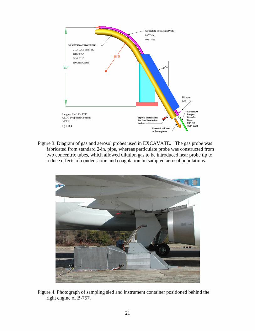
Figure 3. Diagram of gas and aerosol probes used in EXCAVATE. The gas probe was

fabricated from standard 2-in. pipe, whereas particulate probe was constructed from two concentric tubes, which allowed dilution gas to be introduced near probe tip to reduce effects of condensation and coagulation on sampled aerosol populations.

Figure 4. Photograph of sampling sled and instrument container positioned behind the

right engine of B-757.

22

Figure 5. Photograph of experimental setup showing B-757 with the sampling stand

positioned behind right engine and equipment trailers parked off right wing.

0 5000 10000 15000 20000 25000

50

60

70

80

90

100Jan 29Jan 24Jan 22

Per

cent

pow

er

1-second averaged data points

Figure 6. Plot of T-38A test sequence for 3 days on which its right engine was sampled.

23

0 5000 10000 15000 20000 25000 300000.9

1.0

1.1

1.2

1.3

1.4

1.5

1.6

Probe at 10 mProbe at 1 m

810 ppmS

1820 ppmS1050 ppmS

Eng

ine

pres

sure

rat

io

1-second averaged data points

Figure 7. Plot of B-757 test matrix showing power sequence and utilization of

different fuels.

50 60 70 80 90 100

0.05

0.10

0.15

0.20

0.25

0.30

Fue

l flo

w, k

g/s

Engine power, percent

Figure 8. Plot of fuel-flow rate versus power for J85-GE-5 engines on NASA T-38A aircraft.

24

50 60 70 80 90 100

1.8

2.0

2.2

2.4

2.6

2.8

3.0

Exh

aust

CO

2fr

actio

n, p

erce

nt

Engine power, percent

Figure 9. Plot of CO2 concentration versus power as measured on engine centerline, 1-m downstream of J85-GE-5 exit plane.

50 60 70 80 90 100

250

300

350

400

450

500

550

600

650

1 m downstream

Combustor exit

Exh

aust

gas

tem

pera

ture

, o C

Engine power, percent

Figure 10. Plot of exhaust gas temperatures for J85-GE-5 as measured at combustor exit

and 1 m downstream of exit plane.

25

50 60 70 80 90 100

0.2

0.4

0.6

0.8

1.0

Exh

aust

Mac

h nu

mbe

r

Engine power, percent

Figure 11. Exhaust gas Mach number versus power for J85-GE-5 engine as measured on

engine center line 1-m downstream of exit plane.

50 60 70 80 90 1000

50

100

150

200

250

300

350

400

450

Exh

aust

vel

ocity

, m

/s

Engine power, percent

Figure 12. Exhaust gas velocity versus power for J85-GE-5 engine as measured on

engine centerline 1-m downstream of exit plane.

26

1.0 1.1 1.2 1.3 1.4 1.50.0

0.2

0.4

0.6

0.8

1.0

1.2

1.4

Fue

l flo

w, k

g/s

Engine pressure ratio

Figure 13. Fuel-flow rate versus EPR for RB-211-E4 engines of B757.

1.0 1.1 1.2 1.3 1.4 1.5

0

10

20

30

40

50

60

70

80

Per

cent

pow

er

Engine pressure ratio

Figure 14. Plot of percent power versus EPR for RB-211-E4 engine, where relationship

between the two variables was established by fitting a third order polynomial to fuel flow/power data provided on most current ICAO engine qualification sheet (http://www.qinetiq.com/aircraft/aviation.html).

27

1.0 1.1 1.2 1.3 1.4 1.50.0

0.4

0.8

1.2

1.6

2.0

2.4

2.8

3.2

3.6

4.0

10 m downstream

1 m downstreamE

xhau

st C

O2,

per

cent

Engine pressure ratio

Figure 15. Carbon dioxide concentrations versus power as measured on engine center at

1 and 10-m downstream of RB-211-E4 exit plane.

1.0 1.1 1.2 1.3 1.4 1.50

100

200

300

400

500

600

700

10 m downstream

1 m downstream

Combustor exit

Exh

aust

tem

pera

ture

, o C

Engine pressure ratio

Figure 16. Plot of exhaust gas temperatures as function of power for RB-211-E4 engine

as measured at combustor exit and on engine centerline at 1 and 10-m downstream of the exit plane.

28

1.0 1.1 1.2 1.3 1.4 1.5

0.1

0.2

0.3

0.4

0.5

0.6

0.7

10 m downstream

1 m downstream

Exh

aust

Mac

h nu

mbe

r

Engine pressure ratio

Figure 17. Plot of exhaust plume Mach number as function of power for RB-211-E4

engine measured on engine centerline at 1 and 10-m downstream of exit plane.

1.0 1.1 1.2 1.3 1.4 1.5

50

100

150

200

250

300

350

10 m downstream

1 m downstream

Exh

aust

vel

ocity

, m

/s

Engine pressure ratio

Figure 18. Plot of exhaust plume velocity as function of power for RB-211-E4 engine as

measured on engine centerline at 1 and 10-m downstream of exit plane.

29

APPENDIX A: Performance Evaluation of Particle Sampling Probes

for Emission Measurements of Aircraft Jet Engines

Poshin Lee and David Y. H. Pui Particle Technology Laboratory,

Mechanical Engineering Department, University of Minnesota, Minneapolis, USA

Abstract

Considerable attention has been recently received on the impact of aircraft-produced aerosols upon global climate. Sampling particles directly from jet engines has been performed by different research groups in US and Europe. However, a large variation has been observed among published data on the conversion efficiency and emission indexes of jet engines. The variation results surely from the differences in test engine types, engine operation conditions, and environmental conditions. The other factor that could result in the observed variation is the performance of used sampling probes. Unfortunately, it is often neglected in the jet engine community. Particle losses during the sampling, transport and dilution processes are often not discussed/considered in literatures. To address this issue, we evaluated the performance of two sampling probes by challenging them with monodisperse particles. A significant performance difference was observed under different operation conditions. Thermophoretic effect, non-isokinetic sampling and turbulence loss contribute to the particle loss in the sampling probe. Keywords: aircraft exhaust, particle emission, sampling probe, jet engine Introduction It is known that atmospheric aerosols play a key role in the earth’s radiation balance, and thereby strongly influence global climate. Due to the heavy air travel nowadays, aircraft engines directly emit a great amount of both soot and sulfuric acid particles to the upper troposphere and lower stratosphere. These particles may have negative impact on climate through the processes of inducing the formation of new ice clouds (contrails), modifying physical properties of existing cirrus clouds, and providing additional surface area for heterogeneous chemical reactions such as ozone destruction.

In order to address this issue, researches have been performed to evaluate the emission of jet engines when aircrafts are either on ground or in air. To be able to understand the detail particle formation processes, sampling particles from jet engine exhaust or in the near field has been performed by NASA Subsonic aircraft Contrail and Cloud Effect Special Study (SUCCESS) and SULFUR series experiments by German agency, Deutsche Forschungsanstalt fur

Luft- and Raumfahut (DLR). For sulfate particle measurement, the values of ξ, the efficiency of conversion of fuel sulfate to sulfate in the forms of SO3 and H2SO4, by SUCCESS showed that ξ does not have a strong dependence with the fuel sulfur content (FSC) (1-3). In contrast, studies of DLR showed a decrease in ξ with an increase of FSC (4-5). These variations may result from the differences in engine types, engine operation conditions, environmental conditions, sampling and measuring methods (6). However, a significant difference is found by the comparison of non-volatile particle emission indices (EIs), the amount of pollutant generated per kilogram of fuel burned, measured in NASA B757 exhaust plumes (1, 2) during the SUCCESS project. Researchers began to suspect that the variation may result from the sampling probe design, sampling losses, and other uncertainties associated with particle size measurement. Unfortunately, the issue had not been addressed in all the related studies. The purpose of this study is focused on the experimental evaluation of the performance of sampling probe for the accurate measurement of jet engine particle emission.

30

Background

In this study, the performance of sampling probes is evaluated by the comparison of inlet and outlet concentrations. The dilution ratio is defined by the ratio of outlet flow rate, Qout, and inlet flow rates, Qin. And the particle penetration, P, is defined by

where Cin is the inlet concentration and Cout is the particle outlet concentration. Ideally, particle penetration should equal to 1 if there is no loss. Experimental Setup The setup of particle generation system is shown in Figure 1. The compressed air was first dry and cleaned by passing through a diffusion dryer and a HEPA filter before it is used in a collision type of atomizer. A flow rate of 2 lpm was controlled by the orifice installed in the atomizer. NaCl solutions were used in the atomizer. Two different solution concentrations, 1% and 0.1% (by weight), were used in order to provide the test particles in the sizes ranging from 20 to 200 nm. Polydisperse NaCl particle was produced by atomizing a NaCl solution and drying the airborne droplet stream by a diffusion dryer. For getting monodisperse particles, a nano-DMA with a high voltage power supply was used. By changing the DMA voltage and sheath flow rate, monodisperse particles of different particle sizes can be classified. In order to improve the control of excess and sheath flows of the classifer, a flow re-circulation loop between excess and sheath air ports was implemented as described in (7). The flow rate in the loop was set to be 5 and 15 lpm, so the maximum particle that can be classified is around 200 nm. Figure 2 shows the experimental setup for evaluating the sampling probe. Lindberg/Blue M (Asheville, NC) Module HTF55322A tube furnace with a ceramic tubing (5/8”(1.59cm) OD, 26”(66.04 cm) in length) was used to simulate the high temperature situation of real operation condition. Another Lindgerg/blue M tube furnace was used to heat up the dilution air. In high temperature testing, both furnaces were kept at 300 or 600 °C depending on the testing conditions. The head of test probes was

connected to ceramic tubing by Swage lock fitting and placed inside the furnace. The rest of the probe was insulated with a heating tape and insulation material. This arrangement allows the test probe temperature be maintained at 150 °C. It is also the air temperature inside the furnace. 2.5 feet of copper cooling coil and a ½” OD 10-feet copper tubing were connected after the probe to dissipating the heat before the concentration measurement by condensation particle counter. A clean dry air is used as dilution air and its maximum flow rate is 25 lpm. Two TSI 3025 condensation particle counters were used to measure the particle concentration upstream and downstream of the sampling probes. The actual dilution ratio at different particle sizes is then calculated from the upstream and downstream particle concentration readings.

Figure 1. Schematic of Particle Generation System

Figure 2. Experimental Setup

Blower

DiffusionDryer

Differential Pressure Gage 3

HEPA FilterRotameter 1

PressureRegulator

HEPA Filter

CompressedAir

Dryer

P

Rotameter 2

P

To Ambient (outlet 1)

Needle Valve 1

Needle Valve 2

Gauge 1

Gauge 2

Atomizer

Furnace

Condensationbottle

p

Sheath

Excess

HV

Monodisperse Aerosol (outlet 3)

Neutralizer

P

Nano DMA

Polydisperse Areosol (outlet 2)

Needle Valve 3

Differential Pressure Gage 1

p

CoolingCoil

Three wayvalve 1

Three wayvalve 2

Neutralizer

Probe Furnacesampling probe

Dilution air

Exit CPC (3025A)

Compressed Air

Mass flowmeterMass flowmeter

Compressed Air(or N2) house vacuum

Aerosol Calibration System

HEPA filter

HEPA filter

HEPA filter

3-way valve

dilution air furnace

rotameter

rotameter

Inlet CPC (3025A)

P

cooling coil (2.5 ft)10 ft 1/2" OD copper tubing

inin

outout

QC

QCP

××=

31

Results and Discussions Three different operation temperatures, 27, 300 and 600oC, were used in this study. The probe sampling flow rate was fixed at 5 lpm, and the dilution flow rate was changed to obtain a dilution ratio ranging from 1 to 7 depending on test conditions. Figure 3 shows the particle penetration through the sampling probe with different dilution ratios at room temperature. It is observed that the penetration at room temperature decreases as the increase of dilution ratios. Further, the loss is also increased as the particle size is reduced. This is normally the general trend of particle loss when turbulence mixing is occurred. Figure 4 and Figure 5 show the particle penetration with different dilution ratios at 300 and 600oC, respectively. In both cases, particle penetrations are lower than 70% for particle smaller than 50nm; however, it reaches a relatively stable value when the particle sizes are getting larger. Overall, the particle penetration can be higher than 70% for particles within 30 to 200 nm when different dilution ratios and operation temperatures are used. If we compare the same dilution ratio with different operation temperatures, the particle penetration decreases with the increase of operation temperature. The results are shown in Figure 6 and Figure 7 when dilution ratios are 1 and 7, respectively. It is because of more particle deposition on the inner wall of probe due to the particle thermophoretic effect. Conclusion and future works A significant performance differences were shown at different operation temperatures and dilution ratios. More works need to be done to further investigate the effect of thermophoresis on particle penetration through sampling probes. The particle loss increases with the increase of dilution ratios. From the observed trend of particle loss, it is evidenced that the turbulent mixing is happened inside the sampling probes. From the viewpoint of the mixing, the turbulent mixing is a need. On the other hand, the loss of particles, especially for nanometer particles, can be very significant under the turbulence flow condition. The balance between these two factors becomes a challenge for the future probe design. Our results show sampling probes do have a great influence on the accuracy of jet engine exhaust

Figure 3 Particle penetrations with Different Dilution Ratios at Room Temperature

Figure 4 Particle penetrations with Different Dilution Ratios at 300 0C

Figure 5 Particle penetrations with Different Dilution Ratios at 600 0C

0

0.2

0.4

0.6

0.8

1

0 50 100 150 200

Dilution Ratio: 1Dilution Ratio : 2Dilution Ratio: 3Dilution Ratio: 7

Par

ticl

e P

enet

ratio

n

Particle Size (nm)

0

0.2

0.4

0.6

0.8

1

0 50 100 150 200

Dilution Ratio: 1Dilution Ratio : 2Dilution Ratio: 3Dilution Ratio: 7

Pa

rtic

le P

ene

trat

ion

Particle Size (nm)

0

0.2

0.4

0.6

0.8

1

0 50 100 150 200

Dilution Ratio: 1Dilution Ratio : 2Dilution Ratio: 3Dilution Ratio: 7

Par

ticl

e P

enet

ratio

n

Particle S ize (nm )

32

Figure 6 Particle Penetrations at Different Operation Temperature (Dilution ratio: 1)

Figure 7 Particle Penetrations at Different Operation Temperature (Dilution ratio: 7) Reference 1. Anderson, B.E., W.R. Cofer, D.R. Bagwell, et

al., "Airborne Observations of Aircraft Aerosol Emissions I: Total Nonvalatile Particle Emission Indices," Geophysical Research Letters, 25(10): pp. 1689-1692(1998).

2. Hagen, D., P. Whitefield, J. Paladino, et al., "Particulate Sizing and Emission Indices for A Jet Engine Exhaust Sampled at Cruise,"

Geophysical Research Letters, 25(10): pp. 1681-1684(1998).

3. Miake-Lye, R.C., B.E. Anderson, W.R. Cofer, et al., "SOx Oxiidation and Volatile Aerosol in Aircraft Exhaust Plumes Depend On Fuel Sulfur Content," Geophysical Research Letters, 25(10): pp. 1677-1680(1998).

4. Schroder, F.P., B. Karcher, A. Petzold, et al., "Ultrafine Aerosol Particles in Aircraft Plumes: In Situ Observations," Geophysical Research Letters, 25(15): pp. 2789-2792(1998).

5. Karcher, B., F. Yu, F.P. Schroder, et al., "Ultrafine Aerosol Particles in Aircraft Plumes: Analysis of Growth Mechanisms," Geophysical Research Letters, 25(15): pp. 2793-2796(1998).

6. Kawa, S.R., J.G. Anderson, S.L. Baughcum, et al., "Assessment of the Effects of High-Speed Aircraft in the Stratosphere: 1998," NASA Technical Paper, 1999-209237(1999).

7. Chen, D.-R., D.Y.H. Pui, D. Hummes, et al., "Design and Evaluation of a Nanometer Aerosol Differential Mobility Analyzer (Nano-DMA)," J. Aerosol Sci., 29(5/6): pp. 497-509(1998).

0

0.2

0.4

0.6

0.8

1

0 50 100 150 200

Room temp300 C600 C

Par

ticl

e P

enet

rati

on

Particle Size (nm)

0

0.2

0.4

0.6

0.8

1

0 50 100 150 200

Room temp300 C600 C

Par

ticl

e P

en

etra

tio

n

Particle S ize (nm )

33

APPENDIX B: Hydrocarbon Emissions from a Modern Commercial Airliner

Bruce E. Anderson1, Donald R. Blake2, and Murray McEachern2

1-- NASA Langley Research Center

Hampton VA 23662

2-- University of California at Irvine Irvine California

1.0. Background Aircraft consume about 3 percent of the fossil fuels burned in the atmosphere each year, about 10 percent of this during landing and takeoff cycles (i.e., Friedl et al., 1997). Though the combustion of this fuel primarily produces carbon dioxide and water, a small fraction is emitted as non-methane hydrocarbons (NMHCs). These compounds are ozone precursors, can condense to form particles that impact visibility and inhibit respiratory function, and may be toxic or carcinogenic to exposed animal life. Though miniscule in comparison to the levels produced by automobiles and other surface-based transportation systems and judged to be relatively unimportant in ozone cycles at cruise altitudes (Friedl et al., 1997), aircraft NMHC emissions can potentially impact air quality and present a health hazard to workers, residents, and travelers within and around airport terminal areas. To understand, better predict, and mitigate the impact of aircraft operations upon local air quality, detailed information on NMHC emissions by aircraft is required. At present, such data are exceedingly sparse. The International Civil Aviation Organization (ICAO) does require that all commercial aircraft engines be emission qualified, meaning that their levels of CO, NOx, and total hydrocarbon (HC) emissions must be measured at idle, approach, climb out, and takeoff powers. However, HC measurements include contributions from methane and are not corrected for background ambient HC levels within intake air. In response this measurement need, several recent studies have determined NMHC speciation within turbine engine exhaust plumes. Spicer and coworkers investigated the emissions from both military,GE F101 and F110, (Spicer et al., 1992) and commercial engines, CFM-56-3, (Spicer et al., 1994) and found they generated cracking products, unburned fuel, and products of incomplete combustion at idle, with ethene, propene, acetylene and formaldehyde comprising 30~40 percent of the total emissions. At higher powers, relative NMHC emissions dropped by a factor of 20~50 and unburned fuel components disappeared. Slemr et al. (2001) report similar findings for an older technology engine, Rolls M 45H Mk501, and a more modern commercial high bypass turbo-fan, CFM 56-2C1, and note that the emission indices for these engines are highly power dependent and dominated by alkenes and alkynes related to fuel cracking and

34

aromatic compounds arising from unburned fuel. Both Slemr et al. (1998; 2001) and Spicer et al. (1992; 1994) note that NMHC emissions are likely dependent upon engine type, use, and maintenance history as well as fuel composition. Although the Spicer et al. (1994) and Slemr et al. (2001) studies provide significant insight into NMHC emissions from aircraft, their conclusions are drawn from limited sampling of just a few of the >300 types of commercial engines that are presently in use within the commercial aviation fleet and listed within the ICAO emissions database (www.qinetiq.com/aircraft/aviation.html). Clearly data from a broader range of engines are needed to provide a better statistical base for parameterizing aircraft NMHC emissions. For this reason, NMHC determinations were included as part of the measurement priorities for the NASA Experiment to Characterize Aircraft Volatile Aerosol and Trace Species Emissions (EXCAVATE). EXCAVATE was conducted during January 2002 with the primary objectives of characterizing the aerosol and aerosol precursor emissions from a modern commercial turbofan engine. The NASA Langley Boeing 757 that has a pair of Rolls Royce RB-211-535-E4 engines was used as the emission source. These engines produce over 40,000 lbs thrust, were designed for low-NOx and HC emissions and are used on ~80 percent of the B757 aircraft in service. Whole air samples were collected, both from the exhaust plume of one of these engines as it was operated at a variety of power settings, and from the background air being drawn into the engine intake. The samples were shipped to our laboratory at the University of California at Irvine where very sensitive gas chromatographic techniques were used to assay their halo- and hydrocarbon species content. We subsequently used these concentration data in concert with simultaneous engine CO2 emission measurements to calculate emission indices for each of the measured species. The paragraphs below describe our sample collection and analysis procedures and present the RB-211 NMHC emission observations. Results are compared to previous data sets and the implication of the measurements for aircraft operations poorly ventilated regions is explored.

2.0. Experiment

Whole air samples were collected in evacuated stainless steel canisters from the aerosol-sampling manifold that, in turn was connected to a stainless steel sample inlet positioned 10 m downstream and on the centerline of the B-757 engine exit plane. A total of 11 samples were collected, eight of engine emissions and three of background air in the vicinity of the aerosol instrument trailer. The set of canisters was subsequently shipped to UCI for detailed analysis of trace gas species.

Details of the analytical procedures employed by the UCI laboratory are given by Sive [1998], Colman et al. [2001], and Blake et al. [2003]. Aliquots of air from each canister were preconcentrated in a liquid nitrogen-cooled loop. This sample was directed to five different gas chromatographic column/detector combinations. Electron capture detectors (ECD, sensitive to halocarbons and alkyl nitrates), flame ionization detectors (FID, sensitive to hydrocarbons), and quadrupole mass spectrometers (MSD,

35

for unambiguous compound identification and selected ion monitoring) were employed. The first column–detector combination (abbreviated as “DB5ms/MSD”) was a DB5ms column (J&W; 60 m, 0.25 mm I.D., 0.5 µm film thickness) output to a MSD (HP-5973). The second combination (“DB1/FID”) was a DB-1 column (J&W; 60 m, 0.32 mm I.D., 1 µm film thickness) output to a FID (HP-6890). The third combination (“PLOT-DB1/FID”) was a PLOT column (J&W GS-Alumina; 30 m, 0.53 mm I.D.) connected in series to a DB-1 column (J&W; 5 m, 0.53 mm I.D., 1.5 µm film thickness) and output to an FID. The fourth combination (“Restek1701/ECD”) was a RESTEK 1701 column (60 m, 0.25 mm I.D., 0.50 µm film thickness), which was output to an ECD. The fifth combination (“DB5-Restek1701/ECD”) was a DB5 (J&W; 30 m, 0.25 mm I.D., 1 µm film thickness) column connected in series to a RESTEK 1701 column (5 m, 0.25 mm I.D., 0.5 µm film thickness) and output to an ECD. The DB5ms/MS, DB1/FID, PLOT-DB1/FID, Restek1701/ECD, and DB5-Restek1701/ECD combinations received 10.1 percent, 15.1 percent, 60.8 percent, 7.2 percent, and 6.8 percent of the sample flow, respectively. Our analytical accuracy ranges from 2 percent to 20 percent. The precision of the measurements varies by compound and by mixing ratio. For example, the measurement precision is 1 percent or 1.5 pptv (whichever is larger) for the alkanes and alkynes, and 3 percent or 3 pptv (whichever is larger) for the alkenes (Sive, 1998). The precision for the alkyl nitrates was better than 2 percent at the levels observed during the Pacific Exploratory Mission-Tropical Phase (Colman et al., 2001). The precision for C2Cl4 at 5 pptv is ±0.05 pptv (Colman et al., 2001). The limit of detection (LOD) is 3 pptv for the NMHCs. The alkyl nitrate detection limit was 0.02 pptv (except 0.01 pptv for methyl nitrate) (Colman et al., 2001). C2Cl4 was present at mixing ratios well above its detection limit at all times. The canister air was also analyzed for CO using GC with FID, as described by Hurst [1990] and Lopez [2002] using a packed column GC separation of CO followed by reduction to methane on a nickel catalyst and detection by FID. The absolute accuracy of the CO measurements calibrated against NIST standards was ±7 percent, with a DL of 5 ppbv (Lopez, 2002).

3.0. Results

Along with run specific information, Table 1 lists the dilution-corrected mixing ratios of 56 carbon species that were measured in each of the 11 samples collected during EXCAVATE. Note that eight of the samples were obtained from the engine exhaust plume as it ran at four different power settings (1.03, 1.15, 1.3 and 1.4 engine pressure ratios, where 1.03 is idle and 1.4 is cruise) and burned two fuels that were different in both hydrocarbon and sulfur content. Three samples are of background air, collected to determine the ambient concentrations of each of the measured species. The CO2 values shown in the list were determined using two different nondispersive infrared instruments, one monitoring concentrations in the dry N2-diluted sample air that was aspired into the whole-air canisters and the other measuring mixing ratios in undiluted air collected from the engine exhaust with a separate inlet probe. The ratio of the CO2 concentrations yield the sample dilution ratios that were used for correcting the carbon species concentrations to those that would have been observed in undiluted exhaust flow 10 meters behind the engine exhaust plane. We estimate that the dilution factors derived in this manner are accurate to +20 percent.

36

Table 2 provides averages of the carbon species mixing ratios, comparing values obtained in the exhaust plume at idle (1.03 EPR) and higher powers (1.15 + 1.30 + 1.40) with the average of measurements from the first two samples collected in from background air. We chose to disregard the third background sample because it contained high levels of several reactive species (i.e., HCFC 22, n-Heptane, n-hexane, benzene, toluene), suggesting that the air mass from which it was extracted was recently exposed to some unknown pollution source.

Table 3 lists mass emission indices (EIs) in units of g kg-1 fuel burned for CO and CH4 and µg kg-1 fuel burned for the remainder of the measured species. EIs were calculated using the following formula:

EIx = EICO2 x ∆(X)/∆(CO2) x (AMUx)/(AMUCO2) Eq. 1

where EICO2 is calculated from the fuel carbon content assuming combustion to be 100 percent efficient, ∆(X) and ∆(CO2) are the enhancements of compound X and CO2 within the plume, respectively, and AMUx and AMUCO2 are the molecular weights of X and CO2, respectively. A nominal value of 3160 g kg-1 fuel burned was used for EICO2 in all the calculations. ∆(X) values were determined by subtracting average background mixing ratios of X from the dilution corrected values measured in the plume. Cases where X was consumed within the combustor yielded negative EI values.

Examining the tables we note that CO and CH4 are by far the most abundant trace carbon species in engine exhaust, the former arising from incomplete combustion of jet fuel and the latter derived primarily from background air. At engine idle, CO comprises almost 2 percent of the exhaust emissions, but contributes <0.1 percent at high EPRs indicating that the engine runs much more efficiently at the higher temperatures and pressures associated with high power settings. Its emission indices, EIco, was 12 and ~16 g kg-1 for the two samples taken at idle and between 0.6 and 0.8 g kg-1 in samples acquired at power settings more typical of cruise and climb out (1.3 – 1.4 EPR). These compare extremely well to the RB211-535E4 values archived in the International Civil Aviation Organization (ICAO) Engine Emissions Data Bank (http://www.qinetiq.com/aircraft/aviation.html) of 13 – 16 g kg-1 for idle; 1.1 – 2.7 g kg-1 for approach; 0.5 – 1.2 g kg-1 for climb out; and 0.7 to 1.0 g kg-1 for take off. Simultaneous aerosol measurements suggest that the engine’s efficiency varies significantly just after engine start and when power is reduced from higher settings to idle so that any single grab sample taken at idle would not necessarily be representative of the average emissions at that power setting. The ICAO values are averaged over several minutes of engine operation, which may explain why one of our instantaneous idle readings was 50 percent above their range of published values.

Regarding CH4, its concentrations were typically not more than 20 percent higher than ambient values at engine idle and tended to drop off with increasing engine powers, with some mixing ratios being lower than ambient values (Table 1) which suggests that under some conditions the engine actually burns methane out of the background air.

37

This observation is not surprising, since negative methane emission indices were observed for this same aircraft in flight during the SUCCESS mission (Vay et al., 1998) and Spicer et. al., (1992) note that most high efficiency engines tend to produce minor amounts of CH4 at idle and consume it at higher engine powers. Correcting for background mixing ratios, EICH4 varied from –0.09 to 0.3 g kg-1. The ICAO database does not report EIs for this species, but we suspect that the positive values calculated for higher engine powers may be caused by either errors in the dilution ratio or variations in the background mixing ratio of CH4. Note that the sample that yielded the greatest EICH4 also exhibited significantly positive EIs for a number of halocarbon species suggesting the background air at the time was more polluted than average. Also, for the plume dilutions that we were dealing with, a 20 percent error in the calculated dilution ratio equates to a variation of 0.1 to 0.2 g kg-1 in EICH4. In any case, our results and those of others (Spicer et al., 1992; Spicer et al., 1994; Vay et al., 1998; and Slemr et al., 2001) suggest that turbine engines are not a significant source of CH4.

In terms of other species, the fuels burned during EXCAVATE contained varying levels of sulfur contaminants, for the two cases sampled here, 810 and 1820 ppm by weight. Thus, sulfur compounds should be prevalent within the engine exhaust. Indeed, mixing ratios for OCS and CS2 were two to five times higher in the exhaust plume than within ambient air and appeared to show a slight trend with fuel S content. However, their EIs were several orders of magnitude lower than SO2, the primary sulfur species emitted by the aircraft (Wormhoudt et al., Appendix C of this report). DMS, like CH4, was depleted in most samples collected at high engine powers suggesting that the engine consumes this species from background air at high combustor temperatures.

As for halocarbon emissions, of the 16 species assayed, 14 were either unchanged or depleted within the engine exhaust relative to ambient air (Tables 1 and 2). Only CH3Cl and CH3Br exhibited slight enhancements, but these were less than a factor of two above average background mixing ratios and may have been related to ambient variability rather than formation from fuel components. However, biomass burning is known to generate these species (Blake et al., 2003) so it is conceivable that they are produced within the combustor, either from fuel components or the oxidation of species from within the background air.

Hydrocarbon-nitrate species were slightly enhanced within the plume. Of the five species measured, methyl nitrate was most abundant, both within the plume and background air. Its average mixing ratio was three fold higher than ambient at high power (1.4 EPR), five times higher at idle (1.03), but tended to be somewhat depleted at medium powers (1.15 and 1.3). Nonmethane hydrocarbon concentrations decrease with engine power whereas NOx increases; the product of the two is at a minimum at the settings where we see lower RNO2 values. As for EIs, the sum for all five species is < 0.0005 g kg-1 at idle and < 0.0001 g kg-1 at 1.4 EPR. Comparing this to the RB211-535-E4 ICAO values of 4 g kg-1 and ~18 g kg-1 NOx at idle and climbout power, respectively, we conclude that an insignificant amount of aircraft emissions are sequestered as RNOx species.

38

The remaining species listed in the tables are hydrocarbons and showed a great range of enhancement ratios within the engine exhaust plume relative to background air. Data are presented for 27 NMHC species with two to nine carbon atoms. Figure 1 shows that at idle, the engine primarily emits species containing two to four carbon atoms, but when engine power is increased to 1.4 EPR, light hydrocarbon emissions are greatly reduced and the peak in the carbon emission distribution shifts out to seven atoms (heptane +toluene). Spicer et al. (1994) notes that jet fuel is primarily composed of species with five or more carbons and, by weight, 70 percent of the compounds it contains has 11 to 14 carbons. Thus, the low molecular weight species found in the exhaust are derived from reactions occurring within the combustor rather than being residual, unburned fuel. Aromatics are present in the fuel but are also byproducts of incomplete hydrocarbon oxidation, thus the enhancements in benzene and toluene mixing ratios can be either “combustion” or “fuel” derived.

Table 4 provides a summary of the NMHC emissions from the RB211 engine for each of the exhaust samples, broken down into the functional groupings of alkanes (all single bonded hydrocarbons), alkenes (at least one double bond), alkynes (at least one triple bond), and aromatics (benzene ring compounds). Figure 2 shows a plot of the fraction of the NMHCs emitted in each functional group over the range of engine power settings. At idle (1.03 EPR) > 90 percent of the emissions are double or triple-bonded, straight chain hydrocarbons, whereas at high power, these compounds account for < 20 percent of the total. The fractional contribution of aromatics grows from < 10 percent to > 50 percent as power is increased from idle to climb-out settings, respectively. Alkanes are the least abundant species at low power but generally comprise 20 to 40 percent of the total NMHC mass emissions at high powers.

In terms of individual species, at idle, the most abundant were ethene, ethyne, and propene. Their mixing ratios were enhanced by factors of 200 to 1000 above those measured in ambient air, and, taken together, accounted for 88 percent of the measured NMHC emissions on a molar basis. Ethene alone accounted for 57 percent of the emissions that were quantified. Excluding contributions from oxygenated HC species that we did not measure, this is consistent with observations from military engines acquired by Spicer et al. (1992) and the CFM-56-2 engines of the NASA DC-8 by Slemr et al. (2001). At higher engine powers, the light hydrocarbon species all but disappear, and n-heptane and toluene become more dominant. As noted above, these could be either fuel or combustion derived.

As shown in Table 4 and illustrated in Figure 3, total NMHC emissions drop off precipitously as power is increased. At idle, the engine emits ~1 g kg-1 of 2 – 9 carbon HC compounds, whereas at 1.4 EPR, which is essentially climb-out power, it produces ~0.005 g kg-1, or about factor of 200 less. Similar reductions were apparent in the CO emissions (Table 3 and Figure 3). Variations in CO and NMHC EIs were highly correlated (Figure 4) which one might expect for incomplete combustion at low engine temperatures.

39

Comparing our total NMHC EIs with ICAO data, we find relatively good agreement at idle, but that EXCAVATE values tend to be somewhat lower at higher engine powers. The ICAO archive reports values of 0.4-1, 0.04, and 0.01 g kg-1 at idle, approach, and climb-out, respectively. These compare to our observations of 0.5—1, ~0.01, and ~0.005 g kg-1 for roughly the same power settings, respectively. ICAO engine emission qualification tests are performed with multi-gas analyzers that give an integrated signal proportional to the total hydrocarbons present in the sample. Thus, differences between the EXCAVATE and ICAO values can probably be attributed to contributions from species, such as oxygenated HC compounds, that we did not measure as well as the fact that ICAO data are not corrected for ambient NMHC contributions. We note that Spicer et al. (1994) resolved 182 chromatographic peaks in samples collected in the exhaust of a CFM-56 engine and found significant amounts of formaldehyde, acetaldehyde, and acetone that, at high power settings, accounted for > 50 percent of the total NMHC emissions.

Two separate batches of JP-5 fuel were burned in the tests, thus one might expect to see some systematic differences in the NMHC emissions based on the differences in the fuel hydrocarbon matrices. Examining Table 4, we see that total NMHC emissions were slightly higher for 1820 ppm S fuel than the 810 ppm S fuel. These differences are particularly notable at idle where the total NMHC EI for the high S fuel is ~two times (1.1 g kg-1 vs. 0.55 g kg-1) that of the low sulfur fuel. Though these differences are significant, they may not reflect fuel-induced effects. Simultaneous aerosol measurements show that the engine emissions are highly variable at low powers, with mass emissions decreasing by more than an order of magnitude in the 10 minutes after engine start. The low S samples were collected after more than an hour of continuous runtime and may simply reflect the fact that the engine runs more efficiently after it has warmed up. Clearly more measurements are needed to discriminate fuel matrix from operational parameter impacts on NMHC emissions.

4.0. References

Blake, N. J., D. R. Blake, A. L. Swanson, E. Atlas, F. Flocke, and F. S. Rowland, 2003: Latitudinal, vertical, and seasonal variations of C1–C4 alkyl nitrates in the troposphere over the Pacific Ocean during PEM-Tropics A and B: Oceanic and continental sources. J. Geophys. Res., doi:10.1029/2001JD001444.

Civil Aviation Authority, 2002-2004: ICAO aircraft engine emissions databank, Civil Aviation Authority Web Site. http://www.qinetiq.com/aircraft/aviation.html.

Colman, J. J., A. L. Swanson, S. Meinardi, B. C. Sive, D. R. Blake, and F. S. Rowland, 2001: Description of the analysis of a wide range of volatile organic compounds in whole air samples collected during PEM-Tropics A and B. Anal. Chem., 73, pp. 3723–3731.

Hurst, D. F., 1990: Seasonal variations in the latitudinal distribution of tropospheric carbon monoxide, 1986–1988. Dissertation, Univ. of Calif., Irvine.

40

Lopez, J. d. P., 2002: Seasonality and global growth trends of carbon monoxide during 1995–2001. Ph.D. thesis, Univ. of Calif., Irvine, Irvine.

Sive, B. C., 1998: Analytical methods and estimated hydroxyl radical concentrations. Ph.D. thesis, Univ. of Calif., Irvine, Irvine.

Slemr, F., et al., 1999: In-flight measurement of aircraft non-methane hydrocarbon emission indices. Geophys. Res. Lett., 26, pp.3053-3056.

Slemr, F., et al., 1998: In-flight measurement of aircraft non-methane hydrocarbon emission indices. Geophys. Res. Lett., 25(3), pp. 321-324.

Slemr, F., et al., 2001: In-flight measurements of aircraft CO and nonmethane hydrocarbon emission indices. J. Geophys. Res., 106, pp. 7485-7494.

Spicer, C.W., et. al., 1992: Chemical composition of exhaust from aircraft turbine engines. J. Eng. Gas Turbines Power, 114, pp. 111-115.

Spicer, C.W, et. al., 1994: Chemical composition and photochemical reactivity of exhaust from aircraft turbine engines. Ann. Geophys., 12, pp. 944-955.

Vay, S.A., et al., 1998: DC-8-based observations of aircraft CO, CH4, N2O, and H2O (g) emission indices during SUCCESS. Geophys. Res. Lett., 25, pp. 1717-1720.

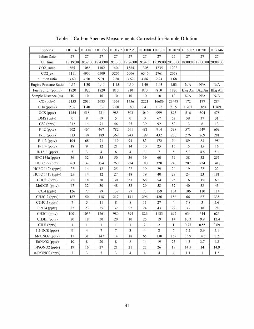
41

Table 1. Carbon Species Measurements Corrected for Sample Dilution

Species DE1149 DE1181 DE1166 DE1062 DE2358 DE1008 DE1302 DE1020 DE6602 DE7010 DE7146

Julian Date 27 27 27 27 27 27 27 27 27 27 27

UT time 18:19:30 18:32:00 18:43:00 19:13:00 19:26:00 19:34:00 19:39:00 20:30:00 18:00:00 19:00:00 20:00:00

CO2_samp 865 1088 1102 1404 1384 1305 1235 1222

CO2_ex 3111 4900 6509 3206 5006 6346 2761 2058

dilution ratio 3.60 4.50 5.91 2.28 3.62 4.86 2.24 1.68

Engine Pressure Ratio 1.15 1.30 1.40 1.15 1.30 1.40 1.03 1.03 N/A N/A N/A

Fuel Sulfur (ppmv) 1820 1820 1820 810 810 810 810 1820 Bkg Air Bkg Air Bkg Air

Sample Distance (m) 10 10 10 10 10 10 10 10 N/A N/A N/A

CO (ppbv) 2153 2030 2683 1363 1756 2221 16686 23448 172 177 284

CH4 (ppmv) 2.32 1.40 1.39 2.60 1.80 2.41 1.95 2.15 1.707 1.854 1.769

OCS (pptv) 1454 518 721 985 503 1040 999 895 516 504 478

DMS (pptv) 0 9 59 5 0 0 67 52 59 37 31

CS2 (pptv) 212 14 71 46 25 39 92 52 13 6 13

F-12 (pptv) 702 464 467 782 561 481 914 598 571 549 609

F-11 (pptv) 313 194 189 369 243 199 432 286 276 269 281

F-113 (pptv) 104 68 71 119 94 83 172 94 89 83 98

F-114 (pptv) 18 9 12 21 14 10 25 15 15 15 16

H-1211 (pptv) 5 3 4 6 4 3 7 5 5.2 4.8 5.1

HFC 134a (pptv) 36 32 35 50 36 39 60 39 38 32 255

HCFC 22 (pptv) 263 149 154 260 224 180 320 240 207 224 1417

HCFC 142b (pptv) 22 14 12 25 22 19 29 20 19 22 22

HCFC 141b (pptv) 25 14 12 27 18 19 40 29 24 23 181

CHCl3 (pptv) 25 18 30 30 33 68 54 25 16 15 69

MeCCl3 (pptv) 47 32 30 48 33 29 58 37 40 38 43

CCl4 (pptv) 126 77 89 137 87 73 159 104 106 110 114

CH2Cl2 (pptv) 187 50 118 217 141 296 426 156 66 67 338

C2HCl3 (pptv) 7 5 11 8 8 11 27 4 7.8 3 5.6

C2Cl4 (pptv) 32 23 35 32 22 24 43 22 33 18 28

CH3Cl (pptv) 1001 1035 1761 980 594 826 1133 692 634 644 626

CH3Br (pptv) 20 18 30 20 10 25 19 14 10.3 9.9 12.4

CH3I (pptv) 1 1 1 1 1 2 2 1 0.75 0.55 0.69

1,2-DCE (pptv) 9 4 7 7 3 4 8 6 5.2 3.9 5.1

MeONO2 (pptv) 17 31 147 14 18 65 130 169 33.9 14.8 8.2

EtONO2 (pptv) 10 8 20 8 8 14 19 23 4.5 3.7 4.8

i-PrONO2 (pptv) 19 16 27 21 21 22 26 19 14.5 14 14.9

n-PrONO2 (pptv) 3 3 5 3 4 4 4 4 1.1 1 1.2

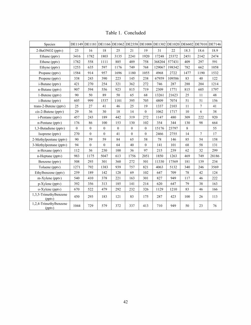
42

Table 1. Concluded

Species DE1149 DE1181 DE1166 DE1062 DE2358 DE1008 DE1302 DE1020 DE6602 DE7010 DE7146

2-BuONO2 (pptv) 23 16 18 25 21 19 31 22 18.3 18.6 18.9

Ethane (pptv) 3416 1782 1803 3135 2241 1920 17248 23372 2451 2142 2474

Ethene (pptv) 1782 558 1111 885 489 758 368204 577431 409 297 591

Ethyne (pptv) 1253 635 597 1176 749 768 129067 198342 782 662 1058

Propane (pptv) 1584 914 957 1696 1180 1055 4968 2722 1477 1190 1532

Propene (pptv) 338 243 390 223 145 238 67959 109586 83 40 122

i-Butane (pptv) 421 270 254 321 362 272 746 287 288 204 1214

n-Butane (pptv) 907 594 556 923 815 719 2309 1771 815 605 1797

1-Butene (pptv) 90 50 89 50 65 68 13261 21623 25 11 48

i-Butene (pptv) 605 999 1537 1101 395 705 4809 7074 51 51 156

trans-2-Butene (pptv) 25 27 41 46 25 19 1337 2103 11 7 41

cis-2-Butene (pptv) 29 36 30 18 14 0 1062 1717 10 6 38

i-Pentane (pptv) 457 243 189 442 319 272 1147 480 309 222 920

n-Pentane (pptv) 176 86 100 153 130 102 354 344 130 98 664

1,3-Butadiene (pptv) 0 0 0 0 0 0 15176 23797 8 55

Isoprene (pptv) 270 0 0 41 0 0 2466 2755 14 7 17

2-Methylpentane (pptv) 90 59 59 84 65 58 78 146 85 54 158

3-Methylpentane (pptv) 94 0 0 64 40 0 141 101 68 58 131

n-Hexane (pptv) 112 36 230 100 36 97 215 239 62 32 299

n-Heptane (pptv) 983 1175 5047 613 1756 2051 1850 1263 469 749 28186

Benzene (pptv) 508 293 301 360 272 501 11330 17569 181 139 234

Toluene (pptv) 1271 792 1383 939 757 821 4063 5132 340 246 3569

Ethylbenzene (pptv) 259 189 142 128 69 102 647 709 78 42 124

m-Xylene (pptv) 540 410 378 221 163 301 827 949 117 46 222

p-Xylene (pptv) 392 356 313 185 141 214 620 647 79 38 163

o-Xylene (pptv) 670 522 479 292 232 326 1129 1210 83 46 166

1,3,5-Trimethylbenzene

(pptv)450 293 183 121 83 175 287 423 100 26 113

1,2,4-Trimethylbenzene

(pptv)1044 729 579 372 337 413 710 949 50 23 76

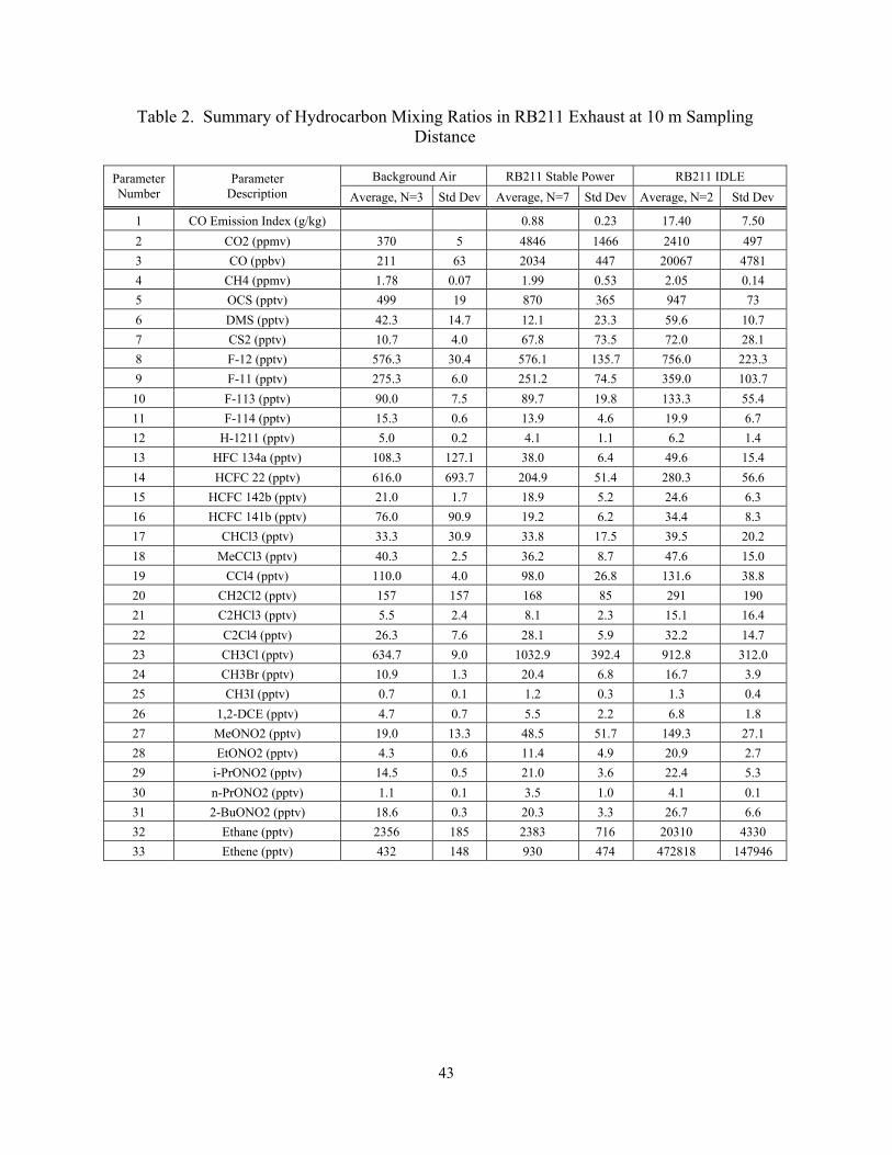
43

Table 2. Summary of Hydrocarbon Mixing Ratios in RB211 Exhaust at 10 m Sampling

Distance

Background Air RB211 Stable Power RB211 IDLEParameter

Number

Parameter

Description Average, N=3 Std Dev Average, N=7 Std Dev Average, N=2 Std Dev

1 CO Emission Index (g/kg) 0.88 0.23 17.40 7.50

2 CO2 (ppmv) 370 5 4846 1466 2410 497

3 CO (ppbv) 211 63 2034 447 20067 4781

4 CH4 (ppmv) 1.78 0.07 1.99 0.53 2.05 0.14

5 OCS (pptv) 499 19 870 365 947 73

6 DMS (pptv) 42.3 14.7 12.1 23.3 59.6 10.7

7 CS2 (pptv) 10.7 4.0 67.8 73.5 72.0 28.1

8 F-12 (pptv) 576.3 30.4 576.1 135.7 756.0 223.3

9 F-11 (pptv) 275.3 6.0 251.2 74.5 359.0 103.7

10 F-113 (pptv) 90.0 7.5 89.7 19.8 133.3 55.4

11 F-114 (pptv) 15.3 0.6 13.9 4.6 19.9 6.7

12 H-1211 (pptv) 5.0 0.2 4.1 1.1 6.2 1.4

13 HFC 134a (pptv) 108.3 127.1 38.0 6.4 49.6 15.4

14 HCFC 22 (pptv) 616.0 693.7 204.9 51.4 280.3 56.6

15 HCFC 142b (pptv) 21.0 1.7 18.9 5.2 24.6 6.3

16 HCFC 141b (pptv) 76.0 90.9 19.2 6.2 34.4 8.3

17 CHCl3 (pptv) 33.3 30.9 33.8 17.5 39.5 20.2

18 MeCCl3 (pptv) 40.3 2.5 36.2 8.7 47.6 15.0

19 CCl4 (pptv) 110.0 4.0 98.0 26.8 131.6 38.8

20 CH2Cl2 (pptv) 157 157 168 85 291 190

21 C2HCl3 (pptv) 5.5 2.4 8.1 2.3 15.1 16.4

22 C2Cl4 (pptv) 26.3 7.6 28.1 5.9 32.2 14.7

23 CH3Cl (pptv) 634.7 9.0 1032.9 392.4 912.8 312.0

24 CH3Br (pptv) 10.9 1.3 20.4 6.8 16.7 3.9

25 CH3I (pptv) 0.7 0.1 1.2 0.3 1.3 0.4

26 1,2-DCE (pptv) 4.7 0.7 5.5 2.2 6.8 1.8

27 MeONO2 (pptv) 19.0 13.3 48.5 51.7 149.3 27.1

28 EtONO2 (pptv) 4.3 0.6 11.4 4.9 20.9 2.7

29 i-PrONO2 (pptv) 14.5 0.5 21.0 3.6 22.4 5.3

30 n-PrONO2 (pptv) 1.1 0.1 3.5 1.0 4.1 0.1

31 2-BuONO2 (pptv) 18.6 0.3 20.3 3.3 26.7 6.6

32 Ethane (pptv) 2356 185 2383 716 20310 4330

33 Ethene (pptv) 432 148 930 474 472818 147946

44

Table 2. Concluded

Background Air RB211 Stable Power RB211 IDLEParameter

Number

Parameter

Description Average, N=3 Std Dev Average, N=3 Std Dev Average, N=2 Std Dev

34 Ethyne (pptv) 834 203 863 281 163705 48985

35 Propane (pptv) 1400 184 1231 332 3845 1589

36 Propene (pptv) 81.7 41.0 263.0 87.6 88773 29435

37 i-Butane (pptv) 568.7 560.5 316.8 64.9 517 324

38 n-Butane (pptv) 1072.3 636.3 752.3 156.2 2040 381

39 1-Butene (pptv) 28.0 18.7 68.6 17.8 17442 5913

40 i-Butene (pptv) 86.0 60.6 890.2 408.8 5942 1602

41 trans-2-Butene (pptv) 19.7 18.6 30.7 10.3 1720 542

42 cis-2-Butene (pptv) 18.0 17.4 21.2 13.0 1389 463

43 i-Pentane (pptv) 483.7 380.4 320.4 108.8 814 471

44 n-Pentane (pptv) 297.3 317.9 124.6 35.0 349 7

45 1,3-Butadiene (pptv) 31.5 33.2 0.0 0.0 19487 6096

46 Isoprene (pptv) 12.7 5.1 51.8 108.1 2611 204

47 2-Methylpentane (pptv) 99.0 53.4 69.2 14.2 112 48

48 3-Methylpentane (pptv) 85.7 39.6 32.9 39.8 121 29

49 n-Hexane (pptv) 131.0 146.3 102.0 71.2 227 17

50 n-Heptane (pptv) 9801 15922 1937 1610 1557 415

51 Benzene (pptv) 185 48 372 106 14450 4412

52 Toluene (pptv) 1385 1892 994 268 4598 756

53 Ethylbenzene (pptv) 81.3 41.1 148.1 67.7 678.2 43.6

54 m-Xylene (pptv) 128.3 88.5 335.5 136.5 887.9 86.7

55 p-Xylene (pptv) 93.3 63.7 266.8 101.1 633.6 18.6

56 o-Xylene (pptv) 98.3 61.5 419.9 165.5 1169.3 57.0

57 1,3,5-Trimethylbenzene (pptv) 79.7 46.9 217.5 134.2 355.0 96.6

58 1,2,4-Trimethylbenzene (pptv) 49.7 26.5 578.9 271.3 829.6 169.1

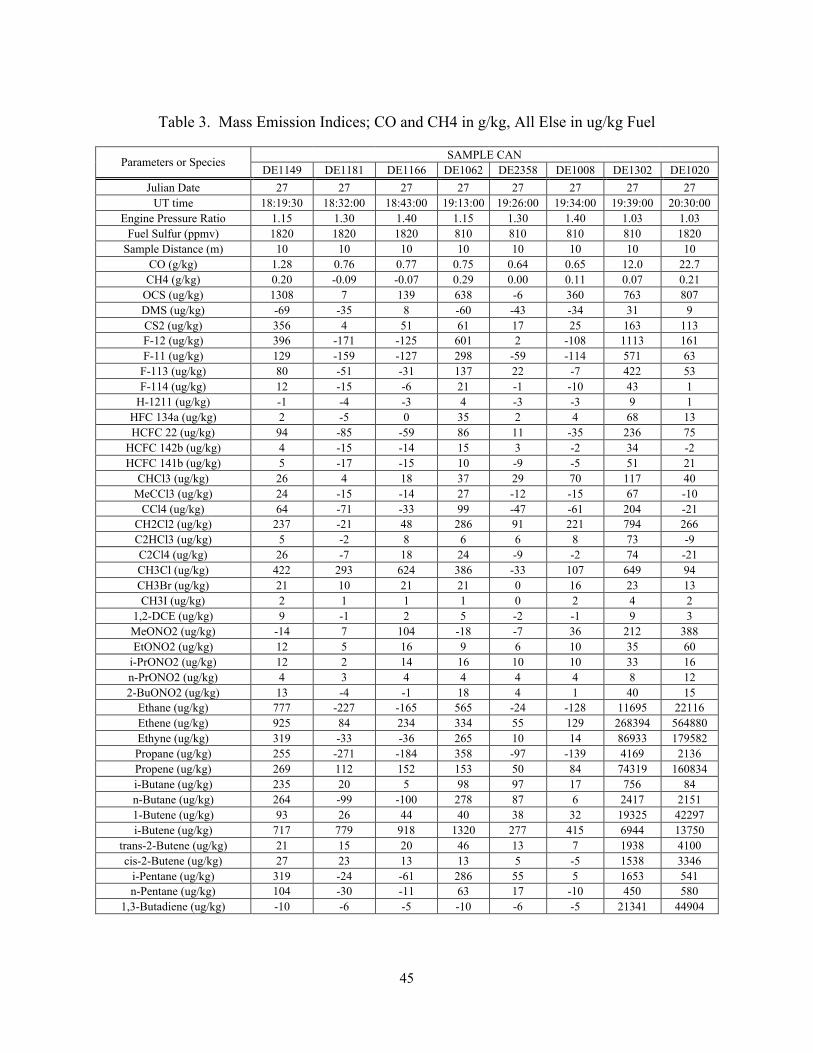
45

Table 3. Mass Emission Indices; CO and CH4 in g/kg, All Else in ug/kg Fuel

SAMPLE CANParameters or Species

DE1149 DE1181 DE1166 DE1062 DE2358 DE1008 DE1302 DE1020

Julian Date 27 27 27 27 27 27 27 27

UT time 18:19:30 18:32:00 18:43:00 19:13:00 19:26:00 19:34:00 19:39:00 20:30:00

Engine Pressure Ratio 1.15 1.30 1.40 1.15 1.30 1.40 1.03 1.03

Fuel Sulfur (ppmv) 1820 1820 1820 810 810 810 810 1820

Sample Distance (m) 10 10 10 10 10 10 10 10

CO (g/kg) 1.28 0.76 0.77 0.75 0.64 0.65 12.0 22.7

CH4 (g/kg) 0.20 -0.09 -0.07 0.29 0.00 0.11 0.07 0.21

OCS (ug/kg) 1308 7 139 638 -6 360 763 807

DMS (ug/kg) -69 -35 8 -60 -43 -34 31 9

CS2 (ug/kg) 356 4 51 61 17 25 163 113

F-12 (ug/kg) 396 -171 -125 601 2 -108 1113 161

F-11 (ug/kg) 129 -159 -127 298 -59 -114 571 63

F-113 (ug/kg) 80 -51 -31 137 22 -7 422 53

F-114 (ug/kg) 12 -15 -6 21 -1 -10 43 1

H-1211 (ug/kg) -1 -4 -3 4 -3 -3 9 1

HFC 134a (ug/kg) 2 -5 0 35 2 4 68 13

HCFC 22 (ug/kg) 94 -85 -59 86 11 -35 236 75

HCFC 142b (ug/kg) 4 -15 -14 15 3 -2 34 -2

HCFC 141b (ug/kg) 5 -17 -15 10 -9 -5 51 21

CHCl3 (ug/kg) 26 4 18 37 29 70 117 40

MeCCl3 (ug/kg) 24 -15 -14 27 -12 -15 67 -10

CCl4 (ug/kg) 64 -71 -33 99 -47 -61 204 -21

CH2Cl2 (ug/kg) 237 -21 48 286 91 221 794 266

C2HCl3 (ug/kg) 5 -2 8 6 6 8 73 -9

C2Cl4 (ug/kg) 26 -7 18 24 -9 -2 74 -21

CH3Cl (ug/kg) 422 293 624 386 -33 107 649 94

CH3Br (ug/kg) 21 10 21 21 0 16 23 13

CH3I (ug/kg) 2 1 1 1 0 2 4 2

1,2-DCE (ug/kg) 9 -1 2 5 -2 -1 9 3

MeONO2 (ug/kg) -14 7 104 -18 -7 36 212 388

EtONO2 (ug/kg) 12 5 16 9 6 10 35 60

i-PrONO2 (ug/kg) 12 2 14 16 10 10 33 16

n-PrONO2 (ug/kg) 4 3 4 4 4 4 8 12

2-BuONO2 (ug/kg) 13 -4 -1 18 4 1 40 15

Ethane (ug/kg) 777 -227 -165 565 -24 -128 11695 22116

Ethene (ug/kg) 925 84 234 334 55 129 268394 564880

Ethyne (ug/kg) 319 -33 -36 265 10 14 86933 179582

Propane (ug/kg) 255 -271 -184 358 -97 -139 4169 2136

Propene (ug/kg) 269 112 152 153 50 84 74319 160834

i-Butane (ug/kg) 235 20 5 98 97 17 756 84

n-Butane (ug/kg) 264 -99 -100 278 87 6 2417 2151

1-Butene (ug/kg) 93 26 44 40 38 32 19325 42297

i-Butene (ug/kg) 717 779 918 1320 277 415 6944 13750

trans-2-Butene (ug/kg) 21 15 20 46 13 7 1938 4100

cis-2-Butene (ug/kg) 27 23 13 13 5 -5 1538 3346

i-Pentane (ug/kg) 319 -24 -61 286 55 5 1653 541

n-Pentane (ug/kg) 104 -30 -11 63 17 -10 450 580

1,3-Butadiene (ug/kg) -10 -6 -5 -10 -6 -5 21341 44904

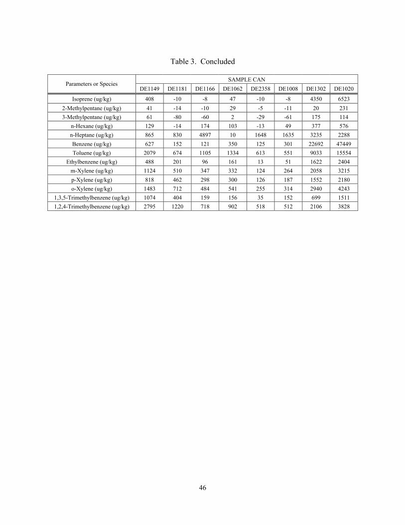
46

Table 3. Concluded

SAMPLE CANParameters or Species

DE1149 DE1181 DE1166 DE1062 DE2358 DE1008 DE1302 DE1020

Isoprene (ug/kg) 408 -10 -8 47 -10 -8 4350 6523

2-Methylpentane (ug/kg) 41 -14 -10 29 -5 -11 20 231

3-Methylpentane (ug/kg) 61 -80 -60 2 -29 -61 175 114

n-Hexane (ug/kg) 129 -14 174 103 -13 49 377 576

n-Heptane (ug/kg) 865 830 4897 10 1648 1635 3235 2288

Benzene (ug/kg) 627 152 121 350 125 301 22692 47449

Toluene (ug/kg) 2079 674 1105 1334 613 551 9033 15554

Ethylbenzene (ug/kg) 488 201 96 161 13 51 1622 2404

m-Xylene (ug/kg) 1124 510 347 332 124 264 2058 3215

p-Xylene (ug/kg) 818 462 298 300 126 187 1552 2180

o-Xylene (ug/kg) 1483 712 484 541 255 314 2940 4243

1,3,5-Trimethylbenzene (ug/kg) 1074 404 159 156 35 152 699 1511

1,2,4-Trimethylbenzene (ug/kg) 2795 1220 718 902 518 512 2106 3828

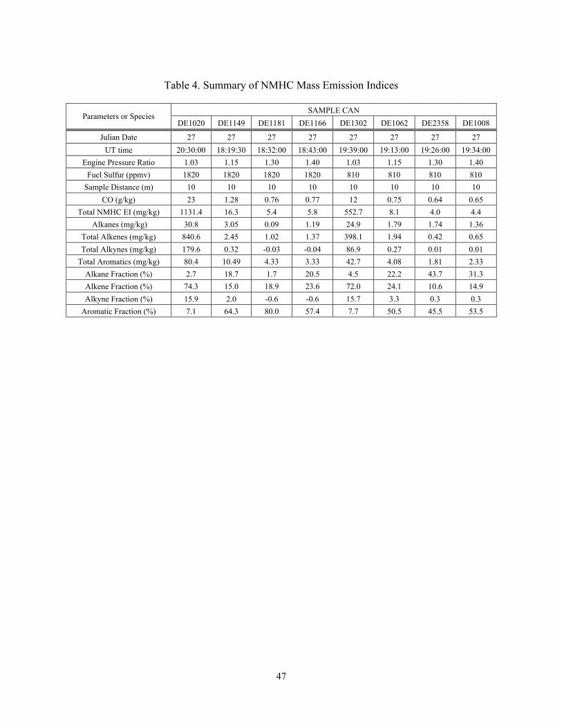
47

Table 4. Summary of NMHC Mass Emission Indices

SAMPLE CANParameters or Species

DE1020 DE1149 DE1181 DE1166 DE1302 DE1062 DE2358 DE1008

Julian Date 27 27 27 27 27 27 27 27

UT time 20:30:00 18:19:30 18:32:00 18:43:00 19:39:00 19:13:00 19:26:00 19:34:00

Engine Pressure Ratio 1.03 1.15 1.30 1.40 1.03 1.15 1.30 1.40

Fuel Sulfur (ppmv) 1820 1820 1820 1820 810 810 810 810

Sample Distance (m) 10 10 10 10 10 10 10 10

CO (g/kg) 23 1.28 0.76 0.77 12 0.75 0.64 0.65

Total NMHC EI (mg/kg) 1131.4 16.3 5.4 5.8 552.7 8.1 4.0 4.4

Alkanes (mg/kg) 30.8 3.05 0.09 1.19 24.9 1.79 1.74 1.36

Total Alkenes (mg/kg) 840.6 2.45 1.02 1.37 398.1 1.94 0.42 0.65

Total Alkynes (mg/kg) 179.6 0.32 -0.03 -0.04 86.9 0.27 0.01 0.01

Total Aromatics (mg/kg) 80.4 10.49 4.33 3.33 42.7 4.08 1.81 2.33

Alkane Fraction (%) 2.7 18.7 1.7 20.5 4.5 22.2 43.7 31.3

Alkene Fraction (%) 74.3 15.0 18.9 23.6 72.0 24.1 10.6 14.9

Alkyne Fraction (%) 15.9 2.0 -0.6 -0.6 15.7 3.3 0.3 0.3

Aromatic Fraction (%) 7.1 64.3 80.0 57.4 7.7 50.5 45.5 53.5

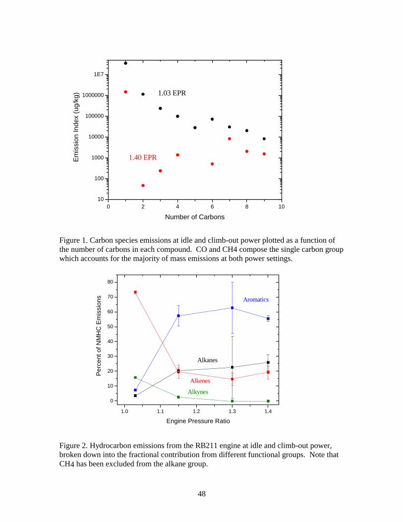
48

0 2 4 6 8 1010

100

1000

10000

100000

1000000

1E7

1.40 EPR

1.03 EPR

Em

issi

on In

dex

(ug/

kg)

Number of Carbons

Figure 1. Carbon species emissions at idle and climb-out power plotted as a function of the number of carbons in each compound. CO and CH4 compose the single carbon group which accounts for the majority of mass emissions at both power settings.

1.0 1.1 1.2 1.3 1.4

0

10

20

30

40

50

60

70

80

Aromatics

Alkynes

Alkenes

Alkanes

Per

cent

of N

MH

C E

mis

sion

s

Engine Pressure Ratio

Figure 2. Hydrocarbon emissions from the RB211 engine at idle and climb-out power, broken down into the fractional contribution from different functional groups. Note that CH4 has been excluded from the alkane group.

49

1.00 1.05 1.10 1.15 1.20 1.25 1.30 1.35 1.40 1.45

0.01

0.1

1

10

NMHC

CO

Em

issi

on In

dex

(g/k

g)

Engine Pressure Ratio

Figure 3. CO and total NMHC emission indices as a function of engine power where 1.03 EPR is idle and 1.4 is equivalent to climb-out.

1 10

10

100

1000

NM

HC

Em

issi

on In

dex

(mg/

kg)

CO Emision Index (g/kg)

Figure 4. Total NMHC EI’s plotted as a function of CO EI.

50

APPENDIX C: ARI-RR-1362 ARI Contract # 10154 NASA Contract # C76653N

TECHNICAL SUPPORT OF MEASUREMENTS OF SO2, SO3, HONO, CO2

Final Report for Task 2 of Contract C7665N

Prepared by

J. Wormhoudt and R. Miake-Lye Aerodyne Research, Inc.

45 Manning Road Billerica, MA 01821-3976

Prepared for

Dr. Chowen Wey Aeropropulsion and Information Technology Branch

NASA Glenn Research Center 21000 Brookpark Road

Cleveland, OH 44135-3191

June 2003

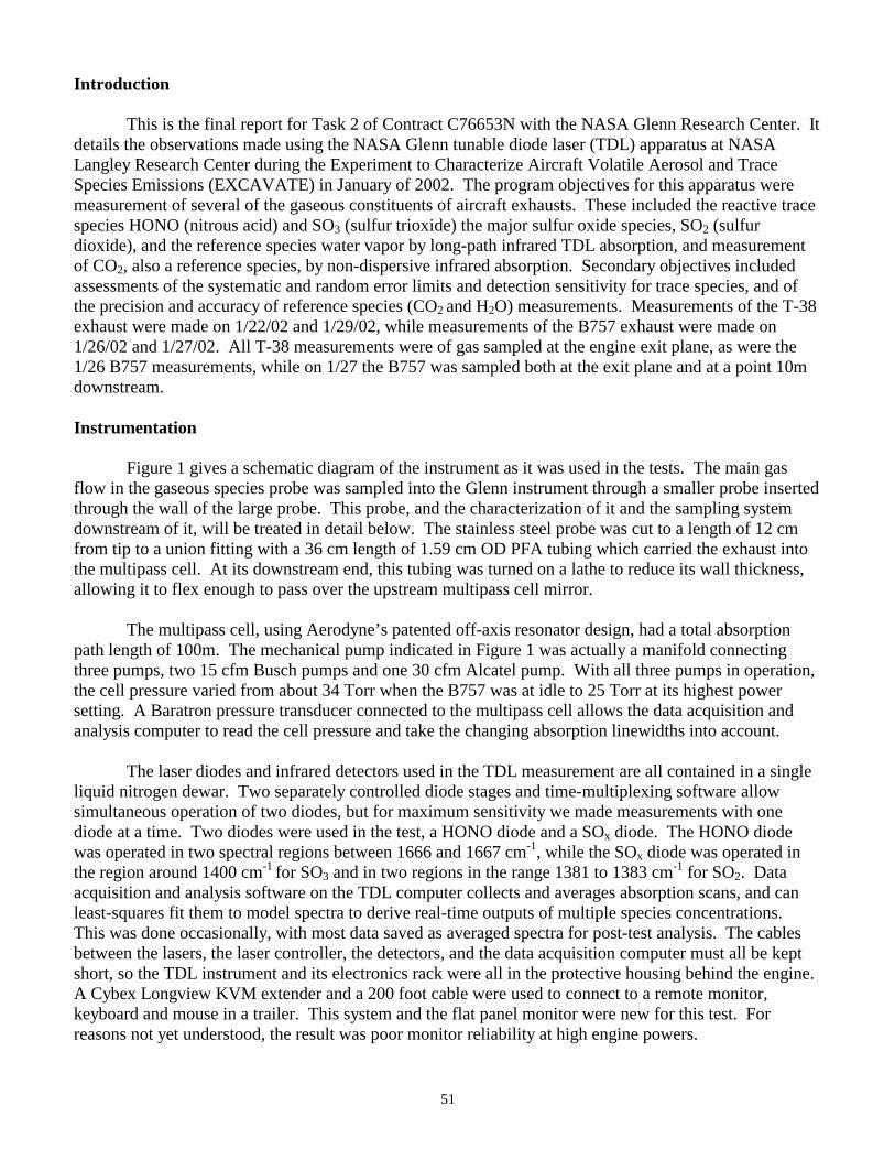
51

Introduction This is the final report for Task 2 of Contract C76653N with the NASA Glenn Research Center. It details the observations made using the NASA Glenn tunable diode laser (TDL) apparatus at NASA Langley Research Center during the Experiment to Characterize Aircraft Volatile Aerosol and Trace Species Emissions (EXCAVATE) in January of 2002. The program objectives for this apparatus were measurement of several of the gaseous constituents of aircraft exhausts. These included the reactive trace species HONO (nitrous acid) and SO3 (sulfur trioxide) the major sulfur oxide species, SO2 (sulfur dioxide), and the reference species water vapor by long-path infrared TDL absorption, and measurement of CO2, also a reference species, by non-dispersive infrared absorption. Secondary objectives included assessments of the systematic and random error limits and detection sensitivity for trace species, and of the precision and accuracy of reference species (CO2 and H2O) measurements. Measurements of the T-38 exhaust were made on 1/22/02 and 1/29/02, while measurements of the B757 exhaust were made on 1/26/02 and 1/27/02. All T-38 measurements were of gas sampled at the engine exit plane, as were the 1/26 B757 measurements, while on 1/27 the B757 was sampled both at the exit plane and at a point 10m downstream. Instrumentation Figure 1 gives a schematic diagram of the instrument as it was used in the tests. The main gas flow in the gaseous species probe was sampled into the Glenn instrument through a smaller probe inserted through the wall of the large probe. This probe, and the characterization of it and the sampling system downstream of it, will be treated in detail below. The stainless steel probe was cut to a length of 12 cm from tip to a union fitting with a 36 cm length of 1.59 cm OD PFA tubing which carried the exhaust into the multipass cell. At its downstream end, this tubing was turned on a lathe to reduce its wall thickness, allowing it to flex enough to pass over the upstream multipass cell mirror.

The multipass cell, using Aerodyne’s patented off-axis resonator design, had a total absorption path length of 100m. The mechanical pump indicated in Figure 1 was actually a manifold connecting three pumps, two 15 cfm Busch pumps and one 30 cfm Alcatel pump. With all three pumps in operation, the cell pressure varied from about 34 Torr when the B757 was at idle to 25 Torr at its highest power setting. A Baratron pressure transducer connected to the multipass cell allows the data acquisition and analysis computer to read the cell pressure and take the changing absorption linewidths into account. The laser diodes and infrared detectors used in the TDL measurement are all contained in a single liquid nitrogen dewar. Two separately controlled diode stages and time-multiplexing software allow simultaneous operation of two diodes, but for maximum sensitivity we made measurements with one diode at a time. Two diodes were used in the test, a HONO diode and a SOx diode. The HONO diode was operated in two spectral regions between 1666 and 1667 cm-1, while the SOx diode was operated in the region around 1400 cm-1 for SO3 and in two regions in the range 1381 to 1383 cm-1 for SO2. Data acquisition and analysis software on the TDL computer collects and averages absorption scans, and can least-squares fit them to model spectra to derive real-time outputs of multiple species concentrations. This was done occasionally, with most data saved as averaged spectra for post-test analysis. The cables between the lasers, the laser controller, the detectors, and the data acquisition computer must all be kept short, so the TDL instrument and its electronics rack were all in the protective housing behind the engine. A Cybex Longview KVM extender and a 200 foot cable were used to connect to a remote monitor, keyboard and mouse in a trailer. This system and the flat panel monitor were new for this test. For reasons not yet understood, the result was poor monitor reliability at high engine powers.

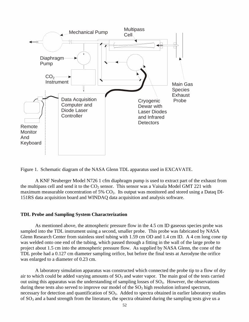
52

Figure 1. Schematic diagram of the NASA Glenn TDL apparatus used in EXCAVATE. A KNF Neuberger Model N726 1 cfm diaphragm pump is used to extract part of the exhaust from the multipass cell and send it to the CO2 sensor. This sensor was a Vaisala Model GMT 221 with maximum measurable concentration of 5% CO2. Its output was monitored and stored using a Dataq DI-151RS data acquisition board and WINDAQ data acquisition and analysis software. TDL Probe and Sampling System Characterization

As mentioned above, the atmospheric pressure flow in the 4.5 cm ID gaseous species probe was sampled into the TDL instrument using a second, smaller probe. This probe was fabricated by NASA Glenn Research Center from stainless steel tubing with 1.59 cm OD and 1.4 cm ID. A 4 cm long cone tip was welded onto one end of the tubing, which passed through a fitting in the wall of the large probe to project about 1.5 cm into the atmospheric pressure flow. As supplied by NASA Glenn, the cone of the TDL probe had a 0.127 cm diameter sampling orifice, but before the final tests at Aerodyne the orifice was enlarged to a diameter of 0.23 cm.

A laboratory simulation apparatus was constructed which connected the probe tip to a flow of dry

air to which could be added varying amounts of SO3 and water vapor. The main goal of the tests carried out using this apparatus was the understanding of sampling losses of SO3. However, the observations during these tests also served to improve our model of the SO3 high resolution infrared spectrum, necessary for detection and quantification of SO3. Added to spectra obtained in earlier laboratory studies of SO3 and a band strength from the literature, the spectra obtained during the sampling tests give us a

MultipassCell

CryogenicDewar withLaser Diodesand InfraredDetectors

DiaphragmPump

COInstrument

2

Mechanical Pump

Main GasSpeciesExhaust ProbeData Acquisition

Computer andDiode LaserController

RemoteMonitorAnd Keyboard

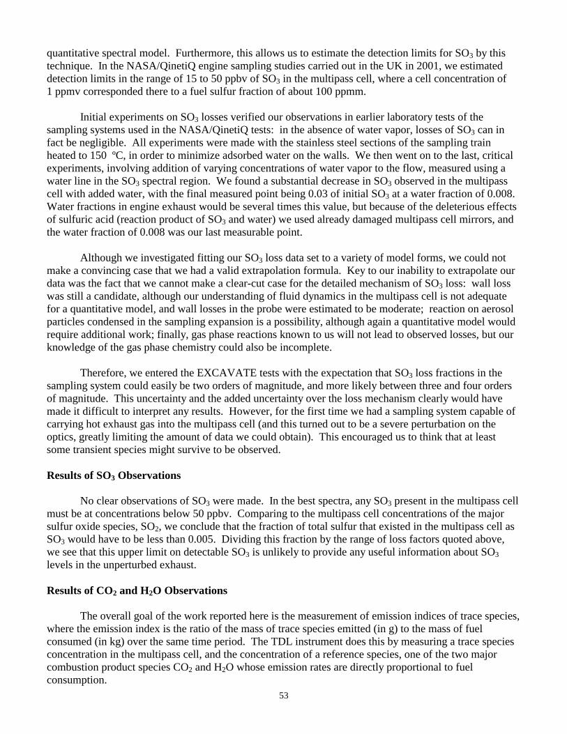
53

quantitative spectral model. Furthermore, this allows us to estimate the detection limits for SO3 by this technique. In the NASA/QinetiQ engine sampling studies carried out in the UK in 2001, we estimated detection limits in the range of 15 to 50 ppbv of SO3 in the multipass cell, where a cell concentration of 1 ppmv corresponded there to a fuel sulfur fraction of about 100 ppmm. Initial experiments on SO3 losses verified our observations in earlier laboratory tests of the sampling systems used in the NASA/QinetiQ tests: in the absence of water vapor, losses of SO3 can in fact be negligible. All experiments were made with the stainless steel sections of the sampling train heated to 150 ºC, in order to minimize adsorbed water on the walls. We then went on to the last, critical experiments, involving addition of varying concentrations of water vapor to the flow, measured using a water line in the SO3 spectral region. We found a substantial decrease in SO3 observed in the multipass cell with added water, with the final measured point being 0.03 of initial SO3 at a water fraction of 0.008. Water fractions in engine exhaust would be several times this value, but because of the deleterious effects of sulfuric acid (reaction product of SO3 and water) we used already damaged multipass cell mirrors, and the water fraction of 0.008 was our last measurable point.

Although we investigated fitting our SO3 loss data set to a variety of model forms, we could not

make a convincing case that we had a valid extrapolation formula. Key to our inability to extrapolate our data was the fact that we cannot make a clear-cut case for the detailed mechanism of SO3 loss: wall loss was still a candidate, although our understanding of fluid dynamics in the multipass cell is not adequate for a quantitative model, and wall losses in the probe were estimated to be moderate; reaction on aerosol particles condensed in the sampling expansion is a possibility, although again a quantitative model would require additional work; finally, gas phase reactions known to us will not lead to observed losses, but our knowledge of the gas phase chemistry could also be incomplete.

Therefore, we entered the EXCAVATE tests with the expectation that SO3 loss fractions in the

sampling system could easily be two orders of magnitude, and more likely between three and four orders of magnitude. This uncertainty and the added uncertainty over the loss mechanism clearly would have made it difficult to interpret any results. However, for the first time we had a sampling system capable of carrying hot exhaust gas into the multipass cell (and this turned out to be a severe perturbation on the optics, greatly limiting the amount of data we could obtain). This encouraged us to think that at least some transient species might survive to be observed. Results of SO3 Observations No clear observations of SO3 were made. In the best spectra, any SO3 present in the multipass cell must be at concentrations below 50 ppbv. Comparing to the multipass cell concentrations of the major sulfur oxide species, SO2, we conclude that the fraction of total sulfur that existed in the multipass cell as SO3 would have to be less than 0.005. Dividing this fraction by the range of loss factors quoted above, we see that this upper limit on detectable SO3 is unlikely to provide any useful information about SO3 levels in the unperturbed exhaust. Results of CO2 and H2O Observations The overall goal of the work reported here is the measurement of emission indices of trace species, where the emission index is the ratio of the mass of trace species emitted (in g) to the mass of fuel consumed (in kg) over the same time period. The TDL instrument does this by measuring a trace species concentration in the multipass cell, and the concentration of a reference species, one of the two major combustion product species CO2 and H2O whose emission rates are directly proportional to fuel consumption.

54

H2O lines appear in each of the spectral regions described above for the various trace gases, and

thus water vapor concentrations can be measured “for free” with every trace species measurement. However, each spectral region is selected so that the strengths and positions of the trace species lines will be optimal for sensitive and accurate detection, and the result is that the coincidental water lines are not optimal for accurate measurement. In the EXCAVATE data set we found the same situation as in earlier tests: the H2O concentration data sets extracted from TDL spectra both had larger variances and larger systematic errors than the CO2 data sets. In addition, use of H2O as the reference species means that accurate values of inlet air humidity must be obtained and subtracted from the TDL observations to give the H2O derived from the fuel. Although we had thought that humidity values would be available from the local weather observation station, we have so far been unable to retrieve these records for several of the test days. Therefore, we will not discuss the H2O data set in detail here, but go on to the CO2 data measured by the Vaisala instrument monitoring the NASA Glenn multipass cell exhaust, and compare it to CO2 measurements made by NASA LaRC.

A representation of these data sets is given in the plots in Figures 2 through 4. Figure 2 presents a

critical selection of the measurements made during the two T-38 test days observed by the NASA Glenn instrument. Figure 3 summarizes observations made at the B757 exit plane, while Figure 4 does the same for observations made 10m behind the B757 engine. In all cases, error bars represent the standard deviations in multiple measurements, and when there is no error bar, only one measurement is involved.

It can be seen that the NASA Glenn and NASA LaRC measurements often agree to within the

error bars, though not always. In general, there are reasons to prefer the NASA Glenn values for the 1/22 test, and to prefer the NASA LaRC values for the other three days. (In the comparison plots, the good values from each instruments are used, so some comparisons are for the same conditions but between different days.) We have concluded, after detailed analysis, that the two data sets taken together allow us to deduce a reliable value of CO2 concentration for every set of engine and sampling parameters.

Figure 2. Best values for T-38 exhaust CO2 concentrations from NASA Glenn and NASA LaRC.

4

3

2

1

0

Per

Cen

t by

Vol

ume

50 60 70 80 90 100

Power Setting

GRC CO2 LaRC CO2

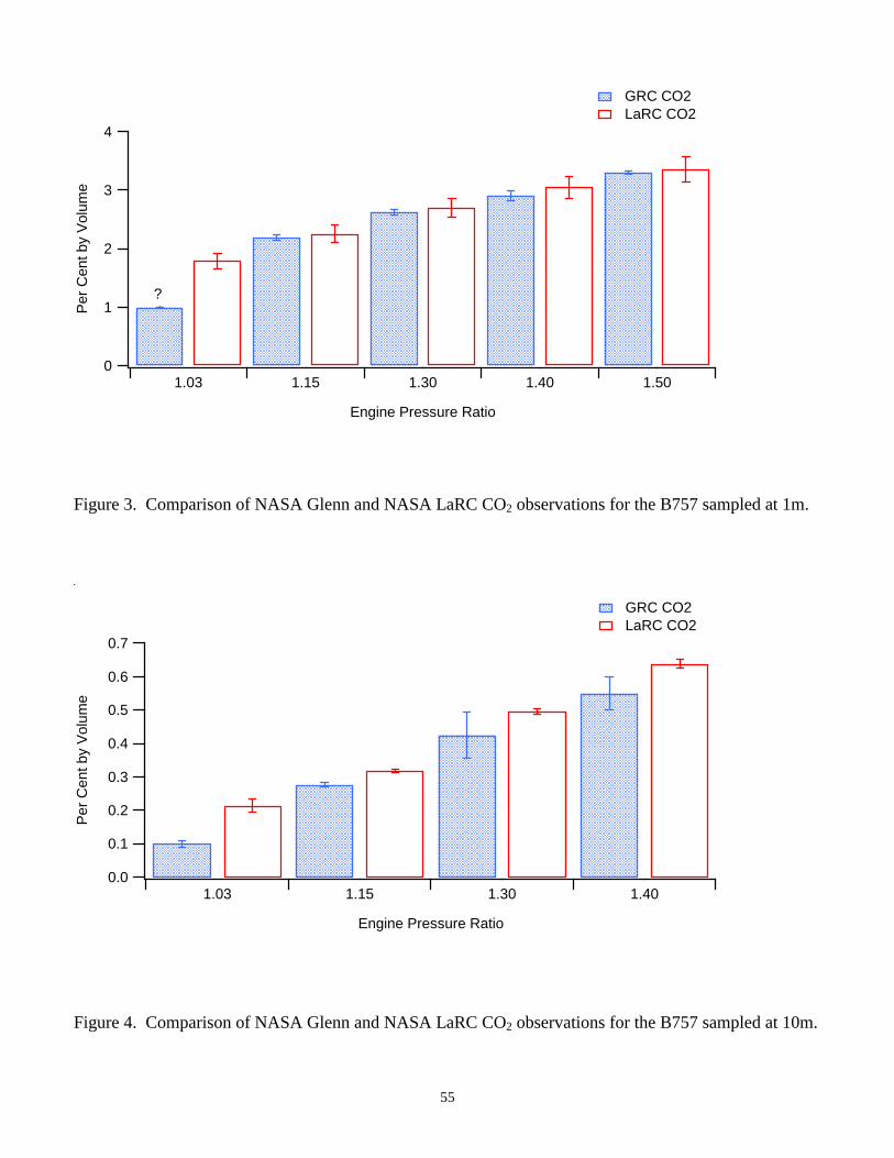
55

Figure 3. Comparison of NASA Glenn and NASA LaRC CO2 observations for the B757 sampled at 1m.

Figure 4. Comparison of NASA Glenn and NASA LaRC CO2 observations for the B757 sampled at 10m.

4

3

2

1

0

Per

Cen

t by

Vol

ume

1.03 1.15 1.30 1.40 1.50

Engine Pressure Ratio

GRC CO2 LaRC CO2

?

0.7

0.6

0.5

0.4

0.3

0.2

0.1

0.0

Per

Cen

t by

Vol

ume

1.03 1.15 1.30 1.40

Engine Pressure Ratio

GRC CO2 LaRC CO2

56

Results of SO2 Observations Since SO2 is the overwhelmingly predominant sulfur oxide species, and since its only source is the sulfur contained in the fuel, measurements of SO2 emission indices are constrained in a way that those of NOx, for example, are not. That is, the SO2 emission index, or g SO2 per kg of fuel, is directly related to the fuel sulfur fraction, or g S per g of fuel. In fact, in presenting our results, we will simply make that conversion and then, when fuel sulfur analyses are available, take the ratio and report SO2 as a fraction of total fuel sulfur. A fraction of fuel sulfur in SO2 that is significantly less than one could indicate that some other sulfur oxide species was present in the exhaust, but a fraction that is greater than one is simply an indication of systematic errors in measurements of SO2 and/or CO2 concentrations. In the T-38 tests, measurements of SO2 expressed as fuel sulfur fraction were obtained for the 50, 70 and 90 per cent power settings. For the first two settings the value obtained was 1665 ppmm, while for the 90 per cent power setting it was 1440 ppmm. When we take into account the roughly 20 per cent error bars we expect from the combination of systematic and random errors, these two values are not significantly different. At present we do not have a sulfur analysis for the T-38 fuel, so we cannot comment further on these results. Figures 5 and 6 present results of SO2 measurements of the B757 exhaust at the two measurement positions. SO2 emission index fractional standard deviations in multiple measurements were typically less than 10 per cent. The analysis of systematic as well as random errors detailed in previous reports leads to total error estimates of 20 per cent or more. By this standard, all points in Figure 5 and all but one or two in Figure 6 show the TDL measured SO2 to agree with the total fuel sulfur from the LaRC fuel analyses. The values in Figure 5 lie in the range of 0.75 to 1.0, while those in Figure 6 are distributed evenly above and below a ratio of 1. Table 1 lists the SO2 emission index values used to prepare the figures.

Figure 5. SO2 measurements at 1m behind the B757, expressed as fraction of fuel sulfur.

1.6

1.4

1.2

1.0

0.8

0.6

0.4

0.2

0.0

Fra

ctio

n of

Sul

fur

in S

O2

1.51.41.31.21.11.0

EPR

810 ppmm S in fuel 1050 ppmm S in fuel 1820 ppmm S in fuel

Sampling B757 at 1m

57

The measurements in Figure 6 taken at 10m represent a less stressful environment but lower

concentrations of SO2, which could lead to a noisier data set. There is indeed a larger spread in the ratios in Figure 6. This makes it difficult to be sure that the apparent trend, of decreasing fraction in SO2 with increasing power, is real. This trend is at least consistent with an additional data set, in which automatic fitting of the SO2 spectra was used to write a real-time record of SO2 and water concentrations, a so-called “streaming file”. In a period of less than an hour, the B757 power was varied from 1.03 pressure ratio through the two intermediate settings all the way to 1.40, then returned to 1.03 (idle). Each increase in power showed a clear decrease in SO2 fraction, outside of the range of variation, with the total change from 1.03 to 1.40 being about 30%, and the final return to 1.03 coincided with a return to the original high value of SO2. At this point, we simply note this as a possible systematic problem in the 10m sampling, although we cannot suggest a mechanism for an actual change in plume chemistry.

Figure 6. SO2 measurements at 10m behind the B757, expressed as fraction of fuel sulfur. Table 1. TDL measured SO2 emission index values (as ppmv in fuel) for B757 exhaust sampling. At 1m: Fuel Sulfur. EI(SO2), At 10m: Fuel Sulfur, EI(SO2), EPR Run ppmv ppmv EPR Run ppmv ppmv 1.03 92 810 680 1.03 102,103 1050 1490 1.03 28,30 1050 1040 1.03 115,138,149 1820 1980 1.03 42,60 1820 1410 1.15 132-132 810 1045 1.15 31 1050 1020 1.15 105-107 1050 940 1.15 46,65 1820 1580 1.15 141 1820 2110 1.30 82 1050 680 1.30 121,144-146 1820 1575 1.40 136-137 810 870 1.40 147-148 1820 1810

1.6

1.4

1.2

1.0

0.8

0.6

0.4

0.2

0.0

Fra

ctio

n of

Sul

fur

in S

O2

1.51.41.31.21.11.0

EPR

810 ppmm S in fuel 1050 ppmm S in fuel 1820 ppmm S in fuel

Sampling B757 at 10m

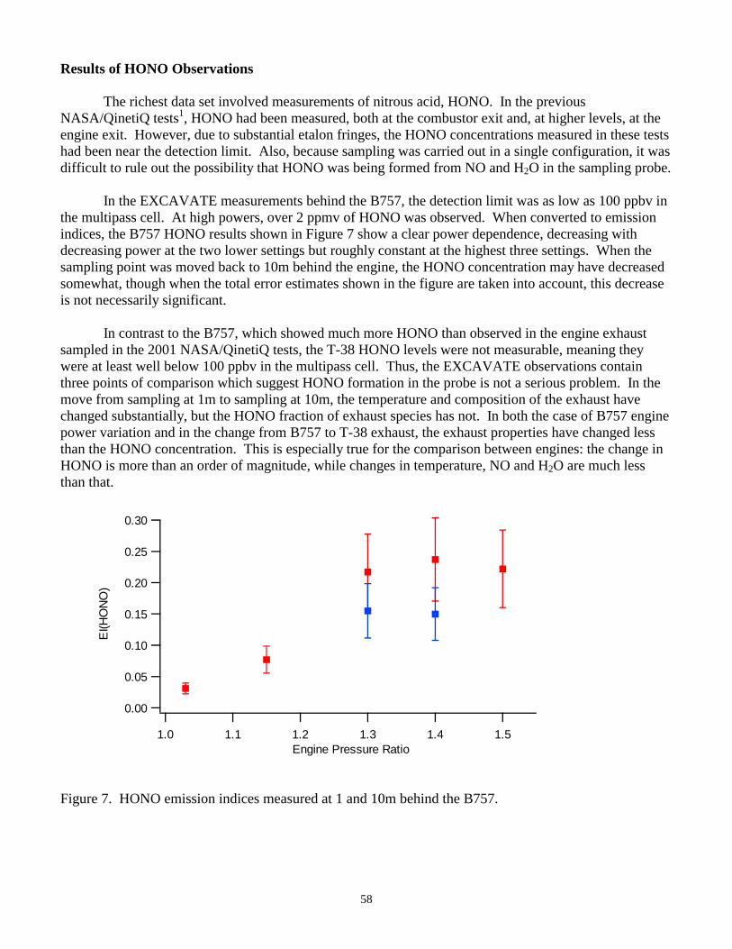
58

Results of HONO Observations The richest data set involved measurements of nitrous acid, HONO. In the previous NASA/QinetiQ tests1, HONO had been measured, both at the combustor exit and, at higher levels, at the engine exit. However, due to substantial etalon fringes, the HONO concentrations measured in these tests had been near the detection limit. Also, because sampling was carried out in a single configuration, it was difficult to rule out the possibility that HONO was being formed from NO and H2O in the sampling probe. In the EXCAVATE measurements behind the B757, the detection limit was as low as 100 ppbv in the multipass cell. At high powers, over 2 ppmv of HONO was observed. When converted to emission indices, the B757 HONO results shown in Figure 7 show a clear power dependence, decreasing with decreasing power at the two lower settings but roughly constant at the highest three settings. When the sampling point was moved back to 10m behind the engine, the HONO concentration may have decreased somewhat, though when the total error estimates shown in the figure are taken into account, this decrease is not necessarily significant. In contrast to the B757, which showed much more HONO than observed in the engine exhaust sampled in the 2001 NASA/QinetiQ tests, the T-38 HONO levels were not measurable, meaning they were at least well below 100 ppbv in the multipass cell. Thus, the EXCAVATE observations contain three points of comparison which suggest HONO formation in the probe is not a serious problem. In the move from sampling at 1m to sampling at 10m, the temperature and composition of the exhaust have changed substantially, but the HONO fraction of exhaust species has not. In both the case of B757 engine power variation and in the change from B757 to T-38 exhaust, the exhaust properties have changed less than the HONO concentration. This is especially true for the comparison between engines: the change in HONO is more than an order of magnitude, while changes in temperature, NO and H2O are much less than that.

Figure 7. HONO emission indices measured at 1 and 10m behind the B757.

0.30

0.25

0.20

0.15

0.10

0.05

0.00

EI(H

ON

O)

1.51.41.31.21.11.0Engine Pressure Ratio

59

Summary

In summary, several points can be made about the data taken by the NASA Glenn TDL instrument at EXCAVATE. Analysis of the CO2 data taken by the Vaisala instrument which sampled the TDL instrument’s exhaust, and the CO2 data taken by NASA LaRC should give a reliable value for each value of engine and sampling parameters.

The detection limit for SO3 in the multipass cell less than 50 ppbv. However, SO3 was not observed, with an upper limit for SO3 as a fraction of total sulfur in cell being less than 0.005. Because we expected sampling losses of at least two orders of magnitude, and more likely between three and four orders of magnitude, this upper limit most likely does not provide any useful information about the level of SO3 in the exhaust. Multiple measurements of SO2 showed good repeatability, with SO2 emission index fractional standard deviations typically less than 10 per cent. For the B757 measured at 1m, the EI(SO2) values derived from TDL measurements of SO2 and NASA LaRC measurements of CO2 were not significantly different from the total exhaust sulfur emission index derived from the NASA LaRC fuel analyses. For the B757 measured at 10m, where the EI(SO2) values are more scattered, there may be a trend of decreasing fraction in SO2 with increasing power, but the scatter in the data does not allow us to conclude that this is a real trend.

The TDL detection limit for HONO was as low as 100 ppbv. At high power, over 2 ppmv of HONO was detected in the B757 exhaust. These values correspond to EI(HONO) values of up to 0.25 (if nominal values apply to this exhaust, this is somewhat less than 5% of the NO). By contrast, HONO was not detected in the T-38 exhaust. HONO variation with a change in sampling position in the B757 exhaust from 1m to 10m was not significant. Changes with B757 power setting, on the other hand, were clearly seen, with the lower two power settings yielding significantly lower emission indices than the higher settings. All of these trends confirm earlier HONO observations, and argue against the possibility that significant HONO is formed in the sampling line. References 1. “QinetiQ/NASA Collaborative Programme – Final Report,” produced for UK Department of Trade

and Industry Under Order/Contract reference F11X1DXX by QinetiQ Ltd, Cody Technology Park, Farnborough, Hampshire GU14 0LX, UK.

60

APPENDIX D: Concentrations and Physical Properties of Jet Engine Exhaust Aerosols Sampled during EXCAVATE

Bruce E. Anderson, Edward L. Winstead, Charles H. Hudgins, James V. Plant, H.-S.

Branham, and K. Lee Thornhill

NASA Langley Research Center Hampton VA 23662

1.0 Background Aircraft are prolific sources of both primary and secondary aerosol particles (i.e., Friedl et al., 1997). Composed of soot and perhaps condensed organic carbon and sulfur species, these particles can potentially impact climate by influencing a number of important atmospheric processes including radiation transfer; cloud formation, duration, and albedo; and heterogeneous chemical reaction rates. In addition, release of such particles in airport terminal areas can have deleterious health effects upon exposed workers as well as reduce local air quality and visibility. To quantify and better understand the generation of particulates and pollutants by aircraft, the National Aeronautics and Space Administration (NASA), through its Atmospheric Effects of Aviation Project, has sponsored several cooperative field investigations, the latest of which was the Experiment to Characterize Aircraft Volatile Aerosol and Trace Species Emissions or EXCAVATE. Conducted at NASA LaRC during January 2002, EXCAVATE was designed to address a number of particle-related objectives, including quantifying and characterizing turbine engine black carbon and nonvolatile particle emissions as well as investigating the formation and growth of volatile particles in the plume as a function of plume age, fuel S content, and engine power. The experiment included sampling exhaust emissions from the J85-GE and a RB-211 engines on the LaRC T-38A and B-757 aircraft, respectively, as they were operated in a ground-based run-up facility. The LaRC In Situ Measurements Group participated in EXCAVATE and played a key role in addressing project objectives by providing a suite of instruments to measure particle number density as a function of size diameter and aerosol absorption coefficients from which black carbon mass is inferred. The text below provides a description of the LaRC instrument package and sampling procedures and a summary of observations. 2.0 Experiment Figure 1 shows a diagram of the LaRC aerosol characterization system. Important components include 1) a TSI 3022 condensation nuclei counter (CNC) to measure total aerosol number density; 2) a pair of TSI 3760 CNCs to determine the fraction of particles >12 nm that are volatile at temperatures below 300 oC; 3) a dual, differential mobility analyzer (dDMA) to provide 60-second resolution, particle size distributions over the 0.004 to 0.240 µm diameter range; 4) an optical particle counter to measure aerosol size

61

distributions in the 0.1 to 1 µm range; and 5) a particle soot absorption photometer (PSAP) for total aerosol absorption (i.e., carbon black) measurements. The specific parameters measured by these instruments along with their anticipated precisions and accuracies are listed in Table 1; brief descriptions are provided below. Total aerosol concentrations were monitored with a TSI3022 CNC because, unlike the single particle counting units like the TSI3025 and 3760, it has a photometric, ensemble sampling mode that extends its dynamic range to >107 cm-3. This is particularly important because the exhaust samples often contained >10-6 cm-3 particles, even after a 10-fold dilution. This CNC has a 50 percent cut size of ~7 nm at sea level pressure and a response time of < 5 seconds. Cofer et al., (1999) describes the identical CNCs (TSI3760 CNCs) that were used to determine the fractional volatility of aerosol samples and discusses their calibration and performance at subambient pressures. These instruments provided a means for distinguishing soot from condensed hydrocarbon and sulfate particles, but, unfortunately, their upper concentration range is ~2 x 104 cm-3, so their signals were often saturated when sampling the highly concentrated exhaust plumes. The dual differential mobility analyzer (dDMA) used to record nucleation and accumulation mode size distributions was composed of a TSI nano-DMA column (nDMA) and a TSI long-DMA column (lDMA), both connected to the same voltage sweep generator and input particle neutralizer. Output from the nDMA was routed to a TSI 3025 CNC, whereas the lDMA was connected to a TSI 3762. Both systems provided 25 channels of logarithmically spaced sizing data, the nDMA over the range for 3 to 85 nm and the lDMA from 9 to 240 nm. The particle transfer functions for the DMAs were determined for 500 Torr operation and were applied to the voltage sweeps to obtain size distributions appropriate for the pressure and temperature of operation. Size distributions were derived using the technique described by Wang and Flagan (1990) and the accuracy of the inversions were verified by comparing integrated number densities to those recorded by a CNC that continuously monitored number densities in the sample stream. Size scans recorded during times when concentrations changed by more than 50 percent were rejected as bad data. The two DMAs were operated in overlap mode (i.e., both sampled the same input stream) while sampling the B-757 to provide improved resolution and counting efficiency for nucleation mode particles; however, an inline heater was placed on the input of the lDMA on the last set of T-38 engine runs to allow us to distinguish the portion of the observed aerosol size distribution that could be attributed to soot from that related to condensed hydrocarbons and sulfates. Aerosol size in the 0.1 to 1 um size range was determined using a Particle Measuring Systems (PMS), High Sensitivity Laser Aerosol Spectrometer (HSLAS). Based on Mie scattering principle, this instrument sizes particles by measuring the hemispheric side-scatter from particles passing through feedback cavity of a 683 nm helium-neon laser. The instrument provides 30 bins of size data that are updated continuously. It was calibrated for size sensitivity using latex spheres and for concentration by comparison to a CNC for measuring the number density of monodisperse particles output by a DMA.

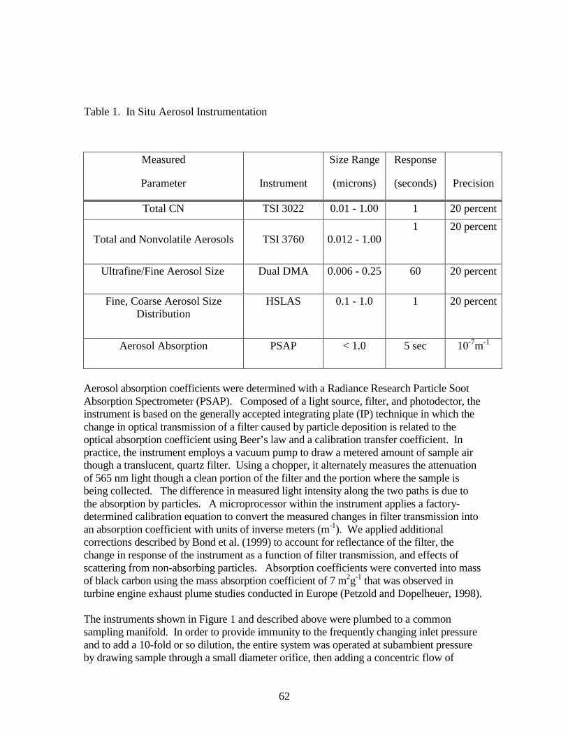
62

Table 1. In Situ Aerosol Instrumentation

Measured Size Range Response

Parameter Instrument (microns) (seconds) Precision

Total CN TSI 3022 0.01 - 1.00 1 20 percent

Total and Nonvolatile Aerosols

TSI 3760

0.012 - 1.00

1 20 percent

Ultrafine/Fine Aerosol Size Dual DMA 0.006 - 0.25 60 20 percent

Fine, Coarse Aerosol Size Distribution

HSLAS 0.1 - 1.0 1 20 percent

Aerosol Absorption PSAP < 1.0 5 sec 10-7m-1

Aerosol absorption coefficients were determined with a Radiance Research Particle Soot Absorption Spectrometer (PSAP). Composed of a light source, filter, and photodector, the instrument is based on the generally accepted integrating plate (IP) technique in which the change in optical transmission of a filter caused by particle deposition is related to the optical absorption coefficient using Beer’s law and a calibration transfer coefficient. In practice, the instrument employs a vacuum pump to draw a metered amount of sample air though a translucent, quartz filter. Using a chopper, it alternately measures the attenuation of 565 nm light though a clean portion of the filter and the portion where the sample is being collected. The difference in measured light intensity along the two paths is due to the absorption by particles. A microprocessor within the instrument applies a factory-determined calibration equation to convert the measured changes in filter transmission into an absorption coefficient with units of inverse meters (m-1). We applied additional corrections described by Bond et al. (1999) to account for reflectance of the filter, the change in response of the instrument as a function of filter transmission, and effects of scattering from non-absorbing particles. Absorption coefficients were converted into mass of black carbon using the mass absorption coefficient of 7 m2g-1 that was observed in turbine engine exhaust plume studies conducted in Europe (Petzold and Dopelheuer, 1998). The instruments shown in Figure 1 and described above were plumbed to a common sampling manifold. In order to provide immunity to the frequently changing inlet pressure and to add a 10-fold or so dilution, the entire system was operated at subambient pressure by drawing sample through a small diameter orifice, then adding a concentric flow of

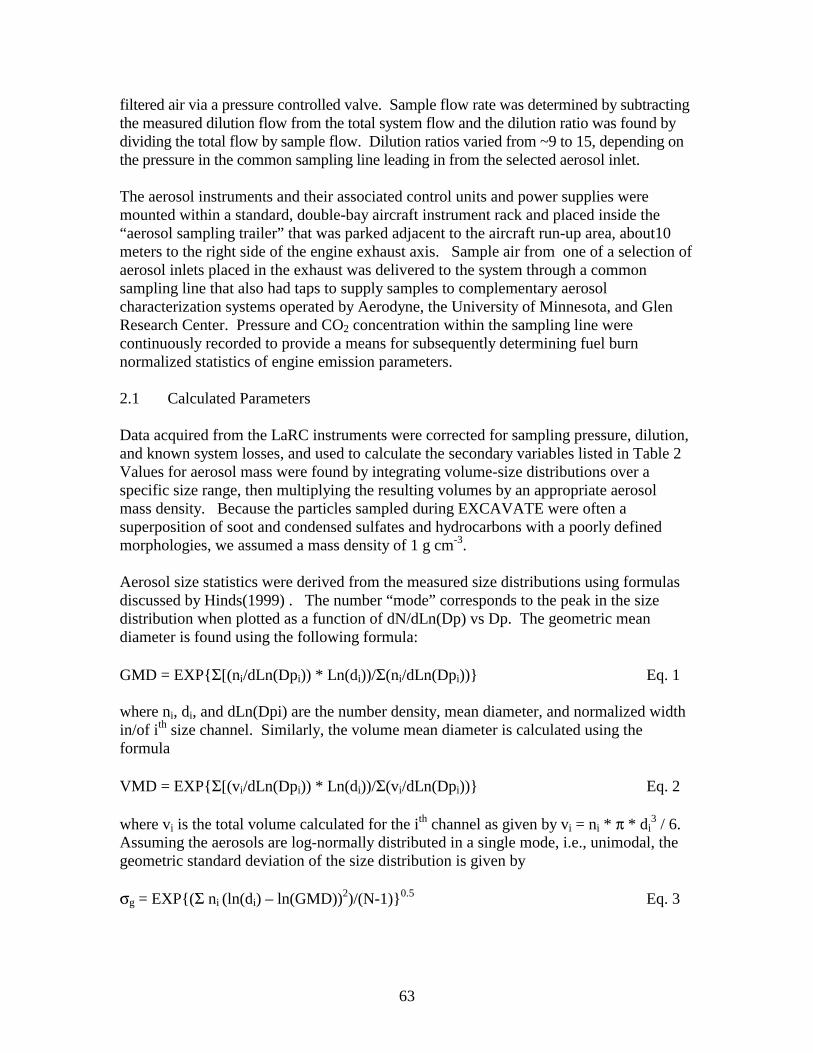
63

filtered air via a pressure controlled valve. Sample flow rate was determined by subtracting the measured dilution flow from the total system flow and the dilution ratio was found by dividing the total flow by sample flow. Dilution ratios varied from ~9 to 15, depending on the pressure in the common sampling line leading in from the selected aerosol inlet. The aerosol instruments and their associated control units and power supplies were mounted within a standard, double-bay aircraft instrument rack and placed inside the “aerosol sampling trailer” that was parked adjacent to the aircraft run-up area, about10 meters to the right side of the engine exhaust axis. Sample air from one of a selection of aerosol inlets placed in the exhaust was delivered to the system through a common sampling line that also had taps to supply samples to complementary aerosol characterization systems operated by Aerodyne, the University of Minnesota, and Glen Research Center. Pressure and CO2 concentration within the sampling line were continuously recorded to provide a means for subsequently determining fuel burn normalized statistics of engine emission parameters. 2.1 Calculated Parameters Data acquired from the LaRC instruments were corrected for sampling pressure, dilution, and known system losses, and used to calculate the secondary variables listed in Table 2 Values for aerosol mass were found by integrating volume-size distributions over a specific size range, then multiplying the resulting volumes by an appropriate aerosol mass density. Because the particles sampled during EXCAVATE were often a superposition of soot and condensed sulfates and hydrocarbons with a poorly defined morphologies, we assumed a mass density of 1 g cm-3. Aerosol size statistics were derived from the measured size distributions using formulas discussed by Hinds(1999) . The number “mode” corresponds to the peak in the size distribution when plotted as a function of dN/dLn(Dp) vs Dp. The geometric mean diameter is found using the following formula: GMD = EXP{Σ[(ni/dLn(Dpi)) * Ln(di))/Σ(ni/dLn(Dpi))} Eq. 1 where ni, di, and dLn(Dpi) are the number density, mean diameter, and normalized width in/of ith size channel. Similarly, the volume mean diameter is calculated using the formula VMD = EXP{Σ[(vi/dLn(Dpi)) * Ln(di))/Σ(vi/dLn(Dpi))} Eq. 2 where vi is the total volume calculated for the ith channel as given by vi = ni * π * di

3 / 6. Assuming the aerosols are log-normally distributed in a single mode, i.e., unimodal, the geometric standard deviation of the size distribution is given by σg = EXP{(Σ ni (ln(di) – ln(GMD))2)/(N-1)}0.5 Eq. 3

64

In conjunction with the GMD, the geometric standard deviation is useful for modeling aerosol emissions and represents the broadness or spread of the log normal function in that 95 percent of the particles within a log normal distribution fall within the size range defined by EXP(ln (GMD) + 2 * ln(σg)). Emission indices (EIs) are fundamental parameters used to describe the amount of pollutants emitted by a combustion source per unit of fuel consumed. Values were calculated for aerosol number density, mass and black carbon as follows: EI(X) (kg-1 fuel burned) = (∆X/∆CO2) * EI(CO2) * Mair/(ρ * Mco2) Eq. 4 Where ∆X and ∆CO2 are the enhancements above background concentration for parameter X and CO2, Mair and MCO2 are the molar masses of air and CO2, respectively, and ρ is the density of air. For our calculations, we assumed the fuel contained ~86 percent carbon which yields a EI(CO2) of ~3160 g (CO2) kg-1 fuel burned. Table 2 List of Parameters Derived From Experimental Measurements

Temporal Estimated

Parameter Symbol Units resolution precision

Aerosol Volume V µm3 cm-3 60 s 25 percent

Aerosol Mass M mg m-3 60 s 50 percent

Geometric Mean Diameter GMD or dg nm 60 s < 5 nm

Volume Mean Diameter VMD nm 60 s < 5 nm

Geometric Standard Deviation σg -

Number Emission Index EI(N) particles kg-1 1 s 20 percent

Mass Emission Index EI(M) mg kg-1 60 s 50 percent

Black Carbon Emission Index EI(BC) mg kg-1 60 s 20 percent 3.0. Results 3.1. J85-GE Engine Emissions EXCAVATE was conducted over a two-week period in mid-to-late January 2002 and included sampling behind the T-38A on January 22, 24, and 29. The primary objective in sampling the J85-GE engines on this aircraft was to test our instrument performance and sampling procedures in preparation for making what were considered the more important characterizations of the RB-211 emissions. The test matrix for the T-38A included sampling at six different power settings ranging from idle to 100 percent of maximum RPM and at sampling probe-exit plane separations of 1-m on January 22 and 24, and at 1, 10, and 25-m on the January 29. A single fuel mixture (JP-5 containing 820 ppmvS) was used in all tests. Aerosol characterization measurements were made at a total of 66 different power setting/probe separation combinations. The runs varied from ~1 to 20

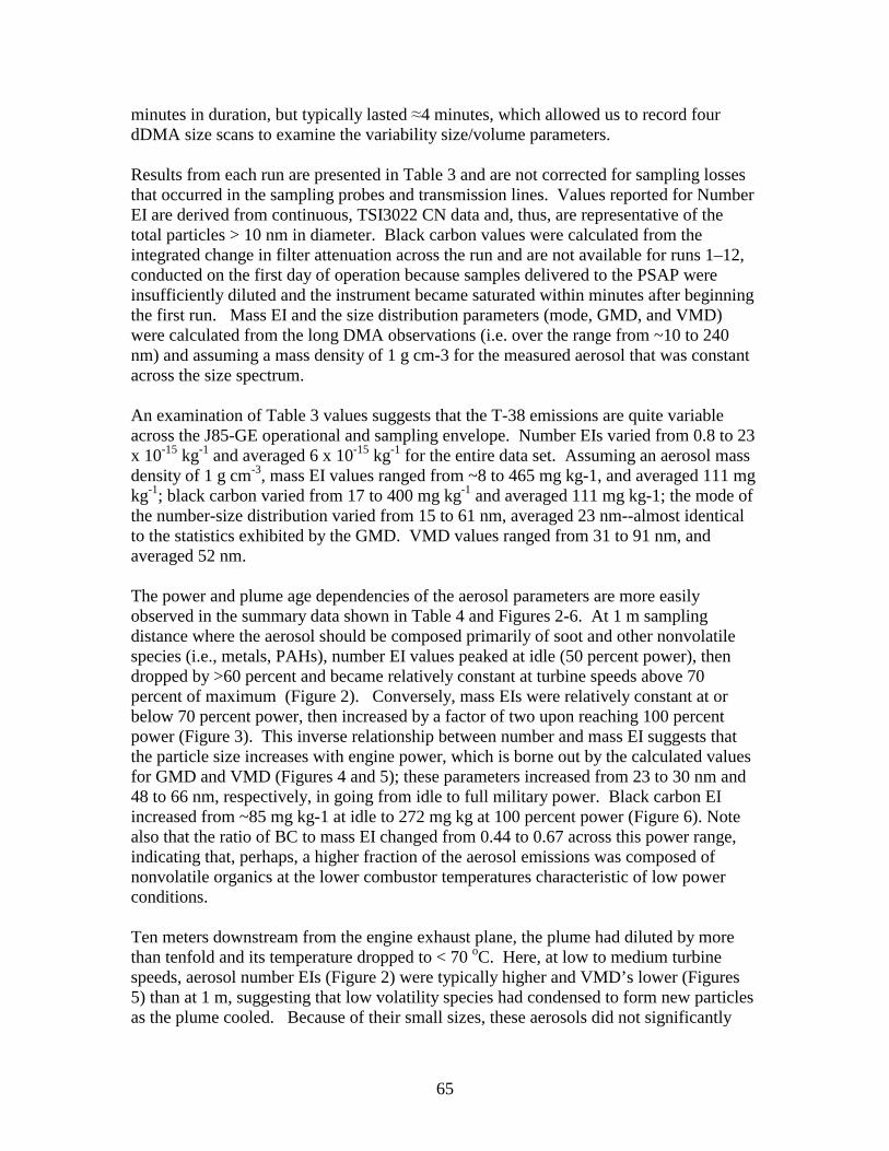
65

minutes in duration, but typically lasted ≈4 minutes, which allowed us to record four dDMA size scans to examine the variability size/volume parameters. Results from each run are presented in Table 3 and are not corrected for sampling losses that occurred in the sampling probes and transmission lines. Values reported for Number EI are derived from continuous, TSI3022 CN data and, thus, are representative of the total particles > 10 nm in diameter. Black carbon values were calculated from the integrated change in filter attenuation across the run and are not available for runs 1–12, conducted on the first day of operation because samples delivered to the PSAP were insufficiently diluted and the instrument became saturated within minutes after beginning the first run. Mass EI and the size distribution parameters (mode, GMD, and VMD) were calculated from the long DMA observations (i.e. over the range from ~10 to 240 nm) and assuming a mass density of 1 g cm-3 for the measured aerosol that was constant across the size spectrum. An examination of Table 3 values suggests that the T-38 emissions are quite variable across the J85-GE operational and sampling envelope. Number EIs varied from 0.8 to 23 x 10-15 kg-1 and averaged 6 x 10-15 kg-1 for the entire data set. Assuming an aerosol mass density of 1 g cm-3, mass EI values ranged from ~8 to 465 mg kg-1, and averaged 111 mg kg-1; black carbon varied from 17 to 400 mg kg-1 and averaged 111 mg kg-1; the mode of the number-size distribution varied from 15 to 61 nm, averaged 23 nm--almost identical to the statistics exhibited by the GMD. VMD values ranged from 31 to 91 nm, and averaged 52 nm. The power and plume age dependencies of the aerosol parameters are more easily observed in the summary data shown in Table 4 and Figures 2-6. At 1 m sampling distance where the aerosol should be composed primarily of soot and other nonvolatile species (i.e., metals, PAHs), number EI values peaked at idle (50 percent power), then dropped by >60 percent and became relatively constant at turbine speeds above 70 percent of maximum (Figure 2). Conversely, mass EIs were relatively constant at or below 70 percent power, then increased by a factor of two upon reaching 100 percent power (Figure 3). This inverse relationship between number and mass EI suggests that the particle size increases with engine power, which is borne out by the calculated values for GMD and VMD (Figures 4 and 5); these parameters increased from 23 to 30 nm and 48 to 66 nm, respectively, in going from idle to full military power. Black carbon EI increased from ~85 mg kg-1 at idle to 272 mg kg at 100 percent power (Figure 6). Note also that the ratio of BC to mass EI changed from 0.44 to 0.67 across this power range, indicating that, perhaps, a higher fraction of the aerosol emissions was composed of nonvolatile organics at the lower combustor temperatures characteristic of low power conditions. Ten meters downstream from the engine exhaust plane, the plume had diluted by more than tenfold and its temperature dropped to < 70 oC. Here, at low to medium turbine speeds, aerosol number EIs (Figure 2) were typically higher and VMD’s lower (Figures 5) than at 1 m, suggesting that low volatility species had condensed to form new particles as the plume cooled. Because of their small sizes, these aerosols did not significantly

66

add to the mass loading (Figure 3), except at the idle condition (50 percent) where the mass EI is twice the value observed at 1 m. This might be related to the longer growth period experienced by the aerosols in the low velocity plume, the propensity of the engine to emit more condensable hydrocarbons at low powers, or it might simply be caused by poor sampling statistics. Samples collected from the 25 m inlet exhibited even higher number EIs (Figure 2) but the trend in mass EIs could not be delineated because, at that sampling distance, concentrations were too variable across the 60 second scan time of the DMA to yield reliable size distributions. Black carbon EIs tended to increase with sampling distance (Figure 6), which may be caused by a number of factors. First, the freshly formed sulfate and organic aerosols could have deposited on the PSAP filter and caused enhanced scattering that is, from the instruments perspective, indistinguishable from the absorption due to soot. Ideally, simultaneous measurements of aerosol scattering coefficient (σs) at 565 nm would have been recorded and used to correct the measured absorption coefficient via the method developed by Bond et al., (1999). Lacking these measurements, we may in the future use the measured size distributions and Mie theory to calculate σs to evaluate the extent to which scattering effects the measurement. We note, however, that most of the newly formed sulfate particles are <<100 nm in diameter and should not exhibit appreciable scattering. On the other hand, organic molecules condensing upon existing soot particles could have increased their scattering cross-sections, but the size distribution scans, at least at 10 m, do not suggest that any great changes occur in the population of aerosols in the 50 to 250 nm size range. Another entirely different explanation is that aerosol losses were greater in the 1 m inlet than the 10-m inlet probe. It is easy to visualize enhanced losses at the 1 m sampling distance because the environment there is very hot (>300 oC) and highly turbulent (mean velocities of 50 to 400 m s-1) and aerosol concentrations are extremely high (~108 cm-3 ) which might lead to rapid losses though thermophoretic effects, Brownian diffusion, turbulent deposition, and coagulation. However, this does not account for why the 25 m values are in most cases higher than those observed at 10 m. Perhaps the primary factor is that, as the plume ages, the small soot particles grow through agglomeration, coagulation, or accretion of gas phase material to sizes that are less susceptible to loss in the inlet/sample transport systems. We note that even with the low transmission efficiency of the sampling probes for nucleation mode aerosols (<20 percent for diameters < 10 nm), size scans recorded by U. Minnesota at the 1-m sampling distance showed there were large numbers of nonvolatile aerosol in the 3 to 10 nm size range, which supports the notion that a significant fraction of the absorbing aerosols may have escaped detection at the closest sampling distance. Indeed, because jet engine exhaust plumes contain a great deal of nanometer-sized particles and condensable material (i.e., water, sulfuric acid, organics), we have observed that aerosol characteristics are highly dependent upon the details of sample collection and dilution. For example, experiments conducted at Langley in the summer of 1999 indicated that the T-38A number EI at any given power could be manipulated by a factor of eight by turning on and off the cooling water supplied to the sample collection probe that was positioned 1-m downstream of the exhaust plane (Cofer et al., 2001). To

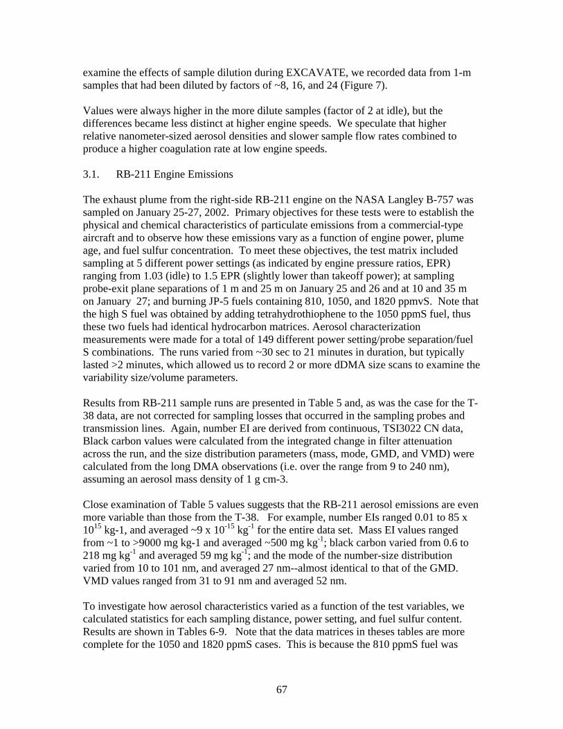
67

examine the effects of sample dilution during EXCAVATE, we recorded data from 1-m samples that had been diluted by factors of ~8, 16, and 24 (Figure 7). Values were always higher in the more dilute samples (factor of 2 at idle), but the differences became less distinct at higher engine speeds. We speculate that higher relative nanometer-sized aerosol densities and slower sample flow rates combined to produce a higher coagulation rate at low engine speeds. 3.1. RB-211 Engine Emissions The exhaust plume from the right-side RB-211 engine on the NASA Langley B-757 was sampled on January 25-27, 2002. Primary objectives for these tests were to establish the physical and chemical characteristics of particulate emissions from a commercial-type aircraft and to observe how these emissions vary as a function of engine power, plume age, and fuel sulfur concentration. To meet these objectives, the test matrix included sampling at 5 different power settings (as indicated by engine pressure ratios, EPR) ranging from 1.03 (idle) to 1.5 EPR (slightly lower than takeoff power); at sampling probe-exit plane separations of 1 m and 25 m on January 25 and 26 and at 10 and 35 m on January 27; and burning JP-5 fuels containing 810, 1050, and 1820 ppmvS. Note that the high S fuel was obtained by adding tetrahydrothiophene to the 1050 ppmS fuel, thus these two fuels had identical hydrocarbon matrices. Aerosol characterization measurements were made for a total of 149 different power setting/probe separation/fuel S combinations. The runs varied from ~30 sec to 21 minutes in duration, but typically lasted >2 minutes, which allowed us to record 2 or more dDMA size scans to examine the variability size/volume parameters. Results from RB-211 sample runs are presented in Table 5 and, as was the case for the T-38 data, are not corrected for sampling losses that occurred in the sampling probes and transmission lines. Again, number EI are derived from continuous, TSI3022 CN data, Black carbon values were calculated from the integrated change in filter attenuation across the run, and the size distribution parameters (mass, mode, GMD, and VMD) were calculated from the long DMA observations (i.e. over the range from 9 to 240 nm), assuming an aerosol mass density of 1 g cm-3. Close examination of Table 5 values suggests that the RB-211 aerosol emissions are even more variable than those from the T-38. For example, number EIs ranged 0.01 to 85 x 1015 kg-1, and averaged ~9 x 10-15 kg-1 for the entire data set. Mass EI values ranged from ~1 to >9000 mg kg-1 and averaged ~500 mg kg-1; black carbon varied from 0.6 to 218 mg kg-1 and averaged 59 mg kg-1; and the mode of the number-size distribution varied from 10 to 101 nm, and averaged 27 nm--almost identical to that of the GMD. VMD values ranged from 31 to 91 nm and averaged 52 nm. To investigate how aerosol characteristics varied as a function of the test variables, we calculated statistics for each sampling distance, power setting, and fuel sulfur content. Results are shown in Tables 6-9. Note that the data matrices in theses tables are more complete for the 1050 and 1820 ppmS cases. This is because the 810 ppmS fuel was

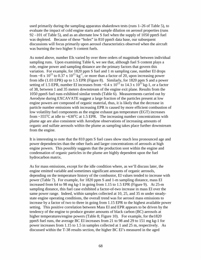
68

used primarily during the sampling apparatus shakedown tests (runs 1–26 of Table 5), to evaluate the impact of cold engine starts and sample dilution on aerosol properties (runs 92 –101 of Table 5), and as an alternate low S fuel when the supply of 1050 ppmS fuel was depleted. Because of these “holes” in 810 ppmS data base, our subsequent discussions will focus primarily upon aerosol characteristics observed when the aircraft was burning the two higher S content fuels. As noted above, number EIs varied by over three orders of magnitude between individual sampling runs. Upon examining Table 6, we see that, although fuel S content plays a role, engine power and sampling distance are the primary factors that govern this variation. For example, for 1820 ppm S fuel and 1 m sampling case, number EI drops from ~8 x 1015 to 0.37 x 1015 kg-1, or more than a factor of 20, upon increasing power from idle (1.03 EPR) up to 1.5 EPR (Figure 8). Similarly, for 1820 ppm S and a power setting of 1.5 EPR, number EI increases from ~0.4 x 1015 to 14.3 x 1015 kg-1, or a factor of 38, between 1 and 35 meters downstream of the engine exit plane. Results from the 1050 ppmS fuel runs exhibited similar trends (Table 6). Measurements carried out by Aerodyne during EXCAVATE suggest a large fraction of the particles present at low engine powers are composed of organic material, thus, it is likely that the decrease in particle number emissions with increasing EPR is caused by more efficient combustion of low volatility fuel components as the engine exhaust gas temperature (EGT) increases from ~355oC at idle to ~630oC at 1.5 EPR. The increasing number concentrations with plume age are also consistent with Aerodyne observations of increasing amounts of organic and sulfate aerosols within the plume as sampling takes place further downstream from the engine. It is interesting to note that the 810 ppm S fuel cases show much less pronounced age and power dependencies than the other fuels and larger concentrations of aerosols at high engine powers. This possibly suggests that the production soot within the engine and condensation of organic particles in the plume are highly dependent upon the fuel hydrocarbon matrix. As for mass emissions, except for the idle condition where, as we’ll discuss later, the engine emitted variable and sometimes significant amounts of organic aerosols, depending on the temperature history of the combustor, EI values tended to increase with power (Table 7). For example, for 1820 ppm S and 1-m sampling distance, mass EI increased from 64 to 98 mg kg-1 in going from 1.15 to 1.5 EPR (Figure 9). At 25-m sampling distance, this fuel case exhibited a factor-of-two increase in mass EI over the same power range. Indeed, within samples collected at 10, 25, and 35 m under steady-state engine operating conditions, the overall trend was for aerosol mass emissions to increase by a factor of two to three in going from 1.15 EPR to the highest available power setting. This positive correlation between Mass EI and EPR appears to be driven by the tendency of the engine to produce greater amounts of black carbon (BC) aerosols at higher temperatures/engine powers (Table 8; Figure 10). For example, for the1820 ppmS fuel runs, the average BC EI increases from 21 to 98 and 29 to 151 mg kg-1 for power increases from 1.15 to 1.5 in samples collected at 1 and 25 m, respectively. As discussed within the T-38 results section, the higher BC EI’s measured in the aged

69

plumes may be related to lower aerosol losses in the secondary sampling probes or light-scattering from condensed organic or sulfate particles. In any case, from examining the 1 m data in Tables 7 and 8, we deduce that BC accounts for < 10 percent of total aerosol emissions at idle but almost 100 percent for the higher power settings. Examining the data in Table 7 and Figure 9, we also see that mass EIs increased with plume age, presumably due to condensation of low volatility material as the emissions cooled. For example, for 1820 ppmS fuel and an EPR of 1.4, mMass EI increased from 95 to 247 mg kg-1 between samples collected at 1 and 35 m. The 1050 ppmS fuel exhibited the same, factor of two-to-three trend, but age-related enhancements in the 810 ppmS cases were more modest and harder to discriminate because of poor sampling statistics and the fact that much of the low to medium power data was acquired during non-steady state conditions. The observed anti-correlation between the Number and Mass EIs suggests that particle size increased with engine power; this is supported by the GMD and VMD data shown in Table 8. For example, for 1820 ppmS and 1 m sampling, GMD increased from 20 to 38 nm and the VMD from 45 to 103 nm in going from 1.15 to 1.5 EPR (Figures 11 and 12). Similar trends are seen in the 1050 ppmS data, but again, the 810 ppmS size statistics appear somewhat random which is probably due to the data set for this fuel being heavily biased toward non-steady state sampling conditions. The GMD data also support the notion that new particles form within the plume as it cools and ages. Note that for 1820 ppmS fuel and 1.5 EPR, GMD decreases from 38 to 27 nm in going from 1 to 25 m downstream of the engine exhaust plane (Figure 11). The age-related changes in mean size were even more dramatic in measurements recorded by the University of Minnesota nanometer aerosol analyzer (nASA), which is sensitive to sizes down to 3 nm (the effective cutoff of the long DMA used to acquire Table 6-8 data was >8 nm); GMD values calculated from its size scans drop to < 12 nm for many of the 35 m samples (see Appendix C of this Report). Individual size distributions of the aged emissions are bimodal in nature and show that the decrease in GMD is caused by the nucleation and growth of aerosols at diameters less than 30 nm (Figure 13). Mass spectrometer measurements suggest these particles are composed of either sulfuric acid or neutralized sulfate. Their large concentrations tend to dominate number EI values; however, they contribute only a few percent to the overall mass loading and produce essentially little change in calculated VMDs (Figure 12). The fact that mass emissions increase by factors of two or more between the 1 and 35 m samples can be partially attributed to low volatility hydrocarbons condensing upon existing black carbon aerosols (Appendix D of the EXCAVATE Report). A primary EXCAVATE objective was to examine the role that fuel S played in the formation of secondary aerosols within the aircraft exhaust plume. Disregarding data acquired at low power settings (1.03 and 1.15 EPR) where transient emissions of unburned organic compounds biased the statistics, the data shown in Tables 7 and 8 indicate that downstream particle loadings were significantly greater for the 1820 ppmS than 1050 ppmS cases. For example, at 1.3 EPR and a 10 m sampling distance, number

70

and mass EI values were a factor 3 and ~14 percent greater, respectively, for 1820 ppmS fuel in comparison to the 1050 ppmS fuel. Size distributions recorded at 25 and 35 m indicate the primary difference between the two fuel cases is the relative amplitude of the nucleation mode peak that forms at diameters < 30 nm—it is clearly much larger in the higher fuel S samples. At 25 m sampling distance the greater contribution from nucleation mode aerosols to the number-based size distribution causes the GMD to be shifted to slightly smaller diameters for the 1820 ppmS relative to the 1050 ppmS emissions (Table 8). In contrast, at 35 m GMDs are actually smaller for the lower fuel S cases. Note that between 25 and 35 m and for engine powers of 1.3 and 1.4 EPR, Number EIs increased by factors 3 to 4 in the low S plume, but by < 2 for the high S emissions (Table 7). Also the differences in number EIs between the two fuels are much less at 35 m than at 25 m (20 to 40 percent as opposed to factors of 2 to 3). Thus, it appears that particle formation and growth processes, though highly active in both cases, occur at slower rates in the lower S fuel cases because of the lower saturation ratio of sulfuric acid within the exhaust plume. Using BC and aerosol mass EI values for the various sampling distance/fuel S combinations, it is possible to estimate the relative contributions of organic and sulfate aerosols to overall aerosol mass loadings. For a power setting of 1.3 EPR, the residual Mass EI (i.e., the difference between total aerosol and BC EI) varies from -20 to 94 mg, and -11 to 138 mg kg-1, for the 1050 and 1820 ppmv, respectively, between the 1 and 35 m sampling distance (Figure 14). Assuming that organic aerosol loadings are identical in the two fuel cases, we calculate that the extra 770 ppmS in the high S fuel enhanced the overall aerosol Mass EI ~44 mg kg-1 in the 35 m samples. Using an average sulfate aerosol molecular weight of 150 g mole-1 to make allowances for hydration and partial neutralization of sulfuric acid by ambient ammonia or sea salt, the 44 mg kg-1 EI corresponds to a fuel S conversion factor, ε, of ~1.2 percent which is consistent with many previous observations (Schumann et al., 2002). A similar analysis of data recorded at 1.4 EPR yields ε ~0.5 percent at the 35 m sampling distance; this lower value is probably related to the shorter growth period experienced by aerosols in the higher velocity 1.4 EPR plume. Amazingly, if we use the inferred sulfate conversion efficiencies shown in Figure 14 to back-calculate organic aerosol Eis, we obtain exactly the same values at all sampling distances for the two fuels, although the values are negative for the 1 and 10 m cases which indicates that either the aerosols mass density is > 1 g cm-3 or that the absorption cross-section for soot is >7 m2 g-1. If we subtract the 1 m organic aerosol EI from the 35 m value, we find that ~70 mg kg-1 of secondary organic particulate matter formed as the 1.3 EPR plume cooled and expanded. This observation is consistent with the simultaneous composition measurements that showed the engine emitted significantly greater quantities of condensed hydrocarbons than of sulfate under steady state conditions (see Aerodyne AMS report). Plots of inferred sulfate and organic aerosol EI vs distance (Figure 14) also provide information on the relative rates that the two volatile species condense. Note that sulfate aerosol mass increases rapidly between 1 and 10 meters then begins to level off whereas organic aerosol EI continues to increase as the plume ages, which indicates that sulfuric acid is less volatile than many of the organic species that are condensing within the

71

plume. The steep slope of the curve between 25 and 35 m suggests that significant additional organic aerosol would be formed as the plume undergoes further aging. As noted above, data acquired at idle and 1.15 EPR were highly variable and depended more on how long the engine had been running, the time since power change, and the details of sample collection than upon the selected test variables of fuel S or plume age. For example, Figure 15 shows a 1-second resolution time-series plot of the RB-211 number EI for 1820 ppmS fuel and samples extracted at 1 and 25 m downstream of the engine exhaust plane. The engine had cooled for ~1 hr prior to the beginning of the record. Note that 1 m values are ~1016 kg-1 at startup then drift downward by a factor of 5 over the 20 minute run at 1.03 EPR. When power is increased to 1.15 EPR, number EI jumps back up to 10-16 kg-1, then begins to drift downward as the engine re-equilibrates to the new fuel flow rates and combustor temperatures, reaching ~1015 kg-1 just before the power is increased to 1.3 EPR Similar jumps in number EI occurred after each power change, although the subsequent drift was less at the higher EPR settings. Note that number EI values also took a few minutes to settle down after flow was switched from the 25 m to the 1 m inlet probe (Figure 15). When sample air was drawn from the downstream probe, flow was completely stopped in the 1 m inlet lines trapping a significant volume of air that would, because of diffusion and deposition losses, within a few minutes become essentially particle-free. Thus, we speculate that the initial drop in aerosol number density observed when sampling from the 1 m inlet resumed was caused by dilution with aerosol-depleted air. Changes in temperature may also contribute by causing differential thermophoretic losses as the probe reheated to reach thermal equilibrium with the impinging sample flow. Transients in the RB-211 aerosol number density emissions were accompanied by equally dramatic changes in mass emissions. Figure 16 displays a 1-minute resolution time-series of mass EI corresponding to the number EI data shown in Figure 15. At engine start, mass EI peaked at ~3000 mg kg-1, then decreased to < 100 mg kg-1 some 10 minutes later. Although a reduction contributed to this change, it was primarily driven by a shift in the number modal diameter from ~100 nm to < 25 nm during this time period (Figure 17 and 18). The power increase from 1.03 to 1.15 EPR produced similar enhancements in mass emissions (and GMD) that required 3 to 4 minutes to settle back down to a steady state value(s). Order-of-magnitude transients also occurred when power was reduced from 1.5 EPR to idle. These observations are consistent with aerosol measurements made by other groups during EXCAVATE [see Appendices B, C, and D] and were found to occur for all fuel types and sampling conditions. To our knowledge, there are no published reports of transient aerosol or gas phase emissions from jet turbines, but it is a well-know phenomena in diesel engines (refs). In terms of an explanation, simultaneous aerosol mass spectral data indicate the transient aerosols were composed of organic species that possessed mass signatures similar to those of engine oil. After cold starts and power changes, it takes a few minutes for the compressor stages to reach thermal equilibrium and establish the very tight component tolerances necessary for optimum engine performance. We speculate that during this thermal adjustment period, a minor amount of engine oil leaks around the seals and produces the observed organic

72

aerosol enhancements. It is significant to note that the enhancements were present in samples collected at 1 m where the exhaust gas temperature was quite high; this supports the idea that they were composed of relatively nonvolatile species such as those present in thermally stable turbine engine lubricating fluid. It is also possible that a fraction of these particles were derived from unburned fuel, as whole air samples, collected within the plume shortly after engine start, contained significant enhancements in relatively low-molecular weight hydrocarbon species (see Appendix E). Unburned fuel is certainly present within the exhaust just before combustor ignition and may take a few minutes to volatilize and be cleared from the downstream sections of the engine. 4.0. Conclusions Extensive characterization measurements were made of aerosols collected at various points downstream from the engine exhaust planes of the Langley T-38A and B-757 aircraft. Results indicate these aircraft emit significant quantities of black carbon and that volatile species condense and grow very rapidly within their exhaust plumes as the emissions cool and age. For the J85-GE engine, aerosol properties in samples collected at 1 m depended upon dilution ratio, particularly for low power settings where high levels of volatile organic species were present. Maintaining constant dilution ratios of 8:1 to minimize coagulation effects, number EIs measured at 1 m sampling distance peaked at idle, decreased monotonically with increasing engine power, and averaged ~3 x 1015 kg-1 at typical cruise power settings (70-80 percent of maximum RPM) which is comparable to nonvolatile aerosol EI values observed behind the aircraft in flight (Anderson et al., 1999). Mean particle volume diameters increased with combustor temperature ranging from ~48 nm at idle to 66 at takeoff power (100 percent). This produced mass EIs that varied from ~190 to 380 mg kg-1 at the extremes of the power range and averaged ~200 mg kg at cruise settings. Black carbon apparently comprised the greatest fraction of the emissions, contributing ~50 percent at idle and 67 percent at takeoff power. Samples collected 10 and 25 m behind the engine exhibited significantly greater number EIs and slightly increased black carbon EIs. The enhancement in relative aerosol number concentrations is attributed to condensation of sulfate and low volatility organic species. Interestingly, the added material caused the VMD of size distributions observed at 10 m to shift to smaller diameters but produced no noticeable change in GMD, suggesting that the aerosols were simply being added to an already existing, dominant mode. Size distributions recorded 25 m downstream were too variable to provide data to further elucidate this problem. As for the age-dependence in black carbon EI, several factors may have contributed including the uncorrected effects of sulfate aerosol scattering, more efficient sample collection by the downstream probes, and growth of the soot particles to sizes less susceptible to diffusional losses. The RB211 engine shared the J85-GE’s tendency to produce fewer particles of larger size and greater black carbon content with increasing power, but it also displayed a propensity to emit huge quantities of organic aerosols after cold starts or following power changes, particularly within its low power operating range. For steady-state operating conditions

73

and 1 m sampling, the engine nominally produced between 0.5 and 5 x 1015 kg-1 across the power range from 1.03 to 1.5 EPR (note that 1.7 EPR is takeoff power) with values of ~1015 kg-1 typical for cruise power settings of 1.3 to 1.4 EPR. Excluding transient data, GMD and VMD values varied from 20 to 35 and 45 to 100 nm, respectively, between the power extremes and were typically 25 and 85 nm, respectively, for cruise. Stable mass EIs were difficult to delineate for idle conditions because of transient effects, but median values varied from ~50 to 100 mg kg-1 between 1.15 and 1.5 EPR and were typically in the range of 60 to 80 mg kg-1 for cruise power settings. For the 1 m sampling and assuming an aerosol mass density of 1 g cm-3, black carbon accounted for essentially 100 percent of the observed aerosol emissions over the medium to high power operating range. Levels of volatile particulates within the exhaust plume increased dramatically as it aged. Number EIs depended upon fuel S content and were, for the higher engine powers, factors of 10 to 40 greater at 25 to 35 m downstream in comparison to the 1 m measurements. Corresponding Mass EI enhancements were more moderate but still quite evident. Based partly on simultaneous composition measurements acquired by Aerodyne, we speculate that the increase in aerosol number EI was driven primarily by formation of new sulfate aerosols in the size range below 30 nm, and that increased mass concentrations were caused not only by the condensation of the sulfates but accretion of low volatility organic compounds onto existing soot particles. Contrasting the data acquired using fuels of different sulfur content at a single power settting, we calculated that the 770 ppm higher S content in the 1820 ppmS fuel was responsible for producing >40 mg kg-1 of the aerosol mass sampled at 35 m; this corresponds to a fuel S conversion efficiency of 1.2 percent which is comparable to previous observations. Our calculations also showed that organic aerosols contributed at least 70 mg kg-1 to the overall mass EI in samples collected at 35 m and that, given the steep increase in organic aerosol loading between the 25 and 35 m sampling distances, volatile organics would most likely continue to condense within the plume as it underwent additional cooling and aging. Aerosol mass emissions from the RB-211 after cold starts and power changes were significantly greater than observed when the engine was operating at thermal equilibrium. Indeed mass EIs approaching 10 g kg-1 were common as the engine idled just after combustor ignition and values exceeding 1 g kg-1 were frequently observed after power was increased from 1.03 to 1.15 EPR or when the engine was rapidly brought back to idle from medium to high power settings. These findings are likely to have significant implications for aircraft operations in terminal areas as every aircraft flown must at some point, undergo a cold start and experience a sometimes large number of brief power surges during taxi to and from passenger loading gates. Current emission models that employ steady-state emission factors are thus likely to severely underestimate actual aerosol concentrations within the aircraft operating areas. Data and analyses presented within this report will do little to resolve the debate over what aerosol parameters should be measured and what sampling distances should be employed to replace/augment the smoke number standards currently required for

74

emission qualification for jet turbine engines. The SAE-31 committee has suggested DMA-determined number EIs, GMDs and geometric standard deviations (GSD) of the size distributions as measured in samples extracted from 1 m downstream of the engine exit plane as possible candidates. This study has shown that, even at the close sampling range, number EIs and GMDs are highly variable depending upon fuel composition, power setting, sample dilution, power-change history. We elected not to discuss GSD values because measured size distributions were often multimodal and seldom exhibited simple log-normal characteristics. In addition, samples collected at 1 m fail to provide any information about the more volatile aerosols that condense slightly further downstream and are likely to have equally significant impacts upon local air quality. 5.0. References Anderson, B. E., et al., 1998: Airborne observations of aircraft aerosol emissions I: Total

nonvolatile particle emission indices, Geophys. Res. Let., 25, pp. 1689-1692. Bond, T. et al., 1999: Calibration and intercomparisons of filter-based measurements of

visible light absorption by aerosols, Aero. Sci. Tech., 30, pp. 582-600. Cofer, W. R., et al., 1997: Calibration and demonstration of a condensation nuclei

counting system for airborne measurements of aircraft exhausted particles, Atmospheric Environment, 32, pp. 169-176.

Cofer, R., et al., 2001: Results of the August 1999 Aerosol Measurement Intercomparison Workshop, T-38 aircraft sampling phase, NASA/TM-2001-211226.

Petzold, A., and A. Dopelheuer, 1998: Re-examination of black carbon mass emissions indices of a jet engine, Aero. Sci. Tech., 29, pp. 355-356.

Shumann, U., et al., 2002: Influence of fuel sulfur on the composition of aircraft exhaust plumes: The experiments SULFUR 1-7, J. Geophys. Res., 107, 10.1029/2001JD000813.

Wang, S. and R. Flagan, 1990: Scanning Electrical Mobility Spectrometer, Aero. Sci. Tech., 13, pp. 230-240.

75

nuR hca

E fo noitaruD eht roF detalucla

C sci tsitatS el citraP ;A83-

T yelgnaL dn ihe

B snuR elp

maS  .3 elb aT

DMV

DMG

ed oM

) gk/ gm( I

E  s saM) gk/g

m(  no bra c kcalB  

)g k/#(  IE re b

muN     

ec natsiD

eni gnE

d nE

tratSn ailuJ

tseT

)mn(

)mn(

)m n(

dtSgv

Av ed  dt S

g vA

ved  dtSgv

A)

m()RP

E( rewo p

s ces TU

sces TU

etadnur

8432

4 232

3 91 

 41 +

E 19.251+

E 62 .31

0500137

0662722

11 5

3 21 2

6671

  

4 1+E08.1

5 1+E39 .2

106

33737051 37

222

554 2

2 22 2

49 1 

 41+

E3 5. 151 +

E 97 .21

0 705347

087 3722

395

6 24 2

8 441 2

  

41+E5 1. 1

51 +E 12 .2

108

07947074 47

224

1672

6235 1

722 

 3 1+

E 68.45 1+

E96 .11

0909557

0025722

566

2 39 2

1 5168 3

  

31 +E3 6. 2

51+E8 7. 1

1001

0426725757

226

2532

1 24

01 1 

 31 +

E0 4. 651+

E1 1. 21

0734567

0936722

71 5

4222

78 51

  

31+E 59.5

5 1+E 47 .2

105

03867596 67

228

0542

4233 2

1 81 

 41+

E 17.15 1+

E 78 .21

0506977

004 7722

976

3 30 3

35178 3

  

31+E0 9. 2

51 +E9 7. 1

1001

0158 706087

2201

9572

6291

341 

 31+

E 67.95 1+

E 14.21

0777787

0968722

1125

4232

348 71

  

41+E 74 .1

5 1+E 80.3

105

4309700887

2221

745 2

7 27 4

27 121

1 941 +

E5 3. 751+

E3 7.51

0551435

0613542

3164

3222

37 1673

2 438

51+E 21 .3

61+E90.1

0105

0083 564435

4241

6432

2257

4222 4

4951+

E 43 .361+

E15.101

060814 5

0883542

5194

129 1

6501

207

4 1+E61.1

51+E29.3

106

0774508345

4261

2522

0 27

6113

684 1+

E63.151+

E48.31

0759055

0084542

7134

1212

151 91

937 9

51 +E 0 4.4

61+E1 4. 1

0 107

01 75502 155

428 1

6 42 2

126 7

96 11 2

065 1+

E23.351+

E 08 .60 1

0 80 1165

0 385542

915 5

3 21 2

3 720 1

476

3 1+E20.8

51+E 68 .2

10 8

5 26650 9165

4202

9572

4276 1

3 022

8113 1+

E 15.751 +

E 21.31

0 90 396 5

0 876542

122 5

6 272

02251

827

4 1+E 06 .5

51 +E35.4

0109

0457 55 507 5

4222

8 59 2

9289

4428

0 314 1+

E 88 .651 +

E12.401

0010397 5

0 857 542

3206

726 2

9016 42

48 91

41+E 80.3

51+E90.4

1001

5748 50308 5

4242

4622

9134

0 67

5531+

E88.751+

E44.21

0707785

2758542

528 5

1281

2 0 1601

3 215

41+E66.7

51+E02.4

0107

0739504885

4262

055 2

5 20 3

6471

634 1+

E 22.751+

E8 0.201

050469 5

0449542

724 5

1 202

1 504

313

3 1+E 06.1

51+E5 8.1

105

0699 505795

4282

1462

7253

4 92 

 4 1+

E 66 .661+

E5 0. 11

055923 5

0003592

9 29 3

6 27 2

1 436 64

7367

51+E 62.2

61+E3 7. 1

105

06 53507 335

920 3

5 39 1

8 10 01

3 126

5751+

E 11.761+

E1 3. 21

0506 935

00 73592

1 329

8516

8257

913 21

41+E72.1

51+E 92 .4

105

00 95502 755

9223

  

  

 71

3215 1+

E63.161+

E 60 .10 1

0 50 8165

5 606592

33

76

dedulcnoC  . 3 elba

T

DMV

DMG

e doM

) gk /gm ( I

E  ssaM

) g k/gm(  nobr a c  kc al

B )gk/ #( I

E r ebmu

N    ec natsi

De nig n

Edn

Etr atS

n ailuJtse

T)

m n()

m n()

mn(dtS

g vA

ved dtSgv

Ave d  dtS

g vA

)m(

)RP

E( rewo p

sc es TU

sces TU

etadnur

  

  

 01

41 141+

E 22 .551 +

E7 9. 81

0508365

0536592

4394

3291

61001

298

41+E 43 .1

51 +E8 4. 4

106

0076504565

9253

8 412

814 1

01 15

5 641 +

E0 1. 351+

E 38 .51

0 651965

0276592

6384

1281

71 114 1

019 1

41 +E9 6. 4

51+E 37 .5

10 6

0317503965

9273

541 2

8 1 

02143

34151+

E 70 .26 1+

E50. 101

0606375

2817592

83 

  

  

137 7

5 1+E15 .1

41+E 43 .8

5 206

0847529375

9293

3991

51 

87

9 13 1+

E48 .751 +

E 33 .31

0606575

0157592

041 5

3 21 2

287

309

31 +E 6 8.5

5 1+E94 .3

107

5977505675

9214

1532

9106

896

4 63 1+

E51 .751 +

E0 9. 31

0759975

0387592

2415

2281

 5 9

618 3

4 1+E23 .1

51 +E5 3. 4

107

6128542085

9234

740 2

8 14

983 5

9 5141+

E2 8. 85 1+

E 21 .901

0705485

0428592

4434

2232

 841

0281 1

5 1+E 01 .1

61+E31.1

5207

0278508485

9254

1412

12 

186

494 1+

E51 .451+

E08.81

0754885

5378592

642 5

4 212

 0 7

457

31 +E4 7. 7

51+E35.2

108

0809503985

9274

9 422

12 

8 58

3531 +

E1 7. 751 +

E4 0.31

0 80 339 5

06 1959 2

8 415

3212

3185

871

31+E9 6.6

51 +E8 8.2

10 8

0459 509395

929 4

8 41 2

6 1 

8 567

8 615 1+

E0 0.151+

E66.801

0857795

5559592

0 534

1281

 62 1

330 41

41+E6 8.6

61+E01.1

5208

5699509795

921 5

657 2

4 2 

7 717 1

40131+

E32.751+

E39.21

0968106

5400692

2515

4212

 9 9

99 9

41+E59.1

51+E45.3

109

0040604206

9235

0532

12 

50 191

6741+

E75.151+

E39.31

0902606

0340692

4515

328 1

 29

7 54 71

41 +E4 3.4

51+E91. 5

0109

56 8060 76 06

9255

7 42 2

8 1 

5 310 5

3 7141 +

E4 2.451+

E25. 952

0906 016

588 0692

65 

  

  

70 9

31+E3 5.3

5 1+E74. 2

109

16 1164 2 116

9 275

9 59 2

9 2 

8 227

70331+

E99.451+

E 87 .31

00 15 4316

0 0 2169 2

859 5

8 29 2

5 40 82

9572

  

100 1

0 951 60 0 416

9 295

958 2

5 211

3 2261

07 2 

 1

00 10481 6

0 0 6169 2

0675

6252

 352

35004

41+E82.7

51+E75.6

01001

5012603916

9216

0682

5276 3

49 27 3

17341 +

E5 1.251 +

E30.652

0010332 6

0312692

2 625

321 2

2600 1

82 8

41 +E7 8.4

51+E7 7.6

10 7

5162609326

923 6

8402

8144

5745

1 851 +

E9 2.351+

E7 5.552

0 600926

0662692

4 62 3

0 21 2

 62

8146

51+E62.1

51+E79.6

0106

0692641926

9256

1512

8162

9653

6751+

E06 .151+

E95.601

0500 336

069 2692

66

77

snuR 

A83-T 

morF scitsitatS losoreA  .4 elba

T

)g k/gm(  I

E  CB

)mn(  

DMV

)m n(  

DMG

) gk/gm( I

E  ssaM

) gk/#(  IE re b

m uN

eborPe cnatsid

)m(

enignE

% r ewop

r ebmu

Nsnacs

amg iS

d eM

gvA

am gi S

deM

g vA

am g iS

deM

gvA

amg iS

deM

gvA

amg iS

deM

gvA

334 8

585

8 484

242

3255

87 1391

5 1+E4 .6

5 1+E0.4

51+E3.7

405

12 3

562 5

615

1 52

321 2

7 311 41

67 151+

E 1. 151+

E 1.451+

E2.46

06 

122 8

3753

5 555

23 2

22521

6514 91

5 1+E0.2

5 1+E6.3

51+E9.3

0107

 62

063 5

59 5

952

2242

55701

4 124 1+

E7.251+

E7.251+

E6.24

08 

5199

8991

161 6

31 2

528 7

0 2172 2

41 +E1. 7

51+E0.3

51+E8 .2

509

 64

272262

966

665

3 203

54 154 1

6835 1+

E5.151+

E0.251+

E4.26

001 

6 397

9 77

6464

332

3 225

3616 73

5 1+E9.3

51+E2.8

5 1+E1.7

405

0104

4 90 01

964

644

3 232

80 150 1

42251+

E8.361+

E0.161+

E0 .13

06 

457 9

2015

343 4

212

1 282

291 91

51+E7.4

51+E7.8

51+E6.8

307

 7 7

41 1411

164

6 41

222 2

5569

9 6151+

E2.151+

E3.751+

E3.72

08 

37321

32 10

2525

062

620

85251

41+E7.4

51+E6.4

51+E6.4

109

 19 1

5 6256 2

88 5

856

9292

0 213 41

44251+

E6.151+

E1.551+

E1.52

001 

397

9 74

454 5

432

3 20 31

1 61161

51+E8.4

51+E1.7

51+E1.7

206

52

8 1181 1

00 6

060

8282

0492

492 

61+E4.1

61+E4.1

107

 

0 4104 1

02 5

250

3232

0001

001 

61+E3.1

61+E3 .1

108

 

37 1371

084

8 40

020 2

05 7

57 

61 +E1. 1

61 +E1 .1

10 9

 

1 7317 3

02 3

230

0202

06 2

6 2 

51 +E0. 7

51 +E0.7

10 01

 

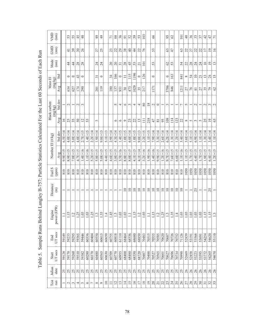
78

nuR hca

E fo sdnoce S 06 tsaL eht roF detaluc la

C scitsitatS elc itraP ;757-B yelgna

L dn iheB snu

R elpmaS   .5 elba

T

)gk/ #( IE r eb

muN

no b rac  kc alB

)g k/gm(

IE  s sa

M)g k/ g

m(tse

Tnur

nailuJetad

tratSsces 

TU

dnE

sces TU

enignE

)RP

E(  rew op

e cna tsiD

)m(

S leuF)

mpp(dtS

g vA

ve d  dtSg v

Av ed  dt S

g vA

edoM

)m n(

DMG

)m n(

DMV

)mn(

  

  

 1

6141+

E5.651 +

E9 .90 18

11. 1

9419582195

521

3 514

440

43 62

3 24 1+

E0.45 1+

E 9. 801 8

15 1. 1

3329507195

522

5 593

4 40

7261

534 1+

E 0. 551+

E 0. 7018

12.1

5929506295

523

540 3

8 23 4

4 712

0541 +

E0. 451 +

E7.40 18

152.1

5639501395

524

0 462

820

0923

2 15 1+

E7.261+

E 4. 1018

130.1

6449528395

525

  

  

  

3 55 1+

E4.161+

E 1. 1018

130.1

6330608206

526

  

  

  

 41+

E2.25 1+

E2 .50 18

152.1

4040607306

527

9 472

4213

102 

34 1+

E9.15 1+

E8.501 8

13.1

0550608406

528

9 45 2

4 20

911 

 3 1+

E 8. 951+

E 0. 5018

153.1

3160656506

529

  

  

  

 3 1+

E1 .551+

E 4. 4018

14.1

0560603606

5201

1 732

0243

08 1 

 4 1+

E9 .25 1+

E6.401 8

154.1

5570690706

5211

8 622

0266 1

73 15

641+

E3 .45 1+

E8 .3018

15.1

8180607706

5221

639 2

1 30

1394

65 1+

E4 .16 1+

E 5. 3018

130.1

0111655906

5231

198 3

8 21 1

0 36

951+

E 0. 151+

E 8. 8018

0130.1

4648600486

5241

2504

545 11

37 43

3241 +

E0.65 1+

E0.8018

011.1

6358608486

5251

9544

3569 11

92 0 14

2251 +

E0 .151 +

E 1. 401 8

0151 .1

0 868605 586

5261

3 522

120

5 34

3131+

E 0. 941 +

E1.4018

012.1

0588602786

5271

3 0167

1016 21

71 20 8

1 115 1+

E2 .261+

E2.3018

0130.1

3840770407

5281

  

  

 8 1

8 125 1+

E1.161+

E9.1018

011.1

5150788407

5291

663 5

3 50

17 112

7441+

E9.761+

E4.1018

0151.1

5550772507

5202

  

  

 0

1 841 +

E3.351 +

E9.9018

0 12.1

5850 75 6507

521 2

  

  

 1

5 941 +

E6.261 +

E2.1018

0152.1

0260 71 0607

522 2

5936

260

60733

90141+

E2.651+

E7.9018

013.1

7860772607

5232

2 674

3536 1

6481

41141+

E3.151+

E6 .70 18

0 15 3. 1

62 7 07696 07

5 242

  

  

 1

32141+

E2.151+

E6 .60 18

0 14. 1

25 7 07437 07

5 252

1 013 6

4 51 48

11 217

2241+

E4.361+

E 1.10 1 8

0130. 1

62 1 17099 07

5262

042 2

2 28

725

841+

E6.351+

E1.10 50 1

130. 1

93 825966 25

6272

637 2

8 245

6 71

531+

E1 .551 +

E 7. 105 01

130 .1

1 913585 825

6282

3 322

4201

182

341 +

E9 .651 +

E4. 405 01

5230.1

6 653532 235

6292

7322

4212

721

54 1+

E1 .151 +

E7. 105 01

130.1

1 963559 535

6203

2 471

6131

532

524 1+

E3.151+

E9.10501

151.1

4524527735

6213

7 491

9142

973

9141+

E4.351+

E4.60501

5251.1

0264556245

6223

1 761

3151

262

3641+

E1.151+

E2.10501

13.1

0115507645

6233

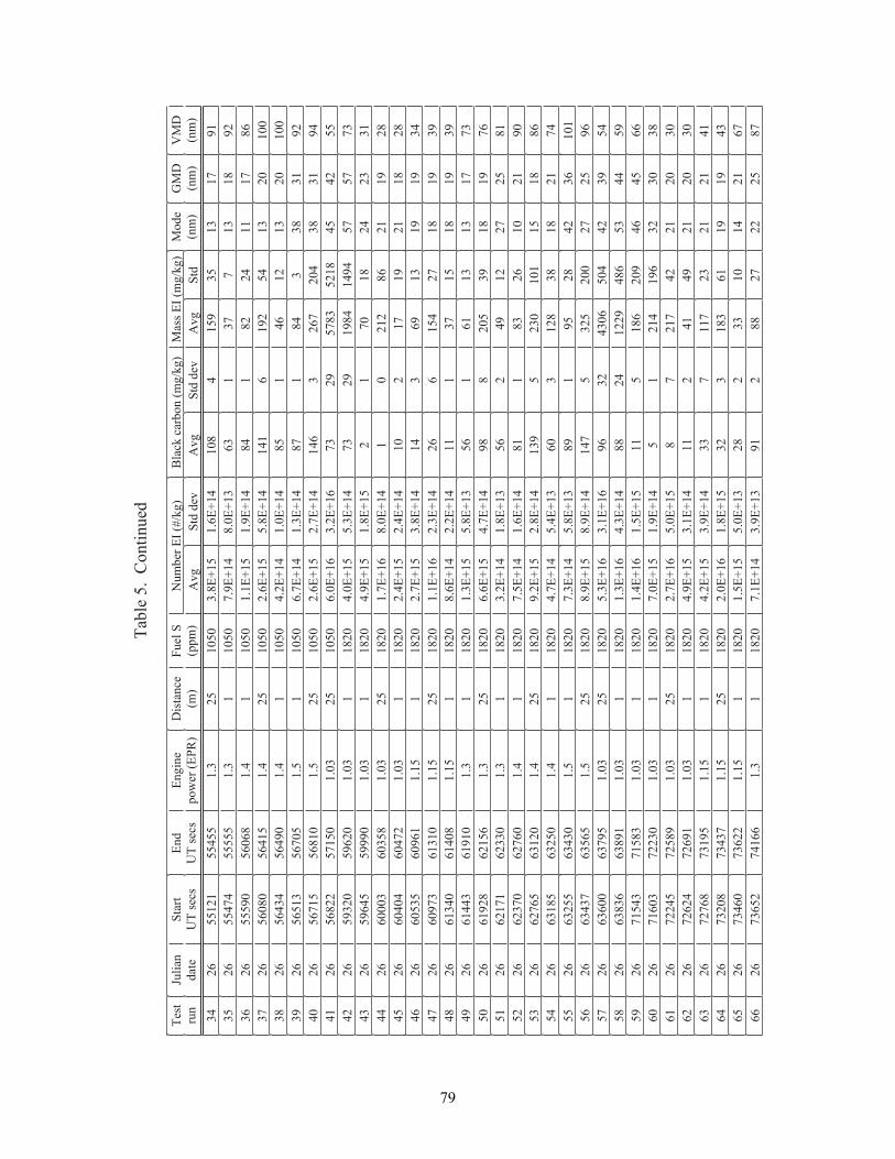
79

deu nitnoC  .5 elba

T

) gk/ gm( I

E  s saM

)gk / gm(  n obrac  k ca l

B)g k/#(  I

E rebmu

Ntse

Tnur

nailuJetad

tratSsce s 

TU

dnE

s ces TU

en ignE

)RP

E( r ew op

ecnat siD

)m(

S l euF)

mpp (dtS

gvA

v ed dtSg v

Av ed  dt S

gvA

ed oM

)m n(

DMG

)m n(

DMV

)mn (

1971

315 3

9 514

8 014 1+

E6 .15 1+

E8 .30 501

523. 1

5545512155

6243

2981

317

731

3 631+

E0 .84 1+

E9 .7050 1

13.1

5555547455

6253

687 1

1 142

281

4 841+

E9 .15 1+

E1 .1050 1

14.1

8606509555

6263

00 102

314 5

2 916

14 14 1+

E8 .55 1+

E 6. 20 501

524.1

5146508065

6273

0 010 2

3 121

641

5841 +

E0 .14 1+

E2 .40 50 1

14.1

0946543465

6283

2913

833

481

7841 +

E3 .14 1+

E7 .60 50 1

15.1

5076531565

6293

4 913

8340 2

7 623

64 14 1+

E 7.251+

E 6. 20 5 01

525. 1

0186551765

6204

552 4

5 481 25

3 8759 2

3 761+

E2 .36 1+

E0 .6050 1

5230.1

0517522865

6214

3775

7549 4 1

4 8919 2

374 1+

E3 .55 1+

E0 .40 281

130.1

0269502395

6224

133 2

4 281

071

251 +

E 8. 151+

E9 .402 81

130.1

0999554695

6234

8 291

1268

21 20

141+

E 0. 861+

E 7. 10281

5230.1

8530630006

6244

8281

129 1

712

014 1+

E4 .251+

E 4. 20281

130.1

2740640406

6254

439 1

9131

9 63

4141+

E8.351 +

E7 .20281

151.1

1690653506

6264

9 391

8172

4 5 16

6241+

E 3. 261 +

E1 .10281

5251 .1

0131637906

6274

9 391

815 1

731

114 1+

E 2.241 +

E6 .80281

151.1

804 1604 316

6284

377 1

3 131

161

6 531+

E8 .551+

E3.10281

13.1

0191634416

6294

6 791

8193

50 28

8 941 +

E 7. 451+

E6.60281

523.1

6512682916

6205

1 852

7221

9 42

6531+

E 8.141+

E2.30281

13.1

0332617126

6215

0 912

0162

3 81

1841+

E6.141+

E5.70281

14.1

0672607326

6225

688 1

5 11 01

0325

9 314 1+

E8 .251+

E2.90281

524. 1

0 213656726

6235

4 712

8183

82 13

063 1+

E4.541+

E7 .402 81

14. 1

0 523 6581 36

6245

10 163

2482

5 91

983 1+

E8.541+

E3 .702 81

15. 1

0 343 6552 36

6255

6952

720 02

5235

7414 1+

E9.851+

E 9. 802 81

5 25 .1

5653 6734 36

6 26 5

4 593

2 4405

60 3 423

6961+

E1.361 +

E 3. 50 28 1

523 0.1

5973 600 636

6 27 5

954 4

3 56 84

922 142

8841+

E3.461+

E3. 10 28 1

13 0.1

1983 663 836

6 28 5

6654

6490 2

6 815

1151+

E5 .161 +

E4. 10 28 1

130 .1

3851 734 51 7

6 295

830 3

2 36 91

4121

54 1+

E9.151 +

E0 .70 281

130 .1

032 273061 7

6206

030 2

1 224

71 27

85 1+

E0.561+

E7 .20 281

5230 .1

985 275422 7

6216

0302

129 4

142

114 1+

E1.351+

E9.40281

130.1

196 274262 7

6226

1 412

123 2

7 117

334 1+

E9.351+

E2.40281

151.1

591 378672 7

6236

3 49 1

9 116

3813

2351+

E8.161+

E0.20281

5251.1

7343780237

6246

7 612

4101

332

8231+

E0 .551+

E5.10281

151 .1

2263706437

6256

7 852

2272

882

1931+

E9.341+

E1.70281

13.1

6614725637

6266

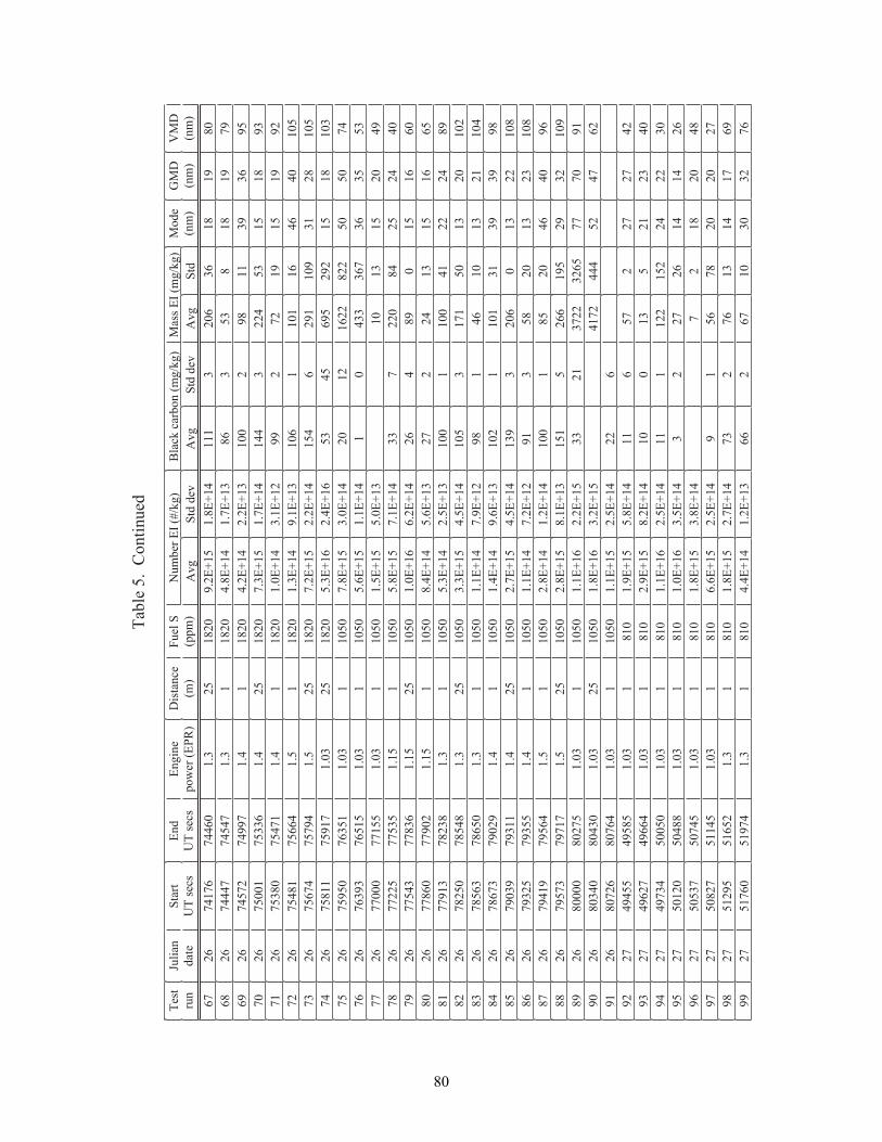
80

deu nitnoC  .5 elba

T

) gk/ gm( I

E  s saM

)gk / gm(  n obrac  k ca l

B)g k/#(  I

E rebmu

Ntse

Tnur

nailuJetad

tratSsce s 

TU

dnE

s ces TU

en ignE

)RP

E( r ew op

ecnat siD

)m(

S l euF)

mpp (dtS

gvA

ved dtSg v

Av ed  dt S

gvA

ed oM

)m n(

DMG

)m n(

DMV

)mn (

0891

816 3

6 023

1 114 1+

E8 .15 1+

E2 .90 281

523. 1

0644767147

6276

9791

818

353

6 831+

E7 .14 1+

E8 .4028 1

13.1

7454774447

6286

5963

931 1

892

0 0131+

E2 .24 1+

E2 .4028 1

14.1

7994727547

6296

3 981

513 5

4 223

44 14 1+

E7 .15 1+

E 3. 70 281

524.1

6335710057

6207

299 1

5 191

272

9921 +

E1 .34 1+

E0 .10 28 1

14.1

1745708357

6217

5 0104

646 1

1 011

6 0131 +

E1 .94 1+

E3 .10 28 1

15.1

4665718457

6227

50 182

1390 1

1 926

45 14 1+

E 2.251+

E 2. 70 2 81

525. 1

4975747657

6237

3 0181

512 92

5965 4

3 561+

E4 .26 1+

E3 .5028 1

5230.1

7195711857

6247

4705

0522 8

2 2612 1

024 1+

E0 .35 1+

E8 .70 501

130.1

1536705957

6257

355 3

6 37 63

33 40

141 +

E 1. 151+

E6 .505 01

130.1

5156739367

6267

940 2

5 131

01 

 31 +

E 0. 551+

E5 .105 01

130.1

5517700077

6277

0442

524 8

0 227

334 1+

E1 .751+

E 8. 50501

151.1

5357752277

6287

066 1

510

984

6241+

E2.661 +

E0.10501

5251.1

6387734577

6297

566 1

5 131

4 22

7 231+

E6 .541 +

E4 .80501

151 .1

2097706877

6208

9 842

2214

0 0 11

00 13 1+

E 5.241+

E3 .50501

13. 1

8328731977

6218

2 010 2

3 105

17 13

50141 +

E 5. 451+

E3.30501

523.1

8458705287

6228

4 011 2

3 101

641

8 921+

E9 .741+

E1.10501

13.1

0568736587

6238

8 993

9313

10 11

20 131+

E 6.941+

E4.10501

14.1

9209737687

6248

80 122

310

6 023

93 14 1+

E5.451+

E7.20501

524.1

1139793097

6258

8 013 2

3 102

853

1921+

E2 .741+

E1.10501

14. 1

5 539752397

6268

690 4

6 402

581

0014 1+

E2.141+

E8 .205 01

15. 1

4 659 7914 97

6278

90 123

92591

6625

15 13 1+

E1.851+

E8 .205 01

5 25. 1

7 179 7375 97

6288

1907

77562 3

22 7312

335 1+

E2.261+

E1.105 01

13 0.1

5720 8000 08

6 29 8

267 4

2 54 44

271 4 

 51+

E2.361 +

E 8. 10 50 1

523 0.1

0340 804 308

6 20 9

  

  

 6

2241+

E5.251+

E1. 10 50 1

13 0.1

4670 862 708

6 21 9

2 472

722

756

1141+

E8 .551 +

E9. 10 18

130 .1

5859 455 49 4

7 229

043 2

1 25

310

014 1+

E2.851 +

E9 .2018

130 .1

466 947269 4

7239

032 2

4 2251

22 11

114 1+

E5.261 +

E1 .1018

130 .1

050 054379 4

7249

6 241

4162

7 22

34 1+

E5.361+

E0.1018

130.1

884 050210 5

7259

840 2

8 12

7 

 4 1+

E8.351+

E8.1018

130.1

547 057350 5

7269

7202

028 7

6 51

941+

E5.251+

E6.6018

130.1

5411572805

7279

9 671

4131

672

3741+

E7 .251+

E8.1018

13.1

2561559215

7289

6 723

0301

762

6631+

E2.141+

E4.4018

13.1

4791506715

7299

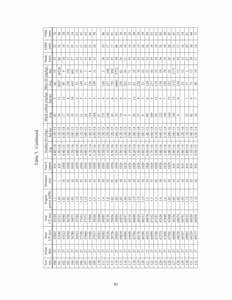
81

deu nitnoC  .5 elba

T

)g k/gm( I

E  ss aM

)gk / gm(  n obrac  k ca l

B)g k/#(  I

E rebmu

Ntse

Tnur

nailuJetad

tratSsce s 

TU

dnE

s ces TU

en ignE

)RP

E( r ew op

ecnat siD

)m(

S l euF)

mpp (dtS

gvA

v ed dtSg v

Av ed  dt S

gvA

ed oM

)m n(

DMG

)m n(

DMV

)mn (

6 723

335 2

663

263 1+

E 1. 141+

E 4. 4018

13 .1

0232558025

72001

8947

0882 26 2

7 2091 1

0 351 +

E1.26 1+

E4.101 8

130.1

3372504525

72101

828 1

8 19

9 43 1

7 141 +

E5. 451 +

E9.6050 1

0 130.1

0856532355

72201

9271

7165 1

0 314

916 1+

E1.161+

E 6. 30 501

5330.1

0576549565

72301

4352

721 06

54481

5 351+

E0.36 1+

E2 .1050 1

0 130.1

5796508765

72401

3671

2161

352

3 331+

E0.74 1+

E4 .6050 1

0 151.1

4817531965

72501

1 471

717 4

9 415

1351+

E 1. 161+

E 2. 205 01

535 1.1

3347589175

72601

3602

517

153

4221 +

E9.74 1+

E0.40 50 1

015 1.1

3757506475

72701

6833

938

6 213

4 1131 +

E4.14 1+

E7.60 50 1

013.1

4097509675

72801

876 1

5 113

99 15

40141+

E 5. 661 +

E2. 105 01

533.1

0628571975

72901

  

  

 2

7931+

E 3. 341 +

E2. 60501

013.1

0438538285

72011

6853

633

0 314

7 313 1+

E5.14 1+

E5.50501

014.1

5058558385

72111

5871

516 41

73 25

64141+

E 5. 261+

E1.10501

534.1

0178562585

72211

1 971

51493

85 76

2 451+

E 2. 761+

E5.80501

5330.1

6588565785

72311

3684

45277 5

66 445

535 1+

E0.26 1+

E3.30501

013 0.1

4309550985

72411

034 2

6 236

85 26

0 141+

E2.861+

E9.10281

0130.1

5705603646

725 11

929 1

1 254

1625

951+

E3.361+

E6.30281

5330.1

7355669056

726 11

9 281

9117

2 51

94 1+

E 9.261+

E1.10281

0130.1

0175600656

72711

9 461

6153

3831

0241+

E 8.141+

E2.90281

0151.1

0506608756

72811

839 1

9 107

42 24

7 241+

E 0. 461+

E 3.10281

535 1.1

81 366671 66

72911

8 542

5222

3 55

831 +

E 8. 141+

E 4. 4028 1

015 1. 1

31 5660 43 66

72021

9 843

3332

4 216

9931 +

E 4. 141+

E 0. 6028 1

013 .1

07 8665 3 566

72121

3681

816 5

7 326

00141 +

E6.461 +

E7. 10 28 1

533. 1

2 61760 9 866

7222 1

369 1

8 123

47 121

0531+

E 1.441 +

E9 .50 2 81

013. 1

7 52766 8 176

7 232 1

395 3

6 391

81 15

22121+

E 4.941 +

E0 .50 2 81

014. 1

8 347 63 7 276

7 242 1

8 681

819 7

8 327

04 141+

E 1. 46 1+

E4.102 81

5 34. 1

0467 606476

7 2521

546 2

9 255

22 131

44 161 +

E 0. 26 1+

E0.702 81

0 13 0.1

0087650776

726 21

343 3

6 377 11

2 71131

44 15 1+

E 0. 26 1+

E0.2018

0 13 0.1

6528608086

727 21

3 37 1

8 171

41 14

451+

E8. 161+

E5.2018

5330.1

4768607286

728 21

4 36 1

5 121

53 

 41+

E2. 251+

E4.3018

0130.1

1978670786

729 21

1892

722

737

523 1+

E1.141+

E4.3018

0151.1

53296569 86

72031

4 803

9271

378

5 44 1+

E 9.26 1+

E1.1018

5351.1

95 396952 96

72131

2 761

719 1

947

814 1+

E 3.451+

E5.3018

0151.1

83 596773 96

72231

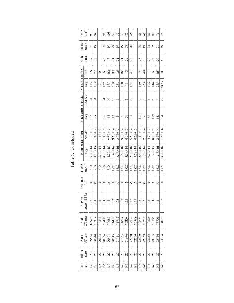
82

dedulcnoC  . 5 elba

T

)g k/gm( I

E  ss aM

)gk / gm(  n obrac  k ca l

B)g k/#(  I

E rebmu

Ntse

Tnur

nailuJetad

tratSsce s 

TU

dnE

s ces TU

en ignE

)RP

E( r ew op

ecnat siD

)m(

S l euF)

mpp (dtS

gvA

v ed dtSg v

Av ed  dt S

gvA

ed oM

)m n(

DMG

)m n(

DMV

)mn (

1 953

4381

51 113

393 1+

E 3. 141+

E 6. 5018

013 .1

6299646596

72331

9981

312 2

56143

8 341 +

E1.15 1+

E5.401 8

5 33.1

8420702007

72431

  

 0

0 

 31 +

E1.14 1+

E6.501 8

0 13.1

4130727207

72531

597 3

3 46

72 143

8331+

E 1. 141 +

E9. 40 18

014.1

2840762307

72631

50 191

3166 1

7 810 1

413 1+

E8.95 1+

E2.401 8

5 34.1

7860740507

72731

8392

139 8

8055 1

3 141+

E6.96 1+

E4 .1028 1

0 130.1

6341754707

72831

0 391

1262

82 24

551+

E 0. 361+

E 6. 302 81

533 0.1

2171785417

72931

1391

129 8 1

0 212

541 +

E0.96 1+

E8.10 28 1

013 0.1

4381733717

72041

088 2

9 251

145

9231 +

E2.44 1+

E2.50 28 1

015 1.1

8032767917

72141

5 402

0214

7616

1341+

E 5. 561 +

E3. 202 81

5351.1

2352703327

72241

  

  

  

 31+

E 5. 441 +

E6. 40281

0151.1

8852706527

72341

6852

524 1

9 312

4 014 1+

E1.15 1+

E4.20281

013.1

6982702627

72441

6 691

8184

53 25

6 941+

E 9. 261+

E5.10281

533.1

2123793927

72541

2 832

0231

60 13

8 831+

E 7. 441+

E7.90281

013 .1

5233724237

72641

7 823

636

4 413

91 13 1+

E7.85 1+

E2.10281

014 .1

3053756337

72741

671 2

0 27 61

5526

3 3141+

E9.261+

E4.10281

534.1

4073762537

72841

679 5

6 60

3 34 52 2

4 761+

E5.161+

E9.30281

0130.1

0204746737

729 41

83

secidnI noissimE reb

muN elci traP 757-

B f o yram

muS  .6 elbaT

ruflu s leuf mpp 02 81

rufl us l euf mp p 0 501

ruflus  leuf mpp 018

51e1 x IE reb

mun51e1 x I

E rebmun

51e 1 x IE  re b

munelp

maSeborpecnatsid

)m(

enignE

erusserpoitar)RP

E(a

mgiSnaide

Megarev

AN

amgiS

naideM

e garevA

Na

m giSnaide

Megarev

AN

85. 498.7

10.87

98.387 .1

41.48

76.944.01

61.1101

30.11

70.388.3

08.34

7 0.621. 4

58 .53

 38.8

38.81

51.1 

55.187.1

1 8.14

78.059. 0

50 .14

99. 298.2

30.34

3.1 

33 .084.0

94 .04

87. 07 2.0

06.04

 04.4

04.41

4.1 

53 .073.0

73 .02

33. 015.0

1 5.02

 97.3

97.31

5.1 

59.4152.62

3 5.7 26

64.4106. 81

12 .123

11.1106.11

55.515

30.101

71.44 0.1

19. 24

65.125.1

2 5.12

68.516.4

89.54

51.1 

27 .09 7.0

80. 14

31.017.0

1 7.02

62.566.0

56.33

3.1 

65.098.0

98.02

 55.0

55.01

13.445.3

45.32

4.1 

4 7.9 104. 83

30 .934

06.4200.12

60.623

  

  

30.152

08 .503.61

03.612

90.414.8

14.82

  

  

51.1 

93.196.8

96.82

31. 029.3

29.32

  

  

3.1 

15.125.8

25.82

20. 009.2

09.22

  

  

4.1 

34.15 1.8

51. 82

80.049.2

49.22

  

  

5.1 

31.109.73

09 .732

79.0307.75

07.752

 3.62

3.621

30.153

15.60 3.8 1

03. 812

 08.22

08.221

 02.11

02.111

51.1 

43.15 2.6 1

52. 612

 08.21

08.211

 56.4

56.41

3.1 

 0 3.4 1

03.412

 07.01

07.011

 42.4

42.41

4.1 

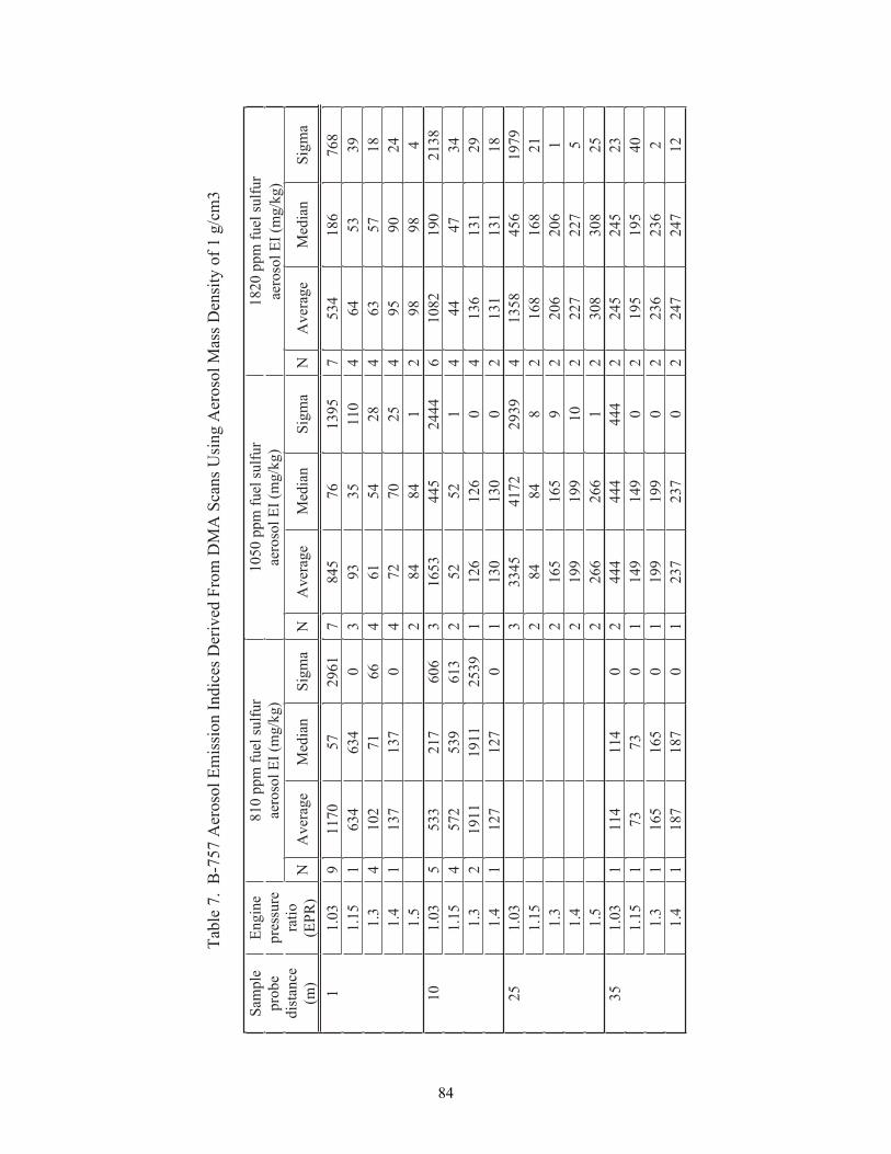
84

3mc/g 1 fo ytisne

D ssaM losore

A gnisU snacS 

AMD 

morF devireD secidnI noissi

mE losore

A 757-B  .7 elba

T

rufl us leuf mp p 0 281

r uf lu s  le uf  mpp  01 8

)gk/ gm( I

E los orearuflus leuf 

mpp 050 1)gk/g

m(  IE l osorea

)gk/gm( I

E losoreaelp

maSeborpecnatsid

)m(

enignE

erusserpoitar)RP

E(a

mgiSnai de

Megarev

AN

amgiS

naideM

egare vA

Na

mgiSnai de

Megarev

AN

867681

4357

5 93167

5487

16927 5

07119

30.11

9335

464

01153

393

0436

4361

51.1 

817 5

3 64

8 24 5

164

6617

2014

3.1 

4209

594

5207

274

0731

7311

4.1 

489

892

148

482

  

  

5.1 

8312091

28 016

4442544

35613

606712

3355

30.101

437 4

4 44

125

2 52

316935

2754

51.1 

921 31

6314

062 1

6 211

93521191

11912

3.1 

81131

1312

003 1

0 311

0721

7211

4.1 

97916 54

85314

93922714

54333

  

  

30.152

12861

8612

848

482

  

  

51.1 

1602

6022

95 61

5612

  

  

3.1 

57 22

7 222

0 19 91

9912

  

  

4.1 

5 2803

8032

16 62

6622

  

  

5.1 

32542

54 22

444444

4442

0411

4111

30.153

045 91

5 912

0941

9411

037

371

51.1 

2632

63 22

0991

9911

0561

5611

3.1 

2174 2

74 22

0732

7321

0781

7811

4.1 

85

noitprosbA gnis

U ataD rete

mortcepS noitprosbA tooS elcitraP 

morF devireD secidnI noissi

mE nobra

C kcalB 757-

B  .8 elbaT

g/2m 7 fo ycneiciff

E

ruf lu s leuf m pp  018

)g k/gm( I

E  n obra c kcalB

r uf lu s  leuf mpp 05 01

) gk/gm( I

E nobrac kcalB

ruflus leuf mpp  0281

)gk/ gm( I

E nobrac  kcalB

elpmaSeborpecnatsid

)m(

enignE

erusserpoitar)RP

E(a

m giSnaide

Megarev

AN

am giS

naideM

egarevA

Na

m giSnaide

Megarev

AN

6311

927

218

317

6111

619

30.11

1112

1 24

472

823

  

  

51.1 

9 117

2 74

1218

184

2 346

154

3.1 

910 9

584

888

194

  

  

4.1 

118 9

892

939

392

  

  

5.1 

6 521

2 46

1153

923

6676

274

30.101

0 102

9 13

792

922

3142

824

51.1 

4239

584

216 01

6 012

71101

1012

3.1 

4021

0212

473 1

7311

0608

082

4.1 

4 403

0 44

9483

832

  

  

30.152

592

922

522

222

  

  

51.1 

9501

5012

460 1

6012

  

  

3.1 

4241

2412

5041

0412

  

  

4.1 

5151

1 512

4841

8412

  

  

5.1 

47

72

6 103

032

44

41

30.153

592

922

513

131

854

541

51.1 

689

892

5401

4011

3383

831

3.1 

77 31

73 12

5641

6411

  

  

4.1 

86

egnaR eziS 

mn 042 ot 9 revO 

AMD 

morF devireD srete

maiD nae

M emu lo

V dna naeM cirte

moeG 757-

B fo yram

mu S  .9 elbaT

r uflus  le uf mpp 018

sretemonan

ru flus  l eu f mpp 0501

sretemona n

ruflus leuf mpp 02 81

sretemo nan

elpmaSeborpecnatsid

)m(

enignE

erusserpoitar)RP

E(a

mgiSD

MV

amgiS

DMG

NamgiS

DMV

amgiS

DMG

NamgiS

DMV

amgiS

DMG

N

916 4

5143

712

4591

537

2 234

8182

930.1

151

541

024

4194

591

30

3 50

141

51.1 

60 8

412

441

983

024

3186

772

43.1

 9

8 88

424

989

0152

4 

  

  

4.1 

3301

383

23

496

532

086

022

15.1

 8 1

2451

926

  

6103

333

4742

545

30.101

6 136

632

3 

 2

912

996

6163

451.1

 21

087

524

  

033

13

3902

942

3.1 

409

243

2 

 0

531

059

073

14.1

 53

3501

4 24

5105

3 173

3 

  

  

30.152

31 4

091

201

452

712

  

  

 51.1

 3

8 70

912

879

291

2 

  

  

3.1 

59 8

081

26

4 011

122

  

  

 4.1

 6

1 012

7 22

011 01

123

2 

  

  

5.1 

103

091

244

060

712

033

071

130.1

535

241

022

014

071

10

480

031

51.1 

24 6

091

20

870

611

099

081

13.1

 5

2 72

022

058

071

10

5010

911

4.1 

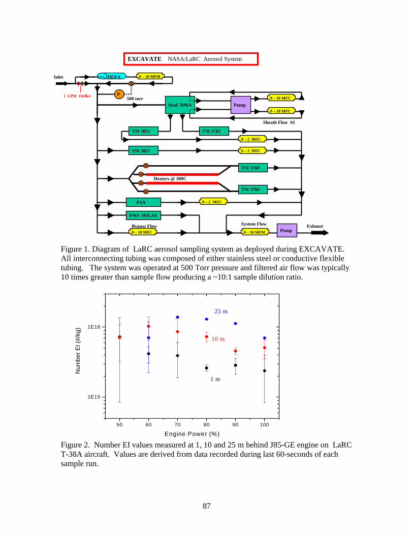
87

Figure 1. Diagram of LaRC aerosol sampling system as deployed during EXCAVATE. All interconnecting tubing was composed of either stainless steel or conductive flexible tubing. The system was operated at 500 Torr pressure and filtered air flow was typically 10 times greater than sample flow producing a ~10:1 sample dilution ratio. Figure 2. Number EI values measured at 1, 10 and 25 m behind J85-GE engine on LaRC T-38A aircraft. Values are derived from data recorded during last 60-seconds of each sample run.

EXCAVATE NASA/LaRC Aerosol System

Inlet

Dual DMA Pump

HEPA

1 LPM Orifice P

HEPA

Sheath Flow #2

500 torr

TSI 3025 TSI 3762

TSI 3022

Pump Exhaust

0 – 10 MFM

0 – 10 MFC

0 – 10 MFC

0 – 2 MFC

0 – 2 MFC 0 – 2 MFC

0 – 10 MFM 0 – 10 MFC

Bypass Flow System Flow

PMS HSLAS

TSI 3760

TSI 3760

Heaters @ 300C

PSAP

0 – 2 MFC

50 60 70 80 90 100

1E15

1E16

25 m

10 m

1 m

Num

ber

EI (

#/kg

)

Engine Power (%)

88

Figure 3. Aerosol mass EI values derived from DMA size distribution scans performed on samples collected at 1 and 10 m behind T-38A exhaust plane. Figure 4. Geometric mean diameters derived from DMA size distribution scans performed on samples collected at 1 and 10 m behind T-38A exhaust plane.

50 60 70 80 90 100

0

50

100

150

200

250

300

350

400

450

500

550

10 m

1 m

Mas

s E

I (m

g/kg

)

Engine Power (%)

50 60 70 80 90 100

20

22

24

26

28

30

32

34

36

10 m

1 m

Geo

met

ric M

ean

Dia

met

er (

nm)

Engine Power

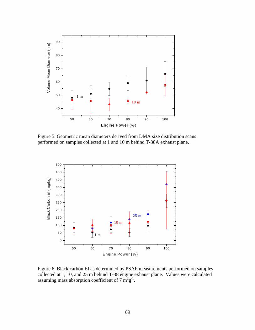
89

Figure 5. Geometric mean diameters derived from DMA size distribution scans performed on samples collected at 1 and 10 m behind T-38A exhaust plane. Figure 6. Black carbon EI as determined by PSAP measurements performed on samples collected at 1, 10, and 25 m behind T-38 engine exhaust plane. Values were calculated assuming mass absorption coefficient of 7 m2g-1.

50 60 70 80 90 100

40

50

60

70

80

90

10 m

1 m

Vol

ume

Mea

n D

iam

eter

(nm

)

Engine Power (%)

50 60 70 80 90 100

0

50

100

150

200

250

300

350

400

450

500

25 m

10 m

1 m

Bla

ck C

arbo

n E

I (m

g/kg

)

Engine Power (%)

90

50 60 70 80 90 1000

5

10

15

20

25

32:1

16:1

8:1

Em

issi

on In

dex

x 1E

15 (

#/kg

)

Engine Power (%)

Figure 7. Aerosol number EI values for samples collected 1 m behind T-38 using dilution ratios of 8:1, 16:1 and 32:1, as determined from CO2 mixing ratio measurements. Figure 8. Number EI values for various engine power settings as determined at 1, 10, 25 and 35 m sampling distances for cases when aircraft was burning 1820 ppmS fuel.

1.0 1.1 1.2 1.3 1.4 1.5

0.1

1

10

35 m

25 m

10 m1 m

Aer

osol

Num

ber

EI x

E15

/kg

Engine Pressure Ratio

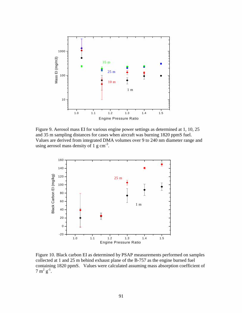
91

Figure 9. Aerosol mass EI for various engine power settings as determined at 1, 10, 25 and 35 m sampling distances for cases when aircraft was burning 1820 ppmS fuel. Values are derived from integrated DMA volumes over 9 to 240 nm diameter range and using aerosol mass density of 1 g cm-3. Figure 10. Black carbon EI as determined by PSAP measurements performed on samples collected at 1 and 25 m behind exhaust plane of the B-757 as the engine burned fuel containing 1820 ppmS. Values were calculated assuming mass absorption coefficient of 7 m2 g-1.

1.0 1.1 1.2 1.3 1.4 1.5

10

100

1000

35 m

25 m

10 m

1 m

Mas

s E

I (m

g/m

3)

Engine Pressure Ratio

1.0 1.1 1.2 1.3 1.4 1.5-20

0

20

40

60

80

100

120

140

160

25 m

1 m

Bla

ck C

arbo

n E

I (m

g/kg

)

Engine Pressure Ratio

92

Figure 11. Geometric mean diameters derived from DMA size distribution scans performed on samples collected at 1 and 25 m behind B-757 exhaust plane as engine burned fuel containing 1820 ppmS. Figure 12. Volume mean diameters derived from DMA size distribution scans performed on samples collected at 1 and 25 m behind B-757 exhaust plane as engine burned fuel containing 1820 ppmS.

1.0 1.1 1.2 1.3 1.4 1.510

15

20

25

30

35

40

45

50

25 m

1 m

Geo

met

ric M

ean

Dia

met

er (

nm)

Engine Pressure Ratio

1.0 1.1 1.2 1.3 1.4 1.510

20

30

40

50

60

70

80

90

100

110

25 m

1 m

Vol

ume

Mea

n D

iam

eter

(nm

)

Engine Pressure Ratio

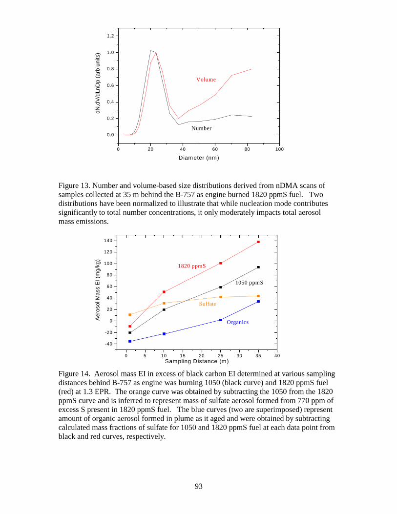
93

Figure 13. Number and volume-based size distributions derived from nDMA scans of samples collected at 35 m behind the B-757 as engine burned 1820 ppmS fuel. Two distributions have been normalized to illustrate that while nucleation mode contributes significantly to total number concentrations, it only moderately impacts total aerosol mass emissions. Figure 14. Aerosol mass EI in excess of black carbon EI determined at various sampling distances behind B-757 as engine was burning 1050 (black curve) and 1820 ppmS fuel (red) at 1.3 EPR. The orange curve was obtained by subtracting the 1050 from the 1820 ppmS curve and is inferred to represent mass of sulfate aerosol formed from 770 ppm of excess S present in 1820 ppmS fuel. The blue curves (two are superimposed) represent amount of organic aerosol formed in plume as it aged and were obtained by subtracting calculated mass fractions of sulfate for 1050 and 1820 ppmS fuel at each data point from black and red curves, respectively.

0 20 40 60 80 100

0.0

0.2

0.4

0.6

0.8

1.0

1.2

Number

Volume

dN,d

V/d

LnD

p (a

rb u

nits

)

D iameter (nm)

0 5 10 15 20 25 30 35 40

-40

-20

0

20

40

60

80

100

120

140

Organics

Sulfate

1050 ppmS

1820 ppmS

Aer

osol

Mas

s E

I (m

g/kg

)

Sampling Distance (m)

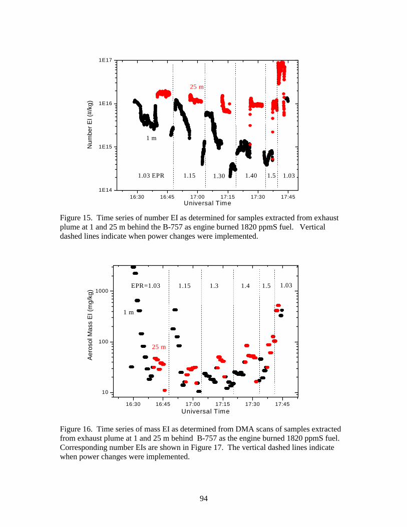
94

Figure 15. Time series of number EI as determined for samples extracted from exhaust plume at 1 and 25 m behind the B-757 as engine burned 1820 ppmS fuel. Vertical dashed lines indicate when power changes were implemented. Figure 16. Time series of mass EI as determined from DMA scans of samples extracted from exhaust plume at 1 and 25 m behind B-757 as the engine burned 1820 ppmS fuel. Corresponding number EIs are shown in Figure 17. The vertical dashed lines indicate when power changes were implemented.

16:30 16:45 17:00 17:15 17:30 17:451E14

1E15

1E16

1E17

1.031.51.401.301.151.03 EPR

25 m

1 m

Num

ber

EI (

#/kg

)

Universal Time

16:30 16:45 17:00 17:15 17:30 17:45

10

100

1000

1 m

25 m

1.031.51.41.31.15EPR=1.03

Aer

osol

Mas

s E

I (m

g/kg

)

Universal Time

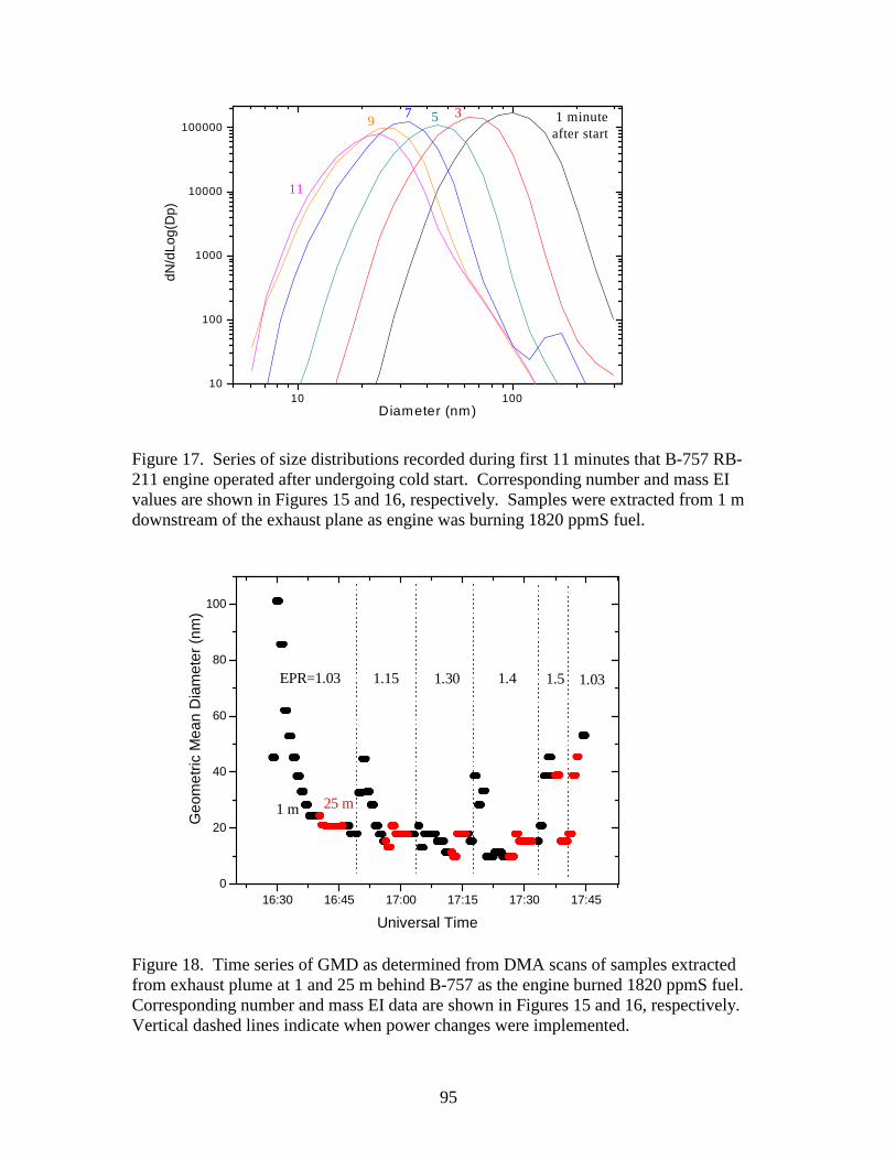
95

Figure 17. Series of size distributions recorded during first 11 minutes that B-757 RB-211 engine operated after undergoing cold start. Corresponding number and mass EI values are shown in Figures 15 and 16, respectively. Samples were extracted from 1 m downstream of the exhaust plane as engine was burning 1820 ppmS fuel. Figure 18. Time series of GMD as determined from DMA scans of samples extracted from exhaust plume at 1 and 25 m behind B-757 as the engine burned 1820 ppmS fuel. Corresponding number and mass EI data are shown in Figures 15 and 16, respectively. Vertical dashed lines indicate when power changes were implemented.

10 10010

100

1000

10000

100000

11

97 5 3 1 minute

after start

dN/d

Log(

Dp)

D iameter (nm)

16:30 16:45 17:00 17:15 17:30 17:450

20

40

60

80

100

25 m1 m

1.031.51.41.301.15EPR=1.03

Geo

met

ric M

ean

Dia

met

er (

nm)

Universal Time

96

APPENDIX E: Improved Nanometer Aerosol Size Analyzer H.-S Han and D. Y. H. Pui

Particle Technology Laboratory Mechanical Engineering Department

University of Minnesota, Minneapolis, MN

7.1 Introduction

In this chapter, an improved version of Nanometer Aerosol Size Analyzer (nASA)

is described. The hardware of this nASA is redesigned so that it is much smaller and

robust than the previous one. Base on the previous extensive simulation study for the

data inversion algorithms, MICRON is proved to provide the most accurate particle size

distribution function with reasonable speed and stability. Therefore, MICRON is

incorporated into the inversion software of this nASA. Figure 7.1 shows the picture of

the modified nASA. The system was calibrated carefully for its delay time, and

evaluated extensively using sodium chloride and silver particles. Finally, the system was

used in the EXperiment to Characterize Aircraft Volatile Aerosol and Trace species

Emissions (EXCAVATE) workshop. The purpose of this workshop, which was

organized by NASA Langley Research Center in Hampton, VA, is to evaluate the

particles emitted from T-38 and Boeing 757 aircraft engines. The workshop was

conducted in Hampton, VA from January 15th to 29th, 2002. Experimental setup and

results from this field trip are presented in the following sections.

97

Fig

ure

7.1

Im

prov

ed N

anom

eter

Aer

osol

Siz

e A

naly

zer

98

7.2 Experimental Setup

The experimental setup for this field study is shown in Figure 7.2. Aircraft-

generated particles were drawn into a sampling probe which is developed by NASA

Langley Research Center. After entering the sampling probe, the aerosols were diluted

and quenched by dilution air, which in this field study is dry Nitrogen. In order to

observe the aerosol growing characteristics and the effects of the ambient dilution,

different dilution ratios were implemented. Different dilution ratio of the sample can be

archived by adjusting the flow rate of Nitrogen. Depending on the engine power and the

probe distance, the temperature of the aerosol sample exited the sampling probe was in

the range of 30 to 80 ˚C. After the dilution, the aerosol samples were then distributed to

aerosol instruments by 40 ft of stainless tubing. The losses in the tubing were carefully

evaluated in the laboratory using the NaCl particles. Some of the aerosol samples were

also heated to 300 ˚C before they were drawn into the nASA. Doing this will vaporize

the volatile particles and the only remaining particles are non-volatile particles. The flow

rate used by the nASA was 1.5 lpm and controlled by a vacuum pump and a valve.

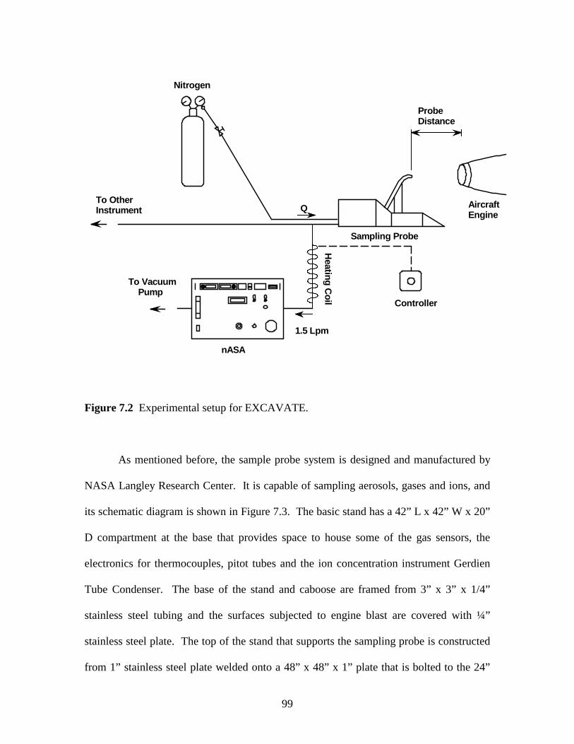
99

Nitrogen

ProbeDistance

To OtherInstrument

To Vacuum Pump

nASA

Controller

1.5 Lpm

Sampling Probe

AircraftEngine

Q

Heating

Coil

Figure 7.2 Experimental setup for EXCAVATE.

As mentioned before, the sample probe system is designed and manufactured by

NASA Langley Research Center. It is capable of sampling aerosols, gases and ions, and

its schematic diagram is shown in Figure 7.3. The basic stand has a 42” L x 42” W x 20”

D compartment at the base that provides space to house some of the gas sensors, the

electronics for thermocouples, pitot tubes and the ion concentration instrument Gerdien

Tube Condenser. The base of the stand and caboose are framed from 3” x 3” x 1/4”

stainless steel tubing and the surfaces subjected to engine blast are covered with ¼”

stainless steel plate. The top of the stand that supports the sampling probe is constructed

from 1” stainless steel plate welded onto a 48” x 48” x 1” plate that is bolted to the 24”

100

high base of the stand. The sampling probe system weight about 2000 lbs. To further

prevent it moving while the engine is running, the stand has a trailer hitch on the front

which can be bolted to a hard point in the tarmac. Figure 7.4 shows the close look of the

sampling probe. The biggest stainless steel tubing is used for gas sampling. The

dynamic pressure is measured by a pitot tube which is the smallest tubing shown in the

photo. Between the gas sampling tube and pitot tube is the aerosol sampling tube. At the

tip of this aerosol sampling tube, there is a critical orifice and its performance is

evaluated in Particle Technology Laboratory, University of Minnesota, MN using NaCl.

The calibration curve is presented in next section. Underneath the three tubings is the

Gerdien Condenser. Thermocouples were also mounted to the support (not shown in the

photo). Some of the gas instruments are located in the caboose, as shown in Figure 7.5.

After the dilution, the samples were distributed to aerosol, gas and ion measurement

systems which were located in several trailers, as shown in Figure 7.6.

Emissions of sulfur oxides (SOx) are primary determined by the sulfur content of

the jet fuel. These sulfur oxides are mainly in the form of SO2, which will oxidize and

condense on the background aerosols, at the combustor exit. In order to verify how

efficiency the fuel sulfur content (FSC) is converted to sulfate particles, in the form of

SO3 and H2SO4, in the engine and near and far field, a parameter ξ is defined. The value

of ξ is believed to be determined largely by the sulfur oxidation mechanisms within the

combustor, turbine and exhaust nozzle. Observations taken from NASA SUbsonic

aircraft Contrail and Cloud Effects Special Study (SUCCESS) show that ξ doesn’t have

strong dependence with FSC (Miake-Lye et al., 1998). In another study, SULFUR which

101

conducted by German agency the Deutsches Zentrum für Luft- und Raumfahrt (DLR),

indicates that ξ decreases with the increase of FSC (Schröder et al., 1998). In order to

investigate whether FSC will influence the amount of sulfate particles generated, fuels

with 810, 1050 and 1820 ppm of sulfur content were used in the experiment.

Caboose

72"x42"x42"42"x42"x20"

Flow SpoilerFlow Spolier

Flow Spoiler

Sampling Probe

Support

Figure 7.3 Sampling probe system.

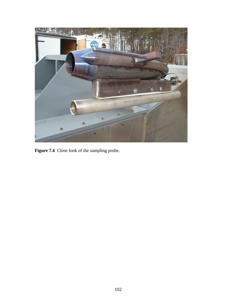
102

Figure 7.4 Close look of the sampling probe.

103

Figure 7.5 Some gas instruments located in the caboose.

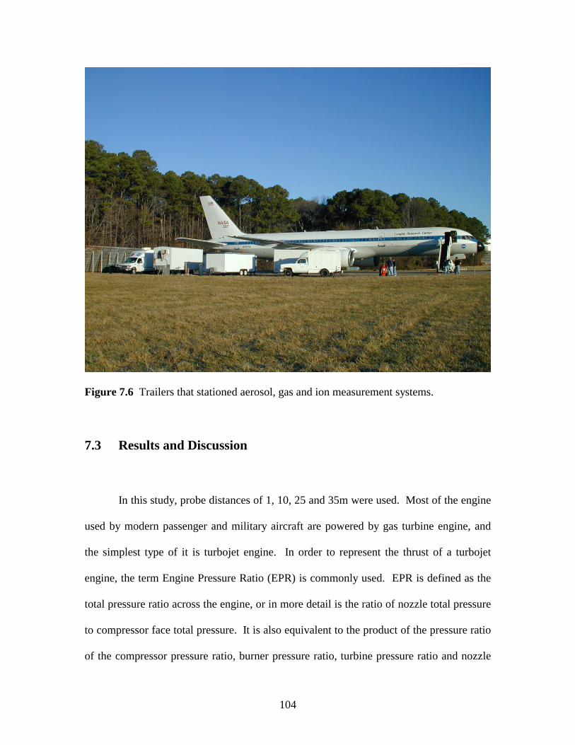
104

Figure 7.6 Trailers that stationed aerosol, gas and ion measurement systems.

7.3 Results and Discussion

In this study, probe distances of 1, 10, 25 and 35m were used. Most of the engine

used by modern passenger and military aircraft are powered by gas turbine engine, and

the simplest type of it is turbojet engine. In order to represent the thrust of a turbojet

engine, the term Engine Pressure Ratio (EPR) is commonly used. EPR is defined as the

total pressure ratio across the engine, or in more detail is the ratio of nozzle total pressure

to compressor face total pressure. It is also equivalent to the product of the pressure ratio

of the compressor pressure ratio, burner pressure ratio, turbine pressure ratio and nozzle

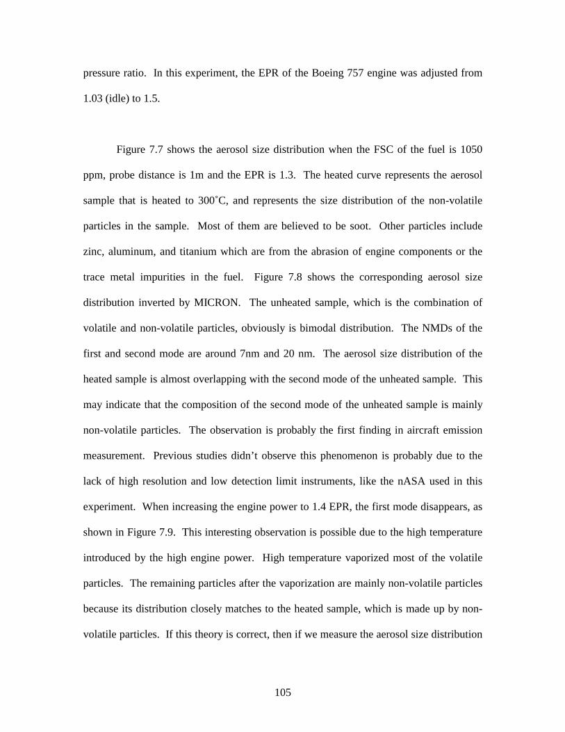
105

pressure ratio. In this experiment, the EPR of the Boeing 757 engine was adjusted from

1.03 (idle) to 1.5.

Figure 7.7 shows the aerosol size distribution when the FSC of the fuel is 1050

ppm, probe distance is 1m and the EPR is 1.3. The heated curve represents the aerosol

sample that is heated to 300˚C, and represents the size distribution of the non-volatile

particles in the sample. Most of them are believed to be soot. Other particles include

zinc, aluminum, and titanium which are from the abrasion of engine components or the

trace metal impurities in the fuel. Figure 7.8 shows the corresponding aerosol size

distribution inverted by MICRON. The unheated sample, which is the combination of

volatile and non-volatile particles, obviously is bimodal distribution. The NMDs of the

first and second mode are around 7nm and 20 nm. The aerosol size distribution of the

heated sample is almost overlapping with the second mode of the unheated sample. This

may indicate that the composition of the second mode of the unheated sample is mainly

non-volatile particles. The observation is probably the first finding in aircraft emission

measurement. Previous studies didn’t observe this phenomenon is probably due to the

lack of high resolution and low detection limit instruments, like the nASA used in this

experiment. When increasing the engine power to 1.4 EPR, the first mode disappears, as

shown in Figure 7.9. This interesting observation is possible due to the high temperature

introduced by the high engine power. High temperature vaporized most of the volatile

particles. The remaining particles after the vaporization are mainly non-volatile particles

because its distribution closely matches to the heated sample, which is made up by non-

volatile particles. If this theory is correct, then if we measure the aerosol size distribution

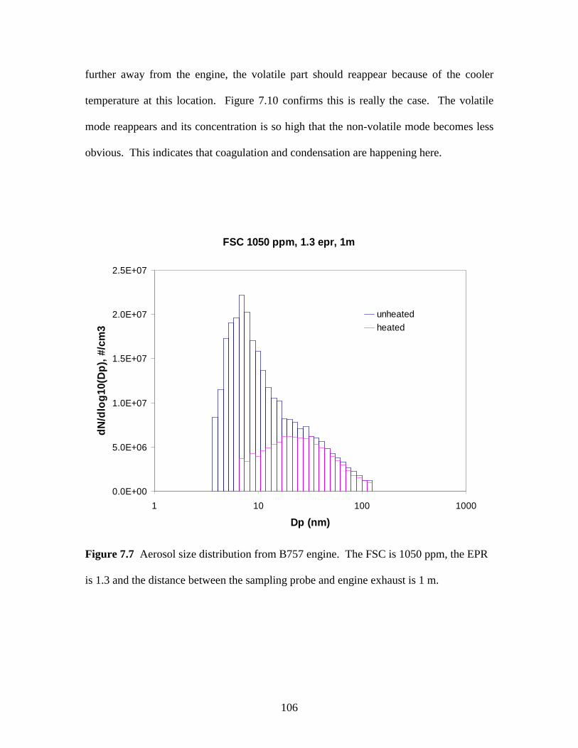
106

further away from the engine, the volatile part should reappear because of the cooler

temperature at this location. Figure 7.10 confirms this is really the case. The volatile

mode reappears and its concentration is so high that the non-volatile mode becomes less

obvious. This indicates that coagulation and condensation are happening here.

FSC 1050 ppm, 1.3 epr, 1m

0.0E+00

5.0E+06

1.0E+07

1.5E+07

2.0E+07

2.5E+07

1 10 100 1000

Dp (nm)

dN

/dlo

g10

(Dp

), #

/cm

3

unheatedheated

Figure 7.7 Aerosol size distribution from B757 engine. The FSC is 1050 ppm, the EPR

is 1.3 and the distance between the sampling probe and engine exhaust is 1 m.

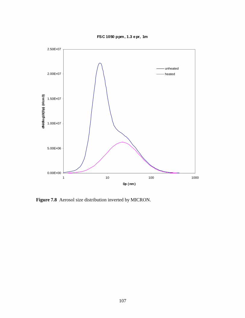
107

FSC 1050 ppm, 1.3 epr, 1m

0.00E+00

5.00E+06

1.00E+07

1.50E+07

2.00E+07

2.50E+07

1 10 100 1000

Dp (nm)

dN/d

log1

0(D

p) (#

/cm

3)

unheated

heated

Figure 7.8 Aerosol size distribution inverted by MICRON.

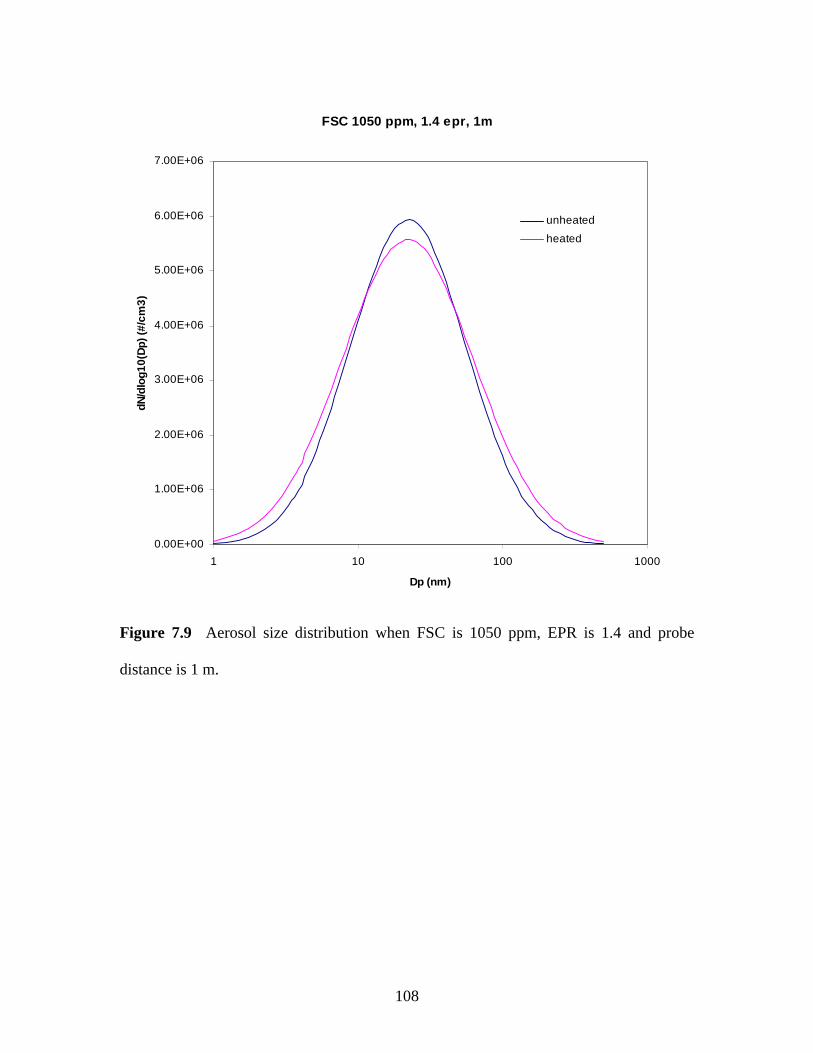
108

FSC 1050 ppm, 1.4 epr, 1m

0.00E+00

1.00E+06

2.00E+06

3.00E+06

4.00E+06

5.00E+06

6.00E+06

7.00E+06

1 10 100 1000

Dp (nm)

dN/d

log1

0(D

p) (#

/cm

3)

unheated

heated

Figure 7.9 Aerosol size distribution when FSC is 1050 ppm, EPR is 1.4 and probe

distance is 1 m.

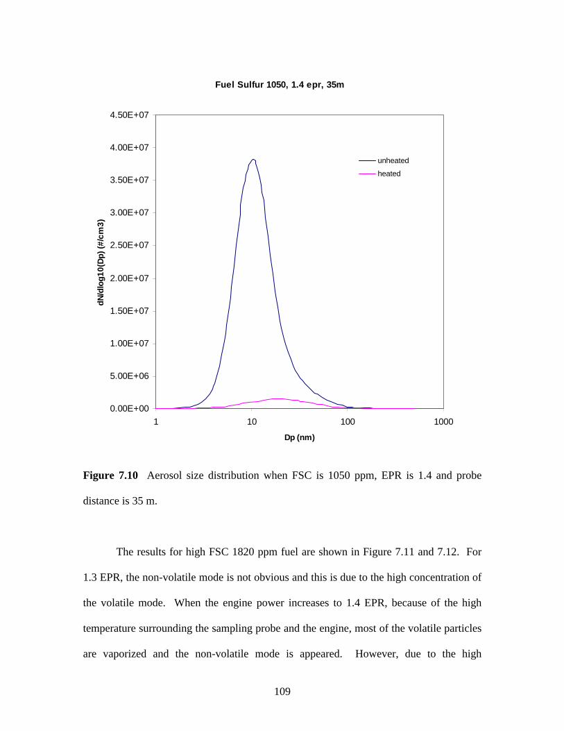
109

Fuel Sulfur 1050, 1.4 epr, 35m

0.00E+00

5.00E+06

1.00E+07

1.50E+07

2.00E+07

2.50E+07

3.00E+07

3.50E+07

4.00E+07

4.50E+07

1 10 100 1000

Dp (nm)

dN/d

log1

0(D

p) (#

/cm

3)

unheated

heated

Figure 7.10 Aerosol size distribution when FSC is 1050 ppm, EPR is 1.4 and probe

distance is 35 m.

The results for high FSC 1820 ppm fuel are shown in Figure 7.11 and 7.12. For

1.3 EPR, the non-volatile mode is not obvious and this is due to the high concentration of

the volatile mode. When the engine power increases to 1.4 EPR, because of the high

temperature surrounding the sampling probe and the engine, most of the volatile particles

are vaporized and the non-volatile mode is appeared. However, due to the high

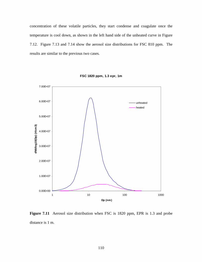
110

concentration of these volatile particles, they start condense and coagulate once the

temperature is cool down, as shown in the left hand side of the unheated curve in Figure

7.12. Figure 7.13 and 7.14 show the aerosol size distributions for FSC 810 ppm. The

results are similar to the previous two cases.

FSC 1820 ppm, 1.3 epr, 1m

0.00E+00

1.00E+07

2.00E+07

3.00E+07

4.00E+07

5.00E+07

6.00E+07

7.00E+07

1 10 100 1000

Dp (nm)

dN

/dlo

g10

(Dp

) (#

/cm

3)

unheated

heated

Figure 7.11 Aerosol size distribution when FSC is 1820 ppm, EPR is 1.3 and probe

distance is 1 m.

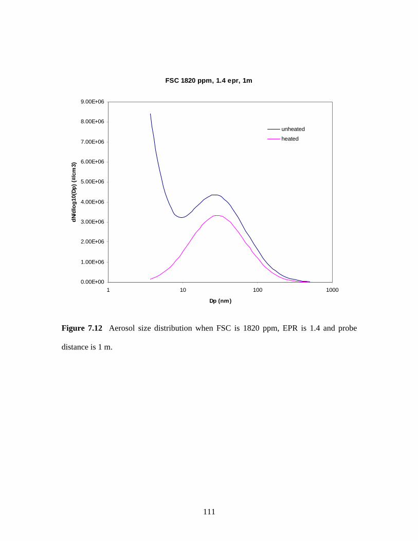
111

FSC 1820 ppm, 1.4 epr, 1m

0.00E+00

1.00E+06

2.00E+06

3.00E+06

4.00E+06

5.00E+06

6.00E+06

7.00E+06

8.00E+06

9.00E+06

1 10 100 1000

Dp (nm)

dN

/dlo

g10

(Dp

) (#

/cm

3)

unheated

heated

Figure 7.12 Aerosol size distribution when FSC is 1820 ppm, EPR is 1.4 and probe

distance is 1 m.

112

FSC 810 ppm, 1.3 epr, 1m

0.00E+00

5.00E+06

1.00E+07

1.50E+07

2.00E+07

2.50E+07

1 10 100 1000

Dp (nm)

dN/d

log1

0(D

p) (#

/cm

3)

unheated

heated

Figure 7.13 Aerosol size distribution when FSC is 810 ppm, EPR is 1.3 and probe

distance is 1 m.

113

FSC 810 ppm, 1.4 epr, 35m

0.00E+00

5.00E+06

1.00E+07

1.50E+07

2.00E+07

2.50E+07

1 10 100 1000

Dp (nm)

dN

/dlo

g10

(Dp

) (#

/cm

3)

unheated

heated

Figure 7.14 Aerosol size distribution when FSC is 810 ppm, EPR is 1.4 and probe

distance is 35 m.

By comparing these three cases, it seems like the modes of non-volatile particles

are quite consistent. All the non-volatile modes have peaks around 20 to 24 nm and

concentrations are in the range of 4x106 to 5x106 #/cm3. This indicates that non-volatile

particle mode of aircraft generated aerosol size distribution is not effected by FSC of the

fuel. However, the amount of sulfur content do influence the amount of volatile particles

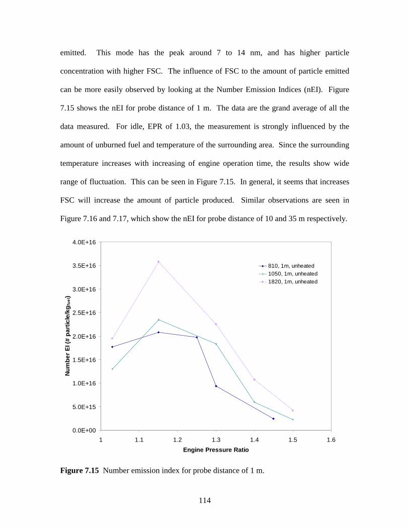
114

emitted. This mode has the peak around 7 to 14 nm, and has higher particle

concentration with higher FSC. The influence of FSC to the amount of particle emitted

can be more easily observed by looking at the Number Emission Indices (nEI). Figure

7.15 shows the nEI for probe distance of 1 m. The data are the grand average of all the

data measured. For idle, EPR of 1.03, the measurement is strongly influenced by the

amount of unburned fuel and temperature of the surrounding area. Since the surrounding

temperature increases with increasing of engine operation time, the results show wide

range of fluctuation. This can be seen in Figure 7.15. In general, it seems that increases

FSC will increase the amount of particle produced. Similar observations are seen in

Figure 7.16 and 7.17, which show the nEI for probe distance of 10 and 35 m respectively.

0.0E+00

5.0E+15

1.0E+16

1.5E+16

2.0E+16

2.5E+16

3.0E+16

3.5E+16

4.0E+16

1 1.1 1.2 1.3 1.4 1.5 1.6

Engine Pressure Ratio

Nu

mb

er E

I (#

par

ticle

/kg

fue

l)

810, 1m, unheated1050, 1m, unheated1820, 1m, unheated

Figure 7.15 Number emission index for probe distance of 1 m.

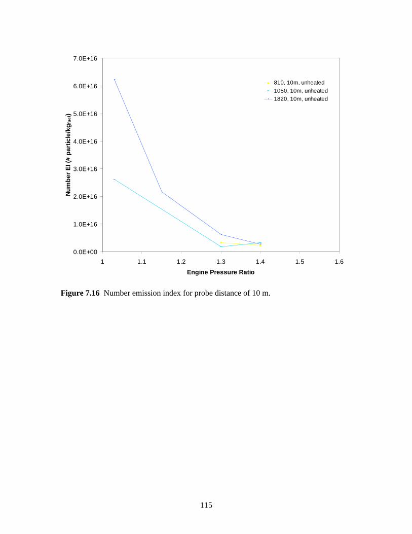
115

0.0E+00

1.0E+16

2.0E+16

3.0E+16

4.0E+16

5.0E+16

6.0E+16

7.0E+16

1 1.1 1.2 1.3 1.4 1.5 1.6

Engine Pressure Ratio

Nu

mb

er E

I (#

par

ticle

/kg

fue

l)

810, 10m, unheated1050, 10m, unheated1820, 10m, unheated

Figure 7.16 Number emission index for probe distance of 10 m.

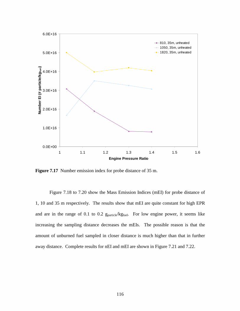
116

0.0E+00

1.0E+16

2.0E+16

3.0E+16

4.0E+16

5.0E+16

6.0E+16

1 1.1 1.2 1.3 1.4 1.5 1.6

Engine Pressure Ratio

Nu

mb

er E

I (#

par

ticle

/kg

fue

l)810, 35m, unheated1050, 35m, unheated1820, 35m, unheated

Figure 7.17 Number emission index for probe distance of 35 m.

Figure 7.18 to 7.20 show the Mass Emission Indices (mEI) for probe distance of

1, 10 and 35 m respectively. The results show that mEI are quite constant for high EPR

and are in the range of 0.1 to 0.2 gparticle/kgfuel. For low engine power, it seems like

increasing the sampling distance decreases the mEIs. The possible reason is that the

amount of unburned fuel sampled in closer distance is much higher than that in further

away distance. Complete results for nEI and mEI are shown in Figure 7.21 and 7.22.

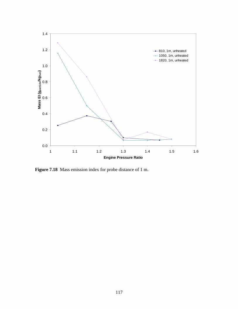
117

0.0

0.2

0.4

0.6

0.8

1.0

1.2

1.4

1 1.1 1.2 1.3 1.4 1.5 1.6

Engine Pressure Ratio

Mas

s E

I (g

par

ticl

e/k

gfu

el)

810, 1m, unheated1050, 1m, unheated1820, 1m, unheated

Figure 7.18 Mass emission index for probe distance of 1 m.

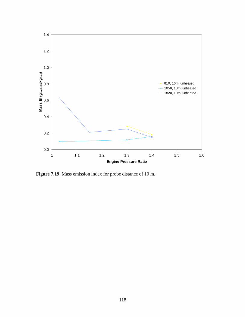
118

0.0

0.2

0.4

0.6

0.8

1.0

1.2

1.4

1 1.1 1.2 1.3 1.4 1.5 1.6

Engine Pressure Ratio

Mas

s E

I (g

par

ticl

e/k

gfu

el)

810, 10m, unheated1050, 10m, unheated1820, 10m, unheated

Figure 7.19 Mass emission index for probe distance of 10 m.

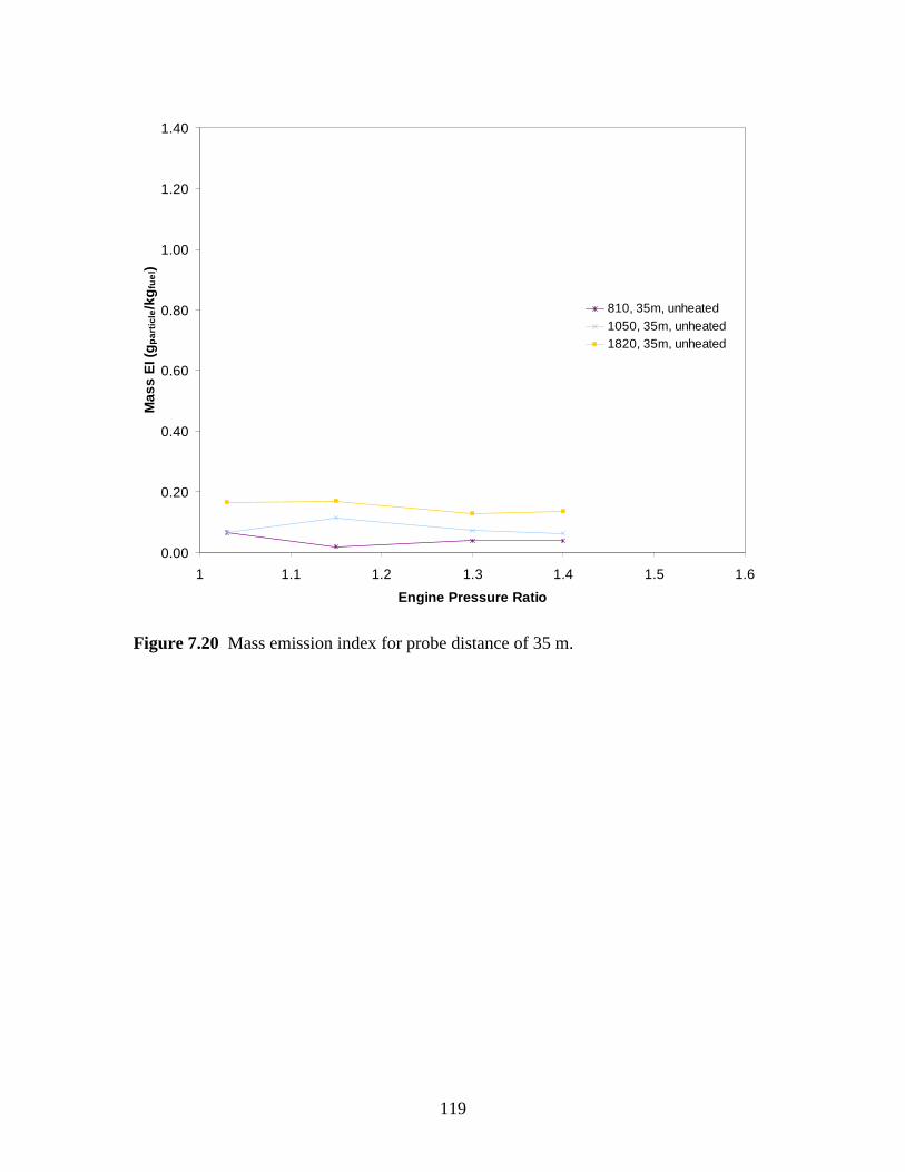
119

0.00

0.20

0.40

0.60

0.80

1.00

1.20

1.40

1 1.1 1.2 1.3 1.4 1.5 1.6

Engine Pressure Ratio

Mas

s E

I (g

par

ticl

e/k

gfu

el)

810, 35m, unheated1050, 35m, unheated1820, 35m, unheated

Figure 7.20 Mass emission index for probe distance of 35 m.

120

0.0E+00

1.0E+16

2.0E+16

3.0E+16

4.0E+16

5.0E+16

6.0E+16

7.0E+16

8.0E+16

1 1.1 1.2 1.3 1.4 1.5 1.6

Engine Pressure Ratio

Nu

mb

er E

I (#

par

ticle

/kg

fue

l)810, 1m, unheated810, 1m, heated810, 10m, unheated810, 10m, heated810, 35m, unheated810, 35m, heated1050, 1m, unheated1050, 1m, heated1050, 10m, unheated1050, 10m, heated1050, 25m, unheated1050, 25m, heated1050, 35m, unheated1050, 35m, heated1820, 1m, unheated1820, 1m, heated1820, 10m, unheated1820, 10m, heated1820, 25m, unheated1820, 25m, heated1820, 35m, unheated1820, 35m, heated

Figure 7.21 Number emission index for Boeing 757 engine.

121

0.0

0.2

0.4

0.6

0.8

1.0

1.2

1.4

1 1.1 1.2 1.3 1.4 1.5 1.6

Engine Pressure Ratio

Mas

s E

I (g

par

ticl

e/k

gfu

el)

810, 1m, unheated810, 1m, heated810, 10m, unheated810, 10m, heated810, 35m, unheated810, 35m, heated1050, 1m, unheated1050, 1m, heated1050, 10m, unheated1050, 10m, heated1050, 25m, unheated1050, 25m, heated1050, 35m, unheated1050, 35m, heated1820, 1m, unheated1820, 1m, heated1820, 10m, unheated1820, 10m, heated1820, 25m, unheated1820, 25m, heated1820, 35m, unheated1820, 35m, heated

Figure 7.22 Mass emission index for Boeing 757 engine.

122

7.4 References

1. Anderson, B. E., Cofer, W. R., Bagwell, D. R., Barrick, J. W., Hudgins, C. H., and Brunke, K. E. (1998). Airborne Observations of Aircraft Aerosol Emissions, 1: Total and Nonvolatile Particle Emission Indices. Geophysical Research Letter. 25:1689-1692. 2. Anderson, B. E., Cofer, W. R., Barrick, J. W., Bagwell, D. R., and Hudgins, C. H. (1998). Airborne Observation of Aircraft Aerosol Emissions, 2: Factors Controlling Volatile Particle Production. Geophysical Research Letter. 25:1693-1696. 3. Chen, D., and Pui, D. Y. H. (1997). Numerical Modeling of the Performance of Differential Mobility Analyzers for Nanometer Aerosol Measurements. Journal of Aerosol Science. 28:985-1004. 4. Chen, D., and Pui, D. Y. H. (1999). A High Efficiency, High Throughput Unipolar Aerosol Charger for Nanoparticles. Journal of Nanoparticle Research. 1:115-126. 5. Chen, D., Pui, D. Y. H., Hummes, D., Fissan, H., Quant, F. R., and Sem, G. J. (1998). Design and Evaluation of A Nanometer Aerosol Differential Mobility Analyzer (Nano-DMA). Journal of Aerosol Science. 29:497-509. 6. Crump, J. G., and Seinfeld, J. H. (1982). Further Results on Inversion of Aerosol Size Distribution Data: Higher-Order Sobolev Spaces and Constraints. Aerosol Science and Technology. 1:363-369. 7. Crump, J. G., and Seinfeld, J. H. (1982). A New Algorithm for Inversion of Aerosol Size Distribution Data. Aerosol Science and Technology. 1:15-34. 8. Han, H.-S., Chen, D.-R., and Pui, D. Y. H. (2002). Numerical Evaluation of Stability and Accuracy of Data Inversion Algorithms. In preparation. 9. Han, H.-S., Chen, D.-R., Pui, D. Y. H., and Anderson, B. E. (2000). A Nanometer Aerosol Size Analyzer (nASA) for Rapid Measurement of High-Concentration Size Distributions. Journal of Nanoparticle Research. 2:43-52. 10. Miake-Lye, R. C., Anderson, B. E., Cofer, W. R., Wallio, H. A., Nowicki, G. D., Ballenthin, J. O., Hunton, D. E., Knighton, W. B., Miller, T. M., Seeley, J. V., and Viggiano, A. A. (1998). SOx Oxidation and Volatile Aerosol in Aircraft Exhaust Plumes Depend on Fuel Sulfur Content. Giophysical Research Letters. 25:1677-1680. 11. Schroder, F. P., Karcher, B., Petzold, A., Baumann, R., Busen, R., Hoell, C., and Schumann, U. (1998). Ultrafine Aerosol Particles in Aircraft Plumes: In Situ Observations. Geophysical Research Letter. 25:2789-2792.

123

12. Stolzenburg, M. R. 1988. An Ultrafine Aerosol Size Distribution Measuring System. In Mechanical Engineering. University of Minnesota, Minneapolis. 13. Wolfenbarger, J. K., and Seinfeld, J. H. (1990). Inversion of Aerosol Size Distribution Data. Journal of Aerosol Science. 21:227-247. 14. Wolfenbarger, J. K., and Seinfeld, J. H. (1991). Estimating the Variance in Solution to the Aerosol Data Inversion Problem. Aerosol Science and Technology. 14:348-357.

124

APPENDIX F: Real Time Characterization of Aircraft Particulate Emission

by an Aerosol Mass Spectrometer During EXCAVATE 2002

1H. Boudries, 1M. Canagaratna, 1T. Onasch, 1D. Worsnop, , 1J. Wormhoudt,

1R. Miake-Lye 2B. Anderson

1Aerodyne Research Inc., 45 Manning Road, Billerica, MA, USA

2NASA, Hampton, VA.

1. Introduction

In this report, preliminary results from ground-based measurements carried out as part of

EXCAVATE (EXperiment to Characterize Aircraft Volatile Aerosol and Trace species Emissions)

field campaign at NASA Langley Research Center (Hampton, Virginia, USA), of exhaust aerosols

emitted by a Boeing 757 Rolls-Royce turbo engine are presented. During these measurements

the aerosol chemical composition and size distribution for different engine thrust levels, sulfur fuel

content, and different sampling distances behind the engine were characterized in real time by an

aerosol mass spectrometer.

2. Sampling and Analysis

A series of experimental tests were conducted during EXCAVATE experiment to characterize the

particle chemical composition and size distribution of major chemical components present in the

exhaust of a Boeing 757. Figure 1 summarizes the condition of engine thrust, sulphate fuel

composition and sampling distance behind the jet engine. Exhausts from three different fuels

were tested (low sulfate fuel 810 PPM, intermediate 1050 ppm, and high 1820 ppm) at 5-engine

thrust levels measured in engine pressure ratio (EPR), 1.03 (Idle), 1.15, 1.3, 1.4 and 1.5 EPR.

Four different sampling distances (1, 10, 25 and 35 meters) behind the jet engine were used

during this experiment. The exhaust aerosols PM2.5 emitted by the Rolls-Royce engine were

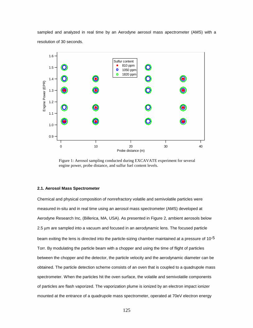
125

sampled and analyzed in real time by an Aerodyne aerosol mass apectrometer (AMS) with a

resolution of 30 seconds.

2.1. Aerosol Mass Spectrometer

Chemical and physical composition of nonrefractory volatile and semivolatile particles were

measured in-situ and in real time using an aerosol mass spectrometer (AMS) developed at

Aerodyne Research Inc, (Billerica, MA, USA). As presented in Figure 2, ambient aerosols below

2.5 µm are sampled into a vacuum and focused in an aerodynamic lens. The focused particle

beam exiting the lens is directed into the particle-sizing chamber maintained at a pressure of 10-5

Torr. By modulating the particle beam with a chopper and using the time of flight of particles

between the chopper and the detector, the particle velocity and the aerodynamic diameter can be

obtained. The particle detection scheme consists of an oven that is coupled to a quadrupole mass

spectrometer. When the particles hit the oven surface, the volatile and semivolatile components

of particles are flash vaporized. The vaporization plume is ionized by an electron impact ionizer

mounted at the entrance of a quadrupole mass spectrometer, operated at 70eV electron energy

Figure 1: Aerosol sampling conducted during EXCAVATE experiment for several engine power, probe distance, and sulfur fuel content levels.

1.6

1.5

1.4

1.3

1.2

1.1

1.0

0.9

Eng

ine

Pow

er (

EP

R)

403020100Probe distance (m)

Sulfur content 810 ppm 1050 ppm 1820 ppm

126

and scanned in a range of 1-300 atomic mass units. Detailed information about the AMS is well

documented in Jayne et al. (2000) and the data analysis (Jimenez et al., 2003).

Quantitative mass calibration of the instrument was performed by using a pure

ammonium nitrate aerosol source. Particles were generated with an atomizer (TSI, Model 3076,

USA) and then dried by passing the airflow through a silica gel. The monodisperse aerosol was

generated by passing the polydisperse flow exiting the dryer into a differential mobility analyzer

(TSI, Model DMA 3071). Detailed information about quantitative mass loading and size-

distribution calibration is presented in Jayne et al. (2000).

QuadrupoleMass Spectrometer

Thermal Vaporization

&Electron Impact

Ionization

Aerodynamic Lens

(2 Torr)

Chopper

Turbo Pump

Turbo Pump

Turbo Pump

TOF Region

Particle Beam Generation

Aerodynamic Sizing Particle Composition

QuadrupoleMass Spectrometer

Thermal Vaporization

&Electron Impact

Ionization

Aerodynamic Lens

(2 Torr)

Chopper

Turbo Pump

Turbo Pump

Turbo Pump

TOF Region

Particle Beam Generation

Aerodynamic Sizing Particle Composition

Figure 2: Aerosol nass spectrometer (AMS) used for chemical and physical composition of submicron aerosol.

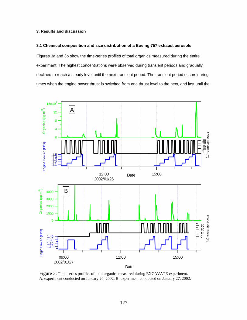
127

3. Results and discussion

3.1 Chemical composition and size distribution of a Boeing 757 exhaust aerosols

Figures 3a and 3b show the time-series profiles of total organics measured during the entire

experiment. The highest concentrations were observed during transient periods and gradually

declined to reach a steady level until the next transient period. The transient period occurs during

times when the engine power thrust is switched from one thrust level to the next, and last until the

16x103

12

8

4

0

Org

anic

s (µ

g m

-3)

12:002002/01/26

15:00Date

1.51.41.31.21.1

Engi

ne P

ower

(EP

R) 25

2015105

Probe Distance (m

)

A

Figure 3: Time-series profiles of total organics measured during EXCAVATE experiment. A: experiment conducted on January 26, 2002. B: experiment conducted on January 27, 2002.

4000

3000

2000

1000

0

Org

anic

s (µ

g m

-3)

09:002002/01/27

12:00 15:00

Date

1.401.301.201.10

Engi

n Po

wer

(EP

R)

3020100

Probe distance (m)

B

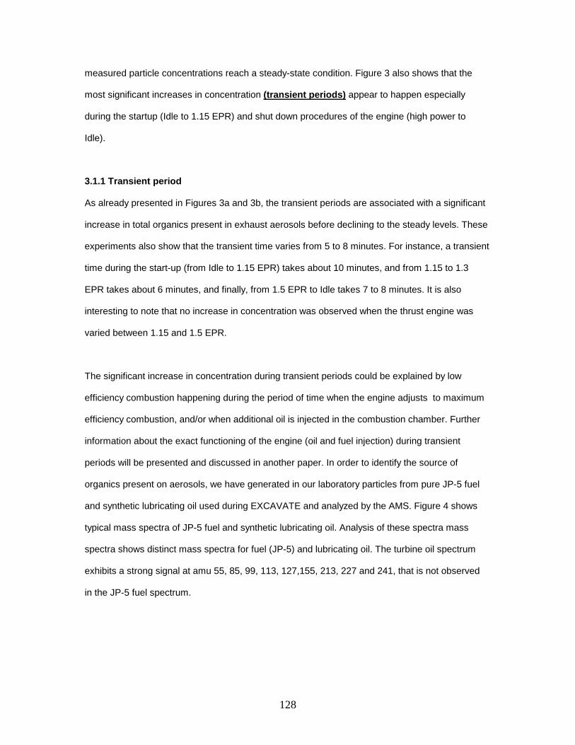
128

measured particle concentrations reach a steady-state condition. Figure 3 also shows that the

most significant increases in concentration (transient periods) appear to happen especially

during the startup (Idle to 1.15 EPR) and shut down procedures of the engine (high power to

Idle).

3.1.1 Transient period

As already presented in Figures 3a and 3b, the transient periods are associated with a significant

increase in total organics present in exhaust aerosols before declining to the steady levels. These

experiments also show that the transient time varies from 5 to 8 minutes. For instance, a transient

time during the start-up (from Idle to 1.15 EPR) takes about 10 minutes, and from 1.15 to 1.3

EPR takes about 6 minutes, and finally, from 1.5 EPR to Idle takes 7 to 8 minutes. It is also

interesting to note that no increase in concentration was observed when the thrust engine was

varied between 1.15 and 1.5 EPR.

The significant increase in concentration during transient periods could be explained by low

efficiency combustion happening during the period of time when the engine adjusts to maximum

efficiency combustion, and/or when additional oil is injected in the combustion chamber. Further

information about the exact functioning of the engine (oil and fuel injection) during transient

periods will be presented and discussed in another paper. In order to identify the source of

organics present on aerosols, we have generated in our laboratory particles from pure JP-5 fuel

and synthetic lubricating oil used during EXCAVATE and analyzed by the AMS. Figure 4 shows

typical mass spectra of JP-5 fuel and synthetic lubricating oil. Analysis of these spectra mass

spectra shows distinct mass spectra for fuel (JP-5) and lubricating oil. The turbine oil spectrum

exhibits a strong signal at amu 55, 85, 99, 113, 127,155, 213, 227 and 241, that is not observed

in the JP-5 fuel spectrum.

129

Figure 4: Typical mass spectra of JP5 and lubricating oil used during EXCAVATE field experiment.

100

101

102

103

104

Nitr

ate

Equi

vale

nt M

ass

Con

cent

ratio

n (µ

g m

-3)

2802402001601208040

Lubricating Oil8599

113

155

127

0.1

1

10

100

1000

Nitr

ate

Equi

vale

nt M

ass

Con

cent

ratio

n (µ

g m

-3)

2802402001601208040m/z (daltons)

JP5

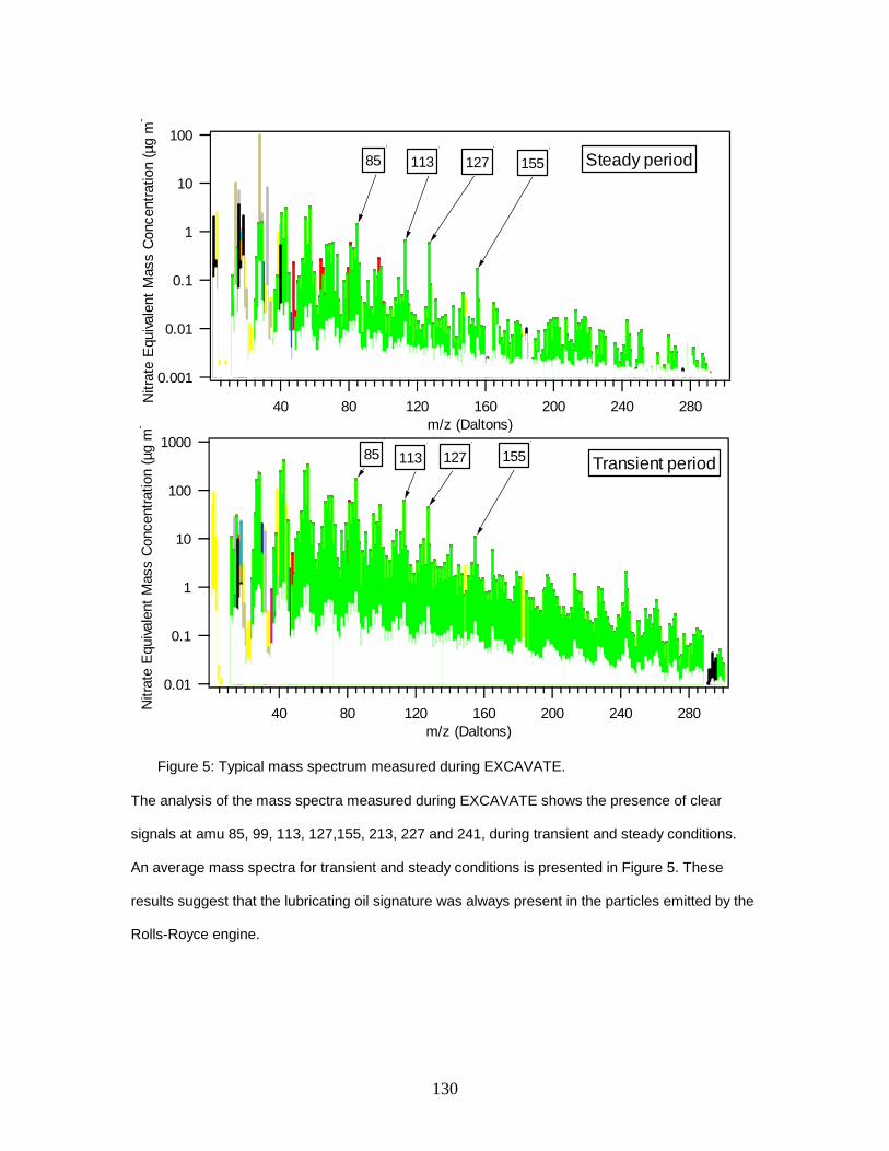
130

The analysis of the mass spectra measured during EXCAVATE shows the presence of clear

signals at amu 85, 99, 113, 127,155, 213, 227 and 241, during transient and steady conditions.

An average mass spectra for transient and steady conditions is presented in Figure 5. These

results suggest that the lubricating oil signature was always present in the particles emitted by the

Rolls-Royce engine.

Figure 5: Typical mass spectrum measured during EXCAVATE.

0.001

0.01

0.1

1

10

100N

itrat

e E

quiv

alen

t M

ass

Con

cent

ratio

n (µ

g m

-3

2802402001601208040m/z (Daltons)

Steady period85 113 127 155

0.01

0.1

1

10

100

1000

Nitr

ate

Equ

ival

ent

Mas

s C

once

ntra

tion

(µg

m-3

2802402001601208040m/z (Daltons)

Transient period85 113 127 155

131

If we assume that the Rolls-Royce engine operates at different conditions (combustion

efficiency, fuel and oil injection, etc.) we would expect to see a difference in aerosol composition

between transient and steady conditions. In order to evaluate the variation in aerosol composition

between transient and nontransient periods, variation of oil signature, plotted as function of total

organics measured during the entire experiment (January 27, 2002), will be used. In this case,

the oil signature is estimated as a total signal from amu 85, 99, 113, 127, 155, 213, 227, and

241. As shown in Figure 6, the oil-to-organic ratios show quite identical experimental slopes

measured during transient and steady conditions equal to 0.438 (R2= 0.86) and 0.451 (R2=0.98),

respectively. Only a slight difference of 2.8 percent in the experimental slope is observed,

suggesting no significant variation in aerosol composition between transient and steady condition

Figure 6: Variation of oil signature versus total organic during transient and steady conditions.

0.001

0.01

0.1

1

10

100

1000

Oil

sign

atur

e

0.1 1 10 100 1000Organics (µg m

-3)

<--------Transient--------->

<-------Steady conditions-------->

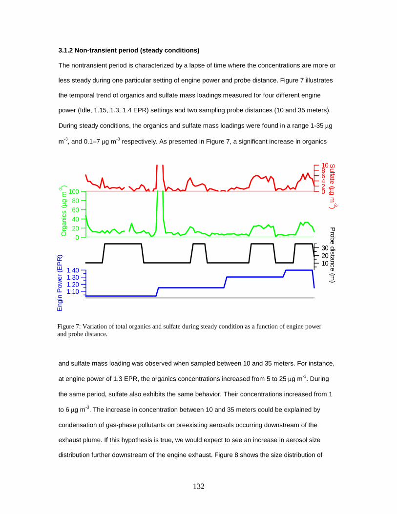
132

3.1.2 Non-transient period (steady conditions)

The nontransient period is characterized by a lapse of time where the concentrations are more or

less steady during one particular setting of engine power and probe distance. Figure 7 illustrates

the temporal trend of organics and sulfate mass loadings measured for four different engine

power (Idle, 1.15, 1.3, 1.4 EPR) settings and two sampling probe distances (10 and 35 meters).

During steady conditions, the organics and sulfate mass loadings were found in a range 1-35 µg

m-3, and 0.1–7 µg m-3 respectively. As presented in Figure 7, a significant increase in organics

and sulfate mass loading was observed when sampled between 10 and 35 meters. For instance,

at engine power of 1.3 EPR, the organics concentrations increased from 5 to 25 µg m-3. During

the same period, sulfate also exhibits the same behavior. Their concentrations increased from 1

to 6 µg m-3. The increase in concentration between 10 and 35 meters could be explained by

condensation of gas-phase pollutants on preexisting aerosols occurring downstream of the

exhaust plume. If this hypothesis is true, we would expect to see an increase in aerosol size

distribution further downstream of the engine exhaust. Figure 8 shows the size distribution of

100806040200O

rgan

ics

(µg

m-3

)

dat

1086420

Sulfate (µg m

-3)

1.401.301.201.10

Eng

in P

ower

(E

PR

)

302010

Probe distance (m

)

Figure 7: Variation of total organics and sulfate during steady condition as a function of engine power and probe distance.

133

organics and sulfate as a function of probe distance (measured at 1, 10, 25, and 35 M) and at

engine power of 1.4 EPR. This figure shows that the size distribution shift to larger sizes when

sampled further downstream of the engine exhaust. This shift in size distribution confirms the

presence of particle growth. Organics and sulfate seem to have similar aerodynamic diameters of

about 30 nm when measured at 1 m behind the engine and increase when measured further

downstream of the engine exhaust. The increase in the aerodynamic diameter of organic

aerosols is found to be more pronounced than that of sulfate particles. For organics, the

aerodynamic diameters increase from 30 to 300 nm, and from 30 to 70 nm for sulfate. The

different growth behavior at the sulfate and organic containing particles suggests that they are

externally mixed.

600

400

200

0

102 3 4 5 6 7 8 9

1002 3 4 5 6 7 8 9

1000Aerodynamic Diameter (nm)

60

40

20

0

Sulphate µg m

-3

35m4000

3000

2000

1000

0

Org

anic

s µg

m-3

102 3 4 5 6 7 8 9

1002 3 4 5 6 7 8 9

1000

300

250

200

150

100

50

0

25m

600

400

200

0

Org

anic

s µg

m-3

102 3 4 5 6 7 8 9

1002 3 4 5 6 7 8 9

1000

300

250

200

150

100

50

0

1m 500

400

300

200

100

0

102 3 4 5 6 7 8 9

1002 3 4 5 6 7 8 9

1000

50

40

30

20

10

0

Sulphate µg m

-3

10 m

600

400

200

0

102 3 4 5 6 7 8 9

1002 3 4 5 6 7 8 9

1000Aerodynamic Diameter (nm)

60

40

20

0

Sulphate µg m

-3

35m4000

3000

2000

1000

0

Org

anic

s µg

m-3

102 3 4 5 6 7 8 9

1002 3 4 5 6 7 8 9

1000

300

250

200

150

100

50

0

25m

600

400

200

0

Org

anic

s µg

m-3

102 3 4 5 6 7 8 9

1002 3 4 5 6 7 8 9

1000

300

250

200

150

100

50

0

1m 500

400

300

200

100

0

102 3 4 5 6 7 8 9

1002 3 4 5 6 7 8 9

1000

50

40

30

20

10

0

Sulphate µg m

-3

10 m

Figure 8: Variation of aerodynamic diameter of sulfate (red) and organics (green) as a function of probe distance and measured for engine power of 1.4 EPR.

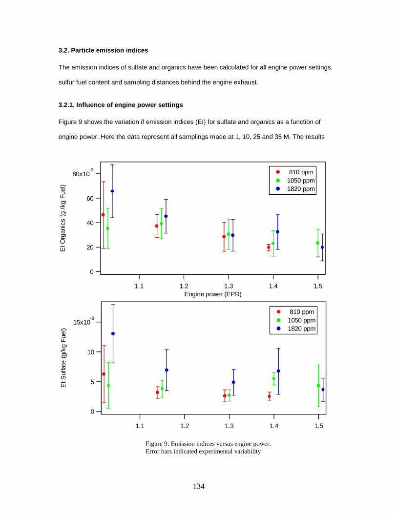
134

3.2. Particle emission indices

The emission indices of sulfate and organics have been calculated for all engine power settings,

sulfur fuel content and sampling distances behind the engine exhaust.

3.2.1. Influence of engine power settings

Figure 9 shows the variation if emission indices (EI) for sulfate and organics as a function of

engine power. Here the data represent all samplings made at 1, 10, 25 and 35 M. The results

15x10-3

10

5

0

EI S

ulfa

te (

g/kg

Fue

l)

1.51.41.31.21.1

810 ppm 1050 ppm 1820 ppm

80x10-3

60

40

20

0

EI O

rgan

ics

(g /

kg F

uel)

1.51.41.31.21.1Engine power (EPR)

810 ppm 1050 ppm 1820 ppm

Figure 9: Emission indices versus engine power. Error bars indicated experimental variability

135

show that the EI of organics decrease with engine power. At high engine power (1.5 EPR), the

organic EI is estimated to 20-25 µg kg-1 of fuel, while at idle (1.03 EPR) the average EI is about

50 µg kg-1 of fuel. The decrease in EI as a function of engine power could be explained by better

efficiency combustion at high engine power, and consequently, a reduction in the emissions of

unburned fuel and oil. It is also important to note that the EI of organics as a function of engine

power is found to be independent of fuel sulfur content.

Except for measurements made at idle (1.03 EPR), emission indices of sulfate appear to be

independent of engine power settings and proportional to the fuel sulfur content. The highest EI

correspond to the highest sulfur fuel content. For fuel sulfur content of 810 ppm, 1050 ppm and

1820 ppm, the average EI of sulfate are found equal to 2.5, 4 and 6 g kg-1 of fuel, respectively.

The highest EI measured at idle could be due to quantification errors for sulfate from interference

from organics. It is also possible that the steady-state was not really reached, and the high level

reflects data measured from transient period.

3.2.2. Influence of sampling distance

Figure 10 shows the variation of EI as a function of sampling probe distance measured for all

sulfur fuel content. Here the EI are found positively correlated with probe distance. The lowest EI

are measured at 1 M behind the engine and the highest EI are measured at 35 M behind the

engine. For all fuel used, the sulfate EIs increase with distance suggesting aerosol sulfate growth

through gas to particle conversion downstream of the exhaust plumes. This conversion is

occurring as the exhaust cool down as a consequence of dilution with ambient air. This is

confirmed in Figure 8, where the size distribution of sulfate shift to bigger sizes when sampled

downstream of the engine exhaust.

For sulfate, the EI are also found to be a function of sulfur fuel content. The lowest EI are

measured for the lowest fuel sulfur content and vice-versa. At 35 M behind the engine, the sulfate

EI increase by a factor of 2.89, while the fuel sulfur content increased by 2.14. Figure 11 shows

the normalized Eis to 810 ppm of FSC as a function of probe distance. As presented in Figure 11,

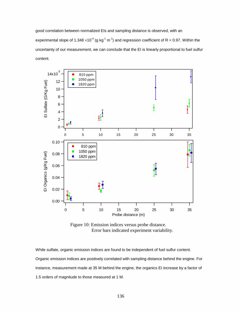
136

good correlation between normalized EIs and sampling distance is observed, with an

experimental slope of 1.348 ×10-4 (g kg-1 m-1) and regression coefficient of R = 0.97. Within the

uncertainty of our measurement, we can conclude that the EI is linearly proportional to fuel sulfur

content.

While sulfate, organic emission indices are found to be independent of fuel sulfur content.

Organic emission indices are positively correlated with sampling distance behind the engine. For

instance, measurement made at 35 M behind the engine, the organics EI increase by a factor of

1.5 orders of magnitude to those measured at 1 M.

14x10-3

12

10

8

6

4

2

0

EI S

ulfa

te (

G/K

g F

uel)

35302520151050

810 ppm 1050 ppm 1820 ppm

0.10

0.08

0.06

0.04

0.02

0.00

EI O

rgan

ics

(g/K

g F

uel)

35302520151050Probe distance (m)

810 ppm 1050 ppm 1820 ppm

Figure 10: Emission indices versus probe distance. Error bars indicated experiment variability.

137

Conclusion

During EXCAVATE experiment, particulate emissions from a Boeing 757 equipped with a Rolls

Royce engine were studied. Chemical and physical composition of PM2.5 was measured in real

time with a resolution of 30 seconds. Time series profile of total organics and sulfate shows a

presence of a transient period associated with extremely high mass loadings of pollutants. Thus,

the transient period appears to happen during the start-up of the engine, from idle (1.03 EPR) to

1.15 EPR, and during engine shut down (1.5 to idle). Up to 5000 µg m-3 of organic was measured

during transient period, whereas concentration during steady conditions was in a range of 1 to 30

µg m-3. The presence of lubricating oil was found during steady and transient periods. Sulfate

emission indices were found dependent on sulfur fuel content and positively correlated to the

sampling probe distance. Organics emissions are also found positively correlated with sampling

Figure 11: Emission indices normalized to 810 ppm of sulfur fuel content versus probe distance.

0.10

5x10-3

4

3

2

1

No

rma

lize

d s

ulfa

te E

I (g

/Kg

Fu

el)

3530252015105Probe distance (m)

R=0.98EI=0.0001348 x [dis tance] + 0.00053328

138

distance but independent of sulfur fuel content. For EPR higher than 1.15, the EI are found more

or less independent of the Engine power.

References

Brown R.C., Miake-Lye, R.C., Anderson, M.R. and Kolb, C.E, 1997: Aircraft sulfur emissions and the formation of visible contrails. Geophysical Research Letters, 24, pp. 385-388. Curtius J., Arnold, F., Schulte, P, 2002: Sulfuric acid measurements in the exhaust plume of a jet aircraft in flight: Implication for the sulfuric acid formation efficiency. Geophysical Research Letters, 29, No.7, p. 10129. Hagen D.E., Whitefield, P.D., 1996: . Particulate emissions in the exhaust plume from commercial jet aircraft under cruise conditions. Journal of Geophysical Research, 101, D14, pp. 19551-19557. Jayne Jensen E.J.,Toon, O.B., 1997: The potential impact of soot particles from aircraft exhaust on cirrus clouds. Geophysical Research Letters, 24, pp. 249-252. Jimenez J. L., Jayne, J.T., Shi, Q., Kolb, C.E., Worsnop, D.R., Yourshaw, I., Seinfeld, J.H., Flagan, R.C., Zhang, X., Smith, K.A., Morris, J.W., Davidovits, P., 2003 : Ambient aerosol sampling using the Aerodyne Aerosol Mass Spectrometer. Journal of Geophysical Research 108, D7. Miake-Lye R.C., Anderson, B.E., Cofer, W.R., Wallio, H.A., Norwicki, G.D., Ballenthin, J.O., Hunton, D.E., Knighton, W.B., Miller, T.M., Seeley, J.V., Viggiano, A.A., 1998: SOx oxidation and volatile aerosol in aircraft exhaust plumes depend on fuel sulfur content. Geophysical Research Letters, 25, No.10, pp.1677-1680.

139

APPENDIX G: AFRL Report on the NASA EXCAVATE Project

Thomas M. Miller, John O. Ballenthin, and Albert A. Viggiano

Air Force Research Laboratory, Space Vehicles Directorate,

29 Randolph Road, Hanscom AFB, MA 01731-3010 Introduction The NASA EXCAVATE Project (Experiment to Characterize Aircraft Volatile Aerosol and Trace Species Emissions) took place in January of 2002 at NASA-Langley Research Center. The purpose was to analyze aerosol, gas and ion emissions from the jet engines of NASA Boeing-757 and T-38 aircraft operating with fuels of different sulfur levels, and with the Boeing 757 engine at distances of 1 and 10 m from the tip of the sampling pipe. This report concerns a subset of the measurements, those made by the Air Force Research Laboratory (AFRL) for emission indices of SO2 and the concentration and mass speciation of chemiions, under various engine conditions (power setting and fuel type). [Radical-radical reactions (including excited-state reactions) in the combustion process can result in ionization (so-called chemiions).] The AFRL Chemical Ionization Mass Spectrometer (CIMS) was used to determine the mixing ratio of SO2 in the engine exhaust. An AFRL Ion Mass Spectrometer (IMS) was used to determine the concentration and mass distribution of chemiions in the exhaust. A Gerdien condenser was used in an unsuccessful attempt to determine the chemiion concentration directly. The results of these measurements were expressed as emission indices by normalizing to NASA-Langley Research Center (LaRC) measurements of the mixing ratio of CO2 in the exhaust, above ambient levels. Figure 1 shows the experimental setup used by all instruments.

Fig. 1. The test rig bolted to the tarmac behind a

Boeing-757 engine. The IMS and CIMS instruments were mounted inside the test rig shown at the base of the sampling pipe. The Gerdien condenser was welded to the side of the sampling pipe. The tip of the sampling pipe was here 1 m behind the engine exhaust plane, and ran an additional distance of 2.29 m to the IMS inlet, or 2.51 m to the CIMS inlet. The sampling pipe had a different configuration for the T-38 aircraft, for which the engine was closer to the tarmac, and the pipe lengths were 2.22 m to the IMS inlet and 2.43 m to the CIMS inlet.

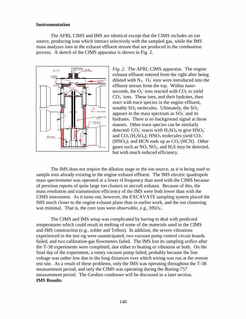
140

Instrumentation The AFRL CIMS and IMS are identical except that the CIMS includes an ion source, producing ions which interact selectively with the sampled gas, while the IMS mass analyzes ions in the exhaust effluent stream that are produced in the combustion process. A sketch of the CIMS apparatus is shown in Fig. 2.

Fig. 2. The AFRL CIMS apparatus. The engine exhaust effluent entered from the right after being diluted with N2. O3

- ions were introduced into the effluent stream from the top. Within nano-seconds, the O3

- ions reacted with CO2 to yield CO3

- ions. These ions, and their hydrates, then react with trace species in the engine effluent, notably SO2 molecules. Ultimately, the SO2 appears in the mass spectrum as SO5

- and its hydrates. There is no background signal at those masses. Other trace species can be similarly detected: CO3

- reacts with H2SO4 to give HSO4-

and CO3-(H2SO4); HNO3 molecules yield CO3

-

(HNO3); and HCN ends up as CO3-(HCN). Other

gases such as NO, NO2, and H2S may be detected, but with much reduced efficiency.

The IMS does not require the dilution stage or the ion source, as it is being used to sample ions already existing in the engine exhaust effluent. The IMS electric quadrupole mass spectrometer was operated at a lower rf frequency than used with the CIMS because of previous reports of quite large ion clusters in aircraft exhaust. Because of this, the mass resolution and transmission efficiency of the IMS were both lower than with the CIMS instrument. As it turns out, however, the EXCAVATE sampling system placed the IMS much closer to the engine exhaust plane than in earlier work, and the ion clustering was minimal. That is, the core ions were observable, e.g., HSO4

-. The CIMS and IMS setup was complicated by having to deal with predicted temperatures which could result in melting of some of the materials used in the CIMS and IMS construction (e.g., solder and Teflon). In addition, the severe vibrations experienced in the test rig were unanticipated; two vacuum pump control circuit boards failed, and two calibration-gas flowmeters failed. The IMS lost its sampling orifice after the T-38 experiments were completed, due either to heating or vibration or both. On the final day of the experiment, a rotary vacuum pump failed, probably because the line voltage was rather low due to the long distances over which wiring was run at the remote test site. As a result of these problems, only the IMS was operating throughout the T-38 measurement period, and only the CIMS was operating during the Boeing-757 measurement period. The Gerdien condenser will be discussed in a later section. IMS Results

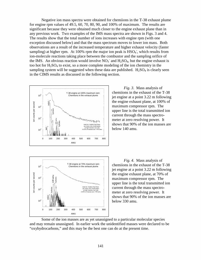
141

Negative ion mass spectra were obtained for chemiions in the T-38 exhaust plume for engine rpm values of 49.5, 60, 70, 80, 90, and 100% of maximum. The results are significant because they were obtained much closer to the engine exhaust plane than in any previous work. Two examples of the IMS mass spectra are shown in Figs. 3 and 4. The results show that the total number of ions increases with engine rpm (with one exception discussed below) and that the mass spectrum moves to lower ion mass. Both observations are a result of the increased temperature and higher exhaust velocity (faster sampling) at higher rpm. At 100% rpm the major ion peak is HSO4

-, which results from ion-molecule reactions taking place between the combustor and the sampling orifice of the IMS. An obvious reaction would involve NO3

- and H2SO4, but the engine exhaust is too hot for H2SO4 to exist, so a more complete modeling of the ion chemistry in the sampling system will be suggested when these data are published. H2SO4 is clearly seen in the CIMS results as discussed in the following section.

Fig. 3. Mass analysis of chemiions in the exhaust of the T-38 jet engine at a point 3.22 m following the engine exhaust plane, at 100% of maximum compressor rpm. The upper line is the total transmitted ion current through the mass spectro-meter at zero resolving power. It shows that 90% of the ion masses are below 140 amu.

Fig. 4. Mass analysis of chemiions in the exhaust of the T-38 jet engine at a point 3.22 m following the engine exhaust plane, at 70% of maximum compressor rpm. The upper line is the total transmitted ion current through the mass spectro-meter at zero resolving power. It shows that 90% of the ion masses are below 330 amu.

Some of the ion masses are as yet unassigned to a particular molecular species and may remain unassigned. In earlier work the unidentified masses were declared to be “oxyhydrocarbons,” and this may be the best one can do at the present time.

102

103

104

105

0 100 200 300 400 500 600 700 800

ion

coun

ts p

er s

econ

d

AMU

total ion: Implies that there are many very small peaks

at high masses, but only0.31% of masses are >745 amu

HS

O4-

NO

3-

hydr

ates

180

amu

hydr

ates

T-38 engine at 100% maximum rpm:Chemiions in the exhaust plume

102

103

104

105

0 100 200 300 400 500 600 700 800

ion

coun

ts p

er s

econ

d

AMU

total ion: Implies that there are many very small peaks

at high masses, but only2.54% of masses are >745 amu

T-38 engine at 70% maximum rpm:Chemiions in the exhaust plume

HS

O4-

hydr

ates

139

amu

hydr

ates

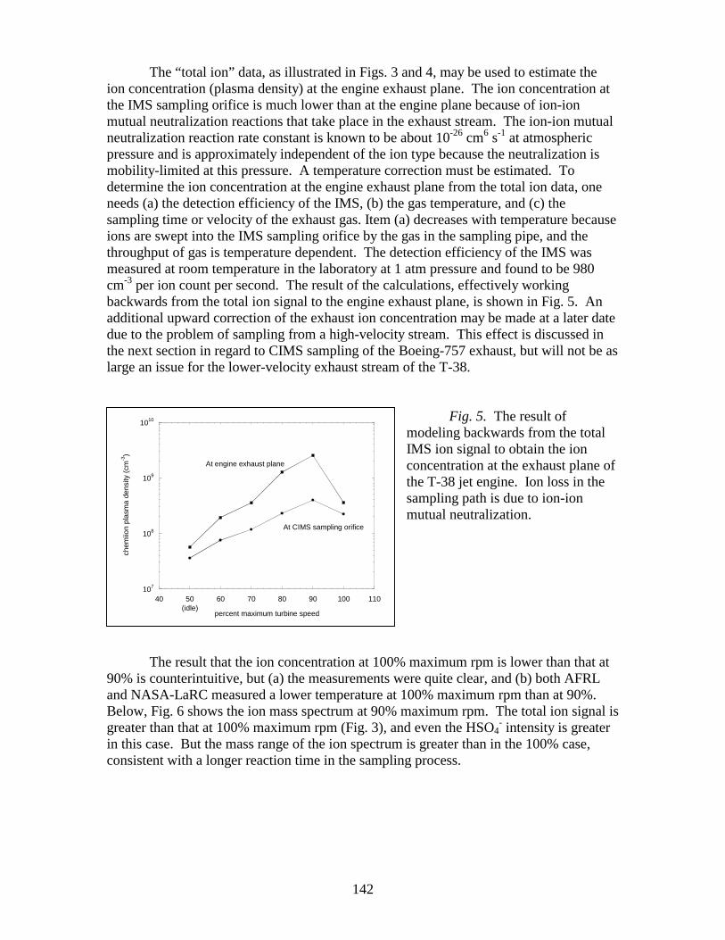
142

The “total ion” data, as illustrated in Figs. 3 and 4, may be used to estimate the ion concentration (plasma density) at the engine exhaust plane. The ion concentration at the IMS sampling orifice is much lower than at the engine plane because of ion-ion mutual neutralization reactions that take place in the exhaust stream. The ion-ion mutual neutralization reaction rate constant is known to be about 10-26 cm6 s-1 at atmospheric pressure and is approximately independent of the ion type because the neutralization is mobility-limited at this pressure. A temperature correction must be estimated. To determine the ion concentration at the engine exhaust plane from the total ion data, one needs (a) the detection efficiency of the IMS, (b) the gas temperature, and (c) the sampling time or velocity of the exhaust gas. Item (a) decreases with temperature because ions are swept into the IMS sampling orifice by the gas in the sampling pipe, and the throughput of gas is temperature dependent. The detection efficiency of the IMS was measured at room temperature in the laboratory at 1 atm pressure and found to be 980 cm-3 per ion count per second. The result of the calculations, effectively working backwards from the total ion signal to the engine exhaust plane, is shown in Fig. 5. An additional upward correction of the exhaust ion concentration may be made at a later date due to the problem of sampling from a high-velocity stream. This effect is discussed in the next section in regard to CIMS sampling of the Boeing-757 exhaust, but will not be as large an issue for the lower-velocity exhaust stream of the T-38.

Fig. 5. The result of modeling backwards from the total IMS ion signal to obtain the ion concentration at the exhaust plane of the T-38 jet engine. Ion loss in the sampling path is due to ion-ion mutual neutralization.

The result that the ion concentration at 100% maximum rpm is lower than that at

90% is counterintuitive, but (a) the measurements were quite clear, and (b) both AFRL and NASA-LaRC measured a lower temperature at 100% maximum rpm than at 90%. Below, Fig. 6 shows the ion mass spectrum at 90% maximum rpm. The total ion signal is greater than that at 100% maximum rpm (Fig. 3), and even the HSO4

- intensity is greater in this case. But the mass range of the ion spectrum is greater than in the 100% case, consistent with a longer reaction time in the sampling process.

107

108

109

1010

40 50 60 70 80 90 100 110

chem

iion

plas

ma

dens

ity (

cm-3

)

percent maximum turbine speed(idle)

At engine exhaust plane

At CIMS sampling orifice

143

Fig. 6. Mass analysis of chemiions in the exhaust of the T-38 jet engine at a point 3.22 m following the engine exhaust plane, at 90% of maximum compressor rpm. The upper line is the total transmitted ion current through the mass spectrometer at zero resolving power. It shows that 90% of the ion masses are below 290 amu.

The IMS sampling orifice fell off at the completion of the T-38 test series. It was

not possible to replace it in the field because the IMS sampling orifice plate was welded to the sampling pipe inside the test rig and not accessible in the time available. It would have been useful to examine the positive ion mass spectrum, even briefly. Earlier work at 29 m behind a jet engine showed ions at almost every mass, up to hundreds of amu, all of low intensity. The EXCAVATE test rig was so close to the engine that we could probably identify the core positive ions in a second EXCAVATE project. Furthermore, knowing now that a large mass range is not needed for the close sampling distances possible with EXCAVATE, the IMS could be set up for greater mass resolution and transmission efficiency. CIMS Results A typical CIMS spectrum is shown in Fig. 7. CO3

- ions are converted mostly to CO3

- hydrates by H2O in the exhaust stream. The hydrated ions may react more efficiently with trace gases than CO3

- itself. The appearance of SO5- and its hydrates

indicates the concentration of SO2 in the diluted effluent in the CIMS flow tube. Other species detected (NO, HCN, HNO3, and H2SO4) are indicated by labels on the respective characteristic mass peaks in Fig. 7. For the EXCAVATE data analysis, the reactant ion intensity was taken to be the sum of the CO3

- intensity and of its hydrates. Likewise, the product ion intensity was taken to be that of SO5

- and its hydrates. The background signal for the product ions was ignored, as it was only a few counts per second with the engine off.

102

103

104

105

0 100 200 300 400 500 600 700 80

ion

coun

ts p

er s

econ

d

AMU

total ion: Implies that there are many very small peaksat high masses, but only

0.89% of masses are >745 amu

T-38 engine at 90% maximum rpm:Chemiions in the exhaust plume

HS

O4-

NO

3-

hydr

ates

139

amu

177

amu

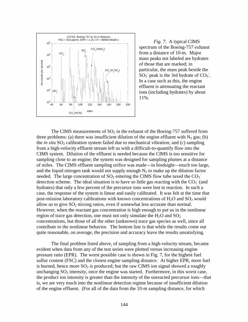
144

Fig. 7. A typical CIMS spectrum of the Boeing-757 exhaust from a distance of 10-m. Major mass peaks not labeled are hydrates of those that are marked; in particular, the mass peak beside the SO5

- peak is the 3rd hydrate of CO3-.

In a case such as this, the engine effluent is attenuating the reactant ions (including hydrates) by about 11%.

The CIMS measurements of SO2 in the exhaust of the Boeing-757 suffered from three problems: (a) there was insufficient dilution of the engine effluent with N2 gas; (b) the in situ SO2 calibration system failed due to mechanical vibration; and (c) sampling from a high-velocity effluent stream left us with a difficult-to-quantify flow into the CIMS system. Dilution of the effluent is needed because the CIMS is too sensitive for sampling close to an engine; the system was designed for sampling plumes at a distance of miles. The CIMS effluent sampling orifice was made—in hindsight—much too large, and the liquid nitrogen tank would not supply enough N2 to make up the dilution factor needed. The large concentration of SO2 entering the CIMS flow tube taxed the CO3

- detection scheme. The ideal situation is to have so little gas reacting with the CO3

- (and hydrates) that only a few percent of the precursor ions were lost to reaction. In such a case, the response of the system is linear and easily calibrated. It was felt at the time that post-mission laboratory calibrations with known concentrations of H2O and SO2 would allow us to give SO2 mixing ratios, even if somewhat less accurate than normal. However, when the reactant gas concentration is high enough to put us in the nonlinear region of trace gas detection, one must not only simulate the H2O and SO2 concentrations, but those of all the other (unknown) trace gas species as well, since all contribute to the nonlinear behavior. The bottom line is that while the results come out quite reasonable, on average, the precision and accuracy leave the results unsatisfying. The final problem listed above, of sampling from a high-velocity stream, became evident when data from any of the test series were plotted versus increasing engine pressure ratio (EPR). The worst possible case is shown in Fig. 7, for the highest fuel sulfur content (FSC) and the closest engine sampling distance. At higher EPR, more fuel is burned, hence more SO2 is produced; but the raw CIMS ion signal showed a roughly unchanging SO2 intensity, once the engine was started. Furthermore, in this worst case, the product ion intensity is greater than the intensity of the unreacted precursor ions—that is, we are very much into the nonlinear detection regime because of insufficient dilution of the engine effluent. (For all of the data from the 10-m sampling distance, for which

101

102

103

104

105

106

40 60 80 100 120 140 160 180 200

ion

coun

ts p

er s

econ

d

AMU

1/27/02, Boeing-757 at 10-m distance;FSC = 810 ppmm; EPR = 1.15; UT = 68940-69180 s

CO3

-SO

5

- CO3

-(HNO3)

NO2

-

CO3

-(HCN)

CO3

-(H2SO

4)

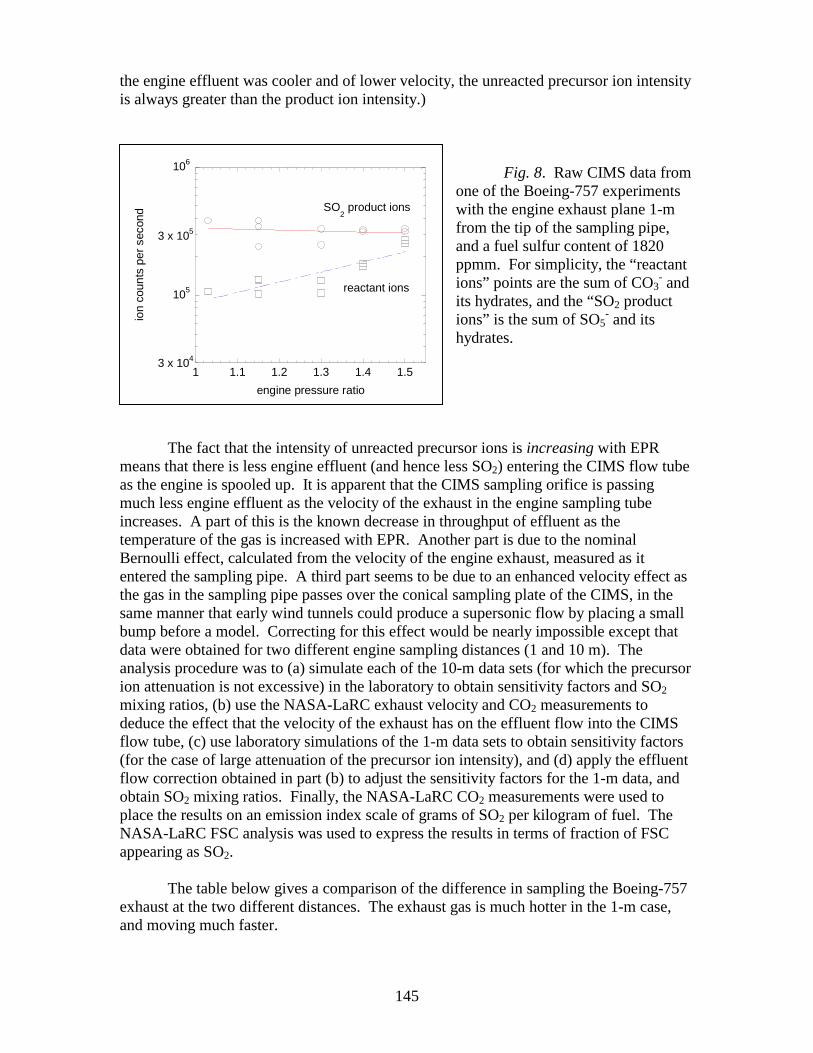
145

the engine effluent was cooler and of lower velocity, the unreacted precursor ion intensity is always greater than the product ion intensity.)

Fig. 8. Raw CIMS data from one of the Boeing-757 experiments with the engine exhaust plane 1-m from the tip of the sampling pipe, and a fuel sulfur content of 1820 ppmm. For simplicity, the “reactant ions” points are the sum of CO3

- and its hydrates, and the “SO2 product ions” is the sum of SO5

- and its hydrates.

The fact that the intensity of unreacted precursor ions is increasing with EPR means that there is less engine effluent (and hence less SO2) entering the CIMS flow tube as the engine is spooled up. It is apparent that the CIMS sampling orifice is passing much less engine effluent as the velocity of the exhaust in the engine sampling tube increases. A part of this is the known decrease in throughput of effluent as the temperature of the gas is increased with EPR. Another part is due to the nominal Bernoulli effect, calculated from the velocity of the engine exhaust, measured as it entered the sampling pipe. A third part seems to be due to an enhanced velocity effect as the gas in the sampling pipe passes over the conical sampling plate of the CIMS, in the same manner that early wind tunnels could produce a supersonic flow by placing a small bump before a model. Correcting for this effect would be nearly impossible except that data were obtained for two different engine sampling distances (1 and 10 m). The analysis procedure was to (a) simulate each of the 10-m data sets (for which the precursor ion attenuation is not excessive) in the laboratory to obtain sensitivity factors and SO2 mixing ratios, (b) use the NASA-LaRC exhaust velocity and CO2 measurements to deduce the effect that the velocity of the exhaust has on the effluent flow into the CIMS flow tube, (c) use laboratory simulations of the 1-m data sets to obtain sensitivity factors (for the case of large attenuation of the precursor ion intensity), and (d) apply the effluent flow correction obtained in part (b) to adjust the sensitivity factors for the 1-m data, and obtain SO2 mixing ratios. Finally, the NASA-LaRC CO2 measurements were used to place the results on an emission index scale of grams of SO2 per kilogram of fuel. The NASA-LaRC FSC analysis was used to express the results in terms of fraction of FSC appearing as SO2. The table below gives a comparison of the difference in sampling the Boeing-757 exhaust at the two different distances. The exhaust gas is much hotter in the 1-m case, and moving much faster.

105

106

1 1.1 1.2 1.3 1.4 1.5

ion

coun

ts p

er s

econ

d

engine pressure ratio

3 x 105

SO2 product ions

reactant ions

3 x 104

146

Table 1. NASA-LaRC data for the average Boeing-757 exhaust velocities and temperatures (T) during EXCAVATE, for the engine exhaust plane 1 or 10 m from the tip of the sampling pipe. Engine idle is EPR = 1.03; takeoff power is EPR = 1.7. EPR T T velocity velocity at 1 m at 10 m at 1 m at 10 m 1.03 580 K 329 K 73 m/s 45 m/s 1.15 615 350 187 131 1.30 640 378 275 192 1.40 660 397 319 221 1.50 686 - 351 - The formulas used in the SO2 data presentation are the same ones used in analyzing the NASA-Glenn engine test results:

(a) If all the fuel sulfur were to be converted into SO2, a fuel sulfur content (FSC) of 810 ppmm (0.081% S by mass) would give 0.00081 kg of S per kg of fuel or 0.00162 kg (1.62 g) of SO2 per kg of fuel. Thus EI(SO2) = 1.62 g/kg. The units may at times be expressed explicitly as g(SO2)/kg(fuel), or abbreviated as g/kg. A FSC of 1050 would yield EI(SO2) = 2.10 g/kg; and a FSC of 1820 would yield EI(SO2) = 3.64 g/kg.

(b) EI(SO2) = (64/12) (0.87) (SO2 ppbv/CO2 ppmv); the 0.87 is the fraction of carbon by mass, in the fuel. Dividing ppbv by ppmv puts the units of EI as g/kg, or more precisely as g(SO2)/kg(fuel). Thus, EI(SO2) = 4.64 (SO2 ppbv/CO2 ppmv).

The results are shown in Figs. 9 and 10 for the Boeing-757 at 1 and 10 m distances and are tabulated in Table 2. Points obtained on one data run in Fig. 9 (for a FSC of 1050) lie above 1, which is clearly not possible if the relevant parameters are accurate. We note that the amount of SO2 measured was similar for the two data runs for FSC = 1050, but the CO2 measurements were lower for the second set of data, leading to higher EI(SO2) and higher fraction of FSC (above 1).

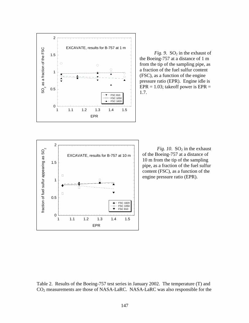
147

Fig. 9. SO2 in the exhaust of the Boeing-757 at a distance of 1 m from the tip of the sampling pipe, as a fraction of the fuel sulfur content (FSC), as a function of the engine pressure ratio (EPR). Engine idle is EPR = 1.03; takeoff power is EPR = 1.7.

Fig. 10. SO2 in the exhaust of the Boeing-757 at a distance of 10 m from the tip of the sampling pipe, as a fraction of the fuel sulfur content (FSC), as a function of the engine pressure ratio (EPR).

Table 2. Results of the Boeing-757 test series in January 2002. The temperature (T) and CO2 measurements are those of NASA-LaRC. NASA-LaRC was also responsible for the

0

0.5

1

1.5

2

1 1.1 1.2 1.3 1.4 1.5

FSC 810FSC 1050FSC 1820

SO

2 as

a fr

actio

n of

the

FS

C

EPR

EXCAVATE, results for B-757 at 1 m

0

0.5

1

1.5

2

1 1.1 1.2 1.3 1.4 1.5

FSC 1820FSC 1050FSC 810

frac

tion

of fu

el s

ulfu

r ap

pear

ing

as S

O2

EPR

EXCAVATE, results for B-757 at 10 m

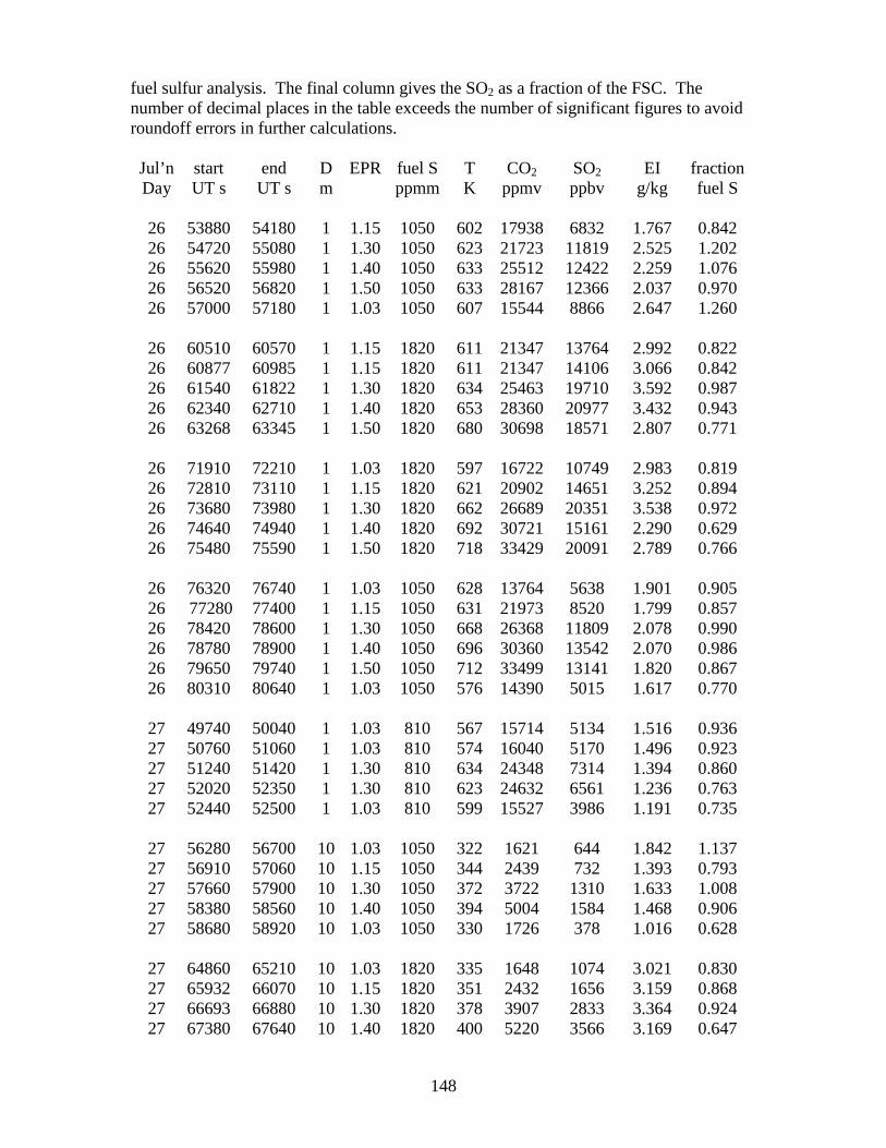
148

fuel sulfur analysis. The final column gives the SO2 as a fraction of the FSC. The number of decimal places in the table exceeds the number of significant figures to avoid roundoff errors in further calculations. Jul’n start end D EPR fuel S T CO2 SO2 EI fraction Day UT s UT s m ppmm K ppmv ppbv g/kg fuel S 26 53880 54180 1 1.15 1050 602 17938 6832 1.767 0.842 26 54720 55080 1 1.30 1050 623 21723 11819 2.525 1.202 26 55620 55980 1 1.40 1050 633 25512 12422 2.259 1.076 26 56520 56820 1 1.50 1050 633 28167 12366 2.037 0.970 26 57000 57180 1 1.03 1050 607 15544 8866 2.647 1.260 26 60510 60570 1 1.15 1820 611 21347 13764 2.992 0.822 26 60877 60985 1 1.15 1820 611 21347 14106 3.066 0.842 26 61540 61822 1 1.30 1820 634 25463 19710 3.592 0.987 26 62340 62710 1 1.40 1820 653 28360 20977 3.432 0.943 26 63268 63345 1 1.50 1820 680 30698 18571 2.807 0.771 26 71910 72210 1 1.03 1820 597 16722 10749 2.983 0.819 26 72810 73110 1 1.15 1820 621 20902 14651 3.252 0.894 26 73680 73980 1 1.30 1820 662 26689 20351 3.538 0.972 26 74640 74940 1 1.40 1820 692 30721 15161 2.290 0.629 26 75480 75590 1 1.50 1820 718 33429 20091 2.789 0.766 26 76320 76740 1 1.03 1050 628 13764 5638 1.901 0.905 26 77280 77400 1 1.15 1050 631 21973 8520 1.799 0.857 26 78420 78600 1 1.30 1050 668 26368 11809 2.078 0.990 26 78780 78900 1 1.40 1050 696 30360 13542 2.070 0.986 26 79650 79740 1 1.50 1050 712 33499 13141 1.820 0.867 26 80310 80640 1 1.03 1050 576 14390 5015 1.617 0.770 27 49740 50040 1 1.03 810 567 15714 5134 1.516 0.936 27 50760 51060 1 1.03 810 574 16040 5170 1.496 0.923 27 51240 51420 1 1.30 810 634 24348 7314 1.394 0.860 27 52020 52350 1 1.30 810 623 24632 6561 1.236 0.763 27 52440 52500 1 1.03 810 599 15527 3986 1.191 0.735 27 56280 56700 10 1.03 1050 322 1621 644 1.842 1.137 27 56910 57060 10 1.15 1050 344 2439 732 1.393 0.793 27 57660 57900 10 1.30 1050 372 3722 1310 1.633 1.008 27 58380 58560 10 1.40 1050 394 5004 1584 1.468 0.906 27 58680 58920 10 1.03 1050 330 1726 378 1.016 0.628 27 64860 65210 10 1.03 1820 335 1648 1074 3.021 0.830 27 65932 66070 10 1.15 1820 351 2432 1656 3.159 0.868 27 66693 66880 10 1.30 1820 378 3907 2833 3.364 0.924 27 67380 67640 10 1.40 1820 400 5220 3566 3.169 0.647

149

27 68020 68340 10 1.03 810 327 1599 485 1.405 0.867 27 68940 69180 10 1.15 810 359 2428 790 1.509 0.932 27 69700 69890 10 1.30 810 382 3799 1230 1.501 0.926 27 70410 70670 10 1.40 810 401 5085 1577 1.440 0.889 Gerdien Condenser The Gerdien condenser was intended to provide a direct measurement of the charge density in the engine exhaust. The Gerdien condenser had a 12-inch current collector length and 1-inch I.D. The principle of operation is to apply a voltage sufficient to sweep all ions to the central collector or to the tube walls. The ion density (assuming singly-charged ions) could then be deduced if the exhaust velocity was known (a parameter provided by NASA-LaRC). Furthermore, if the signal-to-noise ratio is high enough, one can infer information about the relative mobilities (and hence masses) of the charge carriers from changes in the collected current with applied voltage. The Gerdien condenser worked well in a laboratory setting with ions in a clean gas flow, but failed in the field. Within a few minutes of engine startup, only small currents that appeared to be leakage currents were obtained. Examination of the Gerdien condenser after the test showed it to be coated with what appeared to be baked-on oil. This observation is consistent with the diesel-oil smell of the exhaust at startup or upon any increase in power, and with measurements of unburned oil or fuel, made by the aerosol groups. Thus, we were unable to provide an independent (and potentially more accurate) measurement of the concentration of chemiions in the jet exhaust for comparison to that deduced from the IMS data, but we learned valuable lessons from this first attempt: (1) the Gerdien condenser must be protected during engine startup, and indeed should only be exposed to the exhaust during a brief measurement period—there are various ways of doing this; and (2) the wiring must be protected from the coastal Virginia dew and rain. It should also be mentioned for future reference that the Gerdien condenser must be firmly mounted because of the severe vibrations experienced during the tests; the unit became airborne during one measurement period due to an error in welding the unit to the sampling pipe.

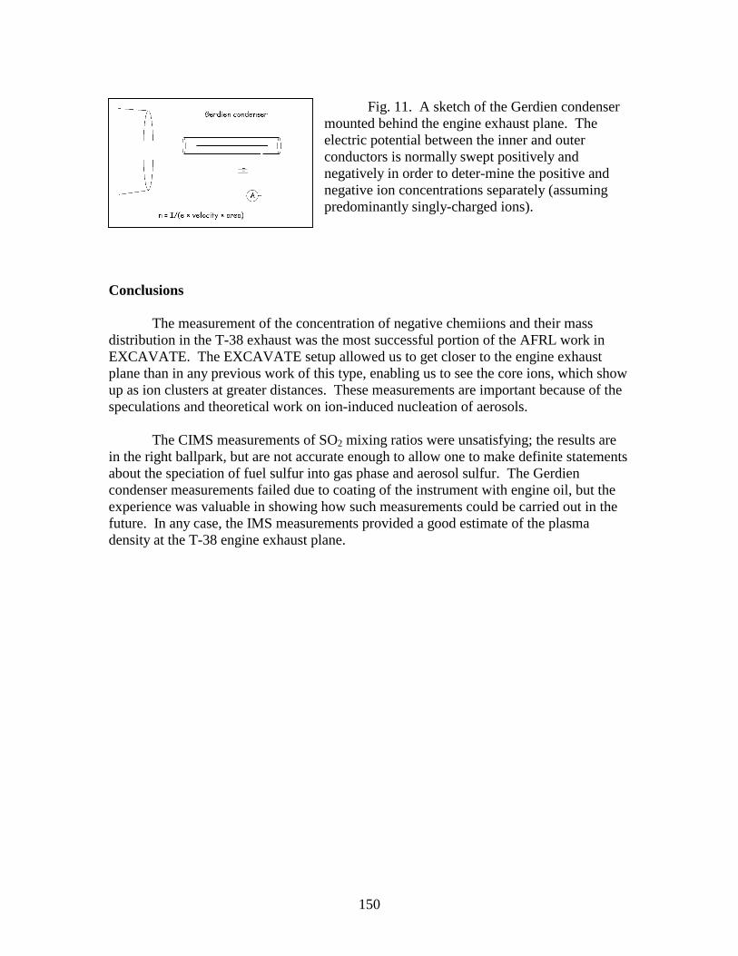
150

Fig. 11. A sketch of the Gerdien condenser mounted behind the engine exhaust plane. The electric potential between the inner and outer conductors is normally swept positively and negatively in order to deter-mine the positive and negative ion concentrations separately (assuming predominantly singly-charged ions).

Conclusions The measurement of the concentration of negative chemiions and their mass distribution in the T-38 exhaust was the most successful portion of the AFRL work in EXCAVATE. The EXCAVATE setup allowed us to get closer to the engine exhaust plane than in any previous work of this type, enabling us to see the core ions, which show up as ion clusters at greater distances. These measurements are important because of the speculations and theoretical work on ion-induced nucleation of aerosols. The CIMS measurements of SO2 mixing ratios were unsatisfying; the results are in the right ballpark, but are not accurate enough to allow one to make definite statements about the speciation of fuel sulfur into gas phase and aerosol sulfur. The Gerdien condenser measurements failed due to coating of the instrument with engine oil, but the experience was valuable in showing how such measurements could be carried out in the future. In any case, the IMS measurements provided a good estimate of the plasma density at the T-38 engine exhaust plane.

151

Appendix H: Particle Size Distributions Measured in B757 Engine Plume During EXCAVATE

Terry Sanders, Paul Penko, Steve Culler, Monica Rivera*

NASA Glenn Research Center

*University of Toledo/NASA Glenn Research Center

I. Test Description A ground-based test, the Experiment to Characterize Aircraft Volatile Aerosols and Trace Species Emissions (EXCAVATE), was conducted at NASA Langley Research Center, January 26 – 27, 2002, with a Boeing 757 aircraft. The aircraft was anchored on a tarmac and two probes were positioned downstream of the right-side engine, a Rolls Royce RB211-585. One probe was designed and fabricated by Arnold Engineering Development Center (AEDC) and had a 45.6 mm (1.794 in.) ID, Fig. 1. A second probe, constructed of 6.4 mm (0.25 in.) stainless-steel tubing at NASA Langley Research Center, had a 6 mm (0.22 in.) ID. The engine was run on JP-5 with three different sulfur concentrations, 810 ppm, 1050 ppm, 1820 ppm; and was operated over a range of power settings from idle to near-full power. Particulate size-distributions and concentrations were measured at four downstream axial locations: 1 m and 10 m with the AEDC particulate probe, and 25 m and 35 m with the Langley probe. Fuel with various sulfur contents was tested to address the long-standing question of the role of sulfur in the formation of volatile species. Several experimental and modeling studies have shown a correlation between fuel sulfur-content and particulate-emissions.1-5 The object of EXCAVATE was to further study the effect of sulfur content on particulate number-concentration and size-distribution as a function of location in the engine plume and engine operating conditions. II. Test Matrix The test parameters are listed in Table 1. EPR is engine pressure-ratio which was varied from 1.03 (idle) to 1.5 (slightly less than take-off power). Dilution-ratio is the amount of dry, clean diluent added to the drawn exhaust-sample at the probe tip, and was calculated from the difference in carbon dioxide concentration between the exhaust-sample and diluted-sample. The JP-5 had an as-delivered sulfur-content of 810 ppm. Tetrahydrothiophene was blended with the JP-5 to obtain sulfur-concentrations of 1050 and 1820 ppm. III. System Description and Experimental Approach A mobile lab, the Particulate and Gaseous Emissions Measurement System (PAGEMS), was used during EXCAVATE to measure particulate-emissions in the Boeing 757 engine-plume. Distributions of particulate number-concentrations from 10 nm to 450 nm

152

were obtained using the equipment and hardware shown in Fig. 2. The measurement system included two Zalabsky differential-mobility analyzers (DMAs)4, two Met One condensation-nuclei counters (CNCs), a TSI 3022 condensation-particle counter (CPC) (CNC and CPC are trade names for the same type of instrument), two stainless-steel 30-liter sample-storage tanks, a dew-point hygrometer, two filter-needle diluters, forty valves, and three vacuum pumps, one diaphragm and two vane pumps. Other components were an industrially-hardened computer, five 210Po bi-polar chargers, several electrically-heated sample-transport lines, and thermocouples and pressure transducers. PAGEMS also has a suite of gaseous-emission analyzers that were not used in EXCAVATE and are not discussed here.

A custom-written LabVIEW program controlled the hardware and instrumentation for particle sampling and data acquisition via an Omega OM-1050 Remote Measurement and Control System. Temperatures, voltages, valve positions, pressures, relative humidity and flow rates were monitored by the OM-1050 and the data recorded every second.

Sample was extracted from the exhaust of the engine with the two probes previously described. The sample was diluted at the probe tip with dry nitrogen to reduce humidity, particle concentration and inhibit particle coagulation. The dilution-ratio, defined as

DR = TFR/SFR where

TFR = undiluted sample flow rate + diluent flow rate, lpm SFR = undiluted sample flow rate, lpm

varied from ~ 2:1 to 28:1 depending on engine condition and test parameter (see Table I). A common manifold with several tee-off points supplied sample to various research groups with a variety of measurement instruments. From this tee-off point a 30 m long electrically-heated line (6.25 mm OD) transported sample to PAGEMS. The line temperature was held to 180 C to prevent water-vapor condensation. On entering PAGEMS, the sample passed through a 210Po bipolar charger exposing the particles to ions of plus and minus polarities to give them a known Boltzmann’s charge distribution.

A fraction of the incoming sample, 1.5 liters per minute (lpm), was pulled into the TSI 3022 CPC. The CPC measured the total number-concentration of particulates in the diluted sample. This counter has an upper measurement limit of 107 particles/cc. To avoid exceeding this limit, a set of filter-needle diluters (FND) upstream of the TSI 3022 (see Fig. 2) further diluted the particle-concentrations by either 17:1 or 29:1. The design and construction of the FNDs are described in [6], and are essentially Whatman paper filters with hypodermic needles at the center of the filter. The diluters were calibrated to have a mean dilution-ratio over a range of particle sizes, in this case 10 nm – 450 nm.

The incoming sample was first stored in one of the 30-liter tanks. During a tank fill, the data acquisition system monitored the total number-concentration. Before filling with sample, the tank was purged for 3 minutes with dry particle-free air. For the range of plume particle-concentrations (105 to 107 particles/cc) encountered in EXCAVATE, a fill time of 3 – 5 minutes was required.

153

Following tank-fill, approximately 1.5 lpm of sample was drawn through another 210Po bipolar charger then into a DMA. In the DMA, particles pass through a high-voltage electric field and the positively-charged particles are attracted to a negatively-charged center electrode. The electrode is surrounded by an annular-sheath of filtered air, at a rate of approximately 20 lpm, and has a small slit opening at the base. Depending on the voltage, particles with a certain electrical-mobility, and therefore size, migrate through the sheath air and exit through the slit. A Met One CNC downstream of the DMA measures the number-concentration of the mono-disperse aerosol from the DMA. Voltages were set on the center electrode to classify particles in the range of 10 nm to 450 nm. This process of classifying a particle sample with the DMA and counting the particles in the sample was termed a “sweep”. The sweep data was then analyzed post-test to obtain the size distribution using an inversion algorithm provided by the University of Missouri-Rolla.7 The total number-concentration was used in the inversion algorithm to normalize the measured size-distributions. More detailed information on the operating principles of the condensation-particle counters and differential-mobility analyzer, and their application in measuring particle-concentrations and size-distributions can be found in several texts.8-9

In the first phase of measurements, the AEDC particulate-probe was located at 1 m and the Langley probe at 25 m from the engine exit-plane. The aircraft was then moved forward about 9 m whereby the AEDC and Langley probes were at 10 m and 35 m, respectively, from the engine exit-plane. At both positions of the aircraft, the engine was operated over a range of pressure-ratios from idle (1.03 EPR) to near-full power (1.5 EPR) on fuel with each of three sulfur-concentrations: 810 ppm, 1050 ppm, and 1820 ppm. In all, particle measurements were made at 1 m, 10 m, 25 m, and 35 m downstream of the engine exit-plane. Dilution-ratios were varied, along with the other test parameters (see Table 1), and on average were about 9:1. IV. Discussion of Results Because of computer malfunctions, a number of measurements for certain engine operating points and probe locations were missed. In the context of the total test matrix, the data set is incomplete. Furthermore, the measurement system does not distinguish volatile and non-volatile particles. Consequentially, all particles present in the sample that reached the measurement equipment were counted. In regard to exhaust-sample dilution, a test for the effect of sample-dilution on particle-distributions and concentration (corrected for dilution) was conducted at the University of Minnesota in July of 2003. An important result from that exercise was that probe and line losses reach a minimum at a dilution-ratio of ~8:1. For a dilution-ratio of 6:1, there was 2-5% greater loss, depending on particle size, than for the 8:1 dilution-ratio. Based on these findings, the EXCAVATE data for dilution-ratios less than about 6:1 were not considered.

154

The EXCAVATE test points are listed in Table 1. Each point has a run number and is described in terms of engine pressure-ratio (EPR), probe-location, fuel sulfur-content and dilution-ratio. Each point has an associated sweep-number specific to PAGEMS. Table 2 contains statistical information on the particle size-distributions for all the test points. The statistics were calculated using the Hatch-Choate equations from Hinds.8 The data from the 1-m probe-location are the most complete and results are drawn primarily from this set. Particle-distributions for the 1-m probe-location are plotted in Figs. 3, 4, 5, and 8 for various EPRs and fuel sulfur-concentrations. Fig. 6 is for a probe location of 25 m and Fig. 7, for probe-locations of 1 m and 25 m. Count mean-diameter (CMD) as a function of fuel sulfur-concentration and EPR are plotted in Figs. 9 and10. For the data at the 1-m probe-location:

1. In Fig. 3, fuel sulfur-content is 810 ppm. For an EPR of 1.03 the mode is ~15 nm. At an EPR of 1.3, the mode is shifted by a factor-of-two to 31 nm.

2. In Fig. 4 a shift in mode occurs as a function of EPR. For an EPR of 1.15, the mode is ~21 nm and, for 1.3, is ~ 28 nm.

3. In Fig. 5, sulfur content is 1820 ppm and the parameter is EPR. The mode shifts from ~25 nm at an EPR of 1.15 to ~35 nm for an EPR of 1.4.

4. For the size distributions plotted in Fig. 8, the mode remains about constant at ~30 nm for varying sulfur-content from 810 ppm to 1820 ppm at a constant EPR of 1.3.

5. In Fig. 9, the CMD increases from ~35 nm to ~55 nm over a range of EPR from 1.15 to 1.5 for a constant fuel sulfur-content of 1820 ppm.

6. In Fig. 10, the CMD remains about constant for a fuel sulfur-concentration ranging from 810 ppm to 1820 ppm and a fixed EPR of 1.3.

For the 25-m probe-location:

1. In Fig. 6, the CMD of the distributions is ~53 nm, indicating an increase in particle-size with distance in the plume from 1 m to 25 m.

2. In Fig. 7, there is a shift in mode with probe-location from ~28 nm at 1 m to ~40 nm at 25 m.

Results for the integrated values of the distributions, i.e. total number-count, number-based emission-index (EInumber) and mass-based emission-index (EImass) are given in Figs. 9 -14. The number- and mass-based emission-indices normalize the total particle-count and particle-mass for fuel burn-rate. The equation for number- and mass-based emission-indices is:

EI(X) = (∆X/∆CO2) x EI(CO2) x (Mair/ρair Mco2) [g/kg fuel] (1) ∆X = mass or number of particulate matter/unit volume of exhaust, above ambient,

g/cc or #/cc

∆CO2 = concentration of CO2 in exhaust above ambient, volume fraction EI(CO2) = emission index of CO2, ~ 3160 g/kg fuel burned

Mair = molecular mass of air, 29 kg/kmol

155

Mco2 = molecular mass of CO2, 44 kg/kmol ρair = density of air, 1.295 g/cc for Pstd = 101.326 kPa, Tstd = 273 K

Particle-mass is calculated from the number distributions assuming that the particles are spherical and their density is 1 g/cc. For the integrated values of the distributions:

1. Fig. 11 shows the change in total number-count as a function of EPR for a probe-position of 1 m and sulfur-content of 1820 ppm. There is a trend of increasing number count with EPR, ranging from about 1.86 x107 #/cc at an EPR of 1.15 to 2.09 x107 #/cc at an EPR of 1.4.

2. Fig. 12 is a plot of total number-count as a function of fuel sulfur-content for a probe-position of 1 m and EPR of 1.3. The number-count changes about an order-of-magnitude for a doubling of sulfur-content, ranging from 2.79 x106 #/cc at a sulfur-concentration of 810 ppm, to 1.84 x107 #/cc for a sulfur-concentration of 1820 ppm.

3. In Fig. 13, the results for EInumber show a different trend than total number count with EPR, with the highest value occurring at an EPR of 1.15.

4. In Fig. 14, the EInumber shows a trend similar to the total-number count as a function of fuel sulfur-content.

5. The EImass, plotted as a function of EPR in Fig. 15, has a minimum at an EPR of 1.15. This occurs because the count mean-diameter is smaller for an EPR of 1.15 than it is for higher EPRs.

6. The EImass as a function of sulfur-content, Fig. 16, shows a similar trend as the EInumber in Fig. 14.

VI. Experimental Uncertainty Two components of experimental uncertainty are addressed. The first type, commonly known as systemic error, entails diffusional particle loss in the sample transport line and DMA. Diffusional loss in the transport line is termed line-transmission efficiency and diffusional loss in the DMA, DMA efficiency. Particle loss in the transport line is a function of flow rate, line diameter, and density of the aerosol medium, expressed as Reynolds Number; and line length and particle size. For this test, Reynolds Numbers were < 2 x 103, with the flow largely laminar. Calculated transmission efficiencies, for 30.5 m (100 ft.) of 6.4 mm (0.25 in.) tube heated to 180 C (350 F), vary from about 60% for a particle size of 10 nm to nearly 98% for particles > 100 nm. DMA efficiency is from ref. [3] and is 3%. The data presented in this report are not corrected for transmission-line or DMA losses. Uncertainty in the data, i.e. precision error, is given as the upper and lower values of quantities calculated from the size distributions such as total number-count or EI. In most cases, a sufficient number of data points at a given condition are not available for standard statistical analysis, e.g. standard deviation. Plotted values are the mean of the

156

calculated quantities for test conditions where there is more than one data point. In some cases, only one data point is available and is presented with no uncertainty bar. VII. Summary In general, total number-count, number-based EI and mass-based EI increase with fuel sulfur-content and EPR. CMD increases with EPR but is about constant with fuel sulfur-content for a fixed location in the exhaust plume. The limited comparison of the particle-distributions at the 1-m and 25-m probe-locations indicates that the mode and CMD both increase with distance in the plume. Unfortunately, problems encountered with the equipment did not allow measurement of particle-distributions at all test points. In particular, data at various probe-locations in the engine-plume, other than 1 m, are sparse. Furthermore, there is no distinction in the data between volatile and nonvolatile particle number-concentrations. Acknowledgments The contribution of Alexia Finotello, Summer Intern, is greatly appreciated in the analysis and archiving of the data. The EXCAVATE Project was organized and funded by the UEET Project Office, Dr. Chowen Wey, Project Manager. Her encouragement and support are most appreciated. VIII. References

1. Brown, R.C., Anderson, M.R., Miake-Lye, R.C., and Kolb, C.E., “Aircraft Exhaust Sulfur Emissions”, Geophys. Res. Lett. Vol. 23, pp. 3603-3606, 1996.

2. Fahey, D.W. et al., “Emission Measurements of the Concorde Supersonic Aircraft in the Lower Stratosphere”, Science Vol. 270, pp. 70-74, 1995.

3. Karcher, B., Peter, Th., Biermann, U.M., and Schumann, U., “The Initial Composition of Jet Condensation Trails”, J. Atmos. Sci., Vol. 53, pp. 3066-3083, 1996.

4. Schmid, O. Tandem Differential Mobility Analyzer Studies and Aerosol Volatility, Ph.D. Thesis, University of Missouri, Rolla, Missouri, 2000.

5. Schumann, U., Strom, J., Busen, R., Baumann, R., Gierens, K., Krautstrunk, M., Schroder, F.P., and Stingl, J., “In situ observations of particles in jet aircraft exhaust and contrails for different sulfur-containing fuels”, J. Geophys. Res., 101, pp. 6853-6869, 1996.

6. Olson, D.D., Trueblood, M.B., and Whitefield, P.D., “The Development of a Novel Dilution Technique for Sub-micron Particulate Characterization”, OURE Program Report, University of Missouri-Rolla, 1996.

7. Hagen, D. E., and Alofs, D. J., “A Linear Inversion Method to Obtain Aerosol Size distributions from Measurements with a Differential Mobility Analyzer”, Aerosol Science and Technology, Vol. 2, pp. 465-475, 1983.

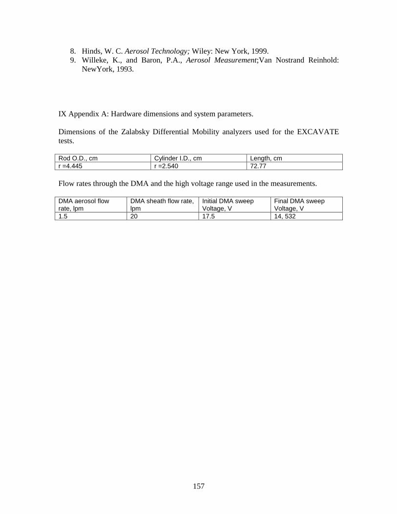
157

8. Hinds, W. C. Aerosol Technology; Wiley: New York, 1999. 9. Willeke, K., and Baron, P.A., Aerosol Measurement;Van Nostrand Reinhold:

NewYork, 1993. IX Appendix A: Hardware dimensions and system parameters. Dimensions of the Zalabsky Differential Mobility analyzers used for the EXCAVATE tests. Rod O.D., cm Cylinder I.D., cm Length, cm r =4.445 r =2.540 72.77 Flow rates through the DMA and the high voltage range used in the measurements. DMA aerosol flow rate, lpm

DMA sheath flow rate, lpm

Initial DMA sweep Voltage, V

Final DMA sweep Voltage, V

1.5 20 17.5 14, 532

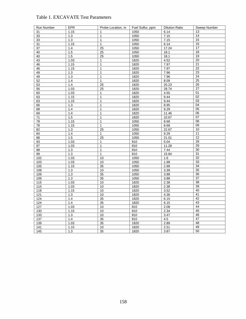
158

Table 1. EXCAVATE Test Parameters Run Number EPR Probe Location, m Fuel Sulfur, ppm Dilution Ratio Sweep Number 31 1.15 1 1050 6.14 13 33 1.3 1 1050 7.15 14 33 1.3 1 1050 7.15 15 31 1.15 1 1050 6.14 16 37 1.4 25 1050 17.24 17 40 1.5 25 1050 18.1 18 40 1.5 25 1050 18.1 19 43 1.03 1 1820 4.52 20 46 1.15 1 1820 7.97 21 46 1.15 1 1820 7.97 22 49 1.3 1 1820 7.96 23 49 1.3 1 1820 7.96 24 52 1.4 1 1820 8.09 25 53 1.4 25 1820 20.23 26 56 1.03 25 1820 28.74 27 60 1.03 1 1820 4.55 01 63 1.15 1 1820 9.44 02 63 1.15 1 1820 9.44 03 66 1.3 1 1820 8.95 04 68 1.4 1 1820 9.29 05 69 1.4 1 1820 11.46 06 71 1.5 1 1820 10.67 07 78 1.15 1 1050 8.68 08 78 1.15 1 1050 8.68 09 82 1.3 25 1050 22.67 10 84 1.4 1 1050 9.29 11 88 1.5 25 1050 21.01 12 93 1.03 1 810 5.04 28 97 1.03 1 810 11.28 29 98 1.3 1 810 7.44 30 99 1.3 1 810 15.84 31 102 1.03 10 1050 1.6 32 103 1.03 10 1050 1.98 33 105 1.15 35 1050 2.99 34 108 1.3 10 1050 3.39 35 109 1.3 35 1050 3.88 36 109 1.3 35 1050 3.88 37 115 1.03 10 1820 2.38 38 115 1.03 10 1820 2.38 39 118 1.15 10 1820 3.52 40 121 1.3 10 1820 4.36 41 124 1.4 35 1820 6.15 42 124 1.4 35 1820 6.15 43 127 1.03 10 810 2.08 44 130 1.15 10 810 2.34 45 133 1.3 10 810 3.47 46 137 1.4 35 810 4.5 47 139 1.03 35 1820 2.89 48 141 1.15 10 1820 2.51 49 145 1.3 35 1820 3.87 50

159

Table 2. EXCAVATE Statistical Data

Geometric Count Count Average Mass Mass Number Run Sweep Standard Standard Median Mode Mean Mass Median Mean Mass EI EI Number Number Deviation Deviation Dia., nm nm Dia., nm Dia., nm Dia., nm Dia., nm g/kg fuel #/kg fuel

31 13 23.8 1.1 30 23 33 42 61 68 6.02E-06 1.51E+16

33 14 32.4 1.2 37 28 42 55 83 95 2.66E-06 3.09E+15

33 15 36.1 1.2 40 30 46 60 92 106 3.46E-06 3.09E+15

31 16 43.4 1.1 47 36 53 69 102 116 5.03E-06 2.91E+15

37 17 21.7 1.4 22 12 30 58 151 208 2.12E-05 1.92E+16

40 18 42.3 1.2 44 30 53 77 134 162 2.90E-05 1.65E+16

40 19 42.3 1.2 43 28 53 81 153 188 2.95E-05 1.65E+16

43 20 48.5 1.2 49 34 58 84 143 171 1.31E-05 4.57E+15

46 21 14.8 1.3 19 12 23 37 76 96 7.89E-06 1.55E+16

46 22 13.5 1.2 18 12 23 34 62 77 3.88E-06 1.55E+16

49 23 34.7 1.1 39 30 44 58 87 99 1.18E-05 1.18E+16

49 24 36.8 1.2 40 30 46 62 96 111 1.45E-05 1.18E+16

52 25 44.0 1.2 46 35 54 72 112 129 2.16E-05 1.15E+16

53 26 46.4 1.2 48 35 56 76 122 142 1.53E-04 7.23E+16

56 27 48.5 1.2 50 38 58 78 121 140 3.25E-04 1.39E+17

60 1 36.8 1.4 33 17 46 90 248 347 4.66E-05 1.31E+16

63 2 29.2 1.2 33 25 39 52 82 95 6.11E-06 8.82E+15

63 3 30.4 1.2 35 26 40 54 83 96 6.40E-06 8.82E+15

66 4 38.1 1.2 41 30 48 65 101 118 9.49E-06 7.22E+15

68 5 41.7 1.2 44 31 51 71 116 137 1.59E-05 9.27E+15

69 6 41.9 1.2 44 33 51 70 110 128 1.98E-05 1.20E+16

71 7 45.5 1.2 47 35 55 75 119 138 2.91E-06 1.41E+16

78 8 25.4 1.3 27 16 35 58 126 162 1.96E-06 2.64E+15

78 9 27.7 1.3 30 19 37 58 114 142 2.13E-06 2.64E+15

82 10 49.2 1.1 52 40 59 76 111 126 2.94E-05 1.35E+16

84 11 42.0 1.2 44 32 52 71 112 131 5.48E-06 3.26E+15

88 12 45.6 1.2 48 36 55 74 113 130 6.96E-05 3.60E+16

93 28 20.7 1.2 26 20 30 40 61 70 3.07E-07 5.82E+14

97 29 20.9 1.3 24 15 30 48 95 120 1.25E-06 2.34E+15

98 30 37.3 1.2 41 31 47 62 93 107 1.05E-06 8.70E+14

99 31 38.1 1.2 41 30 48 65 103 119 4.88E-06 3.93E+15

102 32 14.4 1.3 18 12 23 36 69 85 3.25E-07 8.30E+14

103 33 3.4 1.1 12 11 13 14 16 17 1.43E-07 1.46E+15

105 34 4.8 1.0 14 12 14 15 17 18 1.17E-07 2.07E+15

108 35 36.4 1.2 39 27 46 67 116 139 1.91E-06 1.48E+15

109 36 32.6 1.3 33 21 42 69 141 180 2.54E-06 1.90E+15

109 37 33.6 1.3 34 22 43 68 135 170 2.67E-06 1.90E+15

115 38 49.9 1.5 39 17 60 140 500 763 9.87E-06 1.66E+15

115 39 25.1 1.5 21 9 32 74 260 395 5.36E-06 1.66E+15

118 40 31.9 1.2 35 24 41 59 100 120 3.04E-06 2.58E+15

121 41 41.1 1.2 44 33 51 68 105 122 3.61E-06 2.36E+15

124 42 42.8 1.2 45 33 52 71 112 130 6.48E-06 3.49E+15

124 43 26.0 1.5 24 11 36 77 245 360 4.35E-06 3.49E+15

127 44 45.0 1.2 47 35 55 73 114 132 2.58E-06 1.30E+15

130 45 36.6 1.1 41 32 46 59 85 96 1.28E-06 1.10E+15

133 46 38.6 1.2 41 30 48 67 109 128 2.18E-06 1.50E+15

137 47 49.1 1.2 50 37 58 79 123 143 5.61E-06 1.90E+15

139 48 7.6 1.1 14 11 16 21 30 33 8.38E-07 3.18E+15

141 49 34.2 1.1 39 30 44 56 81 92 1.30E-06 1.29E+15

145 50 42.9 1.2 46 34 52 70 106 123 3.11E-06 1.82E+15

160

Fig. 1. AEDC particulate probe (dimensions are in inches).

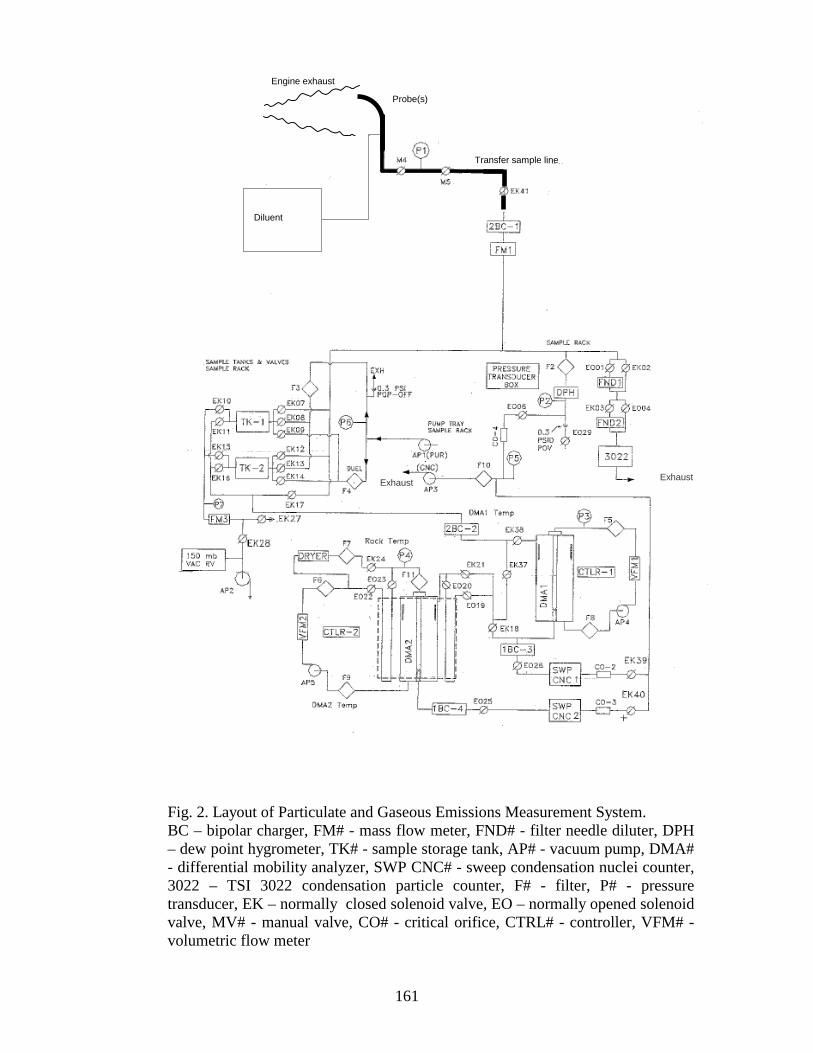
161

Fig. 2. Layout of Particulate and Gaseous Emissions Measurement System. BC – bipolar charger, FM# - mass flow meter, FND# - filter needle diluter, DPH – dew point hygrometer, TK# - sample storage tank, AP# - vacuum pump, DMA# - differential mobility analyzer, SWP CNC# - sweep condensation nuclei counter, 3022 – TSI 3022 condensation particle counter, F# - filter, P# - pressure transducer, EK – normally closed solenoid valve, EO – normally opened solenoid valve, MV# - manual valve, CO# - critical orifice, CTRL# - controller, VFM# - volumetric flow meter

Test cell wall

Exhaust Exhaust

Engine exhaust

Probe(s)

Dilution line

Transfer sample line

Diluent

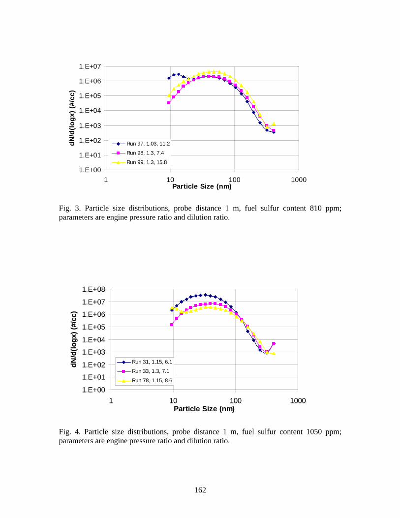
162

1.E+00

1.E+01

1.E+02

1.E+03

1.E+04

1.E+05

1.E+06

1.E+07

1 10 100 1000Particle Size (nm)

dN

/d(l

og

x) (

#/cc

)

Run 97, 1.03, 11.2

Run 98, 1.3, 7.4

Run 99, 1.3, 15.8

Fig. 3. Particle size distributions, probe distance 1 m, fuel sulfur content 810 ppm; parameters are engine pressure ratio and dilution ratio.

1.E+00

1.E+01

1.E+02

1.E+03

1.E+04

1.E+05

1.E+06

1.E+07

1.E+08

1 10 100 1000Particle Size (nm)

dN

/d(l

og

x) (

#/cc

)

Run 31, 1.15, 6.1

Run 33, 1.3, 7.1

Run 78, 1.15, 8.6

Fig. 4. Particle size distributions, probe distance 1 m, fuel sulfur content 1050 ppm; parameters are engine pressure ratio and dilution ratio.

163

1.E+00

1.E+01

1.E+02

1.E+03

1.E+04

1.E+05

1.E+06

1.E+07

1.E+08

1 10 100 1000Particle Size (nm)

dN

/d(l

og

x) (

#/cc

)

Run 49, 1.3, 7.9

Run 52, 1.4, 8.0

Run 63, 1.15, 9.4

Run 66, 1.3, 8.9

Run 68, 1.4, 9.2

Fig. 5. Particle size distributions, probe distance 1 m, fuel sulfur content 1820 ppm; parameters are engine pressure ratio and dilution ratio.

1.E+00

1.E+01

1.E+02

1.E+03

1.E+04

1.E+05

1.E+06

1.E+07

1.E+08

1 10 100 1000Particle Size (nm)

dN

/d(l

og

x) (

#/cc

)

Run 40, 1.5, 18.1

Run 88, 1.5, 21.0

Fig. 6. Particle size distributions, probe distance 25 m, fuel sulfur content 1050 ppm; parameters are engine pressure ratio and dilution ratio.

164

1.E+00

1.E+01

1.E+02

1.E+03

1.E+04

1.E+05

1.E+06

1.E+07

1.E+08

1 10 100 1000Particle Size (nm)

dN

/d(l

og

x) (

#/cc

)

Run 33, 1m, 7.1

Run 82, 25m, 22.6

Fig. 7. Particle size distributions, engine pressure ratio 1.3, fuel sulfur content 1050 ppm, parameters are probe distance and dilution ratio.

1.E+00

1.E+01

1.E+02

1.E+03

1.E+04

1.E+05

1.E+06

1.E+07

1.E+08

1 10 100 1000Particle Size (nm)

dN

/d(l

og

x) (

#/cc

)

Run 33, 1050 ppm, 7.1Run 49, 1820 ppm, 7.9

Run 66, 1820 ppm, 8.9Run 98, 810 ppm, 7.4Run 99, 810 ppm, 15.8

Fig. 8. Particle size distributions, engine pressure ratio 1.3, probe distance 1 m, parameters are fuel sulfur content, and dilution ratio.

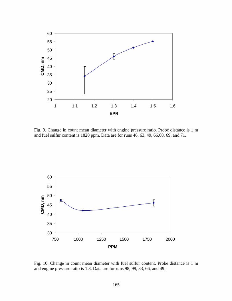
165

20

25

30

35

40

45

50

55

60

1 1.1 1.2 1.3 1.4 1.5 1.6

EPR

CM

D, n

m

Fig. 9. Change in count mean diameter with engine pressure ratio. Probe distance is 1 m and fuel sulfur content is 1820 ppm. Data are for runs 46, 63, 49, 66,68, 69, and 71.

30

35

40

45

50

55

60

750 1000 1250 1500 1750 2000

PPM

CM

D, n

m

Fig. 10. Change in count mean diameter with fuel sulfur content. Probe distance is 1 m and engine pressure ratio is 1.3. Data are for runs 98, 99, 33, 66, and 49.

166

1.00E+05

5.10E+06

1.01E+07

1.51E+07

2.01E+07

2.51E+07

1 1.1 1.2 1.3 1.4 1.5

Engine Pressure Ratio

To

tal,

#/cc

Fig. 11. Change in total particle number density with engine pressure ratio. Total number densities are averages of run 63, 46, 66, 49, 68 and 52.

1.00E+05

4.10E+06

8.10E+06

1.21E+07

1.61E+07

2.01E+07

2.41E+07

0 500 1000 1500 2000

Sulfur Content, ppm

To

tal,

#/cc

Fig. 12. Change in total particle number density with fuel sulfur content. Total number densities are averages of run 98, 99, 33, 66, and 49.

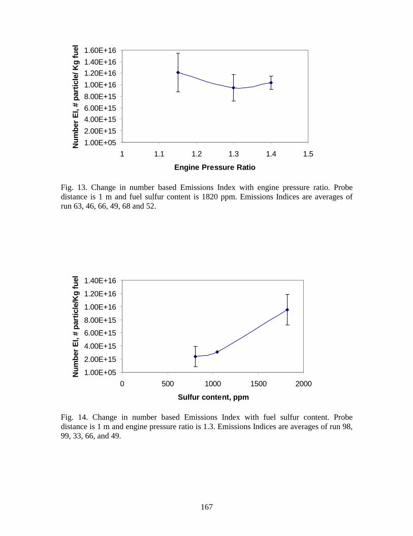
167

1.00E+05

2.00E+15

4.00E+15

6.00E+15

8.00E+15

1.00E+16

1.20E+16

1.40E+16

1.60E+16

1 1.1 1.2 1.3 1.4 1.5

Engine Pressure Ratio

Nu

mb

er E

I, #

par

ticl

e/ K

g f

uel

Fig. 13. Change in number based Emissions Index with engine pressure ratio. Probe distance is 1 m and fuel sulfur content is 1820 ppm. Emissions Indices are averages of run 63, 46, 66, 49, 68 and 52.

1.00E+05

2.00E+15

4.00E+15

6.00E+15

8.00E+15

1.00E+16

1.20E+16

1.40E+16

0 500 1000 1500 2000

Sulfur content, ppm

Nu

mb

er E

I, #

par

ticl

e/K

g f

uel

Fig. 14. Change in number based Emissions Index with fuel sulfur content. Probe distance is 1 m and engine pressure ratio is 1.3. Emissions Indices are averages of run 98, 99, 33, 66, and 49.

168

5.00E-06

7.00E-06

9.00E-06

1.10E-05

1.30E-05

1.50E-05

1.70E-05

1 1.1 1.2 1.3 1.4 1.5

Engine Pressure Ratio

Mas

s E

I, g

/kg

fu

el b

urn

ed

Fig. 15. Change in mass based Emissions Index with engine pressure ratio. Probe distance is 1 m and fuel sulfur content is 1820 ppm. Emissions Indices are averages of run 63, 46, 66, 49, 68 and 52.

5.00E-07

2.50E-06

4.50E-06

6.50E-06

8.50E-06

1.05E-05

0 500 1000 1500 2000

Sulfur Content, ppm

Mas

s E

I, g

/kg

fu

el b

urn

ed

Fig. 16. Change in mass based Emissions Index with fuel sulfur content. Probe distance is 1 m and engine pressure ratio is 1.3. Emissions Indices are averages of run 98, 99, 33, 66, and 49.

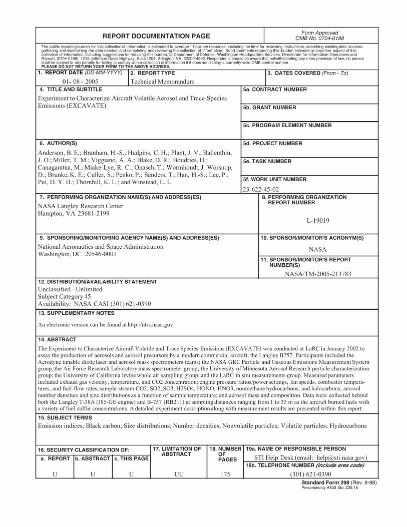
REPORT DOCUMENTATION PAGE Form ApprovedOMB No. 0704-0188

2. REPORT TYPE

Technical Memorandum 4. TITLE AND SUBTITLE

Experiment to Characterize Aircraft Volatile Aerosol and Trace-Species Emissions (EXCAVATE)

5a. CONTRACT NUMBER

6. AUTHOR(S)

Anderson, B. E.; Branham, H.-S.; Hudgins, C. H.; Plant, J. V.; Ballenthin, J. O.; Miller, T. M.; Viggiano, A. A.; Blake, D. R.; Boudries, H.; Canagaratna, M.; Miake-Lye, R. C.; Onasch, T.; Wormhoudt, J. Worsnop, D.; Brunke, K. E.; Culler, S.; Penko, P.; Sanders, T.; Han, H.-S.; Lee, P.; Pui, D. Y. H.; Thornhill, K. L.; and Winstead, E. L.

7. PERFORMING ORGANIZATION NAME(S) AND ADDRESS(ES)

NASA Langley Research CenterHampton, VA 23681-2199

9. SPONSORING/MONITORING AGENCY NAME(S) AND ADDRESS(ES)

National Aeronautics and Space AdministrationWashington, DC 20546-0001

8. PERFORMING ORGANIZATION REPORT NUMBER

L-19019

10. SPONSOR/MONITOR'S ACRONYM(S)

NASA

13. SUPPLEMENTARY NOTES

An electronic version can be found at http://ntrs.nasa.gov

12. DISTRIBUTION/AVAILABILITY STATEMENTUnclassified - UnlimitedSubject Category 45Availability: NASA CASI (301) 621-0390

19a. NAME OF RESPONSIBLE PERSON

STI Help Desk (email: help@sti.nasa.gov)

14. ABSTRACT

The Experiment to Characterize Aircraft Volatile and Trace Species Emissions (EXCAVATE) was conducted at LaRC in January 2002 to assay the production of aerosols and aerosol precursors by a modern commercial aircraft, the Langley B757. Participants included the Aerodyne tunable diode laser and aerosol mass spectrometers teams; the NASA GRC Particle and Gaseous Emissions Measurement System group; the Air Force Research Laboratory mass spectrometer group; the University of Minnesota Aerosol Research particle characterization group; the University of California Irvine whole air sampling group; and the LaRC in situ measurements group. Measured parameters included exhaust gas velocity, temperature, and CO2 concentration; engine pressure ratios/power settings, fan speeds, combustor tempera- tures, and fuel-flow rates; sample stream CO2, SO2, SO3, H2SO4, HONO, HNO3, nonmethane hydrocarbons, and halocarbons; aerosol number densities and size distributions as a function of sample temperature; and aerosol mass and composition. Data were collected behind both the Langley T-38A (J85-GE engine) and B-757 (RB211) at sampling distances ranging from 1 to 35 m as the aircraft burned fuels with a variety of fuel sulfur concentrations. A detailed experiment description along with measurement results are presented within this report.

15. SUBJECT TERMS

Emission indices; Black carbon; Size distributions; Number densities; Nonvolatile particles; Volatile particles; Hydrocarbons

18. NUMBER OF PAGES

175

19b. TELEPHONE NUMBER (Include area code)

(301) 621-0390

a. REPORT

U

c. THIS PAGE

U

b. ABSTRACT

U

17. LIMITATION OF ABSTRACT

UU

Prescribed by ANSI Std. Z39.18Standard Form 298 (Rev. 8-98)

3. DATES COVERED (From - To)

5b. GRANT NUMBER

5c. PROGRAM ELEMENT NUMBER

5d. PROJECT NUMBER

5e. TASK NUMBER

5f. WORK UNIT NUMBER

23-622-45-02

11. SPONSOR/MONITOR'S REPORT NUMBER(S)

NASA/TM-2005-213783

16. SECURITY CLASSIFICATION OF:

The public reporting burden for this collection of information is estimated to average 1 hour per response, including the time for reviewing instructions, searching existing data sources, gathering and maintaining the data needed, and completing and reviewing the collection of information. Send comments regarding this burden estimate or any other aspect of this collection of information, including suggestions for reducing this burden, to Department of Defense, Washington Headquarters Services, Directorate for Information Operations and Reports (0704-0188), 1215 Jefferson Davis Highway, Suite 1204, Arlington, VA 22202-4302. Respondents should be aware that notwithstanding any other provision of law, no person shall be subject to any penalty for failing to comply with a collection of information if it does not display a currently valid OMB control number.PLEASE DO NOT RETURN YOUR FORM TO THE ABOVE ADDRESS.

1. REPORT DATE (DD-MM-YYYY)

08 - 200501-