NBER WORKING PAPER SERIES

EXPENDITURE VISIBILITY AND CONSUMER BEHAVIOR:NEW EVIDENCE

Ori Heffetz

Working Paper 25161http://www.nber.org/papers/w25161

NATIONAL BUREAU OF ECONOMIC RESEARCH1050 Massachusetts Avenue

Cambridge, MA 02138October 2018

I thank participants in the Cornell Behavioral/Experimental Economics Lab Meetings for useful early feedback and ideas, Cornell’s Survey Research Institute for conducting the telephone survey, Nadia Streletskaya and Lin Xu for programming the web survey, Inbal Dekel, Matan Gibson, Ofer Glicksohn, Guy Ishai, and Daniel Reeves for providing excellent research assistance, and Eve Sihra and conference/seminar participants at the Princeton Workshop on Public Economics, Stanford Institute for Theoretical Economics, Bar-Ilan U, Ben-Gurion U, and UC Berkeley for helpful comments. This research project was supported by the Israel Science Foundation (grant no. 1680/16), and by the S.C. Johnson Graduate School of Management. The views expressed herein are those of the author and do not necessarily reflect the views of the National Bureau of Economic Research.

NBER working papers are circulated for discussion and comment purposes. They have not been peer-reviewed or been subject to the review by the NBER Board of Directors that accompanies official NBER publications.

© 2018 by Ori Heffetz. All rights reserved. Short sections of text, not to exceed two paragraphs, may be quoted without explicit permission provided that full credit, including © notice, is given to the source.

Expenditure Visibility and Consumer Behavior: New EvidenceOri HeffetzNBER Working Paper No. 25161October 2018JEL No. D12,D83,D91,Z13

ABSTRACT

Expenditure visibility—the extent to which a household’s spending on a consumption category is noticeable to others—is measured in three new surveys, with ~3,000 telephone and online respondents. Visibility shows little change across time (ten years) and survey methods. Four different notions, or dimensions, of visibility are measured: the noticeability of above-average spending on a category; that of below-average spending; and the positivity/negativity of impressions made by above- and below-average spending. Jointly, these visibility measures explain up to three quarters or more of the observed variation in total-expenditure elasticities across consumption categories in U.S. data. Possible theoretical explanations are explored.

Ori HeffetzS.C. Johnson Graduate School of ManagementCornell University324 Sage HallIthaca, NY 14853and The Hebrew University of Jerusalemand also NBERoh33@cornell.edu

1 Introduction

The sociocultural visibility of consumer expenditures has for centuries been considered an

important determinant of consumer behavior.1 Intuitively, one’s costly diamond is more

conspicuous to others than one’s costly life-insurance policy—a difference that could explain

differences in demand patterns across the two commodities. The theoretical implications of

this intuition have been investigated in modern consumer-choice theory (e.g., Frank 1985,

Ng 1987, Ireland 1994). Empirical applications, however, require substituting intuition with

more systematic data that would place different expenditures on a quantitative visibility

scale. A diamond and an insurance policy may be easy to place, somewhere close to extreme

visibility and non-visibility, respectively; but how visible are expenditures on housing, health,

education, or charity? And how stable are measures of their visibility—do they change over

time, across survey methods, or across visibility-definition variations? Most importantly,

how much does it all matter for explaining household expenditure patterns? Relevant data

for answering these questions have only recently started to be collected. As discussed shortly,

while researcher demand is rising, supply is still limited.

This paper’s contribution is twofold: it collects new data to help address the data gap; and

it applies its new data to help explain household consumption behavior. Its first part intro-

duces three new visibility surveys, conducted in 2014–2015 among ∼3,000 U.S. respondents.

They replicate existing visibility measures and, more importantly, generate new measures

that are readily applicable in empirical work. The paper’s second part imports these new

measures into an existing application, and finds that they dramatically increase our power

to explain observed cross-commodity variation in total-expenditure elasticities.

Table 1’s top panel summarizes published efforts to date to measure expenditure visibility

with surveys. The earliest (from the mid-1990s) is an informal survey of twenty female

students, measuring the social visibility of four cosmetics products (Chao and Schor 1998).

It was followed in 2004 by a random-digit-dialing (RDD) telephone survey of 480 adults

in the continental U.S. (Heffetz 2011). This 2004 survey was the first generally applicable,

1Smith, Marx, Veblen, Duesenberry, and many others wrote famous passages or entire books on socialcomparisons and signaling, in the specific context of consumer expenditures. Social comparisons/signalingmore generally, as well as public display vs. private behavior, pride vs. modesty (or shame), and appearancevs. truth, feature heavily in the writings of much earlier authors, such as Plato.

2

national visibility survey; it asked respondents how quickly they would notice a newly met

person’s above-average expenditures on each of 31 consumption categories that together cover

virtually the entire basket of U.S. household expenditures in the Bureau of Labor Statistics’s

Consumer Expenditure Survey (CEX). Several later surveys were conducted online, using

convenience samples of students. They include a 2007 survey inspired by the 2004 survey,

asking 320 students a similar question about above-average expenditures, but replacing speed

of noticing with closeness of interaction, and reclassifying the 31 CEX categories into 18

(Charles et al. 2009); a 2010 replication in India of the 2007 survey, asking 163 students

regarding 20 categories from the India Human Development Survey (IHDS; Khamis et al.

2012); and a 2011 survey of 108 students in Germany, asking which of a collection of 16

items are easily observable (Hillesheim and Mechtel 2013).

Table 1: Visibility Surveys

Year Described in N Sample Mode Expendituresa

≤1996 Chao & Schor (1998) 20 Female Harvard students Informal 4 Cosmetics2004/5 Heffetz (2011) 480 RDD Cont. U.S. (18+) Telephone 31 CEX2007 Charles et al. (2009) 320 UChicago grad students Online 18 CEX2010 Khamis et al. (2012) 163 Delhi Sc. Econ. students Online 20 IHDS2011 Hillesheim & Mechtel (2013) 108 U of Tubingen students Online 16 Various

2014 }This paper

500 RDD Cont. U.S. (18+) Telephone }31 CEX

2014 1,079b }ClearVoice U.S. (18+)

}Online

2015 1,426c 17 Clothing CEX

aCosmetics: lipstick, mascara, eyeshadow, and facial cleanser. CEX: broad categories from the U.S.Consumer Expenditure Survey. IHDS: broad categories from the India Human Development Survey. Various:a mix of expenditures, income, vacation/leisure time, and personal characteristics (e.g., attractiveness).Clothing CEX: clothing-only expenditure subcategories in the CEX.

bFour different visibility treatments, between-subjects design.cTwo different visibility treatments, between-subjects design.

These surveys were motivated by research questions closely related to Veblen’s (1899)

idea that the rich advertise their wealth by conspicuously consuming more than others.

They therefore focus on measuring a specific notion of visibility: the noticeability of larger-

than-average spending. But the measures they provide have been used in a broader set

of subsequent empirical applications. The 2004 and 2007 U.S./CEX visibility measures

have been used, for example, to assess whether consumption utility is relative vs. absolute

(Kamakura and Du 2012); to investigate the importance of conspicuous consumption under

3

alternative political regimes (East vs. West Germany after reunification, Friehe and Mechtel

2014); to investigate the links from inequality in visible expenditure to violent crime (Hicks

and Hicks 2014), and from property crime to distortions in conspicuous- vs. inconspicuous-

consumption allocation decisions (Mejıa and Restrepo 2016); to assess the hypothesis of

“trickle-down consumption,” i.e., that rising income and consumption among high-income

households since the early 1980s have induced lower-income households to consume a larger

share of their income (Bertrand and Morse 2016); and to distinguish between alternative

mechanisms that may drive consumption network/peer effects (De Giorgi, Frederiksen, and

Pistaferri 2016). These U.S. visibility measures have in addition been used in other recent

applications in more limited ways, e.g., to classify particular expenditures as high- or low-

visibility. For example, Cosaert (2018) estimates the diamondness (Ng 1987) of more and

less visible goods. Finally, the 2010 India/IHDS measure is starting to be used as well (e.g.,

Jaikumar and Sarin 2015, Bellet and Sihra 2018).

Table 1’s bottom panel lists the three new U.S. visibility surveys introduced in this

paper’s first part. We provide full details in section 2. The first new survey is a 2014

national telephone survey that replicates the 2004 survey, resulting in a second comparable

datapoint, ten years apart. It thus provides evidence on the stability of the original survery-

based visibility measure and, therefore, on the robustness of findings across the above range

of applications that use the original 2004 measure. The second and third are new web surveys

conducted in 2014 and 2015, respectively. Relative to the first 2014 survey, they vary the

interview mode—online vs. telephone—and the national survey sample type—convenience

vs. RDD. Relative to each other, they vary the set of expenditures and its granularity, using

the original 31 broad CEX categories (in 2014) vs. a new set of 17 clothing-only subcategories

(in 2015).

Most importantly, the new online surveys vary the visibility question itself, including four

(in 2014) and two (in 2015) different question variants, aimed to measure different notions of

visibility. Therefore, in addition to providing evidence on the sensitivity of visibility measures

to underlying survey-implementation details, these new surveys generate measures of notions

of visibility that have not been previously measured. The new measures are designed to be

both compatible with past applications and readily applicable in future ones.

4

Section 3 analyzes the data from the new surveys. Three main findings are highlighted,

along with their implications for empirical research. First, using the original 2004 visibil-

ity question, we record remarkable stability in results across the 2004 and 2014 telephone

surveys (correlation = 0.99 across the two benchmark visibility measures; N = 31 expen-

ditures). Such stability, ten years and many technology-based sociocultural developments

apart, suggests that the empirical work above that uses visibility measures is on rather sta-

ble grounds. In particular, it allays potential concerns regarding those of the papers (e.g.,

Bertrand and Morse, 2016) that match 2004 visibility data with expenditure data dating

back to 1980, i.e., almost a quarter-century earlier.

Second, we similarly record stability across the two telephone surveys and the 2014 online

survey (correlation = 0.97 across either the 2004 or 2014 telephone visibility measure and

the online measure). Overall, these two findings suggest that the original visibility question

captures a stable property of expenditures, that has not recently changed much across time

(10 years) and technology, and that appears largely invariant to interview mode and survey

sample. This in turn opens the door for data-collection efforts to measure new notions of

visibility and track them over time; such efforts need be neither frequent nor expensive.2

The third finding, and the main contribution of this paper’s first part (i.e., the data part),

relates to such new notions of visibility that the 2014–2015 online surveys measure for the first

time. They expand the main visibility notion that has been measured and used to date—an

upward noticeability notion, based on a question about the noticeability of more-than-average

expenditures, referred to below as a Notice More (NM) question.3 The new notions are

based on a question about the noticeability of less-than-average expenditures (Notice Less,

NL), measuring downward noticeability ; and two questions about the positivity/negativity of

impressions made by more- and less-than-average expenditures, conditional on their being

noticed (Impressions More and Less, IM and IL).

The 2014 online survey thus has a 2×2 between-subjects design, yielding four visibility

measures: NM, NL, IM, and IL; the 2015 clothing-only survey focuses on NM and NL. The

2The cost per respondent in the 2014 national RDD telephone survey was roughly twenty times higherthan that in the 2014 online survey. Such a cost multiple appears typical.

3Versions of such an NM question are used in the 2004, 2007, and 2010 surveys in table 1’s top panel(and in all the new surveys in its bottom panel). For the different versions’ wordings, see subsection 2.1.2.

5

new measures are motivated by the idea that spending more vs. less than average on a com-

modity may be differently noticeable and may make different impressions conditionally on

being noticed. Indeed, unlike the first two findings above—of close to perfect correlations

(0.97–0.99) across replications of the NM question that differ in survey mode, sample, and

decade—the correlations across the four randomly assigned treatments within the same 2014

survey are lower, varying in absolute value from 0.42 to 0.92. The lower correlations, and

a qualitative expenditure-by-expenditure assessment of the four measures (in section 3.2),

suggest that the new questions do capture distinct notions, or aspects, of visibility, not pre-

viously measured. This in turn raises the possibility that models and empirical applications

of consumer behavior that incorporate visibility but only consider NM visibility may miss

an important part of the story. This possibility is investigated next, in the context of one

application.

The paper’s second part demonstrates that the new visibility measures can substantially

increase the explained portion of cross-expenditure variation in demand patterns.4 It focuses

on the empirical attempt to explain cross-expenditure variation in Engel curves—specifically,

in income elasticities—with measurable properties of expenditures. In their “Retrospectives:

Engel Curves,” Chai and Moneta (2010) observe that such an explanation has not yet been

offered, and comment: “it may be tempting to conclude, as Houthakker (1967 [1992]) did,

that any proper explanation of variation observed in Engel curves requires researchers to go

‘far outside economics.’” However, as mentioned in the opening paragraph above, economic

models have incorporated a broader set of topics since Houthakker’s pessimistic prediction

half a century ago. A Stone-Geary application of Ireland’s (1994) conspicuous consumption

model, for example, endogenously predicts income elasticity to be higher if a good is visible

and lower if it is not—as shown in Heffetz (2011), where it is also shown empirically that

income elasticities can indeed be predicted from NM visibility.

Section 4 demonstrates the value for empirical research of the new visibility measures by

revisiting that application (for which the 2004 visibility survey was originally conducted).

The original main finding was that weighted univariate OLS regressions of the total-expenditure

4As discussed shortly, “explained portion” here refers to R2 in a linear regression. No causality inferencesare implied. Indeed, the possibility of reverse causality is explored formally in section 5.

6

elasticities of 29 expenditure categories on their NM visibility measure result in large co-

efficients and, importantly, high R2’s. A benchmark whole-population specification had

R2 = 0.18, meaning that one-sixth to one-fifth of the cross-expenditure variation in elastici-

ties was explained by the 2004 NM visibility measure alone (the top three income quintiles

had R2’s in the range 0.19–0.32). Section 4 first replaces the original 2004 (telephone) NM

measure with the 2014 (online) NM measure, and the original CEX expenditure data with

updated expenditure data on 31 categories, and essentially replicates the original findings

(R2 = 0.17; top quintiles’ R2 = 0.19–0.28). It then adds the new NL, IM, and IL measures

as additional (or alternative) regressors.

Section 4’s main finding is that in multivariate regressions on more than one visibil-

ity measure, explanatory power increases dramatically. With two regressors—NM and

NL, or NM and IM—R2 = 0.43–0.59 (top two quintiles: 0.55–0.68); with all four regres-

sors, R2 = 0.73 (0.80–0.81). Moreover, the coefficient estimates suggest that the differ-

ence NM−NL strongly predicts elasticities. We argue that this difference (between upward

and downward noticeability) may capture noticeability’s discretionary, or active component.

The replicability and robustness of these findings are demonstrated using CEX data on 17

clothing-only subcategories and the new 2015 NM and NL clothing-only visibility measures.

Section 5 presents two stylized formal examples that explore the potential role of causal-

ity in these NM−NL findings. The examples offer potential explanations in both directions:

from visibility to high elasticity—with an alternative to Ireland’s model (since it cannot

accommodate the difference between upward and downward visibility)—and from high elas-

ticity to visibility—i.e., a reverse-causality interpretation. They are used to interpret the

empirical findings, and to conclude that while strong visibility-elasticity associations are a

robust empirical fact, its underlying mechanism remains an open question for future research.

Section 6 concludes.

2 Three New Visibility Surveys: Design

This paper’s new visibility surveys share the common structure of past surveys. It is based on

two components: a list of expenditure categories, and a visibility question. Each respondent

7

answers the visibility question repeatedly, each time for a different expenditure category

from the list, until the list is exhausted.

2.1 2014 Telephone and Online Surveys

As the bottom panel of table 1 shows, this paper’s two new 2014 surveys differ in interview

mode and survey sample. However, they are identical in the list of 31 expenditures they

ask about, and they share a similar NM (Notice More) visibility question, which they also

share with the original 2004 survey. In addition, the 2014 online survey includes three new

visibility questions. We now discuss these survey-design details.

2.1.1 31 Expenditure Categories

Table 2 lists the 31 expenditure categories that respondents are asked about in the 2014

telephone and online surveys. The list is identical to the original 2004 list in all but two

categories: Ot1 and Ot2 (rows 28 and 29); for these, the table also lists the two original 2004

categories, for comparison. The 2004 list was based on Harris and Sabelhaus’s (2005) list

of consumption categories, that was designed to cover virtually all expenditures in the raw

CEX (Interview Survey) data.

Appendix A.1 provides detail regarding the construction of the 2014 category list from

the 2004 list. Here we note, first, that as with the original 2004 list, the order of words

in each category’s description reflects the relative empirical importance (in the CEX data)

of the items within that category. Second, we note that although the decade that followed

2004 saw many newly available goods and services replace older ones within many of the

31 categories, all but two of the original category descriptions are sufficiently broad to be

unaffected. The two exceptions underwent only minuscule modifications, related to specific

technologies mentioned in their descriptions (e.g., CDs, internet).

2.1.2 Notice More (NM) Question

Figure 1 reproduces a screenshot of the 2014 online survey’s Notice More (NM) question.

It is identical to the question in the 2014 telephone survey, which in turn is identical to

8

Table 2: Expenditure Categories in 2014 Surveys

1. FdH food and nonalcoholic beverages at grocery, specialty and convenience stores.2. FdO dining out at restaurants, drive-thrus, etc, excl. alcohol; incl. food at school.3. Cig tobacco products like cigarettes, cigars, and pipe tobacco.4. AlH alcoholic beverages for home use.5. AlO alcoholic beverages at restaurants, bars, cafeterias, cafes, etc.6. Clo clothing and shoes, not including underwear, undergarments, and nightwear.7. Und underwear, undergarments, nightwear and sleeping garments.8. Lry laundry and dry cleaning.9. Jwl jewelry and watches.10. Brb barbershops, beauty parlors, hair dressers, health clubs, etc.11. Hom rent, or mortgage, or purchase, of their housing.12. Htl lodging away from home on trips, and housing for someone away at school.13. Fur home furnishings and household items, like furniture, appliances, tools, linen.14. Utl home utilities such as electricity, gas, and water; garbage collection.15. Tel home telephone services, not including mobile phones.16. Cel mobile phone services.17. HIn homeowners insurance, fire insurance, and property insurance.18. Med medical care, incl. health insurance, drugs, dentists, doctors, hospitals, etc.19. Fee legal fees, accounting fees, and occupational expenses like tools and licenses.20. LIn life insurance, endowment, annuities, and other death-benefits insurance.21. Car the purchase of new and used motor vehicles such as cars, trucks, and vans.22. CMn vehicle maintenance, mechanical and electrical repair and replacement.23. Gas gasoline and diesel fuel for motor vehicles.24. CIn vehicle insurance, like insurance for cars, trucks, and vans.25. Bus public transportation, both local and long distance, like busses and trains.26. Air airline fares for out-of-town trips.27. Bks books incl. school books, newspapers and magazines, toys, games, and hobbies.28. Ot1 computers, TVs, visual, audio, musical and sports equipment, music, games, etc.

(Ot1 in 2004 computers, games, TVs, video, audio, musical and sports equipment, tapes, CDs.)29. Ot2 cable TV, internet, pets and veterinarians, sports, country clubs, movies, concerts.

(Ot2 in 2004 cable TV, pets and veterinarians, sports, country clubs, movies, and concerts.)30. Edu education, from nursery to college, like tuition and other school expenses.31. Cha contributions to churches or other religious organizations, and other charities.

9

that in the original 2004 telephone survey. While the language surrounding its response

options is slightly adjusted to improve on-screen readability in the online version, the five

response options themselves do not change.5 In all surveys, respondents answer this question

31 times, each time with one of the 31 expenditure categories from table 2 appearing where

the category “jewelry and watches” appears in figure 1. The order of the 31 categories is

randomized for each respondent.

The question asks respondents regarding quickness of noticing an above-average expen-

diture of a newly met person who lives in a household similar to the respondent’s. The focus

on a similar-household person is motivated by both relevance and practicality: social (non-

family) interactions often involve people of roughly similar neighborhood, age, education,

income, household composition, etc., and it makes little sense to ask, e.g., a young, urban,

unmarried male about the expenditures of a retired rural couple (for further discussion and

a formal model, see Heffetz 2012, section 3.2). Importantly, the question conveys that the

reason for said above-average expenditure is tastes rather than needs : “they like to, and do,

spend more.” In effect, respondents are asked to imagine a tastes-driven exogenous shock

to a typical similar household’s expenditure. This is important because some expenditures

(e.g., medical care) could be above average due to a need (e.g., deteriorating health), in which

case they may be noticed quickly due to the noticeability of the circumstances rather than

that of the expenditure itself. The question’s wording aims to mitigate this potential issue.

5Specifically, the original response options were read as a follow-up question by the telephone interviewer:

“Would you notice it almost immediately upon meeting them for the first time, a short whileafter, a while after, only a long while after, or never?”

As figure 1 shows, the online response options start with the self-statement “I would notice it. . . ” andcontain slightly more repetition. The only purpose of this adjustment is to make the question as clear aspossible in the online version where—in contrast with the telephone version—respondents do not have achance to ask an interviewer for clarification.

For completeness and comparison, we also reproduce here the wording in the other U.S./CEX survey listedin table 1’s top panel, namely the 2007 survey (Charles et al. 2009, robustness appendix):

“Consider a person who lives in a household and community roughly similar to yours. Howclosely would you have to interact with this person in order to observe that they consistentlyspend more than average on each of the following categories?”

Response options in that survey “ranged from 1 (indicating that higher than average spending could beobserved if the respondent did not interact socially with the person at all) to 5 (indicating that spendingwould never be observed).”

Finally, the wording in the 2010 survey that was conducted in India (Khamis et al., 2012; see table 1)combines elements from both the 2004 and 2007 surveys.

10

Figure 1: 2014 Online Survey, Notice More (NM) Question

2.1.3 Notice Less (NL), Impressions More (IM), and Impressions Less (IL)

Unlike the 2004 and 2014 telephone surveys, which include only the above Notice More (NM)

question, the 2014 online survey includes three additional question versions:

Notice Less (NL): identical to the NM version in figure 1, except for one word; “more”

(third line, first word) is replaced with “less.” This version therefore asks how quickly

one would notice spending less than average on a category.

Impressions More (IM): see figure 2 for a screenshot. The first two sentences are identical

to those in the NM version, and the rest of the question is modified. Instead of asking

respondents how quickly they would notice an above-average expenditure, respondents

are asked whether and how their views/impressions would be affected conditionally on

noticing it.

Impressions Less (IL): identical to the IM version in figure 2, except for one word; “more”

(third line, first word) is replaced with “less.” This version therefore asks whether and

11

how one’s impressions would be affected by noticing spending less than average on a

category.

Figure 2: 2014 Online Survey, Impressions More (IM) Question

The 2014 online survey thus has a 2×2 between-subjects design: each respondent is

randomly assigned to one of the four versions [Impressions vs. Notice]×[More vs. Less].

They then answer their assigned question version for each of the 31 expenditure categories

(randomly ordered).

The discussion above regarding the wording of the NM question can now be generalized.

The phrase “they like to, and do” remains unchanged in all four versions, conveying a

shock to tastes rather than to needs. This becomes even more important for the NL than

for the NM question, as spending less than average on an expenditure could simply result

from a lower-than-average budget (which, again, may itself be visible, e.g., due to visible

circumstances). Furthermore, when asking about respondents’ impressions of someone who

spends more/less than average on a category (IM and IL), it is important to clarify that the

spender is driven by tastes rather than needs.

12

2.2 2015 Online Clothing-Only Survey

Clothing as an expenditure category plays a central role in socioculturally-related consump-

tion. Constantly changing social and cultural conventions prescribe different clothing for

different circumstances, depending on occasion, event, date, social position, professional

role, gender, age, culture, and place. As fashions change, what was acceptable yesterday

may be (socioculturally) unwearable today. Beyond its sociocultural role, however, clothing

is a relatively homogenous expenditure category in terms of its production processes and

materials, durability, availability to consumers, and its main (non-sociocultural) purpose,

i.e., covering and protecting the wearer’s body. At the same time, expenditures on different

clothing subcategories are not all equally noticeable and are therefore not all equally subject

to sociocultural considerations.

Of the 31 expenditure categories in table 2, two cover clothing. Together, the two ag-

gregate data on more than 70 individual CEX expenditure items. Table 3 presents a finer

reclassification of these items into 17 clothing-only subcategories.6 The third new survey

introduced in this paper (see table 1’s bottom row) repeats the 2014 online survey’s NM and

NL treatments, but uses these 17 clothing-only subcategories (randomly ordered). The clas-

sification into these subcategories (in table 3) reflects an attempt to balance two opposing

considerations: on the one hand, an aspiration to classify into a separate subcategory any

item that may differ in visibility from other items; on the other hand, a need to avoid sub-

categories that are so specific that few households in the CEX data spend positive amounts

on them.7

6The two clothing categories in table 2 are Clo (row 6, “clothing and shoes, not including underwear,undergarments, and nightwear”) and Und (row 7, “underwear, undergarments, nightwear and sleeping gar-ments”). The seventeen subcategories in table 3 include fourteen that disaggregate Clo, plus the followingthree that disaggregate Und: nightwear (Nwr, row 8), socks (Soc, row 15), and underwear (Uwr, row 17).

7The clothing-only survey does not include IM and IL treatments. This design decision, namely, to refrainfrom asking about positive/negative impressions in the clothing context, aims to avoid unintentionally makingrespondents feel uncomfortable. For example, it aims to avoid asking about impressions related to noticingthat someone spent more or less on clothing subcategories explicitly assigned to men, women, boys, girls,or infants, as such impression questions may have unintended connotations. (Sex/age-based subcategoriesconstitute more than half of the 17 subcategories in table 3, as it seemed plausible at the survey-design stagethat they may have different visibility levels.)

13

Table 3: Clothing-Only Expenditure Subcategories in 2015 Survey

1. Acc clothing accessories like belts, purses, scarves, hats, EXCLUDING jewelry/shoes.2. Sts suits, sport coats, and tailored jackets (for men and women).3. Boy boys’ clothes like pants, shorts, shirts, and sweaters, EXCLUDING shoes.4. Grl girls’ clothes like shirts, pants, shorts, dresses, and skirts, EXCLUDING shoes.5. Men men’s clothes like pants, shorts, shirts, sweaters and vests, EXCLUDING shoes.6. Wmn women’s clothes like pants, shorts, dresses, shirts, and sweaters, EXCL. shoes.7. Inf infants’ diapers and clothes, including outerwear, accessories, and footwear.8. Nwr nightwear such as pajamas and robes.9. Oth sewing/quilting materials, luggage, luggage carriers, wigs, and hairpieces.10. Owr outerwear like coats, jackets and furs.11. ShB boys’ shoes.12. ShG girls’ shoes.13. ShM men’s shoes.14. ShW women’s shoes.15. Soc socks, stockings and hose (for men and women).16. Spo athletic clothing like swimsuits, warm-up suits, and uniforms, EXCLUDING shoes.17. Uwr underwear and undergarments, EXCLUDING socks.

3 New Visibility Measures: Results

The 2014 telephone survey was conducted by the Survey Research Institute (SRI) at Cornell

University from May 3 to 29, 2014. The phone sample, provided to SRI by Marketing

Systems Group, is a random-digit-dial (RDD) list of cellphone and landline numbers drawn

from the continental United States. 500 adult respondents (18+) were interviewed; response

rate = 15%.8 The demographic composition of respondents appears generally similar (in first

moments) to that of the Census population, but black, Hispanic, and Western-U.S. residents

are underrepresented, while higher-education, higher-income, and Northeastern residents are

overrepresented (appendix table A.1). Median interview time was 11 minutes.

The 2014 and 2015 online surveys were conducted on Qualtrics from June 11 to 23,

2014 and from July 7 to 11, 2015, respectively. Respondents were recruited by ClearVoice

Research, targeting the U.S. adult population. 1,079 and 1,426 respondents completed the

surveys.9 The two samples, while not random, appear generally similar to the Census pop-

8This calculation of response rate corresponds with the American Association of Public Opinion Re-search Response Rates #3 and #4 (AAPOR, 2016). (The two response-rate definitions differ in how partialinterviews are treated, but the 2014 survey had no partial interviews.) Since telephone-survey respondentsself-select into participation, a low-response-rate sample should not be thought of as “representative.”

9The 1,079 2014 web respondents were randomly assigned into the four visibility-question treatments

14

ulation on demographics, but in the 2014 survey black respondents are underrepresented

while Hispanic and high-education respondents are overrepresented (appendix table A.2),

and in the 2015 survey black and Hispanic respondents are underrepresented while married,

high-education, high-income, and Northeastern respondents are overrepresented (table A.3).

Median survey-completion times were 8 minutes in 2014 (31 categories) and 5 minutes in

2015 (17 clothing-only subcategories).

Figures 3 and 4 compare visibility measures across surveys and treatments. All measures

are constructed the way the original 2004 measure was: the five response options (in figures 1

and 2 and in footnote 5) are coded 0 (bottom response), 0.25, 0.5, 0.75, and 1 (top response);

the coded responses are then averaged to create a visibility score for each expenditure cate-

gory, across all respondents in a given survey/treatment. Appendix tables A.5–A.11 report

all averaged scores, their standard errors (SE), and the category rankings they imply, for

each of the seven new visibility measures reported in this paper.10 The centers of the gray

capped crosses in figures 3 and 4 represent these scores, and the caps represent their SEs,

for a pair of surveys/treatments (one per axis) in each graph. 3-letter expenditure labels are

taken from tables 2 and 3 above. Dashed lines show 45◦ lines, and solid lines show SD lines.

3.1 Notice-More Scores Across Time, Mode, and Sample

We start with the graph at the top left of figure 3. It compares the NM visibility scores from

the 2004 (horizontal axis) and 2014 (vertical axis) telephone surveys. The 31 capped crosses

effectively lie on the SD line, which itself is slightly flatter than the 45◦ line, suggesting

that the 2014 scores essentially replicate the 2004 scores, but show slightly smaller cross-

expenditure variance (perhaps due to slightly noisier responses).

as follows: NM = 277 respondents, NL = 263, IM = 272, and IL = 267. The 1,426 2015 clothing-onlyrespondents were randomly assigned into NM = 713 and NL = 713.

10For completeness and backward compatibility with the original 2004 NM measure (Heffetz 2011, table3), these seven appendix tables also report scores, SEs, and ranks for two additional, alternatively constructedmeasures: “Top Two Responses” and “Top Three Responses.” These alternative measures report the fractionof responses that are in the top two and three (out of five) response options, respectively. They thus onlyassume an ordinal interpretation of the five response options, instead of the cardinal interpretation implied bythe above linear-coding-based score. As with the original 2004 NM question, the three alternative measuresare, with few exceptions, highly correlated with each other for each of the new visibility questions. Followingall past work that uses the original NM measure, the rest of this paper uses the averaged scores, whichaggregate more information and have the smallest SEs across the three methods.

15

Figure 3: Comparing Six Visibility Measures

UndLInHIn

CInFee

TelUtl

LryCha

MedGas

CMnBusHtl

Air

CelHomFdH

EduBks

Ot2AlOBrbAlHFdO

Ot1Jwl

Fur

Clo

Car

Cig

FdH

FdO

Cig

AlHAlO

Clo

Und

Lry

Jwl

Brb

HomHtl

Fur

UtlTel

Cel

HIn

Med

Fee

LIn

Car

CMnGas

CIn

BusAir

Bks

Ot1

Ot2Edu

Cha

.15

.3

.45

.6

.75

2014

Tel

epho

ne S

urve

y, N

otic

e M

ore

(NM

)

.15 .3 .45 .6 .752004 Telephone Survey, Notice More (NM)

UndLIn

HInFeeCIn

ChaTelLry

Utl

MedGas

Air

CMnBus

Htl

CelHom

FdHBks

Edu

BrbAlH

Ot2

AlOFdO

FurOt1

Jwl

Clo

CigCar

FdH

FdO

Cig

AlHAlO

Clo

Und

Lry

Jwl

Brb

Hom

Htl

Fur

Utl

Tel

Cel

HIn

Med

Fee

LIn

Car

CMn

Gas

CIn

BusAir Bks

Ot1

Ot2

Edu

Cha

.2

.3

.4

.5

.6

.7

2014

Onl

ine

Surv

ey, N

otic

e M

ore

(NM

).2 .3 .4 .5 .6 .72014 Telephone Survey, Notice More (NM)

LInUnd

FeeHIn

CIn

Cha

Air

MedTel

Htl

Utl

Gas

EduBus

Lry

Bks

HomCMnCel

Jwl

FdH

AlO

Ot2BrbFdOAlH

Car

CloOt1

CigFur

FdH

FdO

Cig

AlHAlO

Clo

Und

Lry

Jwl

Brb

Hom

Htl

Fur

Utl

Tel

Cel

HIn

Med

Fee

LIn

Car

CMn

Gas

CIn

BusAir Bks

Ot1

Ot2

Edu

Cha

.2

.3

.4

.5

.6

2014

Onl

ine

Surv

ey, N

otic

e M

ore

(NM

)

.2 .3 .4 .52014 Online Survey, Notice Less (NL)

Edu

HIn

Cha

Med

Und

Bks

Lry

CIn

LIn

CMn

CloFeeHtlBusFur

FdHBrbUtlAirTelGas

CarJwl

Ot1

Ot2FdOCel

Hom

AlO

AlH

Cig

FdH

FdO

Cig

AlH

AlO

CloUndLry

JwlBrb

HomHtl

Fur

UtlTel

Cel

HInMed

Fee

LIn

Car

CMn

Gas

CIn Bus

Air

Bks

Ot1

Ot2

EduCha

.35

.4

.45

.5

.55

.6

.65

2014

Onl

ine

Surv

ey, I

mpr

essi

ons

Mor

e (IM

)

.53 .57 .61 .652014 Online Survey, Impressions Less (IL)

Notes: Visibility measures (first column of appendix tables A.6–A.9), based on author’s visibility surveys.Capped ranges: standard errors (second column of appendix tables). Dashed line: 45◦ line. Solid line: SDline.

Table 4 reports score correlations across all pairs of of 2004 and 2014 surveys/treatments.

The correlation across the 2004 and 2014 telephone NM scores is 0.99.

We conclude from the graph and the close-to-perfect correlation that the NM visibility

16

Table 4: Correlations Across Six Visibility Measures

2004 2014 2014 2014 2014 2014Telephone Telephone Online Online Online Online

NM NM NM NL IM IL

2004 Telephone NM 1.002014 Telephone NM 0.99 1.002014 Online NM 0.97 0.97 1.002014 Online NL 0.93 0.93 0.92 1.002014 Online IM −0.38 −0.39 −0.42 −0.45 1.002014 Online IL 0.57 0.59 0.59 0.61 −0.79 1.00

of the 31 expenditure categories remained effectively unchanged in the decade from 2004 to

2014.11 This may be surprising in light of the dramatic change from 2004 to 2014 in how

individuals communicate with others, including about consumption—recall, for example,

that communication media such as the iPhone, Facebook, Twitter and Instagram all but did

not exist in 2004.

Looking at specific expenditures, in both years, the most upward-visible expenditures are

those on cars (Car), tobacco products (Cig), clothes and shoes (Clo), jewelry and watches

(Jwl), recreation equipment (Ot1), and home furnishings (Fur) (in this exact order in 2014,

and in roughly this order in 2004); and the least upward-visible expenditures are those on

underclothes and nightwear (Und), life insurance (LIn), and homeowner, fire, and property

insurance (HIn) (in this exact order in both years).

Next, the graph at the top right of figure 3 compares the 2014 telephone (horizontal) and

online (vertical) NM surveys. It again shows an effective replication, although scores move

around slightly more, and in the online survey they show slightly lower cross-expenditure

variance and larger within-expenditure SEs. This may at least in part reflect the smaller

sample size in the online survey (277 respondents, compared with 500 in the telephone

survey). Table 4 shows that the correlation between the 2014 online NM measure and either

the 2004 or 2014 telephone NM measures is 0.97. Together, these two graphs and three

11In principle, the new identical survey ten years later turns the original visibility cross-section into a[31 expenditures]×[2 time points] panel—indeed, when designing the 2014 survey, the potential for creatingsuch a panel was an important design consideration. In practice, however, we find essentially no cross-timevariation.

17

pairwise correlations suggest remarkable stability of the NM score, across time (a 10-year

interval), survey mode (telephone vs. online), and sample (RDD vs. convenience sample).

3.2 Notice-More, Notice-Less, Impressions-More, and Impressions-

Less Scores

The two bottom graphs in figure 3 focus on the 2014 online survey. They present the four

measures resulting from its four treatments: at the bottom left, NL (horizontal) against NM

(vertical); at the bottom right, IL (horizontal) against IM (vertical). The four rightmost

(“Online”) columns of table 4 report the six pairwise correlations across the four measures.

We start with the correlations. Ranging (in absolute value) from 0.42 to 0.92, they

suggest that the different visibility notions that the four survey-question variants attempt to

capture yield measures that are correlated but distinct. As expected, the most correlated are

the two noticeability measures (NM and NL, correlation = 0.92) and the two impressions

measures (IM and IL, −0.79). Thus, upward noticeability—the quickness of noticing a

more-than-average expenditure (NM)—is highly correlated with downward noticeability—

the quickness of noticing a less-than-average expenditure (NL). In simple words, what is

noticeable upwards, is likely also noticeable downwards. Similarly (though slightly less, and

flipping sign), the impressions made by a more- vs. less-than-average expenditure, assuming

it is noticed, are highly negatively correlated; what makes a better impression upwards,

likely makes a worse impression downwards. At the same time, as the graphs show (and

as discussed shortly), behind these high correlations lie meaningful patterns for specific

expenditures, which demonstrate the distinctiveness of the different measures.

Finally, the Online columns of table 4 also show that the four pairs that mix a noticeability

with an impressions measure are the least correlated (0.42–0.61 in absolute value)—but they

still show significant correlations. Looking at the signs, noticeability and impressions are

negatively correlated: expenditures that are noticed quickly (both upwards and downwards)

are on average those that make a worse impression when spent more on, and a better

impression when spent less on.

Returning to figure 3’s bottom two graphs—which compare the most highly correlated

18

measures, i.e., NL with NM, and IL with IM—we next discuss the patterns that lie beyond

the high correlations.

3.2.1 Upward, Downward, and Discretionary Noticeability

We start with NL and NM, at the bottom left graph of figure 3. First, no expenditure

lies significantly below the 45◦ line, suggesting that on average, upward noticeability is at

least as high as downward noticeability for effectively all expenditures. Second, while most

expenditures effectively lie on either the 45◦ or the SD lines, several expenditures lie far

above the 45◦ line, as well as significantly above the SD line, including jewelry and watches

(Jwl), air travel (Air), and hotels (Htl). These expenditures are significantly more noticeable

upwards than downwards, in absolute score values as well as relative to other expenditures.

Notice that these are not necessarily among the most noticeable (upward or downward)

expenditures.

To get a sense of the cross-expenditure variation in the (mostly nonnegative) difference

between upward and downward noticeability, compare expenditures on jewelry and watches

(Jwl) with those on food for home consumption (FdH, whose location on the NM-vs.-NL

graph is close to the 45◦ line, on a vertical line below Jwl); or compare expenditures on air

travel and hotels (Air, Htl) with those on home utilities (Utl, just below the 45◦ line, vertically

below Htl). Jewelry expenditures are as downward noticeable as home-food expenditures;

air travel/hotel expenditures are slightly less downward noticeable than utilities.12 However,

jewelry expenditures are significantly more upward noticeable than food expenditures, and

similarly, air travel and hotel expenditures are significantly more upward noticeable than

home utilities.13

These examples seem consistent with the Veblenian notion that some expenditures—e.g.,

jewelry, air travel and hotels, but not home food and utilities—are actively used as signals by

households. Such active signaling involves, in addition to above-average spending on certain

categories, also actively making such spending additionally (upward) noticeable, beyond the

passive (downward) noticeability of these categories in the absence of active advertising.

12NL scores (table A.7): Jwl and FdH = 0.42; Utl = 0.33, Htl = 0.32, and Air = 0.30; all SEs = 0.02.13NM scores (table A.6): Jwl = 0.62 vs. FdH = 0.45; Htl = 0.44, Air = 0.43 vs. Utl = 0.29; all SEs = 0.02.

19

Active advertising could involve, for example, discretionary brand/designer namedropping

(for jewelry) and photo sharing (for travel); by discretionary we mean that such extra no-

ticeability is actively promoted only when one’s spending on the relevant categories is above

average.

Such active advertising of some expenditures by above- but not by below-average-spending

households makes their upward noticeability higher than their downward noticeability. Of

course, even without active (or discretionary) advertising of expenditures by households

that spend on them below -average, below-average expenditures could be (passively, down-

ward) noticeable—as suggested by high-NL expenditures such as home furnishings (Fur),

tobacco products (Cig), recreation equipment (Ot1), clothes (Clo), and cars (Car). From

this perspective, high-NL expenditures are downward noticeable even in the absence of active

advertising: society has the means to find out when a household spends less than average on

these categories—for example, because they are physically visible. Under this interpretation,

upward (NM) visibility could be generally (though perhaps not in all cases) thought of as

the sum of two components: passive downward (NL) visibility, plus a discretionary, active

component (the difference NM−NL).

In summary, the NM-vs.-NL graph is consistent with the notion that while they are not

the most passively (NL) noticeable, expenditures on jewelry and watches (Jwl), air travel

(Air), and hotels (Htl) are the most actively, or discretionarily, (NM−NL) noticeable. As

it turns out, together with cars (Car) and education (Edu), these categories are the most

luxurious commodities, i.e., they have the highest total-expenditure elasticities among the

31 expenditures in U.S. household data. We return to this point in our empirical application

in section 4 below.

3.2.2 Impressions

Finally, the bottom-right graph in figure 3 compares IM and IL. The score values on the axes

show less cross-expenditure variation in the impressions questions than in the noticeability

questions. In particular, the IL score (horizontal axis) varies in a relatively narrow range:

from a lowest score = 0.53 for education (Edu), homeowner, fire, and property insurance

(HIn), charitable donations (Cha), and healthcare expenditures (Med), to a highest score =

20

0.65 for tobacco products (Cig) and alcohol for home consumption (AlH) (appendix table

A.9). That this narrow range lies entirely above 0.50 means that on average, survey re-

spondents indicate that willingly spending less on anything makes a positive impression on

them if it is noticed. Said positive impression is only very slightly positive for below-average

spending on positive-externality expenditures such as education, various insurances, dona-

tions, and health; and is more positive for negative-externality and “sin” expenditures such

as tobacco and alcohol.

IM score values (vertical axis) vary more, but virtually the entire variation comes from

some of the above expenditures, which again lie in the extremes. Specifically, the only

expenditures that make on average a (statistically significantly) negative impression (IM <

0.50) when spending more-than-average on, are tobacco products (Cig), alcohol for home use

(AlH), and Alcohol outside the home (AlO). All other expenditures’ IM scores are roughly at

or above 0.50, with charities (Cha) and Education (Edu) at the top with IM = 0.64, followed

by books and other expenditures (Bks, 0.60) and life insurance (LIn, 0.59) (appendix table

A.8). The remainder 24 expenditures—more than three quarters of the 31 expenditures—

have IM scores in the narrow (rounded) range from 0.50 to 0.57.

In summary, respondents appear on average reluctant to report that something makes

a negative impression on them—including spending above or below average on almost any

category—with the exception of above-average spending on tobacco and alcohol. Within the

positive half of the impressions scales, there is modest variation, with positive-externality and

“merit” expenditures such as charity and education being on the end of the range opposing

that of the negative-externality and sin expenditures.14

14More generally, as a comparison of the Top Two Responses and the Top Three Responses fractions inappendix tables A.8 and A.9 shows, in response to both the IM and IL questions regarding almost all ofthe 31 expenditure categories, a majority of respondents choose the middle response option “On average, itwould likely make neither a positive nor a negative impression on me.” (The main exception is tobaccoproducts (Cig), for which in both the IM and IL questions the middle response option is still chosen by 42%of respondents.) Thus, respondents overwhelmingly report that in most cases, others’ expenditure patterns,if they noticed them, would not affect their impressions. This could of course reflect a cultural norm ofrefraining from expressing criticism of others’ lifestyle choices.

21

3.3 Notice-More and Notice-Less Scores for Clothing

Figure 4 is identical to the NM-vs.-NL graph at the bottom left of figure 3, except that it

replaces results from the 2014 31-broad-categories online survey with those from the 2015

17-clothing-only-subcategories survey. We summarize these results, and offer possible inter-

pretations, in three points that echo the NM-NL discussion above regarding the 31 broad

categories. First, the correlation between the NM and NL measures is very high (correlation

= 0.95, N = 17; reported in the figure’s notes). The most noticeable clothing expenditures

are those on women’s clothes (Wmn), men’s clothes (Men), suits, sport coats, and tailored

jackets (for men and women) (Sts), and outerwear like coats, jackets and furs (Owr). The

least noticeable are underwear and undergarments (Uwr), nightwear (Nwr), and socks, stock-

ings and hose (for men and women) (Soc).15 Second, all 17 clothing expenditures lie at or

above the 45◦ line, suggesting that upward noticeability is never lower than downward no-

ticeability for clothing subcategories. Third, in spite of the high correlation, expenditures

vary in how far above the 45◦ line they are (at a given NL score).

To get a sense of the variation, consider clothing accessories like belts, purses, scarves,

and hats (Acc)—the category that is the farthest above both the 45◦ and the SD lines. Its

downward noticeability is similar to that of boys’ shoes (ShB), girls’ shoes (ShG), and infant

clothing (Inf). However, its upward noticeability is significantly above them.16 Interpret-

ing NL as the passive noticeability that is inherent in commodities (socioculturally, or even

merely physically), and the difference NM−NL as an additional active-signaling component

of noticeability, this example is consistent with the notion that while accessories, boys’ and

girls’ shoes, and infant clothing are all roughly as passively visible as each other, accessories

are actively (or discretionarily) used as a signal significantly more than these other cate-

gories. As we will see in the next section, accessories (Acc), together with suits, sport coats,

and tailored jackets (Sts), are the most luxurious—i.e., with the highest total-expenditure

15NL and NM scores, respectively (appendix tables A.11 and A.10): most noticeable: Wmn = 0.43 &0.54, Men = 0.41 & 0.50, Sts = 0.41 & 0.53, Owr = 0.40 & 0.55; least noticeable: Uwr = 0.15 & 0.15, Nwr= 0.19 & 0.20, Soc = 0.20 & 0.22; all SEs = 0.01.

Notice that these clothing-subcategory scores are generally lower than their aggregate-category scores forclothing (Clo) and underclothing (Und) in figure 3 (appendix tables A.6 and A.7). This may reflect thenotion that the more differentiated a category is, the less likely a given respondent is to notice it.

16NL and NM scores, respectively (tables A.11 and A.10): Acc = 0.33 & 0.48, ShB = 0.32 & 0.37, ShG= 0.33 & 0.38, Inf = 0.34 & 0.37; all SEs = 0.01.

22

Figure 4: Comparing Two Clothing Visibility Measures

Uwr

NwrSoc

Oth

ShB

Acc

Spo

ShGInf

ShM Boy

ShW

Grl

OwrSts

Men

Wmn

Acc

Sts

Inf

Nwr

Oth

Owr

Soc

Spo

Uwr

Boy

Grl

Men

Wmn

ShBShG

ShW

ShM

.2

.3

.4

.5

2015

Onl

ine

Surv

ey, C

loth

ing,

Not

ice

Mor

e (N

M)

.2 .3 .42015 Online Survey, Clothing, Notice Less (NL)

Notes: Visibility measures (first column of appendixtables A.10–A.11), based on author’s visibility sur-vey. Capped ranges: standard errors (second columnof appendix tables). Dashed line: 45◦ line. Solid line:SD line. NM-NL correlation = 0.95 (N = 17).

elasticities—among the 17 clothing subcategories.

4 Visibility and Elasticity: Empirical Application

We demonstrate the value for empirical research of the new visibility measures by revisiting

the original application for which the 2004 visibility survey was conducted (Heffetz 2011).

The main finding in that application was that weighted univariate OLS regressions (with

expenditure shares as weights) of the total-expenditure elasticities of 29 expenditure cate-

gories on their (NM) visibility measure yield large coefficients and high R2’s.17 A benchmark

whole-population specification had R2 = 0.18. The top three income quintiles had R2’s in

the range 0.19 to 0.32, while the bottom two quintiles had much lower R2’s.

17While the 2004 survey measured the visibility of the 31 expenditure categories discussed above, theCEX data extracts used in the original application to estimate elasticities did not report underclothes andcell phone expenditures separately from clothing and telephone expenditures, respectively. The analysis ofvisibility and elasticities was therefore based on only 29 categories.

23

These original findings suggest that a single NM visibility measure explains almost one-

fifth (all households) or one-third (higher quintiles) of the observed cross-expenditure varia-

tion in elasticities. In this section, we show that NM together with one or more of the new

visibility measures as additional regressors, can explain around two to three times more of

said variation.

4.1 31 Broad-Expenditure Categories

Table 5, column (1) reproduces the original benchmark whole-population (“All Households”)

specification.18 It replaces the original 2004 visibility measure with the 2014 online NM

measure, and the original 29 expenditure elasticities and weights, estimated from 2003–2005

CEX data, with 31 elasticities and weights estimated from 2012–2014 data. Specifically,

elasticities and weights in table 5 are based on all 9,026 households with full-year CEX records

who started reporting quarterly expenditures in 2012:2–2014:1 (and whose last interview was

therefore in 2013:1–2014:4).19 See appendix A.2 for additional CEX-data detail.

The estimates in table 5, column (1) essentially replicate the original 2004 estimates. The

coefficient on the visibility measure, which was 1.81 (SE = 0.74) in the original data, is now

slightly but insignificantly larger, at 2.15 (SE = 0.87; p-value from a zero-coefficient t-test

= 0.02); R2 was 0.18 and is now 0.17 (adjusted R2 = 0.14). Appendix tables A.16–A.20

replicate table 5 separately for each income quintile. R2 at the top three quintiles, which

was originally in the range 0.19–0.32, is now in essentially the same range, 0.19–0.28; R2 at

the bottom two quintiles maintains its substantially lower range (was: 0.01–0.08; now: 0.04

in both).

Columns (2), (3), and (4) replace the NM regressor with the new NL, IM, and IL mea-

18See Heffetz (2011), p. 1112, table 4, panel A, column A.19Average elasticities are estimated as follows. For each expenditure, an Engel curve is estimated non-

parametrically, using a kernel-weighted local linear smoother (e.g., Fan 1992) at 99 annual-total-expenditurepoints. The points correspond with the 1st to 99th total-expenditure percentiles in the sample of 9,026households. Appendix figures A.1 and A.2 report these Engel curves in levels and shares, respectively. Then,the slopes of the 98 lines that connect the estimated 99 Engel-curve points are calculated, and 98 localtotal-expenditure elasticities are calculated from these slopes. Average elasticities for all households and byquintile are constructed from these 98 elasticities, using the CEX survey weights. These average elasticities,reported in appendix table A.12, are used as dependent variable in the regressions in table 5 (and in theby-quintile versions of table 5). The corresponding average expenditure shares, reported in appendix tableA.13, are used as weights in these regressions.

24

Table 5: Elasticity and Four Visibility Measures

(1) (2) (3) (4) (5) (6) (7) (8) (9)

NM (Notice More) 2.15 3.01 9.60 10.42(0.87) (0.77) (1.52) (1.52)

NL (Notice Less) 0.85 −11.81 2.42 −12.64(1.38) (2.20) (1.50) (2.43)

IM (Impressions More) 5.11 7.76 4.62 7.12(2.51) (2.16) (3.39) (2.01)

IL (Impressions Less) −4.30 −6.94 −0.86 5.90(2.93) (3.28) (3.84) (2.70)

Observations 31 31 31 31 31 31 31 31 31

R2 0.17 0.01 0.13 0.07 0.43 0.59 0.15 0.13 0.73

Adj.R2 0.14 −0.02 0.10 0.04 0.39 0.56 0.09 0.06 0.68

F -test (p-value) 0.02 0.54 0.05 0.15 0.00 0.00 0.10 0.15 0.00

Notes: Weighted OLS regressions. Dependent variable: average total-expenditure elasticity for all house-holds (first column of appendix table A.12), estimated from 2012:2–2014:1 full-year CEX extracts. Weights:average expenditure shares (first column of appendix table A.13), estimated from the same data. Indepen-dent variables: visibility measures (first column of appendix tables A.6–A.9), based on author’s visibilitysurvey. All regressions include a constant (not reported). Standard errors in parentheses.

sures, respectively. The new IM measure in column (3) has a statistically suggestive coeffi-

cient (5.11, p = 0.051), with explanatory power not too far below that of the NM measure

(R2 = 0.13, adj.R2 = 0.10). Appendix tables A.16–A.20 show that unlike the NM measure,

the new IM measure’s R2 does not disappear at low quintiles and does not grow at higher

quintiles; rather, it fluctuates in the range R2 = 0.09–0.19, with no apparent systematic

cross-quintile pattern.

Unlike NM and IM in columns (1) and (3), the new NL and IL measures in columns (2)

and (4) explain little if any of the variation in elasticities on their own, that is, as single

visibility measures in univariate regressions. We next turn to multivariate regressions.

The rest of table 5 shows the explanatory power of combinations of visibility measures.

We highlight four main findings. First, column (5) combines NM and IM, the two More(-

than-average-spending) measures. Relative to each of the two separate univariate regressions

in columns (1) and (3), the coefficients are larger and more tightly estimated (p = 0.001 for

25

both) and, importantly, R2’s roughly triple (R2 = 0.43; adj.R2 = 0.39). (In line with the

patterns above in tables A.16–A.20, they increase to R2 = 0.55–0.56 (adj.R2 = 0.52–0.53)

at the top two quintiles.) The pattern in column (5) is thus consistent with the idea that

elasticities are associated both with upward noticeability and (conditional on being upwardly

noticeable) with upward impressions.

Second, column (6) combines the two Notice(ability) measures, NM and NL. The two

coefficients are several times larger than as single regressors, are opposite in sign from each

other, and are of roughly the same magnitude.20 R2 increases to 0.59 (adj.R2 = 0.56), that

is, it between triples and quadruples from column (1). (It generally increases with quintile

in tables A.16–A.20.) Overall, column (6) appears roughly consistent with the notion that

elasticity is associated with the difference NM−NL.21

Third, Columns (7) and (8) combine the two Less (NL, IL) and the two Impressions

(IM, IL) measures, respectively. R2 = 0.15 and 0.13 (adj. R2 = 0.09 and 0.06), and the

coefficients in neither column are highly statistically significant (the four coefficient p-values

are, respectively, 0.12, 0.04, 0.19, and 0.83; the two joint-coefficient F -test p-values are 0.10

and 0.15). Overall, these two pairs of visibility measures explain dramatically less than the

two pairs in columns (5) and (6).

Finally, column (9) combines all four visibility measures. With 31 observations and four

correlated regressors, results are at best suggestive and should be interpreted with caution.

Explanatory power is very high: R2 = 0.73 (adj. R2 = 0.68); it again generally increases

with quintile (tables A.16–A.20), reaching R2 = 0.80–0.81 (adj.R2 = 0.77–0.78) at the top

two quintiles. The NM and NL coefficients are slightly larger (in absolute value) than in

column (6); the IM coefficient is essentially as large as it is in column (5); and they are

20Statistically, the two coefficients are clearly different from zero (p < 0.0005 for both), and are sugges-tively different from each other in absolute value (p = 0.04). To interpret coefficient sizes, recall from figure3 and table A.6, for example, that the NM-score increases from underclothing (Und = 0.19, rank = 31) toclothing (Clo = 0.59, rank = 5), or from car insurance (CIn = 0.25, rank = 27) to cars (Car = 0.64, rank =1), are roughly 0.4. (The entire NM range, from rank 31 to 1, is 0.45.) With a coefficient of 9.60 on NM incolumn (6), these NM differences are thus associated with an elasticity difference of 3.8 when NL is controlledfor. That is more than twice the observed (estimated) elasticity difference between car insurance and carsin our data (see table A.12). (A similar exercise regarding the NL coefficient yields a similar conclusion.Relative to NM, the entire NL range, roughly 0.36 (figure 3 and table A.7), is 20% shorter, while the column(6) NL coefficient, 11.81, is roughly 20% larger.)

21Indeed, in a univariate specification (not reported) similar to those in columns (1)–(4) except that the(single) regressor is the difference (NM−NL), coeff = 8.04, SE = 1.42, R2 = 0.52, and adj.R2 = 0.51.

26

all highly statistically significant (p ≤ 0.001 for each of the three).22 The IL coefficient is

slightly smaller than the IM coefficient, has the same (positive) sign, and a larger p-value

(p = 0.04). Relative to columns (5) and (6), column (9) is thus statistically suggestive that

once upward noticeability, downward noticeability, and upward impressions are controlled

for, high elasticity may be positively associated with downward impressions.

In summary, the estimates in table 5 show that of the (all-households) cross-expenditure

variation in elasticities, visibility can explain anywhere from 17% with a single NM measure—

replicating the main result in Heffetz (2011)—to 73% with a combination of four measures.

(These percentages are still higher at high quintiles.) Most of the variation—59%—is ex-

plained by the two noticeability measures, NM and NL. Indeed, the data seem consistent

with the notion that what explains (or is explained by) the variation in elasticities is, to a

large extent, the difference NM−NL. As discussed in the previous section, this difference can

be interpreted as the discretionary (or active) component of noticeability.

4.2 Replication: 17 Clothing-Only Expenditure Subcategories

The finding in table 5 (columns 6 and 9), that elasticity is associated with the visibility

difference NM−NL, was not expected at the survey-design stage. A main motivation for the

2015 clothing-only visibility survey was to explore the replicability of this finding. Table 6

replicates the specifications from table 5’s columns (1), (2), and (6), but replaces the 2014

broad-category NM and NL visibility measures with the 2015 clothing-only NM and NL

measures, and, correspondingly, the 31 broad-category elasticities and weights with the 17

clothing-only elasticities and weights.23

While neither coefficient sizes nor R2’s are directly comparable, and while based on only

22To interpret the size of the IM coefficient, recall from figure 3 and table A.8 that the entire IM rangefrom tobacco products (Cig = 0.34, rank = 31) to charities and education (Cha, Edu = 0.64, rank = 1, 2) isroughly 0.30. With a coefficient of 7.12 on IM, the entire tobacco-to-education upward-impression differenceis associated with an elasticity difference of 2.1—almost exactly the observed tobacco-education elasticitydifference.

23The 17 clothing-only average elasticities and weights are estimated using the same methods, and basedon the same 2012–2014 CEX data, used for estimating the 31 broad-category elasticities and weights. Seesubsection 4.1 and appendix A.2 for further detail, and appendix figures A.3 and A.4 for the estimatedclothing-only Engel curves. The clothing-only average elasticities, used as dependent variable in the regres-sions in table 6, are reported in appendix table A.14. The corresponding average expenditure shares, usedas weights in these regressions, are reported in appendix table A.15.

27

Table 6: Clothing Elasticity and Two Visibility Measures

(1) (2) (3) (4) (5) (6) (7) (8)

-----------All Households ----------- Q1 Q2 Q3 Q4 Q5

NM (Notice More) 0.85 2.85 −2.06 0.98 4.04 5.95 4.54(0.36) (1.03) (2.76) (1.16) (1.50) (1.62) (1.35)

NL (Notice Less) 0.83 −2.91 3.61 −0.22 −4.58 −7.20 −4.88(0.54) (1.42) (3.83) (1.61) (2.10) (2.23) (1.83)

Observations 17 17 17 17 17 17 17 17

R2 0.28 0.14 0.44 0.08 0.28 0.38 0.50 0.50

Adj.R2 0.23 0.08 0.36 −0.06 0.18 0.29 0.43 0.42

F -test (p-value) 0.03 0.14 0.02 0.57 0.10 0.03 0.01 0.01

Notes: Weighted OLS regressions. Dependent variable: average total-expenditure elasticity, for all house-holds and by total-expenditure quintile (appendix table A.14), estimated from 2012:2–2014:1 full-year CEXextracts. Weights: average expenditure shares (appendix table A.15), estimated from the same data. In-dependent variables: visibility measures (first column of appendix tables A.10–A.11), based on author’svisibility survey. All regressions include a constant (not reported). Standard errors in parentheses.

17 observations, table 6’s columns (1), (2), and (3) show that the findings from table 5’s

corresponding columns (1), (2), and (6) generally replicate. In univariate all-households

regressions, NM is a strong predictor of the variation in elasticities, both in absolute terms

(R2 = 0.28, adj.R2 = 0.23; column 1) and relative to not-statistically-significant NL (R2 =

0.14, adj. R2 = 0.08; column 2). Relative to table 5’s columns (1), the NM coefficient is

smaller, but its R2 is larger. In an all-population regression on both NM and NL, the two

coefficients more than triple, and become almost identical in size and opposite in sign (zero-

coefficient t-test p = 0.02 and 0.06, respectively; equal-absolute-value-coefficients F -test

p = 0.91; R2 = 0.44, adj.R2 = 0.36; column 3). These estimates are hence again consistent

with the idea that elasticity is explained by the difference NM−NL.24

Columns (4)–(8) replicate the specification in column (3) for each income quintile. Simi-

larly to the corresponding broad-category analysis (in appendix tables A.16–A.20), here too

R2’s generally increase with income quintile. At the fourth and fifth quintiles (columns 7

24Even more than in the 31-broad-categories analysis above, here a univariate specification like those incolumns (1) and (2) except that the (single) regressor is the difference (NM−NL) has explanatory powersimilar to the regression in column (3): coeff = 2.79, SE = 0.81, p < 0.005; R2 = 0.44, and adj.R2 = 0.41.

28

and 8), F -test p-value = 0.01, R2 = 0.50 (adj.R2 = 0.42–0.43), the coefficients on NM and

NL are roughly double what they are in column (3), and they remain roughly equal to each

other and opposite in sign.

Since the variation in elasticity and visibility across these 17 clothing-only subcategories

is unrelated to the corresponding variation across the original 31 expenditure categories,

we view these findings as an independent qualitative replication of the original, broad-

expenditure NM and NL findings.25

5 Visibility and Elasticity: Possible Interpretations

The findings in the previous section are consistent with the notion that what explains much

of—or is explained by—the cross-expenditure variation in elasticities is variation in the

difference NM−NL. As discussed above, this difference may be interpreted as the active, or

discretionary, component of sociocultural visibility. That is, it may be the part of visibility

that households can actively control, or manipulate.

In the next two subsections, we formally sketch two alternative stylized theoretical ex-

amples that illustrate two alternative mechanisms that could account for this finding: from

visibility to elasticity, and from elasticity to visibility. The correlational evidence presented

in this paper appears consistent with both directions of causality, and cannot identify their

relative empirical importance. Intuitively, the two alternative accounts are:

1. From (discretionary) visibility to elasticity. The scope for discretionary/active

visibility is assumed to vary exogenously across expenditures. For example, due to the

physical features of commodities (compare accessories with underwear); the locational

context of their use (compare suits with pajamas); or the cultural/normative accept-

ability of making them public (compare school tuition and fees with legal or accounting

fees). Elasticities do not vary across expenditures in the absence of visibility; their ob-

25To make the clothing-only replication mechanically independent of the original application, appendixtable A.21 reproduces table 6 based on only the 14 clothing subcategories that disaggregate the originalclothing-and-shoes (Clo) category—that is, dropping the three subcategories that disaggregate the originalunderclothes-and-nightwear (Und) category: nightwear (Nwr), socks (Soc), and underwear (Uwr). Resultsremain essentially the same (in fact, R2’s at the top two quintiles further increase to 0.58–0.68).

29

served variation is (essentially by assumption) due entirely to variation in discretionary

visibility.26

2. From elasticity to (reported) visibility. Elasticities are assumed to vary exoge-

nously across expenditures. For example, due to some yet-to-be-developed theory

of Engel curves, perhaps a la Maslow (1943). Visibility does not vary—all expendi-

tures are equally visible, or equally knowable/estimable from other visible information.

The observed cross-expenditure variation in our visibility measures, that are based on

responses to survey questions, is due entirely to cross-expenditure variation in expen-

diture distributions among the population of households, which in turn is a direct

mechanical outcome of said exogenous variation in elasticities.27

5.1 From Visibility to Elasticity

Consider a familiar setup: the linear expenditure system (LES). Households have Stone-

Geary utility,

U =∏i

(xi − γi)βi ,

where subscript i denotes good i, xi is its expenditure, and the parameters γi and βi are,

respectively, i’s minimum required expenditure and i’s normalized importance in the utility

function; βi > 0 ∀i, and∑

i βi = 1. With income y >∑

i γi and prices normalized to 1, the

budget constraint is∑

i xi = y, expenditure on good i is xi = γi +βi

(y −

∑j γj

), and good

26This account, from discretionary visibility (NM−NL) to elasticity, is fundamentally different from theaccount in Heffetz (2011). That account is based on Ireland’s (1994) signaling-by-consuming two-goodmodel, where one good is perfectly visible, in the sense that its expenditure is public knowledge; the othergood is perfectly non-visible, in that its expenditure is private knowledge; and consumers’ spending on thevisible good signals their privately known income type. That Spencian model, where 0/1 visibility denotesprivate/public knowledge, cannot accommodate the different notions of upward and downward visibility—letalone the difference between the two. (Indeed, the original application had only the 2004 NM measure, whichwas implicitly assumed to capture said unidimensional, private/public notion of visibility.)

27This interpretation of the data is rather different from the idea that high-elasticity expenditures becomesocioculturally visible simply due to society’s (apparently obsessive) fascination with what the rich consume.Like our interpretation, that alternative idea too is consistent with our finding that elasticity is correlatedwith the active, or discretionary component of visibility—assuming that component is measured as thedifference between upward and downward noticeability. While we view that explanation as a plausiblecomplement to our interpretation, for simplicity we leave it out of our stylized example below.

30

i’s income elasticity is

εi ≡dxidy

y

xi= βi

y

xi=

βiy

γi + βi

(y −

∑j γj

) .

One can easily add structure to this standard framework to generate a cross-expenditure

correlation between active visibility and elasticity. For example, assume no cross-expenditure

differences in the γ’s—that is, γi ≡ γ > 0 ∀i—and no cross-expenditure differences in the

β’s except for differences due to cross-expenditure differences in active visibility—that is,

βi ∝ β(NMi − NLi), with β(·) a strictly increasing function.28 Then, by assumption, in the

absence of sociocultural visibility considerations, all expenditures enter symmetrically into

the utility function. But the presence of sociocultural considerations causes expenditures

with higher active visibility to be more important in the utility function.

Under these assumptions,

εi =βiy

βiy + γ − βinγ,

where n denotes the number of goods. Thus, goods with βi T 1/n have εi T 1. In words,

goods whose β is above, equal to, or below their “fair share” of normalized importance are

luxuries, unit-elasticity, or necessities, respectively. More generally, elasticity increases with

β, which by assumption increases with active visibility.

5.2 From Elasticity to Visibility

We now consider an alternative simple setup where all expenditures are equally visible.

We focus on a single expenditure that has exogenous, constant income elasticity. We then

show that, under arguably plausible assumptions, the difference between the upward and

downward noticeability of that expenditure as reported in a visibility survey increases and

decreases with that expenditure’s income elasticity. Since we focus on a single expenditure,

in this subsection we drop the subscript i.

28We require γ > 0 to allow for cross-expenditure differences in elasticity. (Otherwise, the Stone-Gearyutility reduces to the Cobb-Douglas special case, where εi ≡ 1 ∀i.)

31

Assume that a household’s income y is drawn from a log-normal distribution,

Y ∼ Lognormal(µ, σ2

),

and that some expenditure x has constant income elasticity ε,

x = Cyε,

with some positive C.29,30 Then, x too is distributed log-normally, with transformed param-

eters,31

X ∼ Lognormal(µε+ lnC, (σε)2

).

That is, ε multiplicatively scales both µ and σ, with the usual implied effects on x’s mean,

variance, and other statistical properties. Of particular interest for our purposes, the skew-

ness of x,

E

[(X −mean√

variance

)3]=(e(σε)

2

+ 2)√

e(σε)2 − 1,

increases with ε in exactly the same way that it increases with σ. Thus, with unit elasticity

(ε = 1), expenditure x is as positively skewed as income y. With elasticity smaller or larger

than unity—that is, with x a necessity or a luxury—the distribution of x is, respectively,

29Formally, the assumption of constant ε is expressed as the differential equation dxdy

yx = ε, whose general

solution is x = Cyε.30This purposefully simple example focuses on a single expenditure with constant elasticity over a limited

income range. In general, elasticity cannot be constant at levels different from unity for all expenditures, andthe elasticity of even a single expenditure cannot be constant at a level above unity at all income levels. (Tosee this, remember that for the budget constraint to hold, elasticities weighted by their expenditure sharesmust sum to 1 at all income levels. In particular, even a single expenditure that grows faster than incomewill at some point exceed income.)

31To see this, start with the PDF of y,

fY (y) =1

y√

2πσ2e−

12 ( ln y−µ

σ )2

.

Then, since x (y) = Cyε is monotonic, the PDF of x is

fX(x) =d

dyFY (y (x))

∣∣∣∣ ddxy (x)

∣∣∣∣ = fY (y (x))

∣∣∣∣ ddxy (x)

∣∣∣∣ = fY

(( xC

) 1ε

)(1

C

) 1ε∣∣∣∣1ε∣∣∣∣x 1−ε

ε

=1

x

√2π (εσ)

2e−

12 ( ln x−(lnC+εµ)

εσ )2

.

32

less or more positively skewed than the income distribution, in the same way that it would

be under a corresponding change in σ.

How may x’s skewness affect survey respondents’ reports when asked about x’s upward

and downward noticeability? The NM and NL visibility survey questions ask respondents to

report how quickly they would notice a new household’s expenditure that is above or below

average. Under the assumption that all expenditures are equally visible, cross-expenditure

differences in survey responses may be driven entirely by cross-expenditure differences in

distributional properties. It is plausible, for example, that when asked how quickly they

would notice an above- or below-average expenditure, respondents essentially ask themselves

by how much expenditures drawn randomly from the part of x’s distribution that is above

or below the average expenditure (in our case, µε + lnC) would deviate from that average.

If such deviations from the average expenditure are typically large (formally, they are large

in expectation), the respondent assesses and reports that they would typically be noticed

more quickly; if they are small, she reports that they would be noticed more slowly.

By definition, skewness is a measure of the expectation of the normalized difference be-

tween such above-mean and below-mean (cubed) deviations. Under our assumptions, it is

therefore a plausible measure of the difference between (survey-based, reported) upward and

downward noticeability, NM−NL. But as shown above, cross-expenditure variation in skew-

ness originates in our assumed setup from cross-expenditure variation in income elasticity.

It follows that cross-expenditure variation in elasticity could drive at least part of the ob-

served cross-expenditure variation in the difference between upward and downward reported

visibility.32

32This account is also consistent with two additional features of our data. First, that x is at least weaklypositively skewed at any elasticity ε is consistent with the general tendency in our data for an expenditure’supward noticeability to be higher than its downward noticeability (see figures 3 and 4). Second, it is easyto verify that the variance of x also increases with ε, consistent with the tendency of both upward and (toa lesser extent, and not statistically significantly) downward noticeability to be higher for higher-elasticityexpenditures (see columns (1) and (2) in tables 5 and 6).

33

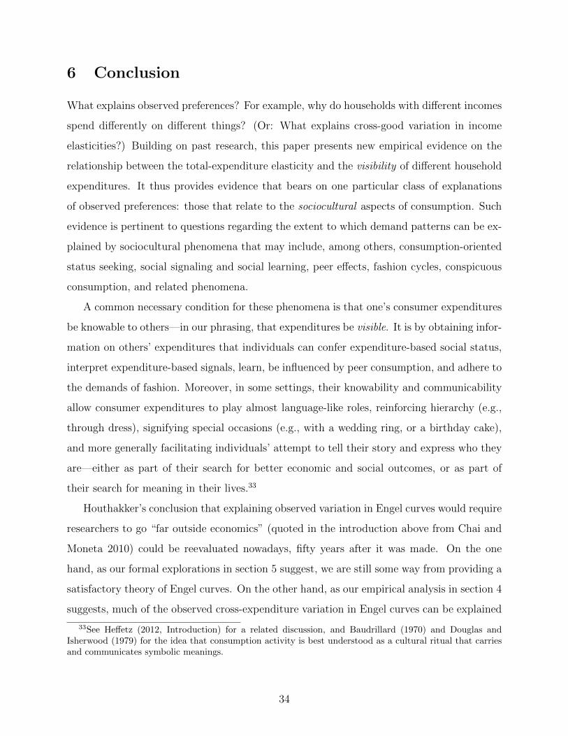
6 Conclusion

What explains observed preferences? For example, why do households with different incomes

spend differently on different things? (Or: What explains cross-good variation in income

elasticities?) Building on past research, this paper presents new empirical evidence on the

relationship between the total-expenditure elasticity and the visibility of different household

expenditures. It thus provides evidence that bears on one particular class of explanations

of observed preferences: those that relate to the sociocultural aspects of consumption. Such

evidence is pertinent to questions regarding the extent to which demand patterns can be ex-

plained by sociocultural phenomena that may include, among others, consumption-oriented

status seeking, social signaling and social learning, peer effects, fashion cycles, conspicuous

consumption, and related phenomena.

A common necessary condition for these phenomena is that one’s consumer expenditures

be knowable to others—in our phrasing, that expenditures be visible. It is by obtaining infor-

mation on others’ expenditures that individuals can confer expenditure-based social status,

interpret expenditure-based signals, learn, be influenced by peer consumption, and adhere to

the demands of fashion. Moreover, in some settings, their knowability and communicability

allow consumer expenditures to play almost language-like roles, reinforcing hierarchy (e.g.,

through dress), signifying special occasions (e.g., with a wedding ring, or a birthday cake),

and more generally facilitating individuals’ attempt to tell their story and express who they

are—either as part of their search for better economic and social outcomes, or as part of

their search for meaning in their lives.33

Houthakker’s conclusion that explaining observed variation in Engel curves would require

researchers to go “far outside economics” (quoted in the introduction above from Chai and

Moneta 2010) could be reevaluated nowadays, fifty years after it was made. On the one

hand, as our formal explorations in section 5 suggest, we are still some way from providing a

satisfactory theory of Engel curves. On the other hand, as our empirical analysis in section 4

suggests, much of the observed cross-expenditure variation in Engel curves can be explained

33See Heffetz (2012, Introduction) for a related discussion, and Baudrillard (1970) and Douglas andIsherwood (1979) for the idea that consumption activity is best understood as a cultural ritual that carriesand communicates symbolic meanings.

34

by (or explain) the difference between upward and downward sociocultural noticeability,

especially when combined with measures of impression quality.

More generally, expenditure visibility is a potentially important, yet mostly unexplored,

feature of consumer expenditures, that appears highly correlated with hitherto unexplained

variation in a range of consumer behaviors. The data presented in this paper confirm that it

is empirically measurable; show it to be remarkably stable across two decennial survey waves,

across interview modes, and across respondent samples; and, importantly, show that it is

multidimensional. Such evidence in turn suggests that one-off (or infrequent) online surveys

using a simple design and a relatively small convenience sample may be an inexpensive way

to generate highly applicable visibility data. In addition to the applications discussed in the

introduction, we would like to see the existing visibility data (surveyed in table 1) applied

in new domains. Moving beyond existing data, we would like to see new visibility data

collected: in new places; on new, finer consumption categories; and eliciting new, subtler

notions of visibility.

References

AAPOR (2016). Standard Definitions: Final Dispositions of Case Codes and Outcome Rates

for Surveys. 9th edition. The American Association for Public Opinion Research.

Baudrillard, Jean (1970). The Consumer Society: Myths & Structures. 1998 Edition, Sage

Publications, London.

Bellet, Clement, and Eve Sihra (2018). “The Conspicuous Consumption of the Poor: For-

going Calories for Aspirational Goods.” Working Paper.

Bertrand, Marianne and Adair Morse (2016). “Trickle-Down Consumption.” Review of

Economics and Statistics 98(5): 863–879.

Chai, Andreas, and Alessio Moneta (2010). “Retrospectives: Engel Curves.” Journal of

Economic Perspectives 24(1): 225–240.

Chao, Angela and Juliet B. Schor (1998). “Empirical tests of status consumption: Evidence

from women’s cosmetics.” Journal of Economic Psychology 19, 107–131.

35

Charles, Kerwin, Erik Hurst and Nikolai Roussanov (2009). “Conspicuous Consumption and

Race.” Quarterly Journal of Economics 124(2), 425–467.

Cosaert, Sam (2018). “Revealed Preferences for Diamond Goods.” American Economic

Journal: Microeconomics 10(2), 83–117.

De Giorgi, Giacomo, Anders Frederiksen, and Luigi Pistaferri (2016). “Consumption Net-

work Effects.” NBER Working Paper 22357.

Douglas, Mary and Baron Isherwood (1979). The World of Goods: Towards an Anthropology

of Consumption. New edition 1996, Routledge, London.

Fan, Jianqing (1992). “Design-adaptive nonparametric regression.” Journal of the American

Statistical Association 87: 998-1004.

Frank, Robert H. (1985). “The demand for unobservable and other nonpositional goods.”

American Economic Review 75(1): 101–116.

Friehe, Tim and Mario Mechtel (2014). “Conspicuous consumption and political regimes:

Evidence from East and West Germany.” European Economic Review 67: 62–81.

Harris, Ed, and John Sabelhaus (2005). “Consumer Expenditure Survey Family-Level Ex-

tracts.” http://www.nber.org/data/ces_cbo.html.

Heffetz, Ori (2011). “A Test of Conspicuous Consumption: Visibility and Income Elastici-

ties.” Review of Economics and Statistics, 93(4): 1101–1117.

Heffetz, Ori (2012). “Who Sees What? Demographics and the Visibility of Consumer Ex-

penditures.” Journal of Economic Psychology, 33(4): 801–817.

Hicks, Daniel L. and Joan Hamory Hicks (2014). “Jealous of the Joneses: conspicuous

consumption, inequality, and crime.” Oxford Economic Papers 66(4): 1090–1120.

Hillesheim, Inga and Mario Mechtel (2013). “How much do others matter? Explaining

positional concerns for different goods and personal characteristics.” Journal of Economic

Psychology 34: 61–77.

Ireland, Norman J. (1994). “On Limiting the Market for Status Signals.” Journal of Public

Economics 53(1): 91–110.

Jaikumar, Saravana, and Ankur Sarin (2015). “Conspicuous consumption and income in-

36

equality in an emerging economy: evidence from India.” Marketing Letters 26: 279–292.

Kamakura, Wagner A., and Rex Yuxing Du (2012). “How economic contractions and ex-

pansions affect expenditure patterns.” Journal of Consumer Research 39(2): 229–247.

Khamis, Melanie, Nishith Prakash, and Zahra Siddique (2012). “Consumption and social

identity: Evidence from India.” Journal of Economic Behavior & Organization 83(3):

353–371.

Maslow, Abraham H. (1943). “A Theory of Human Motivation.” Psychological Review

50(4): 370–396.

Mejıa, Daniel and Pascual Restrepo (2016). “Crime and conspicuous consumption.” Journal

of Public Economics 135: 1–14.

Ng, Yew-Kwang (1987). “Diamonds are a government’s best friend: burden-free taxes on

goods valued for their values.” American Economic Review 77(1): 186–191.

Veblen, Thorstein (1899). The Theory of the Leisure Class. Reprint 1965, MacMillan, New

York.

37

A Web Appendix

Expenditure Visibility and Consumer Behavior:

New Evidence

Ori Heffetz

October 7, 2018

A.1 Additional Survey-Design Detail: 31 Expenditure Categories

Construction of the original 31-category list for the 2004 survey was based on Harris and

Sabelhaus’s (2005) CEX extracts, as detailed in Heffetz (2004). In the decade from 2004 to

2014, household expenditure shares in the CEX decreased for some items—formally, universal

classification codes, or UCCs, of which there are several hundreds in the CEX—as increasing

shares were redirected toward newly available goods and services. While this transition from

older goods and services to newer substitutes affected expenditures on specific items/UCCs—

in some cases dramatically, as obsolete goods and services were entirely replaced by superior

alternatives—its effects on the 31-category list was limited. For example, while consumers

increasingly switch from printed to digital books and magazines, the original category Bks

(“Books, including school books, newspapers and magazines. . . ”) needed no modification.

After carefully reviewing the original list and comparing it with the most recently avail-

able data on consumer expenditures at the time of redesigning the survey (e.g., BLS, 2013),

we made slight modifications to only two of the 31 categories in the original list. Specifi-

cally, in the category Ot1 (Recreation 1) we replaced “video . . . equipment” with “visual

. . . equipment” and “tapes, CDs” with “music” (generalizing from specific, outdated tech-

nologies to broader categories); and we replaces “games” with “games, etc.” and moved

“games” from right after “computers” to right after “music” (viewing games more as exam-

ples of content—as is music—and less as examples of equipment—as are computers).1 And

1Replacing specific outdated technologies with more general categories, rather than with current tech-nologies, is intended also to minimize the potential need to update the list again in the future.

1

in the category Ot2 (Recreation 2) we added “internet” (and replaced “and” with “,”).2

In summary, our updated list of 31 consumption categories is identical to the original

2004 list in all but two categories (Ot1 and Ot2), which in turn saw only slight modifications.

Importantly, the two modified categories maintain the spirit of the original categories. For

example, they are not longer than the original categories, and they rely on familiar examples

rather than on more technical expressions (we avoided “information technology,” “commu-

nications devices,” etc.). That said, since modifying even a single word in a survey question

could potentially have great consequences, one should pay special attention to these two

categories when interpreting the data.

References A.1

BLS (2013). “Table 1 (2011-2012 Weights). Relative importance of components in the

Consumer Price Indexes: U.S. city average, December 2013.” https://www.bls.gov/

cpi/tables/relative-importance/2013.pdf.

Heffetz, Ori (2004). “Conspicuous Consumption and the Visibility of Consumer Expen-

ditures.” Working Paper, Princeton University. http://nber.org/~heffetz/papers/

conspicuous.pdf.

A.2 Additional CEX-Data Detail

The analysis of household expenditures in the original 2004 visibility-elasticity application

(Heffetz, 2011) was based on “10,400 households for which full-year expenditure data exist in

the 2003:3–2004:2 and 2005:1–2005:4 CEX extracts from Harris and Sabelhaus (2005).” As

documented in that paper, those CEX extracts, which surround the time during which the

2004 visibility survey was conducted, are not available online; they were kindly provided by

Ed Harris, though without documentation. The documentation and data that are publicly

2The addition of “internet” was motivated by the “Communication” category in the BLS (2013) table,where “Internet services and electronic information providers” account for 0.7% of expenditures. The locationof “internet” right after “Cable TV” reflects our intended interpretation of “internet” as referring to internetservices for the home (which are often purchased as a combined package with cable TV), rather than asmobile internet services. Relatedly, we hope that the category Cel (“mobile phone services,” unmodifiedfrom the original list) is perceived by respondents as including mobile internet services (which are oftenpurchased as a combined package with mobile call and text services).

2

available in Harris and Sabelhaus (2005) end in 2003:2.3

The updated 2014 application in the present paper requires creating from the raw CEX

data (available on the Bureau of Labor Statistics website, at https://www.bls.gov/cex/

pumd_data.htm#stata) new full-year CEX extracts that match the structure of the original

extracts. For this purpose, we created new programs, based on the Harris and Sabelhaus

original programs and documentation. The new programs include two main updates. The

first involves adding all the new UCCs that were added to the CEX after 2003—i.e., after

the last year that is still covered by the Harris and Sabelhaus (2005) documentation—and

assigning them to the 31 original expenditure categories. (The updated assignments, along

with all the new and updated programs and documentation we created, are included in our

data package.) With the updated UCCs, the new programs create 2012:2–2014:1 full-year

CEX extracts. These eight extracts cover all households who started reporting expenditures

in 2012:2–2014:1, and whose last interview was therefore conducted during 2013–2014 (since

households report expenditures in four consecutive quarterly interviews). The analysis in

the present paper (section 4) is based on the 9,026 households with full-year expenditure

data in these extracts.

Our second main update involves classifying the two (updated) clothing categories, Clo

and Und, into 17 new subcategories that are used in the 2015 online clothing-only visi-

bility survey. (See section 2.2 for details on this reclassification, table 3 for the list of 17

subcategories, and our data package for the assignment of UCCs into subcategories.)

References A.2

BLS (2016). “2015 Changes. Interview Survey and Diary Survey Consumer Expendi-

ture Public Use Microdata. August 30, 2016.” https://www.bls.gov/cex/pumd/2015/

changes.pdf.

3As noted in Heffetz (2011, footnote 16): “Notice that due to the BLS’s decennial sample frame rebasingin 2005, households that began the survey in 2004:3 and 2004:4 cannot be tracked for the entire year andhence are not included in our data.” Another sample redesign a decade later, in 2015, resulted in a similarissue: households whose participation in the CEX spanned the 2015 sample redesign (because they beganthe relevant four quarterly interviews in 2014:3 and 2014:4) could not be tracked for a full year (BLS, 2016).

3

A.3 Additional Tables and Graphs

Table A.1: 2014 Telephone Survey, Respondent Demographics

Visibility Survey Census Etc.a

Observationsb Value (SE) Value

Mean values:

Age 495 46.0 (0.8) 46.4Household sizec 498 2.9 (0.1) 2.6Children under 18 in household 498 0.7 (0.0) 0.6

Percent distribution:

Female 500 49.4 (2.2) 51.5Black 495 9.9 (1.3) 12.0Hispanic 499 8.8 (1.3) 14.2Married 497 48.5 (2.2) 51.4Employed 499 62.5 (2.2) 58.6

Education 496Elementary (0-8) 0.8 (0.4) 5.6High school (9-12) 22.6 (1.9) 37.8College (13-16) 53.6 (2.2) 47.5Graduate school (17 or more) 23.0 (1.9) 9.2

Total household income: 474Less than $20,000 12.7 (1.5) 19.9$20,000 to $40,000 17.3 (1.7) 21.7$40,000 to $60,000 13.5 (1.6) 16.8$60,000 to $100,000 24.5 (2.0) 21.2$100,000 or more 32.1 (2.1) 20.4

Region: 498Northeast 22.3 (1.9) 18.3Midwest 23.9 (1.9) 21.7South 37.1 (2.2) 37.0West 16.7 (1.7) 23.0

Sources: author’s visibility survey; 2010 American Community Survey, 2010 Census, and 2011 CurrentPopulation Survey.

aEntire-population estimates for Household size, Children under 18 in household, and Total householdincome; 18+-population estimates for all other variables; see appendix table A.4 for further detail.

bNumber of respondents reporting demographic characteristic (out of a total of 500 respondents).cTop-coded at 8 (in visibility survey).

4

Table A.2: 2014 Online Survey, Respondent Demographics

Visibility Survey Census Etc.a

Observationsb Value (SE) Value

Mean values:

Age 1076 47.2 (0.5) 46.4Household sizec 1075 2.7 (0.0) 2.6Children under 18 in household 1066 0.6 (0.0) 0.6

Percent distribution:

Female 1079 53.7 (1.5) 51.5Black 1079 9.1 (0.9) 12.0Hispanic 1077 21.9 (1.3) 14.2Married 1078 48.5 (1.5) 51.4Employed 1074 53.0 (1.5) 58.6

Education 1079Elementary (0-8) 0.0 (0.0) 5.6High school (9-12) 22.5 (1.3) 37.8College (13-16) 60.8 (1.5) 47.5Graduate school (17 or more) 16.7 (1.1) 9.2

Total household income: 1078Less than $20,000 16.9 (1.1) 19.9$20,000 to $40,000 24.8 (1.3) 21.7$40,000 to $60,000 18.7 (1.2) 16.8$60,000 to $100,000 22.9 (1.3) 21.2$100,000 or more 16.7 (1.1) 20.4

Region: 1052Northeast 18.9 (1.2) 18.3Midwest 20.1 (1.2) 21.7South 36.6 (1.5) 37.0West 24.4 (1.3) 23.0

Sources: author’s visibility survey; 2010 American Community Survey, 2010 Census, and 2011 CurrentPopulation Survey.

aEntire-population estimates for Household size, Children under 18 in household, and Total householdincome; 18+-population estimates for all other variables; see appendix table A.4 for further detail.

bNumber of respondents reporting demographic characteristic (out of a total of 1079 respondents).cTop-coded at 8 (in visibility survey).

5

Table A.3: 2015 Online Survey, Clothing, Respondent Demographics

Visibility Survey Census Etc.a

Observationsb Value (SE) Value

Mean values:

Age 1418 49.2 (0.4) 46.4Household sizec 1423 2.7 (0.0) 2.6Children under 18 in household 1412 0.6 (0.0) 0.6

Percent distribution:

Female 1425 51.4 (1.3) 51.5Black 1425 8.3 (0.7) 12.0Hispanic 1426 9.5 (0.8) 14.2Married 1425 63.0 (1.3) 51.4Employed 1424 59.6 (1.3) 58.6

Education 1425Elementary (0-8) 0.1 (0.1) 5.6High school (9-12) 17.1 (1.0) 37.8College (13-16) 58.2 (1.3) 47.5Graduate school (17 or more) 24.6 (1.1) 9.2

Total household income: 1424Less than $20,000 10.0 (0.8) 19.9$20,000 to $40,000 14.0 (0.9) 21.7$40,000 to $60,000 14.7 (0.9) 16.8$60,000 to $100,000 27.8 (1.2) 21.2$100,000 or more 33.4 (1.2) 20.4

Region: 1400Northeast 23.2 (1.1) 18.3Midwest 18.6 (1.0) 21.7South 35.4 (1.3) 37.0West 22.8 (1.1) 23.0

Sources: author’s visibility survey; 2010 American Community Survey, 2010 Census, and 2011 CurrentPopulation Survey.

aEntire-population estimates for Household size, Children under 18 in household, and Total householdincome; 18+-population estimates for all other variables; see appendix table A.4 for further detail.

bNumber of respondents reporting demographic characteristic (out of a total of 1426 respondents).cTop-coded at 8 (in visibility survey).

6

Table A.4: Data Source and Variable Construction for Census Etc Column in Tables A.1–A.3

Variable Tables Source Notes

Age Table PCT12: SEX BY AGE - Universe:Total population

2010 Census Sum-mary File 1

Calculated mean for 18years and over.

Householdsize

Table DP-1: Profile of General Populationand Housing Characteristics

2010 Census Sum-mary File 1

Given as the averagehousehold size.

Childrenunder 18 inhousehold

Table DP-1: Profile of General Populationand Housing Characteristics

2010 Census Sum-mary File 1

Including other rela-tive and non-relativechildren under 18.

Female Table DP-1: Profile of General Populationand Housing Characteristics

2010 Census Sum-mary File 1

Calculated for 18 yearsand over.

Black Table QT-PL: Race, Hispanic or Latino,Age, and Housing Occupancy: 2010

2010 Census Na-tional SummaryFile of Redistrict-ing Data

Calculated for 18 yearsand over.

Hispanic Table QT-PL: Race, Hispanic or Latino,Age, and Housing Occupancy: 2010

2010 Census Na-tional SummaryFile of Redistrict-ing Data

Calculated as Hispanicor Latino (of any race)for 18 years and over.

Married Table B12002: SEX BY MARITAL STA-TUS BY AGE FOR THE POPULATION15 YEARS AND OVER - Universe: Popu-lation 15 years and over

2010 Ameri-can CommunitySurvey 1-YearEstimates

Calculated as married,excluding separated,for 18 years and over.

Employed Table B01001: SEX BY AGE - Universe:Total population. Table B21005: AGE BYVETERAN STATUS BY EMPLOYMENTSTATUS FOR THE CIVILIAN POPU-LATION 18 TO 64 - Universe: Popula-tion 16 years and over. Table B23001:SEX BY AGE BY EMPLOYMENT STA-TUS FOR THE POPULATION 16 YEARSAND OVER - Universe: Population 16years and over

2010 Ameri-can CommunitySurvey 1-YearEstimates

Calculated percent em-ployed for 18 years andover.

Education Table B15001: SEX BY AGE BY EDUCA-TIONAL ATTAINMENT FOR THE POP-ULATION 18 YEARS AND OVER - Uni-verse: Population 18 years and over

2010 Ameri-can CommunitySurvey 1-YearEstimates

Calculated distribu-tion for 18 years andover.

Totalhouseholdincome

Table HINC-06: Income Distribution to$250,000 or More for Households: 2010

Current Popula-tion Survey, 2011Annual Socialand EconomicSupplement

Total household in-come.

Region Table PCT12: SEX BY AGE - Universe:Total population

2010 Census Sum-mary File 1

Chose geographic unitsas regions. Calculatedfor 18 years and over.

7

Table A.5: 2014 Telephone Survey, Notice More (NM) Scores and Rankings

Expenditure Category Avg. Coded Response Top Two Responses Top Three Responses

Score (SE) [Rank] Frac. (SE) [Rank] Frac. (SE) [Rank]

Car (cars) 0.72 (0.01) [ 1] 0.69 (0.02) [ 1] 0.83 (0.02) [ 1]Cig (cigarettes) 0.68 (0.02) [ 2] 0.67 (0.02) [ 2] 0.78 (0.02) [ 3]Clo (clothing) 0.66 (0.02) [ 3] 0.63 (0.02) [ 3] 0.79 (0.02) [ 2]Jwl (jewelry) 0.63 (0.02) [ 4] 0.60 (0.02) [ 4] 0.75 (0.02) [ 5]Ot1 (recreation 1) 0.62 (0.01) [ 5] 0.56 (0.02) [ 5] 0.77 (0.02) [ 4]Fur (furniture) 0.59 (0.01) [ 6] 0.50 (0.02) [ 7] 0.73 (0.02) [ 7]FdO (food out) 0.57 (0.01) [ 7] 0.51 (0.02) [ 6] 0.75 (0.02) [ 6]AlO (alcohol out) 0.56 (0.02) [ 8] 0.49 (0.02) [ 8] 0.70 (0.02) [ 9]Ot2 (recreation 2) 0.56 (0.01) [ 9] 0.47 (0.02) [10] 0.72 (0.02) [ 8]AlH (alcohol home) 0.55 (0.02) [10] 0.48 (0.02) [ 9] 0.68 (0.02) [10]Brb (barbers etc) 0.53 (0.02) [11] 0.45 (0.02) [11] 0.65 (0.02) [13]Edu (education) 0.52 (0.01) [12] 0.43 (0.02) [12] 0.65 (0.02) [12]Bks (books etc) 0.50 (0.01) [13] 0.40 (0.02) [13] 0.67 (0.02) [11]FdH (food home) 0.49 (0.01) [14] 0.37 (0.02) [16] 0.64 (0.02) [14]Hom (rent/home) 0.48 (0.02) [15] 0.40 (0.02) [14] 0.57 (0.02) [16]Cel (cell phone) 0.46 (0.02) [16] 0.40 (0.02) [15] 0.56 (0.02) [17]Htl (hotels etc) 0.45 (0.01) [17] 0.34 (0.02) [18] 0.60 (0.02) [15]Bus (public trans.) 0.44 (0.02) [18] 0.35 (0.02) [17] 0.53 (0.02) [18]CMn (car repair) 0.42 (0.01) [19] 0.30 (0.02) [20] 0.52 (0.02) [20]Air (air travel) 0.41 (0.02) [20] 0.30 (0.02) [21] 0.52 (0.02) [19]Gas (gasoline) 0.40 (0.02) [21] 0.31 (0.02) [19] 0.48 (0.02) [21]Med (health care) 0.38 (0.01) [22] 0.25 (0.02) [22] 0.46 (0.02) [22]Utl (home utilities) 0.34 (0.02) [23] 0.24 (0.02) [23] 0.41 (0.02) [23]Lry (laundry) 0.33 (0.02) [24] 0.24 (0.02) [24] 0.38 (0.02) [24]Tel (home phone) 0.31 (0.02) [25] 0.21 (0.02) [25] 0.37 (0.02) [25]Cha (charities) 0.30 (0.01) [26] 0.20 (0.02) [26] 0.36 (0.02) [26]CIn (car insur.) 0.27 (0.01) [27] 0.17 (0.02) [27] 0.32 (0.02) [27]Fee (legal fees) 0.25 (0.01) [28] 0.13 (0.01) [28] 0.27 (0.02) [28]HIn (home insur.) 0.20 (0.01) [29] 0.11 (0.01) [29] 0.21 (0.02) [29]LIn (life insur.) 0.17 (0.01) [30] 0.10 (0.01) [30] 0.18 (0.02) [30]Und (underwear) 0.16 (0.01) [31] 0.09 (0.01) [31] 0.16 (0.02) [31]

Source: author’s visibility survey (500 respondents).

8

Table A.6: 2014 Online Survey, Notice More (NM) Measures and Rankings

Expenditure Category Avg. Coded Response Top Two Responses Top Three Responses

Score (SE) [Rank] Frac. (SE) [Rank] Frac. (SE) [Rank]

Car (cars) 0.64 (0.02) [ 1] 0.61 (0.03) [ 1] 0.83 (0.02) [ 1]Cig (cigarettes) 0.62 (0.02) [ 2] 0.58 (0.03) [ 3] 0.76 (0.03) [ 4]Jwl (jewelry) 0.62 (0.02) [ 3] 0.59 (0.03) [ 2] 0.77 (0.03) [ 2]Fur (furniture) 0.60 (0.02) [ 4] 0.52 (0.03) [ 5] 0.75 (0.03) [ 5]Clo (clothing) 0.59 (0.02) [ 5] 0.52 (0.03) [ 4] 0.74 (0.03) [ 6]Ot1 (recreation 1) 0.57 (0.02) [ 6] 0.47 (0.03) [ 6] 0.77 (0.03) [ 3]AlO (alcohol out) 0.52 (0.02) [ 7] 0.41 (0.03) [ 9] 0.70 (0.03) [ 7]AlH (alcohol home) 0.52 (0.02) [ 8] 0.41 (0.03) [ 8] 0.68 (0.03) [ 9]FdO (food out) 0.52 (0.02) [ 9] 0.42 (0.03) [ 7] 0.69 (0.03) [ 8]Brb (barbers etc) 0.50 (0.02) [10] 0.39 (0.03) [10] 0.67 (0.03) [10]Ot2 (recreation 2) 0.49 (0.02) [11] 0.36 (0.03) [11] 0.64 (0.03) [11]FdH (food home) 0.45 (0.02) [12] 0.30 (0.03) [14] 0.63 (0.03) [12]Bks (books etc) 0.44 (0.02) [13] 0.31 (0.03) [12] 0.58 (0.03) [14]Htl (hotels etc) 0.44 (0.02) [14] 0.29 (0.03) [16] 0.58 (0.03) [13]Air (air travel) 0.43 (0.02) [15] 0.31 (0.03) [13] 0.57 (0.03) [15]Bus (public trans.) 0.42 (0.02) [16] 0.30 (0.03) [15] 0.56 (0.03) [17]Edu (education) 0.40 (0.02) [17] 0.24 (0.03) [20] 0.56 (0.03) [16]Cel (cell phone) 0.39 (0.02) [18] 0.26 (0.03) [18] 0.52 (0.03) [18]CMn (car repair) 0.39 (0.02) [19] 0.25 (0.03) [19] 0.49 (0.03) [19]Hom (rent/home) 0.37 (0.02) [20] 0.27 (0.03) [17] 0.46 (0.03) [20]Med (health care) 0.34 (0.02) [21] 0.19 (0.02) [24] 0.42 (0.03) [21]Gas (gasoline) 0.33 (0.02) [22] 0.20 (0.02) [23] 0.41 (0.03) [22]Tel (home phone) 0.32 (0.02) [23] 0.23 (0.03) [21] 0.40 (0.03) [23]Cha (charities) 0.32 (0.02) [24] 0.21 (0.02) [22] 0.40 (0.03) [25]Lry (laundry) 0.30 (0.02) [25] 0.17 (0.02) [26] 0.40 (0.03) [24]Utl (home utilities) 0.29 (0.02) [26] 0.18 (0.02) [25] 0.35 (0.03) [26]CIn (car insur.) 0.25 (0.02) [27] 0.16 (0.02) [27] 0.30 (0.03) [27]Fee (legal fees) 0.25 (0.02) [28] 0.14 (0.02) [29] 0.29 (0.03) [28]HIn (home insur.) 0.22 (0.02) [29] 0.13 (0.02) [31] 0.25 (0.03) [29]LIn (life insur.) 0.21 (0.02) [30] 0.14 (0.02) [28] 0.24 (0.03) [30]Und (underwear) 0.19 (0.02) [31] 0.14 (0.02) [30] 0.21 (0.02) [31]

Source: author’s visibility survey (277 respondents).

9

Table A.7: 2014 Online Survey, Notice Less (NL) Measures and Rankings

Expenditure Category Avg. Coded Response Top Two Responses Top Three Responses

Score (SE) [Rank] Frac. (SE) [Rank] Frac. (SE) [Rank]

Fur (furniture) 0.55 (0.02) [ 1] 0.46 (0.03) [ 2] 0.68 (0.03) [ 1]Cig (cigarettes) 0.52 (0.02) [ 2] 0.51 (0.03) [ 1] 0.61 (0.03) [ 5]Ot1 (recreation 1) 0.50 (0.02) [ 3] 0.39 (0.03) [ 4] 0.63 (0.03) [ 3]Clo (clothing) 0.49 (0.02) [ 4] 0.41 (0.03) [ 3] 0.63 (0.03) [ 2]Car (cars) 0.49 (0.02) [ 5] 0.35 (0.03) [ 7] 0.62 (0.03) [ 4]AlH (alcohol home) 0.45 (0.02) [ 6] 0.38 (0.03) [ 5] 0.57 (0.03) [ 8]FdO (food out) 0.45 (0.02) [ 7] 0.36 (0.03) [ 6] 0.60 (0.03) [ 6]Brb (barbers etc) 0.43 (0.02) [ 8] 0.31 (0.03) [12] 0.57 (0.03) [ 7]Ot2 (recreation 2) 0.43 (0.02) [ 9] 0.31 (0.03) [11] 0.56 (0.03) [ 9]Jwl (jewelry) 0.42 (0.02) [10] 0.34 (0.03) [ 8] 0.52 (0.03) [12]FdH (food home) 0.42 (0.02) [11] 0.29 (0.03) [13] 0.56 (0.03) [10]AlO (alcohol out) 0.42 (0.02) [12] 0.32 (0.03) [10] 0.56 (0.03) [11]Cel (cell phone) 0.40 (0.02) [13] 0.32 (0.03) [ 9] 0.51 (0.03) [13]CMn (car repair) 0.38 (0.02) [14] 0.25 (0.03) [20] 0.49 (0.03) [14]Hom (rent/home) 0.38 (0.02) [15] 0.28 (0.03) [14] 0.47 (0.03) [16]Bks (books etc) 0.38 (0.02) [16] 0.26 (0.03) [17] 0.48 (0.03) [15]Lry (laundry) 0.36 (0.02) [17] 0.27 (0.03) [15] 0.46 (0.03) [17]Bus (public trans.) 0.36 (0.02) [18] 0.27 (0.03) [16] 0.46 (0.03) [18]Edu (education) 0.34 (0.02) [19] 0.19 (0.02) [23] 0.43 (0.03) [20]Gas (gasoline) 0.34 (0.02) [20] 0.26 (0.03) [18] 0.44 (0.03) [19]Utl (home utilities) 0.33 (0.02) [21] 0.25 (0.03) [19] 0.41 (0.03) [21]Htl (hotels etc) 0.32 (0.02) [22] 0.18 (0.02) [25] 0.38 (0.03) [23]Tel (home phone) 0.32 (0.02) [23] 0.21 (0.03) [21] 0.41 (0.03) [22]Med (health care) 0.31 (0.02) [24] 0.19 (0.02) [24] 0.38 (0.03) [24]Air (air travel) 0.30 (0.02) [25] 0.16 (0.02) [27] 0.36 (0.03) [25]Cha (charities) 0.26 (0.02) [26] 0.19 (0.02) [22] 0.29 (0.03) [27]CIn (car insur.) 0.26 (0.02) [27] 0.17 (0.02) [26] 0.30 (0.03) [26]HIn (home insur.) 0.22 (0.02) [28] 0.13 (0.02) [30] 0.25 (0.03) [28]Fee (legal fees) 0.21 (0.02) [29] 0.14 (0.02) [28] 0.24 (0.03) [29]Und (underwear) 0.20 (0.02) [30] 0.13 (0.02) [29] 0.22 (0.03) [30]LIn (life insur.) 0.19 (0.02) [31] 0.12 (0.02) [31] 0.22 (0.03) [31]

Source: author’s visibility survey (263 respondents).

10

Table A.8: 2014 Online Survey, Impression More (IM) Measures and Rankings

Expenditure Category Avg. Coded Response Top Two Responses Top Three Responses

Score (SE) [Rank] Frac. (SE) [Rank] Frac. (SE) [Rank]

Cha (charities) 0.64 (0.01) [ 1] 0.47 (0.03) [ 1] 0.94 (0.01) [ 8]Edu (education) 0.64 (0.01) [ 2] 0.46 (0.03) [ 2] 0.96 (0.01) [ 1]Bks (books etc) 0.60 (0.01) [ 3] 0.38 (0.03) [ 3] 0.95 (0.01) [ 6]LIn (life insur.) 0.59 (0.01) [ 4] 0.33 (0.03) [ 4] 0.96 (0.01) [ 2]HIn (home insur.) 0.57 (0.01) [ 5] 0.27 (0.03) [ 6] 0.95 (0.01) [ 4]Med (health care) 0.57 (0.01) [ 6] 0.25 (0.03) [ 8] 0.95 (0.01) [ 3]CMn (car repair) 0.57 (0.01) [ 7] 0.27 (0.03) [ 7] 0.95 (0.01) [ 5]CIn (car insur.) 0.56 (0.01) [ 8] 0.24 (0.03) [12] 0.94 (0.01) [ 9]Bus (public trans.) 0.56 (0.01) [ 9] 0.25 (0.03) [10] 0.94 (0.01) [10]Fur (furniture) 0.56 (0.01) [10] 0.25 (0.03) [ 9] 0.93 (0.02) [11]Ot1 (recreation 1) 0.55 (0.01) [11] 0.28 (0.03) [ 5] 0.87 (0.02) [21]Htl (hotels etc) 0.55 (0.01) [12] 0.24 (0.03) [11] 0.91 (0.02) [15]Hom (rent/home) 0.54 (0.01) [13] 0.19 (0.02) [17] 0.92 (0.02) [13]Und (underwear) 0.54 (0.01) [14] 0.16 (0.02) [25] 0.94 (0.01) [ 7]FdH (food home) 0.54 (0.01) [15] 0.18 (0.02) [21] 0.92 (0.02) [12]Clo (clothing) 0.53 (0.01) [16] 0.20 (0.02) [15] 0.88 (0.02) [19]Fee (legal fees) 0.53 (0.01) [17] 0.18 (0.02) [22] 0.92 (0.02) [14]Ot2 (recreation 2) 0.53 (0.01) [18] 0.20 (0.02) [16] 0.86 (0.02) [23]Lry (laundry) 0.53 (0.01) [19] 0.19 (0.02) [20] 0.90 (0.02) [16]Car (cars) 0.53 (0.01) [20] 0.21 (0.02) [14] 0.87 (0.02) [22]Air (air travel) 0.52 (0.01) [21] 0.17 (0.02) [23] 0.88 (0.02) [20]Brb (barbers etc) 0.52 (0.01) [22] 0.23 (0.03) [13] 0.83 (0.02) [26]Tel (home phone) 0.52 (0.01) [23] 0.15 (0.02) [26] 0.89 (0.02) [18]Gas (gasoline) 0.52 (0.01) [24] 0.14 (0.02) [27] 0.89 (0.02) [17]Utl (home utilities) 0.51 (0.01) [25] 0.16 (0.02) [24] 0.86 (0.02) [24]FdO (food out) 0.51 (0.01) [26] 0.19 (0.02) [18] 0.82 (0.02) [27]Jwl (jewelry) 0.51 (0.01) [27] 0.19 (0.02) [19] 0.81 (0.02) [28]Cel (cell phone) 0.50 (0.01) [28] 0.14 (0.02) [29] 0.84 (0.02) [25]AlO (alcohol out) 0.44 (0.01) [29] 0.14 (0.02) [28] 0.68 (0.03) [29]AlH (alcohol home) 0.42 (0.01) [30] 0.12 (0.02) [30] 0.64 (0.03) [30]Cig (cigarettes) 0.34 (0.02) [31] 0.09 (0.02) [31] 0.51 (0.03) [31]

Source: author’s visibility survey (272 respondents).

11

Table A.9: 2014 Online Survey, Impression Less (IL) Measures and Rankings

Expenditure Category Avg. Coded Response Top Two Responses Top Three Responses

Score (SE) [Rank] Frac. (SE) [Rank] Frac. (SE) [Rank]

Cig (cigarettes) 0.65 (0.02) [ 1] 0.46 (0.03) [ 1] 0.88 (0.02) [23]AlH (alcohol home) 0.65 (0.01) [ 2] 0.45 (0.03) [ 2] 0.94 (0.01) [12]AlO (alcohol out) 0.63 (0.01) [ 3] 0.42 (0.03) [ 3] 0.94 (0.01) [11]Hom (rent/home) 0.62 (0.01) [ 4] 0.37 (0.03) [ 6] 0.96 (0.01) [ 3]Cel (cell phone) 0.62 (0.01) [ 5] 0.38 (0.03) [ 5] 0.95 (0.01) [ 6]Ot2 (recreation 2) 0.61 (0.01) [ 6] 0.40 (0.03) [ 4] 0.92 (0.02) [16]FdO (food out) 0.61 (0.01) [ 7] 0.37 (0.03) [ 9] 0.95 (0.01) [ 9]Ot1 (recreation 1) 0.61 (0.01) [ 8] 0.36 (0.03) [10] 0.96 (0.01) [ 2]Jwl (jewelry) 0.61 (0.01) [ 9] 0.34 (0.03) [12] 0.95 (0.01) [ 7]Car (cars) 0.61 (0.01) [10] 0.37 (0.03) [ 7] 0.94 (0.01) [10]Gas (gasoline) 0.61 (0.01) [11] 0.35 (0.03) [11] 0.95 (0.01) [ 8]Tel (home phone) 0.61 (0.01) [12] 0.33 (0.03) [13] 0.96 (0.01) [ 1]Air (air travel) 0.60 (0.01) [13] 0.33 (0.03) [14] 0.96 (0.01) [ 5]Utl (home utilities) 0.60 (0.01) [14] 0.37 (0.03) [ 8] 0.90 (0.02) [19]Brb (barbers etc) 0.59 (0.01) [15] 0.31 (0.03) [15] 0.93 (0.02) [15]FdH (food home) 0.59 (0.01) [16] 0.31 (0.03) [17] 0.92 (0.02) [17]Fur (furniture) 0.59 (0.01) [17] 0.31 (0.03) [16] 0.94 (0.01) [13]Bus (public trans.) 0.58 (0.01) [18] 0.28 (0.03) [22] 0.96 (0.01) [ 4]Htl (hotels etc) 0.58 (0.01) [19] 0.29 (0.03) [18] 0.93 (0.02) [14]Fee (legal fees) 0.57 (0.01) [20] 0.25 (0.03) [26] 0.92 (0.02) [18]Clo (clothing) 0.56 (0.01) [21] 0.28 (0.03) [20] 0.89 (0.02) [21]CMn (car repair) 0.56 (0.01) [22] 0.28 (0.03) [21] 0.83 (0.02) [29]LIn (life insur.) 0.55 (0.01) [23] 0.25 (0.03) [25] 0.90 (0.02) [20]CIn (car insur.) 0.55 (0.01) [24] 0.28 (0.03) [19] 0.87 (0.02) [25]Lry (laundry) 0.55 (0.01) [25] 0.26 (0.03) [23] 0.87 (0.02) [24]Bks (books etc) 0.54 (0.01) [26] 0.24 (0.03) [28] 0.87 (0.02) [26]Und (underwear) 0.54 (0.01) [27] 0.21 (0.02) [31] 0.88 (0.02) [22]Med (health care) 0.53 (0.01) [28] 0.25 (0.03) [24] 0.80 (0.02) [31]Cha (charities) 0.53 (0.01) [29] 0.22 (0.03) [30] 0.84 (0.02) [28]HIn (home insur.) 0.53 (0.01) [30] 0.23 (0.03) [29] 0.84 (0.02) [27]Edu (education) 0.53 (0.01) [31] 0.25 (0.03) [27] 0.81 (0.02) [30]

Source: author’s visibility survey (267 respondents).

12

Table A.10: 2015 Online Survey, Clothing, Notice More (NM) Measures and Rankings

Expenditure Category Avg. Coded Response Top Two Responses Top Three Responses

Score (SE) [Rank] Frac. (SE) [Rank] Frac. (SE) [Rank]

Owr (outerwear) 0.55 (0.01) [ 1] 0.44 (0.02) [ 2] 0.69 (0.02) [ 1]Wmn (women) 0.54 (0.01) [ 2] 0.46 (0.02) [ 1] 0.68 (0.02) [ 2]Sts (suits etc) 0.53 (0.01) [ 3] 0.44 (0.02) [ 3] 0.66 (0.02) [ 3]Men (men) 0.50 (0.01) [ 4] 0.38 (0.02) [ 6] 0.64 (0.02) [ 4]ShW (women’s shoes) 0.49 (0.01) [ 5] 0.38 (0.02) [ 5] 0.64 (0.02) [ 5]Acc (accessories) 0.48 (0.01) [ 6] 0.39 (0.02) [ 4] 0.60 (0.02) [ 6]Grl (girls) 0.45 (0.01) [ 7] 0.35 (0.02) [ 7] 0.59 (0.02) [ 7]Spo (sports) 0.44 (0.01) [ 8] 0.32 (0.02) [ 9] 0.57 (0.02) [ 8]Boy (boys) 0.41 (0.01) [ 9] 0.29 (0.02) [10] 0.53 (0.02) [ 9]ShM (men’s shoes) 0.41 (0.01) [10] 0.32 (0.02) [ 8] 0.51 (0.02) [10]ShG (girls’ shoes) 0.38 (0.01) [11] 0.29 (0.02) [11] 0.49 (0.02) [12]Inf (infants) 0.37 (0.01) [12] 0.28 (0.02) [12] 0.49 (0.02) [11]ShB (boys’ shoes) 0.37 (0.01) [13] 0.26 (0.02) [13] 0.48 (0.02) [13]Oth (luggage etc) 0.34 (0.01) [14] 0.25 (0.02) [14] 0.40 (0.02) [14]Soc (socks) 0.22 (0.01) [15] 0.14 (0.01) [16] 0.26 (0.02) [15]Nwr (nightwear) 0.20 (0.01) [16] 0.15 (0.01) [15] 0.22 (0.02) [16]Uwr (underwear) 0.15 (0.01) [17] 0.11 (0.01) [17] 0.18 (0.01) [17]

Source: author’s visibility survey (713 respondents).

Table A.11: 2015 Online Survey, Clothing, Notice Less (NL) Measures and Rankings

Expenditure Category Avg. Coded Response Top Two Responses Top Three Responses

Score (SE) [Rank] Frac. (SE) [Rank] Frac. (SE) [Rank]

Wmn (women) 0.43 (0.01) [ 1] 0.33 (0.02) [ 1] 0.55 (0.02) [ 1]Men (men) 0.41 (0.01) [ 2] 0.30 (0.02) [ 2] 0.52 (0.02) [ 2]Sts (suits etc) 0.41 (0.01) [ 3] 0.30 (0.02) [ 3] 0.50 (0.02) [ 3]Owr (outerwear) 0.40 (0.01) [ 4] 0.28 (0.02) [ 4] 0.50 (0.02) [ 4]Grl (girls) 0.38 (0.01) [ 5] 0.28 (0.02) [ 5] 0.49 (0.02) [ 5]ShW (women’s shoes) 0.37 (0.01) [ 6] 0.28 (0.02) [ 6] 0.46 (0.02) [ 6]Boy (boys) 0.37 (0.01) [ 7] 0.27 (0.02) [ 7] 0.45 (0.02) [ 7]ShM (men’s shoes) 0.34 (0.01) [ 8] 0.24 (0.02) [11] 0.41 (0.02) [10]Inf (infants) 0.34 (0.01) [ 9] 0.25 (0.02) [ 8] 0.42 (0.02) [ 8]ShG (girls’ shoes) 0.33 (0.01) [10] 0.24 (0.02) [ 9] 0.40 (0.02) [12]Spo (sports) 0.33 (0.01) [11] 0.20 (0.02) [13] 0.42 (0.02) [ 9]Acc (accessories) 0.33 (0.01) [12] 0.21 (0.02) [12] 0.40 (0.02) [11]ShB (boys’ shoes) 0.32 (0.01) [13] 0.24 (0.02) [10] 0.39 (0.02) [13]Oth (luggage etc) 0.24 (0.01) [14] 0.17 (0.02) [14] 0.26 (0.02) [14]Soc (socks) 0.20 (0.01) [15] 0.14 (0.01) [15] 0.23 (0.02) [15]Nwr (nightwear) 0.19 (0.01) [16] 0.14 (0.01) [16] 0.22 (0.02) [16]Uwr (underwear) 0.15 (0.01) [17] 0.12 (0.01) [17] 0.18 (0.01) [17]

Source: author’s visibility survey (713 respondents).

13

Table A.12: Average Total-Expenditure Elasticity: All Households & by Quintile (31 Cat.)

All Q1 Q2 Q3 Q4 Q5

FdH (food home) 0.53 0.54 0.57 0.56 0.50 0.47FdO (food out) 1.16 1.30 1.27 1.17 1.05 1.03Cig (cigarettes) −0.02 0.37 0.10 0.18 −0.20 −0.60AlH (alcohol home) 0.99 0.68 0.99 1.28 1.08 0.88AlO (alcohol out) 1.42 1.21 1.54 1.66 1.38 1.26Clo (clothing) 1.21 1.26 1.25 1.33 1.19 1.01Und (underwear etc.) 1.06 0.79 1.16 1.19 1.20 0.90Lry (laundry) 0.60 −0.15 −0.05 0.51 1.17 1.55Jwl (jewelry) 1.99 1.52 1.90 2.61 2.14 1.65Brb (barbers etc.) 1.30 1.38 1.58 1.29 1.24 0.98Hom (rent/home) 0.82 1.00 0.89 0.77 0.72 0.75Htl (hotels etc.) 2.27 2.39 2.38 2.29 2.36 1.89Fur (furniture) 1.45 1.23 1.84 1.64 1.42 1.08Utl (home utilities) 0.55 0.85 0.57 0.49 0.40 0.47Tel (home telephone) 0.51 0.67 0.56 0.49 0.30 0.52Cel (cell phone) 0.78 1.01 1.03 0.90 0.54 0.37HIn (home insurance) 1.59 2.05 1.76 1.34 1.34 1.48Med (health care) 1.08 1.31 1.26 1.12 0.93 0.77Fee (legal fees) 1.06 1.26 1.21 0.99 1.03 0.80LIn (life insur.) 1.52 0.98 1.52 1.72 1.80 1.53Car (cars) 2.67 2.65 2.86 3.23 2.73 1.77CMn (car repair) 1.33 1.63 1.58 1.36 1.14 0.89Gas (gasoline) 0.83 1.36 1.02 0.84 0.54 0.37Cin (car insur.) 0.93 1.53 1.08 0.78 0.69 0.59Bus (public trans.) 0.93 −0.09 0.34 1.00 1.66 1.73Air (air travel) 2.00 1.96 2.29 1.94 1.96 1.85Bks (books etc.) 1.29 1.10 1.21 1.55 1.35 1.20Ot1 (recreation 1) 1.51 1.52 1.54 1.61 1.63 1.24Ot2 (recreation 2) 1.11 0.99 1.10 1.11 1.19 1.17Edu (education) 2.17 1.45 1.67 2.86 2.58 2.18Cha (charities) 1.58 1.63 1.69 1.53 1.53 1.49

Notes: Average total-expenditure elasticity, for all households and by total-expenditure quintile (31 cate-gories). Estimated from 2012:2–2014:1 full-year CEX extracts.

14

Table A.13: Average Expenditure Shares (percent): All Households & by Quintile (31 Cat.)

All Q1 Q2 Q3 Q4 Q5

FdH (food home) 12.68 18.34 14.02 12.13 10.52 8.08FdO (food out) 4.62 3.78 4.53 4.77 5.04 5.02Cig (cigarettes) 0.92 1.68 1.09 0.84 0.64 0.30AlH (alcohol home) 0.44 0.48 0.40 0.42 0.49 0.43AlO (alcohol out) 0.27 0.19 0.21 0.27 0.33 0.36Clo (clothing) 1.65 1.37 1.46 1.71 1.85 1.89Und (underwear etc.) 0.11 0.11 0.09 0.11 0.11 0.11Lry (laundry) 0.22 0.42 0.21 0.15 0.15 0.19Jwl (jewelry) 0.13 0.05 0.08 0.10 0.19 0.26Brb (barbers etc.) 0.55 0.37 0.50 0.59 0.63 0.66Hom (rent/home) 31.42 34.79 34.17 32.45 29.38 25.93Htl (hotels etc.) 0.61 0.13 0.34 0.47 0.78 1.37Fur (furniture) 1.52 0.91 1.24 1.56 1.86 2.09Utl (home utilities) 6.00 8.10 6.96 6.03 5.01 3.75Tel (home telephone) 1.00 1.44 1.13 1.00 0.81 0.59Cel (cell phone) 2.08 2.21 2.27 2.28 2.06 1.56HIn (home insurance) 1.57 0.82 1.36 1.70 1.75 2.28Med (health care) 7.81 6.53 7.85 8.39 8.49 7.82Fee (legal fees) 1.38 1.22 1.43 1.45 1.43 1.38LIn (life insur.) 0.61 0.39 0.42 0.57 0.69 1.01Car (cars) 4.40 0.65 1.46 2.98 6.32 11.06CMn (car repair) 1.79 1.18 1.68 1.93 2.13 2.07Gas (gasoline) 6.02 5.97 6.83 6.71 5.97 4.53Cin (car insur.) 1.98 1.79 2.33 2.17 1.98 1.64Bus (public trans.) 0.38 0.59 0.28 0.28 0.30 0.48Air (air travel) 0.54 0.17 0.36 0.48 0.65 1.08Bks (books etc.) 0.54 0.44 0.45 0.50 0.63 0.69Ot1 (recreation 1) 1.11 0.67 0.84 1.12 1.29 1.68Ot2 (recreation 2) 3.51 3.27 3.34 3.43 3.58 3.99Edu (education) 1.51 0.52 0.63 0.88 1.97 3.71Cha (charities) 2.58 1.42 2.04 2.54 2.98 3.98

Total 100.00 100.00 100.00 100.00 100.00 100.00

Notes: Average expenditure shares (%), for all households and by total-expenditure quintile (31 categories).Calculated from 2012:2–2014:1 full-year CEX extracts.

15

Table A.14: Average Total-Expenditure Elasticity: All Households & by Quintile (17 Sub.)

All Q1 Q2 Q3 Q4 Q5

Acc (accessories) 1.43 1.75 1.20 1.47 1.58 1.17Sts (suits etc.) 1.62 1.08 1.70 2.03 1.76 1.42Boy (boys) 1.09 1.67 1.11 1.06 0.91 0.73Grl (girls) 1.29 1.69 1.45 1.29 1.16 0.88Men (men) 1.18 0.99 1.26 1.36 1.25 1.01Wmn (women) 1.28 1.32 1.36 1.31 1.23 1.14Inf (infants) 0.88 1.52 1.18 0.83 0.50 0.34Nwr (nightwear) 1.15 1.08 1.33 1.23 1.09 0.99Oth (luggage etc.) 1.39 1.31 1.25 1.54 1.63 1.20Owr (outerwear) 1.23 1.00 1.33 1.37 1.30 1.12ShB (boys’ shoes) 1.08 1.94 1.04 0.99 0.81 0.67ShG (girls’ shoes) 1.19 1.78 1.28 1.10 0.95 0.88ShM (men’s shoes) 1.05 0.87 1.00 1.30 1.17 0.85ShW (women’s shoes) 1.11 1.08 1.14 1.18 1.13 1.00Soc (socks) 1.06 0.74 1.16 1.28 1.18 0.87Spo (sports) 1.40 1.03 1.50 1.65 1.53 1.25Uwr (underwear) 0.99 0.68 1.02 1.14 1.16 0.93

Notes: Average total-expenditure elasticity, for all households and by total-expenditure quintile (17 clothing-only subcategories). Estimated from 2012:2–2014:1 full-year CEX extracts.

Table A.15: Average Expenditure Shares (percent): All Households & by Quintile (17 Sub.)

All Q1 Q2 Q3 Q4 Q5

Acc (accessories) 0.05 0.04 0.04 0.05 0.06 0.08Sts (suits etc.) 0.05 0.03 0.03 0.05 0.07 0.09Boy (boys) 0.10 0.09 0.10 0.11 0.11 0.10Grl (girls) 0.11 0.07 0.10 0.11 0.13 0.12Men (men) 0.26 0.23 0.23 0.26 0.30 0.30Wmn (women) 0.44 0.34 0.38 0.47 0.48 0.54Inf (infants) 0.12 0.10 0.14 0.14 0.12 0.08Nwr (nightwear) 0.03 0.03 0.02 0.03 0.03 0.03Oth (luggage etc.) 0.03 0.03 0.03 0.03 0.04 0.05Owr (outerwear) 0.10 0.08 0.08 0.10 0.10 0.12ShB (boys’ shoes) 0.04 0.04 0.04 0.05 0.04 0.04ShG (girls’ shoes) 0.03 0.03 0.03 0.04 0.04 0.03ShM (men’s shoes) 0.12 0.12 0.10 0.11 0.13 0.12ShW (women’s shoes) 0.14 0.14 0.13 0.15 0.15 0.16Soc (socks) 0.02 0.02 0.02 0.02 0.02 0.02Spo (sports) 0.05 0.03 0.04 0.05 0.06 0.07Uwr (underwear) 0.06 0.06 0.05 0.06 0.06 0.06

Total clothing 1.76 1.48 1.55 1.82 1.96 2.00

Notes: Average expenditure shares (%), for all households and by total-expenditure quintile (17 clothing-only subcategories). Calculated from 2012:2–2014:1 full-year CEX extracts.

16

Table A.16: Elasticity and Four Visibility Measures: First Income Quintile

(1) (2) (3) (4) (5) (6) (7) (8) (9)

NM (Notice More) −0.84 −0.33 4.06 5.90(0.79) (0.83) (1.90) (2.33)

NL (Notice Less) −2.15 −7.44 −1.80 −9.88(1.07) (2.68) (1.20) (3.51)

IM (Impressions More) 3.62 3.33 3.11 3.80(1.82) (1.98) (2.26) (2.18)

IL (Impressions Less) −3.33 −1.66 −1.09 4.83(2.32) (2.54) (2.81) (3.30)

Observations 31 31 31 31 31 31 31 31 31

R2 0.04 0.12 0.12 0.07 0.13 0.25 0.14 0.13 0.33

Adj.R2 0.00 0.09 0.09 0.03 0.06 0.19 0.07 0.06 0.23

F -test (p-value) 0.30 0.05 0.06 0.16 0.15 0.02 0.13 0.15 0.03

Notes: Weighted OLS regressions. Dependent variable: average total-expenditure elasticity for first total-expenditure quintile (Q1 column of appendix table A.12), estimated from 2012:2–2014:1 full-year CEXextracts. Weights: average expenditure shares (Q1 column of appendix table A.13), estimated from thesame data. Independent variables: visibility measures (first column of appendix tables A.6–A.9), based onauthor’s visibility survey. All regressions include a constant (not reported). Standard errors in parentheses.

Table A.17: Elasticity and Four Visibility Measures: Second Income Quintile

(1) (2) (3) (4) (5) (6) (7) (8) (9)

NM (Notice More) 0.94 1.76 7.74 8.71(0.87) (0.81) (1.74) (1.97)

NL (Notice Less) −0.41 −10.24 0.91 −11.12(1.22) (2.40) (1.33) (2.99)

IM (Impressions More) 4.93 6.45 3.65 5.83(2.13) (2.13) (2.73) (2.17)

IL (Impressions Less) −4.82 −5.76 −2.31 4.26(2.43) (2.80) (3.04) (3.00)

Observations 31 31 31 31 31 31 31 31 31

R2 0.04 0.00 0.16 0.12 0.28 0.42 0.13 0.17 0.54

Adj.R2 0.01 −0.03 0.13 0.09 0.22 0.38 0.07 0.11 0.47

F -test (p-value) 0.29 0.74 0.03 0.06 0.01 0.00 0.13 0.07 0.00

Notes: See table A.16 notes; replace first with second income quintile.

17

Table A.18: Elasticity and Four Visibility Measures: Third Income Quintile

(1) (2) (3) (4) (5) (6) (7) (8) (9)

NM (Notice More) 2.63 3.54 10.74 11.52(0.96) (0.88) (1.76) (1.92)

NL (Notice Less) 1.37 −12.43 3.22 −13.13(1.49) (2.47) (1.60) (2.98)

IM (Impressions More) 4.82 7.95 3.62 6.77(2.88) (2.46) (3.82) (2.41)

IL (Impressions Less) −4.56 −8.03 −2.02 5.01(3.16) (3.47) (4.15) (3.17)

Observations 31 31 31 31 31 31 31 31 31

R2 0.21 0.03 0.09 0.07 0.42 0.58 0.18 0.10 0.68

Adj.R2 0.18 −0.01 0.06 0.03 0.38 0.55 0.13 0.03 0.63

F -test (p-value) 0.01 0.37 0.10 0.16 0.00 0.00 0.06 0.24 0.00

Notes: See table A.16 notes; replace first with third income quintile.

Table A.19: Elasticity and Four Visibility Measures: Fourth Income Quintile

(1) (2) (3) (4) (5) (6) (7) (8) (9)

NM (Notice More) 3.20 4.21 11.58 12.10(0.94) (0.80) (1.57) (1.45)

NL (Notice Less) 2.00 −13.45 4.05 −13.73(1.59) (2.30) (1.72) (2.36)

IM (Impressions More) 5.85 9.70 5.94 8.96(3.12) (2.36) (4.38) (2.14)

IL (Impressions Less) −4.36 −8.96 0.16 6.58(3.55) (3.84) (4.82) (2.76)

Observations 31 31 31 31 31 31 31 31 31

R2 0.28 0.05 0.11 0.05 0.55 0.68 0.21 0.11 0.81

Adj.R2 0.26 0.02 0.08 0.02 0.52 0.65 0.15 0.04 0.78

F -test (p-value) 0.00 0.22 0.07 0.23 0.00 0.00 0.04 0.20 0.00

Notes: See table A.16 notes; replace first with fourth income quintile.

18

Table A.20: Elasticity and Four Visibility Measures: Fifth Income Quintile

(1) (2) (3) (4) (5) (6) (7) (8) (9)

NM (Notice More) 1.90 2.83 8.21 8.14(0.73) (0.58) (1.23) (1.03)

NL (Notice Less) 0.82 −10.38 2.56 −9.66(1.20) (1.85) (1.34) (1.73)

IM (Impressions More) 5.88 8.79 6.99 8.58(2.28) (1.80) (3.44) (1.79)

IL (Impressions Less) −4.11 −7.37 1.68 5.46(2.71) (3.11) (3.84) (2.28)

Observations 31 31 31 31 31 31 31 31 31

R2 0.19 0.02 0.19 0.07 0.56 0.62 0.18 0.19 0.80

Adj.R2 0.16 −0.02 0.16 0.04 0.53 0.59 0.12 0.13 0.77

F -test (p-value) 0.01 0.50 0.02 0.14 0.00 0.00 0.06 0.05 0.00

Notes: See table A.16 notes; replace first with fifth income quintile.

Table A.21: Clothing Elasticity and Two Visibility Measures: 14 Subcategories

(1) (2) (3) (4) (5) (6) (7) (8)

-----------All Households ----------- Q1 Q2 Q3 Q4 Q5

NM (Notice More) 1.33 3.07 −3.07 1.20 4.38 6.55 5.58(0.60) (1.14) (2.76) (1.22) (1.63) (1.74) (1.28)

NL (Notice Less) 0.94 −2.72 2.10 0.14 −4.04 −6.72 −4.56(0.94) (1.56) (3.83) (1.73) (2.28) (2.33) (1.65)

Observations 14 14 14 14 14 14 14 14

R2 0.29 0.08 0.44 0.15 0.31 0.44 0.58 0.68

Adj.R2 0.23 0.00 0.34 −0.00 0.19 0.34 0.50 0.62

F -test (p-value) 0.05 0.34 0.04 0.40 0.13 0.04 0.01 0.00

Notes: This table replicates table 6, but drops the three clothing-only subcategories that disaggregate theoriginal underclothes-and-nightwear (Und) category: nightwear (Nwr), socks (Soc), and underwear (Uwr).Weighted OLS regressions. Dependent variable: average total-expenditure elasticity, for all households andby total-expenditure quintile (appendix table A.14), estimated from 2012:2–2014:1 full-year CEX extracts.Weights: average expenditure shares (appendix table A.15), estimated from the same data. Independentvariables: visibility measures (first column of appendix tables A.10–A.11), based on author’s visibility survey.All regressions include a constant (not reported). Standard errors in parentheses.

19

Figure A.1: 31 Engel Curves: Expenditure Levels5,

000

10,0

000

0 50,000 100,000

FdH (food home)

5,00

010

,000

0

0 50,000 100,000

FdO (food out)

20030

0 400

0

0 50,000 100,000

Cig (cigarettes)

500

1,00

00

0 50,000 100,000

AlH (alcohol home)

200

400

600

0

0 50,000 100,000

AlO (alcohol out)1,

0002,

000 3,

000

0

0 50,000 100,000

Clo (clothing)

100

200

0

0 50,000 100,000

Und (underwear etc.)

200

400

0

0 50,000 100,000

Lry (laundry)

200

400

600

0

0 50,000 100,000

Jwl (jewelry)

500

1,00

00

0 50,000 100,000

Brb (barbers etc.)

20,0

0040

,000

00 50,000 100,000

Hom (rent/home)

2,00

04,

000

0

0 50,000 100,000

Htl (hotels etc.)

1,00

02,00

0 3,00

00

0 50,000 100,000

Fur (furniture)

2,00

04,

000

0

0 50,000 100,000

Utl (home utilities)

20040

0 60080

00

0 50,000 100,000

Tel (home telephone)

1,00

02,

000

0

0 50,000 100,000

Cel (cell phone)

2,00

04,00

00

0 50,000 100,000

HIn (home insurance)

5,00

010,0

000

0 50,000 100,000

Med (health care)

1,00

02,

000

0

0 50,000 100,000

Fee (legal fees)

1,00

02,

000

0

0 50,000 100,000

LIn (life insur.)

10,0

0020

,000

0

0 50,000 100,000

Car (cars)

1,00

02,00

0 3,00

00

0 50,000 100,000

CMn (car repair)

5,00

00

0 50,000 100,000

Gas (gasoline)

1,00

02,

000

0

0 50,000 100,000

Cin (car insur.)

500

1,00

00

0 50,000 100,000

Bus (public trans.)

1,00

02,00

0 3,00

00

0 50,000 100,000

Air (air travel)

500

1,00

00

0 50,000 100,000

Bks (books etc.)

1,00

02,00

0 3,00

00

0 50,000 100,000

Ot1 (recreation 1)

5,00

010

,000

0

0 50,000 100,000

Ot2 (recreation 2)

5,00

010,0

00 15,0

000

0 50,000 100,000

Edu (education)

5,00

010,0

000

0 50,000 100,000

Cha (charities)

Notes: Total annual expenditures (horizontal axis) and category expenditures (vertical axis) are in US$.Estimated from 2012:2–2014:1 full-year CEX extracts.

20

Figure A.2: 31 Engel Curves: Expenditure Shares

510152025

00 50,000 100,000

FdH (food home)

3456

00 50,000 100,000

FdO (food out)

1

2

3

00 50,000 100,000

Cig (cigarettes)

.4.45.5.55

00 50,000 100,000

AlH (alcohol home)

.1

.2

.3

.4

00 50,000 100,000

AlO (alcohol out)

11.5

2

00 50,000 100,000

Clo (clothing)

.1.11.12.13

00 50,000 100,000

Und (underwear etc.)

.2

.4

.6

.8

00 50,000 100,000

Lry (laundry)

.1

.2

.3

.4

00 50,000 100,000

Jwl (jewelry)

.3

.4

.5

.6

.7

00 50,000 100,000

Brb (barbers etc.)

20253035

00 50,000 100,000

Hom (rent/home)

.51

1.52

00 50,000 100,000

Htl (hotels etc.)

11.5

2

00 50,000 100,000

Fur (furniture)

2468

00 50,000 100,000

Utl (home utilities)

.51

1.52

00 50,000 100,000

Tel (home telephone)

11.5

22.5

00 50,000 100,000

Cel (cell phone)

1

2

3

00 50,000 100,000

HIn (home insurance)

56789

00 50,000 100,000

Med (health care)

.6

.81

1.21.4

00 50,000 100,000

Fee (legal fees)

.4

.6

.81

1.2

00 50,000 100,000

LIn (life insur.)

5

10

15

00 50,000 100,000

Car (cars)

.51

1.52

00 50,000 100,000

CMn (car repair)

34567

00 50,000 100,000

Gas (gasoline)

11.5

22.5

00 50,000 100,000

Cin (car insur.)

.2

.4

.6

.81

00 50,000 100,000

Bus (public trans.)

.5

1

1.5

00 50,000 100,000

Air (air travel)

.4

.6

.8

00 50,000 100,000

Bks (books etc.)

.51

1.52

00 50,000 100,000

Ot1 (recreation 1)

33.544.5

00 50,000 100,000

Ot2 (recreation 2)

2468

00 50,000 100,000

Edu (education)

2

4

6

00 50,000 100,000

Cha (charities)

Notes: Total annual expenditures (horizontal axis) are in US$. Category expenditure shares (vertical axis)are in percent of total expenditures. Estimated from 2012:2–2014:1 full-year CEX extracts.

21

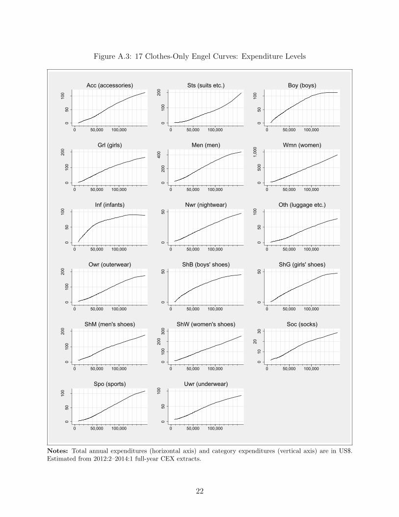
Figure A.3: 17 Clothes-Only Engel Curves: Expenditure Levels50

100

0

0 50,000 100,000

Acc (accessories)

100

200

0

0 50,000 100,000

Sts (suits etc.)

5010

00

0 50,000 100,000

Boy (boys)

100

200

0

0 50,000 100,000

Grl (girls)

200

400

0

0 50,000 100,000

Men (men)

500

1,00

00

0 50,000 100,000

Wmn (women)

5010

00

0 50,000 100,000

Inf (infants)

500

0 50,000 100,000

Nwr (nightwear)

5010

00

0 50,000 100,000

Oth (luggage etc.)

100

200

0

0 50,000 100,000

Owr (outerwear)

500

0 50,000 100,000

ShB (boys' shoes)50

0

0 50,000 100,000

ShG (girls' shoes)

100

200

0

0 50,000 100,000

ShM (men's shoes)

100

200

300

0

0 50,000 100,000

ShW (women's shoes)

1020

300

0 50,000 100,000

Soc (socks)

5010

00

0 50,000 100,000

Spo (sports)

5010

00

0 50,000 100,000

Uwr (underwear)

Notes: Total annual expenditures (horizontal axis) and category expenditures (vertical axis) are in US$.Estimated from 2012:2–2014:1 full-year CEX extracts.

22

Figure A.4: 17 Clothes-Only Engel Curves: Expenditure Shares

.02

.04

.06

.08

00 50,000 100,000

Acc (accessories)

.05

.1

.15

00 50,000 100,000

Sts (suits etc.)

.02

.04

.06

.08.1

00 50,000 100,000

Boy (boys)

.04

.06

.08.1

.12

00 50,000 100,000

Grl (girls)

.2.25

.3

00 50,000 100,000

Men (men)

.3

.4

.5

.6

00 50,000 100,000

Wmn (women)

.05

.1

.15

00 50,000 100,000

Inf (infants)

.024.026.028.03.032

00 50,000 100,000

Nwr (nightwear)

.01

.02

.03

.04

.05

00 50,000 100,000

Oth (luggage etc.)

.08.1

.12

00 50,000 100,000

Owr (outerwear)

.01

.02

.03

.04

00 50,000 100,000

ShB (boys' shoes)

.01

.02

.03

.04

00 50,000 100,000

ShG (girls' shoes)

.11.12.13.14

00 50,000 100,000

ShM (men's shoes)

.12.13.14.15.16

00 50,000 100,000

ShW (women's shoes)

.018.02.022

00 50,000 100,000

Soc (socks)

.03

.04

.05

.06

.07

00 50,000 100,000

Spo (sports)

.05

.06

.07

.08

.09

00 50,000 100,000

Uwr (underwear)

Notes: Total annual expenditures (horizontal axis) are in US$. Category expenditure shares (vertical axis)are in percent of total expenditures. Estimated from 2012:2–2014:1 full-year CEX extracts.

23