expectation propagation of gaussian process classification...
TRANSCRIPT

Expectation Propagation of Gaussian ProcessClassification and Its Application to Gene
Expression Analysis
Mingyue TanDepartment of Computer ScienceUniversity of British Columbia
Abstract
Expectation Propagation (EP) is an approximate Bayesian infer-ence technique which has been applied to Gaussian Process Clas-sification (GPC) [4]. In this paper, we investigate four differentlikelihood functions of GPC, and present EP algorithms for each ofthese four models. We compare the performances of these modelson synthetic data in circular shape. Comparative study is per-formed on EP-GPC with SVM and Laplace-GPC. Experimentalresults show EP-GPC outperforms the other two kernel methodson high dimensional gene expression data. A feature selection tech-nique, Automatic Relevance Determination (ARD), is applied tofind the relevance of genes. Experiments show the effectiveness ofARD for all classification models.
1 Introduction
Classification with kernel machines have recently received much attention from themachine learning community. Some popular kernel classification algorithms includeSupport Vector Machine (SVM) [8], Bayes Point Machine (BPM), and GPC [5].In this paper, we focus on GPC which is a Bayesian kernel classifier derived fromGaussian process priors over functions. Further more, we focus on he binary classi-fication,i.e. discrimination between classes labeled as -1/+1.
GPCs can be represented as graphical models which have random variables forinputs, latent variables for function values, and class labels. Class labels are com-pletely determined by the latent function values. Several noise model can be usedto model the likelihood of class label given the latent value, such as probit function.Automatic Relevance Determination (ARD) parameters can be directly embeddedinto the covariance function, which can be considered a kernel that simplifies theproblem in high dimensional space [5].
Since only class labels are observed, we need to integrate over both hyperparametersand latent values of these functions at the data points. Many approximation tech-niques have been used to approximate the integrals. For example, Williams used a

Figure 1: Graphical model for GPCs with n training data points and one test datapoint. [3]
Laplace approximation to integrate over the latent values and Hybrid Monte Carlo(HMC) to integrate over the hyperparamters [9]. Neal used HMC to integrate overboth latent values and hyperparameters [5]. However, Monte Carlo methods aresometimes expensive to use in practice. A successful approach using ExpectationPropagation (EP) is introduced by Thomas Minka in [4].
The contributions of this paper include: (1)Investigation of four different likelihoodfunctions, namely step function, probit function, probit function with bias, probitfunction with Gaussian noise, for GPC and derive EP update rules for probit func-tion with and without Gaussian noise. (2)Implementation of EP-GPC using probitfunction and probit function with bias. (3)Comparative study on various likelihoodfunctions in the literature of EP for GPC (4) Comparative study of EP with otherapproximate inference techniques, such as Laplace approximation, as applied toGPC.
The rest of the paper is organized as follows. Section 2 introduces Gaussian processclassification. In Section 3, we discuss EP with variational methods for hyperparam-eter inference. Section 4 presents EM-EP algorithm with four likelihood functions.The experimental results on both synthetic data and real gene expression data arereported in Section 5. We conclude in Section 6.
2 Gaussian Process Classifiers
Consider a data set D of data points xi with binary class labels yi ∈ {−1, 1},D = {(xi, yi)|i = 1, 2, ..., n}, X = {xi|i = 1, 2, ...n}, Y = {yi|i = 1, 2, ..., n}. Giventhis training data set, we wish to predict the class label for a new data point x∗ bycomputing the class probability p(y∗|x∗, D).
The main idea of Gaussian process classifier is to assume that the class label yi isobtained by transforming some real valued latent variable f(xi) associated with xi.The graphical model for GPC is shown in Figure 1. This graphical model encodesthe assumption that x and y are independent given f . A bayesian framework isdescribed with more details in the following.
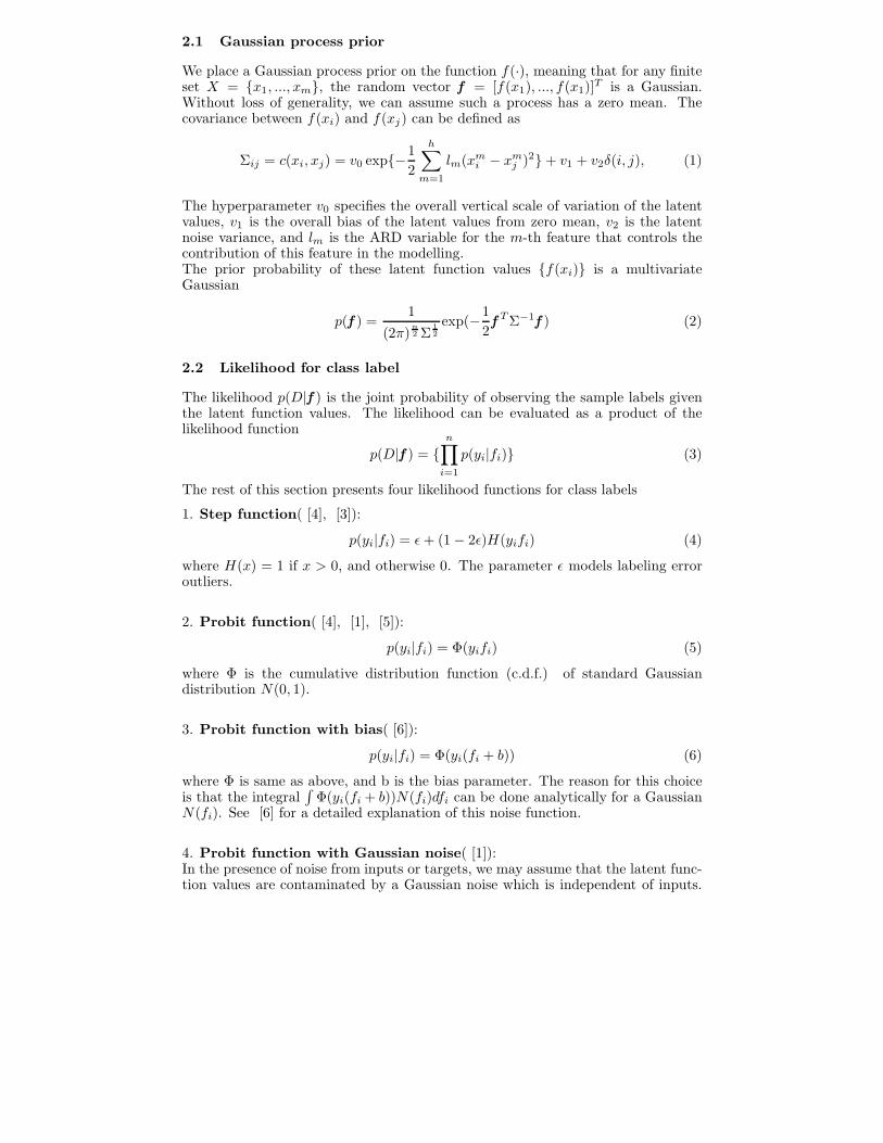
2.1 Gaussian process prior
We place a Gaussian process prior on the function f(·), meaning that for any finiteset X = {x1, ..., xm}, the random vector f = [f(x1), ..., f(x1)]T is a Gaussian.Without loss of generality, we can assume such a process has a zero mean. Thecovariance between f(xi) and f(xj) can be defined as
Σij = c(xi, xj) = v0 exp{−12
h∑m=1
lm(xmi − xm
j )2} + v1 + v2δ(i, j), (1)
The hyperparameter v0 specifies the overall vertical scale of variation of the latentvalues, v1 is the overall bias of the latent values from zero mean, v2 is the latentnoise variance, and lm is the ARD variable for the m-th feature that controls thecontribution of this feature in the modelling.The prior probability of these latent function values {f(xi)} is a multivariateGaussian
p(f ) =1
(2π)n2 Σ
12exp(−1
2f T Σ−1f ) (2)
2.2 Likelihood for class label
The likelihood p(D|f ) is the joint probability of observing the sample labels giventhe latent function values. The likelihood can be evaluated as a product of thelikelihood function
p(D|f ) = {n∏
i=1
p(yi|fi)} (3)
The rest of this section presents four likelihood functions for class labels
1. Step function( [4], [3]):
p(yi|fi) = ε + (1 − 2ε)H(yifi) (4)
where H(x) = 1 if x > 0, and otherwise 0. The parameter ε models labeling erroroutliers.
2. Probit function( [4], [1], [5]):
p(yi|fi) = Φ(yifi) (5)
where Φ is the cumulative distribution function (c.d.f.) of standard Gaussiandistribution N(0, 1).
3. Probit function with bias( [6]):
p(yi|fi) = Φ(yi(fi + b)) (6)
where Φ is same as above, and b is the bias parameter. The reason for this choiceis that the integral
∫Φ(yi(fi + b))N(fi)dfi can be done analytically for a Gaussian
N(fi). See [6] for a detailed explanation of this noise function.
4. Probit function with Gaussian noise( [1]):In the presence of noise from inputs or targets, we may assume that the latent func-tion values are contaminated by a Gaussian noise which is independent of inputs.

If we use δ to denote the noise, then δ has zero mean and an unknown variance σ2,i.e. N(δ; 0, σ2). The likelihood function becomes
p(yi|fi) = Φ(yifi
σ); (7)
2.3 Posterior probability
The posterior probability can be written as
p(f |D) =1
p(D)
n∏i=1
p(yi|fi)p(f ) (8)
where the prior probability p(f ) is defined as in (2), and p(D) =∫
p(D|f )p(f )df
The kernel parameters in the covariance function (1), and labeling error ε in stepfunction, bias term b in probit bias function, or the noise variance σ in probit noisefunction are all collected into θ, which we will call hyperparameters. The normaliza-tion factor p(D) in (8), which should be conditional on the hyperparameters p(D|θ),also known as evidence for θ is a yardstick for model selection. Section (3) discusseshow EP can be used for hyperparameter learning.
2.4 Prediction
Suppose we have found the optimal settings of hyperparameters θ∗, then let ustake a test sample x∗, for which the class label y∗ is unknown. By the definition ofGaussian process, the latent variable f(x∗) and the f = [f(x1), ..., f(xn)]T have ajoint multivariate Gaussian distribution, i.e.
[ff∗
]∼ N
[ (00
),
(Σ k
kT K(x∗, x∗)
) ]
where k = [K(x∗, x1),K(x∗, x2), ...,K(x∗, xn)]T . The conditional distribution off(x∗) given f is also a Gaussian:
p(f∗|f , D, θ∗) ∝ exp
(−1
2(f(x∗) − f T Σ−1k)2
K(x∗, x∗) − kT Σ−1k
)(9)
The predictive distribution of P (f(x∗)|D, θ∗) can be computed as
p(f∗|D, θ∗) =∫
p(f∗|f , D, θ∗)p(f |D, θ∗)df (10)
The second term of the integrand, the posterior distribution p(f |D, θ∗) can beapproximated as a Gaussian by the EP approach discussed in section (3). Thepredictive distribution (10) then can be simplified as a Gaussian N(f(x∗); µx∗ , σx∗
2)with mean µx∗ and variance σx∗
2. In the EP approach, we reach
µx∗ = kT (Σ + Π−1)−1m and σx∗2 = K(x∗, x∗) − kT (Σ + Π−1)−1k (11)
The predictive distribution over the class label y∗ is

p(y∗|x∗, D, θ∗) =∫
p(y∗|f(x∗), θ∗)p(f(x∗)|D, θ∗) df(x∗) (12)
=
⎧⎪⎪⎪⎪⎨⎪⎪⎪⎪⎩
1 − normcdf(0, µx∗ , σx∗) step functionΦ( y∗µx∗√
1+σx∗2) probit function
Φ(y∗(µx∗+b)√1+σx∗2
) probit function with bias
Φ( y∗µx∗√σ2+σx∗2
) probit function with Gaussian noise
(13)
where normcdf(x, µ, σ) is the cumulative density of a normal distribution with meanµ and variance σ from −∞ to x.
The class label yx∗ can be decided as
argmaxi
p(y∗ = i|x∗, D, θ∗)
As for the step function, the class label has a special form of
arg maxi
p(y∗ = i|x∗, D, θ∗) = sgn(n∑
i=1
yi
λi
(1 − 2ε)N(zi; 0, 1)ε + (1 − 2ε)erf(zi)
K(xi, x∗))
where zi and λi for step function are defined in the same way as in [3],
3 EP for Gaussian Process Classifiers
Expectation Propagation (EP) algorithm is an approximation Bayesian inferencetechnique that tries to minimize the KL-divergence between the true posterior andthe approximation [4]. We review EP in its general form before describing itsapplication to GPCs.
The EP algorithm has been applied in GPCs along with variational methods formodel selection ( [6], [3], [1]). In the settings of Gaussian processes, EP at-tempts to approximate p(f |D) as a product distribution in the form of q(f ) =∏n
i=1 ti(f(xi))p(f ) where ti(f(xi)) = siexp(− 12pi(f(xi) − mi)2).
The parameters si, mi, pi in ti are successively optimized by minimizing the follow-ing Kullback-Leibler divergence,
tnewi (f ) = arg min
ti
KL(q(f )toldi
p(yi|f(xi))||q(f )toldi
ti) (14)
Since q is in the exponential family, this minimization is solved by matchingmoments of the approximated distribution. EP iterates over i until convergence.A detailed updating scheme for EP-GPC with probit functions (with and withoutGaussian noise) can be found in Appendix A. The algorithm is not guaranteedto converge although it did in practice. At equilibrium of q(f ), we obtain anapproximate posterior distribution as
p(f |D) ≈ N(f ; (Σ−1 + Π)−1Πm , (Σ−1 + Π)−1) (15)where Π is the diagonal matrix whose ii-th entry is pi and m = [m1, ..., mn]T .
Variational methods can be used to optimize the hyperparameter θ by maximizethe lower bound of the logarithm of the evidence, which has the following form

log p(D|θ) = log∫
p(D|f )p(f )q(f )
q(f )df ≥∫
q(f )logp(D|f )p(f )
q(f )df
=∫
q(f )logp(D|f )df +∫
q(f )logp(f )df −∫
q(f )logq(f )df = F (θ)
(16)
Given the expression of the lower bound F (θ) in terms of q(f ), the gradients ofF (θ) with respect to θ can be derived by neglecting the possible dependency ofq(f ) on F (θ). The detailed formulation can be found in Appendix B.
4 The EM-EP Algorithm
Kim and Ghahramani [3] proposed a conceptually simple EM-like algorithm tolearn the hyperparameters which we refer as EM-EP algorithm. The algorithmworks as follows.
1. E-step EP iterations are performed given the hyperparameters. p(f |D) is ap-proximated as a Gaussian density q(f ) given by Equation (15)See Appendix A for the EP algorithm for the four models
2. M-step Given q(f ) obtained from the E-step, find the hyperparameters whichmaximize the variational lower bound of logp(D|θ).The E-step and the M-step are alternated until convergence. See Appendix Bfor a derivation of the M-step. The gradient update rules with respect to thehyperparameters can be found in Appendix B.
5 Experimental Results
One of the goals of this paper is to compare various likelihood functions of GPCusing EP. We start this section with two simple synthetic datasets in circular shapeto visualize the behavior of these algorithms. Another goal of this paper is tocompare EP with other inference techniques, such as Laplace approximation, forGPC. To do this, we test EP-GPC and Laplace-GPC on gene expression data, andthe performances of these two algorithms are compared with SVM.
5.1 Implementation
Based on Kim’s matlab code of EM-EP algorithm with step likelihood function, weimplemented EM-EP algorithm with two other likelihood functions, namely probitfunction and probit function with bias. Chu [1] publishes his C code of GPC forordinal regression. By some simple algebra, we can see that in the case of binaryclassification, the generalized likelihood function in Chu’s ordinal regression modelbecomes the probit function with Gaussian noise, so we use his code to test thislikelihood function.In the first experiment with two dimensional synthetic datasets, we use Kim’s mat-lab code, our matlab code, and Chu’s C code to test various likelihood functions.Because of the lower speed of matlab implementation, we only use Chu’s C code totest EP for GPC on high dimensional gene expression data.

5.2 Synthetic Data
We use the same data as in [3]. The two-dimensional data set with input features(i.e. dimensions) x1 and x2 are random numbers between -1 and 1. The decisionrule for class -1 and +1 is x2
1 + x22 ≥ 0.5. A total of 1000 data points are generated
with 40 of them as the training set and the remaining 960 samples as the test set.Two such type of datasets are used. The two data sets are same excepted that weadded labeling errors to two randomly selected data points in the training set. Testresults are shown in Figure 2-8.
For the step function, we compare the case where labeling error hyperparameter εis fixed (ε = 0) to the one with adapted labeling error hyperparameter on the twodatasets. For the dataset without outliers, the model with fixed ε achieves the sametest error rate as the one with adapted ε. Classification results are shown in Figure2. However, the model with fixed ε converges faster as shown in Figure 3. Thismakes sense because it takes time for parameters, in this case ε, with improper initialsetting to be adapted. In the presence of outliers, The algorithm with adapted εoutperforms the one with fixed ε, because fixed ε can cause overfitting as shown inFigure 4. The convergence properties of the algorithms are shown in Figure 5.
Three versions of probit functions can not handle the dataset in circular shape well.The algorithm with either version of probit function achieves a test error rate of12% or so. Classification results with one type of probit function is shown in Figure6. The algorithms using probit functions fail if the data contain outliers. As shownin Figure 7, the classificaiton performances of the classifiers with probit functionsare no better than random guess in presence of outliers. This may suggest thatprobit function models a general dependency (with tractable noise) of class labelson latent function values, not extreme case, like outlyingness or mislabelling.
5.3 Gene Expression Data
We applied the algorithm using probit function with Gaussian noise to high-dimensional gene expression dataset: colon cancer.
For the colon dataset, the task is to discriminate tumor from normal tissues. Thedataset has 22 normal and 40 cancer samples with 2000 features per sample. Werandomly split the dataset into 42 training and 20 test samples 10 times and runSVM, EP-GPC, and Laplace-GPC on each partition. Test results of the threealgorithms using linear kernels are presented in Table 1 and Table 2. Note thateven though Laplace approach reaches a smaller variance in the case where all 2000features are used, the test error rates on this dataset are both large. It makes senseto use predictive variance as a criteria to evaluate classification performance only ifthe classification accuracy is reasonably well.
By using some feature selection techniques, such that ARD, we can eliminatedirrelevant features. In this case, we use the dataset containing 373 relevant featuresselected according to optimal ARD parameter values. All of the three algorithmsachieve higher accuracies on this smaller dataset, and the two GPCs outperformSVM. EP-GPC and Laplace-GPC have comparative classification accuracies, butEP-GPC approach is better than Laplace-GPC in the sense that the variance of thepredictive distribution using EP is smaller.

6 Conclusion and Future Work
Based on the work of [4, 6, 1] on noise models, and EM-EP algorithm proposed in[3], we investigate four likelihood functions and derive some special form of updatingrules for EM-EP algorithms in the case of binary classification. Experiments showedstep function with labeling error hyperparameter handles outliers well. GPC withEM-EP showed better performances than both SVM and GPC with Laplace-MAPon gene expression data. By incorporating some Bayesian feature selection tech-niques, such as ARD, we can improve the performance of GPCs on high dimensionaldata.
GPCs have some advantages over other kernel methods because they are fully sta-tistical models. This suggests that we can improve the performance of GPCs frommany different directions. For example, we can incorporate prior information to in-form learning of the hyperparameters. We can improve approximate inference andoptimization techniques to gain in both accuracy and speed. Also, a good follow-upof this project is to build a better likelihood function. Experiments show step func-tion handles outliers well, and we believe probit functions may handle general noisydata better. As future work, we can do experiments to verify our hypothesis. Inreal world, Microarray gene expression data are usually both mislabeled and noisy.A robust likelihood function which captures both properties is desired.
Acknowledgements
Thanks to Dr. Kevin Murphy for directing papers on the topics of EP for GPC.Thanks to H. Kim for providing his matlab code of EMEP for GPC with steplikelihood function. Thanks to W. Chu for providing the C code of GPC for ordinalregression and gene expression data.
Appendix A. Approximate posterior distribution by EP 1
The EP algorithm using step likelihood function and probit function with bias arepresented in [3] and [6] respectively. We skip these algorithms because of thelimited space. The updating scheme of EP algorithm for the other two likelihoodfunctions, namely probit function and probit function with Gaussian noise, arepresented below.
1. Initialization (same for all likelihood functions)
• individual mean mi = 0 ∀i;
• individual inverse variance pi = 0 ∀i;
• individual amplitude si = 1 ∀i
• posterior covariance Ai = (Σ−1 + Π)−1, where Π = diag(p1, p2, ..., pn);
• posterior mean h = AΠm , where m = [m1, m2, ..., mn]T .
2. Looping from i = 1, ..., n until all (mi, pi, si) converge:
(1) Remove ti from the posterior q(f ) to get a leave-one-out posterior distributionq\i(f ) having
1A major portion of the fomulae in this Appendix is based [1]’s work on ordinalregression, and we present the special form for binary classification

- variance of fi: λ\ii = Aii
1−Aii
- mean of fi: h\ii = hi + λiv
−1i (hi − mi)
- others with j = i : λ\ii = Ajj and h
\ij = hj
(2) Compute new posterior approximation by incorporating the message p(yi|fi)into q\i(f):
If Probit Function with Gaussian noise 2 is used, then- Zi =
∫ P(yi|f(xi))N (f(xi); h\ii , λ
\ii )df(xi) = Φ(zi)
where zi = yih\ii√
λ\ii +σ2
αi = ∂ logZi
∂h\ii
= − 1√λ\ii +σ2
(N (zi;0,1)Φ(zi)
)
βi = ∂ logZi
∂λ\ii
= − 1
2(λ\ii +σ2)
(yiziN (zi;0,1)Φ(zi)
)
- vi = α2i − 2βi
- hnewi = h
\ii + λ
\ii αi
- pnewi = vi
1−λ\ii vi
- mnewi = h
\ii + αi
vi
- snewi = Zi
√λ\ii pnew
i + 1exp( α2i
2vi)
(3) If pnewi > 0, update {pi, mi, si}, the posterior mean h and covariance A.
• Anew = A − ρaiaTi where ρ = pnew
i −pi
1+(pnewi −pi)Aii
and ai is the i-th column ofA. (if pnew
i ≈pi, skip this sample and this updating.)
• hnew = h + ηai where η = αi+pi(hi−mi)1−Aiipi
The approximate evidence can be obtained in the same way as for BPMs:P(D | θ) at the EP solution, which can be written as
n∏i=1
sidet
12 (∏−1)
det12 (∑
+∏−1)
exp(B
2)
where B =∑
ij Aij(mipi)(mjpj) −∑
i pim2i
Appendix B. Gradient Formulae for Variational Bound
At the equilibrium of q(f ), the variational bound F can be analytically calculatedas follows:
2If probit function is used for likelihood, simply replace every occurrence of σ2 by 1 inthe expressions of Zi, zi, αi, and βi.

F(θ) =n∑
i=1
∫N(f(xi); hi, Aii) ln(p(yi|f(xi)))df(xi) − 1
2ln |I + ΣΠ|
−12trace((I + ΣΠ)−1) − 1
2mT (Σ + Π−1)−1Σ(Σ + Π−1)−1m +
n
2(17)
Again, we skip the gradient formulae for step function. Refer to [3] if interested.Let κ denote the vector containing the hyperparameters in covariance function, bdenote the bias in the probit function with bias, and θ denote the noise variance inprobit function with Gaussian noise. Then the gradient of F(θ) with respect to thevariables lnκ, ln b, ln σ can be given in the following:
∂F(θ)∂ ln κ
= κ
∫Q(f )
∂ logP(f )∂κ
df
= −κ
2trace(Σ−1 ∂Σ
∂κ) +
κ
2hT Σ−1 ∂Σ
∂κΣ−1h +
κ
2trace(Σ−1 ∂Σ
∂κΣ−1A)
= −κ
2trace((Π−1 + Σ)−1 ∂Σ
∂κ) +
κ
2mT (Π−1 + Σ)−1 ∂Σ
∂κ(Π−1 + Σ)−1m
(18)
∂F(θ)∂ ln σ
= σ
n∑i=1
∫N (f(xi); hi,Aii)
∂ lnP(yi | f(xi))∂σ
df(xi)
=n∑
i=1
yi
∫N (f(xi);
hiσ2
σ2 + Aii,
σ2Aii
σ2 + Aii)
−f(xi)√2π(σ2+Aii)
exp(− (hi)2
2(σ2+Aii))
P(yi | f(xi))df(xi)
(19)
∂F(θ)∂ ln b
=n∑
i=1
∫N (f(xi); hi,Aii)
(fi − hi)Aii
ln Φ(yi(f(xi) + b))df(xi) (20)
The last two integrals can be approximated using Gaussian quadrature.
References
[1] Chu, W. & Z. Ghahramani. Gaussian processes for ordinal regres-sion. Technical report, Gatsby Unit, University College London, 2004.www.gatsby.ucl.ac.uk/ chuwei/paper/gpor.pdf
[2] Qi, Y., T.P.Minka, R.W.Picard, & Z. Ghahramani. Predictive automatic relevancedetermination by expectation propagation. In Proceedings of the Twenty-first Inter-national Conference on Machine Learning, pages 671-678, 2004.
[3] Kim, H. & Z. Ghahramani. The EM-EP algorithm for Gaussian process classification.In Proceedings of the Workshop on Probabilistic Graphical Models for Classification(at ECML), 2003
[4] Minka, T.P. A family of algorithm for approximate Bayesian inference. Ph.D. thesis,Massachusetts Institute of Technology, Janurary 2001.
[5] Neal, R. M. Monte Carlo implementation of Gaussian process models for Bayesianregression and classification. Technical Report No. 9702, Department of Statistics,University of Toronto, 1997.

[6] Seeger, M. Notes on Minka’s expectation propagation for Gaussian process classifica-tion. Technical report, University of Edinburgh, 2002.
[7] Rasmussen, C.R. Gaussian Process in Machine Learning. Advanced Lectures on Ma-chine Learning: ML Summer Schools 2003, Canberra, Australia, February 2 - 14,2003, Tubingen, Germany, August 4 - 16, 2003.
[8] Rasmussen, V. The Nature of Statistical Learning Theory. Springer, New York(1995).
[9] Williams, C.K.I and D. Barber. Bayesian classification with Gaussian processes. IEEETransactions on Pattern Analysis and Machine Intelligence, 20(12):1342-1351, 1998.

Figure 2: Classification Results on Data without Outliers Using Step Function
(a) Training set, (b) Test set, (c) Classification result on training data using the optimal hyperparameter settings trained with the training set, (d) Classification result on test set
(a) fixed ε (ε= 0) (b) adapted ε (ε= 0.01 initially)
Figure 3: Logarithm of Evidence at Each Iteration on Data without outliers using Step Function
The evidence converges faster with fixed labeling error (ε= 0) than the case where ε was adapted.

Figure 4: Classification Results on Data with Outliers Using Step Function
(a) Training set with two outliers, i.e. data points that are mislabeled, which are circled red, (b) Test set, (c) Classification result with fixed labeling error hyperparameter (ε= 0), (d) Classification result with adapted labeling error hyperparameter ε
(a) fixed ε (ε= 0) (b) adapted ε (ε= 0.01 initially)
Figure 5: Logarithm of Evidence at Each Iteration on Data with Outliers using Step Function

Figure 6: Classification Results on Data without outliers Using Probit functions
Figure 7: Classification Results on Data with outliers Using Probit functions

Algorithms Test Error Rate (%) Predictive Variance SVM 0.226 - Laplace-MAP 0.219 3.49 EP 0.19 6.72
Table 1. Test error rates with all 2000 genes
Algorithms Test Error Rate (%) Predictive Variance SVM 0.216 - Laplace-MAP 0.133 3.16 EP 0.133 4.15
Table 2. Test error rates with 373 relevant genes