expdesign.ppt
TRANSCRIPT

8/14/2019 expdesign.ppt
http://slidepdf.com/reader/full/expdesignppt 1/80
Experimental Design and the
Analysis of Variance

8/14/2019 expdesign.ppt
http://slidepdf.com/reader/full/expdesignppt 2/80
Comparing t > 2 Groups - Numeric Responses
• Extension of Methods used to Compare 2 Groups
• Independent Samples and Paired Data Designs
• Normal and non-normal data distributions
Data
Design
Normal Non-
normal
Independent
Samples
(CRD)
F-Test
1-Way
ANOVA
Kruskal-
Wallis Test
Paired Data
(RBD)
F-Test
2-Way
ANOVA
Friedman’s
Test

8/14/2019 expdesign.ppt
http://slidepdf.com/reader/full/expdesignppt 3/80

8/14/2019 expdesign.ppt
http://slidepdf.com/reader/full/expdesignppt 4/80
1-Way ANOVA for Normal Data (CRD)
• For each group obtain the mean, standard deviation, and
sample size:
1
)(2
.
.
i
j
iij
i
i
j
ij
in
y y
sn
y
y
• Obtain the overall mean and sample size
N
y
N
yn yn ynn N
i j ijt t
t
..11
..1
......

8/14/2019 expdesign.ppt
http://slidepdf.com/reader/full/expdesignppt 5/80
Analysis of Variance - Sums of Squares
• Total Variation
1)(1 1
2
..
N df y yTSS Total
k
i
n
j ij
i
• Between Group (Sample) Variation
t
i
n
j
t
i T iii
it df y yn y ySST
1 1 1
2
...
2
...1)()(
• Within Group (Sample) Variation
E T Total
E
t
i ii
t
i
n
j iij
df df df SSE SST TSS
t N df sn y ySSE i
1
2
1 1
2
.)1()(

8/14/2019 expdesign.ppt
http://slidepdf.com/reader/full/expdesignppt 6/80
Analysis of Variance Table and F -TestSource of
Variation Sum of Squares
Degrres of
Freedom Mean Square F
Treatments SST t -1 MST=SST/(t-1) F=MST/MSE
Error SSE N-t MSE=SSE/(N-t)Total TSS N-1
• Assumption: All distributions normal with common variance
• H 0
: No differences among Group Means ( 1
t
=0)
• H A: Group means are not all equal (Not all i are 0)
)(:
)9(:..
:..
,1,
obs
t N t obs
obs
F F P val P
Table F F R R MSE
MST F S T

8/14/2019 expdesign.ppt
http://slidepdf.com/reader/full/expdesignppt 7/80

8/14/2019 expdesign.ppt
http://slidepdf.com/reader/full/expdesignppt 8/80
Expected Mean Squares
• 3 Factors effect magnitude of F -statistic (for fixed t )
– True group effects ( 1,…, t)
– Group sample sizes (n1,…,nt)
– Within group variance (s 2)
• F obs = MST / MSE • When H 0 is true ( 1=…= t=0), E ( MST )/ E ( MSE )=1
• Marginal Effects of each factor (all other factors fixed)
– As spread in ( 1,…, t) E ( MST )/ E ( MSE ) – As (n1,…,nt) E ( MST )/ E ( MSE ) (when H 0 false)
– As s 2 E ( MST )/ E ( MSE ) (when H 0 false)

8/14/2019 expdesign.ppt
http://slidepdf.com/reader/full/expdesignppt 9/80
0
0.01
0.02
0.03
0.04
0.05
0.06
0.07
0.08
0.09
0 20 40 60 80 100 120 140 160 180 200
0
0.01
0.02
0.03
0.04
0.05
0.06
0.07
0.08
0.09
0 20 40 60 80 100 120 140 160 180 200
0
0.01
0.02
0.03
0.04
0.05
0.06
0.07
0.08
0.09
0 20 40 60 80 100 120 140 160 180
0
0.01
0.02
0.03
0.04
0.05
0.06
0.07
0.08
0.09
0 20 40 60 80 100 120 140 160 180 200
A) =100, t1=-20, t2=0, t3=20, s = 20 B) =100, t1=-20, t2=0, t3=20, s = 5
C) =100, t1=-5, t2=0, t3=5, s = 20 D) =100, t1=-5, t2=0, t3=5, s = 5
n A B C D4 9 129 1.5 9
8 17 257 2 17
12 25 385 2.5 25
20 41 641 3.5 41
)(
)(
MSE E
MST E

8/14/2019 expdesign.ppt
http://slidepdf.com/reader/full/expdesignppt 10/80
Example - Seasonal Diet Patterns in Ravens
• “Treatments” - t = 4 seasons of year (3 “replicates” each)
– Winter: November, December, January
– Spring: February, March, April
– Summer: May, June, July
– Fall: August, September, October
• Response (Y ) - Vegetation (percent of total pellet weight)
• Transformation (For approximate normality):
100arcsin' Y Y
Source: K.A. Engel and L.S. Young (1989). “Spatial and Temporal Patterns in the Diet of Common
Ravens in Southwestern Idaho,” The Condor , 91:372-378

8/14/2019 expdesign.ppt
http://slidepdf.com/reader/full/expdesignppt 11/80
Seasonal Diet Patterns in Ravens - Data/Means Y Winter(i=1) Fall(i=2) Summer(i=3) Fall (i=4)
j=1 94.3 80.7 80.5 67.8
j=2 90.3 90.5 74.3 91.8
j=3 83.0 91.8 32.4 89.3
Y' Winter(i=1) Fall(i=2) Summer(i=3) Fall (i=4)
j=1 1.329721 1.115957 1.113428 0.967390
j=2 1.254080 1.257474 1.039152 1.280374
j=3 1.145808 1.280374 0.605545 1.237554
135572.112
237554.1...329721.1
16773.13
237554.1280374.1967390.0
919375.03
605545.0039152.1113428.1
217935.13
280374.1257474.1115957.1
24203.13
145808.1254080.1329721.1
..
.4
.3
.2
.1
y
y
y
y
y

8/14/2019 expdesign.ppt
http://slidepdf.com/reader/full/expdesignppt 12/80
Seasonal Diet Patterns in Ravens - Data/Means
Plot of Transformed Data by Season
0.500000
0.600000
0.700000
0.800000
0.900000
1.000000
1.100000
1.200000
1.300000
1.400000
1.500000
0 1 2 3 4 5
Season
T r a n s f o r m e d % V
e g e t a t i o n

8/14/2019 expdesign.ppt
http://slidepdf.com/reader/full/expdesignppt 13/80

8/14/2019 expdesign.ppt
http://slidepdf.com/reader/full/expdesignppt 14/80
Seasonal Diet Patterns in Ravens - Spreadsheet
Month Season Y' Season Mean verall Mean TSS SST SSE
NOV 1 1.329721 1.243203 1.135572 0.037694 0.011584 0.007485DEC 1 1.254080 1.243203 1.135572 0.014044 0.011584 0.000118
JAN 1 1.145808 1.243203 1.135572 0.000105 0.011584 0.009486
FEB 2 1.115957 1.217935 1.135572 0.000385 0.006784 0.010400
MAR 2 1.257474 1.217935 1.135572 0.014860 0.006784 0.001563
APR 2 1.280374 1.217935 1.135572 0.020968 0.006784 0.003899
MAY 3 1.113428 0.919375 1.135572 0.000490 0.046741 0.037657
JUN 3 1.039152 0.919375 1.135572 0.009297 0.046741 0.014346JUL 3 0.605545 0.919375 1.135572 0.280928 0.046741 0.098489
AUG 4 0.967390 1.161773 1.135572 0.028285 0.000687 0.037785
SEP 4 1.280374 1.161773 1.135572 0.020968 0.000687 0.014066
OCT 4 1.237554 1.161773 1.135572 0.010400 0.000687 0.005743
Sum 0.438425 0.197387 0.241038
Total SS Between Season SS Within Season SS
(Y’-Overall Mean)
2
(Group Mean-Overall Mean)
2
(Y’-Group Mean)
2

8/14/2019 expdesign.ppt
http://slidepdf.com/reader/full/expdesignppt 15/80
CRD with Non-Normal Data
Kruskal-Wallis Test
• Extension of Wilcoxon Rank-Sum Test to k > 2 Groups
• Procedure:
– Rank the observations across groups from smallest (1) to largest( N = n1+...+nk ), adjusting for ties
– Compute the rank sums for each group: T 1,...,T k . Note that
T 1+...+T k = N ( N +1)/2

8/14/2019 expdesign.ppt
http://slidepdf.com/reader/full/expdesignppt 16/80
Kruskal-Wallis Test
• H 0: The k population distributions are identical ( 1=...= k )
• H A: Not all k distributions are identical (Not all i are equal)
)(:
:..
)1(3)1(
12
:..
2
2
1,
1
2
H P val P
H R R
N n
T
N N H S T
k
k
ii
i
An adjustment to H is suggested when there are many ties in the
data. Formula is given on page 344 of O&L.

8/14/2019 expdesign.ppt
http://slidepdf.com/reader/full/expdesignppt 17/80
Example - Seasonal Diet Patterns in Ravens
Month Season Y' Rank
NOV 1 1.329721 12
DEC 1 1.254080 8
JAN 1 1.145808 6
FEB 2 1.115957 5
MAR 2 1.257474 9
APR 2 1.280374 10.5
MAY 3 1.113428 4
JUN 3 1.039152 3JUL 3 0.605545 1
AUG 4 0.967390 2
SEP 4 1.280374 10.5
OCT 4 1.237554 7
• T 1 = 12+8+6 = 26
• T 2 = 5+9+10.5 = 24.5
• T 3 = 4+3+1 = 8
• T 4 = 2+10.5+7 = 19.5
1632.)12.5(:value
815.7:)05.0.(.
12.53912.44)112(33
)5.19(
3
)8(
3
)5.24(
3
)26(
)112(12
12:..
sDifferenceSeasonal: differenceseasonal No:
2
2
14,05.
2222
0
H P P
H R R
H S T
H H a

8/14/2019 expdesign.ppt
http://slidepdf.com/reader/full/expdesignppt 18/80
Post-hoc Comparisons of Treatments
• If differences in group means are determined from the F -
test, researchers want to compare pairs of groups. Three
popular methods include:
– Fisher’s LSD - Upon rejecting the null hypothesis of no
differences in group means, LSD method is equivalent to doing pairwise comparisons among all pairs of groups as in Chapter 6.
– Tukey’s Method - Specifically compares all t (t -1)/2 pairs of
groups. Utilizes a special table (Table 11, p. 701).
– Bonferroni’s Method - Adjusts individual comparison error ratesso that all conclusions will be correct at desired
confidence/significance level. Any number of comparisons can be
made. Very general approach can be applied to any inferential
problem

8/14/2019 expdesign.ppt
http://slidepdf.com/reader/full/expdesignppt 19/80
Fisher’s Least Significant Difference Procedure
• Protected Version is to only apply method aftersignificant result in overall F -test
• For each pair of groups, compute the least significant
difference (LSD) that the sample means need to differ
by to conclude the population means are not equal
ij ji
ij ji ji
ji
ij
LSD y y
LSD y y
t N nn
MSE t LSD
..
..
2/
:IntervalConfidencesFisher'
if Conclude
df with11

8/14/2019 expdesign.ppt
http://slidepdf.com/reader/full/expdesignppt 20/80
Tukey’s W Procedure
• More conservative than Fisher’s LSD (minimum
significant difference and confidence interval width arehigher).
• Derived so that the probability that at least one false
difference is detected is (experimentwise error rate)
t
ij ji
ij ji ji
ij
nn
t n
W y y
W y y
N-t qn
MSE t qW
11 useunequal,aresizessampleWhen the
:IntervalConfidencesTukey'
if Conclude
with701 p.11,Tableingiven),(
1
..
..

8/14/2019 expdesign.ppt
http://slidepdf.com/reader/full/expdesignppt 21/80
Bonferroni’s Method (Most General)
• Wish to make C comparisons of pairs of groups with simultaneous
confidence intervals or 2-sided tests
•When all pair of treatments are to be compared, C = t (t -1)/2
• Want the overall confidence level for all intervals to be “correct” to
be 95% or the overall type I error rate for all tests to be 0.05• For confidence intervals, construct (1-(0.05/C))100% CIs for the
difference in each pair of group means (wider than 95% CIs)
• Conduct each test at =0.05/C significance level (rejection region
cut-offs more extreme than when =0.05)
• Critical t -values are given in table on class website, we will use
notation: t /2,C , where C =#Comparisons, = df

8/14/2019 expdesign.ppt
http://slidepdf.com/reader/full/expdesignppt 22/80
Bonferroni’s Method (Most General)
ij ji
ij ji ji
ji
vC ij
B y y
B y y
N-t vt
nn MSE t B
..
..
,,2/
:IntervalConfidences'Bonferroni
if Conclude
)withwebsiteclassongiven(
11

8/14/2019 expdesign.ppt
http://slidepdf.com/reader/full/expdesignppt 23/80
Example - Seasonal Diet Patterns in Ravens
Note: No differences were found, these calculations are onlyfor demonstration purposes
4930.0
3
1
3
1)03013.0(479.3
4540.03
1)03013.0(53.4
3268.0
3
1
3
1)03013.0(306.2
479.353.4306.2303013.0 8,6,025.8,4,05.8,025.
ij
ij
ij
df C df t i
B
W
LSD
t qt n MSE E E
Comparison(i vs j) Group i Mean Group j Mean ifference
1 vs 2 1.243203 1.217935 0.025267
1 vs 3 1.243203 0.919375 0.323828
1 vs 4 1.243203 1.161773 0.081430
2 vs 3 1.217935 0.919375 0.298560
2 vs 4 1.217935 1.161773 0.056162
3 vs 4 0.919375 1.161773 -0.242398

8/14/2019 expdesign.ppt
http://slidepdf.com/reader/full/expdesignppt 24/80
Randomized Block Design (RBD)
• t > 2 Treatments (groups) to be compared
• b Blocks of homogeneous units are sampled. Blocks can be individual subjects. Blocks are made up of t subunits
• Subunits within a block receive one treatment. When
subjects are blocks, receive treatments in random order.
• Outcome when Treatment i is assigned to Block j is
labeled Y ij
• Effect of Trt i is labeled i
• Effect of Block j is labeled b j
• Random error term is labeled ij
• Efficiency gain from removing block-to-block
variability from experimental error

8/14/2019 expdesign.ppt
http://slidepdf.com/reader/full/expdesignppt 25/80
Randomized Complete Block Designs
• Model:
2
1
)(0)(0 s
b b
ijij
t
i
i
ij jiij jiij
V E
Y
• Test for differences among treatment effects:
• H 0: 1 ... t 0 ( 1 ... t )
• H A: Not all i = 0 (Not all i are equal)
Typically not interested in measuring block effects (although
sometimes wish to estimate their variance in the population of
blocks). Using Block designs increases efficiency in making
inferences on treatment effects

8/14/2019 expdesign.ppt
http://slidepdf.com/reader/full/expdesignppt 26/80
RBD - ANOVA F -Test (Normal Data)• Data Structure: (t Treatments, b Subjects)
• Mean for Treatment i:
• Mean for Subject (Block) j:
• Overall Mean:
• Overall sample size: N = bt
• ANOVA:Treatment, Block, and Error Sums of Squares
.i y
j y.
.. y
)1)(1(
1
1
1
2
....
1
2
...
1
2
...
1 1
2
..
t bdf SSBSST TSS y y y ySSE
bdf y yt SSB
t df y ybSST
bt df y yTSS
E jiij
B
b
j j
T
t
i i
t
i
b
j
Total ij

8/14/2019 expdesign.ppt
http://slidepdf.com/reader/full/expdesignppt 27/80
RBD - ANOVA F -Test (Normal Data)
• ANOVA Table: Source SS df MS F
Treatments SST t -1 MST = SST /(t -1) F = MST / MSE
Blocks SSB b-1 MSB = SSB/(b-1)
Error SSE (b-1)(t -1) MSE = SSE /[(b-1)(t -1)]
Total TSS bt -1
• H 0: 1 ... t 0 ( 1 ... t )
• H A: Not all i = 0 (Not all i are equal)
)(:
:..
:..
)1)(1(,1,
obs
t bt obs
obs
F F P val P
F F R R
MSE MST F S T

8/14/2019 expdesign.ppt
http://slidepdf.com/reader/full/expdesignppt 28/80
Pairwise Comparison of Treatment Means
• Tukey’s Method- q in Studentized Range Table with = (b-1)(t -1)
ij ji
ij ji ji
ij
W y y
W y y
b
MSE vt qW
..
..
:IntervalConfidencesTukey'
if Conclude
),(
• Bonferroni’s Method - t -values from table on class
website with = (b-1)(t -1) and C =t (t -1)/2
ij ji
ij ji ji
vC ij
B y y
B y y
b
MSE t B
..
..
,,2/
:IntervalConfidences'Bonferroni
if Conclude
2

8/14/2019 expdesign.ppt
http://slidepdf.com/reader/full/expdesignppt 29/80
Expected Mean Squares / Relative Efficiency • Expected Mean Squares: As with CRD, the Expected Mean
Squares for Treatment and Error are functions of the samplesizes (b, the number of blocks), the true treatment effects
( 1,…, t) and the variance of the random error terms (s 2)
• By assigning all treatments to units within blocks, error
variance is (much) smaller for RBD than CRD (whichcombines block variation&random error into error term)
• Relative Efficiency of RBD to CRD (how many times as
many replicates would be needed for CRD to have as precise of estimates of treatment means as RBD does):
MSE bt
MSE t b MSBb
MSE
MSE CR RCB RE
RCB
CR
)1(
)1()1(),(

8/14/2019 expdesign.ppt
http://slidepdf.com/reader/full/expdesignppt 30/80
Example - Caffeine and Endurance
• Treatments: t =4 Doses of Caffeine: 0, 5, 9, 13 mg
• Blocks: b=9 Well-conditioned cyclists
• Response: yij=Minutes to exhaustion for cyclist j @ dose i
• Data:
Dose \ Subject 1 2 3 4 5 6 7 8 9
0 36.05 52.47 56.55 45.20 35.25 66.38 40.57 57.15 28.34
5 42.47 85.15 63.20 52.10 66.20 73.25 44.50 57.17 35.05
9 51.50 65.00 73.10 64.40 57.45 76.49 40.55 66.47 33.17
13 37.55 59.30 79.12 58.33 70.54 69.47 46.48 66.35 36.20

8/14/2019 expdesign.ppt
http://slidepdf.com/reader/full/expdesignppt 31/80
Plot of Y versus Subject by Dose
0.00
10.00
20.00
30.00
40.00
50.00
60.00
70.00
80.00
90.00
0 1 2 3 4 5 6 7 8 9 10
Cyclist
T i m e t o E x h a u s t i o n
0 mg
5 mg
9mg
13 mg
E l C ff i d E d

8/14/2019 expdesign.ppt
http://slidepdf.com/reader/full/expdesignppt 32/80
Example - Caffeine and EnduranceSubject\Dose 0mg 5mg 9mg 13mg Subj Mea Subj Dev Sqr Dev
1 36.05 42.47 51.50 37.55 41.89 -13.34 178.07
2 52.47 85.15 65.00 59.30 65.48 10.24 104.93
3 56.55 63.20 73.10 79.12 67.99 12.76 162.714 45.20 52.10 64.40 58.33 55.01 -0.23 0.05
5 35.25 66.20 57.45 70.54 57.36 2.12 4.51
6 66.38 73.25 76.49 69.47 71.40 16.16 261.17
7 40.57 44.50 40.55 46.48 43.03 -12.21 149.12
8 57.15 57.17 66.47 66.35 61.79 6.55 42.88
9 28.34 35.05 33.17 36.20 33.19 -22.05 486.06Dose Mean 46.44 57.68 58.68 58.15 55.24 1389.50
Dose Dev -8.80 2.44 3.44 2.91
Squared Dev 77.38 5.95 11.86 8.48 103.68
TSS 7752.773
24)19)(14(653.1261555812.933773.7752
)24.5515.5819.3320.36()24.5544.4689.4105.36(
81900.5558)50.1389(4)24.5519.33()24.5589.41(4
31412.933)68.103(9)24.5515.58()24.5544.46(9
351)9(4773.7752)24.5520.36()24.5505.36(
22
22
22
22
E
B
T
Total
df SSBSST TSS
SSE
df SSB
df SST
df TSS

8/14/2019 expdesign.ppt
http://slidepdf.com/reader/full/expdesignppt 33/80
Example - Caffeine and Endurance
Source df SS MS F
Dose 3 933.12 311.04 5.92Cyclist 8 5558.00 694.75
Error 24 1261.65 52.57
Total 35 7752.77
equalallnotaremeansthat trueConclude
EXCEL)(From 0036.)92.5(:value
01.3:0.05).(.
92.557.52
04.311:..
DosesAmongExistsDifference:
)0(EffectDoseCaffeine No:
24,3,05.
410
F P P
F F R R MSE
MST F S T
H
H
obs
obs
A

8/14/2019 expdesign.ppt
http://slidepdf.com/reader/full/expdesignppt 34/80
Example - Caffeine and Endurance
83.9
9
257.52875.2875.2:Bs'Bonferroni
43.99
157.5290.390.3:sTukey'
24,6,2/05.
24,4,05.
Bt
W qW
Doses High Mean Low Mean Difference Conclude
5mg vs 0mg 57.6767 46.4400 11.2367 5
9mg vs 0mg 58.6811 46.4400 12.2411 9
13mg vs 0mg 58.1489 46.4400 11.7089 39mg vs 5mg 58.6811 57.6767 1.0044 NSD
13mg vs 5mg 58.1489 57.6767 0.4722 NSD
13mg vs 9mg 58.1489 58.6811 -0.5322 NSD

8/14/2019 expdesign.ppt
http://slidepdf.com/reader/full/expdesignppt 35/80
Example - Caffeine and Endurance
79.395.1839
39.6977
)57.52)(1)4(9(
)57.52)(3(9)75.694(8
)1(
)1()1(),(
57.5275.69494:DesignRandomizedCompletelyBlock toRandomizedof EfficiencyRelative
MSE bt
MSE t b MSBbCR RCB RE
MSE MSBbt
Would have needed 3.79 times as many cyclists per dose to have the
same precision on the estimates of mean endurance time.
• 9(3.79) 35 cyclists per dose
• 4(35) = 140 total cyclists

8/14/2019 expdesign.ppt
http://slidepdf.com/reader/full/expdesignppt 36/80
RBD -- Non-Normal Data
Friedman’s Test
• When data are non-normal, test is based on ranks
• Procedure to obtain test statistic:
– Rank the k treatments within each block (1=smallest,
k =largest) adjusting for ties
– Compute rank sums for treatments (T i) across blocks
– H 0: The k populations are identical ( 1=...= k )
– H A: Differences exist among the k group means
)(:
:..
)1(3)1(
12:..
2
2
1,
1
2
r
k r
k
i ir
F P val P
F R R
k bT k bk
F S T

8/14/2019 expdesign.ppt
http://slidepdf.com/reader/full/expdesignppt 37/80
Example - Caffeine and Endurance
Subject\Dose 0mg 5mg 9mg 13mg Ranks 0mg 5mg 9mg 13mg
1 36.05 42.47 51.5 37.55 1 3 4 22 52.47 85.15 65 59.3 1 4 3 2
3 56.55 63.2 73.1 79.12 1 2 3 4
4 45.2 52.1 64.4 58.33 1 2 4 3
5 35.25 66.2 57.45 70.54 1 3 2 4
6 66.38 73.25 76.49 69.47 1 3 4 2
7 40.57 44.5 40.55 46.48 2 3 1 4
8 57.15 57.17 66.47 66.35 1 2 4 3
9 28.34 35.05 33.17 36.2 1 3 2 4Total 10 25 27 28
equalallnotare(Medians)MeansConclude
EXCEL)(From 0026.)2.14(:value-
815.7:)05.0.(.
2.14135180
26856)14)(9(3)28()10()14)(4(9
12:..
ExistsDifferenceDose:
sDifferenceDose No:
2
2
14,05.
22
0
P P
F R R
F S T
H
H
r
r
a

8/14/2019 expdesign.ppt
http://slidepdf.com/reader/full/expdesignppt 38/80
Latin Square Design
• Design used to compare t treatments when there are
two sources of extraneous variation (types of blocks),each observed at t levels
• Best suited for analyses when t 10
• Classic Example: Car Tire Comparison – Treatments: 4 Brands of tires (A,B,C,D)
– Extraneous Source 1: Car (1,2,3,4)
– Extraneous Source 2: Position (Driver Front, Passenger
Front, Driver Rear, Passenger Rear)Car\Position DF PF DR PR
1 A B C D
2 B C D A
3 C D A B
4 D A B C

8/14/2019 expdesign.ppt
http://slidepdf.com/reader/full/expdesignppt 39/80
Latin Square Design - Model
• Model (t treatments, rows, columns, N =t 2) :
TermErrorRandom
ColumntodueEffect
rowtodueEffect
Treatmentof Effect
MeanOverall
.....
^.....
^
.....
^
k
...
^
ijk
j j j
iii
k k
ijk k ik ijk
y y j
y yi
y yk
y
y
b b
b

8/14/2019 expdesign.ppt
http://slidepdf.com/reader/full/expdesignppt 40/80
Latin Square Design - ANOVA & F -Test
)2)(1()1(3)1( Squaresof SumError
1 Squaresof SumColumn
1 Squaresof SumRow
1 Squaresof SumTreatment
1:Squaresof SumTotal
2
2
1
.....
2
1
.....
2
1
.....
2
2
1 1...
t t t t df SSC SSRSST TSS SSE
t df y yt SSC
t df y yt SSR
t df y yt SST
t df y yTSS
E
C
t
j
j
R
t
i
i
T
t
k
k
t
i
t
jijk
• H 0: 1 = … = t = 0 H a: Not all k = 0
• TS: F obs = MST / MSE = (SST/ (t -1))/(SSE /((t -1)(t -2)))
• RR: F obs
F , t -1 , (t -1)(t -2)

8/14/2019 expdesign.ppt
http://slidepdf.com/reader/full/expdesignppt 41/80
Pairwise Comparison of Treatment Means
• Tukey’s Method- q in Studentized Range Table with = (t -1)(t -2)
ij ji
ij ji ji
ij
W y y
W y y
t
MSE vt qW
..
..
:IntervalConfidencesTukey'
if Conclude
),(
• Bonferroni’s Method - t -values from table on class
website with = (t -1)(t -2) and C =t (t -1)/2
ij ji
ij ji ji
vC ij
B y y
B y y
t
MSE t B
..
..
,,2/
:IntervalConfidences'Bonferroni
if Conclude
2

8/14/2019 expdesign.ppt
http://slidepdf.com/reader/full/expdesignppt 42/80
Expected Mean Squares / Relative Efficiency • Expected Mean Squares: As with CRD, the Expected Mean
Squares for Treatment and Error are functions of the samplesizes (t , the number of blocks), the true treatment effects
( 1,…, t) and the variance of the random error terms (s 2)
• By assigning all treatments to units within blocks, error
variance is (much) smaller for LS than CRD (whichcombines block variation&random error into error term)
• Relative Efficiency of LS to CRD (how many times as
many replicates would be needed for CRD to have as
precise of estimates of treatment means as LS does):
MSE t
MSE t MSC MSR
MSE
MSE CR LS RE
LS
CR
)1(
)1(),(

8/14/2019 expdesign.ppt
http://slidepdf.com/reader/full/expdesignppt 43/80
2-Way ANOVA
• 2 nominal or ordinal factors are believed to
be related to a quantitative response
• Additive Effects: The effects of the levels of
each factor do not depend on the levels of
the other factor.
• Interaction: The effects of levels of each
factor depend on the levels of the other
factor
• Notation: ij is the mean response when
factor A is at level i and Factor B at j
2 W ANOVA M d l

8/14/2019 expdesign.ppt
http://slidepdf.com/reader/full/expdesignppt 44/80
2-Way ANOVA - Model
TermsErrorRandom
combinedareBof levelandAof levelneffect whenInteractio
Bfactorof levelof Effect
Afactorof levelof Effect
MeanOverall levelatB,levelatAFactorsreceivingunitontMeasuremen
,...,1,...,1,...,1
ijk
ij
j
i
b
b
b b
thth
th
th
th
ijk
ijk ij jiijk
ji
j
i
jik y
r k b jai y
•Model depends on whether all levels of interest for a factor are
included in experiment:
• Fixed Effects: All levels of factors A and B included
• Random Effects: Subset of levels included for factors A and B
• Mixed Effects: One factor has all levels, other factor a subset

8/14/2019 expdesign.ppt
http://slidepdf.com/reader/full/expdesignppt 45/80
Fixed Effects Model
• Factor A: Effects are fixed constants and sum to 0
• Factor B: Effects are fixed constants and sum to 0
• Interaction: Effects are fixed constants and sum to 0
over all levels of factor B, for each level of factor A,
and vice versa
• Error Terms: Random Variables that are assumed to be
independent and normally distributed with mean 0,
variance s 2
2
1111
,0~000,0 s b b b N i j ijk
b
j
ij
a
i
ij
b
j
j
a
i
i
E l Th lid id f AIDS

8/14/2019 expdesign.ppt
http://slidepdf.com/reader/full/expdesignppt 46/80
Example - Thalidomide for AIDS
• Response: 28-day weight gain in AIDS patients
• Factor A: Drug: Thalidomide/Placebo
• Factor B: TB Status of Patient: TB+/TB-
• Subjects: 32 patients (16 TB+
and 16 TB-
).Random assignment of 8 from each group to
each drug). Data:
– Thalidomide/TB+: 9,6,4.5,2,2.5,3,1,1.5
– Thalidomide/TB-: 2.5,3.5,4,1,0.5,4,1.5,2
– Placebo/TB+: 0,1,-1,-2,-3,-3,0.5,-2.5
– Placebo/TB-: -0.5,0,2.5,0.5,-1.5,0,1,3.5

8/14/2019 expdesign.ppt
http://slidepdf.com/reader/full/expdesignppt 47/80
ANOVA Approach
• Total Variation (TSS ) is partitioned into 4components:
– Factor A: Variation in means among levels of A
– Factor B: Variation in means among levels of B – Interaction: Variation in means among
combinations of levels of A and B that are not due
to A or B alone
– Error: Variation among subjects within the same
combinations of levels of A and B (Within SS)
A l i f i

8/14/2019 expdesign.ppt
http://slidepdf.com/reader/full/expdesignppt 48/80
Analysis of Variance
)1( :Squaresof SumError
)1)(1( :Squaresof SumnInteractio
1 :Squaresof SumBFactor
1 :Squaresof SumAFactor
1 :VariationTotal
1 1 1
2
.
1 1
2
........
1
2
.....
1
2
.....
1 1 1
2
...
r abdf y ySSE
badf y y y yr SSAB
bdf y yar SSB
adf y ybr SSA
abr df y yTSS
E
a
i
b
j
r
k
ijijk
AB
a
i
b
j
jiij
B
b
j
j
A
a
i
i
Total
a
i
b
j
r
k ijk
• TSS = SSA + SSB + SSAB + SSE
• df Total = df A + df B + df AB + df E
ANOVA A h Fi d Eff t

8/14/2019 expdesign.ppt
http://slidepdf.com/reader/full/expdesignppt 49/80
ANOVA Approach - Fixed EffectsSource df SS MS F
Factor A a-1 SSA MSA=SSA/(a-1) FA=MSA/MSEFactor B b-1 SSB MSB=SSB/(b-1) FB=MSB/MSE
Interaction (a-1)(b-1) SSAB MSAB=SSAB/[(a-1)(b-1)] FAB=MSAB/MSEError ab(r-1) SSE MSE=SSE/[ab(r-1)]
Total abr-1 TSS
• Procedure:
• First test for interaction effects
• If interaction test not significant, test for Factor A and B effects
)1(),1()1(),1(,)1(),1)(1(,
1010110
: : :
: : :
0all Not: 0all Not: 0all Not:0...:0...:0...:
BFactorforTestAFactorforTest:nInteractioforTest
r abb Br aba Ar abba AB
B A AB
jaiaija
baab
F F RR F F RR F F RR
MSE
MSB F TS
MSE
MSA F TS
MSE
MSAB F TS
H H H H H H
b b b b b b

8/14/2019 expdesign.ppt
http://slidepdf.com/reader/full/expdesignppt 50/80
Example - Thalidomide for AIDS
Negative
Positive
tb
Placebo Thal idomide
drug
-2.5
0.0
2.5
5.0
7.5
w t g a i n
Report
WTGAIN
3.688 8 2.6984
2.375 8 1.3562
-1.250 8 1.6036
.688 8 1.6243
1.375 32 2.6027
GROUP
TB+/Thalidomide
TB-/Thalidomide
TB+/Placebo
TB-/Placebo
Total
Mean N Std. Deviation
Individual Patients Group Means
Placebo Thal idomide
drug
-1.000
0.000
1.000
2.000
3.000
m e a n w g

8/14/2019 expdesign.ppt
http://slidepdf.com/reader/full/expdesignppt 51/80
Example - Thalidomide for AIDS
Tests of Between-Subjects Effects
Dependent Variable: WTGAIN
109.688a 3 36.563 10.206 .000
60.500 1 60.500 16.887 .000
87.781 1 87.781 24.502 .000.781 1 .781 .218 .644
21.125 1 21.125 5.897 .022
100.313 28 3.583
270.500 32
210.000 31
Source
Corrected Model
Intercept
DRUG
TB
DRUG * TB
Error
Total
Corrected Total
Type III Sum
of Squares df Mean Square F Sig.
R Squared = .522 (Adjusted R Squared = .471)a.
• There is a significant Drug*TB interaction (FDT=5.897, P=.022)
• The Drug effect depends on TB status (and vice versa)
C i M i Eff (N I i )

8/14/2019 expdesign.ppt
http://slidepdf.com/reader/full/expdesignppt 52/80
Comparing Main Effects (No Interaction)
• Tukey’s Method- q in Studentized Range Table with = ab(r -1)
B ji ji
A ji ji
B
ji ji
A
ji ji
B A
ijij
ijij
ijij
W y yW y y
W y yW y y
ar
MSE vbqW
br
MSE vaqW
........
........
:)(:)(:CIsTukey'
if if :Conclude
),(),(
b b
b b
• Bonferroni’s Method - t -values in Bonferroni table with =ab (r -1)
B
ji ji
A
ji ji
B
ji ji
A
ji ji
vbb
B
vaa
A
ijij
ijij
ijij
B y y- B y y-αα
B y y B y y
ar
MSE t Bbr
MSE t B
........
........
,2/)1(,2/,2/)1(,2/
:)(:)(:CIs'Bonferroni
if if :Conclude
22
b b
b b
C i M i Eff t (I t ti )

8/14/2019 expdesign.ppt
http://slidepdf.com/reader/full/expdesignppt 53/80
Comparing Main Effects (Interaction)
• Tukey’s Method- q in Studentized Range Table with = ab(r -1)
AinBFactorforSimilar:)(:CIsTukey'
if :ConcludeB,Factorof levelk Within
),(
..
..
A jk ik ji
A
jk ik ji
th
A
ij
ij
ij
W y y
W y y
r
MSE vaqW
• Bonferroni’s Method - t -values in Bonferroni table with =ab (r -1)
A
jk ik ji
A
jk ik ji
vaa
A
ij
ij
ij
B y y-αα
B y y
r
MSE t B
..
..
th
,2/)1(,2/
:)(:CIs'Bonferroni
if :ConcludeB,of levelk Within
2

8/14/2019 expdesign.ppt
http://slidepdf.com/reader/full/expdesignppt 54/80
Miscellaneous Topics
• 2-Factor ANOVA can be conducted in a Randomized
Block Design, where each block is made up of ab
experimental units. Analysis is direct extension of
RBD with 1-factor ANOVA
• Factorial Experiments can be conducted with anynumber of factors. Higher order interactions can be
formed (for instance, the AB interaction effects may
differ for various levels of factor C ).
• When experiments are not balanced, calculations are
immensely messier and you must use statistical
software packages for calculations
i d ff d l

8/14/2019 expdesign.ppt
http://slidepdf.com/reader/full/expdesignppt 55/80
Mixed Effects Models
• Assume:
– Factor A Fixed (All levels of interest in study)
1 2 … 0
– Factor B Random (Sample of levels used in study)
b j ~ N(0,s b2) (Independent)
• AB Interaction terms Random
b)ij ~ N(0,sab2 (Independent)
• Analysis of Variance is computed exactly as inFixed Effects case (Sums of Squares, df’s, MS’s)
• Error terms for tests change (See next slide).
ANOVA Approach Mixed Effects

8/14/2019 expdesign.ppt
http://slidepdf.com/reader/full/expdesignppt 56/80
ANOVA Approach – Mixed EffectsSource df SS MS F
Factor A a-1 SSA MSA=SSA/(a-1) FA=MSA/MSABFactor B b-1 SSB MSB=SSB/(b-1) FB=MSB/MSAB
Interaction (a-1)(b-1) SSAB MSAB=SSAB/[(a-1)(b-1)] FAB=MSAB/MSEError ab(r-1) SSE MSE=SSE/[ab(n-1)]
Total abr-1 TSS
• Procedure:
• First test for interaction effects
• If interaction test not significant, test for Factor A and B effects
)1)(1(),1(,)1)(1(),1(,)1(),1)(1(,
22
2
010
2
0
: : :
: : :
0: 0all Not: 0 :0: 0...: 0:
BFactorforTestAFactorforTest:nInteractioforTest
bab Bbaa Ar abba AB
B A AB
baiaaba
baab
F F RR F F RR F F RR
MSAB
MSB F TS
MSAB
MSA F TS
MSE
MSAB F TS
H H H H H H
s s s s
C i M i Eff t f A (N I t ti )

8/14/2019 expdesign.ppt
http://slidepdf.com/reader/full/expdesignppt 57/80
Comparing Main Effects for A (No Interaction)
• Tukey’s Method- q in Studentized Range Table with = (a-1)(b-1)
A
ji ji
A
ji ji
A
ij
ij
ij
W y y
W y y
br
MSABvaqW
....
....
:)(:CIsTukey'
if :Conclude
),(
• Bonferroni’s Method - t -values in Bonferroni table with = (a-1)(b-1)
A
ji ji
A
ji ji
vaa
A
ij
ij
ij
B y y-αα
B y y
br
MSAB
t B
....
....
,2/)1(,2/
:)(:CIs'Bonferroni
if :Conclude
2
R d Eff M d l

8/14/2019 expdesign.ppt
http://slidepdf.com/reader/full/expdesignppt 58/80
Random Effects Models
• Assume:
– Factor A Random (Sample of levels used in study)
i ~ N(0,sa2) (Independent)
– Factor B Random (Sample of levels used in study)
b j ~ N(0,s b2) (Independent)
• AB Interaction terms Random
b)ij ~ N(0,sab2 (Independent)
• Analysis of Variance is computed exactly as inFixed Effects case (Sums of Squares, df’s, MS’s)
• Error terms for tests change (See next slide).
ANOVA Approach Mixed Effects

8/14/2019 expdesign.ppt
http://slidepdf.com/reader/full/expdesignppt 59/80
ANOVA Approach – Mixed EffectsSource df SS MS F
Factor A a-1 SSA MSA=SSA/(a-1) FA=MSA/MSABFactor B b-1 SSB MSB=SSB/(b-1) FB=MSB/MSAB
Interaction (a-1)(b-1) SSAB MSAB=SSAB/[(a-1)(b-1)] FAB=MSAB/MSEError ab(n-1) SSE MSE=SSE/[ab(n-1)]
Total abn-1 TSS
• Procedure:
• First test for interaction effects
• If interaction test not significant, test for Factor A and B effects
)1)(1(),1()1)(1(),1(,)1(),1)(1(,
222
2
0
2
0
2
0
: : :
: : :
0: 0 : 0 :0: 0: 0:
BFactorforTestAFactorforTest:nInteractioforTest
bab Bbaa Ar abba AB
B A AB
baaaaba
baab
F F RR F F RR F F RR
MSAB
MSB F TS
MSAB
MSA F TS
MSE
MSAB F TS
H H H H H H
s s s s s s

8/14/2019 expdesign.ppt
http://slidepdf.com/reader/full/expdesignppt 60/80
Nested Designs
• Designs where levels of one factor are nested (asopposed to crossed) wrt other factor
• Examples Include:
– Classrooms nested within schools
– Litters nested within Feed Varieties
– Hair swatches nested within shampoo types
– Swamps of varying sizes (e.g. large, medium, small)
– Restaurants nested within national chains

8/14/2019 expdesign.ppt
http://slidepdf.com/reader/full/expdesignppt 61/80
Nested Design - Model
j(i)atisBi,atisAwhenrepk forerror termRandom
Random)or(FixedAof leveliwithinBof level jof Effect
Random)or(FixedAof leveliof Effect
MeanOverall
Awithinlevel jatBlevel,iatAFactorof repk forResponse
:where
,...,1,...,1,...1
th
thth
)(
th
ththth
)(
ijk
i j
i
ijk
iijk i jiijk
Y
r k b jaiY
b
b
N d D i ANOVA

8/14/2019 expdesign.ppt
http://slidepdf.com/reader/full/expdesignppt 62/80
Nested Design - ANOVA
a
i
i E
a
i
b
j
r
k
ijijk
a
i i A B
a
i
b
j
iij
A
a
i
ii
a
i
iTotal
a
i
b
j
r
k
ijk
br df Y Y SSE
abdf Y Y r ASSB
adf Y Y br SSA
br df Y Y TSS
i
i
i
11 1 1
2
.
1)(1 1
2
...
1
2
.....
11 1 1
2
...
)1(
:Error
)(
AWithin NestedBFactor
1
:AFactor
1
:VariationTotal
F t A d B Fi d

8/14/2019 expdesign.ppt
http://slidepdf.com/reader/full/expdesignppt 63/80
Factors A and B Fixed
ii
i
i
br ab A B
A B A B
i j Ai j
br a A
A A
i Aa
ijk
b
j
i j
a
i
i
F F
F F P MSE
A MSB F
H ji H
F F
F F P MSE MSA F
H H
N ai
)1(,,)(
)()(
)()(0
)1(,1,
10
2
1
)(
1
:RegionRejection
:value-P)(
:StatisticTest
0all Not:,0:EffectsBFactorAmongsDifferenceforTests
:RegionRejection
:value-P:StatisticTest
0all Not:0...:
EffectsAFactorAmongsDifferenceforTests
,0~,...,100
b b
s b
Comparing Main Effects for A

8/14/2019 expdesign.ppt
http://slidepdf.com/reader/full/expdesignppt 64/80
Comparing Main Effects for A
• Tukey’s Method- q in Studentized Range Table with = (r -1)Sbi
A
ji ji
A
ji ji
ji
A
ij
ij
ij
W y y
W y y
rbrb
MSE vaqW
....
....
:)(:CIsTukey'
if :Conclude
11
2),(
• Bonferroni’s Method - t -values in Bonferroni table with = (r -1)Sbi
A
ji ji
A
ji ji
ji
vaa
A
ij
ij
ij
B y y-αα
B y y
rbrb MSE t B
....
....
,2/)1(,2/
:)(:CIs'Bonferroni
if :Conclude
11
Comparing Effects for Factor B Within A

8/14/2019 expdesign.ppt
http://slidepdf.com/reader/full/expdesignppt 65/80
Comparing Effects for Factor B Within A
• Tukey’s Method- q in Studentized Range Table with = (r -1)Sbi
Bkjkik jk i
B
kjkik jk i
k
B
k ij
k ij
k ij
W y y
W y y
r
MSE vbqW
)(
)(
)(
..)()(
..)()(
:)(:CIsTukey'
if :Conclude
),(
b b
b b
• Bonferroni’s Method - t -values in Bonferroni table with = (r -1)Sbi
B
kjkik jk i
B
kjkik jk i
vbb
B
k ij
k ij
k k k ij
B y y-
B y y
r MSE t B
)(
)(
)(
..)()(
..)()(
,2/)1(,2/
:)(:CIs'Bonferroni
if :Conclude
2
b b
b b
Factor A Fixed and B Random

8/14/2019 expdesign.ppt
http://slidepdf.com/reader/full/expdesignppt 66/80
Factor A Fixed and B Random
ii
i
br ab A B
A B A B
b Ab
aba A
A A
i Aa
ij k bi j
a
i
i
F F
F F P MSE
A MSB F
H ji H
F F
F F P A MSB
MSA F
H H
N N
)1(,,)(
)()(
22
0
,1,
10
22
)(
1
:RegionRejection
:value-P)(
:StatisticTest
0:,0:EffectsBFactorAmongsDifferenceforTests
:RegionRejection
:value-P)( :StatisticTest
0all Not:0...:
EffectsAFactorAmongsDifferenceforTests
,0~,0~0
s s
s s b
Comparing Main Effects for A (B Random)

8/14/2019 expdesign.ppt
http://slidepdf.com/reader/full/expdesignppt 67/80
Comparing Main Effects for A (B Random)
• Tukey’s Method- q in Studentized Range Table with = Sbi-a
A
ji ji
A
ji ji
ji
A
ij
ij
ij
W y y
W y y
rbrb
A MSBvaqW
....
....
:)(:CIsTukey'
if :Conclude
11
2
)(),(
• Bonferroni’s Method - t -values in Bonferroni table with = Sbi-a
A
ji ji
A
ji ji
ji
vaa
A
ij
ij
ij
B y y-αα
B y y
rbrb A MSBt B
....
....
,2/)1(,2/
:)(:CIs'Bonferroni
if :Conclude
11
)(
Factors A and B Random

8/14/2019 expdesign.ppt
http://slidepdf.com/reader/full/expdesignppt 68/80
Factors A and B Random
ii
i
br ab A B
A B A B
b Ab
aba A
A A
a Aa
ijk bi jai
F F
F F P MSE
A MSB F
H ji H
F F
F F P A MSB
MSA F
H H
N N N
)1(,,)(
)()(
22
0
,1,
22
0
22
)(
2
:RegionRejection
:value-P)(
:StatisticTest
0:,0:
EffectsBFactorAmongsDifferenceforTests
:RegionRejection
:value-P)(
:StatisticTest
0:0:
EffectsAFactorAmongsDifferenceforTests
,0~,0~,0~
s s
s s
s s b s
El f S li Pl D i

8/14/2019 expdesign.ppt
http://slidepdf.com/reader/full/expdesignppt 69/80
Elements of Split-Plot Designs
• Split-Plot Experiment: Factorial design with at least 2
factors, where experimental units wrt factors differ in“size” or “observational points”.
• Whole plot: Largest experimental unit
• Whole Plot Factor: Factor that has levels assigned towhole plots. Can be extended to 2 or more factors
• Subplot: Experimental units that the whole plot is split
into (where observations are made)
• Subplot Factor: Factor that has levels assigned to
subplots
• Blocks: Aggregates of whole plots that receive all levels
of whole plot factor
Split Plot Design

8/14/2019 expdesign.ppt
http://slidepdf.com/reader/full/expdesignppt 70/80
Split Plot Design
Block 1 Block 2 Block 3 Block 4
A=1, B=1 A=1, B=1 A=1, B=1 A=1, B=1
A=1, B=2 A=1, B=2 A=1, B=2 A=1, B=2
A=1, B=3 A=1, B=3 A=1, B=3 A=1, B=3
A=1, B=4 A=1, B=4 A=1, B=4 A=1, B=4
A=2, B=1 A=2, B=1 A=2, B=1 A=2, B=1
A=2, B=2 A=2, B=2 A=2, B=2 A=2, B=2A=2, B=3 A=2, B=3 A=2, B=3 A=2, B=3
A=2, B=4 A=2, B=4 A=2, B=4 A=2, B=4
A=3, B=1 A=3, B=1 A=3, B=1 A=3, B=1
A=3, B=2 A=3, B=2 A=3, B=2 A=3, B=2
A=3, B=3 A=3, B=3 A=3, B=3 A=3, B=3A=3, B=4 A=3, B=4 A=3, B=4 A=3, B=4
Note: Within each block we would assign at random the 3
levels of A to the whole plots and the 4 levels of B to the
subplots within whole plots
E l

8/14/2019 expdesign.ppt
http://slidepdf.com/reader/full/expdesignppt 71/80
Examples
• Agriculture: Varieties of a crop or gas may need to be
grown in large areas, while varieties of fertilizer or
varying growth periods may be observed in subsets of
the area.
• Engineering: May need long heating periods for a process and may be able to compare several
formulations of a by-product within each level of the
heating factor.
• Behavioral Sciences: Many studies involve repeated
measurements on the same subjects and are analyzed as
a split-plot (See Repeated Measures lecture)
D i St t

8/14/2019 expdesign.ppt
http://slidepdf.com/reader/full/expdesignppt 72/80
Design Structure
• Blocks: b groups of experimental units to be exposed
to all combinations of whole plot and subplot factors
• Whole plots: a experimental units to which the whole
plot factor levels will be assigned to at random within
blocks• Subplots: c subunits within whole plots to which the
subplot factor levels will be assigned to at random.
• Fully balanced experiment will have n=abc
observations
Data Elements (Fixed Factors, Random Blocks)

8/14/2019 expdesign.ppt
http://slidepdf.com/reader/full/expdesignppt 73/80
( , )
• Y ijk : Observation from wpt i, block j, and spt k
• : Overall mean level• i : Effect of ith level of whole plot factor (Fixed)
• b j: Effect of jth block (Random)
• (ab )ij : Random error corresponding to whole plotelements in block j where wpt i is applied
• k : Effect of k th level of subplot factor (Fixed)
• )ik : Interaction btwn wpt i and spt k
• (bc ) jk : Interaction btwn block j and spt k (often set to 0)
• ijk : Random Error= (bc ) jk + (abc )ijk
• Note that if block/spt interaction is assumed to be 0,
represents the block/spt within wpt interaction
Model and Common Assumptions

8/14/2019 expdesign.ppt
http://slidepdf.com/reader/full/expdesignppt 74/80
Model and Common Assumptions
• Y ijk = + i + b j + (ab )ij + k + ( )ik + ijk
0),)((),())(,(
).0(~
0)()(
0
),0(~)(
),0(~
0
2
11
1
2
2
1
ijk ijijk jij j
ijk
c
k ik
a
iik
c
k k
abij
b j
a
ii
abCOV bCOV abbCOV
NID
NIDab
NIDb
s
s
s
Tests for Fixed Effects

8/14/2019 expdesign.ppt
http://slidepdf.com/reader/full/expdesignppt 75/80
Tests for Fixed Effects
)~|(
:StatisticTest
,0)(: :nInteractioSPWP
)~|(
:StatisticTest
0: :EffectsTrtSubplot
)~|(
:StatisticTest
0: :EffectsTrtPlotWhole
)1)(1().1)(1(
0
)1)(1(.1
10
)1)(1.(1
*
10
cbacaSP WP SP WP
ERROR
SP WP
SP WP
ik
cbacSP SP
ERROR
SP
SP
c
baaWP WP
WP BLOCK
WP
WP
a
F F F F P P
MS
MS F
k i H
F F F F P P
MS
MS F
H
F F F F P P
MS
MS
F
H
Comparing Factor Levels
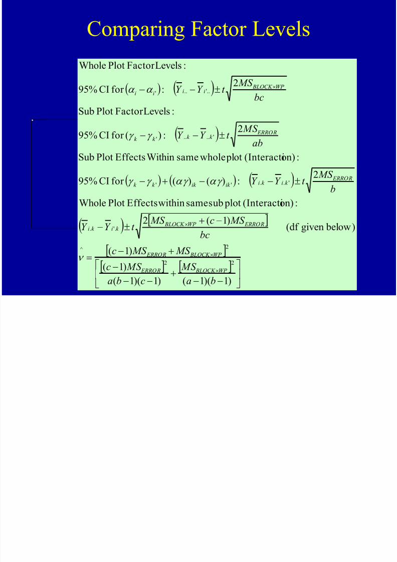
8/14/2019 expdesign.ppt
http://slidepdf.com/reader/full/expdesignppt 76/80
Comparing Factor Levels
)1)(1()1)(1(
)1(
)1(
below)given(df )1(2
:on)(Interacti plotsubsamewithinEffectsPlotWhole
2:)()(forCI%95
:on)(Interacti plotwholesameWithinEffectsPlotSub
2:)(forCI%95
:LevelsFactorPlotSub
2:forCI%95
:LevelsFactorPlotWhole
22
2^
'..
'..''
'....'
'....'
ba
MS
cba
MS c
MS MS c
bc
MS c MS t Y Y
b
MS t Y Y
ab
MS t Y Y
bc
MS t Y Y
WP BLOCK ERROR
WP BLOCK ERROR
ERRO RWP BLOCK k ik i
ERRORk ik iik ik k k
ERRORk k k k
WP BLOCK iiii
Repeated Meas res Designs

8/14/2019 expdesign.ppt
http://slidepdf.com/reader/full/expdesignppt 77/80
Repeated Measures Designs
• a Treatments/Conditions to compare• N subjects to be included in study (each subject
will receive only one treatment)
– n subjects receive trt i: an = N • t time periods of data will be obtained
• Effects of trt, time and trtxtime interaction of
primary interest. – Between Subject Factor: Treatment
– Within Subject Factors: Time, TrtxTime
Model

8/14/2019 expdesign.ppt
http://slidepdf.com/reader/full/expdesignppt 78/80
Model
2
11
1
2
)()(
1
)(
,0~ error termrandom
0)()( timeandt between tr ninteractio)(
0 periodtimeof effect
,0~in trtsubjectof effect
0trtof effect
meanoverall
)(
s
t t t
t t
s
t t
NID
k i
k
NIDbi jb
i
bY
ijk ijk
t
k
ik
a
i
ik ik
t
k
k
th
k
bi j
th
i j
a
i
ii
ijk ik k i jiijk
Note the random error term is actually the interaction between
subjects (within treatments) and time
T t f Fi d Eff t

8/14/2019 expdesign.ppt
http://slidepdf.com/reader/full/expdesignppt 79/80
Tests for Fixed Effects
)~|(
:StatisticTest
,0)(: :nInteractioTimeTreatment/
)~|(
:StatisticTest
0: :EffectsTime
)~|(
:StatisticTest
0: :EffectsTreatment
)1)(1(),1)(1(
0
)1)(1(,1
10
)1(,1
)(
10
t nat aTIME TRT TIME TRT
ERROR
TIME TRT TIME TRT
ik
t nat TIME TIME
ERROR
TIME TIME
t
naaTRTS TRTS
TRTS SUBJECTS
TRTS TRTS
a
F F F F P P
MS
MS F
k i H
F F F F P P
MS
MS F
H
F F F F P P
MS MS F
H
t
t t
C i F t L l

8/14/2019 expdesign.ppt
http://slidepdf.com/reader/full/expdesignppt 80/80
Comparing Factor Levels
)1(
)1(
:df eapproximatwith
)1(2
:LevelsTimeWithinLevelsTreatmentComparing
2:forCI%95
:LevelsTimeComparing
2:forCI%95
:LevelsTreatmentComparing
2
)(2
2
)(^
)('..
'....'k
)('....'
MS MS t
MS MS t
nt
MS t MS t Y Y
an
MS t Y Y
nt
MS t Y Y
TRT SUBJECT ERROR
TRT SUBJECT ERROR
ERRORTRTS SUBJECTS k ik i
ERRORk k
k
TRTS SUBJECTS iiii
t t