1

Exchange Rate, Expected Profit, and Capital Stock Adjustment: *

Japanese Experience

Yoichi Matsubayashi

Graduate School of Economics

Kobe University

Abstract

This paper empirically investigates the impact of exchange rate shocks on corporate investment.

An intertemporal optimization model is developed in which an individual corporation in an open

economy adjusts its capital stock according to the Tobin’s q, which represents the future stream

of the profit rate and changes by the real exchange rate. By explicitly considering the marginal q,

the transmission mechanism from real exchange rate shocks to investment dynamics via expected

profitability is examined based on the Vector Autoregressive model. Empirical evidence suggests

that the depreciation of the Japanese yen increases the expected profitability of the firm and

stimulates corporate investment, especially in the machinery sector. This characteristic basically

corresponds to the structure of external exposure and offers an important finding from the

viewpoint of Japanese macroeconomic fluctuations.

Keywords: Intertemporal Optimization, Marginal q, Pass­Through, Export Exposure

JEL classification number: F40, E22, C32

Please send correspondence to:

Yoichi Matsubayashi Ph.D,

Graduate School of Economics, Kobe University

Rokkodai, Nada­Ku, Kobe, 657­8501, Japan

TEL. +081­78­803­6852

E­mail myoichi@econ.kobe­u.ac.jp

* This paper is a revision of a paper presented at the Moneta ry Economics Seminar (Kobe Univer sity) , 8

December 2007 and at the Annual Meeting of the Japanese Economic Association (Tohoku University), 31 may 2008. I

would like to thank Ryuzo Miyao , Kentaro Iwatasubo (Kobe University), Kazuo Ogawa (Osaka University), Etsuro

Shioji (Hitotsubashi University), Mariko Hatase, Kou Nakayama, Ichiro Muto (Bank of Japan) for their helpful comments

and suggestions. This research was partially supported by the Ministry of Education, Science, Sports, and Culture;

Grant­in Aid for Scientific Research (C) 19530207.

2

1. Introduction In 1973, the Japanese currency switched from a fixed exchange rate, pegged at 360 yen to

the U.S. dollar, to a floating exchange rate. Since then, the yen has appreciated its current high

level and has experienced wide fluctuations with the U.S. dollar. Today, the yen–U.S. dollar

fluctuations are the most volatile among foreign currency pairs 1) . On September 22, 1985, a

Group of 5 developed countries (G5) agreed on the depreciation of the U.S. dollar in the “Plaza

Accord.” After this agreement, the yen appreciated sharply inducing a decline in Japanese

exports. This was cited as the major factor behind the 1986 recession. Until then, Japanese

economic growth had been export­oriented. As a result, in 1985, the existing economic

mechanism started to buckle under the rapid appreciation of the yen. Some Japanese firms began

shifting their production bases overseas where production costs were relatively cheap. This was

the beginning of the exodus of production facilities overseas and has been called the “hollowing

out of industry.” The increase of overseas production has reaccelerated since 2000.

Although there have been large exchange rate fluctuations since the introduction of the

floating exchange rate system, there remain theoretical and empirical questions on the

implications of these movements for real economic activity, especially equipment investment.

Generally speaking, investment plays a central role in both the growth of and fluctuations in the

macroeconomy. In an open economy like Japan, however, it seems that external shocks, such as

the rapid appreciation of the yen, have notable effects on equipment investment.

In a small number of theoretical literatures, Brock (1988) incorporated traded and

non­traded investment into the infinite­horizon optimizing model. By including the non­tradable

sector, he emphasized the endogenous determination of the relative prices of non­traded goods,

referred to as the real exchange rate. Murphy (1993) analyzed the dynamics of the real exchange

rate and equity prices for a small open economy based on the intertemporal optimizing model.

Japanese empirical research focusing on the impact of exchange rate shocks on corporate

investment has been seen in increasing numbers since the end of the 1980s, when the yen began

to appreciate 2) . Tokui and Suzuki (1990) estimated the reduced form between the real exchange

rate and equipment investment in the Japanese machinery sector. Their empirical results showed

significant negative effects of exchange rate appreciation on investment. Tokui and Miyagawa

(1991) constructed the imperfect competitive static model and induced an analytical relationship

between exchange rate and investment. They followed this with several empirical investigations

and their study undertook several important steps. Eichengreen and Hatase (2005) applied the

1) This finding is also discussed in Bank of Japan(2000)/ 2) Miyagawa (1997) made a comprehensive survey in this area. It is worth noting that if investment is affected by the real exchange rate, the framework of the neoclassical saving­investment balance approach, in which investment and saving are not influenced by the real exchange rate, may be modified. The detailed explanation of this point is summarized in Matsubayashi (2006).

3

theoretical framework developed in Tokui and Miyagawa (1991) to investigate whether the real

effective exchange rate had a negative impact on Japanese investment during the fixed exchange

rate system in Japan. Miyagawa and Takeda (1994) extended Brock (1988) and Murphy (1993) to

incorporate the discontinuous adjustment cost of investment. Although the model developed in

their study determines the real exchange rate and investment endogenously, it does not directly

investigate the relationship between the real exchange rate and investment. Its main focus is on

capital accumulation in the trade balance, especially discontinuous adjustment costs. Nonetheless,

their study was the first research to pay substantial attention to the effect of the real exchange rate

on expected profitability.

Outside Japan, only a few attempts have been made. Goldberg (1993) investigated the

linkage between exchange rate and investment in the U.S. He found that the depreciation of the

U.S. dollar stimulated capital stock adjustment during the 1970s. Campa and Goldberg (1995)

introduced a new measure of external exposure, which emphasized the exposure to external

markets through both export sales and import inputs into production, and used this measure to

explore the linkage between exchange rate and investment in the U.S. Campa and Goldberg

(1999) extended these results and estimated their model for the two­digit manufacturing sectors

of the U.S., the U.K., Canada, and Japan. They found that exchange rates tended to have

insignificant effects on investment rates in high markup sectors. On the other hand, the response

of investment to the exchange rate was strong in low markup sectors. Moreover, there was no

significant effect for either low or high markup industries in Canada.

Nucci and Pozzolo (2001) investigated investment responsiveness to exchange rate

fluctuations using firm­level panel data in the Italian manufacturing industry. Their results

support the view that a depreciation of the exchange rate has a positive effect on investment

through the revenue channel and a negative effect through the cost channel.

Harchaoui et al. (2005) examined the relationship between exchange rate and investment

using industry level data for Canadian industries. They showed that the overall effect of exchange

rates on total investment is insignificant. Their investigation also revealed that exchange rate

depreciation had a positive effect on total investment when exchange rate volatility is low.

Based on the above studies, this paper re­examines the impact of exchange rate shocks on

corporate investment. Here there are three distinct analytical differences from earlier studies.

First, an intertemporal optimization model is developed in which an individual corporation in an

open economy adjusts its capital stock according to Tobin’s q under imperfect competition. In

addition, there now exists the development of the New Open Economy Macroeconomics. The

emphasis of this new direction is on the pricing to market (PTM) behavior and on the

pass­through of the exchange rate into export and import prices under imperfect competitive

markets. In pioneering works, Campa and Goldberg (1995, 1999) derived a theoretical derivation

4

of the exchange rate–investment relationship under imperfect competition and investigated it

empirically. Although their studies may have provided an attractive direction for future research,

it did not explicitly consider Tobin’s q, which is a main determinant of investment decisions.

Schiantarelli and Geogoutsos (1990) and Ogawa and Kitasaka (1999) are examples of the

approach that estimates the Tobin’s q type investment function under the assumption that the

product market is imperfectly competitive. This paper constructs the theoretical relationship

between Tobin’s q and investment in an open economy with imperfect competition.

Second, we calculate a series of marginal q in twelve industries with a time series analysis.

Abel and Blanchard (1986) and Ogawa and Kitasaka (1999) have already specified the stochastic

structure underlying the discount factor and profit rate and constructed a series of marginal q.

The approach in this paper follows basically the same track. By explicitly considering the

marginal q in an open economy model, this paper examines the transmission mechanism from

real exchange rate shocks to investment dynamics via expected profit (not present profit) based

on the Vector Autoregressive model (VAR). Accordingly, if the real exchange rate shocks become

more persistent, then more careful investment decisions must be made. This means that these

features are essentially dynamic. Since little attention has been paid to this point, the empirical

methodology adopted in this paper is attractive and actually produces some interesting results.

Third, this model is able to shed light on how investment sensitivity varies across industries.

In this paper, we consider two main factors: export exposure and pricing power. In general,

export­oriented firms are more likely to be affected by exchange rate fluctuations, because the

direct effect on export revenue is greater than the substitution effect in the domestic market. The

second feature is related to the degree of monopoly power, which is proxied by the

price­over­cost markup ratio. When the exchange rate effects on product demand are identical in

high and low markup industries, high­markup firms will dampen the exchange rate effect on

profitability by adjusting their output prices and markups. Therefore, the lower the industry

markup ratio, the stronger the exchange rate effect on profits, and hence on investment.

The remainder of this paper is organized as follows. In Section 2, the basic framework of

this analysis is presented. In Section 3, a data series is calculated. In Section 4, the VAR system is

employed and dynamic simulations are performed. In Section 5, the structures of external

exposure are carefully examined. Finally, In Section 6, our conclusions are presented.

2. Model This section extends the open economy model developed by Campa and Goldberg (1995),

(1999), and Nucci and Pozzolo (2001), in that both input and output prices are affected by the

exchange rate. A representative firm produces one output for the domestic and foreign market

with three types of inputs: quasi­fixed capital (K ), domestic variable input (L ), and foreign

5

variable input ( * L ). The firm maximizes the expected present value of the discounted sum of future dividend (D ) subject to a capital stock accumulation defined as follows:

= ∑

∞

= + +

0 j j t j t t t D E V β (1)

( ) t t t I K K + − = −1 1 δ (2)

( ) j t j t I j t j t

I j t j t j t K I G p I p X D + + + + + + + − − = , (3)

( ) ( ) * * * * * , , j t j t j t j t j t j t j t j t j t j t j t j t L w e L w q e q p q e q p X + + + + + + + + + + + + − − + = (4)

( ) 1

1

1 −

= + + ∏ + =

j

i i t j t r β ,.... 2 , 1 = j 1 ≡ t β

j t D + , net cash flow;

j t X + , total revenue;

j t I + , equipment investment;

( ) j t j t K I G + + , , adjustment costs in changing the capital stock;

j t K + , capital stock at the end of t + j;

I j t p + , price of investment good (deflated by general price index);

1 + t r , one period discount rate in period t;

j t p + , price of good in the domestic market (deflated by general price index);

* j t p + , price of good in the foreign market (deflated by general foreign price index);

j t q + , quantities supplied by the firm to the domestic market;

* j t q + , quantities supplied by the firm to the foreign market;

j t L + , quantities of domestic variable input;

6

* j t L + , quantities of foreign variable input;

j t w + , unit cost of the domestic inputs (deflated by general price index);

* j t w + , unit cost of the foreign inputs (deflated by general foreign price index);

j t e + , real exchange rate defined in terms of domestic currency per unit of foreign exchange

(deflated by general price index in domestic and foreign markets);

δ , physical depreciation rate; and

[ ] t E , conditional expectation operator upon the information available in period t.

Following the standard formation in the investment model (see Hayashi (1982)), it is assumed

that there are convex costs in adjusting the capital stock. The cost of adjustment function is linear

homogeneous in investment ( I ) and capital stock (K ). It is specified as follows:

( )

=

2

2

2 ,

K I

K I G t t t

φ (5)

The firm produces output for both domestic and foreign markets by constant returns to scale

production ( ) ( F )

( ) * * , , t t t t t L L K F q q = + (6)

In equation (4), ) (⋅ p and ) ( * ⋅ p are the domestic and foreign demand curves facing the

firm. These functions depend on both the quantities supplied by the firm to each market and the

exchange rate. The exchange rate directly influences prices because fluctuations in the exchange

rate alter the demand for the firm’s products due to changes in the number of competitors in both

domestic and foreign markets.

Maximizing Equation (1) subject to Equation (3) yields the following conditions:

( ) ( ) * 1 1 *

1 1 t t t p e p − − − = − η η (7)

( ) ( ) * 1 1 *

1 1 t t t p e p − − − = − η η (8)

( ) * * 1 * * 1 t t L t w e F p t

= − − η (9)

7

− = 1 1

I t

t

t

t

p K I λ

φ (10)

( )

+ − =

+

+ +

∞

= + + ∑

2

0 2 1

j t

j t I j t K

j

j j t t t K

I p X E

j t

φ δ β λ (11)

Equation (7) shows that marginal revenue from the domestic market equals marginal

revenue from the foreign market. Equations (8) and (9) state that the marginal cost of domestic

and foreign variable inputs equals the value of their marginal productivities. t λ is the Lagrange

multiplier associated with the above optimization. Equation (10) indicates that the investment is

positive when λ exceeds 1. Equation (11) represents that q is the discounted stream of the future

marginal profit of capital stock, and the discounted stream of its marginal contributions to the

reduction in future adjustment costs.

After some modification, Equation (11) is rewritten as follows:

( ) ( )

( ) ( )

− +

− −

− −

− =

∑ ∑

∑ ∑

∞

= +

+ + +

∞

= +

+ + + −

+

∞

= +

+ + − +

∞

= + +

0

2

0

* * * 1 *

0

1

0

2 1 1

1 1

j j t

j t I j t

j j t t

j j t

j t j t j t j j t t

j j t

j t j t j j t t

j j t

j j t t t

K I

p E K

q p e E

K q p

E E

φ δ β η δ β

η δ β π δ β λ

(12)

j t

j t j t j t j t j t j t j t j t j t j t j t K

L w e L w q p e q p

+

+ + + + + + + + + + +

− − + =

* * * *

π (13)

The economic implication of λ is shown in Equation (12). The first term on the right hand

side is the discounted stream of future profit rate. The fourth term is the discounted stream of its

marginal contributions to the reduction in future adjustment costs. The second and third terms

capture the discounted stream of future monopolistic rent.

Monopolistic rent is regarded as the distortional factor arising from profit under imperfect

competition. In the case of perfect competition in the domestic and foreign market, the price

elasticities of demand (η and * η ) are infinite, and therefore monopolistic rents disappear. As shown in Equation (12), the economic implication of q in the open macroeconomy with

imperfect competition is more complicated than in the standard formation. To avoid complexity

in the discussion below, we concentrate on the movements of the first term of Equation (12).

We take the Taylor expansion around the mean level of the real exchange rate (e ) in Equation (8). The first term on the right hand side in Equation (12) is expressed as follows 3) .

3) * shows that the expansion term is evaluated by the mean level.

8

( ) ( ) ( ) ( ) ( ) e e e

E e E E i t i j j t

j t j j t

i t

j

j j t t

j j t

j j t t −

∂

∂ − +

− ≅

− +

∞

= +

+ +

∞

=

∞

= +

∞

= + + ∑ ∑ ∑ ∑

* 0 0 0

1 1 1 π

δ β π δ β π δ β (14)

In the case of i = 0, Equation (14) is rewritten as

( ) ( ) e e e e

e E t

j t

j t

j t

j t j t j t t −

∂

∂

∂

∂ − ∑

∞

=

+

+

+ + +

* 0

1 π

δ β (15)

In Equation (15), t j t e e ∂ ∂ + indicates the persistency effect and it depends on the time

series property of t e 4) . j t j t e + + ∂ ∂π shows the profit effect and its sign can be identified by

the partial difference by j t e + in Equation (15). First, the time series property of t e is specified

by the following autoregressive process:

∑=

− + + = m

k t k t k t e b b e

1 0 ε (16)

( ) ( ) 2 2 1 1 , 0 σ ε ε = = − − t t t t E E

Equation (16) is expressed by matrix representation as follows:

t t t MD D ξ θ + + = −1 (17)

( ) 1 1 ' ,....., , + − − = k t t t t e e e D

( ) 0 ,....., 0 , 0 ' b = θ

( ) 0 ,....., 0 , ' '

t t ε ξ =

=

0 1 ... 0 0 .. 1 . 0 ... 0 1

... 2 1 k b b b

M

By forward recursive substitution and some modifications, Equation (17) is written as

4) The case of i = 0 is taken to simplify the analysis.

9

( ) ( ) j t t j

t j

t j

j t M M c M I c D M c e + + −

+ −

+ + + + + − + = ε ε ε θ .... 2 2

1 1 ' ' ' (18)

( ) 0 ,....., 0 , 1 ' = c

Then the persistency effect is calculated with Equation (18).

c M c e e j

t

j t ' = ∂

∂ + (19)

The above magnitude can be measured numerically if the stochastic process expressed by

Equation (16) is estimated and the parameter estimates are correctly obtained.

Substituting Equation (19) into Equation (15) with some additional modifications yields the

following formulation:

( ) ( ) ( )

( ) ( )

+ −

∂

∂ − +

− ≅

−

∑ ∑ ∑

∑ ∑ −

= − +

∞

= +

+ +

∞

=

∞

= +

∞

= + +

1

0

' ' '

*

'

0

0 0

1

1 1

i

s s i t

i t

i

i j

j

j t

j t j j t

i t

j

j j t t

j j t

j j t t

M c D D M c c M c e

E

e E E

ξ π

δ β

π δ β π δ β (20)

( ) ( ) [ ] ( ) [ ] θµ η η η ω η η η ω π

− − − − + − − − = ∂

∂

+

+ e MKUP p q e p e MKUP p q e p

j t

j t A e . . . . . . * * * * 1 1 1 1 , (21)

where

TR q ep * *

= ω : share of total revenues associated with foreign sales;

TR L ew wL * * +

= θ : share of total costs associated with total revenues;

* * L ew wL ewL +

= µ : share of imported inputs in total production costs;

p e

e p

e p ∂ ∂

= . η : exchange rate elasticity of price in the domestic market;

*

*

. *

p e

e p

e p ∂ ∂

− = η : exchange rate elasticity of price in the foreign market;

q p

p q

p q ∂ ∂

− = . η : price elasticity of demand in the domestic market;

*

*

*

*

. * *

q p

p q

p q ∂ ∂

− = η : price elasticity of demand in the foreign market;

( ) 1

1

. −

−

∂ ∂

− = MKUP

e e

MKUP e MKUP η : exchange rate elasticity of markup in the domestic

market;

10

( ) 1 *

1 *

. * −

−

∂ ∂

− = MKUP

e e

MKUP e MKUP

η : exchange rate elasticity of markup in the foreign

market.

1 1 1 − − − = η MKUP 1 1 * *

1 − − − = η MKUP

eK TR A =

Based on Equations (20) and (21), there seem to be three main channels by which the

fluctuations of the real exchange rate affect capital stock adjustment. First, if exchange rate

fluctuations persist over the long run, an increase of t e in period t may affect the real exchange

rate in t + j ( j t e + ). We call this effect the “persistency effect.” The size of the persistency effect

is captured by c M c j ' in Equation (20).

Second, the export and import structure will affect the profitability of firms, and therefore

affect investment. We call this the “trade structure effect.” In general, export­oriented firms are

more likely to be affected by exchange rate movements, because the direct valuation effect on

export revenue is greater than the substitution effect in the domestic market. The size of this

effect is given byω , which is the share of total revenues associated with foreign sales. On the other hand, the higher the share of imported inputs in total production costs (µ ), the larger the

increase in the negative effect when the exchange rate depreciates. Moreover, this effect is

amplified by the share of total costs associated with total revenues (θ ). Therefore, the trade effect consists of µ and θ . Third, the degree of the firm’s monopoly power contributes to determining the effect of

exchange rate change on profitability and investment. We call this the “monopoly power effect.”

When focusing on Equation (21), the monopoly power effect is determined by the exchange rate

elasticity of price in the domestic market ( e p. η ), the exchange rate elasticity of price in the

foreign market ( e p . * η ), the exchange rate elasticity of markup in the domestic market ( e MKUP . η ),

and the exchange rate elasticity of markup in the foreign market ( e MKUP . * η ). Here we consider

the case in which the exchange rate appreciates (the value of e decreases). The appreciation of the exchange rate increases the price at the same rate in the foreign market (this means that

e p . * η > 0 ). At first, the price increase revenue ( * * q p ) in the foreign market rises. Therefore,

the profit rate will not decrease at the same rate as the exchange rate appreciation. However, the

rise of price in the foreign market gradually decreases the foreign demand (the absolute value of

11

reduction is measured by e p . * η

e p . * η * * q .p × η ) and the appreciation of the exchange rate reduces

the profit rate. Therefore, if the value of * * .p q η is provided, then the greater is the

e p . * η , the

smaller is e ∂ ∂π . When firms have monopolistic power in the foreign market, they do not

perfectly pass through the change in the exchange rate into the price in the foreign market, and

e p . * η is relatively low. In that case, e ∂ ∂π is smaller than in the case of perfect pass­through.

Next we focus on the parameter e MKUP . * η . Monopolistic power is commonly proxied by the

price­over­cost markup ratio. In an oligopolic market structure with a high markup ratio, firms

will dampen the exchange rate effect on profitability by adjusting markups. In contrast, in highly

competitive industries, firms have very limited pricing power and prices are set near the marginal

cost (hence e MKUP . * η is small). Therefore, adjustments to exchange rates are largely reflected in

changes in the firm’s profit. To sum up, the lower the industry markup ratio in the foreign market,

the stronger the exchange rate effect on profitability, and hence on investment 5) .

Taking into account the above analytical considerations, an appreciation of the real exchange

rate may decrease investments, but this cannot be recognized precisely. Therefore, detailed

empirical examinations are indispensable in the following sections.

3.Data The main variables in this study are the investment­capital ratio, the real exchange rate, and

the marginal q. This section introduces how these variables are calculated 6) .

The above theoretical model assumes that corporate investments consist of only

non­residential buildings and structures. In fact, this data is chosen from the Quarterly Report of

Financial Statements of Incorporated Business (compiled by the Ministry of Finance). Twelve

industries are selected over the period from 1975 (Q1) to 2005 (Q4). They comprise chemicals,

steel, nonferrous metals, fabricated metals, industrial machinery, transportation machinery,

electrical machinery, precision machinery, wholesale, construction, and electricity. The sample

period basically corresponds to the period of the floating exchange rate regime in which there

have been remarkable exchange rate fluctuations for about thirty years.

Table 1 summarizes the basic statistics on the investment­capital ratio in each industry. The

average value of the machinery sector is larger than that of the materials sectors and

5) In this situation, firms reduce the markup ratio and do not change the price. Krugman (1987) calls this phenomenon “pricing to market” (PTM). 6) The details of the calculations are provided in the Appendix.

12

non­manufacturing industries. This finding shows that the investments in the value­added

industries represented by precision machinery and electrical machinery are relatively high 7) . The

volatility measured by the coefficient of the variation differs from industry to industry. The steel

industry and construction industry, in which investments are large, each adjust their capital stock

frequently.

The exchange rate is the real effective exchange rate as computed by the Bank of Japan. The

marginal q is unobservable since it includes unobservable factors such as the future stream of the

profits rate and a subjective discount factor. Since the discounted value of the marginal

adjustment costs (the fourth term of Equation (12)) seems to be relatively small, this term is

ignored. The discounted value of monopolistic rent (the second and third terms of Equation (12))

is also ignored. Then equation (12) is rewritten as follows:

( )

− = ∑

∞

= + +

0 1 1

j j t

j j t t I

t t E

p Mq π δ β (22)

To make Equation (22) operational, one has to know the stochastic structure underlying the

profit rate and discount factor. Ogawa and Kitasaka (1999) constructed a series of marginal q

based on the univariate autoregressive specification of the underlying factors 8) . The approach in

this paper is basically on the same track except for the specification of the stochastic process

underlying the two variables. Unlike Ogawa and Kitasaka (1999), we conduct a multivariate

autoregressive specification because the profit rate and discount factor, which are calculated by

the required interest, may simultaneously determine that they are affected by each other 9) . Before

specification, the unit root and cointegration test are conducted on both variables. In almost

industries, profit rate and discount factor are nonstationary, and a cointegration relationship

between them is not observed. Then the stochastic process for profit rates and discount factor is

specified as in the following VAR model:

t i t

k

i i i t

k

i i t b d b b d 1

1 2

1 1 10 ε π + ∆ + ∆ + = ∆ −

= −

= ∑ ∑ (23)

t i t

k

i i i t

k

i i t b d b b 2

1 4

1 3 20 ε π π + ∆ + ∆ + = ∆ −

= −

= ∑ ∑ (24)

7) In the 1960s, however, construction investments in materials industries were high, and the Japanese business cycles in the period were induced by the demand for construction. See Yoshikawa (1995) for the details. 8) Ogawa and Kitasaka (1999) estimated the investment function in the Japanese manufacturing industry over the period from 1970 Q1 to 1990 Q4. 9) Ogawa (2000) and Otaki and Suzuki (1986) specify the stochastic process as bivariate­VAR.

13

t t r d

+ −

= 1 1 δ

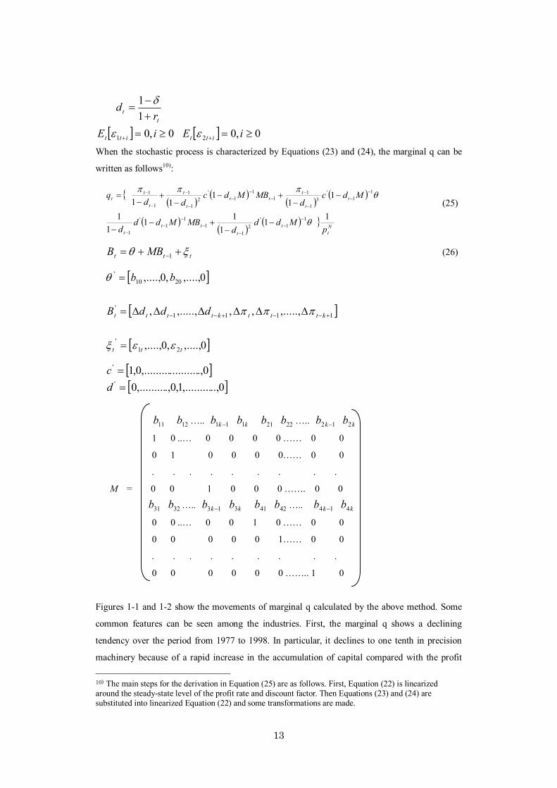
[ ] 0 , 0 1 ≥ = + i E i t t ε [ ] 0 , 0 2 ≥ = + i E i t t ε When the stochastic process is characterized by Equations (23) and (24), the marginal q can be

written as follows 10) :

( )

( ) ( )

( )

( ) ( )

( ) N t

t t

t t t

t t

t t t

t

t

t

t t

p M d d

d MB M d d

d

M d c d

MB M d c d d

q

1 1 1

1 1 1

1

1 1

1 1 1

1 1

' 2

1 1

1 1

'

1

1 1

' 3

1

1 1

1 1

' 2

1

1

1

1

θ

θ π π π

− −

− −

− −

−

− −

−

− −

− −

−

−

−

−

− −

+ − −

− −

+ − −

+ −

= (25)

t t t MB B ξ θ + + = −1 (26)

[ ] 0 ,...., , 0 ,...., 20 10 ' b b = θ

[ ] 1 1 1 1 ' ,....., , , ,....., , + − − + − − ∆ ∆ ∆ ∆ ∆ ∆ = k t t t k t t t t d d d B π π π

[ ] 0 ,...., , 0 ,...., 2 1 '

t t t ε ε ξ =

[ ] 0 ., .......... ,......... 0 , 1 ' = c [ ] 0 .., ,......... 1 , 0 ., ,......... 0 ' = d

11 b 12 b ….. 1 1 − k b k b 1 21 b 22 b ….. 1 2 − k b k b 2 1 0 ..… 0 0 0 0 …… 0 0

0 1 0 0 0 0…… 0 0

. . . . . . . . .

M = 0 0 1 0 0 0 ……. 0 0

31 b 32 b ….. 1 3 − k b k b 3 41 b 42 b ….. 1 4 − k b k b 4 0 0 ..… 0 0 1 0 …… 0 0

0 0 0 0 0 1…… 0 0

. . . . . . . . .

0 0 0 0 0 0 …….. 1 0

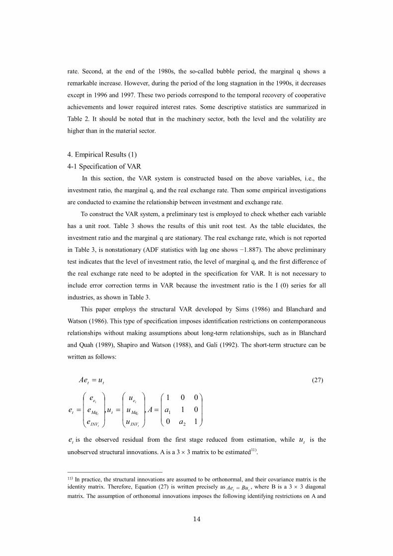
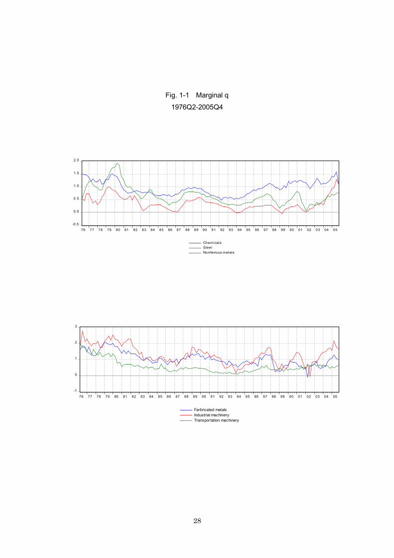
Figures 1­1 and 1­2 show the movements of marginal q calculated by the above method. Some

common features can be seen among the industries. First, the marginal q shows a declining

tendency over the period from 1977 to 1998. In particular, it declines to one tenth in precision

machinery because of a rapid increase in the accumulation of capital compared with the profit

10) The main steps for the derivation in Equation (25) are as follows. First, Equation (22) is linearized around the steady­state level of the profit rate and discount factor. Then Equations (23) and (24) are substituted into linearized Equation (22) and some transformations are made.

14

rate. Second, at the end of the 1980s, the so­called bubble period, the marginal q shows a

remarkable increase. However, during the period of the long stagnation in the 1990s, it decreases

except in 1996 and 1997. These two periods correspond to the temporal recovery of cooperative

achievements and lower required interest rates. Some descriptive statistics are summarized in

Table 2. It should be noted that in the machinery sector, both the level and the volatility are

higher than in the material sector.

4. Empirical Results (1) 4­1 Specification of VAR

In this section, the VAR system is constructed based on the above variables, i.e., the

investment ratio, the marginal q, and the real exchange rate. Then some empirical investigations

are conducted to examine the relationship between investment and exchange rate.

To construct the VAR system, a preliminary test is employed to check whether each variable

has a unit root. Table 3 shows the results of this unit root test. As the table elucidates, the

investment ratio and the marginal q are stationary. The real exchange rate, which is not reported

in Table 3, is nonstationary (ADF statistics with lag one shows −1.887). The above preliminary

test indicates that the level of investment ratio, the level of marginal q, and the first difference of

the real exchange rate need to be adopted in the specification for VAR. It is not necessary to

include error correction terms in VAR because the investment ratio is the I (0) series for all

industries, as shown in Table 3.

This paper employs the structural VAR developed by Sims (1986) and Blanchard and

Watson (1986). This type of specification imposes identification restrictions on contemporaneous

relationships without making assumptions about long­term relationships, such as in Blanchard

and Quah (1989), Shapiro and Watson (1988), and Gali (1992). The short­term structure can be

written as follows:

t t u Ae = (27)

=

=

= 1 0 0 1 0 0 1

, ,

2

1

a a A

u u u

u e e e

e

t

t

t

t

t

t

INV

Mq

e

t

INV

Mq

e

t

t e is the observed residual from the first stage reduced from estimation, while t u is the

unobserved structural innovations. A is a 3 × 3 matrix to be estimated 11) .

11) In practice, the structural innovations are assumed to be orthonormal, and their covariance matrix is the identity matrix. Therefore, Equation (27) is written precisely as

t t Bu Ae = , where B is a 3 × 3 diagonal matrix. The assumption of orthonomal innovations imposes the following identifying restrictions on A and

15

4­2 Impulse response in VAR Based on the above types of specification, the VAR systems in the individual industries are

estimated and some simulations are employed. It is well known that these simulation results

depend largely on the lag length. To deal with the lag problem, two different types of lag lengths,

two and four, are selected to check the robustness of the simulation results 12) .

In the two specifications of lag length, the simulation results do not differ greatly. Then the

impulse response functions with lag two are reported in Figures 2­1–2­12 to assess the

quantitative impact of a real exchange rate shock. In each case, one standard deviation of

residuals in the real exchange rate equation is generated as a yen depreciation shock, and impulse

responses for periods 0 through 40 (for 10 years) are simulated. Response standard errors are also

computed by Monte Carlo simulation with one thousand repetitions. The first column in each

figure shows the accumulated response of marginal q to an exchange rate shock. The second

column is the accumulated response of marginal q to investment. A real exchange rate shock

influences the investment dynamics via the marginal q. Then, comprehensive considerations are

necessary based on the above two types of accumulated impulses.

Accumulated responses in manufacturing are shown in Figures 2­1–2­9. The effect of a real

exchange rate shock induces a contemporaneous increase in the marginal q; however, this

increase is not necessarily sustained. Investment is stimulated by the exchange rate as shown in

the second column. The accumulated response of investment is significantly positive in almost

manufacturing industries. These simulation results indicate that real exchange rate depreciation

shocks may possibly stimulate investment via the marginal q in manufacturing industries. On the

other hand, in the non­manufacturing sector, the effect of a real exchange rate shock on

investment is almost insignificant.

Figure 3 summarizes the accumulated responses of marginal q and investment to the real

exchange rate calculated in Figure 2. The impact of the yen’s depreciation on the machinery

sectors, especially transportation machinery and industrial machinery, is relatively large.

Interestingly, the accumulated response of marginal q to the real exchange rate for electrical

machinery and precision machinery is relatively weak. The implications of this finding are

investigated carefully in the subsequent section.

B: [ ] ∑ ∑ = = ' ' ' , t t e e E BB A A . 12) To select the lag order of VAR, various criteria, such as the Akaike Information Criterion (AIC), the Shwarz Information Criterion (SBIC), the Hanann­Quinn Criterion (HAC), and other statistical tests, such as Likelihood test have been considered. However, these criteria do not necessarily sign the same lag length. Considering these problems, two types of ad hoc lag lengths are assumed in this paper.

16

5. Empirical Results (2) 5­1 Structure of external exposure

In the previous section, the accumulated responses of marginal q and investment to the real

exchange rate vary in each industry. In general, the magnitude is high in the manufacturing sector.

However, careful observation reveals that the magnitude in the manufacturing industry differs

across sectors. Some examinations are conducted to investigate this point.

The firm’s structure of external exposure is theoretically derived in Equations (20) and (21).

First, the export and import structure will affect the profitability of the firms, and therefore affect

investment. In general, export­oriented firms are more likely to be affected by exchange rate

movements, because the direct valuation effect on export revenue is greater than the substitution

effect in the domestic market. The size of this effect is given byω , which is the share of total revenues associated with foreign sales. Second, the higher the share of imported inputs in total

production costs (µ ), the larger the increase in the negative effect when the exchange rate

depreciates. Moreover, this effect is amplified by the share of total costs associated with total

revenues (θ ). Therefore, the trade effect consists of µ and θ . The values of the above parameters in each industry are summarized in Table 4. It is clear that

the export share is relatively high in the machinery sectors and its average share is about thirty

percent. On the other hand, in the non­manufacturing industries, the export share is nearly zero

percent. The import input share in the material sectors is larger than that of the machinery sectors.

The impact of the yen’s depreciation on the machinery sectors, especially transportation

machinery and industrial machinery, is relatively large. This tendency seems to be consistent with

the high level of the share of exports in total revenues. However, it is unclear why the

accumulated response of marginal q to the real exchange rate for electrical machinery and

precision machinery is relatively weak despite its high export share.

5­2 Structure of oligopolic power The degree of a firm’s monopoly power contributes to determining the effect of exchange

rate change on profitability and investment. We call this effect the “monopoly power effect.”

When focusing on Equation (21), the monopoly power effect is determined by the exchange rate

elasticity of price in the domestic market ( e p. η ), the exchange rate elasticity of price in the

foreign market ( e p . * η ), the exchange rate elasticity of markup in the domestic market ( e MKUP . η ),

and the exchange rate elasticity of markup in foreign market ( e MKUP . * η ). Here we focus on the

17

values of e p . * η and e MKUP . * η . The time­varying estimation of

e p . * η in each industry is shown

in Figure 4 13) . Interestingly, e p . * η in the machinery sectors is lower than in the material sectors.

This implies that the oligopolic power of the machinery sectors is relatively high and that its

pass­through is weak.

Chida (1995) examines the markup ratio for industrial machinery, electric machinery, and

transportation machinery. His contribution is worth mentioning because the calculation is made

in both the domestic and foreign market. Chida (1995) finds that the value of the markup ratio is

higher in the electric machinery than in any other industry. Using the markup value calculated by

Chida (1995), e MKUP . * η is estimated and the result is summarized in Table 6. It is clear that the

markup elasticity is relatively high in the electric machinery, and that such high elasticity will

dampen the exchange rate effect on profit and investment by adjusting markups. The last column

in Table 5 summarizes the total effect on export share (ω ), export price elasticity ( e p . * η ), and

markup elasticity ( e MKUP . * η ). The calculation result indicates that the impact of the exchange

rate on profit differs across the machinery sectors and is relatively small in the electric machinery.

This finding is consistent with the results in Figure 3­1.

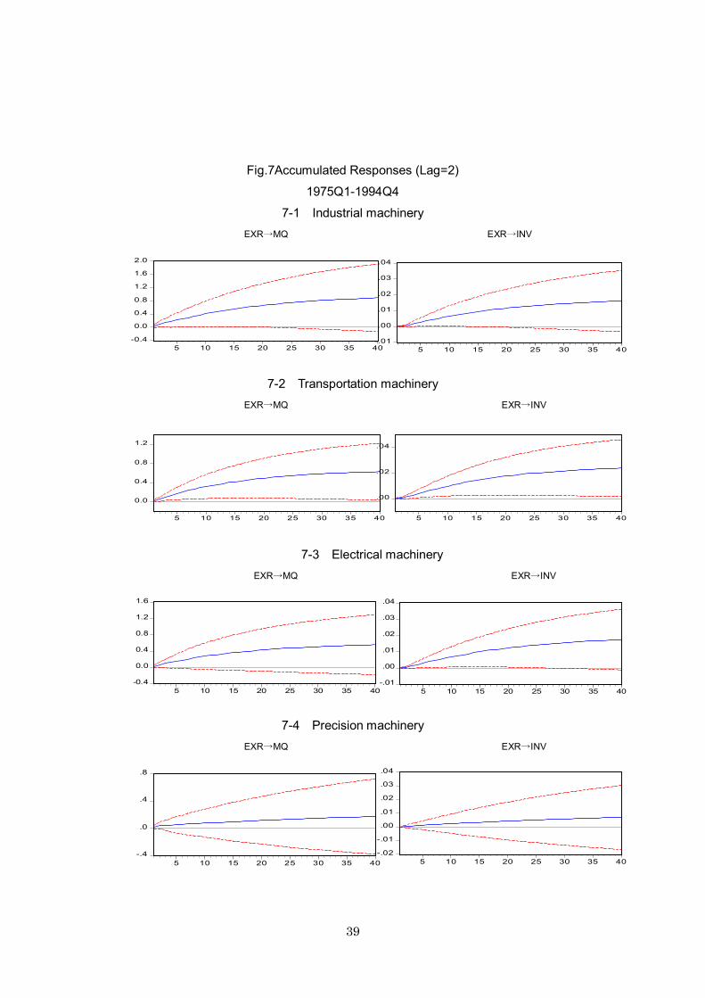
5­3 Persistency of exchange rate movement In the previous section, a series of real exchange rates turned out to be a random walk

process, and this implied that exchange rate shocks are persistent. To examine the persistency

effect, the measure of persistency effect specified in Equation (19) is calculated 14) . Figure 5

shows that the persistency effect declines after the beginning of the 1990s. This is consistent with

the appreciation of the yen from the end of the 1980s to the beginning of the 1990s. These

exchange rate movements have a persistent effect on both profitability and investment. To

examine this point, estimation periods for the VAR system are divided into two sub periods: the

former period is from 1975Q1 to 1994Q4 and the latter is from 1995Q1 to 2005Q4. Impulse

responses are calculated for each period and the simulation results are summarized in Figures 7

and 8. As both figures show, the impulse responses of marginal q and investment to exchange

rate are relatively high in the former periods.

13) Rolling regressions are conducted to estimate e p . * η over the period from 1984Q1 to 2003Q1.

14) The stochastic process of the real exchange rate follows the AR(4) process. Rolling regression is conducted over the period from 1980Q1 to 2005Q4 (estimation windows are 8 years).

18

6. Conclusions There is a lack of both theoretical and empirical literature on the significant impact of

recent exchange rate fluctuations on the real economic activity, especially equipment investment.

This paper has succeeded in theoretically deriving the linkages among the investment, marginal q,

and exchange rate by developing an intertemporal optimization model in which domestic firms

interact with external markets under imperfect competition.

By explicitly considering the marginal q, this paper examines the transmission mechanism

from real exchange rate shocks to investment dynamics via expected profitability is empirically

investigated based on the Vector Autoregression (VAR) model and obtains some interesting

results. In previous literature, little attention was given to dynamic characteristics. In addition,

the empirical methodology adopted in this paper seems attractive. The evidence suggests that the

Japanese yen depreciation has some effect in increasing the expected profitability, and that the

stimulation of investment in the manufacturing industry is larger than that in the

non­manufacturing industry. More careful investigation indicates the following two points. First,

the impact of the yen’s depreciation on the machinery sectors, especially transportation

machinery and general machinery, is relatively large. This tendency seems to be consistent with

the high­level share of export in total revenues. In the case of electric machinery, however, the

impact of the exchange rate on investment is small. This characteristic reflects that the stronger

an industry’s oligopolic power, the lower the exchange effect on profits, and hence on investment.

Second, the magnitude of the implied investment response to exchange rates varies over time

with changes in the permanent component of exchange rates. As this paper shows, since the end

of the 1990s, permanent changes in the Japanese yen have become relatively weak, and thus the

impact of the exchange rate on investment has declined.

Japan’s economy has been expanding moderately since early 2002. The remarkable feature

of today’s economy is that a rise in exports has played the central role in this expansion.

Moreover, Japanese firms have been successful in capturing global demand, as evidenced in this

increase in exports, and this rapid export growth induces corporate investment. Looking at the

real effective rate, it started to fall in 2002. This movement has also affected export growth.

However, the recent export expansion is not merely driven as a consequence of the yen’s

depreciation. Rapid growth in the global economy and the production of higher value­added

export goods also play an important role in recent export expansion. Considering these factors, it

seems that, since 2000, the Yen depreciation has had a strong effect of increasing expected

profitability and also of stimulating investment.

There seem to be some important tasks for future research. The first task is to investigate the

dynamic properties in non­manufacturing sectors more carefully, and to test empirically the

spectral substitution mechanism of economic resources by exchange rate fluctuations. All talks of

19

industrial restructuring, especially prevalent in non­manufacturing sectors, ceased at the end of

the 1980s because Japan entered a short­term economic boom known as the bubble economy.

The second task is to examine the impact of exchange rate uncertainty on the level of

investment. Frequent changes in the exchange rate increase the volatility, and hence uncertainty.

Given the uncertainty, firms often find it convenient to delay investing. Under the floating rate

system, these problems become serious and careful investigations are indispensable.

The last task is to develop a model in which both domestic investment and foreign direct

investment are jointly determined. The increase in overseas production has reaccelerated since

2000, and this tendency now requires research on the capital stock mechanism from an

international perspective.

Data Appendix

The data in this study is taken mainly from the Quarterly Report of Financial Statements of

Incorporated Business compiled by the Ministry of Finance. Seven industries are selected over

the period from 1975 (Q1) to 2005 (Q4): chemicals, steel, nonferrous metals, fabricated metals,

industrial machinery, transportation machinery, electrical machinery, precision machinery,

wholesale, construction, and electricity.

It should be noted that there are discontinuities in the data series in the Quarterly Report of

Financial Statements. A complete renewal of all corporations is conducted every April (Quarterly

one) and the number of corporations is fixed for one year. The Institute for Social Engineering

(1976) and Ogawa (2000) provide detailed procedures for correcting such data discontinuities.

The procedures suggested by them are adopted in this study.

Corporate Investment ( t I ) and Capital Stock ( t K ) Data in investment is given in the Quarterly Report of Financial Statements. Real

investment series are deflated by the price of the construction good reported in the Annual Report

of Prices (Bank of Japan). Given the initial value of the capital stock, real investment series, and

physical depreciation rate, the value of the real capital stock for each industry is computed by the

perpetual inventory method. The physical depreciation rate is given by Ogawa and Kitasaka

(1999), Table A­2. A division of the real investment by the capital stock yields the

investment­capital stock, which is used in this empirical research. Some descriptive statistics for

this series are reported in Table 1.

20

Profit Rates ( t π ) and Discount Factor ( t d ) The marginal q is unobservable since it includes unobservable factors such as the future

stream of the profits rate and the subjective discount factor. Therefore, one has to know the

stochastic structure underlying the profit rate and discount factor.

The profit rate is calculated as the ratio of operating profit to real capital stock computed by

the above procedure. The subjective discount factor consists of the nominal discount rate ( t r ) and the physical depreciation rate. The nominal discount rate ( t r ) is calculated by the following method:

= r r (interest and discount paid + bond interest expenses)/(short­term and long­term loans

payable + bonds payable + notes receivable discounted).

Export Price ( * t p )

Export price is given in export price index (Bank of Japan).

21

References

Abel, A. B. and O. Blanchard (1986) ,"The present value of profits and cyclical movements

in investment," Econometrica, 54, 249­273.

Bank of Japan (2000), “Exchange rate volatility and export behavior,” Bank of Japan Monthly,

March.

Bank of Japan (2007), “Recent development of Japan’s external trade and corporate behavior,”

Bank of Japan Reports & Research Papers, October.

Blanchard, O. J and D. Quah (1989), “The dynamic effects of aggregate demand and supply

disturbances,” American Economic Review, 79, 655­673.

Blanchard, O. J and W. Watson (1986), “Are business cycle all alike ?” in R. Gordon ed.,

The American business cycle: continuity and change, University of Chicago press,

123­179.

Brock, P. L (1988),“Investment, the current account, and the relative price of non­traded

goods in a small open economy,” Journal of International Economics 24, 235­253.

Brock, P. L and S. Turnovsky (1993),“The dependent economy model with both traded and

non­traded capital goods,” NBER Working Paper No.4500.

Campa, J and L. S. Goldberg (1995), “Investment in manufacturing, exchange rates and

external exposure,” Journal of International Economics 38, 297­320.

Campa, J and L. S. Goldberg (1999), “Investment, pass­through and exchange rates: a cross

country comparison.” International Economic Review, 40, 287­314.

Chida, R, (1995), “The export behavior under the imperfect competition,” Economic Bulletin,

Tokyo International University, 13, 19­41.

Clarida, R. H (1997), “The real exchange rate and U.S. manufacturing profits: A theoretical

framework with some empirical support,” International Journal of Finance and

Economics, 2, 177­187.

Darby, J, A, H. Hallet, J. Ireland, and L, Piscitelli, (1999), “The impact of exchange rate

uncertainty on the level of investment,” Economic Journal, 109, 55­67.

Dornbusch, R (1987), “Exchange rates and prices,” American Economic Review, 77, 93­106.

Economic Planning Agency (1995), Annual Report of the Economic Activity.

Eichengreen, B and Mariko Hatase (2005), “Can a Rapidly­Growing Export­Oriented Economy

Smoothly Exit an Exchange Rate Peg? Lessons for China from Japan’s High­Growth

Era,”NBER Working Paper No.11625.

Froot, K and P. Klemperer, (1989), “Exchange rate pass­thorough when market share

matters, ” American Economic Review, 637­654.

22

Gali, J (1992) “How well does the IS­LM model fit postwar U.S. Data ?” Quarterly Journal of

Economics ? 107, 709­738.

Goldberg, L. S (1993) “Exchange rates and investment in United States industry,”

Review of Economics and Statistics 32, 575­588.

Harchaoui, T. F. Tarkhani , and T. Yuen (2005), “The effects of the exchange rate on

investment: evidence from Canadian manufacturing industries,” Bank of Canada

Working paper, 2005­22.

Hayashi, F (1982), “Tobin’s marginal q and average q: a neoclassical interpretation,”

Econometrica, 50, 213­224.

Institute for Social Engineering (1976), Research on advanced use of report of financial

Statements of Incorporated Business.

Knetter, M. M (1989), “Price discrimination by U.S. and German exporters,”

American Economic Review, 79, 198­210.

Knetter, M. M (1993), “International comparisons of pricing­to market behavior,”

American Economic Review, 83, 473­486.

Kruguman, P (1987), “Pricing to market when the exchange rate changes,” Richardson, A ed.,

Real­financial linkages among open economies, MIT press.

Lutkepohl, H (1991), Introduction to multiple time series analysis, Springer­Verlag.

Mackinnon, J. G. (1991), “Critical values for cointegration Tests,” in R. F. Engle and C. W. J.

Granger eds., Long­Run Economic Relationship, Oxford.267­276.

Marston, R. C (1990), “Pricing to market in Japanese manufacturing,” Journal of International

Economics, 29, 217­236.

Marston, R. C (1991), “Price behavior in Japanese and U.S. manufacturing ,” P, R. Kruguman

ed, Trade with Japan: Has the door opened wider ? University of Chicago press.

Matsubayashi, Y (2006), “Structural and cyclical movements of the current account in Japan: an

Alternative Measure ,”Japan and the World Economy, 18, 545­567.

Miyagawa, T (1997), “The development of corporate investment theory and the variety of

empirical study,”Asako, K and M. Otaki ed Macroeconomic Dynamics, Tokyo

University Press.

Miyagawa, T and Y. Takeda (1994), “Investment and the persistence of Japanese trade

surplus,” Japan Center for Economic Research Discussion Paper No.34.

Murphy, R.G (1993),”Stock prices, real exchange rates and optimal capital accumulation,”

IMF Staff Papers 36, 102­129.

Nucci, F and A, F. Pozzolo (2001), “Investment and the exchange rate: An analysis with

firm­level panel data,” European Economic Review, 45, 259­283.

Obstefeld, M and K. Rogoff (1996), Foundations of International MacroeconomicsMIT Press.

23

Ogawa, K and S, Kitasaka (1999), “Market valuation and the q theory of investment,”

Japanese Economic Review, Vol.50, 191­211.

Ogawa, K (2000), “Transmission mechanism of monetary policy,” Osano, H and Y, Honda ed

Modern Finance and Policy, Nihon Hyoronsha.

Osterwald­Lenum, M (1992), “A note with quantiles of the asymptotic distribution of maximum

likelihood cointegrationrRank Test,” Oxford Bulletin of Economics and Statistics,

54, 461­472.

Otaki, M and K. Suzuki (1986), “Tobin’s q and the fluctuations of profit rate and discount

factor,”Kokumin Keizai, 152.

Otani, A., S. Shiratsuka, and T. Shirota, (2003), “The decline in exchange rate pass­through:

evidence from Japanese import prices,”Monetary and Economic Studies, 21, 53­81.

Otani, A., S. Shiratsuka, and T. Shirota, (2005), “ Revisiting the decline in exchange rate

pass­through: further evidence from Japan’s import price,” IMES Discussion paper

series, 2005­E­6.

Schiantarelli, F and D, Georgoutsos, (1990), “Monopolistic competition and the q theory of

investment,” European Economic Review, 34, 1061­1078.

Shapiro, M and M, W. Watson (1988), “Sources of business cycle fluctuations,” NBER

macroeconomic annual.

Sims, C. A (1986), “Are forecasting models usable for policy analysis ?” Quarterly Review 10,

Federal Reserve Bank of Minneapolis, 2­16.

Swift, R, (2006), “Measuring the effects of exchange rate changes on investment in Australian

manufacturing industry,” Economic record, 82, 19­25.

Toda, H (1995), “Finite sample performance of likelihood ratio tests for cointegrating ranks

in vector autoregressions,” Econometric Theory, 11, 1015­1032.

Tokui, J and T. Mityagawa (1991),”Price competitiveness and the investment behavior in

Japanese manufacturing industries,” Japan Development Bank Discussion Paper Series

9105.

Tokui, J and K. Suzuki (1990),”Exchange rate adjustment and international competitiveness

in Japan and U.S.,” Sohichi Kinoshita ed The development of Pacific Rim Countries

and Structural Adjustment Nagoya University Press.

Vigfusson, R. J, N. Sheets, and J. Gagnon, (2007), “Exchnage rate pass­through to export prices:

Assessing some cross­country evidence,” International Finance Discussion Paper,

No.902, Board of Governors of the Federal Reserve System.

Yoshikawa, H (1995), Macroeconomics and the Japanese Economy, Oxford University Press.

24

Table.1 Summary statistics of Investment­Capital Ratio 1975Q1­2005Q4

Industry Mean Standard

Deviation Coefficient of

Variation Maximum Minimum

Total Manufacturing

sector 0.037 0.021 0.573 0.140 0.019

Chemicals 0.036 0.024 0.678 0.163 0.018

Steel 0.032 0.025 0.790 0.159 0.013

Nonferrous metals 0.037 0.021 0.585 0.154 0.019

Fabricated metals 0.037 0.021 0.532 0.114 0.019

Industrial Machinery

0.037 0.020 0.533 0.128 0.019

Transportation Machinery

0.047 0.028 0.594 0.162 0.021

Electrical Machinery

0.039 0.023 0.603 0.161 0.019

Precision Machinery

0.045 0.029 0.642 0.189 0.020

Total Non­ Manufacturing

Sector 0.044 0.032 0.735 0.228 0.018

Wholesale 0.034 0.022 0.662 0.135 0.012

Construction 0.038 0.033 0.860 0.212 0.009

Real estate 0.034 0.020 0.596 0.165 0.011

Electricity 0.036 0.025 0.696 0.135 0.011

25

Table.2 Summary Statistics of of Marginal q 1976Q2­2005Q4

Industry Mean Standard

Deviation Coefficient of Variation

Total Manufacturing

sector 0.842 0.271 0.322

Chemicals 0.946 0.265 0.280

Steel 0.355 0.265 0.746

Nonferrous metals 0.660 0.363 0.549

Fabricated metals 1.022 0.411 0.402

Industrial Machinery

1.269 0.572 0.450

Transportation Machinery

0.555 0.352 0.634

Electrical Machinery

0.892 0.452 0.506

Precision Machinery

1.079 0.647 0.599

Total Non­ Manufacturing

Sector 0.572 0.186 0.325

Wholesale 2.188 0.667 0.304

Construction 1.717 0.468 0.272

Real estate 2.035 0.528 0.259

Electricity 0.548 0.158 0.288

26

Table.3 Unit Root Test 1976Q2­2005Q4

Investment Ratio Marginal q Industry

Drift +Trend Drift Drift +Trend Drift Total

Manufacturing sector

­5.717*** (0)

­7.043*** (0)

­1.440 (4)

­2.317 (4)

Chemistry ­7.132*** (0)

­7.929*** (0)

­1.868 (4)

­1.809 (4)

Steel ­7.820*** (0)

­8.873*** (0)

­2.163 (2)

­2.623* (2)

Nonferrous metals ­5.402*** (0)

­5.226*** (0)

­3.295* (1)

­2.827* (1)

Fabricated metals ­5.163*** (0)

­6.137*** (0)

­2.866 (4)

­2.324 (4)

Industrial Machinery

­3.382*** (0)

­2.662* (0)

­2.692 (0)

­2.598* (0)

Transportation Machinery

­5.652*** (0)

­6.164*** (0)

­2.640 (1)

­3.745*** (1)

Electrical Machinery

­2.606 (0)

­4.790*** (0)

­4.346*** (0)

­3.965*** (0)

Precision Machinery

­4.193*** (0)

­5.118*** (0)

­2.159 (0)

­2.795* (0)

Total Non­ Manufacturing

Sector ­4.496***

(1) ­4.646***

(0) ­1.489

(3) ­2.268

(3)

Wholesale ­1.835 (0)

­3.258** (0)

­3.412* (0)

­3.907** (0)

Construction ­4.214*** (0)

­5.135*** (0)

­2.309 (2)

­2.332 (2)

Real estate ­1.469 (1)

­2.410 (1)

­1.645 (1)

­1.265 (1)

Electricity ­3.279* (2)

­3.746*** (2)

­6.032*** (0)

­4.596*** (0)

ADF test shows augmented Dickey­Fuller test. Optimal lag length determined by Schwarz Information

Criterion is shown in parentheses. * denotes the significance level at the 10% level, ** at the 5% level,

and *** at the 1%

27

Table.4 . Structure of External Exposure（１）

Industry Export share

ω Total cost share

θ

Import input share

µ

Total cost share× Import input share

µ θ ×

Chemicals 0.175 0.682 0.117 0.079

Steel 0.179 0.790 0.070 0.055 Nonferrous metals

0.126 0.870 0.052 0.045 Fabricated metals

0.026 0.798 0.098 0.078 Industrial Machinery 0.265 0.768 0.093 0.071

Transportation Machinery 0.345 0.845 0.032 0.027 Electrical Machinery 0.327 0.834 0.076 0.063 Precision

Machinery 0.367 0.763 0.076 0.052

Wholesale 0120 0.864 NA NA

Construction 0.023 0.837 0.033 0.027

Real estate 0 0.555 NA NA

Electricity 0 0.739 0.184 0.139

Export share in 2005 is from Short­term Economic Survey of Enterprises in Japan (BOJ). Total input

share in 2005 is from Quarterly Report of Financial Statements of Incorporated Business (compiled by the Ministry of

Finance). Import input share in 2000 is from Asian international Input­output Table (Asian International input­output

Project Institute of Developing Economies Japan External Trade Organization)

Table.5. Structure of External Exposure（２）

Industry Export share

ω

Export price

elasticity

e p . * η

Markup elasticity

e MKUP . * η

Export volume elasticity

e p p q . . * * * η η ×

Total effect

( ) e MKUP p q e p e p . . . . * * * * * 1 η η η η ω − × + −

Industrial Machinery 0.265 0.120 0.593 0.484 0.204

Transportation Machinery 0.345 0.155 0.602 0.489 0.252 Electrical Machinery 0.327 0.126 0.759 0.475 0.192

28

Fig. 1­1 Marginal q

1976Q2­2005Q4

­0.5

0.0

0.5

1.0

1.5

2.0

76 77 78 79 80 81 82 83 84 85 86 87 88 89 90 91 92 93 94 95 96 97 98 99 00 01 02 03 04 05

Chemicals Steel Nonferrous metals

­1

0

1

2

3

76 77 78 79 80 81 82 83 84 85 86 87 88 89 90 91 92 93 94 95 96 97 98 99 00 01 02 03 04 05

Farbricated metals Industrial machinery Transportation machinery

29

Fig. 1­2 Marginal q

1976Q2­2005Q4

­1

0

1

2

3

4

5

76 77 78 79 80 81 82 83 84 85 86 87 88 89 90 91 92 93 94 95 96 97 98 99 00 01 02 03 04 05

Electrical machinery Precision machinery

0

1

2

3

4

5

76 77 78 79 80 81 82 83 84 85 86 87 88 89 90 91 92 93 94 95 96 97 98 99 00 01 02 03 04 05

Wholesale Construction

Real estate Electrici ty

30

Fig.2 Accumulated Responses (Lag=2)

1975Q1­2005Q4

2­1 Chemicals EXR→MQ EXR→INV

0.0

0.4

0.8

2 4 6 8 10 12 14 16 18 20 22 24 26 28 30 32 34 36 38 40 ­.004

.000

.004

.008

.012

.016

2 4 6 8 10 12 14 16 18 20 22 24 26 28 30 32 34 36 38 40

2­2 Steel EXR→MQ EXR→INV

­.4

.0

.4

2 4 6 8 10 12 14 16 18 20 22 24 26 28 30 32 34 36 38 40

.000

.004

.008

2 4 6 8 10 12 14 16 18 20 22 24 26 28 30 32 34 36 38 40

2­3 Nonferrous metals EXR→MQ EXR→INV

.0

.2

.4

.6

.8

2 4 6 8 10 12 14 16 18 20 22 24 26 28 30 32 34 36 38 40 ­.004

.000

.004

.008

.012

.016

2 4 6 8 10 12 14 16 18 20 22 24 26 28 30 32 34 36 38 40

31

2­4 Fabricated metals EXR→MQ EXR→INV

0.0

0.4

0.8

2 4 6 8 10 12 14 16 18 20 22 24 26 28 30 32 34 36 38 40

.00

.01

.02

2 4 6 8 10 12 14 16 18 20 22 24 26 28 30 32 34 36 38 40

2­5 Industrial machinery EXR→MQ EXR→INV

­0.4

0.0

0.4

0.8

1.2

1.6

2 4 6 8 10 12 14 16 18 20 22 24 26 28 30 32 34 36 38 40

.00

.01

.02

2 4 6 8 10 12 14 16 18 20 22 24 26 28 30 32 34 36 38 40

2­6 Transportation machinery EXR→MQ EXR→INV

0.0

0.4

0.8

1.2

2 4 6 8 10 12 14 16 18 20 22 24 26 28 30 32 34 36 38 40

.00

.01

.02

.03

2 4 6 8 10 12 14 16 18 20 22 24 26 28 30 32 34 36 38 40

32

2­7 Electrical machinery EXR→MQ EXR→INV

­.2

.0

.2

.4

.6

2 4 6 8 10 12 14 16 18 20 22 24 26 28 30 32 34 36 38 40

.00

.01

.02

2 4 6 8 10 12 14 16 18 20 22 24 26 28 30 32 34 36 38 40

2­8 Precision machinery EXR→MQ EXR→INV

­0.4

0.0

0.4

0.8

2 4 6 8 10 12 14 16 18 20 22 24 26 28 30 32 34 36 38 40 ­.01

.00

.01

.02

2 4 6 8 10 12 14 16 18 20 22 24 26 28 30 32 34 36 38 40

2­9 Wholesale EXR→MQ EXR→INV

0.0

0.5

1.0

2 4 6 8 10 12 14 16 18 20 22 24 26 28 30 32 34 36 38 40 ­.004

.000

.004

.008

.012

.016

.020

2 4 6 8 10 12 14 16 18 20 22 24 26 28 30 32 34 36 38 40

33

2­10 Construction EXR→MQ EXR→INV

­.4

.0

.4

2 4 6 8 10 12 14 16 18 20 22 24 26 28 30 32 34 36 38 40 ­.012

­.008

­.004

.000

.004

.008

.012

2 4 6 8 10 12 14 16 18 20 22 24 26 28 30 32 34 36 38 40

2­11 Real estate EXR→MQ EXR→INV

­1

0

1

2 4 6 8 10 12 14 16 18 20 22 24 26 28 30 32 34 36 38 40

­.02

­.01

.00

.01

2 4 6 8 10 12 14 16 18 20 22 24 26 28 30 32 34 36 38 40

2­12 Electricity EXR→MQ EXR→INV

­.2

­.1

.0

.1

2 4 6 8 10 12 14 16 18 20 22 24 26 28 30 32 34 36 38 40 ­.01

.00

.01

.02

.03

.04

2 4 6 8 10 12 14 16 18 20 22 24 26 28 30 32 34 36 38 40

34

Fig.3­1 Accumulated Response of Marginal q to Exchange Rate Innovation

Manufacturing Sectors

­.2

.0

.2

.4

.6

2 4 6 8 10 12 14 16 18 20 22 24 26 28 30 32 34 36 38 40

Industrial machinery Transportation machinery

Fabricated metrals Chemicals Nonferrous metals Precision machinery

Electrical machinery

Steel

Fig. 3­2 Accumulated Response of Investment to Exchange Rate Innovation

Manufacturing Sectors

­.004

.000

.004

.008

.012

.016

2 4 6 8 10 12 14 16 18 20 22 24 26 28 30 32 34 36 38 40

Transportation

Steel

Precision machinery Nonferrous metals Chemicals

Industrial machinery Farbricated metals Electrical machinery

35

Fig. 3­3 Accumulated Response of Marginal q to Exchange Rate Innovation

Non­Manufacturing Sectors

­.3

­.2

­.1

.0

.1

.2

.3

2 4 6 8 10 12 14 16 18 20 22 24 26 28 30 32 34 36 38 40

Wholsale

Construction

Electricity

Real estate

Fig. 3­4 Accumulated Response of Investment to Exchange Rate Innovation

Non­Manufacturing Sectors

­.010

­.005

.000

.005

.010

.015

2 4 6 8 10 12 14 16 18 20 22 24 26 28 30 32 34 36 38 40

Electricity

Wholesale

Real estate

Construction

36

Fig. 4 Export Price Elasticity

1984Q1­2003Q1

­0.5

0.0

0.5

1.0

1.5

2.0

84 85 86 87 88 89 90 91 92 93 94 95 96 97 98 99 00 01 02

Chemical

Metal

Electrical machinery Transportation machinery

General machinery Precision machinery

37

Fig. 5­1 Exchange Rate Persistency (j=2)

1983Q1­2001Q1

0.6

0.8

1.0

1.2

1.4

1.6

83 84 85 86 87 88 89 90 91 92 93 94 95 96 97 98 99 00

Fig. 5­2 Exchange Rate Persistency (j=4)

1983Q1­2001Q1

0.0

0.4

0.8

1.2

1.6

83 84 85 86 87 88 89 90 91 92 93 94 95 96 97 98 99 00

38

Fig. 6­1 Cochrane statistics

1980Q1­1994Q4

.0

.1

.2

.3

2 4 6 8 10 12 14 16 18 20 22 24 26 28 30 32 34 36 38 40 42 44

Fig. 6­2 Cochrane statistics

1995Q1­2005Q4

.0

.1

.2

.3

1 2 3 4 5 6 7 8 9 10 11 12 13 14 15 16 17 18 19 20 21 22 23 24 25 26 27 28 29 30 31 32 33 34 35 36 37 38 39 40

39

Fig.7Accumulated Responses (Lag=2)

1975Q1­1994Q4

7­1 Industrial machinery EXR→MQ EXR→INV

­0.4

0.0

0.4

0.8

1.2

1.6

2.0

5 10 15 20 25 30 35 40 ­.01

.00

.01

.02

.03

.04

5 10 15 20 25 30 35 40

7­2 Transportation machinery EXR→MQ EXR→INV

0.0

0.4

0.8

1.2

5 10 15 20 25 30 35 40

.00

.02

.04

5 10 15 20 25 30 35 40

7­3 Electrical machinery EXR→MQ EXR→INV

­0.4

0.0

0.4

0.8

1.2

1.6

5 10 15 20 25 30 35 40 ­.01

.00

.01

.02

.03

.04

5 10 15 20 25 30 35 40

7­4 Precision machinery EXR→MQ EXR→INV

­.4

.0

.4

.8

5 10 15 20 25 30 35 40 ­.02

­.01

.00

.01

.02

.03

.04

5 10 15 20 25 30 35 40

40

Fig. 8 Accumulated Responses (Lag=2)

1995Q1­2005Q4

8­1 Industrial machinery EXR→MQ EXR→INV

­2

­1

0

1

5 10 15 20 25 30 35 40

­.02

­.01

.00

.01

5 10 15 20 25 30 35 40

8­2 Transportation machinery EXR→MQ EXR→INV

­.2

.0

.2

.4

5 10 15 20 25 30 35 40 ­.006

­.004

­.002

.000

.002

.004

5 10 15 20 25 30 35 40

8­3 Electrical machinery EXR→MQ EXR→INV

­2

­1

0

1

2

3

5 10 15 20 25 30 35 40 ­.08

­.04

.00

.04

.08

.12

5 10 15 20 25 30 35 40

8­4 Precision machinery EXR→MQ EXR→INV

­1

0

1

5 10 15 20 25 30 35 40 ­.008

­.004

.000

.004

5 10 15 20 25 30 35 40