ex ecutiv summary - npc 11 – hydrocarbon liquids 11-3 crude oil transportation imports figure...
TRANSCRIPT

CHAPTER 11 – HYDROCARBON LIQUIDS 11-1
y U.S. oil imports have decreased since 2005 and are forecast to continue to decline slowly to 2035. Key factors in reducing imports are recent reduc-tions in demand, limiting future demand growth, and increasing U.S. oil and biofuels production. Further reductions in imports are possible with improved vehicle efficiency or further increases in U.S. oil production facilitated by greater access to resources. Canada is the largest source of U.S. imports and is expected to become even more predominant in the future.
y Long-term development of alternative hydrocar-bon liquids (gas-to-liquids, coal-to-liquids, oil shale) will require higher prices than are cur-rently forecast, unless capital costs are reduced significantly. However, a large potential resource exists to augment petroleum supply.
y Life-cycle energy use and GHG emissions are mainly from customer fuel use. Vehicle efficiency improvement and other demand reduction steps can substantially reduce GHG emissions and petroleum imports.
y U.S. refineries are some of the most complex in the world, producing high-quality transportation fuels. U.S. refineries have been and will continue to be improved by technology, which improves efficiency, product quality, and feedstock utiliza-tion.
y Light-duty vehicle efficiency and increased biofuel use are likely to reduce gasoline demand, while distillate demand is expected to grow. Depending on demand assumptions, a wide range of future outcomes is forecast. As demonstrated through previous cycles, the refining industry should be able to manage changes in product demand over time.
ExEcutivE Summary
Hydrocarbon liquids, primarily from petro-leum, are the predominant supply for trans-portation in the United States and around
the world. This chapter summarizes the current and future state of the U.S. hydrocarbon liquid sup-ply chain as well as the breadth and competitiveness of this fuel pathway. The potential for new technol-ogy, new sources of hydrocarbon liquids, potential for greenhouse gas (GHG) reduction, and continued improvement in the existing supply chain highlight the significant benefits of this energy pathway. The key findings are listed below:
y Hydrocarbon liquids are expected to play a key role in the future U.S. transportation system while also facilitating use of biofuels through integrated products and by providing key infrastructure.
y Hydrocarbon liquids have properties that make them high-quality transportation fuels and allow the supply chain to operate at large scale and effi-ciency, which reduces cost. A well-established distribution system ensures widespread avail-ability.
y The supply outlook for the United States and North America has improved in recent years. Oil production in the United States and Canada is expected to continue to increase with unconven-tional oil from tight oil, heavy oil, and oil sands playing an increasing role.
y Global oil demand growth is focused in develop-ing countries. Demand in the United States and other Organisation for Economic Co-operation and Development (OECD) countries is forecast to be stable or decline as increased vehicle effi-ciency outweighs growth in end-user demand.

11-2 ADvANCINg TECHNOLOgY fOR AmERICA’S TRANSPORTATION fUTURE
which is compared to other transportation energy sources in Figure 11-1. Other desirable character-istics include:
y Liquid form, easy to transport
y Adjustable combustion characteristics for use in a wide range of engines
y Consumer familiarity/risk acceptance.
In addition to utility, hydrocarbon liquids have advantages due to scale, relatively low cost, and widespread availability. The demand for hydro-carbon liquids continues to be large in most future outlooks because the cost of competing technolo-gies is high. (Key items impacting demand are economic growth, fuel prices, vehicle efficiency, government action, and a variety of end-user pref-erences.)
This chapter covers hydrocarbon liquids as transportation fuels including: current state of the supply chain, future outlooks, role of natural gas and coal-to-liquids, and technology and infrastruc-ture issues. The impact of an alternative case with
y The U.S. refined product infrastructure provides efficient and low-cost product distribution. The system has a backbone of high-volume pipelines, supplemented by barge transport, with the final distribution via truck to retail locations. This system, with the exception of pipelines, has been adapted to handle ethanol and biodiesel.
y The technical challenge for pipeline operators is to allow the existing pipeline infrastructure to ship ethanol and other biofuels while minimiz-ing the risk to pipeline integrity and product quality. Some combination of ethanol unit trains and pipeline gathering hubs may become a criti-cal factor in minimizing the cost for transporting ethanol and other biofuels.
Hydrocarbon LiquidS ovErviEw and SuppLy cHainintroduction
Hydrocarbon liquids have unique properties that make them high-quality transportations fuels. One of the most significant properties is energy density,
0
2
4
6
8
10
12
VO
LUM
ET
RIC
EN
ER
GY
DE
NS
ITY
(G
AS
OLI
NE
=10
)
GASOLINE
CNG(20 MPA)
DIESEL
ETHANOL
LITHIUM-ION
NICKEL-METAL
HYDRIDE
LIQUID FUELS BATTERIES COMPRESSED GASES* *MPA = megapascals.
Figure 11-1. Energy Density
HYDROGEN(35 MPA)
HYDROGEN(70 MPA)
Figure 11-1. Energy Density

CHAPTER 11 – HYDROCARBON LIQUIDS 11-3
CRUDE OILTRANSPORTATION
IMPORTS
Figure 11-2. Simplified View of Hydrocarbon Liquid Supply Chain
Art Area is 42p x 10p2
CRUDE OILPRODUCTION REFINING
PRODUCTDISTRIBUTION RETAIL
Figure 11-2. Simplified View of Hydrocarbon Liquid Supply Chain
reduced demand for highway vehicle fuels is also investigated.
Hydrocarbon Liquid Supply chainThe United States has a comprehensive sup-
ply chain for the production, transportation, and processing of crude oil and distribution of refined petroleum products, as illustrated in Figure 11-2. The oil supply chain has been the primary energy pathway for transportation in the United States over the last 100 years and is constantly improv-ing as new technologies are incorporated and in response to market factors. The U.S. supply chain continues to evolve as producing technology is applied to new unconventional oil plays. The scale of the supply chain is large and touches every cor-ner of the country. For example, approximately 168,000 miles of pipeline combine to deliver crude oil from producing fields and import hubs to refin-eries and products from refineries to distribution terminals. This infrastructure combined with linkage to an even larger global supply chain pro-vides efficiency and diversity. Due to ease of trans-port, hydrocarbon liquids can be shifted globally and regionally in response to market forces and disruptions.
U.S. transportation fuel demand is approximately 14 million barrels per day (MMB/D). According to the Energy Information Administration’s (EIA) Annual Energy Outlook 2010 (AEO2010), gasoline for light-duty vehicles is 61% of the total. Although biofuel volumes have grown, petroleum-based hydrocarbons represent more than 95% of current supply on an energy content basis. A key trait of the hydrocarbon supply chain has been its improve-ment and adaptability over time. The hydrocarbon
supply chain has a long record of employing tech-nology to improve efficiency in finding, producing, and refining oil and in distributing products. These efficiencies occurred to meet growing customer demand for transportation fuels.
Hydrocarbon Liquid Supply optionsA major issue confronting hydrocarbon liquids is
the development of new resources to meet increas-ing global demand and to replace declining produc-tion in older fields.
Conventional Oil and Natural Gas Liquids
Conventional oil is a liquid produced from wells drilled into underground reservoirs. Natural gas liquids (NGL) are gases at subsurface conditions and are a by-product of natural gas production. Both can be used to produce transportation fuels. A wide range of exploration, drilling, and produc-tion technologies continue to advance. These tech-nologies enable identification of new resources and allow more costly resources to become economic. Improved drilling allows development of previously unavailable resources such as ultra-deep and shale reservoirs, as well as previously inaccessible off-shore resources. Additionally deepwater produc-tion has grown significantly in the last few decades through an expanding array of advanced engineer-ing structures such as tension-leg platforms, spars, floating production systems and subsea producing systems. The assessment of global oil production in the 2011 NPC Prudent Development study updates prior work done by the Council in the 2007 Hard Truths study. Both remain relevant today and the reader is referred to these studies for further infor-mation on supply and demand issues.

11-4 ADvANCINg TECHNOLOgY fOR AmERICA’S TRANSPORTATION fUTURE
Unconventional Oil/Heavy Oil
Unconventional oils are petroleum liquids in accumulations that were not historically avail-able to the supply chain due to low quality or restricted flow. Unconventional oil sources were traditionally more expensive than conventional resources but due to increasing oil price and tech-nology improvements are becoming more com-petitive. Development of new unconventional oil plays is having a large impact on the U.S. sup-ply chain leading to increased supply and invest-ment. Unlike conventional oil, unconventional resources are most heavily concentrated in North and South America. North American unconven-tional resources include Canadian oil sands, Cana-dian heavy oil, U.S. oil sands, Canadian and U.S. tight oil, and U.S. oil shale. The Venezuela Orinoco Heavy Oil Belt is the predominant unconventional resource in South America. Application of technol-ogy is improving the prospects for development of unconventional oil, and such resources are play-ing an increasing role in North American oil pro-duction. The reader is referred to the 2011 NPC Prudent Development report for a more complete
analysis on unconventional hydrocarbon supply and demand.
Domestic and North American Oil Production
The United States is now the third largest daily producer after Saudi Arabia and Russia (see Figure 11-3).1 Recently there has been an upturn in U.S. oil production, reversing a long declining trend (see Figure 11-4). This is primarily due to unconven-tional production. Canadian production has been on a long-term uptrend due to increased produc-tion of oil sands.
Supply Sources Outside of North Americacrude oil imports
The United States imports hydrocarbon liq-uids including crude oil and refined products and blendstocks. Because there are so many differ-ent varieties and grades of crude oil, buyers and sellers have found it easier to refer to a limited
1 BP, BP Statistical Review of World Energy, June 2011.
MIL
LIO
N B
AR
RE
LS P
ER
DA
Y
0
4
8
12
RUSSIA SAUDIARABIA
USA IRAN CHINA CANADA MEXICO UNITEDARAB
EMIRATES
IRAQVENEZUELA
Figure 11-3. Main Oil-Producing Countries
Source: BP Statistical Review of World Energy.
Figure 11-3. Main Oil Producing Countries

CHAPTER 11 – HYDROCARBON LIQUIDS 11-5
50
0
100
150
200
250
300
350
1920 1930 1940 1950 1960 1970 1980 1990 2000 2010
MIL
LIO
NS
OF
BA
RR
ELS
PE
R M
ON
TH
YEAR
Figure 11-4. U.S. Field Production of Crude Oil
Source: U.S. Energy Information Administration.
number of benchmark crude oils. Other varieties are then priced according to their quality relative to these benchmarks. Brent crude oil from the UK North Sea is generally accepted to be the world benchmark. In the Arabian Gulf, Dubai crude oil is used as a benchmark. In the United States, the benchmark is West Texas Intermediate (WTI). The Organization of Petroleum Exporting Countries (OPEC) has its own reference known as the OPEC basket price, which is an average of 15 different crude oils.
Crude oil is similar to other traded commodities that respond to supply and demand. Hydrocarbon liquid markets are global and deep. The global mar-ket is not entirely free as the OPEC cartel tries to influence market factors. The stated OPEC goal is to keep the basket price within a predetermined range by adjusting the amount of oil it provides. Macro-economic factors affect the behavior of commodity prices. Studies stressing a structural approach to commodity price determination have found that two (demand-side) variables did well in explaining the variation of commodity prices: the state of the business cycle in industrial countries and the real
exchange rate of the U.S. dollar.2 Although commod-ity prices are subject to wide swings, they are self-correcting as prices send clear signals to producers and suppliers.
Large global markets and the fungible nature of crude oil and the hydrocarbon products allow for rapid and relatively low-cost responses to changes in market demand. A diverse supply promotes price competition and using the lowest cost/most efficient supplies first provides economic advan-tage to the world economy. Competing energy pathways, such as biofuels or gas-to-liquids must demonstrate their cost competitiveness versus conventional hydrocarbon liquid imports.
U.S. conventional crude oil supply has been pro-duced continuously for 100 years. Over the past 20 years, U.S. oil demand has increased while U.S. oil production has decreased, leading to an increase in oil imports. Recently, however, this trend has
2 Eduardo Borensztein and Carmen M. Reinhart, The Macroeconomic Determinants of Commodity Prices, University of Maryland, June 1994.
Figure 11-4. Monthly U.S. Field Production of Crude Oil

11-6 ADvANCINg TECHNOLOgY fOR AmERICA’S TRANSPORTATION fUTURE
reversed due to reduced demand and an increase in U.S. liquids production. Oil imports during 2011 averaged about 8.7 MMB/D, which is 3.8 MMB/D lower than the 2005 peak (see Figure 11-5). The sources of crude oil used in the United States are geographically diverse, with the predominant sources being domestic production, imports from Canada and Mexico, supplemented by Saudi Arabia, Iraq, Nigeria, and other sources (see Figure 11-6).3 The role of Canada has been steadily increasing and is now the largest source of imported oil to the United States. This trend is forecast to continue as production from Canadian oil sands increases. Imports will continue, due to their relative cost, unless the United States discovers material new domestic fields or technology breakthroughs occur.
product imports
The United States is largely self-sufficient in terms of refinery production of transportation fuel. Prod-uct imports into the United States are dependent
3 Congressional Research Service, The U.S. Oil Refining Industry: Background in Changing Markets and Fuel Policies, November 2010.
Figure 11-5. U.S. Annual Oil Imports
0
2
4
6
8
10
12
14
1970 1980 1990 2000 2010 M
ILLI
ON
S O
F B
AR
RE
LS P
ER
DA
Y
YEAR Source: U.S. Energy Information Administration.
Figure 11-5. U.S. Annual Oil Imports
0
0.5
1.0
1.5
2.0
1990 1995 2000 2005 2010
MIL
LIO
NS
OF
BA
RR
ELS
PE
R D
AY
YEAR
Figure 11-6. U.S. Annual Oil Imports by Source Country
SAUDI ARABIACANADA MEXICO
VENEZUELANIGERIAIRAQ
ANGOLACOLOMBIA
Figure 11-6. U.S. Oil Imports by Source Country

CHAPTER 11 – HYDROCARBON LIQUIDS 11-7
on the relative economics of domestic and foreign refining centers. The United States has historically been a net importer of gasoline and other products, generally importing less than 10% of its refined products need. Recently, however, the United States has become a net exporter of petroleum products, as shown by negative net imports in Figure 11-7. The competitiveness of U.S. refining, lower U.S. demand for transportation fuels, and strong distil-late demand outside the United States have been the biggest factors. The shift highlights the flexibility of the U.S. refining industry to respond to changes in market demand.
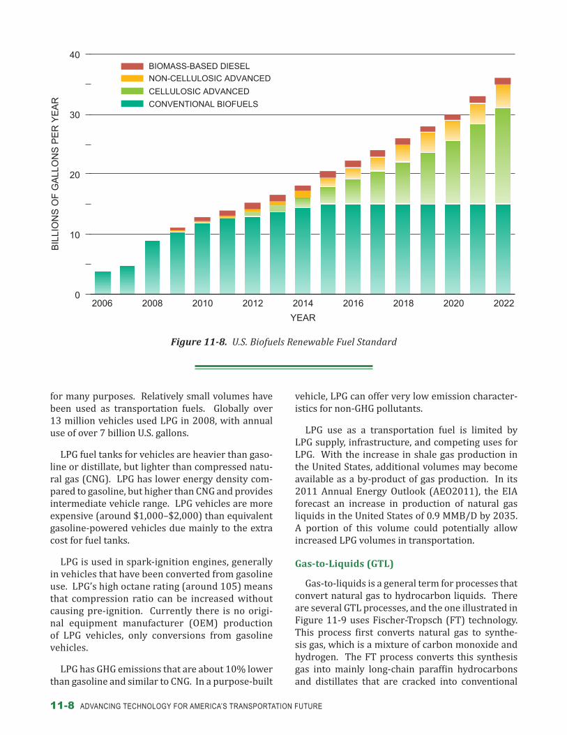
Biofuels are a competing but complementary supply chain to hydrocarbon liquids that intersects at the hydrocarbon product terminal. The ability to incorporate biofuels provides additional sup-ply diversity. Biofuels have been subsidized in the United States for many years and have been recently mandated in two rounds of energy legislation via the renewable fuel standard (RFS) illustrated in Figure 11-8. The biofuel categories under RFS are defined based on GHG performance or feedstock
source. Currently almost all gasoline in the United States contains 10% corn ethanol while biodiesel makes up roughly 2% of U.S. diesel. RFS mandates increasing use of biofuels in the future.
Other Potential Sources of Hydrocarbon Liquids
Liquefied petroleum gas (LPG) and liquids pro-duced from gas and coal provide alternative sources of liquid fuels. Non-LPG pathways are generally more costly and not widely used but offer a future potential for domestic production based on sub-stantial U.S. coal and natural gas reserves.
LpG
LPG is mainly propane with small amounts of other C3 and C4 hydrocarbons. LPG is a by-product of natural gas processing and crude oil refining. LPG is a gas at atmospheric conditions and is stored in liquid form in pressurized tanks at approximately 2–20 bars (30–300 psi) depending on propane/butane composition and storage temperature. LPG is widely available in the United States and is used
YEAR
MIL
LIO
NS
OF
BA
RR
ELS
PE
R D
AY
2012 2010 2008 2006 2004 2002
4
3
2
1
0
-1
-2
Figure 11-7. U.S. Net Imports of Total Petroleum Products(Four-Week Running Average)
Source: U.S. Energy Information Administration.
Figure 11-7. U.S. Net Imports of Total Petroleum Products (Four-Week Running Average)
11-8 ADvANCINg TECHNOLOgY fOR AmERICA’S TRANSPORTATION fUTURE
for many purposes. Relatively small volumes have been used as transportation fuels. Globally over 13 million vehicles used LPG in 2008, with annual use of over 7 billion U.S. gallons.
LPG fuel tanks for vehicles are heavier than gaso-line or distillate, but lighter than compressed natu-ral gas (CNG). LPG has lower energy density com-pared to gasoline, but higher than CNG and provides intermediate vehicle range. LPG vehicles are more expensive (around $1,000–$2,000) than equivalent gasoline-powered vehicles due mainly to the extra cost for fuel tanks.
LPG is used in spark-ignition engines, generally in vehicles that have been converted from gasoline use. LPG’s high octane rating (around 105) means that compression ratio can be increased without causing pre-ignition. Currently there is no origi-nal equipment manufacturer (OEM) production of LPG vehicles, only conversions from gasoline vehicles.
LPG has GHG emissions that are about 10% lower than gasoline and similar to CNG. In a purpose-built
vehicle, LPG can offer very low emission character-istics for non-GHG pollutants.
LPG use as a transportation fuel is limited by LPG supply, infrastructure, and competing uses for LPG. With the increase in shale gas production in the United States, additional volumes may become available as a by-product of gas production. In its 2011 Annual Energy Outlook (AEO2011), the EIA forecast an increase in production of natural gas liquids in the United States of 0.9 MMB/D by 2035. A portion of this volume could potentially allow increased LPG volumes in transportation.
Gas-to-Liquids (GtL)
Gas-to-liquids is a general term for processes that convert natural gas to hydrocarbon liquids. There are several GTL processes, and the one illustrated in Figure 11-9 uses Fischer-Tropsch (FT) technology. This process first converts natural gas to synthe-sis gas, which is a mixture of carbon monoxide and hydrogen. The FT process converts this synthesis gas into mainly long-chain paraffin hydrocarbons and distillates that are cracked into conventional
0
10
20
30
40 B
ILLI
ON
S O
F G
ALL
ON
S P
ER
YE
AR
Figure 11-8. U.S. Biofuels Renewable Fuel Standard
2006 2008 2010 2012 2014 2016 2018 2020 2022
YEAR
CONVENTIONAL BIOFUELS
CELLULOSIC ADVANCED
NON-CELLULOSIC ADVANCED
BIOMASS-BASED DIESEL
Figure 11-8. U.S. Biofuels Renewable Fuel Standard

CHAPTER 11 – HYDROCARBON LIQUIDS 11-9
able for use in a low-level blend. Methanol can also be used as a high-level blend with gasoline, but requires more extensive vehicle upgrading for use in a flexible-fueled-vehicle than ethanol. Since U.S. gasoline fuels currently contain up to 10% ethanol, addition of methanol would result in excessive fuel oxygen content. Therefore methanol would likely displace ethanol in the gasoline blend. DME has high cetane and can substitute for diesel in com-pression ignition engines but would require sig-nificant vehicle and distribution infrastructure addition due to high vapor pressure (similar to LPG) and use of pressurized tanks. Methanol and DME are intermediaries in the MTG process, which results in high octane gasoline and LPG. FT diesel and MTG have an advantage in producing hydro-carbon liquids that can be readily incorporated into the existing infrastructure as finished fuels or blendstocks.
The commercial viability of these technologies is contingent on a number of variables, such as com-peting energy prices (a low gas price relative to oil benefits gas conversion), risk threshold, capital cost and return on capital requirements. Gas conver-sion may hold long-term promise due to the grow-ing extent of the “shale gas” resource in the United States. Potential future production and economic comparisons are discussed later in this chapter.
coal-to-Liquids (ctL)
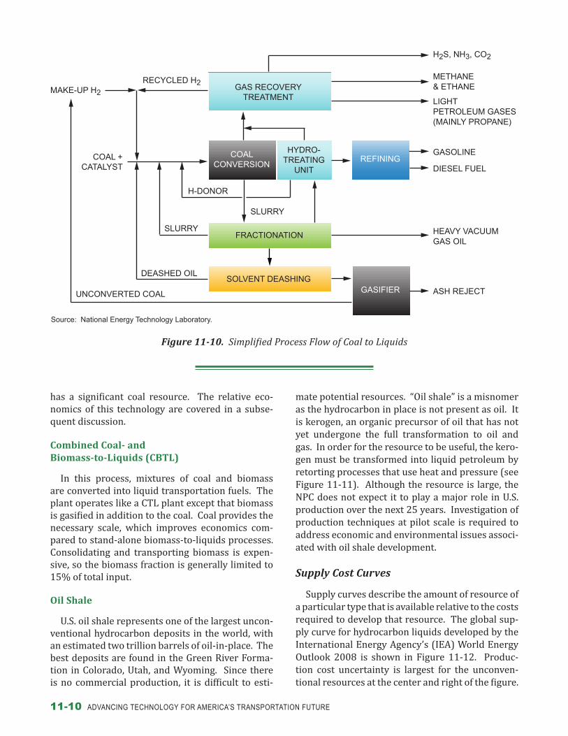
Alternative hydrocarbon liquids can also be derived from coal. There are two main technolo-gies available for coal conversion: indirect and direct liquefaction. Indirect liquefaction is similar to GTL. Coal is transformed into synthesis gas and then converted to liquid hydrocarbon fuels using the processes described above (FT diesel, MTG, methanol, DME). The direct liquefaction process shown in Figure 11-10 involves addition of hydro-gen to coal to increase the hydrogen-to-carbon ratio from ~0.8 in coal to ~1.8 typical of various petro-leum products. The potential for CTL is contingent on a number of factors: coal and petroleum prices, risk threshold, capital cost, and return on capital requirements. Coal is generally the least expensive fossil fuel but capital costs for CTL are higher than GTL due to extra steps needed to convert solid coal to synthesis gas. There are commercial CTL plants in China and South Africa, but no commercial plants in the United States even though the United States
transportation fuels. The process has a high distil-late yield and also produces a lighter fraction that can be used as a gasoline blending component or as a feedstock for chemicals production. The pro-cess energy efficiency in converting natural gas to liquid products is 58–65%.4 There are GTL plants operating in Malaysia, South Africa, and Qatar, with additional plants under construction in Qatar and Nigeria.
Natural gas can also be converted to other trans-portation fuels such as methanol, dimethyl ether (DME), or methanol-to-gasoline (MTG). Both methanol and DME require significant fueling and vehicle infrastructure investments, which makes them less attractive than other liquid fuels pro-duced from natural gas. Commercial production of methanol is well established. Methanol can be used in vehicles as a low-level blend with gasoline. It has higher vapor pressure than gasoline and is less water tolerant, which may make it less suit-
4 Carmine L. Iandoli and Signe Kjelstrup, “Exergy Analysis of a GTL Process Based on Low-Temperature Slurry F-T Reactor Technology with a Cobalt Catalyst,” Energy Fuels 21, no. 4 (2007): pages 2317-2324.
Figure 11-9. Simplified Process Flow of Gas-to-Liquids
AIR NATURAL GAS
AIRSEPARATION
OXYGEN
GASPROCESSING
METHANE
GASLIQUIDS
GAS SYNTHESIS
CARBON MONOXIDEAND HYDROGEN
FISCHER-TROPSCHPROCESS
CRACKING
LIQUIDHYDROCARBONS
DIESEL NAPHTHA PARAFFIN
Figure 11-9. Simplified Process Flow of Gas-to-Liquids
11-10 ADvANCINg TECHNOLOgY fOR AmERICA’S TRANSPORTATION fUTURE
mate potential resources. “Oil shale” is a misnomer as the hydrocarbon in place is not present as oil. It is kerogen, an organic precursor of oil that has not yet undergone the full transformation to oil and gas. In order for the resource to be useful, the kero-gen must be transformed into liquid petroleum by retorting processes that use heat and pressure (see Figure 11-11). Although the resource is large, the NPC does not expect it to play a major role in U.S. production over the next 25 years. Investigation of production techniques at pilot scale is required to address economic and environmental issues associ-ated with oil shale development.
Supply Cost Curves
Supply curves describe the amount of resource of a particular type that is available relative to the costs required to develop that resource. The global sup-ply curve for hydrocarbon liquids developed by the International Energy Agency’s (IEA) World Energy Outlook 2008 is shown in Figure 11-12. Produc-tion cost uncertainty is largest for the unconven-tional resources at the center and right of the figure.
has a significant coal resource. The relative eco-nomics of this technology are covered in a subse-quent discussion.
combined coal- and biomass-to-Liquids (cbtL)
In this process, mixtures of coal and biomass are converted into liquid transportation fuels. The plant operates like a CTL plant except that biomass is gasified in addition to the coal. Coal provides the necessary scale, which improves economics com-pared to stand-alone biomass-to-liquids processes. Consolidating and transporting biomass is expen-sive, so the biomass fraction is generally limited to 15% of total input.
oil Shale
U.S. oil shale represents one of the largest uncon-ventional hydrocarbon deposits in the world, with an estimated two trillion barrels of oil-in-place. The best deposits are found in the Green River Forma-tion in Colorado, Utah, and Wyoming. Since there is no commercial production, it is difficult to esti-
Figure 11-10. Simplified Process Flow of Coal-to-Liquids
REFININGGASOLINE
DIESEL FUEL
H-DONOR
SLURRYFRACTIONATION HEAVY VACUUM
GAS OIL
DEASHED OILSOLVENT DEASHING
UNCONVERTED COAL GASIFIER ASH REJECT
MAKE-UP H2
RECYCLED H2GAS RECOVERY
TREATMENT
H2S, NH3, CO2
METHANE& ETHANE
LIGHT PETROLEUM GASES (MAINLY PROPANE)
COAL +CATALYST
COALCONVERSION
HYDRO-TREATING
UNIT
SLURRY
Source: National Energy Technology Laboratory.
Figure 11-10. Simplified Process Flow of Coal to Liquids

CHAPTER 11 – HYDROCARBON LIQUIDS 11-11
Figure 11-11. Simplified Process Flow of Oil Shale
OIL SHALE DEPOSIT
FRACTURING
RETORTING
PRODUCT RECOVERY
MINING
CRUSHING
RETORTING
SPENT SHALE
REFINING
LIQUID FUELS BY-PRODUCTS
Figure 11-12. Long-Term Oil Supply Cost Curve
Note: The figure shows the availability of oil resources as a function of the estimated production cost. Cost associated with CO2 emissions is not included. There is also a significant uncertainty on oil shales production cost as the technology is not yet commercial. The shading and overlapping of the gas-to-liquids and coal-to-liquids segments indicates the range of uncertainty surrounding the size of these resources, with 2.4 trillion shown as a best estimate of the likely total potential for the two combined.
Source: International Energy Agency, World Energy Outlook 2008, © OECD/IEA 2008.
0
20
40
60
80
100
120
0 1,000 2,000 3,000 4,000 5,000 6,000 7,000 8,000 9,000
ARCTIC
EOR
MIDDLE EASTAND NORTH
AFRICA
RESOURCES (BILLION BARRELS)
PR
OD
UC
TIO
N C
OS
T (
2008
DO
LLA
RS
)
GAS-TO-LIQUIDS
COAL-TO-LIQUIDS
OTHERCONVENTIONAL
OIL
PRODUCED
HEAVYOIL ANDBITUMEN
CO2–EOR OILSHALES
DEEPWATER ANDULTRA-DEEPWATER
Figure 11-11. Simplified Process Flow of Oil Shale
Figure 11-12. Long-Term Oil-Supply Cost Curve

11-12 ADvANCINg TECHNOLOgY fOR AmERICA’S TRANSPORTATION fUTURE
The amount of hydrocarbon resources that can be brought to market may be as high as 9 trillion bar-rels, compared to roughly 1 trillion barrels that have already been produced. The lowest cost conven-tional production is in the Middle East and North Africa. Oil shales, GTL, and CTL represent the most costly supply.
The hydrocarbon liquid supply curve provides a benchmark for competing fuel technologies. Costs of oil shale and XTL (gas-, coal-, and biomass-to-liquids) may be competitive with potential fuel pathway alternatives in the center of the sup-ply curve. The abundance of hydrocarbon liquid resources combined with the existing infrastruc-ture of refining, pipelines, and dispensing makes hydrocarbon liquids a formidable incumbent in the future of transportation fuels.
FuturE pEtroLEum SuppLy and dEmand
Supply and demand outlooks are published annually by the EIA and the IEA. Additionally, the National Petroleum Council conducted a study of North American resources, titled Prudent Develop-ment: Realizing the Potential for North America’s Abundant Natural Gas and Oil Resources, which was published in 2011. The NPC study included fore-casts from EIA and IEA as well as a wide range of industry organizations and consultants to develop low, medium, and high scenarios for North Ameri-can oil production.
There is considerable uncertainty in projecting future behavior of energy markets, which increases with the length of the outlook. Outlooks are based on a set of assumptions regarding economic growth, oil prices, government action, and other factors. The reader is referred to the NPC Prudent Develop-ment report for more full discussion on petroleum supply and demand.
price assumptions AEO2010 oil price cases, shown in Figures
11-13 through 11-16, represent alternative, inter-nally consistent scenarios. In general, EIA and IEA price scenarios are similar. Demand, production, and imports of liquid fuels are all sensitive to the assumed long-term path of oil prices. Demand is reduced in the high price scenario while domestic
2005 2010 2020 2025 2030
HIGH OIL PRICE
LOW OIL PRICE
REFERENCE
PROJECTIONS
MIL
LIO
NS
OF
BA
RR
ELS
PE
R D
AY
YEAR2015
Figure 11-14. Liquids Outlook overPrice Scenarios in AEO2010 –
U.S. Liquids Consumption
ALSO USED AS FIG. 8-7
20350
5
10
15
20
25
30
Source: U.S. Energy Information Administration, Annual Energy Outlook 2010.
0
50
100
150
200
250
1980 1990 2010 2020 2030
Figure 11-13. Liquids Outlook over Price Scenarios in AEO2010 – Average Annual World Oil Prices
ALSO USED AS FIG. 8-6
LOW OIL PRICE
HIGH OIL PRICE
REFERENCE
PROJECTIONS
2008
DO
LLA
RS
PE
R B
AR
RE
L
YEAR2000
Source: U.S. Energy Information Administration, Annual Energy Outlook 2010.
Figure 11-14. Liquids Outlook over Price Scenar-ios in AEO2010 – U.S. Liquids Consumption
Figure 11-13. Liquids Outlook over Price Scenar-ios in AEO2010 – Average Annual World Oil Prices

CHAPTER 11 – HYDROCARBON LIQUIDS 11-13
production increases, thereby lowering crude imports. U.S. supply is more sensitive to assumed prices than demand.
Global Supply and demand
According to the IEA, future demand growth for hydrocarbon liquids is focused in the developing world, where large increases in end-user demand overwhelm efficiency gains (see Figure 11-17). China alone accounts for almost half of the projected growth in transportation-related oil demand over the next 25 years. In contrast, use of oil in mature OECD countries is forecast to decrease as increasing efficiency outweighs relatively slow growth in end-user demand. Meeting the increase in non-OECD oil demand is a major challenge for the global hydro-carbon liquid supply chain.
More recent EIA and IEA outlooks have tended to forecast lower global oil production in future years. This reflects difficulty in increasing conven-tional production combined with reduced demand projections due to higher prices, slower economic growth, and increased regulation of vehicle fuel economy. Unconventional liquids play a grow-ing role in all global outlooks. Figure 11-18 from the AEO2010 outlook illustrates the potential of unconventional liquid supply.
north american oil Supply
Oil production forecasts for the United States and North America have become more positive in recent years. There has been a steady upward revision in projected future U.S. oil production as new unconventional oil plays continue to develop. Long-term growth in oil production can come from several existing and new North American sup-ply sources including tight oil, offshore oil, Arctic oil, oil sands and oil shale. The AEO2011 calls for U.S. and North American production to increase through 2035. This is consistent with the NPC Prudent Development study, which also indicates that North American production could potentially double by 2035 in a high-side scenario as shown in Figure 11-19. Large increases in Canadian oil pro-duction are expected due to increases in oil sands production.
The NPC Prudent Development study also cate-gorized U.S. shale gas as a potential game changer.
Figure 11-16. Liquids Outlook over Price Scenarios in AEO2010 – U.S. Liquid Imports
ALSO USED AS FIG. 8-9
0
10
20
30
40
50
1990 2010 2020 2030
LOWOIL PRICE
HIGH OIL PRICE
REFERENCE
PROJECTIONS
PE
RC
EN
T
YEAR
2000
60
70
Source: U.S. Energy Information Administration, Annual Energy Outlook 2010.
2005 2010 2020 2025 2030
LOW OIL PRICE
HIGHOIL PRICE
REFERENCE
PROJECTIONSM
ILLI
ON
S O
F B
AR
RE
LS P
ER
DA
Y
YEAR
2015 20350
4
8
12
16
Figure 11-15. Liquids Outlook over Price Scenarios in AEO2010 –U.S. Liquids Production
ALSO USED AS FIG. 8-8
Source: U.S. Energy Information Administration, Annual Energy Outlook 2010.
Figure 11-16. Liquids Outlook over Price Scenarios in AEO2010 – U.S. Liquids Imports
Figure 11-15. Liquids Outlook over Price Scenar-ios in AEO2010 – U.S. Liquids Production

11-14 ADvANCINg TECHNOLOgY fOR AmERICA’S TRANSPORTATION fUTURE
Figure 11-17. Change in Oil Demand from 2010 to 2035 by Sector and Region
– 5
0
5
10
15
20
OTHER*BUILDINGS ANDAGRICULTURE
INDUSTRYTRANSPORT
MIL
LIO
NS
OF
BA
RR
ELS
PE
R D
AY
* Includes power generation, other energy sector, and non-energy use.Source: International Energy Agency, World Energy Outlook 2010, © OECD/IEA 2010.
INTER-REGIONAL (BUNKERS)
OTHER NON-OECD
CHINA
OECD
Figure 11-18. Unconventional Hydrocarbon Liquids in AEO2010 Oil Price Cases
Also used as Fig. 8-10
0
5
10
15
20
25
2008 LOW OIL PRICE REFERENCE 2035
HIGH OIL PRICE
PE
RC
EN
T
SHALE
GTL
CTL
BIOFUEL
EXTRA HEAVY OIL
BITUMEN
Source: U.S. Energy Information Administration, Annual Energy Outlook 2010.
Figure 11-17. Change in Oil Demand from 2010 to 2035 by Sector and Region
Figure 11-18. Unconventional Hydrocarbon Liquids in AEO2010 Oil Price Cases

CHAPTER 11 – HYDROCARBON LIQUIDS 11-15
light-duty demand and further reduce petroleum imports.
transportation demand
Additional detail in transportation fuel demand is shown in Figure 11-21. The EIA projects decreasing gasoline demand to 2035 while diesel and jet fuel are forecast to increase slightly. The role of biofuels also increases.
rEFininGRefining Technology
U.S. refineries are some of the most highly com-plex in the world, producing high-quality transpor-tation fuels and undergoing continual upgrades to
Increased natural gas production is also expected to result in increased production of natural gas liquids. LPG, butane, and natural gasoline are all potential transportation fuels either as blend-stocks or in specialized vehicles.
Supply and demand balance and imports
As shown in Figure 11-20, the EIA forecasts that U.S. liquid fuel use remains near its present level through 2035 (AEO2012 Early Release). Oil imports are projected to decrease due to increases in U.S. petroleum and biofuel supply, which outpaces the small increase in demand. The EIA outlook does not include proposed light-duty vehicle CAFE (corporate average fuel econ-omy) and GHG standards, which would reduce
0
10
20
2010LIMITED HIGH POTENTIAL
MIL
LIO
NS
OF
BA
RR
ELS
PE
R D
AY
Figure 11-19. U.S. and Canadian Oil Production Projections
Notes: The oil supply bars for 2035 represent the range of potential supply from each of the individual supply sources and types considered in this study. The specific factors that may constrain or enable development and production can be different for each supply type, but include such factors as whether access is enabled, infrastructure is developed, appropriate technology research and development is sustained, an appropriate regulatory framework is in place, and environmental performance is maintained.
In 2010, oil demand for the U.S. and Canada combined was 22.45 million barrels per day. Thus, even in the high potential
scenario, 2035 supply is lower than 2010 demand, implying a continued need for oil imports and participation in global trade.
Source: Historical data from Energy Information Administration and National Energy Board of Canada. Projections from National Petroleum Council, Prudent Development: Realizing the Potential of North America’s Abundant Natural Gas and Oil Resources, 2011.
5
15
25
2035
UNCONVENTIONAL OIL:
OIL SHALE
TIGHT OIL
OIL SANDS
ARCTIC
NATURAL GAS LIQUIDS
OFFSHORE
ONSHORE CONVENTIONAL
Art Area is 42p x 31p
Figure 11-19. U.S. and Canadian Oil Production Projections

11-16 ADvANCINg TECHNOLOgY fOR AmERICA’S TRANSPORTATION fUTURE
0
5
10
15
20
25
1970 1980 1990 2000 2010 2020 2030 2040
MIL
LIO
NS
OF
BA
RR
ELS
PE
R D
AY
YEAR
U.S. SUPPLY
U.S. CONSUMPTION
Figure 11-20. Liquid Supply and Demand Balance in AEO2012 Early Release
IMPORTS
Source: U.S. Energy Information Administration, Annual Energy Outlook 2012 Early Release.
Figure 11-21. Transportation Fuel Projection in AEO2012 Early Release
ALSO USED AS FIG. 8-12
0
4
8
12
16
2010 2015 2020 2025 2030 2035
MIL
LIO
NS
OF
BA
RR
ELS
PE
R D
AY
YEAR
BIOFUELS JET FUEL DIESEL GASOLINE
Source: U.S. Energy Information Administration, Annual Energy Outlook 2012 Early Release.
Figure 11-20. Liquid Supply and Demand Balance in AEO2012 Early Release
Figure 11-21. Transportation Fuel Projection in AEO 2012 Early Release

CHAPTER 11 – HYDROCARBON LIQUIDS 11-17
5. Auxiliary Operating Facilities. These units support operation of the primary processing units by providing inputs like hydrogen or processing by-products.
6. Refinery Off-Site Facilities. These facilities provide utilities, logistics, and safety.
Table 11-1 shows the six categories of refin-ery processes. A detailed discussion is in Appendix C, “History and Fundamentals of Refin-ing Operations,” of the June 2000 NPC report U.S. Petroleum Refining.
Refinery Schematic. Refinery units are care-fully integrated to provide high product yield with minimum waste and energy consumption. While each refinery is unique, refineries can be classi-fied into three broad groups based on process-ing complexity, which in turn determines ability to convert crude oil into lighter transportation fuels. Hydro-skimming refineries contain a crude oil distillation unit (CDU) and naphtha reform-ers, which increase gasoline octane and produce hydrogen that can be used in desulfurization units. Medium conversion, or cracking, refiner-ies have the same elements plus fluid catalytic cracking (FCC) and alkylation units, which allows greater conversion of crude oil to transportation fuels. High conversion refineries also have cokers, hydrocrackers, and hydrogen plants, as shown in Figure 11-22. High conversion refineries are common in the United States and convert large proportions of crude oil feedstock to transpor-tation fuels and have greater ability to upgrade heavy or sour crude oil. Integration and optimi-zation becomes more important as the number of process streams increase. Modern refineries contain networks of sensors, logic devices, and computers to control and optimize the complex reactions and flows within and among process and for logistics and planning of crude oil inputs and product output.
industry State
Geographic Distribution. Refining capacity is generally based on CDU capacity with units of thousand barrels per day. The majority of U.S. refineries are geographically concentrated into several large refining centers, called Petroleum
improve efficiency, product quality, and feedstock utilization.
Background. Liquid hydrocarbon fuels must have known and consistent properties for specific types of combustion systems. Manufacturing prod-ucts at very large scale and at the molecular level makes refining unique and requires a wide range of technologies.
In addition to transportation fuels, the refining sector provides a number of products that play an essential role in the economy.5
y Petrochemicals. The refining sector is closely integrated with petrochemicals. The exchange of feedstocks and products between refineries and petrochemicals plants improves competitiveness in industrial clusters such as the U.S. Gulf Coast.
y Industrial Materials. The refining industry also plays a role in other industrial value chains: asphalt for road construction and roofing, lubri-cants for use in transportation and industry, high-quality petroleum coke for use in the met-als industry, waxes, solvents, and other products. Many of these specialty products are difficult to manufacture and highly specialized.
Refining Processes. Refinery processes can be divided into six categories:
1. Separation of Crude Oil. Separates crude into materials with narrower boiling range.
2. Restructuring Hydrocarbon Molecules. Restructuring processes change molecular size or structure in a variety of ways. Some processes break apart bigger molecules while others combine small gas molecules to make liquids, and others change molecular structure. Examples are listed in Table 11-1.
3. Treating. Treating processes are used to remove contaminants such as sulfur, nitrogen, and heavy metals, which are present in crude oil, from various streams.
4. blending Hydrocarbon Products. Many streams are blended to make gasoline and other hydrocarbon products.
5 Europia, White Paper on EU Refining, 2011.

11-18 ADvANCINg TECHNOLOgY fOR AmERICA’S TRANSPORTATION fUTURE
SeparationMolecule
RestructuringTreating Product Blending Auxiliaries Off-Sites
Desalting & Dewatering
Atmospheric Distillation
Vacuum Distillation
Conversion
y Thermal Cracking
− Steam Cracking − Visbreaking − Coking
y Catalytic Cracking
− Fluid Catalytic Cracking
Hydrocracking
Combining
y Alkylation
y Polymerization
Modifying
y Catalytic Reforming
y Isomerization
y Ethers Manu-facture
Hydroprocessing
Amine Treating
Sweetening
Solvent Extraction
Bitumen Production
Wax, Lube, and Grease Manufacturing
Motor Gasoline
y Reformate
y Alkylate
y Straight-Run Gasoline
y FCC Gasoline
y Coker Gasoline
y Butane
y Oxygenates
y Additives
Jet Fuel
y Kerosene
y Straight-Run Virgin Distillates
y Naphtha
Diesel Fuel
y Virgin Distillates
y Cycle Oil
Distillate Fuel Oil
Residual Fuels
Lubes
y Refined Base Stock
y Additives
Asphalt
y Residual Base Stock
y Additives
Liquefied Petroleum Gas (LPG)
Petrochemical Feedstocks
y Benzene
y Toluene
y Ethane
y Ethylene
y Propane
y Propylene
y Naphtha
y Gas Oils
Petroleum Solvents
Hydrogen Production
Light Ends Recovery
Acid Gas Treating
Sour Water Stripping
Sulfur Recovery
Tail Gas Treating
Wastewater Treatment
Storage Tanks
Steam Generation
Power Generation
Flare & Blowdown Systems
Cooling Water Systems
Receiving & Distribution Systems
Refinery Fire Control Systems
Garages
Maintenance Shops
Storehouses
Laboratories
Necessary Office Buildings
Source: Appendix C, “History and Fundamentals of Refining Operations,” in NPC report U.S. Petroleum Refining, June 2000.
Table 11-1. Six Categories of Refinery Processes

CHAPTER 11 – HYDROCARBON LIQUIDS 11-19
RE
FO
RM
ER
HY
DR
OG
EN
ME
DIU
M G
AS
OIL
PR
OP
AN
E/B
UT
AN
E
HE
AV
Y F
UE
L O
IL
HY
DR
OG
EN
PLA
NT
CO
KE
GA
S
CR
UD
EO
ILU
NIT
VA
CU
UM
UN
IT
LIG
HT
GA
S O
IL
DIS
TIL
LAT
ION
TO
WE
R
HIG
H-S
ULF
UR
KE
RO
SE
NE
/JE
T F
UE
L LO
W-S
ULF
UR
KE
RO
SE
NE
/JE
T F
UE
L
LOW
-SU
LFU
R D
IES
EL/
HE
AT
ING
OIL
HIG
H-O
CT
AN
E G
AS
OLI
NE
Fig
ure
11-2
2. S
impl
ified
Pro
cess
Flo
w D
iagr
am fo
r H
igh
Con
vers
ion
(Cok
ing/
Res
id D
estr
uctio
n) R
efin
ery
ME
DIU
M/
HE
AV
YS
OU
R
CR
UD
E
Sou
rce:
Val
ero
(web
site
), In
dust
ry F
unda
men
tals
, “B
asic
s of
Ref
inin
g an
d C
okin
g,”
Janu
ary
2011
, http
://w
ww
.val
ero.
com
/Inve
stor
Rel
atio
ns/P
ages
/Indu
stry
Fun
dam
enta
ls.a
spx.
LOW
-OC
TA
NE
GA
SO
LIN
E A
ND
NA
PH
TH
A
HIG
H-S
ULF
UR
DIE
SE
L/H
EA
TIN
G O
IL
ULT
RA
LOW
-SU
LFU
R J
ET
/DIE
SE
L
PR
OP
AN
E/B
UT
AN
E
ALK
Y G
AS
OLI
NE
ALK
YLA
TIO
NU
NIT
FC
C G
AS
OLI
NE
Art
Are
a is
57p
x 4
0p
HY
DR
OC
RA
CK
AT
E G
AS
OLI
NE
HY
DR
OC
RA
CK
ER
DE
LAY
ED
CO
KE
R
DIS
TIL
LAT
ED
ES
ULF
UR
IZE
R
=
FLU
IDC
AT
ALY
TIC
CR
AC
KE
R
ELE
ME
NT
S C
ON
TAIN
ED
ON
LY IN
H
IGH
CO
NV
ER
SIO
N R
EF
INE
RIE
S
Figu
re 1
1-22
. Si
mpl
ified
Pro
cess
Flo
w D
iagr
am fo
r Hig
h Co
nver
sion
(Cok
ing/
Resi
d De
stru
ctio
n) R
efin
ery
11-20 ADvANCINg TECHNOLOgY fOR AmERICA’S TRANSPORTATION fUTURE
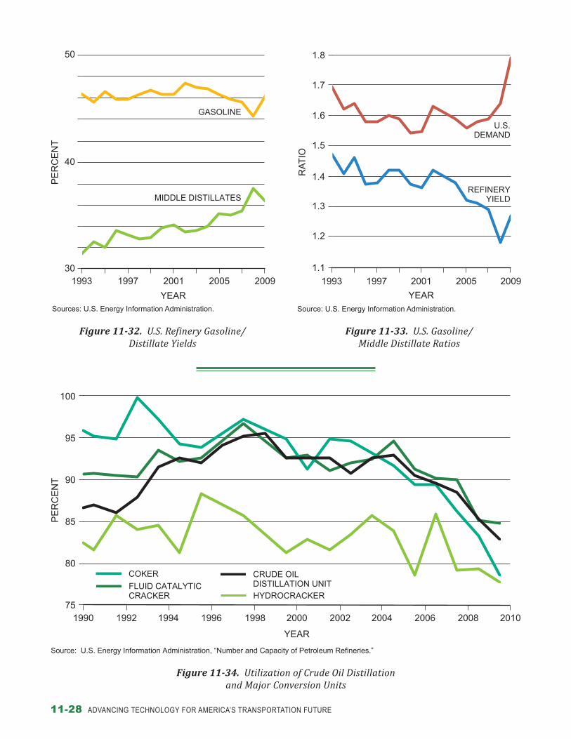
Complexity. As additional conversion units are added to a refinery, ability to convert heavier feed-stock into transportation fuels increases. As shown in Figure 11-24, U.S. conversion capability has increased over the last 20 years. U.S. coker capacity has grown by 68%, hydrocracker capacity by 44%, FCC capacity by 13%, and hydrotreating capacity by 68% over the period.
Product Quality Improvement. The qualities of hydrocarbon produced by refiners have improved over time to meet regulatory standards and the evolution of the transportation fleet. Increasingly, hydrocarbon fuel product specifications are driven
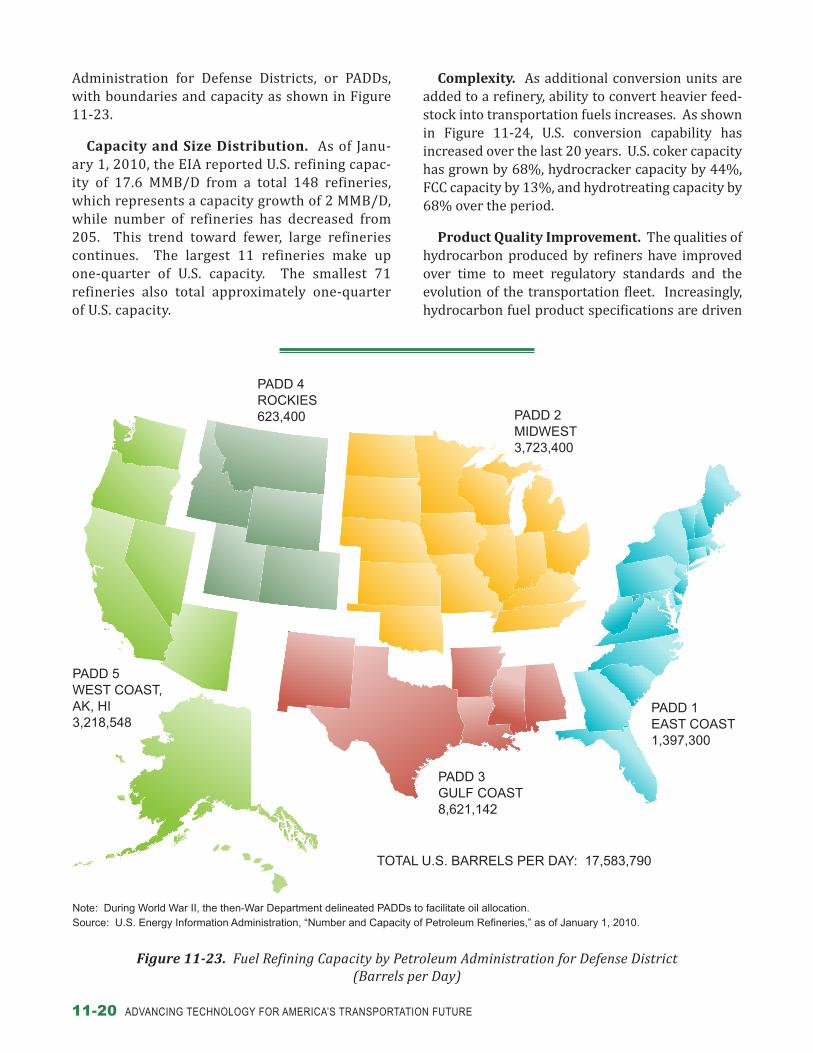
Administration for Defense Districts, or PADDs, with boundaries and capacity as shown in Figure 11-23.
Capacity and Size Distribution. As of Janu-ary 1, 2010, the EIA reported U.S. refining capac-ity of 17.6 MMB/D from a total 148 refineries, which represents a capacity growth of 2 MMB/D, while number of refineries has decreased from 205. This trend toward fewer, large refineries continues. The largest 11 refineries make up one-quarter of U.S. capacity. The smallest 71 refineries also total approximately one-quarter of U.S. capacity.
Figure 11-23. Fuel Refining Capacity by Petroleum Administration for Defense Districts (Barrels per Day)
PADD 1 EAST COAST1,397,300
PADD 3GULF COAST8,621,142
PADD 2 MIDWEST3,723,400
PADD 4ROCKIES623,400
PADD 5WEST COAST, AK, HI3,218,548
Note: During World War II, the then-War Department delineated PADDs to facilitate oil allocation.Source: U.S. Energy Information Administration, “Number and Capacity of Petroleum Refineries,” as of January 1, 2010.
TOTAL U.S. BARRELS PER DAY: 17,583,790
Art Area is 42p x 35p6
Figure 11-23. Fuel Refining Capacity by Petroleum Administration for Defense District (Barrels per Day)

CHAPTER 11 – HYDROCARBON LIQUIDS 11-21
by vehicle technical requirements and environmen-tal regulations that have significantly reduced vehi-cle emissions over the past 40 years. The ability of refiners to adapt to the regulations has been well established; however, sometimes significant capital funds are required.
Efficiency Improvements by Refiners. Refin-ers have reduced energy consumption through efficiency improvements, energy integration, and efficiency investments. Improvement comes from numerous small items as well as larger projects like cogeneration and advanced catalyst technology. Today refining is highly efficient, with roughly 90% of energy in crude oil remaining in finished prod-ucts.6 Since 1986, the refining sector has improved its energy efficiency by roughly 0.6% per year (see Figure 11-25). Efficiency gains slowed after 1998 as cleaner fuel standards were adopted, which required additional processing for sulfur reduction and other specification changes.
6 GREET Model: The Greenhouse Gases, Regulated Emissions, and Energy Use in Transportation Model, Argonne National Laboratory, http://greet.es.anl.gov/.
0
10
20
30
40
50
60
70
80
90
100
1990 1992 1994 1996 1998 2000 2002 2004 2006 2008 2010
Source: U.S. Energy Information Administration, “Number and Capacity of Petroleum Refineries.”
Figure 11-24. Conversion Process Capacity as Percent of Crude Oil Distillation Unit
PE
RC
EN
T
YEAR
HYDROTREATERFLUID CATALYTIC CRACKERCOKERHYDROCRACKER
84
88
92
96
100
1986 1990 1994 1998 2002 2006
RFG1 RFG2 TIER 2 ULSDLSD
Figure 11-25. U.S. RefineryEnergy Intensity Index
Note: Fuel Regulations: LSD = Low-Sulfur Diesel; RFG = Reformulated Gasoline; TIER 2 = Low-Sulfur Gasoline; ULSD = Ultra-Low-Sulfur DieselSource: Solomon Associates.
PE
RC
EN
T O
F 1
986
LEV
ELS
YEAR
DECREASINGENERGY
USE
Figure 11-24. Conversion Process Capacity as Percent of Crude Oil Distillation Unit
Figure 11-25. U.S. Refinery Energy Intensity Index

11-22 ADvANCINg TECHNOLOgY fOR AmERICA’S TRANSPORTATION fUTURE
by water movements. The final part of the journey is via truck from terminals to fuel marketers and retail locations. This system, with the exception of pipelines, has been adapted to handle ethanol and biodiesel. Ethanol also takes advantage of rail movements where feasible.
Throughout the early decades of the petroleum industry, refined products were manufactured at rel-atively small refineries located close to product mar-kets. During World War II, vulnerability of tanker shipments and the growing demand for petroleum products led to the development of large pipelines to move products to the East Coast from refining cen-ters along the Gulf Coast. Shortly thereafter, pipe-lines were constructed in the Midwest and West. Approximately 75% of the existing pipeline infra-structure was constructed between 1940 and 1980.
The distribution of hydrocarbon liquid product terminals has grown to span the entire country, as
Refinery Capability to Adapt to Shifting Feed-stock Mix/Quality. Crude oil varies in a number of properties including sulfur, density, acidity, and others. Refineries have limited ability to change crude oil inputs and are often designed and opti-mized to run nearby or readily available crudes. Changing crude oil feedstock properties usually requires capital investment. A recent example is upgrades to certain Midwest refineries to process Canadian crude from oil sands.
diStribution inFraStructurE
The U.S. refined product distribution system has historically adapted to provide the most efficient and lowest cost product transportation to the U.S. consumer and it will continue to adapt in the fore-seeable future. The distribution system has a back-bone of large, high volume pipelines, supplemented
Figure 11-26. Major U.S. Product Terminals
Source: IRS Active Fuel Terminals.
Figure 11-26. Major U.S. Product Terminals

CHAPTER 11 – HYDROCARBON LIQUIDS 11-23
into a succeeding lower quality material (such as premium gasoline into regular gasoline). Down-grading from one batch to another cannot always occur. In those situations it becomes necessary to segregate the interface (called transmix) and arrange for it to be sent back to the refinery or other processing facility.
Today, pipelines are controlled by the use of com-puters often referred to as programmable logic controllers (PLCs). The data from the PLCs are transferred by secured wide-area network to a cen-tralized database. The data are then compiled and formatted in such a way that a control room opera-tor can make decisions to start or stop the pipeline, adjust flow rates, raise or reduce the operating pressure, as well as open and close valves. The sys-tem of computers and the communications network is collectively referred to as a Supervisory Control
shown in Figures 11-26 and 11-27. These terminals are located in demand centers and along pipeline routes to deliver hydrocarbon fuels and biofuels to the end customer. The legacy value of these termi-nals is significant, for a competing energy pathway to replicate this coverage and redundancy is a very large hurdle.
Over time, the transportation of petroleum prod-ucts has become more complex. For pipeline opera-tors, the proliferation of product grades for gasoline and diesel are a complicating factor that required expanding the number of segregations. These seg-regations create additional complexity in managing product quality and integrity (Figure 11-28).
Depending upon the specifications of adjacent batches, it may be possible to downgrade the com-mingled product interface between two batches
Figure 11-27. Major U.S. Pipelines

11-24 ADvANCINg TECHNOLOgY fOR AmERICA’S TRANSPORTATION fUTURE
ond highest level of ton-miles in 2008, 16% of crude oil, and 27% of petroleum products.
Ethanol impact on infrastructureThe volumes and the percentage of products
transported within the Association of Oil Pipe Lines (AOPL) data do not include ethanol. Pipe-line operators have been reluctant to ship ethanol, or gasoline-ethanol blends on a commercial scale due to ethanol’s corrosive properties and water solubility. Ethanol will clean the internal surfaces of a pipeline and can result in the pipeline becom-ing more susceptible to internal stress corrosion cracking, which is difficult to detect and manage. Likewise, ethanol has an affinity for moisture and is completely soluble in water. Water enters the pipeline system through terminal and refinery tank roofs and can be dissolved in fuels during the refining process. If the ethanol or gasoline-ethanol blend picks up water in the pipeline, it could “phase separate” resulting in off-specification product. An E10 gasoline-ethanol blend can typically contain up to 0.5 volume percent water at 60°F before phase separation occurs. Lesser amounts of water
and Data Acquisition (SCADA) system. The SCADA system can also feed various real time data into business computers to support pipeline scheduling, product accounting, and other business functions (Figure 11-29).
Although pipelines are the primary source for transporting crude oil and refined petroleum prod-ucts, water carriers, railroads, and trucks are also important components. However, the ability to continuously move large volumes of crude oil and refined products over great distances have made pipelines the most efficient mode of transporta-tion. Likewise, the economics when transporting products by pipeline are also favorable. The rela-tive shares of refined product movements by mode are shown in Figure 11-30.
oil pipelines – State of the industryPipelines accounted for 71% of all petroleum
transportation in 2008, up from approximately 54% in 1990.7 Water carriers provided the sec-
7 Association of Oil Pipe Lines, Report on Shifts in Petroleum Transportation: 1990–2009, February 2012.
Figure 11-28. Typical Refined Products Pipeline Batch Sequencing
Figure 11-28. Typical Refined Products Pipeline Batch Sequencing
DIRECTION OF FLOW
REFORMULATEDREGULARGASOLINE
ULTRA LOWSULFURDIESEL
KEROSENE /JET FUEL
CONVENTIONALREGULARGASOLINE
CONVENTIONALPREMIUMGASOLINE
REFORMULATEDPREMIUMGASOLINE
REFORMULATEDREGULARGASOLINE
STORAGE
BATCH 1 BATCH 7BATCH 6BATCH 5BATCH 4BATCH 3BATCH 2

CHAPTER 11 – HYDROCARBON LIQUIDS 11-25
Figure 11-29. SCADA System
Figure 11-30. Total Petroleum Product Movement
E-1
PLC-1 PLC-2
L
SCADA
FM
FLOW
V-2
LEVEL
Source: Kinder Morgan.
Figure 11-29. SCADA System
SCADA system reads the measurementflow and level, and sends the set point tothe programmable logic controller (PLC).
PLC-1 compares the measured flow to the set point, controls the pump speed as required to match the flow to set point.
PLC-2 compares the measured level to the level set point, controls the flow through the valve to match the level to set point.
PUMPCONTROL
VALVECONTROL
DATASTORAGE
0
100
200
300
400
500
600
1990 1995 2000 2005
BIL
LIO
NS
OF
TO
N-M
ILE
S
Figure 11-30. Total Petroleum Products Ton-Miles
YEARSource: Association of Oil Pipe Lines.
RAILROADS
MOTOR CARRIERS
WATER CARRIERS
PIPELINES

11-26 ADvANCINg TECHNOLOgY fOR AmERICA’S TRANSPORTATION fUTURE
there are several important issues as discussed below.
conventional infrastructureResources
As discussed previously, conventional oil is increasingly located in remote areas or geographi-cally concentrated in a few countries with large remaining resources. Access to these resources, technology development, and safe and environ-mentally sound operations are critical to meeting projected increases in demand. Unconventional resources are also important, with technology devel-opment to reduce cost and improve environmental performance an important challenge. Issues associ-ated with resource development are covered in the NPC Prudent Development report.
Impact of Outlooks on Product Demand and Refining
The crude oil production profiles shown in Fig-ure 11-19 foresee an increase in North American unconventional oil production. The crude oil slate shift will provide an incentive for upgrading of heavy crude oil in existing infrastructure. The most efficient disposition of this heavy crude oil produc-tion will likely be in existing high conversion refin-eries discussed previously in this chapter.
As the crude oil profiles change, so will the demand barrel as illustrated in the Reference and Alternative scenarios shown in Figure 11-31. The AEO2012 Early Release and the IEA outlooks show the potential pressure on refined gasoline from a volume and yield perspective due to light-duty fleet efficiency, increased biofuels, and growth in diesel for medium-/heavy-duty vehicles. The challenge for refining will be to make the product slates required by customer demands. Although the changes are substantial in some outlooks, they occur over a very long period, giving industry time to respond. The flexibility of the refinery fleet to manage this shift will be discussed in the next section.
Refinery Capability to Address Shape of Barrel Shifts
The U.S. refining industry has responded in the past to changing customer demand by shifting refin-ery yields. Recently, U.S. refineries have increased distillate yield, from 31.9% in 1995 to 36.3% in
can induce separation at lower temperatures. Also, lower blend levels of ethanol such as 5.7% or 7.7% tolerate less water.
Trains, trucks, and water carriers are the pri-mary means by which ethanol is transported from origin to market. The majority of the etha-nol production is in the Midwest, with the heavi-est demand along the East Coast, West Coast, and Southeast. In 2005, approximately 75% of ethanol produced was transported by rail.8 Implementa-tion of the Renewable Fuel Standard calls for etha-nol consumption to increase to 36 billion gallons (2.4 MMB/D) in 2022.
The ability to ship ethanol by pipeline or unit trains will be important to ensuring quick and affordable ethanol shipments. Unit trains are a more efficient mode of transportation than single manifest cars; however, the transportation of eth-anol from trans-loading facilities to terminals by truck may become problematic in terms of highway congestion and air emissions.
Technology improvements to address ethanol’s water affinity and corrosion issues could result in the wider use of pipelines to transport ethanol. The construction of new pipeline infrastructure or the expansion of existing pipeline infrastruc-ture can be costly when considering right-of-way acquisition, intermediate tanks and terminals, as well as permits. Although this section of the report focuses on ethanol, the same issues are present when discussing the introduction, infrastructure, and logistics of other biofuels.
To improve overall efficiency, the combination of unit trains to transport ethanol by bulk from the Midwest to existing pipeline gathering hubs, where the product could then be transported by pipeline directly into terminals, may become a cost-effective solution.
FuturE StatE oF Hydrocarbon LiquidS to 2050
The current scale and efficiency of the global hydrocarbon liquid supply chain is expected to be maintained throughout the outlook period, but
8 Holly Jessen, “Riding the Rails,” Ethanol Producer Magazine, October 2006.

CHAPTER 11 – HYDROCARBON LIQUIDS 11-27
increases are taken into consideration, the increase could be in the range of 4 to 8%.9
There should be no near-term constraint in meet-ing slowly increasing distillate consumption, given the capability to adjust to market demands as evi-denced in previous cycles and recent additions to capacity. In fact, distillate yield increases will likely enable U.S. refiners to increase distillate exports when economics are attractive.
In conclusion, the impact to 2050 for the refin-ing circuit will likely be increased unconventional oil feedstock, and a flat or declining demand barrel that shifts from gasoline to distillate. Industry’s his-tory in the recent past of managing such challenges
9 U.S. Energy Information Administration, “Atlantic Basin Refining Dynamics from U.S. Perspective,” presentation by Joanne Shore and John Hackworth at Platts 4th Annual European Refining Markets Conference, September 2010.
2009, while gasoline yield has been flat (see Figure 11-32). The result has been a higher overall yield of gasoline and diesel, with an increasing diesel frac-tion (see Figure 11-33).
Utilization of refinery process units has declined in recent years due to capacity additions and reduc-tions in demand (see Figure 11-34). The AEO 2010 Reference Case postulates that 1.5 MMB/D of exist-ing refining capacity would be taken out of ser-vice by 2020, and refining utilization falls to 80% from 85%. The alternative reduced demand out-looks would imply even greater sparing of refinery capacity.
The results of an EIA study show that U.S. refiner-ies have the ability to increase annual average dis-tillate yields on crude oil and unfinished oil inputs 3 to 5% with no or small investments for distilla-tion improvements. When planned hydrocracking
Figure 11-31. Demand Shifts in Various Outlooks versus 2010
0
5
10
15
20
2010 2050REFERENCE
2035AEO2012
EARLY RELEASE
2050 IEA
MIL
LIO
NS
OF
BA
RR
ELS
PE
R D
AY
DISTILLATE
GASOLINE
Figure 11-31. Demand Shifts in Various Outlooks versus 2010
11-28 ADvANCINg TECHNOLOgY fOR AmERICA’S TRANSPORTATION fUTURE
Figure 11-34. Utilization of Crude Oil Distillation and Major Conversion Units
75
80
85
90
95
100
1990 1992 1994 1996 1998 2000 2002 2004 2006 2008 2010
Source: U.S. Energy Information Administration, “Number and Capacity of Petroleum Refineries.”
PE
RC
EN
T
Figure 11-34. Utilization of Crude Distillation and Major Conversion Units
YEAR
COKER
FLUID CATALYTIC CRACKER
CRUDE OIL DISTILLATION UNIT
HYDROCRACKER
30
40
50
1993 1997 2001 2005 2009
GASOLINE
MIDDLE DISTILLATES
Sources: U.S. Energy Information Administration.
Figure 11-32. U.S. Refinery Gasoline/Distillate Yields
PE
RC
EN
T
YEAR
1993 1997 2001 2005 2009
Source: U.S. Energy Information Administration.R
AT
IOYEAR
1.1
1.2
1.3
1.4
1.5
1.6
1.7
1.8
REFINERYYIELD
U.S.DEMAND
Figure 11-33. U.S. Gasoline/Middle Distillate Ratios
Figure 11-32. U.S. Refinery Gasoline/ Distillate Yields
Figure 11-33. U.S. Gasoline/ Middle Distillate Ratios

CHAPTER 11 – HYDROCARBON LIQUIDS 11-29
Capital Demand – Conventional Refining
While infrastructure spending in the United States is a relatively small fraction of the global total, it is important for the efficiency and reliabil-ity of the U.S. supply chain. EIA projects a reduc-tion of overall U.S. refining capacity to 2035 after peaking in 2012. Refinery capital investment will be required to:
y Upgrade capacity to meet increasing diesel demand
y Increase production of low sulfur distillate and marine fuel
y Process heavy crudes y Meet potential regulatory requirements.
indicates future revisions will be successfully accomplished.
Infrastructure Investment
According to the IEA’s 2010 World Energy Out-look, very large infrastructure investments will be needed globally to meet projected future oil demand, roughly $8 trillion over a 25-year period, as shown in Table 11-2. Most of the investment will occur outside OECD countries to find and develop new sources of oil production. Spending in the United States is projected to be only 11% of the global total. The total cost of new infrastructure is roughly $10 per barrel produced and processed over the 25-year outlook period.
Conventional Production
Unconventional Production
Refining Total*Annual Average
OECD 1,284 283 244 1,811 70
North America 973 263 121 1,358 52
United States 721 51 95 868 33
Europe 286 2 85 373 14
Pacific 25 17 38 80 3
Non-OECD 5,004 262 735 6,001 231
E. Europe/Eurasia 1,173 15 81 1,270 49
Caspian 539 4 13 555 21
Russia 624 9 44 676 26
Asia 396 58 450 904 35
China 222 34 220 475 18
India 57 11 139 207 8
Middle East 821 39 105 965 37
Africa 1,254 20 39 1,313 51
Latin America 1,361 129 60 1,549 60
Brazil 984 5 30 1,019 39
World* 6,288 545 979 8,053 310
European Union 117 0 81 198 8
* World total includes an additional $241 billion investment in inter-regional transport infrastructure.
Source: International Energy Agency, World Energy Outlook 2010, 2010.
Table 11-2. Cumulative Investment in Oil Supply Infrastructure by Region and Activity in the New Policies Scenario, 2010–2035 ($ Billion in Year-2009 Dollars)

11-30 ADvANCINg TECHNOLOgY fOR AmERICA’S TRANSPORTATION fUTURE
Underwriters Laboratories (UL) is the recognized national testing laboratory for fuel dispensing equipment. UL has developed three certification categories, which cover up to E10 (UL 87), mid-level blends up to E25 (87A-E25), and high-level blends up to E85 (87A-E85).11 Federal law and most local jurisdictions require use of UL certi-fied equipment. Most service stations do not have equipment that has been UL certified for ethanol contents above 10%. Generally retailers will have to purchase and install new equipment before they can market mid- or high-level ethanol blends. When upgrading equipment during the normal course of business, it may be prudent for retailers to install E85 capability to provide flexibility to handle any possible future ethanol concentration.
Major service station components that may need to be upgraded include: fuel dispensers, pumps, pip-ing, and storage tanks. A wide range of costs is pos-sible, depending on service station design and how much equipment needs to be replaced. Replacing a single dispenser costs $17,000 to $40,000.12 To replace underground equipment involves permit-ting and higher costs. Costs for a single dispenser and storage tank range from $71,000 to $185,000. Costs would be higher to upgrade an entire station. A typical station has four or more dispensers and two or more storage tanks.
There were 161,000 service stations in the United States in 2008, equivalent to 0.65 fueling stations per 1,000 vehicles.13 A typical dispenser lifetime is 10 years, while a storage tank can last 30 years.
The total nationwide costs could be in excess of $10 billion for upgrading to mid- or high-level etha-nol blends depending on the equipment installed, the number of stations that decide to upgrade, and where stations are in the normal equipment upgrade cycle. Typical service station volume is
11 Clean Fuels Foundation and the Nebraska Ethanol Board, In cooperation with the U.S. Department of Agriculture, E85 and Blender Pumps: A Resource Guide to Ethanol Refueling Infrastructure, 2011.
12 National Association of Convenience Stores, Challenges Remain Before E15 Usage is Widespread, 2011; Petroleum Equipment Institute, Compatibility Assessment Survey, 2008; U.S. Environmental Protection Agency, Draft Regulatory Impact Analysis: Changes to Renewable Fuel Standard Program, Section 4.2.1.1.6, March 2009; and American Petroleum Institute, API RFS2 Comments, Attachment 4: E85 Retail Fueling Cost Study, 2009.
13 U.S. Department of Energy, Oak Ridge National Laboratory, “Chapter 4” in Transportation Energy Data Book.
biofuels, coal, and Gas infrastructure
Hydrocarbon liquids facilitate use of biofuels by providing product integration that is seamless to the customer and by providing key distribution infrastructure. However, increasing use of biofuels raises a number of issues in the distribution system that might cause additional capital and complexity for the hydrocarbon liquids supply chain.10 There are no insurmountable technical barriers for fuel infrastructure development to allow increasing bio-fuel use.
BiofuelsE10–E85 infrastructure issues
y E10 Blendwall. Volumes of biofuel required under RFS will exceed the amount that can be achieved with E10, the historical ethanol limit. Higher ethanol blending volumes will require vehicle and fueling infrastructure investments.
y E15. In November 2010, the Environmental Pro-tection Agency (EPA) granted a waiver request to allow vehicles model year 2007 and newer to use E15. In January 2011, EPA extended this approval to cover all vehicles model year 2001 and newer. There are a number of implementa-tion issues. From an infrastructure standpoint, the lack of suitable station hardware for holding and dispensing E15 will slow introduction. The partial nature of the vehicle waiver also compli-cates introduction and may confuse customers. As of June 2012, vehicle manufacturers have not endorsed E15 use in existing vehicles.
y E85. The main issue is a lack of service station and vehicle infrastructure. While this is not a challenge in the long term, it will delay introduc-tion.
Service Station infrastructure for mid- and High-Level Ethanol Blends
The use of mid- and high-level ethanol blends will require investment in service station and other fuel distribution infrastructure. Dispensing of gasoline and ethanol-gasoline blends is regu-lated for safety, accuracy, and security by federal, state, and local governments. In the United States,
10 Congressional Research Service, Intermediate-Level Blends of Ethanol in Gasoline, and the Ethanol “Blend Wall,” October 2010.

CHAPTER 11 – HYDROCARBON LIQUIDS 11-31
Economics of GtL, ctL, and cbtL
To investigate the economics of XTL, informa-tion on plant attributes was collected and updated and models employed to estimate plant econom-ics. The tight engineering and construction market has resulted in escalations of capital costs for major energy projects and creates difficulty in accurately estimating capital costs.
There is a considerable range of estimates of capital costs for the GTL plants that have been built and for those still in construction or in the planning stage. This range is between about $35,000/daily barrel for the Sasol Oryx plant that was constructed over 5 years ago and about $200,000/daily barrel for the Escravos plant in Nigeria. The Escravos project is expected to cost $8.4 billion for 33,000 barrels per day of GTL liquids product, and is 70% complete (although it was originally expected to cost ~$3 billion).15 The large Shell Pearl GTL plant that has recently completed construction in Qatar will produce 140,000 barrels per day of FT fuels and about 120,000 barrels per day of natural gas liquids. This plant is expected to cost in the region of $18 billion.16 There are many reasons for this large range including plant size, location, timing, project scope, products, gas processing needed, financing assumptions, etc. To attempt to address the impact of this range on the required selling price (RSP) of the fuels, a base capital expense (Capex) and a high Capex were used in the econom-ics. Table 11-3 shows the Capex values and other major economic assumptions used in the analysis for a plant designed to produce 50,000 barrels per day of diesel fuel and naphtha. The costs listed in the table for the base case are consistent with recent studies by the National Academy of Sciences and the National Energy Technology Laboratory but are somewhat higher than EIA, while those for the high case are closer to recent plant construction experience at Escravos and Pearl. Because invest-ment in these plants would be considered high risk, the economics are based on a capital recovery fac-tor of 20%.
Figures 11-35 and 11-36 show estimates of the RSP of diesel fuel produced from CTL and CBTL plants sized to produce 50,000 barrels/day of diesel fuel and naphtha based on the capital costs
15 Zeus Intelligence, Zeus Syngas Refining Report, March 1, 2011.16 Shell (website), “Pearl GTL: An Overview,” 2011
around 1,000,000 gallons per year, so cost per gal-lon over equipment lifetime is relatively low on the order of a penny per gallon, but impacts on short-term station profitability could be significant. This estimate is in agreement with EPA’s estimate that service station upgrades would cost 1.2 cents per E85 gallon dispensed.14
Renewable Fuel Transportation and Processing in Conventional Liquid Hydrocarbon Infrastructure
Ethanol and fatty acid methyl ester (FAME) bio-diesel are not currently blended in refineries or shipped in most pipelines. This increases trans-portation cost relative to gasoline and diesel. To improve distribution economics, biofuels would require additional processing either in stand-alone units or potentially as a refinery feedstock.
Use of biomass-derived feedstock in refineries raises a number of issues. First, such stocks con-tain significant amounts of oxygen that must be rejected as water that refineries are not designed to handle. Second, pyrolysis of biomass to pro-duce bio-oil yields many unstable compounds that refineries are not designed to process or remove. Third, many bio-derived nitrogen and oxygen compounds are poisons to the cata-lysts employed in the refining process. In addi-tion, removal of the nitrogen, oxygen, sulfur, and unstable compounds requires hydrogen, which will increase supply costs at a refinery. Finally, bio-components that are co-processed in refiner-ies do not receive tax credits received by biofuel producers. These hurdles will limit the amount of biomass-derived feedstock existing refining infra-structure can handle.
Potential for Hydrocarbon Liquids Production from Coal and Gas Resources
The conditions under which a large domestic industry to convert gas, coal, and biomass to liquids (XTL) might develop were investigated. Because few such plants have been constructed worldwide, there is considerable long-term uncertainty in the economics of XTL relative to petroleum and the large potential resource.
14 U.S. Environmental Protection Agency, Draft Regulatory Impact Analysis: Changes to Renewable Fuel Standard Program, Section 4.2.1.1.6, May 2009.

11-32 ADvANCINg TECHNOLOgY fOR AmERICA’S TRANSPORTATION fUTURE
be $120/barrel for the base Capex. For the high Capex case it would be over $220/barrel. The base CBTL capital cost is assumed to be $157,000/ daily barrel and the red line shows the high Capex case ($314,000/daily barrel). If the coal price is $1.50/million BTU (equivalent to about $35 per ton) the RSP on a crude oil equivalent basis would be about $130/barrel for the base Capex. For the high Capex case, it would be over $230/barrel. In all cases, the
above. Carbon capture and storage (CCS) is used to capture the carbon dioxide produced during the conversion process. Note that CCS has a moder-ate impact on plant costs representing about 10% of capital expense. The base CTL capital cost is assumed to be $150,000/daily barrel and the high Capex is $300,000/daily barrel. If the coal price is $1.50/million BTU (equivalent to about $35 per ton) the RSP on a crude oil equivalent basis would
GTL CTL CBTL
Base Capex $/Daily Barrel 70,000 150,000 157,000
High Capex $/Daily Barrel 180,000 300,000 314,000
Capital Recovery Factor % 20 20 20
Capacity Factor % 90 90 90
O&M Cost % of Capex 5 5 5
HHV Efficiency % 60 50 50
Feedstock Value Range 5-10$/million BTU
Natural Gas$35-$70/Ton Coal
$35-$70/Ton Coal$71/Dry Ton Biomass
Table 11-3. Key Variables for XTL Comparisons
Figure 11-35. Required Selling Price of Dieselon a Crude Oil Equivalent Basis for CTL
110
150
190
230
270
RE
QU
IRE
D S
ELL
ING
PR
ICE
(DO
LLA
RS
PE
R B
AR
RE
L)
HIGH CAPEX
BASE
70
1.5 2 2.5 3COAL PRICE
(DOLLARS PER MILLION BTU)
Figure 11-36. Required Selling Price of Dieselon a Crude Oil Equivalent Basis for CBTL
110
150
190
230
270
HIGH CAPEX
BASE
70 1.5 2 2.5 3
COAL PRICE(DOLLARS PER MILLION BTU)
RE
QU
IRE
D S
ELL
ING
PR
ICE
(DO
LLA
RS
PE
R B
AR
RE
L)
Figure 11-35. Required Selling Price of Diesel on a Crude Oil Equivalent Basis for CTL
Figure 11-36. Required Selling Price of Diesel on a Crude Oil Equivalent Basis for CBTL
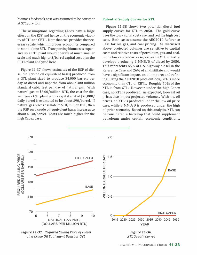
CHAPTER 11 – HYDROCARBON LIQUIDS 11-33
potential Supply curves for xtL
Figure 11-38 shows two potential diesel fuel supply curves for XTL to 2050. The gold curve uses the low capital cost case, and red the high cost case. Both cases assume the AEO2010 Reference Case for oil, gas, and coal pricing. As discussed above, projected volumes are sensitive to capital costs and relative costs of petroleum, gas, and coal. In the low capital cost case, a sizeable XTL industry develops producing 2 MMB/D of diesel by 2050. This represents 65% of U.S. highway diesel in the Reference Case and 26% of all distillate and would have a significant impact on oil imports and refin-ing. Using the AEO2010 price outlook, GTL is more economic than CTL or CBTL. Roughly 70% of the XTL is from GTL. However, under the high Capex case, no XTL is produced. As expected, forecast oil prices also impact projected volumes. With low oil prices, no XTL is produced under the low oil price case, while 3 MMB/D is produced under the high oil price scenario. Based on this analysis, XTL can be considered a backstop that could supplement petroleum under certain economic conditions.
biomass feedstock cost was assumed to be constant at $71/dry ton.
The assumptions regarding Capex have a large effect on the RSP and hence on the economic viabil-ity of CTL and CBTL. Note that coal provides the nec-essary scale, which improves economics compared to stand-alone BTL. Transporting biomass is expen-sive so a BTL plant would operate at much smaller scale and much higher $/barrel capital cost than the CBTL plant analyzed here.
Figure 11-37 shows estimates of the RSP of die-sel fuel (crude oil equivalent basis) produced from a GTL plant sized to produce 34,000 barrels per day of diesel and naphtha from about 300 million standard cubic feet per day of natural gas. With natural gas at $5.00/million BTU, the cost for die-sel from a GTL plant with a capital cost of $70,000/daily barrel is estimated to be about $90/barrel. If natural gas prices escalate to $10/million BTU, then the RSP on a crude oil equivalent basis increases to about $130/barrel. Costs are much higher for the high Capex case.
Figure 11-37. Required Selling Price of Dieselon a Crude Oil Equivalent Basis for GTL
110
150
190
230
270
HIGH CAPEX
BASE
70
NATURAL GAS PRICE(DOLLARS PER MILLION BTU)
5 6 7 8 9 10
Extra space above is for Y-axis to match others in the series 11-35, 36 & 37
RE
QU
IRE
D S
ELL
ING
PR
ICE
(DO
LLA
RS
PE
R B
AR
RE
L)
0
0.5
1.0
1.5
2.0
2015 2020 2025 2030 2035 2040 2045 2050
MIL
LIO
N B
AR
RE
LS P
ER
DA
Y
YEAR
Figure 11-38. XTL Supply Curves
HIGH CAPEX
BASE
Figure 11-37. Required Selling Price of Diesel on a Crude Oil Equivalent Basis for GTL
Figure 11-38. XTL Supply Curves

11-34 ADvANCINg TECHNOLOgY fOR AmERICA’S TRANSPORTATION fUTURE
Fuel Crude Oil Material TransportRefining Process
and Capacity
Product Distribution Pipeline/Terminal/
Outlet
Oil sandsGeographic pipeline capacity required to transport syncrude to existing refineries.
Upgrades to conventional processes required.
Drop-in
CTL – indirect
Scale to support geographic pipeline capacity likely required to transport to existing refineries.
Distillate product requires very little further processing; gasoline requires upgrade.
Drop-in
CTL – direct
Scale to support geographic pipeline capacity likely required to transport to existing refineries.
Product requires significant upgrading/ hydrotreating capacity.
Drop-in
BTL, XTL
Scale to support geographic pipeline capacity may be an issue. Truck/rail transport would be a significant logistics hurdle.
Depending on conversion process used, may range from near drop in to significant upgrade capacity required.
Drop-in
Shale
Scale to support geographic pipeline capacity may be an issue. Truck/rail transport would be a significant logistics hurdle and CO2 penalty.
Likely to require significant upgrading/ hydrogenation capacity.
Drop-in
Pyrolysis oil from bio
As-produced material may not be suitable for pipeline; on-site upgrading required. Scale to support geographic pipeline capacity may be an issue. Truck/rail transport would be a significant logistics hurdle and CO2 penalty.
Significant upgrading/ hydrogenation (oxygen rejection) capacity and technology required. Front end processing through crude units will require upgrading.
Drop-in
Renewable diesel
Scale to support geographic pipeline capacity may be an issue. Truck/rail transport would be a significant logistics hurdle and CO2 penalty.
Significant upgrading/ hydrogenation (oxygen-rejection) capacity required.
Drop-in
Biodiesel (fatty acid methyl ester)
Efficient transport, e.g. pipeline, complicated by fragmented manufacturing locations and lack of compatibility with existing hydrocarbon pipelines. Truck/rail transport would be a significant logistics hurdle and cost and CO2 penalty.
n/a
Need to address compatibility issues in existing product pipelines (jet tailback). Requires investment in terminal blending. Cold weather operational limitations.
E15-EX Ethanol
Efficient transport, e.g. pipeline, complicated by fragmented manufacturing locations and lack of compatibility with existing hydrocarbon pipelines. Truck/rail transport would be a significant logistics hurdle and cost and CO2 penalty.
n/a
Requires terminal blending. Increased E15-EX may require significant upgrades to terminal facilities for blending and storage.
Table 11-4. Alternative/Renewable Capital Infrastructure Requirements
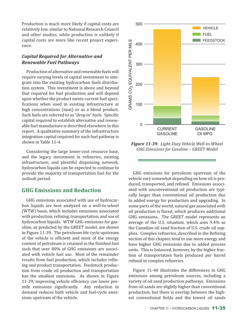
CHAPTER 11 – HYDROCARBON LIQUIDS 11-35
GHG emissions for petroleum upstream of the vehicle vary somewhat depending on how oil is pro-duced, transported, and refined. Emissions associ-ated with unconventional oil production are typi-cally larger than conventional oil production due to added energy for production and upgrading. In some parts of the world, natural gas associated with oil production is flared, which produces additional GHG emissions. The GREET model represents an average of the U.S. situation, which uses 9.4% as the Canadian oil sand fraction of U.S. crude oil sup-plies. Complex refineries, described in the Refining section of this chapter, tend to use more energy and have higher GHG emissions due to added process units. This is balanced, however, by the higher frac-tion of transportation fuels produced per barrel refined in complex refineries.
Figure 11-40 illustrates the differences in GHG emissions among petroleum sources, including a variety of oil sand production pathways. Emissions from oil sands are slightly higher than conventional production, but there is overlap between the high-est conventional fields and the lowest oil sands
Production is much more likely if capital costs are relatively low, similar to National Research Council and other studies, while production is unlikely if capital costs are more like recent project experi-ence.
Capital Required for Alternative and Renewable Fuel Pathways
Production of alternative and renewable fuels will require varying levels of capital investment to inte-grate into the existing hydrocarbon fuels distribu-tion system. This investment is above and beyond that required for fuel production and will depend upon whether the product meets current fuel speci-fications when used in existing infrastructure at high concentrations (neat) or as a blend product. Such fuels are referred to as “drop in” fuels. Specific capital required to establish alternative and renew-able fuel manufacture is described elsewhere in this report. A qualitative summary of the infrastructure integration capital required for each fuel pathway is shown in Table 11-4.
Considering the large lower-cost resource base, and the legacy investment in refineries, existing infrastructure, and plentiful dispensing network, hydrocarbon liquids can be expected to continue to provide the majority of transportation fuel for the outlook period.
GHG Emissions and reduction
GHG emissions associated with use of hydrocar-bon liquids are best analyzed on a well-to-wheel (WTW) basis, which includes emissions associated with production, refining, transportation, and use of hydrocarbon liquids. WTW GHG emissions for gas-oline, as predicted by the GREET model, are shown in Figure 11-39. The petroleum life-cycle upstream of the vehicle is efficient and most of the energy content of petroleum is retained in the finished fuel such that over 80% of GHG emissions are associ-ated with vehicle fuel use. Most of the remainder results from fuel production, which includes refin-ing and product transportation. Feedstock produc-tion from crude oil production and transportation has the smallest emissions. As shown in Figure 11-39, improving vehicle efficiency can lower per-mile emissions significantly. Any reduction in demand reduces both vehicle and fuel-cycle emis-sions upstream of the vehicle.
0
100
200
300
400
500
GASOLINE2X MPG
CURRENTGASOLINE
GR
AM
S C
O2
EQ
UIV
ALE
NT
PE
R M
ILE
Figure 11-39. Light-Duty Vehicle Well-to-WheelsGHG Emissions for Gasoline – GREET Model
VEHICLE
FUEL
FEEDSTOCK
Figure 11-39. Light-Duty Vehicle Well-to-Wheel GHG Emissions for Gasoline – GREET Model

11-36 ADvANCINg TECHNOLOgY fOR AmERICA’S TRANSPORTATION fUTURE
a capacity of 14.6 gigawatts.17 While CHP systems are already in use at the majority of the 145 U.S. refineries, there are opportunities to add CHP or to repower existing plants making them larger and more efficient.
Increased biofuel blending can lower transpor-tation GHG depending on the source of the biofuel. Low-level biofuel blends leverage the existing fuel distribution and vehicle infrastructure, provid-ing an advantage compared to alternatives that require a new infrastructure. There are no major technical limitations to increased biofuel use, but significant investments in distribution and vehicle infrastructure will be needed depending on the biofuel produced.
Carbon sequestration could produce reduc-tions in GHG emissions from refinery and thermal oil production but is expected to be very costly.
17 U.S. Environmental Protection Agency, Office of Air Quality Planning and Standards, Available and Emerging Technologies for Reducing Greenhouse Gas Emissions from the Petroleum Refining Industry, October 2010.
pathways. Some conventional fields have emis-sions that are similar to oil sands.
GHG Reduction in Petroleum Pathway
According to a 2010 EPA report, although the potential for reducing emissions in the hydro-carbon liquid supply chain is relatively small compared to the fuel carbon content, there are emission reduction strategies for refining. Most options improve efficiency and reduce energy use. As discussed previously, there has been an ongo-ing improvement in refining energy efficiency. Further improvement could come from more effi-cient combustion, equipment (pumps, compres-sors, etc.) and lighting, reduced heat losses, and a variety of other measures. Generally, these items are small individually and so must be approached in a systematic manner, hence the value of energy management systems, which are already widely in use in refining. The large steam requirements for refining operations make refineries excellent candidates for combined heat and power (CHP). Refineries represent one of the largest industry sources of CHP today, with 103 active plants with
Figure 11-40. Well to Wheels Emissions for Selected Crude Oils
0
40
80
120
BACHA-QUERO
MAYA MARS KIRKUK
ARABMEDIUM
BONNYLIGHT
CATHERMAL
EORSAGD
SYNTHETIC
SAGDSYNTHETIC
COKER SAGD
BITUMEN
DILBIT MININGBITUMEN
MININGSYNTHETIC
Figure 11-40. Well-to-Wheels GHG Emissions for Selected Crudes Refined to Reformulated Gasoline
REFINING/UPGRADING
Note: g/MJ measures the grams of CO2 equivalent GHGs emitted per megajoule of reformulated gasoline consumed, after accounting for all emissions from producing and refining the crude or bitumen into reformulated gasoline blending stock, plus all emissions from transporting the gasoline to the sevice station, and burning the gasoline in vehicles.
Sources: The Conference Board of Canada; Alberta Innovates – Energy and Environment Solutions.
GR
AM
S C
O2
EQ
UIV
ALE
NT
P
ER
ME
GA
JOU
LEVEHICLE PRODUCTION/TRANSPORT TO REFINERY

CHAPTER 11 – HYDROCARBON LIQUIDS 11-37
sions of petroleum-derived fuel. Petroleum ratio greater than 1.0 indicates XTL pathways with GHG emissions higher than petroleum, and petroleum ratio less than 1.0 indicates XTL pathways with lower emissions than petroleum. Without seques-tration, GTL and especially CTL have higher emis-sions than petroleum due to higher energy use in fuel production and in the case of coal higher fuel carbon content. However, since XTL produces a concentrated stream of CO2, sequestration would be more cost-effective compared to utility sources. In this case, XTL can have GHG emissions lower than petroleum. Use of biomass in CBTL provides a small additional reduction relative to CTL with or without CCS; however, the reduction is limited by the small 15% fraction of biomass to the total CBTL feedstock cost.
Transportation 2050 Discussion
As discussed above, demand reduction can pro-duce the largest reductions of GHG in the hydro-carbon liquid pathway. To illustrate the potential benefits and to discuss potential issues, an alterna-tive scenario was developed with reduced demand based on improved vehicle efficiency. The scenario was based on a target of 50% improvement in light-duty and 25% improvement in heavy-duty fuel effi-ciency per vehicle mile traveled (VMT) by 2050.20 As expected, the alternative scenario produced a 23–27% reduction in highway vehicle energy, petroleum use, and GHG compared to the refer-ence case. (See Table 11-6 and Figures 11-41 and 11-42.) The largest reductions were in light-duty vehicle GHG emissions, consistent with the greater improvement in vehicle efficiency. By 2050,
20 Laboratory for Energy and Environment, MIT, Factor of Two: Halving the Fuel Consumption of New US Automobiles by 2035, 2007; USEPA, NHTSA, CARB, Interim Joint Technical Assessment Report: Light-Duty Vehicle Greenhouse Gas Emission Standards and Corporate Average Fuel Economy Standards for Model years 2017-2025, September 2010; and USEPA and NHTSA, Draft Regulatory Impact Analysis, Proposed Rulemaking to Establish Greenhouse Gas Emissions Standards and Fuel Efficiency Standards for Medium- and Heavy-Duty Engines and Vehicles, October 2010.
Current cost estimates for electric power plant coal CCS for the Nth-of-a-kind plant are $60–$100/ton of CO2 avoided.18 CCS for refining emissions is expected to be significantly more costly than power generation CCS because the CO2 streams are typically smaller scale and more widely dis-tributed than those from large power plants. Car-bon sequestration may be more easily applied to GTL and other non-petroleum pathways, however, due to the presence of a concentrated CO2 stream as discussed below.
GHG produced in transportation of crude oil and petroleum products are best addressed by using the most efficient transportation modes, which are marine and pipeline. As previously discussed, most petroleum transportation is already by these modes. Increased use of trucks to accommodate biofuels or other new fuels could increase GHG, however.
Gasoline Octane
Increased gasoline octane can improve vehicle fuel economy by allowing use of higher engine com-pression ratio. Only new vehicles that are designed for the higher octane would benefit significantly. Producing higher octane increases energy use and GHG emissions in refineries. The overall effect of changing octane should be evaluated on a WTW basis that includes both vehicle and refinery effects. A WTW study in Japan found a net increase in vehi-cle plus refinery GHG for an octane increase from 90 to 95 RON (research octane number).19
XTL GHG Emissions
Table 11-5 lists the petroleum ratio for a variety of XTL pathways. The petroleum ratio is defined as the life-cycle GHG emissions of producing and using the XTL fuel divided by the life-cycle emis-
18 H. S. Kheshgi, et al., “Perspectives on CCS Cost and Economics,” SPE International Conference on CO2 Capture, Storage, and Utilization, New Orleans, LA, November 2010.
19 Japan Clean Air Program (JCAP). 4th JCAP Conference, June 1, 2005, Session 2; and 5th JCAP Conference, February 22, 2007, Session 1.
TechnologyCTL
(No CCS)CTL
(CCS)CBTL*
(No CCS)CBTL* (CCS)
GTL (No CCS)
GTL (CCS)
Petroleum Ratio ~2.2 ~0.9-1.0 ~1.9 ~0.8-0.9 ~1.1 ~0.9
* CBTL plants co-feed 15 weight % biomass.
Table 11-5. Life-Cycle GHG Emissions for XTL Relative to Petroleum

11-38 ADvANCINg TECHNOLOgY fOR AmERICA’S TRANSPORTATION fUTURE
light-duty vehicle GHG emissions were 22% lower than 2010. (See Figure 11-43 for highway vehi-cle GHG emissions in both cases.) The efficiency gains also result in a large decrease in petroleum imports, approximately 4 MMB/D below the ref-erence case. The reference and alternative cases were based on the AEO2010. The more recent AEO2012 Early Release is projecting roughly 20% less VMT than the AEO2010. Combining the slower VMT growth in the more recent projection with improved vehicle fuel economy would pro-duce even larger reductions in energy use, GHG, and petroleum imports. Even larger GHG reduc-tions could be achieved by the following: increase vehicle efficiency further; change vehicle power, size, or other characteristics; reduce the growth in highway VMT; fuel substitution; or reduced GHG in the petroleum pathway.
Note that the alternative case only considered highway vehicles. Inclusion of non-highway vehi-cles would dilute the percentage improvement val-ues. Modal substitution, increased efficiency, and fuel substitution are potential measures for air, rail, and marine sectors.
Figure 11-41. Highway Vehicle Fuel Use – Reference Case (Based on AEO2010)
0
4
8
12
16
2000 2010 2020 2030 2040 2050
MIL
LIO
NS
OF
BA
RR
ELS
PE
R D
AY
YEAR
Figure 11-41. Highway Vehicle Fuel Use – Reference Case (Based on AEO2010)
XTL DIESEL
BIODIESEL
ETHANOL
DIESEL
GASOLINE
2010Refer-ence 2050
Alter-native 2050
Delta Ref.-->
Alt.
Energy Use % Relative 2010
– +33% -2% -26%
Petroleum Use % Relative 2010
– +15% -12% -23%
GHG (million metric tons)
– +28% -6% -27%
% Gasoline of Petro-leum
80 73 65 -11%
% Ethanol in Gasoline Pool
9.5 18 25 +37%
Table 11-6. Highway Vehicle Metrics – Reference and Alternative Cases
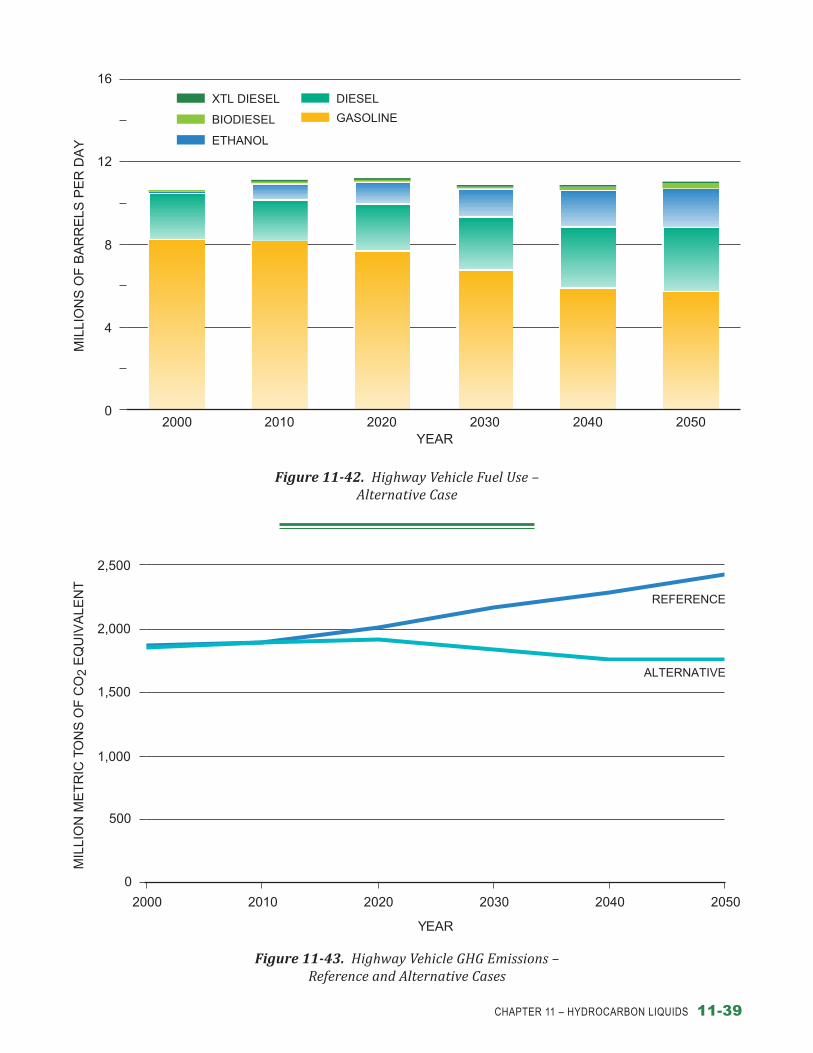
CHAPTER 11 – HYDROCARBON LIQUIDS 11-39
Figure 11-42. Highway Vehicle Fuel Use – Alternative Case
Figure 11-42. Highway Vehicle Fuel Use – Alternative Case
0
4
8
12
16
2000 2010 2020 2030 2040 2050
MIL
LIO
NS
OF
BA
RR
ELS
PE
R D
AY
YEAR
XTL DIESEL
BIODIESEL
ETHANOL
DIESEL
GASOLINE
0
500
1,000
1,500
2,000
2,500
2000 2010 2020 2030 2040 2050
MIL
LIO
N M
ET
RIC
TO
NS
OF
CO
2 E
QU
IVA
LEN
T
YEAR
Figure 11-43. Highway Vehicle GHG Emissions – Reference and Alternative Cases
REFERENCE
ALTERNATIVE
Figure 11-43. Highway Vehicle GHG Emissions – Reference and Alternative Cases

11-40 ADvANCINg TECHNOLOgY fOR AmERICA’S TRANSPORTATION fUTURE
Iandoli, Carmine L., and Signe Kjelstrup. “Exergy Analysis of a GTL Process Based on Low-Temperature Slurry F-T Reactor Technology with a Cobalt Catalyst,” Energy Fuels 21, no. 4 (2007): pages 2317-2324. http://www.chem.ntnu.no/non equilibrium-thermodynamics/pub/176-Iandoli-EnergyFuels.pdf.
International Energy Agency. World Energy Outlook 2008. 2008.
International Energy Agency. World Energy Outlook 2010. 2010.
Japan Clean Air Program (JCAP). 4th JCAP Confer-ence, June 1, 2005, Session 2 “3. CO2 Emissions Study Workgroup Report.” http://www.pecj.or.jp/english/jcap/jcap2/jcap2_4th.html.
Japan Clean Air Program (JCAP). 5th JCAP Con-ference, February 22, 2007, Session 1, “2. Gaso-line Work Group Report.” http://www.pecj.or.jp/ english/jcap/jcap2/jcap2_5th.html.
Jessen, Holly. “Riding the Rails.” Ethanol Producer Magazine. October 2006.
Kheshgi, Haroon S., Hans Thomann, Nazeer A. Bhore, Robert B. Hirsch, Michael E. Parker, and Gary Teletzke. “Perspectives on CCS Cost and Econom-ics,” SPE International Conference on CO2 Capture, Storage, and Utilization, New Orleans, LA. Novem-ber 2010.
Laboratory for Energy and Environment, MIT, Fac-tor of Two: Halving the Fuel Consumption of New US Automobiles by 2035, 2007.
National Academy of Sciences, National Academy of Engineering, and National Research Council of the National Academies, Liquid Transportation Fuels from Coal and Biomass: Technological Status, Costs, and Environmental Impacts. 2009.
National Association of Convenience Stores. Chal-lenges Remain Before E15 Usage is Widespread. 2011. http://www.nacsonline.com/NACS/Resources/campaigns/GasPrices_2011/Pages/ChallengesRemainBeforeE15UsageIsWidespread.aspx.
Alberta Energy Research Institute. Life Cycle Emis-sion Comparison of North American and Imported Crudes. Prepared by Jacobs Consultancy and Life-cycle Associates, July 2009.
American Petroleum Institute. API RFS2 Comments, Attachment 4: E85 Retail Fueling Cost Study. 2009.
Association of Oil Pipe Lines and American Petro-leum Institute. “In the Pipe” (newsletter). April 2006.
Association of Oil Pipe Lines. Liquid Pipeline Indus-try in the United States, Where It’s Been: Where It’s Going. April 2004.
Association of Oil Pipe Lines. Report on Shifts in Petroleum Transportation: 1990–2009. Febru-ary 2012. http://www.aopl.org/pdf/AOPL_Shift_Report_Press_Release_Feb_7_20121.pdf.
Borensztein, Eduardo, and Carmen M. Reinhart. The Macroeconomic Determinants of Commodity Prices. University of Maryland. 1994.
BP. BP Statistical Review of World Energy. June 2011.
Clean Fuels Foundation and the Nebraska Ethanol Board. In cooperation with the U.S. Department of Agriculture. E85 and Blender Pumps: A Resource Guide to Ethanol Refueling Infrastructure. 2011.
CME Group. The Role of WTI as a Crude Oil Bench-mark. January 2010.
The Conference Board of Canada. “Getting the Bal-ance Right: The Oil Sands, Exporting and Sustain-ability.” Briefing January 2010.
Congressional Research Service. Intermediate-Level Blends of Ethanol in Gasoline, and the Ethanol “Blend Wall.” October 2010.
Congressional Research Service. The U.S. Oil Refin-ing Industry: Background in Changing Markets and Fuel Policies. November 2010.
Europia. “White Paper on EU Refining.” 2011.
GREET Model: The Greenhouse Gases, Regulated Emissions, and Energy Use in Transportation Model, Argonne National Laboratory. http://greet.es.anl.gov/.
bibLioGrapHy

CHAPTER 11 – HYDROCARBON LIQUIDS 11-41
U.S. Energy Information Administration. Annual Energy Outlook 2010—With Projections to 2035. April 2010.
U.S. Energy Information Administration. Annual Energy Outlook 2011—With Projections to 2035. April 2011.
U.S. Energy Information Administration. Annual Energy Outlook 2012 Early Release. December 2011.
U.S. Environmental Protection Agency, and National Highway Traffic Safety Administra-tion. Draft Regulatory Impact Analysis, Proposed Rulemaking to Establish Greenhouse Gas Emis-sions Standards and Fuel Efficiency Standards for Medium- and Heavy-Duty Engines and Vehicles, October 2010. http://www.epa.gov/otaq/climate/regulations/420d10901.pdf.
U.S. Environmental Protection Agency, National Highway Traffic Safety Administration, and Cali-fornia Air Resources Board. Interim Joint Technical Assessment Report: Light-Duty Vehicle Greenhouse Gas Emission Standards and Corporate Average Fuel Economy Standards for Model years 2017-2025. Sep-tember 2010. http://www.epa.gov/otaq/climate/regulations/ldv-ghg-tar.pdf.
U.S. Environmental Protection Agency, Office of Air Quality Planning and Standards. Available and Emerging Technologies for Reducing Greenhouse Gas Emissions from the Petroleum Refining Industry. October 2010.
U.S. Environmental Protection Agency. Draft Regu-latory Impact Analysis: Changes to Renewable Fuel Standard Program, Section 4.2.1.1.6. May 2009.
Valero (website), Industry Fundamentals. “Basics of Refining and Coking.” January 2011. http://www.valero.com/InvestorRelations/Pages/Industry Fundamentals.aspx.
Zeus Intelligence, Zeus Syngas Refining Report, March 1, 2011. Similar estimates have been pub-lished.
National Energy Technology Laboratory and U.S. Department of Energy, Affordable, Low-Carbon Diesel Fuel from Domestic Coal and Biomass, DOE/NETL 2009/1349. 2009.
National Petroleum Council. “Appendix C: History and Fundamentals of Refining Operations.” In U.S. Petroleum Refining. June 2000.
National Petroleum Council. “Appendix D: The U.S. Petroleum Distribution System (A Tutorial).” In U.S. Petroleum Refining. June 2000.
National Petroleum Council. Hard Truths: Facing the Hard Truths about Energy. 2007.
National Petroleum Council. Prudent Development: Realizing the Potential for North America’s Abun-dant Natural Gas and Oil Resources. 2011.
National Petroleum Council. U.S. Petroleum Refining – Assuring the Adequacy and Affordability of Cleaner Fuels. 2000.
Petroleum Equipment Institute. Compatibility Assessment Survey. 2008.
Shell (website). “Pearl GTL: An Overview.” 2011. http://www.shell.com/home/content/aboutshell/our_strategy/major_projects_2/pearl/overview/, and references in that website.
Solomon Associates, private communication.
U.S. Department of Energy, Alternative Fuels Data Center (website). “Propane.” http://www.afdc.energy.gov/vehicles/propane.html.
U.S. Department of Energy, Oak Ridge National Lab-oratory, “Chapter 4” in Transportation Energy Data Book. http://cta.ornl.gov/data/chapter4.shtml.
U.S. Energy Information Administration. “Atlantic Basin Refining Dynamics from U.S. Perspective.” Presentation by Joanne Shore and John Hackworth at Platts 4th Annual European Refining Markets Conference, September 2010.