event scheduling using constraint programming november 22, 2002 martin henz, school of computing,...
TRANSCRIPT
Event Scheduling Using Constraint Programming
November 22, 2002
Martin Henz, School of Computing, NUSwww.comp.nus.edu.sg/~henz/sma2002
SMA / CS © NUS 2002 2
Overview
Constraint programming in a nutshell Elements of constraint programming Sport tournament scheduling Production scheduling Assessment
SMA / CS © NUS 2002 3
Overview
Constraint programming in a nutshell Elements of constraint programming Sport tournament scheduling Production scheduling Assessment
SMA / CS © NUS 2002 4
Constraint Programming in a Nutshell
SEND MORE MONEY
SMA / CS © NUS 2002 5
Constraint Programming in a Nutshell
SEND + MORE = MONEY
SMA / CS © NUS 2002 6
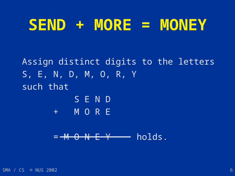
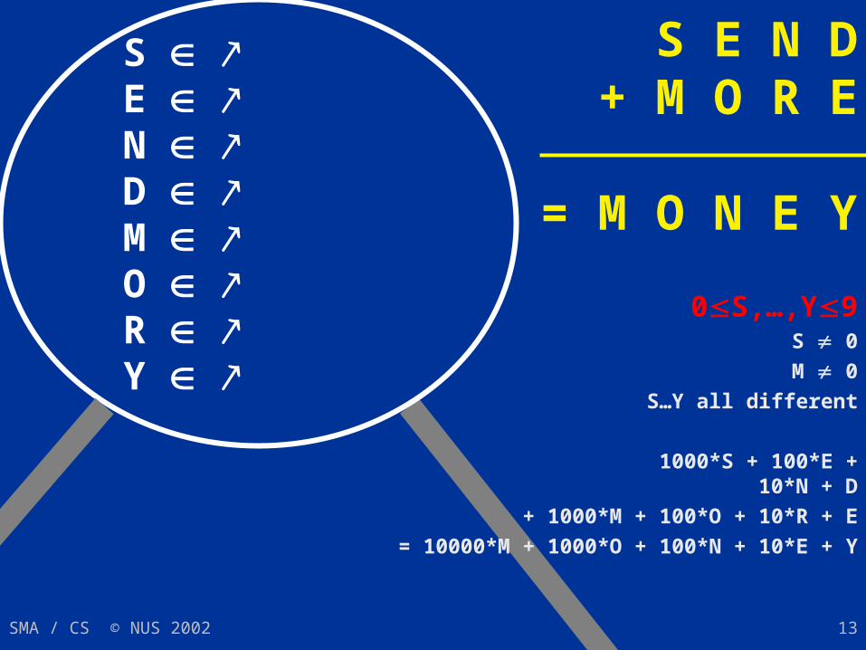
SEND + MORE = MONEY
Assign distinct digits to the letters
S, E, N, D, M, O, R, Y
such that
S E N D
+ M O R E
= M O N E Y holds.
SMA / CS © NUS 2002 7
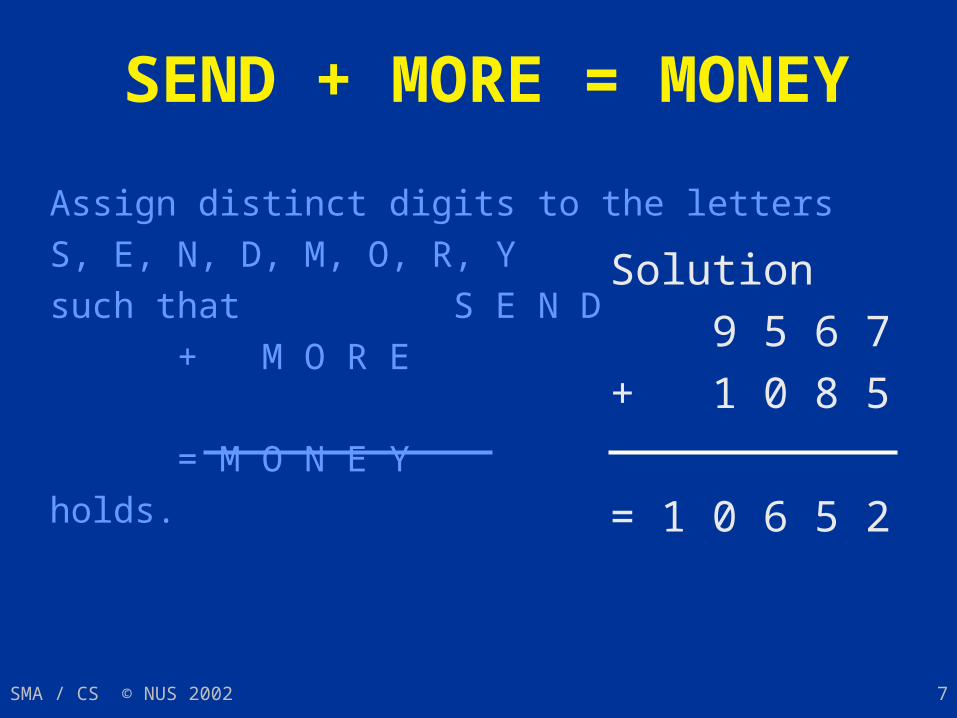
SEND + MORE = MONEY
Assign distinct digits to the letters
S, E, N, D, M, O, R, Y
such that S E N D
+ M O R E
= M O N E Y
holds.
Solution
9 5 6 7
+ 1 0 8 5
= 1 0 6 5 2
SMA / CS © NUS 2002 8
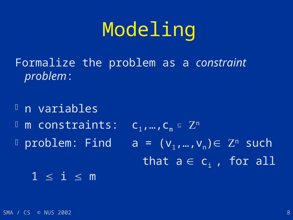
Modeling
Formalize the problem as a constraint problem:
n variables m constraints: c1,…,cm
n
problem: Find a = (v1,…,vn) n such
that a ci , for all 1 i m
SMA / CS © NUS 2002 9
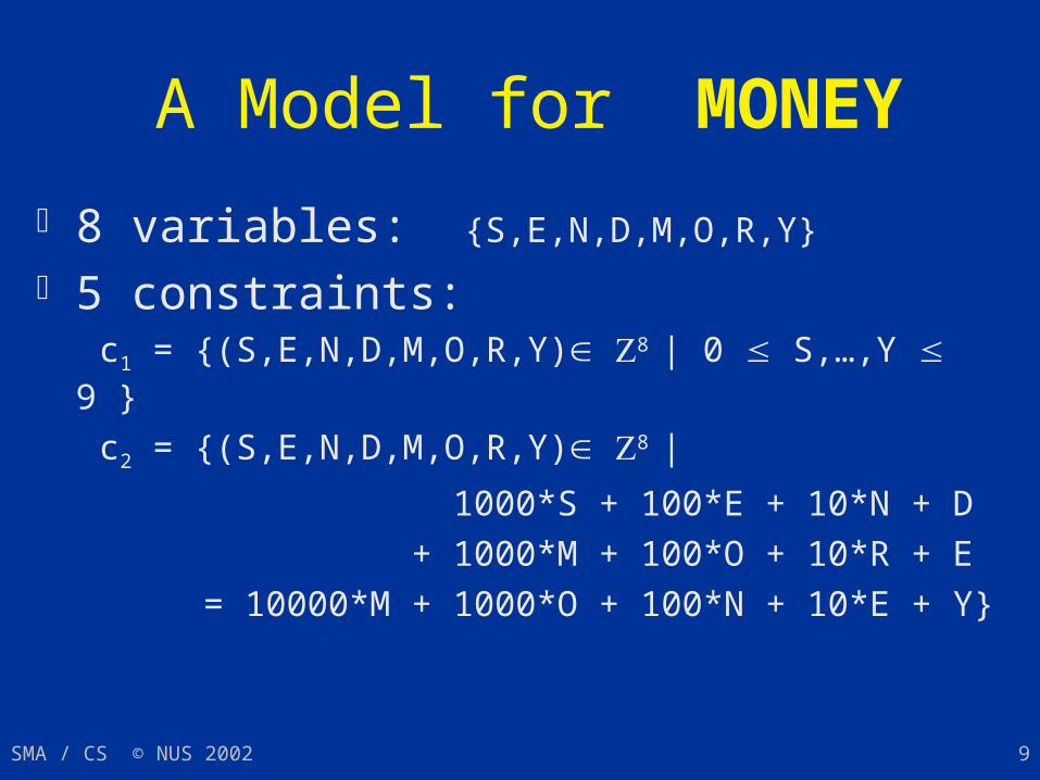
A Model for MONEY
8 variables: {S,E,N,D,M,O,R,Y} 5 constraints: c1 = {(S,E,N,D,M,O,R,Y) 8 | 0 S,…,Y 9 }
c2 = {(S,E,N,D,M,O,R,Y) 8 |
1000*S + 100*E + 10*N + D
+ 1000*M + 100*O + 10*R + E
= 10000*M + 1000*O + 100*N + 10*E + Y}
SMA / CS © NUS 2002 10
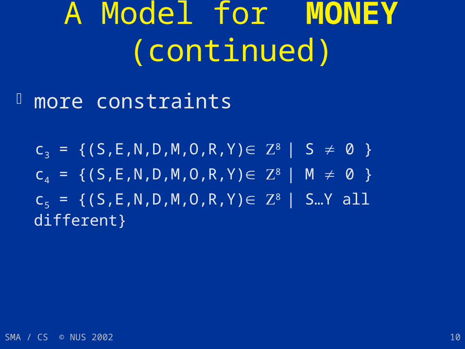
A Model for MONEY (continued) more constraints
c3 = {(S,E,N,D,M,O,R,Y) 8 | S 0 }
c4 = {(S,E,N,D,M,O,R,Y) 8 | M 0 }
c5 = {(S,E,N,D,M,O,R,Y) 8 | S…Y all different}
SMA / CS © NUS 2002 11
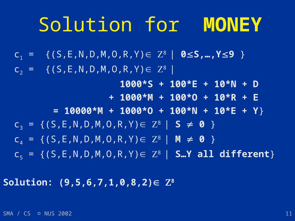
Solution for MONEY c1 = {(S,E,N,D,M,O,R,Y) 8 | 0S,…,Y9 }
c2 = {(S,E,N,D,M,O,R,Y) 8 |
1000*S + 100*E + 10*N + D
+ 1000*M + 100*O + 10*R + E
= 10000*M + 1000*O + 100*N + 10*E + Y}
c3 = {(S,E,N,D,M,O,R,Y) 8 | S 0 }
c4 = {(S,E,N,D,M,O,R,Y) 8 | M 0 }
c5 = {(S,E,N,D,M,O,R,Y) 8 | S…Y all different}
Solution: (9,5,6,7,1,0,8,2) 8
SMA / CS © NUS 2002 12
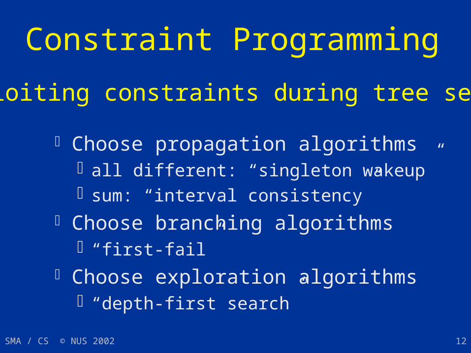
Constraint Programming
Choose propagation algorithms all different: “singleton wakeup” sum: “interval consistency”
Choose branching algorithms “first-fail”
Choose exploration algorithms “depth-first search”
Exploiting constraints during tree search
SMA / CS © NUS 2002 13
S E N D+ M O R E
= M O N E Y
0S,…,Y9 S 0M 0
S…Y all different
1000*S + 100*E + 10*N + D
+ 1000*M + 100*O + 10*R + E
= 10000*M + 1000*O + 100*N + 10*E + Y
S E N D M O R Y
SMA / CS © NUS 2002 14
S E N D+ M O R E
= M O N E Y
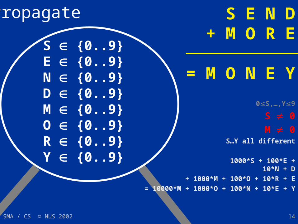
0S,…,Y9
S 0M 0
S…Y all different
1000*S + 100*E + 10*N + D
+ 1000*M + 100*O + 10*R + E
= 10000*M + 1000*O + 100*N + 10*E + Y
S {0..9}E {0..9}N {0..9}D {0..9}M {0..9}O {0..9}R {0..9}Y {0..9}
Propagate
SMA / CS © NUS 2002 15
S E N D+ M O R E
= M O N E Y
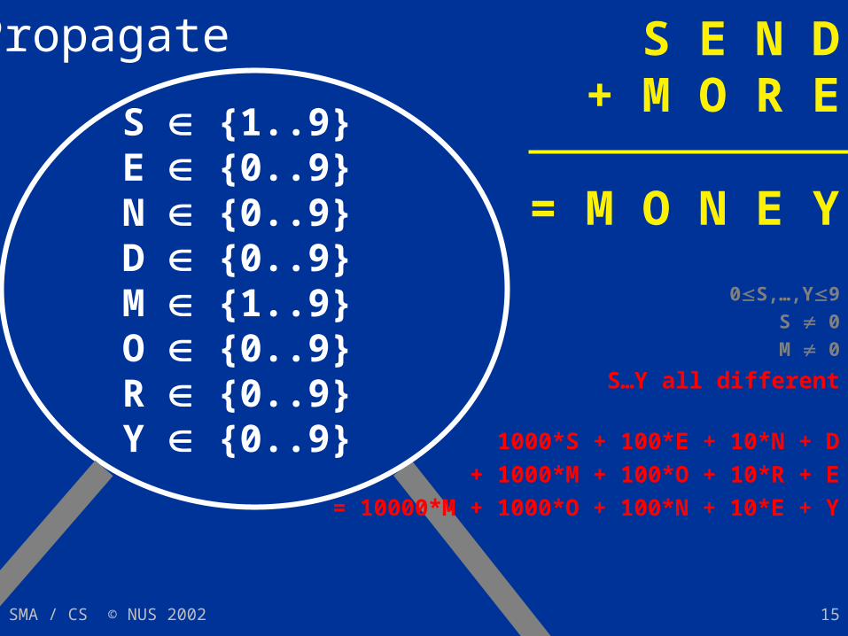
0S,…,Y9 S 0M 0
S…Y all different
1000*S + 100*E + 10*N + D
+ 1000*M + 100*O + 10*R + E
= 10000*M + 1000*O + 100*N + 10*E + Y
S {1..9}E {0..9}N {0..9}D {0..9}M {1..9}O {0..9}R {0..9}Y {0..9}
Propagate
SMA / CS © NUS 2002 16
S E N D+ M O R E
= M O N E Y
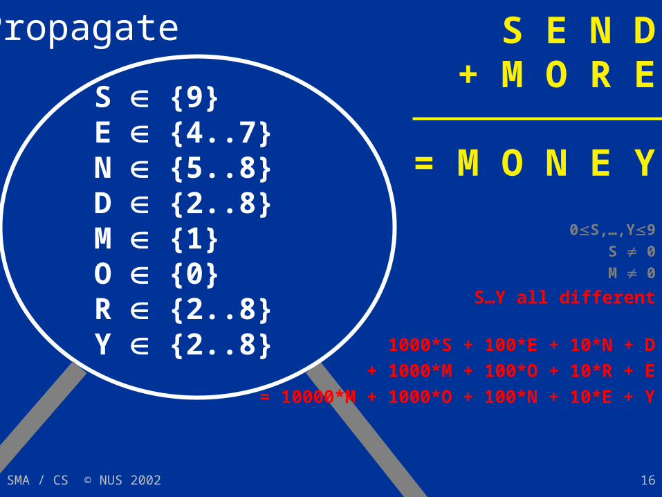
0S,…,Y9 S 0M 0
S…Y all different
1000*S + 100*E + 10*N + D
+ 1000*M + 100*O + 10*R + E
= 10000*M + 1000*O + 100*N + 10*E + Y
S {9}E {4..7}N {5..8}D {2..8}M {1}O {0}R {2..8}Y {2..8}
Propagate
SMA / CS © NUS 2002 17
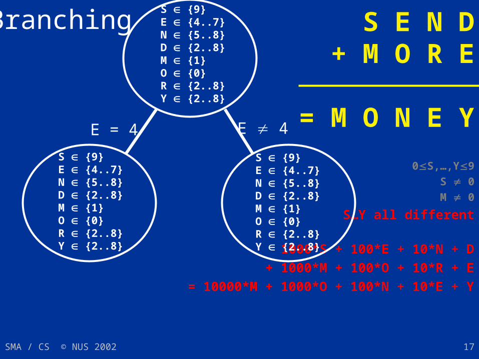
S E N D+ M O R E
= M O N E Y
0S,…,Y9 S 0M 0
S…Y all different
1000*S + 100*E + 10*N + D
+ 1000*M + 100*O + 10*R + E
= 10000*M + 1000*O + 100*N + 10*E + Y
S {9}E {4..7}N {5..8}D {2..8}M {1}O {0}R {2..8}Y {2..8}
S {9}E {4..7}N {5..8}D {2..8}M {1}O {0}R {2..8}Y {2..8}
S {9}E {4..7}N {5..8}D {2..8}M {1}O {0}R {2..8}Y {2..8}
E = 4 E 4
Branching
SMA / CS © NUS 2002 18
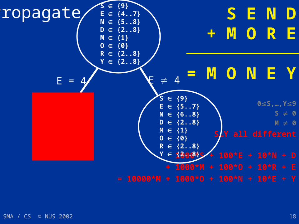
S E N D+ M O R E
= M O N E Y
0S,…,Y9 S 0M 0
S…Y all different
1000*S + 100*E + 10*N + D
+ 1000*M + 100*O + 10*R + E
= 10000*M + 1000*O + 100*N + 10*E + Y
S {9}E {4..7}N {5..8}D {2..8}M {1}O {0}R {2..8}Y {2..8}
S {9}E {5..7}N {6..8}D {2..8}M {1}O {0}R {2..8}Y {2..8}
E = 4 E 4
Propagate
SMA / CS © NUS 2002 19
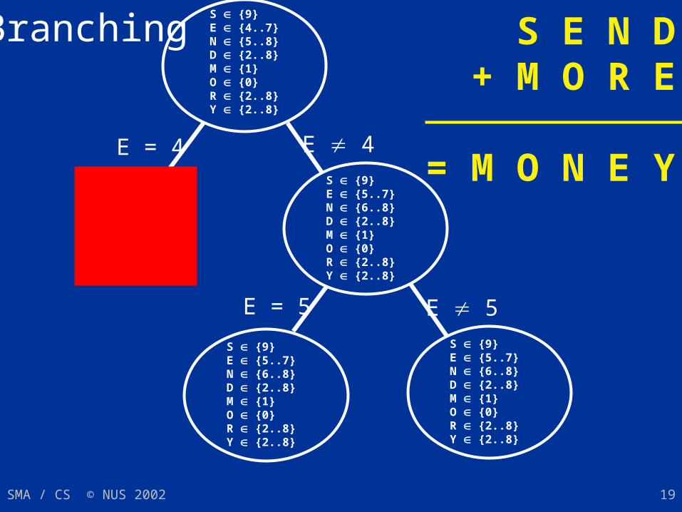
S E N D+ M O R E
= M O N E Y
S {9}E {4..7}N {5..8}D {2..8}M {1}O {0}R {2..8}Y {2..8}
S {9}E {5..7}N {6..8}D {2..8}M {1}O {0}R {2..8}Y {2..8}
E = 4 E 4
Branching
S {9}E {5..7}N {6..8}D {2..8}M {1}O {0}R {2..8}Y {2..8}
E = 5 E 5
S {9}E {5..7}N {6..8}D {2..8}M {1}O {0}R {2..8}Y {2..8}
SMA / CS © NUS 2002 20
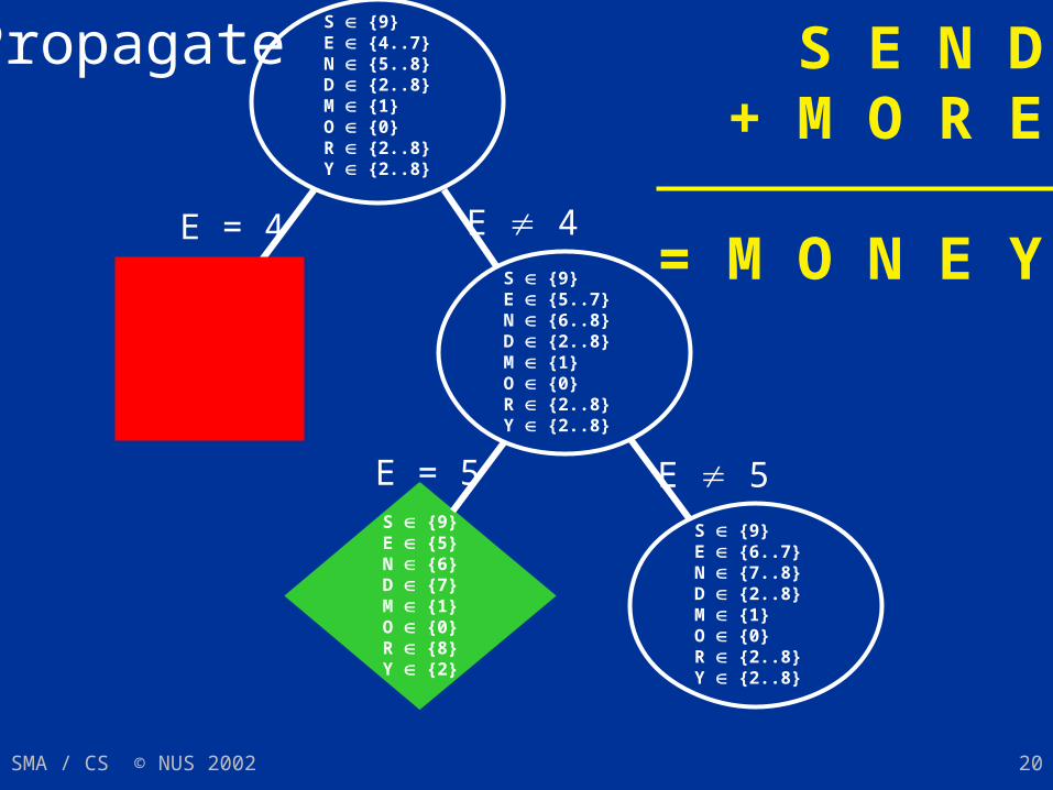
S E N D+ M O R E
= M O N E Y
S {9}E {4..7}N {5..8}D {2..8}M {1}O {0}R {2..8}Y {2..8}
S {9}E {5..7}N {6..8}D {2..8}M {1}O {0}R {2..8}Y {2..8}
E = 4 E 4
Propagate
S {9}E {6..7}N {7..8}D {2..8}M {1}O {0}R {2..8}Y {2..8}
E = 5 E 5S {9}E {5}N {6}D {7}M {1}O {0}R {8}Y {2}
SMA / CS © NUS 2002 21
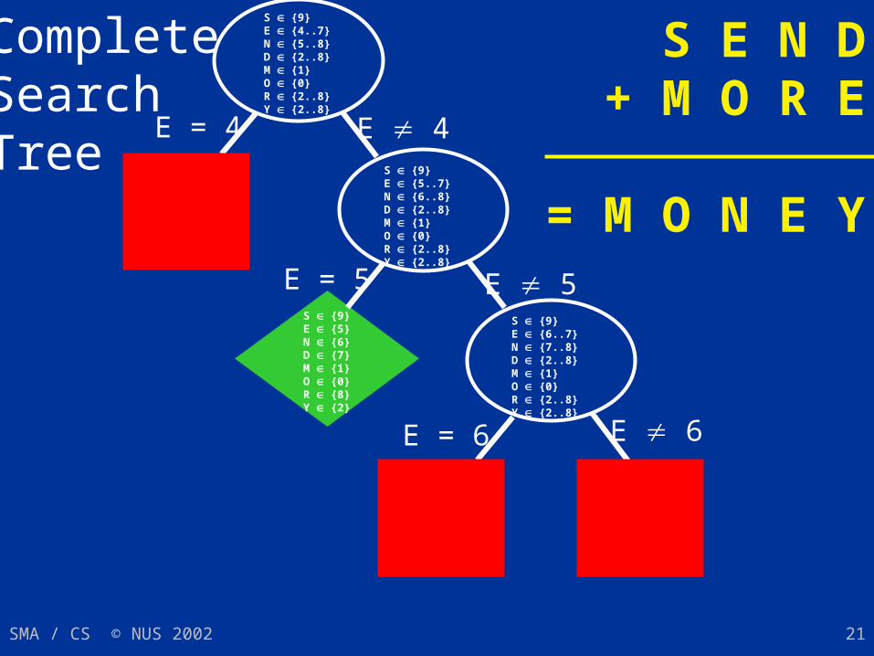
S E N D+ M O R E
= M O N E Y
CompleteSearchTree
S {9}E {4..7}N {5..8}D {2..8}M {1}O {0}R {2..8}Y {2..8}
S {9}E {5..7}N {6..8}D {2..8}M {1}O {0}R {2..8}Y {2..8}
E = 4 E 4
S {9}E {6..7}N {7..8}D {2..8}M {1}O {0}R {2..8}Y {2..8}
E = 5 E 5S {9}E {5}N {6}D {7}M {1}O {0}R {8}Y {2}
E = 6 E 6
SMA / CS © NUS 2002 22
The Art of Constraint Programming
Choose model Choose propagation algorithms Choose branching algorithms Choose exploration algorithms
SMA / CS © NUS 2002 23
Demo: SEND + MORE = MONEY
Click here for MONEY
SMA / CS © NUS 2002 24
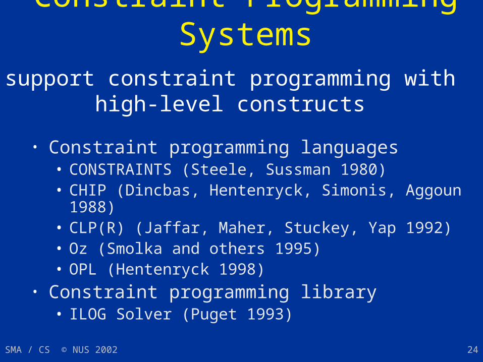
Constraint Programming Systems
• Constraint programming languages• CONSTRAINTS (Steele, Sussman 1980)• CHIP (Dincbas, Hentenryck, Simonis, Aggoun 1988)• CLP(R) (Jaffar, Maher, Stuckey, Yap 1992)• Oz (Smolka and others 1995)• OPL (Hentenryck 1998)
• Constraint programming library• ILOG Solver (Puget 1993)
support constraint programming withhigh-level constructs
SMA / CS © NUS 2002 25
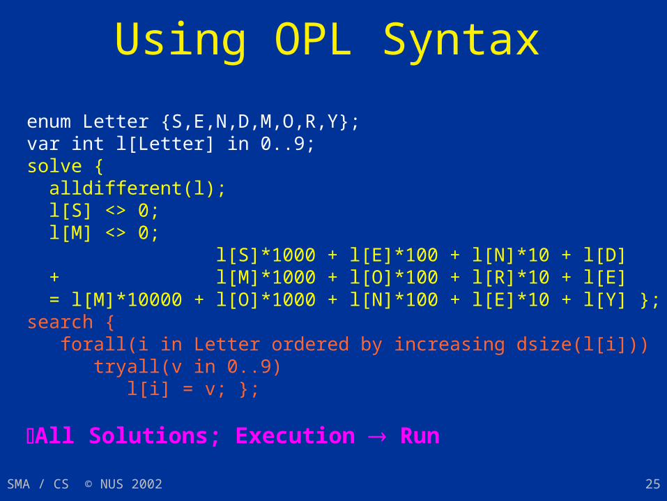
Using OPL Syntax
enum Letter {S,E,N,D,M,O,R,Y};var int l[Letter] in 0..9;solve { alldifferent(l); l[S] <> 0; l[M] <> 0; l[S]*1000 + l[E]*100 + l[N]*10 + l[D] + l[M]*1000 + l[O]*100 + l[R]*10 + l[E] = l[M]*10000 + l[O]*1000 + l[N]*100 + l[E]*10 + l[Y] };search { forall(i in Letter ordered by increasing dsize(l[i])) tryall(v in 0..9) l[i] = v; };
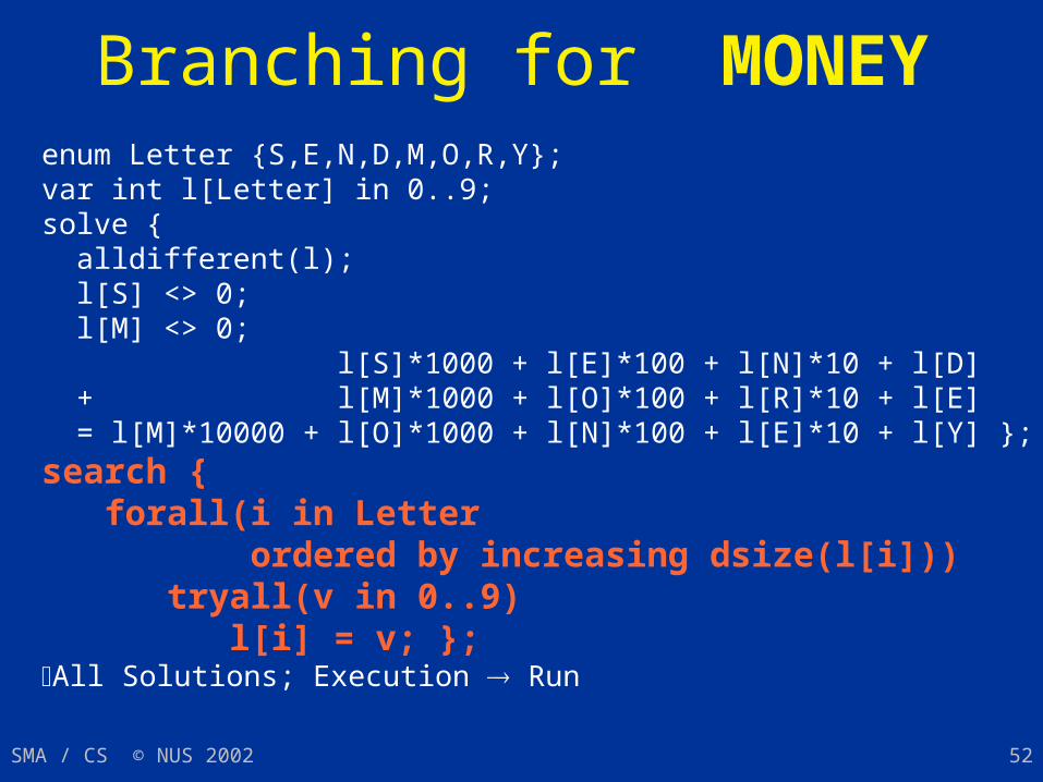
All Solutions; Execution Run
SMA / CS © NUS 2002 26
Overview
Constraint programming in a nutshell Elements of constraint programming Sport tournament scheduling Production scheduling Assessment
SMA / CS © NUS 2002 27
Elements of Constraint Programming
The Approach Propagation Branching Exploration
SMA / CS © NUS 2002 28
Elements of Constraint Programming
The Approach Propagation Branching Exploration
SMA / CS © NUS 2002 29
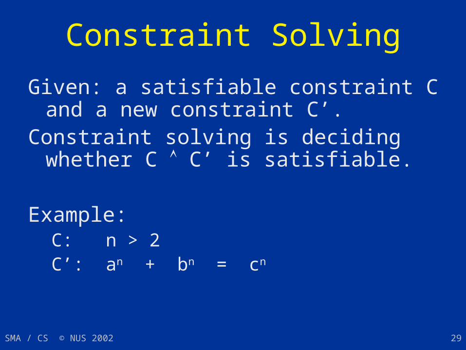
Constraint Solving
Given: a satisfiable constraint C and a new constraint C’.
Constraint solving is deciding whether C C’ is satisfiable.
Example: C: n > 2C’: an + bn = cn
SMA / CS © NUS 2002 30
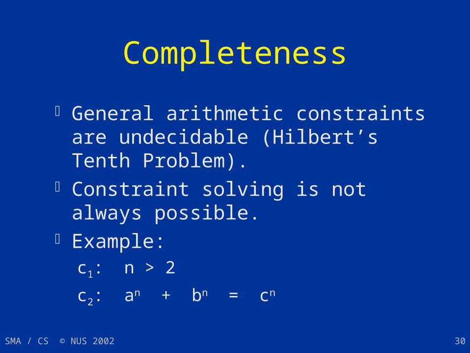
Completeness
General arithmetic constraints are undecidable (Hilbert’s Tenth Problem).
Constraint solving is not always possible. Example:
c1: n > 2
c2: an + bn = cn

SMA / CS © NUS 2002 31
The Constraint Programming Approach
Constraint programming separates constraints into
Basic constraints: constraint solving (complete) Non-basic constraints: propagation
(incomplete)
SMA / CS © NUS 2002 32
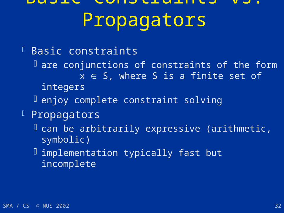
Basic Constraints vs. Propagators
Basic constraints are conjunctions of constraints of the form x S, where S is a finite set of integers
enjoy complete constraint solving Propagators
can be arbitrarily expressive (arithmetic, symbolic) implementation typically fast but incomplete
SMA / CS © NUS 2002 33
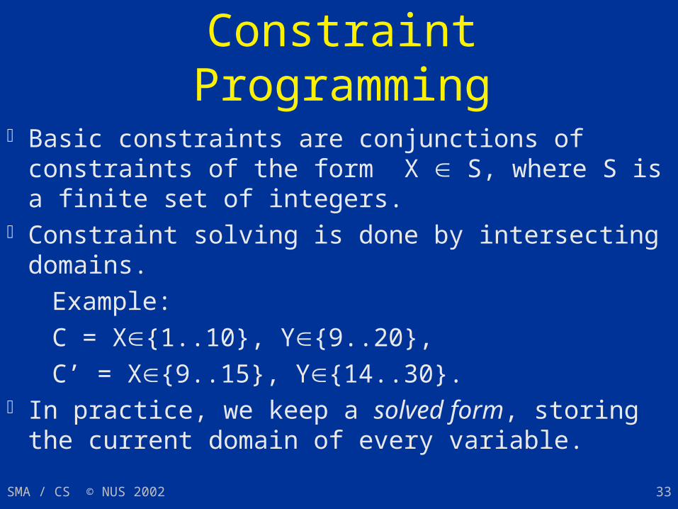
Basic Constraints in Constraint Programming
Basic constraints are conjunctions of constraints of the form X S, where S is a finite set of integers.
Constraint solving is done by intersecting domains.
Example:
C = X{1..10}, Y{9..20}, C’ = X{9..15}, Y{14..30}. In practice, we keep a solved form, storing the
current domain of every variable.
SMA / CS © NUS 2002 34
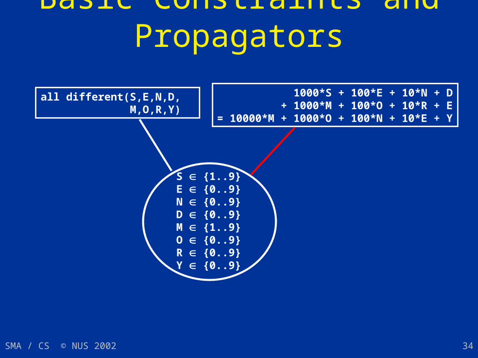
Basic Constraints and Propagators
S {1..9}E {0..9}N {0..9}D {0..9}M {1..9}O {0..9}R {0..9}Y {0..9}
all different(S,E,N,D, M,O,R,Y)
1000*S + 100*E + 10*N + D + 1000*M + 100*O + 10*R + E= 10000*M + 1000*O + 100*N + 10*E + Y
SMA / CS © NUS 2002 35
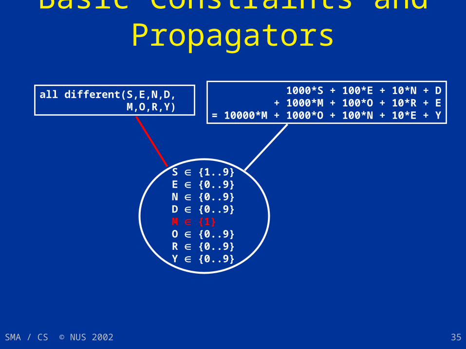
Basic Constraints and Propagators
S {1..9}E {0..9}N {0..9}D {0..9}M {1}O {0..9}R {0..9}Y {0..9}
all different(S,E,N,D, M,O,R,Y)
1000*S + 100*E + 10*N + D + 1000*M + 100*O + 10*R + E= 10000*M + 1000*O + 100*N + 10*E + Y
SMA / CS © NUS 2002 36
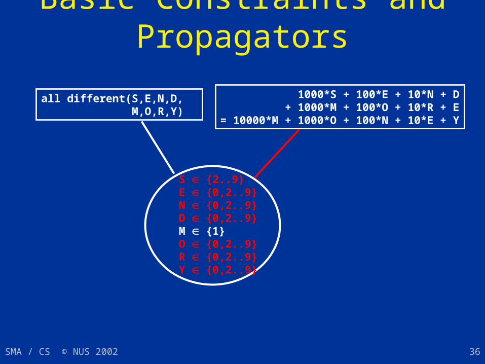
Basic Constraints and Propagators
S {2..9}E {0,2..9}N {0,2..9}D {0,2..9}M {1}O {0,2..9}R {0,2..9}Y {0,2..9}
all different(S,E,N,D, M,O,R,Y)
1000*S + 100*E + 10*N + D + 1000*M + 100*O + 10*R + E= 10000*M + 1000*O + 100*N + 10*E + Y
SMA / CS © NUS 2002 37
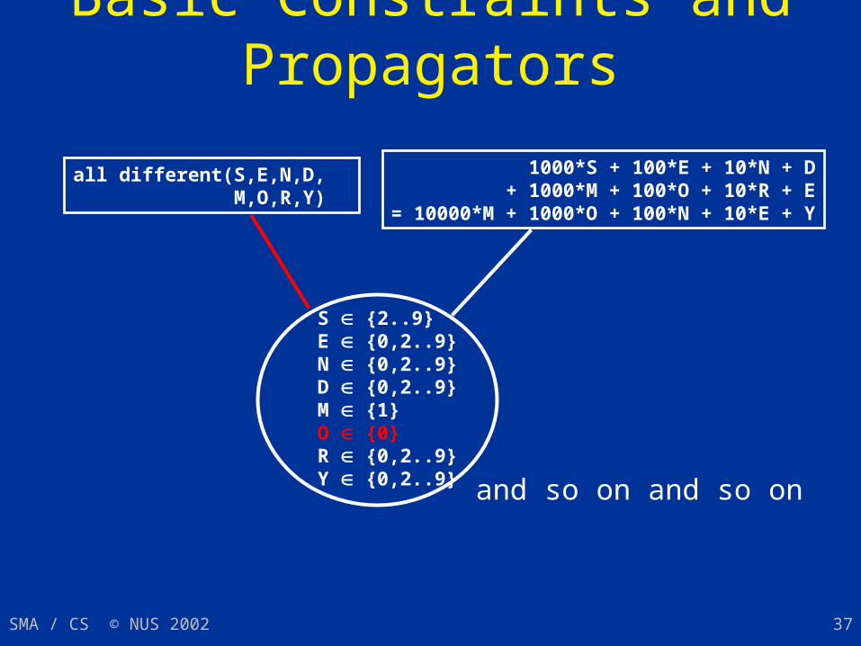
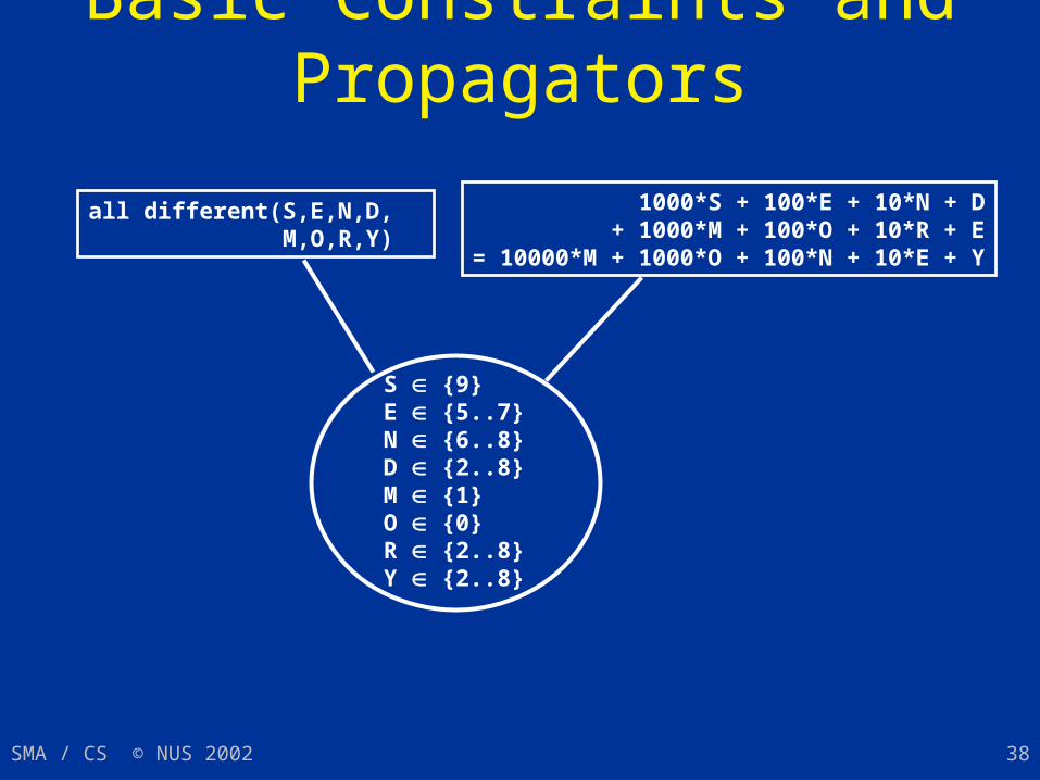
Basic Constraints and Propagators
S {2..9}E {0,2..9}N {0,2..9}D {0,2..9}M {1}O {0}R {0,2..9}Y {0,2..9}
all different(S,E,N,D, M,O,R,Y)
1000*S + 100*E + 10*N + D + 1000*M + 100*O + 10*R + E= 10000*M + 1000*O + 100*N + 10*E + Y
and so on and so on
SMA / CS © NUS 2002 38
Basic Constraints and Propagators
S {9}E {5..7}N {6..8}D {2..8}M {1}O {0}R {2..8}Y {2..8}
all different(S,E,N,D, M,O,R,Y)
1000*S + 100*E + 10*N + D + 1000*M + 100*O + 10*R + E= 10000*M + 1000*O + 100*N + 10*E + Y
SMA / CS © NUS 2002 39
Elements of Constraint Programming
The Approach Propagation Branching Exploration
SMA / CS © NUS 2002 40
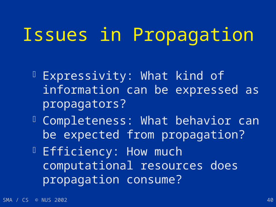
Issues in Propagation
Expressivity: What kind of information can be expressed as propagators?
Completeness: What behavior can be expected from propagation?
Efficiency: How much computational resources does propagation consume?
SMA / CS © NUS 2002 41
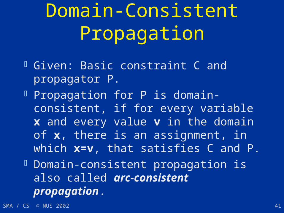
Domain-Consistent Propagation
Given: Basic constraint C and propagator P. Propagation for P is domain-consistent, if
for every variable x and every value v in the domain of x, there is an assignment, in which x=v, that satisfies C and P.
Domain-consistent propagation is also called arc-consistent propagation.
SMA / CS © NUS 2002 42
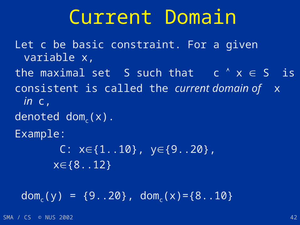
Current DomainLet c be basic constraint. For a given variable x,
the maximal set S such that c x S is
consistent is called the current domain of x in c,
denoted domc(x).
Example:
C: x{1..10}, y{9..20}, x{8..12}
domc(y) = {9..20}, domc(x)={8..10}
SMA / CS © NUS 2002 43
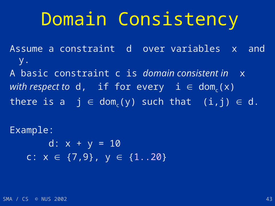
Domain Consistency
Assume a constraint d over variables x and y.
A basic constraint c is domain consistent in x
with respect to d, if for every i domc(x)
there is a j domc(y) such that (i,j) d.
Example:
d: x + y = 10
c: x {7,9}, y {1..20}
SMA / CS © NUS 2002 44
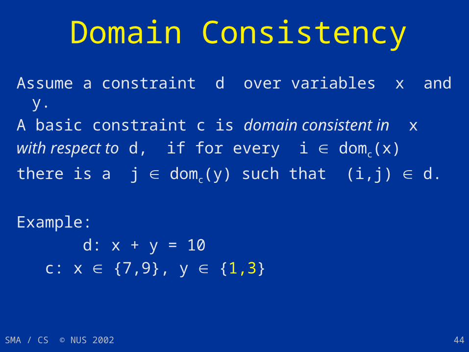
Domain Consistency
Assume a constraint d over variables x and y.
A basic constraint c is domain consistent in x
with respect to d, if for every i domc(x)
there is a j domc(y) such that (i,j) d.
Example:
d: x + y = 10
c: x {7,9}, y {1,3}
SMA / CS © NUS 2002 45
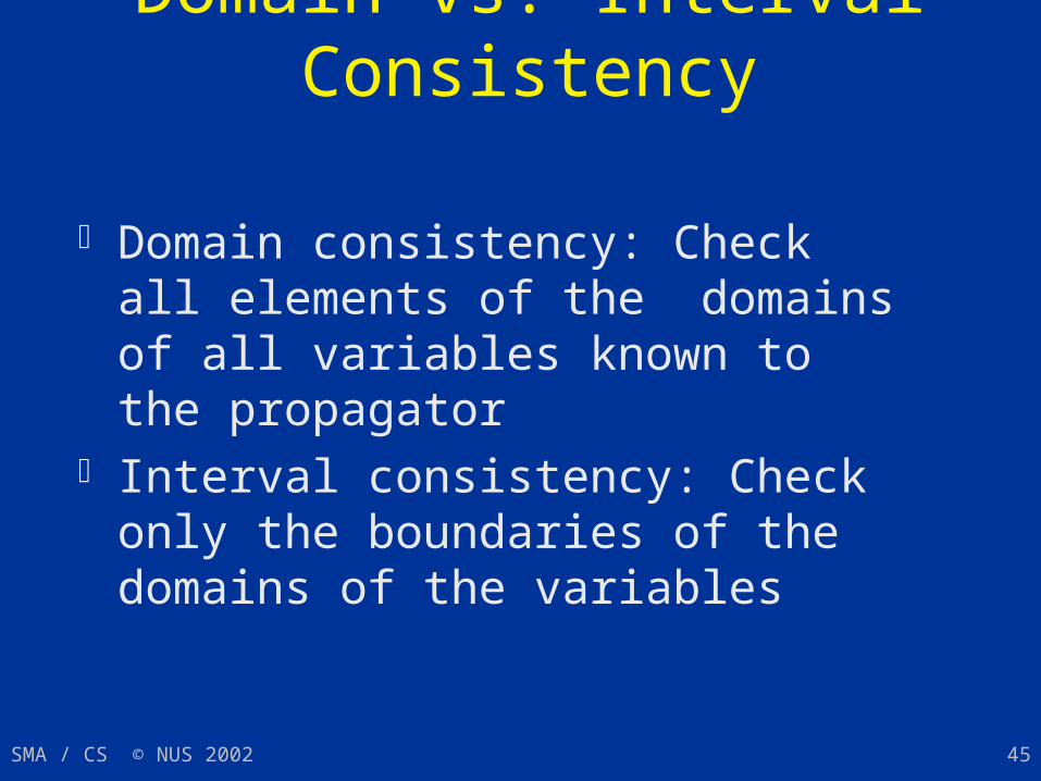
Domain vs. Interval Consistency
Domain consistency: Check all elements of the domains of all variables known to the propagator
Interval consistency: Check only the boundaries of the domains of the variables
SMA / CS © NUS 2002 46
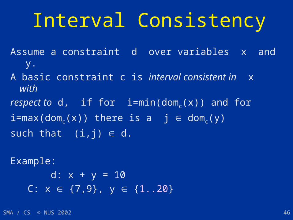
Interval Consistency
Assume a constraint d over variables x and y.
A basic constraint c is interval consistent in x with
respect to d, if for i=min(domc(x)) and for
i=max(domc(x)) there is a j domc(y)
such that (i,j) d.
Example:
d: x + y = 10
C: x {7,9}, y {1..20}
SMA / CS © NUS 2002 47
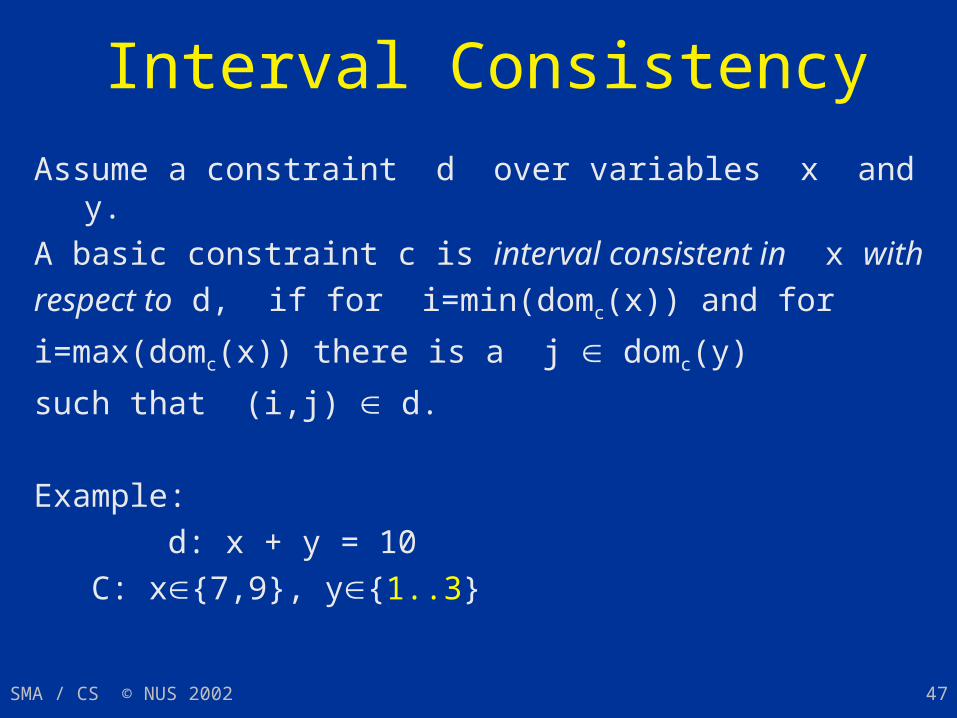
Interval Consistency
Assume a constraint d over variables x and y.
A basic constraint c is interval consistent in x with
respect to d, if for i=min(domc(x)) and for
i=max(domc(x)) there is a j domc(y)
such that (i,j) d.
Example:
d: x + y = 10
C: x{7,9}, y{1..3}
SMA / CS © NUS 2002 48
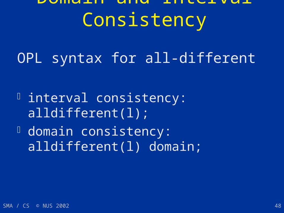
Domain and Interval Consistency
OPL syntax for all-different
interval consistency: alldifferent(l);
domain consistency: alldifferent(l) domain;
SMA / CS © NUS 2002 49
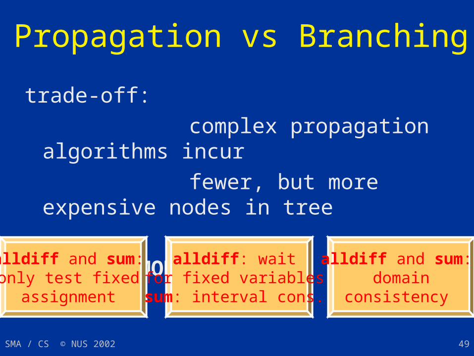
Propagation vs Branching
trade-off:
complex propagation algorithms incur
fewer, but more expensive nodes in tree
Example: MONEY with
alldiff and sum: only test fixed
assignment
alldiff: wait for fixed variables sum: interval cons.
alldiff and sum: domain
consistency
SMA / CS © NUS 2002 50
Elements of Constraint Programming
The Approach Propagation Branching Exploration
SMA / CS © NUS 2002 51
Branching Algorithms
Constraint programming systems come with libraries of predefined branching algorithms programming support for user-defined
branching algorithms
SMA / CS © NUS 2002 52
Branching for MONEY enum Letter {S,E,N,D,M,O,R,Y};var int l[Letter] in 0..9;solve { alldifferent(l); l[S] <> 0; l[M] <> 0; l[S]*1000 + l[E]*100 + l[N]*10 + l[D] + l[M]*1000 + l[O]*100 + l[R]*10 + l[E] = l[M]*10000 + l[O]*1000 + l[N]*100 + l[E]*10 + l[Y] };search { forall(i in Letter ordered by increasing dsize(l[i])) tryall(v in 0..9) l[i] = v; };All Solutions; Execution Run
SMA / CS © NUS 2002 53
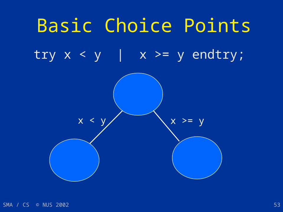
Basic Choice Points
try x < y | x >= y endtry;
x < y x >= y
SMA / CS © NUS 2002 54
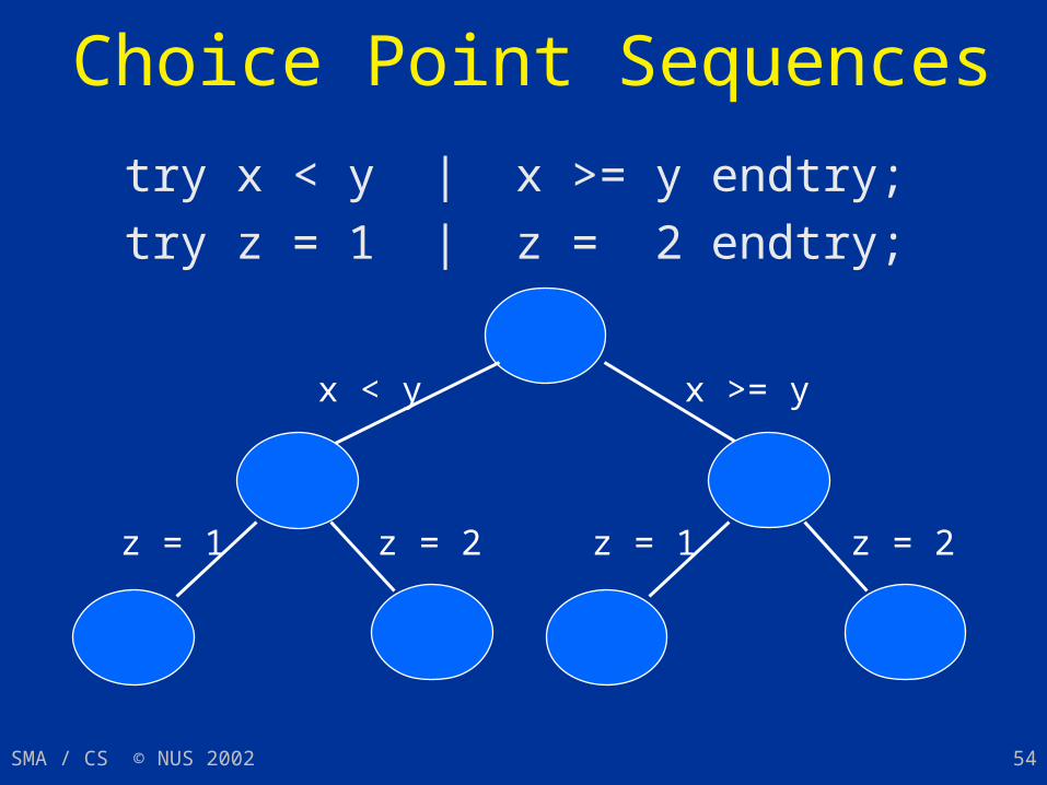
Choice Point Sequences
try x < y | x >= y endtry;
try z = 1 | z = 2 endtry;
x < y x >= y
z = 1 z = 2 z = 1 z = 2

SMA / CS © NUS 2002 55
Abbreviation: tryall
tryall(i in 1..5) x = i;
stands for
try x=1|x=2|x=3|x=4|x=5 endtry;
SMA / CS © NUS 2002 56
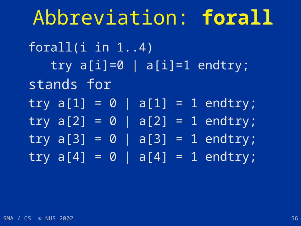
Abbreviation: forallforall(i in 1..4)
try a[i]=0 | a[i]=1 endtry;
stands fortry a[1] = 0 | a[1] = 1 endtry;
try a[2] = 0 | a[2] = 1 endtry;
try a[3] = 0 | a[3] = 1 endtry;
try a[4] = 0 | a[4] = 1 endtry;
SMA / CS © NUS 2002 57
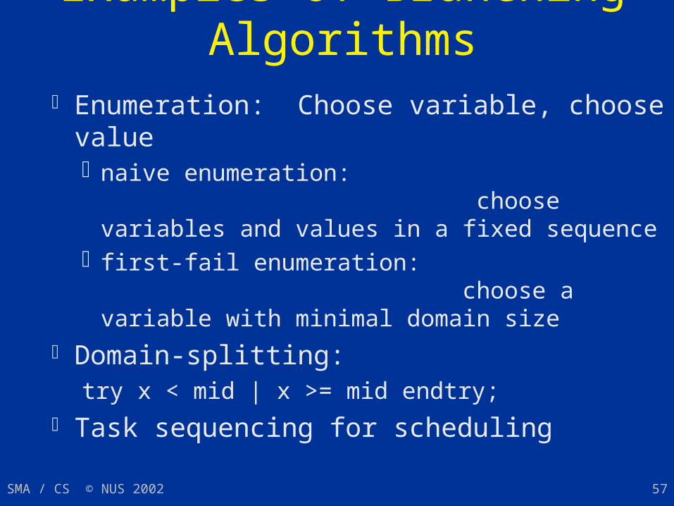
Examples of Branching Algorithms Enumeration: Choose variable, choose value
naive enumeration: choose variables and values in a fixed sequence
first-fail enumeration: choose a variable with minimal domain size
Domain-splitting:try x < mid | x >= mid endtry;
Task sequencing for scheduling
SMA / CS © NUS 2002 58
Elements of Constraint Programming
The Approach Propagation Branching Exploration
SMA / CS © NUS 2002 59
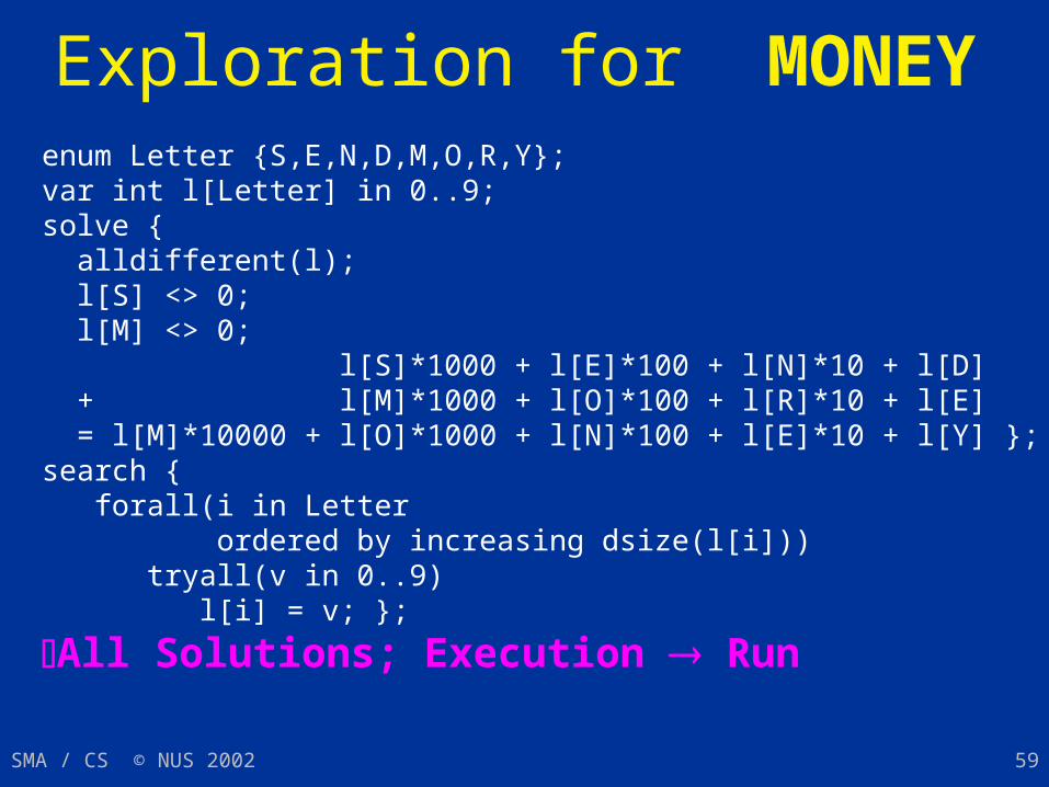
Exploration for MONEY enum Letter {S,E,N,D,M,O,R,Y};var int l[Letter] in 0..9;solve { alldifferent(l); l[S] <> 0; l[M] <> 0; l[S]*1000 + l[E]*100 + l[N]*10 + l[D] + l[M]*1000 + l[O]*100 + l[R]*10 + l[E] = l[M]*10000 + l[O]*1000 + l[N]*100 + l[E]*10 + l[Y] };search { forall(i in Letter ordered by increasing dsize(l[i])) tryall(v in 0..9) l[i] = v; };
All Solutions; Execution Run
SMA / CS © NUS 2002 60
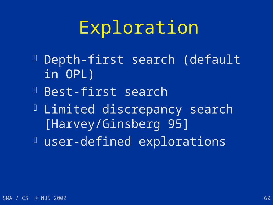
Exploration
Depth-first search (default in OPL) Best-first search Limited discrepancy search
[Harvey/Ginsberg 95] user-defined explorations
SMA / CS © NUS 2002 61
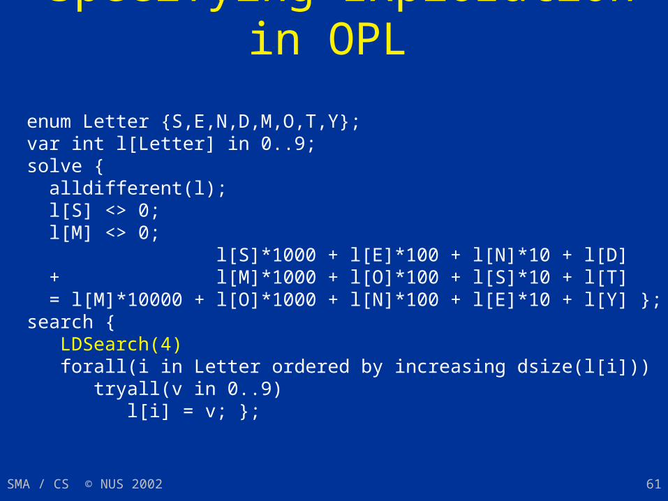
Specifying Exploration in OPL
enum Letter {S,E,N,D,M,O,T,Y};var int l[Letter] in 0..9;solve { alldifferent(l); l[S] <> 0; l[M] <> 0; l[S]*1000 + l[E]*100 + l[N]*10 + l[D] + l[M]*1000 + l[O]*100 + l[S]*10 + l[T] = l[M]*10000 + l[O]*1000 + l[N]*100 + l[E]*10 + l[Y] };search { LDSearch(4) forall(i in Letter ordered by increasing dsize(l[i])) tryall(v in 0..9) l[i] = v; };
SMA / CS © NUS 2002 62
Other Search Components
Optimization Interaction Visualization
SMA / CS © NUS 2002 63
Optimization
SEND + MOST = MONEY

SMA / CS © NUS 2002 64
Optimization in OPL
enum Letter {S,E,N,D,M,O,T,Y};var int l[Letter] in 0..9;maximize money subject to { money = l[M]*10000+l[O]*1000+l[N]*100+l[E]*10+l[Y] alldifferent(l); l[S] <> 0; l[M] <> 0; l[S]*1000 + l[E]*100 + l[N]*10 + l[D] + l[M]*1000 + l[O]*100 + l[S]*10 + l[T] = l[M]*10000 + l[O]*1000 + l[N]*100 + l[E]*10 + l[Y] };search { forall(i in Letter ordered by increasing dsize(l[i])) tryall(v in 0..9) l[i] = v; };
All Solutions; Execution Run
SMA / CS © NUS 2002 65
Interaction
First-solution search All solution search Last solution search Search with user interaction
SMA / CS © NUS 2002 66
Visualization
Example: Oz Explorer [Schulte 1997].
Oz Explorer combines visualization first/all solution / user interaction branch-and-bound optimization depth-first search

SMA / CS © NUS 2002 67
Overview
Constraint programming in a nutshell Elements of constraint programming Sport tournament scheduling Production scheduling Assessment

SMA / CS © NUS 2002 68
Sport Tournament Scheduling
CP Approach Propagators Example

SMA / CS © NUS 2002 69
Sport Tournament Scheduling
CP Approach Propagators Example
SMA / CS © NUS 2002 70
Round Robin Tournament Planning Problems
n teams, each playing a fixed number of times r against every other team
r = 1: single, r = 2: double round robin. Each match is home match for one and
away match for the other Dense round robin:
At each date, each team plays at most once. The number of dates is minimal.
SMA / CS © NUS 2002 71
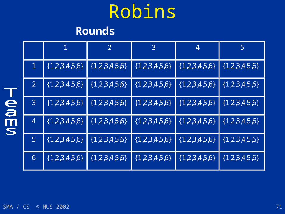
CP Approach to Round Robins
1 2 3 4 5
1 {1,2,3,4,5,6} {1,2,3,4,5,6} {1,2,3,4,5,6} {1,2,3,4,5,6} {1,2,3,4,5,6}
2 {1,2,3,4,5,6} {1,2,3,4,5,6} {1,2,3,4,5,6} {1,2,3,4,5,6} {1,2,3,4,5,6}
3 {1,2,3,4,5,6} {1,2,3,4,5,6} {1,2,3,4,5,6} {1,2,3,4,5,6} {1,2,3,4,5,6}
4 {1,2,3,4,5,6} {1,2,3,4,5,6} {1,2,3,4,5,6} {1,2,3,4,5,6} {1,2,3,4,5,6}
5 {1,2,3,4,5,6} {1,2,3,4,5,6} {1,2,3,4,5,6} {1,2,3,4,5,6} {1,2,3,4,5,6}
6 {1,2,3,4,5,6} {1,2,3,4,5,6} {1,2,3,4,5,6} {1,2,3,4,5,6} {1,2,3,4,5,6}
Rounds
SMA / CS © NUS 2002 72
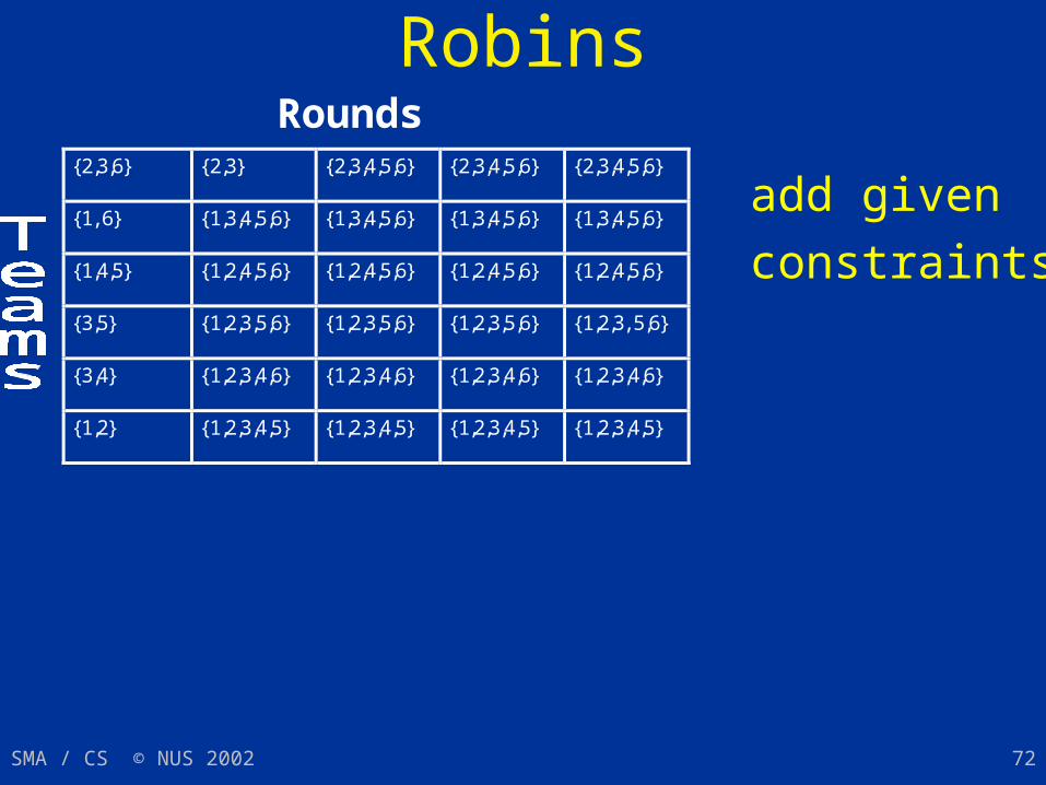
CP Approach to Round Robins
{2,3,6} {2,3} {2,3,4,5,6} {2,3,4,5,6} {2,3,4,5,6}
{1, 6} {1,3,4,5,6} {1,3,4,5,6} {1,3,4,5,6} {1,3,4,5,6}
{1,4,5} {1,2,4,5,6} {1,2,4,5,6} {1,2,4,5,6} {1,2,4,5,6}
{3,5} {1,2,3,5,6} {1,2,3,5,6} {1,2,3,5,6} {1,2,3, 5,6}
{3,4} {1,2,3,4,6} {1,2,3,4,6} {1,2,3,4,6} {1,2,3,4,6}
{1,2} {1,2,3,4,5} {1,2,3,4,5} {1,2,3,4,5} {1,2,3,4,5}
add given
constraints
Rounds
SMA / CS © NUS 2002 73
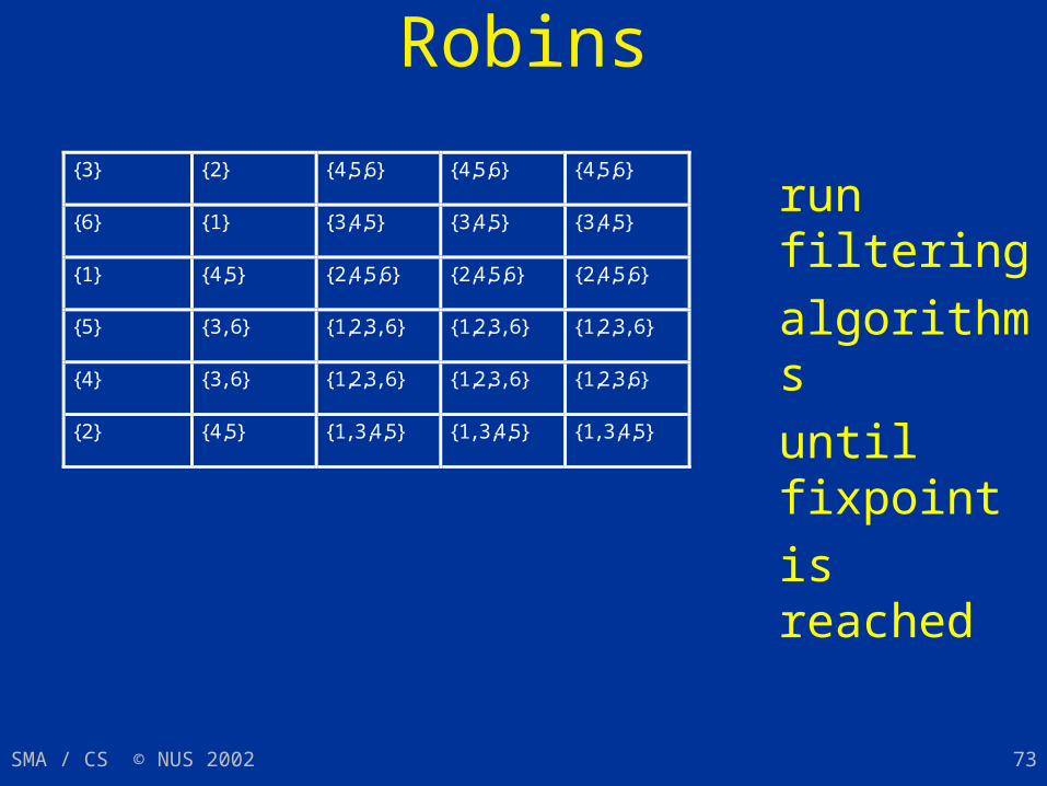
CP Approach to Round Robins
{3} {2} {4,5,6} {4,5,6} {4,5,6}
{6} {1} {3,4,5} {3,4,5} {3,4,5}
{1} {4,5} {2,4,5,6} {2,4,5,6} {2,4,5,6}
{5} {3, 6} {1,2,3, 6} {1,2,3, 6} {1,2,3, 6}
{4} {3, 6} {1,2,3, 6} {1,2,3, 6} {1,2,3,6}
{2} {4,5} {1, 3,4,5} {1, 3,4,5} {1, 3,4,5}
run filtering
algorithms
until fixpoint
is reached
SMA / CS © NUS 2002 74
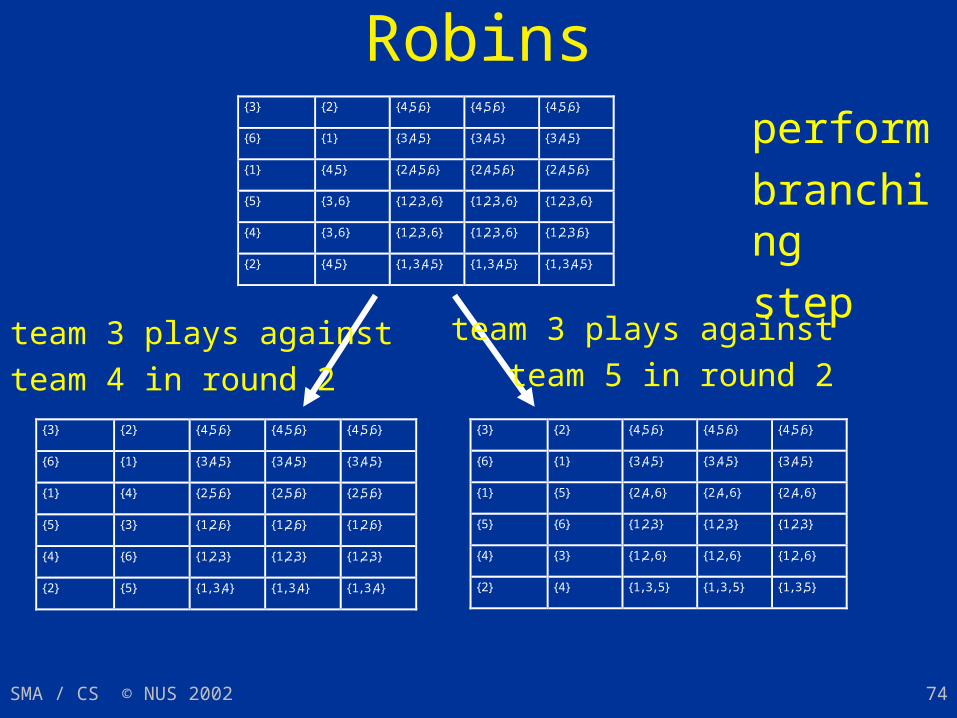
CP Approach to Round Robins{3} {2} {4,5,6} {4,5,6} {4,5,6}
{6} {1} {3,4,5} {3,4,5} {3,4,5}
{1} {4,5} {2,4,5,6} {2,4,5,6} {2,4,5,6}
{5} {3, 6} {1,2,3, 6} {1,2,3, 6} {1,2,3, 6}
{4} {3, 6} {1,2,3, 6} {1,2,3, 6} {1,2,3,6}
{2} {4,5} {1, 3,4,5} {1, 3,4,5} {1, 3,4,5}
perform
branching
step
team 3 plays against
team 4 in round 2
team 3 plays against
team 5 in round 2
{3} {2} {4,5,6} {4,5,6} {4,5,6}
{6} {1} {3,4,5} {3,4,5} {3,4,5}
{1} {5} {2,4, 6} {2,4, 6} {2,4, 6}
{5} {6} {1,2,3} {1,2,3} {1,2,3}
{4} {3} {1,2, 6} {1,2, 6} {1,2, 6}
{2} {4} {1, 3, 5} {1, 3, 5} {1, 3,5}
{3} {2} {4,5,6} {4,5,6} {4,5,6}
{6} {1} {3,4,5} {3,4,5} {3,4,5}
{1} {4} {2,5,6} {2,5,6} {2,5,6}
{5} {3} {1,2,6} {1,2,6} {1,2,6}
{4} {6} {1,2,3} {1,2,3} {1,2,3}
{2} {5} {1, 3,4} {1, 3,4} {1, 3,4}
SMA / CS © NUS 2002 75
Sport Tournament Scheduling
CP Approach Propagators Example
SMA / CS © NUS 2002 76
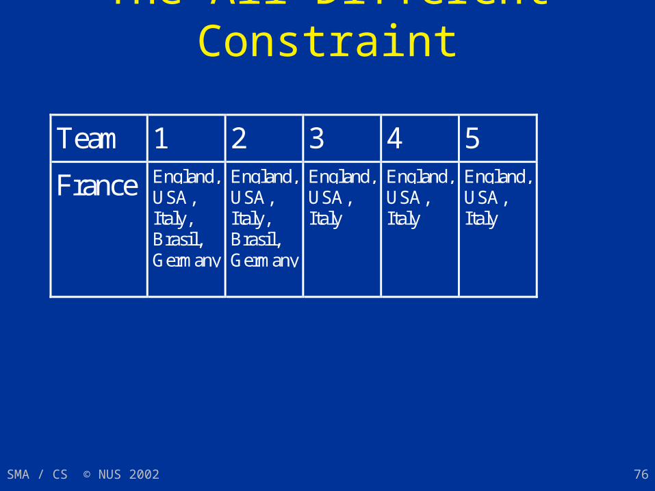
The All-Different Constraint
Team 1 2 3 4 5
France England,USA,Italy,Brasil,Germany
England,USA,Italy,Brasil,Germany
England,USA,Italy
England,USA,Italy
England,USA,Italy

SMA / CS © NUS 2002 77
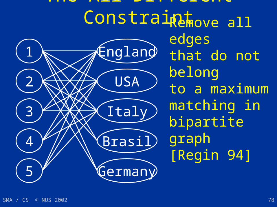
The All-Different Constraint
1
5
4
2
3
England
Germany
Brasil
USA
Italy
SMA / CS © NUS 2002 78
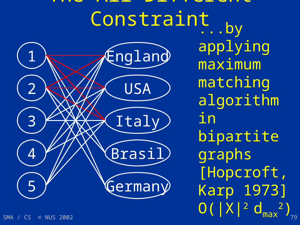
The All-Different Constraint
1
5
4
2
3
England
Germany
Brasil
USA
Italy
Remove all edgesthat do not belongto a maximum matching in bipartite graph[Regin 94]
SMA / CS © NUS 2002 79
The All-Different Constraint
1
5
4
2
3
England
Germany
Brasil
USA
Italy
...by applyingmaximum matching algorithm in bipartite graphs[Hopcroft, Karp 1973] O(|X|2 dmax
2)
SMA / CS © NUS 2002 80
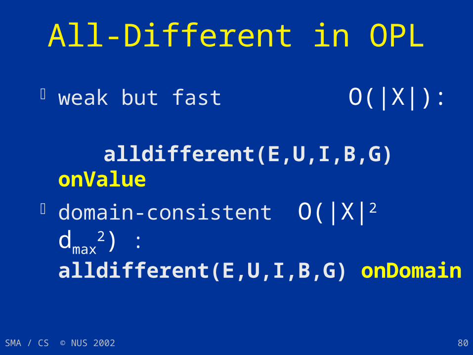
All-Different in OPL
weak but fast O(|X|): alldifferent(E,U,I,B,G) onValue domain-consistent O(|X|2 dmax
2) : alldifferent(E,U,I,B,G) onDomain
SMA / CS © NUS 2002 81
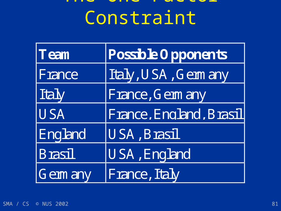
The One-Factor Constraint
Team Possible Opponents
France Italy, USA, Germany
Italy France, Germany
USA France, England, Brasil
England USA, Brasil
Brasil USA, England
Germany France, Italy

SMA / CS © NUS 2002 82
The One-Factor Constraint
France
Italy USA
England
Germany
Brasil
SMA / CS © NUS 2002 83
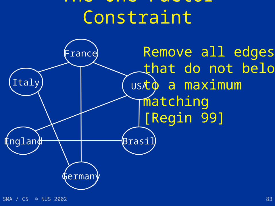
The One-Factor Constraint
France
Italy USA
England
Germany
Brasil
Remove all edgesthat do not belongto a maximum matching[Regin 99]
SMA / CS © NUS 2002 84
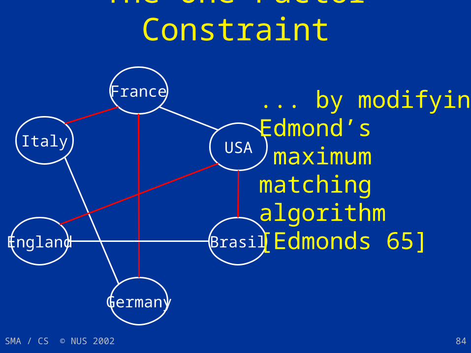
The One-Factor Constraint
France
Italy USA
England
Germany
Brasil
... by modifyingEdmond’s maximum matching algorithm[Edmonds 65]
SMA / CS © NUS 2002 85
Sport Tournament Scheduling
CP Approach Propagators Example
SMA / CS © NUS 2002 86
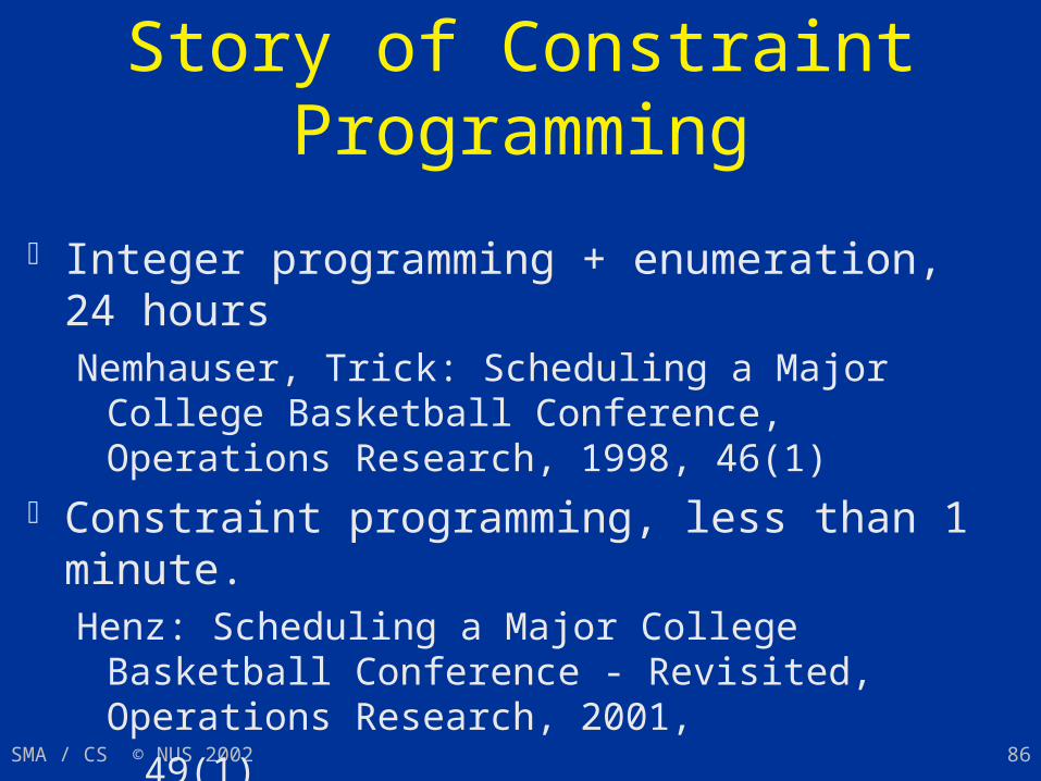
ACC 1997/98: A Success Story of Constraint Programming
Integer programming + enumeration, 24 hoursNemhauser, Trick: Scheduling a Major College
Basketball Conference, Operations Research, 1998, 46(1)
Constraint programming, less than 1 minute.Henz: Scheduling a Major College Basketball
Conference - Revisited, Operations Research, 2001,
49(1)

SMA / CS © NUS 2002 87
The ACC 1997/98 Problem
9 teams participate in tournament Dense double round robin:
there are 2 * 9 dates at each date, each team plays either home, away
or has a “bye” Alternating weekday and weekend matches
SMA / CS © NUS 2002 88
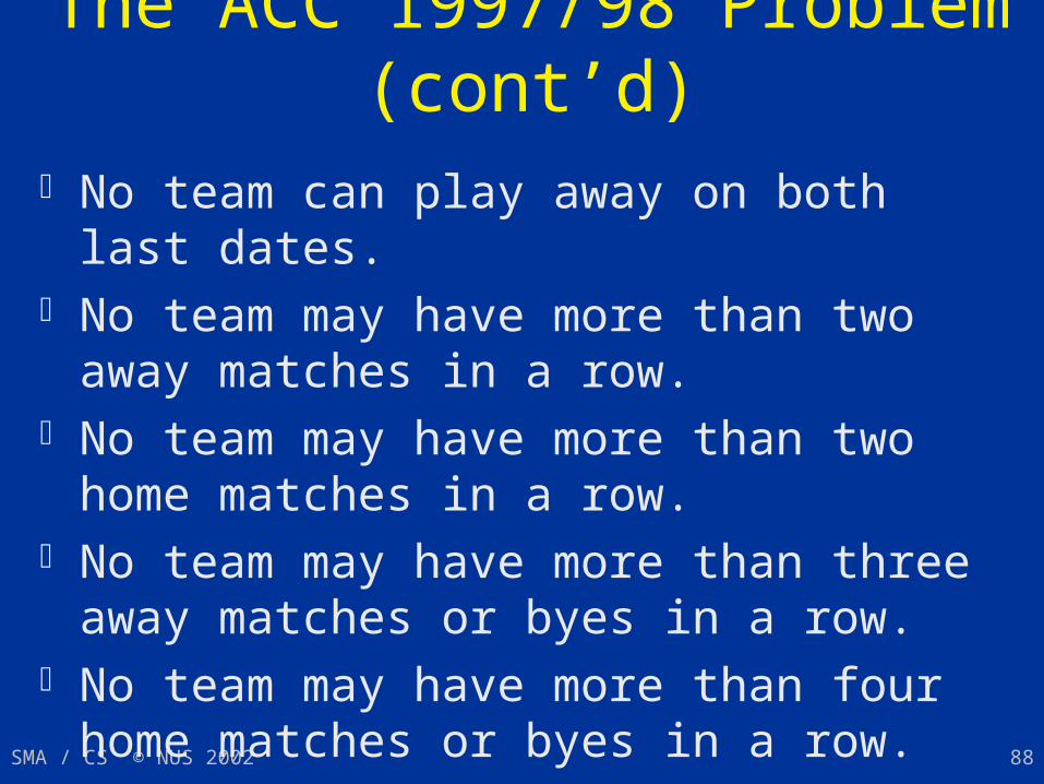
The ACC 1997/98 Problem (cont’d) No team can play away on both last dates. No team may have more than two away matches
in a row. No team may have more than two home matches
in a row. No team may have more than three away
matches or byes in a row. No team may have more than four home matches
or byes in a row.
SMA / CS © NUS 2002 89
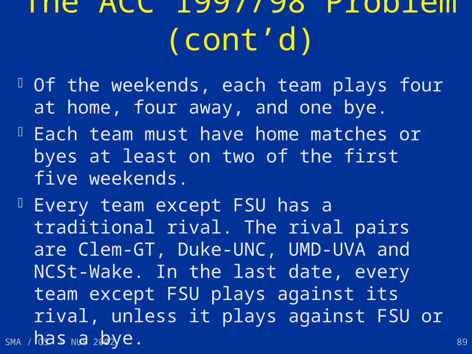
The ACC 1997/98 Problem (cont’d) Of the weekends, each team plays four at home,
four away, and one bye. Each team must have home matches or byes at
least on two of the first five weekends. Every team except FSU has a traditional rival.
The rival pairs are Clem-GT, Duke-UNC, UMD-UVA and NCSt-Wake. In the last date, every team except FSU plays against its rival, unless it plays against FSU or has a bye.
SMA / CS © NUS 2002 90
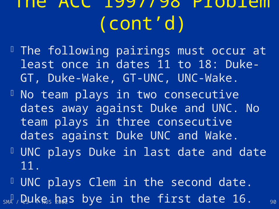
The ACC 1997/98 Problem (cont’d) The following pairings must occur at least once
in dates 11 to 18: Duke-GT, Duke-Wake, GT-UNC, UNC-Wake.
No team plays in two consecutive dates away against Duke and UNC. No team plays in three consecutive dates against Duke UNC and Wake.
UNC plays Duke in last date and date 11. UNC plays Clem in the second date. Duke has bye in the first date 16.
SMA / CS © NUS 2002 91
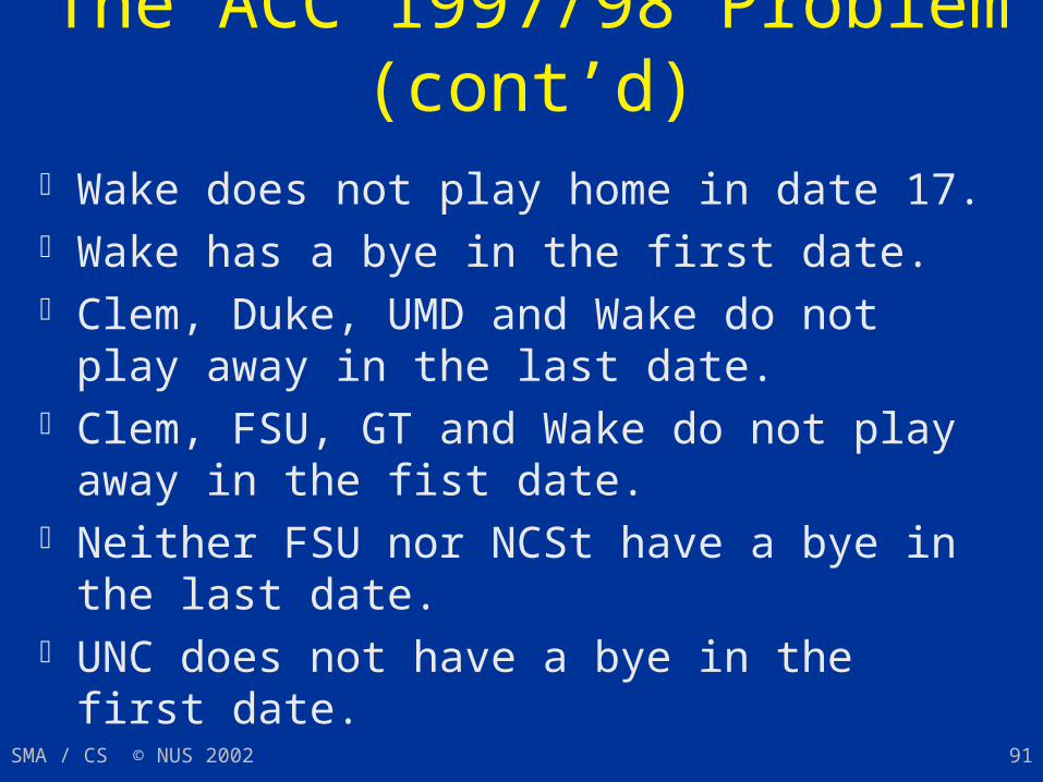
The ACC 1997/98 Problem (cont’d) Wake does not play home in date 17. Wake has a bye in the first date. Clem, Duke, UMD and Wake do not play away
in the last date. Clem, FSU, GT and Wake do not play away in
the fist date. Neither FSU nor NCSt have a bye in the last
date. UNC does not have a bye in the first date.
SMA / CS © NUS 2002 92
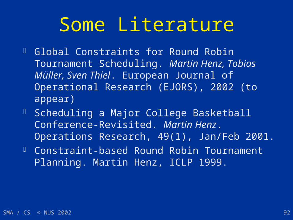
Some Literature Global Constraints for Round Robin Tournament
Scheduling. Martin Henz, Tobias Müller, Sven Thiel. European Journal of Operational Research (EJORS), 2002 (to appear)
Scheduling a Major College Basketball Conference-Revisited. Martin Henz. Operations Research, 49(1), Jan/Feb 2001.
Constraint-based Round Robin Tournament Planning. Martin Henz, ICLP 1999.
SMA / CS © NUS 2002 93
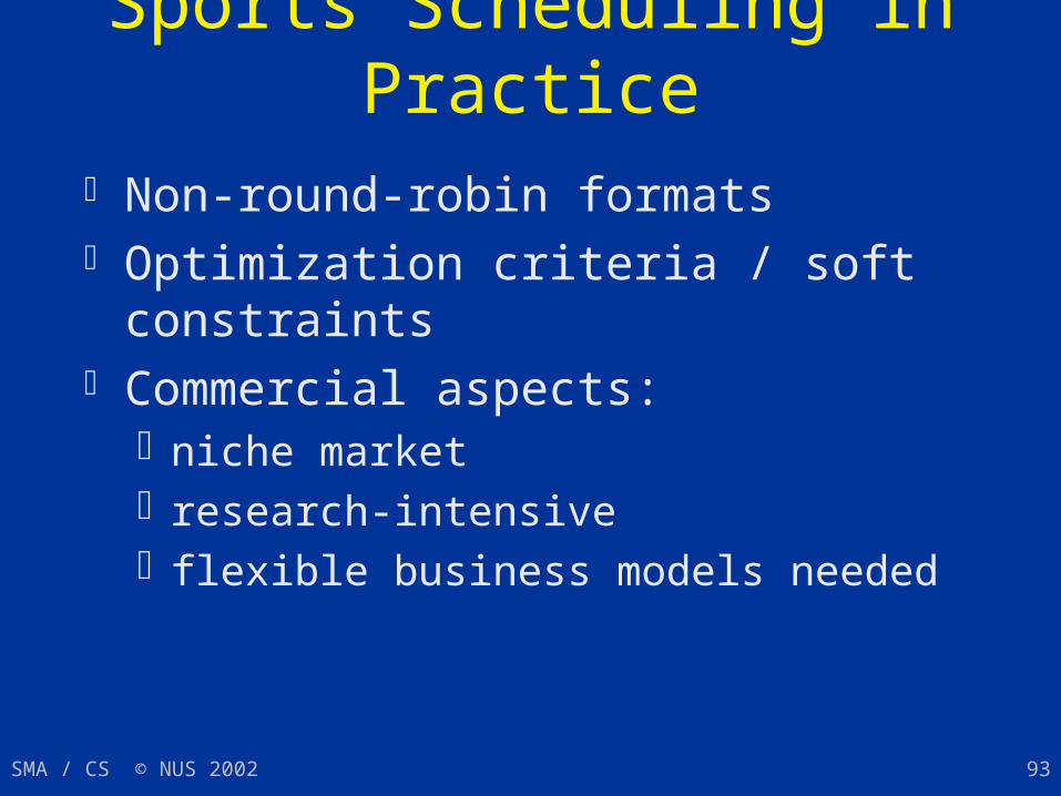
Sports Scheduling in Practice Non-round-robin formats Optimization criteria / soft constraints Commercial aspects:
niche market research-intensive flexible business models needed
SMA / CS © NUS 2002 94
Overview
Constraint programming in a nutshell Elements of constraint programming Sport tournament scheduling Production scheduling Assessment
SMA / CS © NUS 2002 95
Production Scheduling Problems
Scheduling Problems Propagation Algorithms for Resource
Constraints Branching Algorithms Exploration Algorithms Literature
SMA / CS © NUS 2002 96
Production Scheduling Problems
Scheduling Problems Propagation Algorithms for Resource
Constraints Branching Algorithms Exploration Algorithms Literature
SMA / CS © NUS 2002 97
Scheduling Problems
Assign starting times (and sometimes durations) to tasks, subject to
resource constraints, precedence constraints, and various other constraints, and
an optimization function, typically to minimize overall schedule duration.
SMA / CS © NUS 2002 98
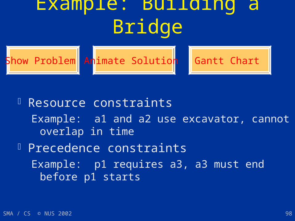
Example: Building a Bridge
Show Problem
Resource constraintsExample: a1 and a2 use excavator, cannot overlap in
time Precedence constraints
Example: p1 requires a3, a3 must end before p1 starts
Animate Solution Gantt Chart
SMA / CS © NUS 2002 99
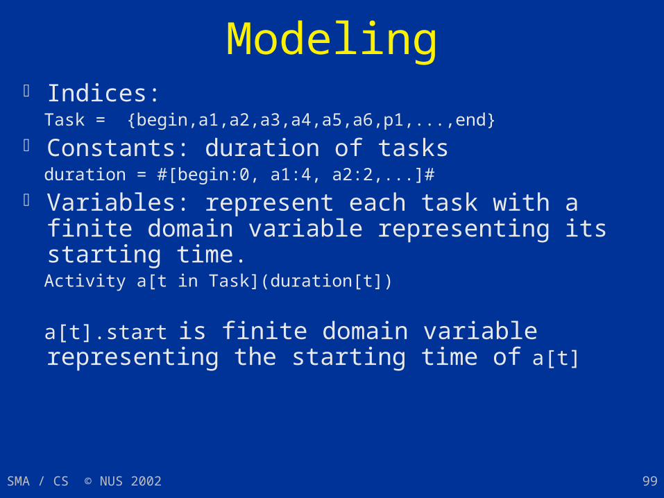
Modeling Indices: Task = {begin,a1,a2,a3,a4,a5,a6,p1,...,end}
Constants: duration of tasks duration = #[begin:0, a1:4, a2:2,...]#
Variables: represent each task with a finite domain variable representing its starting time.
Activity a[t in Task](duration[t])
a[t].start is finite domain variable representing the starting time of a[t]
SMA / CS © NUS 2002 100
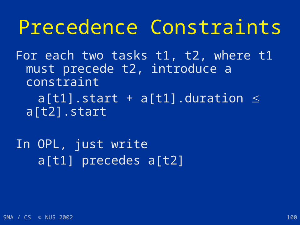
Precedence ConstraintsFor each two tasks t1, t2, where t1 must precede t2, introduce a constraint
a[t1].start + a[t1].duration a[t2].start
In OPL, just write a[t1] precedes a[t2]
SMA / CS © NUS 2002 101
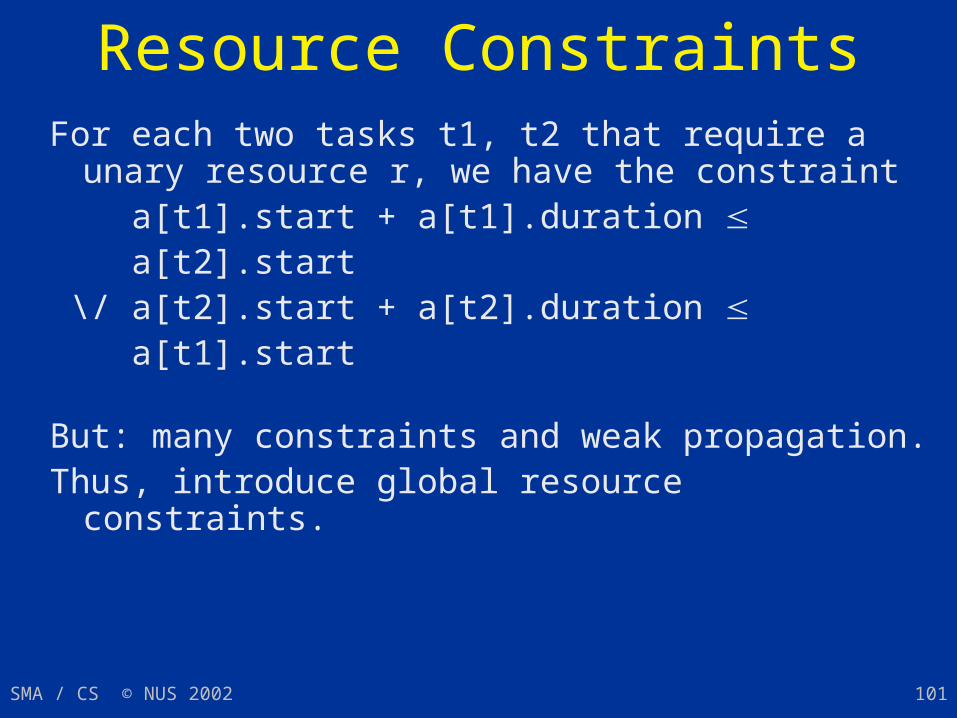
Resource ConstraintsFor each two tasks t1, t2 that require a unary resource r, we
have the constraint a[t1].start + a[t1].duration a[t2].start \/ a[t2].start + a[t2].duration a[t1].start
But: many constraints and weak propagation.Thus, introduce global resource constraints.
SMA / CS © NUS 2002 102
Scheduling
Scheduling Problems Propagation Algorithms for Resource
Constraints Branching Algorithms Literature
SMA / CS © NUS 2002 103
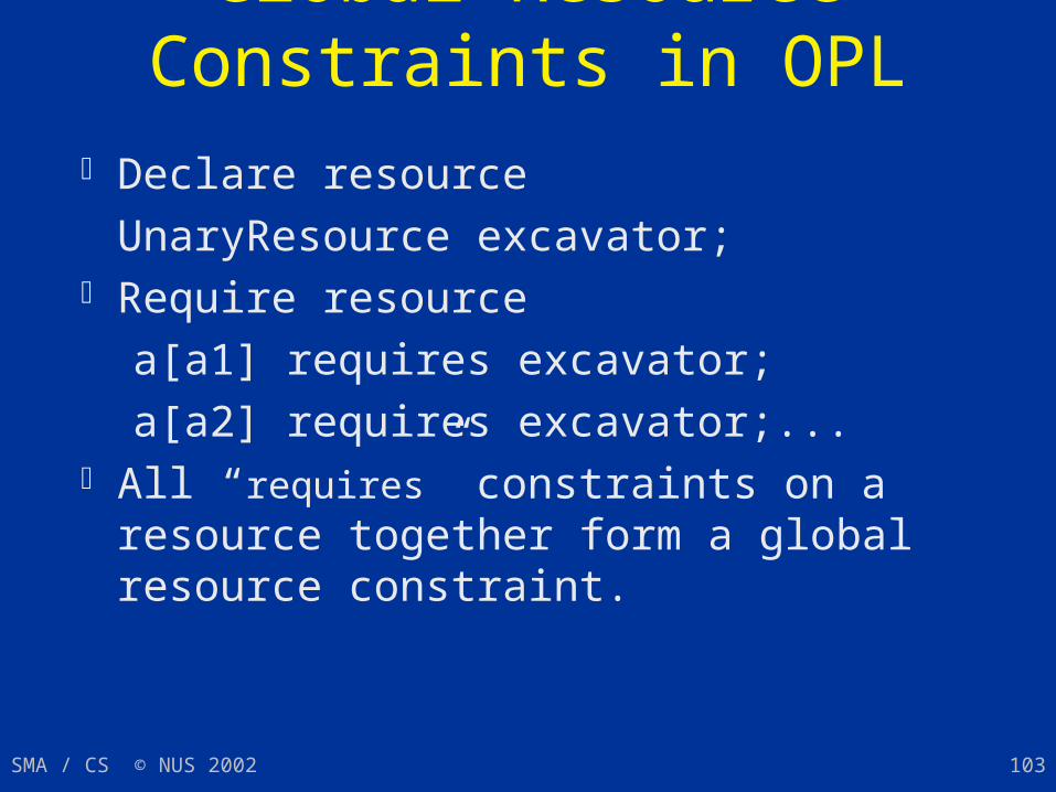
Global Resource Constraints in OPL Declare resource
UnaryResource excavator; Require resource
a[a1] requires excavator;
a[a2] requires excavator;... All “requires” constraints on a resource
together form a global resource constraint.
SMA / CS © NUS 2002 104
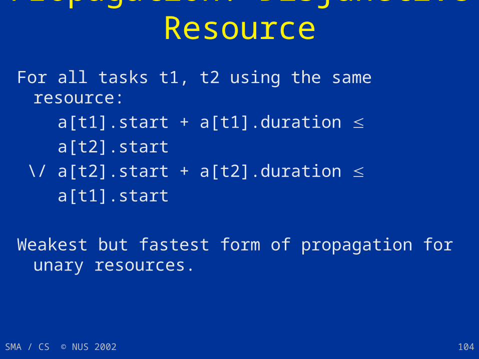
Propagation: Disjunctive Resource
For all tasks t1, t2 using the same resource:
a[t1].start + a[t1].duration
a[t2].start
\/ a[t2].start + a[t2].duration a[t1].start
Weakest but fastest form of propagation for unary resources.
SMA / CS © NUS 2002 105
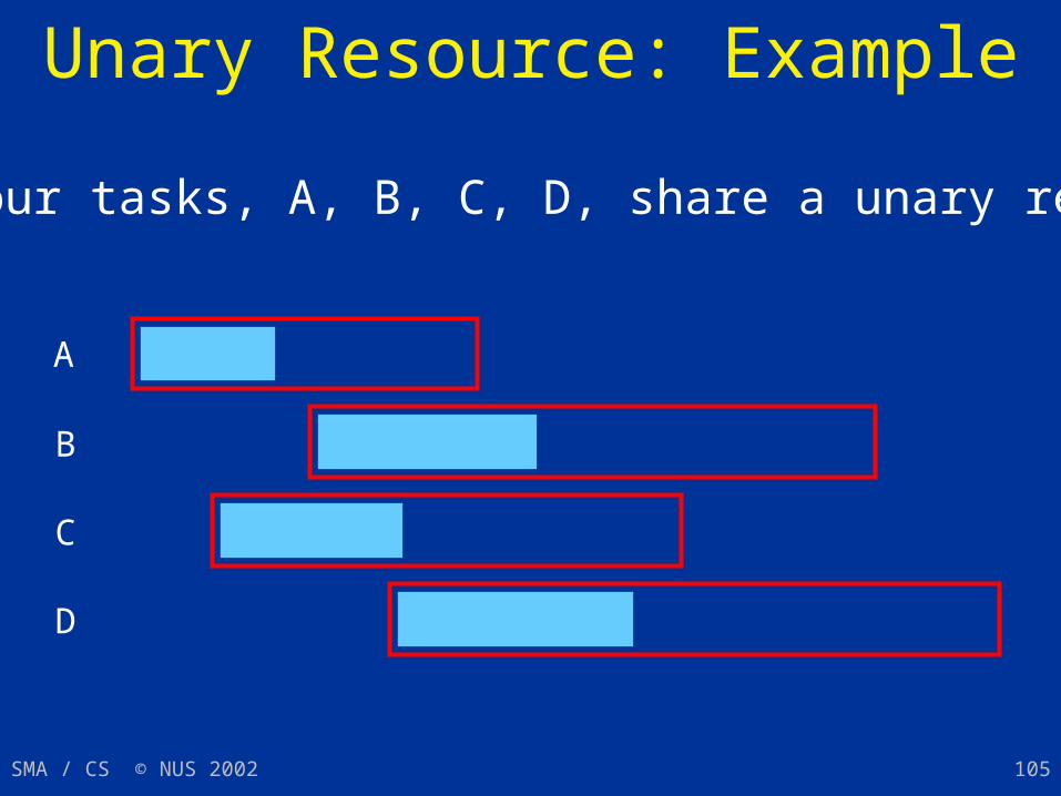
Unary Resource: Example
A
B
C
D
The four tasks, A, B, C, D, share a unary resource.
SMA / CS © NUS 2002 106
Propagation: Edge finding
For a given task t and set of tasks S, all sharing the same unary resource , find out whether t can occur
before all tasks in S, after all tasks in S, between two tasks in S,
and infer corresponding basic constraints.
SMA / CS © NUS 2002 107
Which Edge Finder?As usual, trade-off between run-time of propagation
algorithm and strength of propagation. Edge finding can be expensive depending on what tasks are considered.
Recent edge finders have complexity n2 for one propagation step, where n is the number of tasks using the resource.
Edge finding based on task intervals can be stronger than these, but typically have complexity n3 .
SMA / CS © NUS 2002 108
Specifying Propagation Algorithms
OPL fixes propagation for unary resources to an (undisclosed) edge-finding algorithm.
For discrete (non-unary) resources, the user can choose between default, disjunctive and edgeFinder when declaring a resource. Example:
DiscreteResource crane(3) using edgeFinder;

SMA / CS © NUS 2002 109
Demo: Propagation for Unary Resources
Bridge
SMA / CS © NUS 2002 110
Scheduling
Scheduling Problems Propagation Algorithms for Resource
Constraints Branching Algorithms Literature
SMA / CS © NUS 2002 111
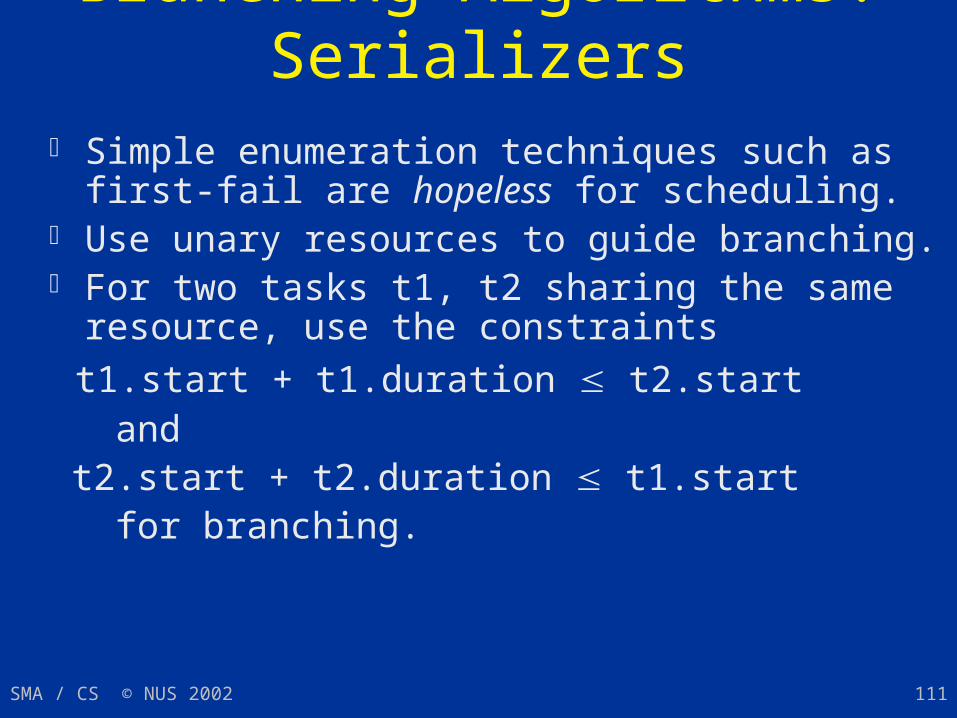
Branching Algorithms: Serializers Simple enumeration techniques such as first-fail are
hopeless for scheduling. Use unary resources to guide branching. For two tasks t1, t2 sharing the same resource, use the
constraints
t1.start + t1.duration t2.start and t2.start + t2.duration t1.start for branching.
SMA / CS © NUS 2002 112
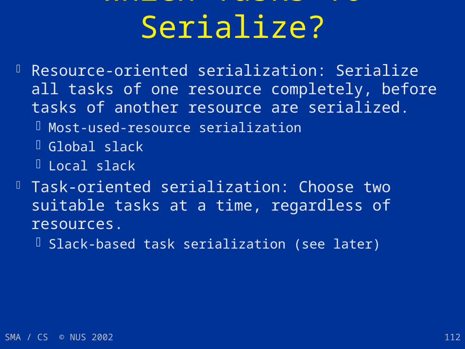
Which Tasks To Serialize? Resource-oriented serialization: Serialize all tasks of
one resource completely, before tasks of another resource are serialized. Most-used-resource serialization Global slack Local slack
Task-oriented serialization: Choose two suitable tasks at a time, regardless of resources. Slack-based task serialization (see later)
SMA / CS © NUS 2002 113
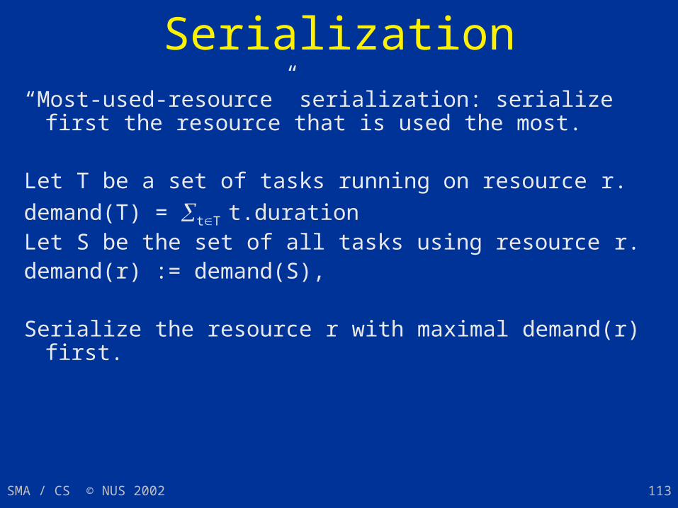
Most-used-resource Serialization“Most-used-resource” serialization: serialize first the
resource that is used the most.
Let T be a set of tasks running on resource r.
demand(T) = tT t.durationLet S be the set of all tasks using resource r.demand(r) := demand(S),
Serialize the resource r with maximal demand(r) first.
SMA / CS © NUS 2002 114
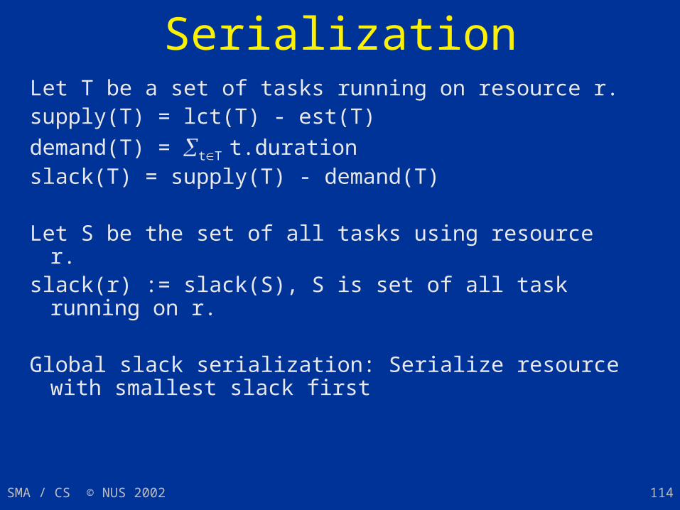
Slack-based Resource SerializationLet T be a set of tasks running on resource r.supply(T) = lct(T) - est(T)
demand(T) = tT t.durationslack(T) = supply(T) - demand(T)
Let S be the set of all tasks using resource r.slack(r) := slack(S), S is set of all task running
on r.
Global slack serialization: Serialize resource with smallest slack first
SMA / CS © NUS 2002 115
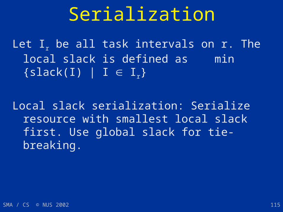
Local-Slack Resource Serialization
Let Ir be all task intervals on r. The local slack is defined as min {slack(I) | I Ir}
Local slack serialization: Serialize resource with smallest local slack first. Use global slack for tie-breaking.
SMA / CS © NUS 2002 116
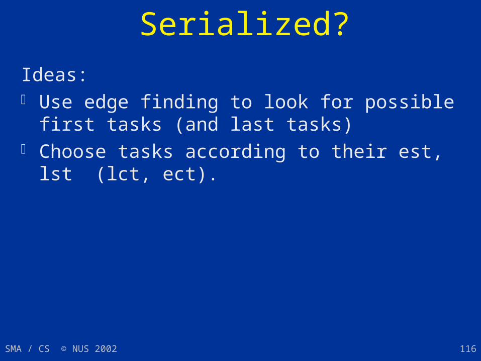
Which Tasks Are Serialized?
Ideas: Use edge finding to look for possible first tasks (and last
tasks) Choose tasks according to their est, lst (lct, ect).
SMA / CS © NUS 2002 117
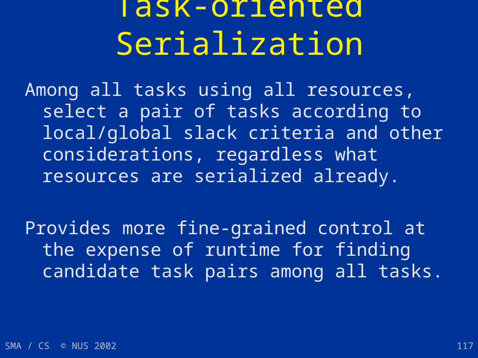
Task-oriented SerializationAmong all tasks using all resources, select a pair of
tasks according to local/global slack criteria and other considerations, regardless what resources are serialized already.
Provides more fine-grained control at the expense of runtime for finding candidate task pairs among all tasks.
SMA / CS © NUS 2002 118
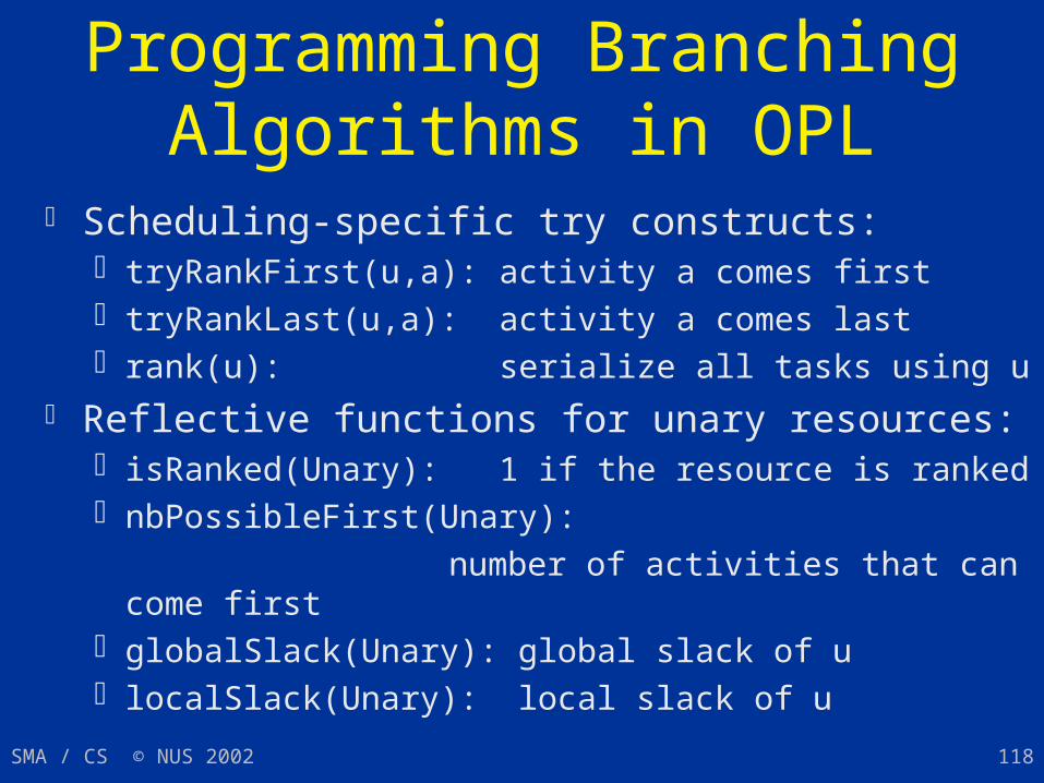
Programming Branching Algorithms in OPL
Scheduling-specific try constructs: tryRankFirst(u,a): activity a comes first tryRankLast(u,a): activity a comes last rank(u): serialize all tasks using u
Reflective functions for unary resources: isRanked(Unary): 1 if the resource is ranked nbPossibleFirst(Unary):
number of activities that can come first globalSlack(Unary): global slack of u localSlack(Unary): local slack of u
SMA / CS © NUS 2002 119
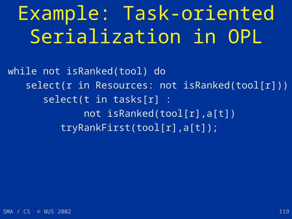
Example: Task-oriented Serialization in OPL
while not isRanked(tool) do
select(r in Resources: not isRanked(tool[r]))
select(t in tasks[r] :
not isRanked(tool[r],a[t])
tryRankFirst(tool[r],a[t]);
SMA / CS © NUS 2002 120
Demo: Serialization Algorithms
Bridge

SMA / CS © NUS 2002 121
Scheduling
Scheduling Problems Propagation Algorithms for Resource
Constraints Branching Algorithms Literature
SMA / CS © NUS 2002 122
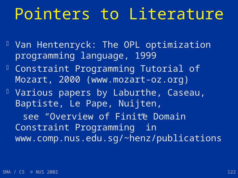
Pointers to Literature
Van Hentenryck: The OPL optimization programming language, 1999
Constraint Programming Tutorial of Mozart, 2000 (www.mozart-oz.org)
Various papers by Laburthe, Caseau, Baptiste, Le Pape, Nuijten,
see “Overview of Finite Domain Constraint Programming” in www.comp.nus.edu.sg/~henz/publications
SMA / CS © NUS 2002 123
Overview
Constraint programming in a nutshell Elements of constraint programming Sport tournament scheduling Production scheduling Assessment
SMA / CS © NUS 2002 124
Assessment: Don’t Use It!Don’t use constraint programming for: Problems for which there are known efficient algorithms
or heuristics. Example: Traveling salesman. Problems for which integer programming works well.
Example: Many discrete assignment problems. Problems with weak constraints and a complex
optimization function. Example: many timetabling problems.
SMA / CS © NUS 2002 125
Assessment: Do Use It!Use constraint programming for: Problems for which integer programming does not work
(linear models too large). Problems for which there are no efficient solutions
available. Problems with tight constraints, where propagation can be
employed. Example: ACC 97/98. Problems for which strong branching algorithms exist.
Example: Scheduling with unary resources.
SMA / CS © NUS 2002 126
Myths Debunked
A fad! Constraint programming has been used successfully in a number of application areas, most spectacularly in scheduling
Universal! More failure stories than success stories. All new! Many ideas come from AI search and Operations
Research. In particular, the important ideas for scheduling come from OR.
Artificial Intelligence! All quite earthly algorithms. Constraint programming systems provide framework for different kinds of algorithms to interact.
SMA / CS © NUS 2002 127
The Future
In OR, constraint programming is being added as a standard technique for solving combinatorial problems, along with local search (“heuristic approach”).
Constraint programming techniques will be tightly integrated with integer programming and local search.
Look at the Workshop Series on Integration of AI and OR Techniques for Combinatorial Optimization Problems (CP-AI-OR)