event history models: cox & discrete time models sociology 229: advanced regression class 6...
TRANSCRIPT

Event History Models:Cox & Discrete Time Models
Sociology 229: Advanced RegressionClass 6
Copyright © 2010 by Evan SchoferDo not copy or distribute without permission

Announcements
• Assignment 4 Handed out• More complex EHA assignment
• Today’s agenda• Cox models• Parametric Models• Reading Discussion
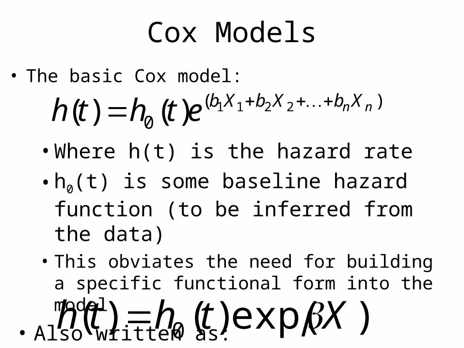
Cox Models• The basic Cox model:
)(0
2211)()( nnXbXbXbethth
• Where h(t) is the hazard rate
• h0(t) is some baseline hazard function (to be inferred from the data)
• This obviates the need for building a specific functional form into the model
• Also written as:
)exp()()( 0 Xthth

Cox Model: Example• Mostly similar to exponential model…Cox regression -- Breslow method for ties
No. of subjects = 92 Number of obs = 1938No. of failures = 77Time at risk = 1938 Wald chi2(6) = 65.49Log pseudolikelihood = -287.27209 Prob > chi2 = 0.0000
(Std. Err. adjusted for 92 clusters in newid3)------------------------------------------------------------------------------ | Robust _t | Coef. Std. Err. z P>|z| [95% Conf. Interval]-------------+---------------------------------------------------------------- gdp | .4572288 .2025104 2.26 0.024 .0603157 .8541419 degradation | -.4311475 .1131853 -3.81 0.000 -.6529867 -.2093083 education | .0027517 .0136965 0.20 0.841 -.024093 .0295964 democracy | .2836321 .0911985 3.11 0.002 .1048862 .4623779 ngo | .2874221 .1614045 1.78 0.075 -.0289248 .603769 ingo | -.026845 .2391101 -0.11 0.911 -.4954922 .4418021
Most effects = similar… though education effect loses significance…

Cox Model: Baseline Hazard
• Cox models involve a “baseline hazard”• Note: baseline = when all covariates are zero• Question: What does the baseline hazard look like?
– Or baseline survivor & integrated hazard?
– Stata can estimate the baseline survivor, hazard, integrated hazard. Two steps:
• 1. You must ask stata to save the info when you run the Cox model
– Ex: stcox gdp degradation education democracy ngo ingo, robust nohr basehc(h0)
• 2. Use “stcurve” command to plot the baseline curves– Ex: stcurve, hazard OR stcurve, survival

Cox Model: Baseline Hazard
• Baseline rate: Adoption of environmental law0
.02
.04
.06
.08
Sm
ooth
ed
haza
rd fu
nctio
n
1970 1980 1990 2000analysis time
Cox proportional hazards regression

Cox Model: Baseline Hazard
• Note: It may not always make sense to plot the baseline hazard
• Baseline shows hazard when X variables are zero• Sometimes zero values aren’t very useful/interesting
– Example: Does it make sense to plot hazard of countries adopting laws, if X vars = zero?
• Hazard rate might be quite low• In some cases, you’ll just get a flat zero curve
– Or extremely high values
– Solutions:• 1. Rescale indep vars before running cox model• 2. Use stcurve to choose relevant values of vars.

Cox Model: Estimated Hazards
• You can also use stcurve to plot estimated hazard rates based on values of indep vars
• Ex: What is hazard curve if democracy = 1, 5, 10?
• Strategy: use “at” subcommand:• stcurve , hazard at(democ=1) at2(democ=10) • NOTE: All other variables are pegged at the mean…

Cox: Estimated Hazard Rate
• Hazard rate for adoption of environmental law0
.2.4
.6.8
Sm
ooth
ed
haza
rd fu
nctio
n
1970 1980 1990 2000analysis time
democracy=1 democracy=10
Cox proportional hazards regression

Cox Model Diagnostics
• Issues that you must deal with:• 1. How to estimate results with “ties” in your data
– Ties = cases that fail at the exact same time
• 2. How to identify violations of the proportional hazard assumption
• 3. Dealing with outliers/influential cases• 4. Assessing model fit
– Most of this applies to parametric models• Ties are not a concern• But, additional issues come up: choosing the right
functional form (shape) to model the hazard.

Cox Model Issues: Ties
• How to handle ties in data• It is mathematically complex to estimate models when
there are tied failures– That is: two cases that have events at the exact same time
• Several mathematical approaches:– Breslow approximation – simplest approach
• Stata default, but not the best choice!
– Efron approximation – generally better• More computationally intensive, but given the power of
modern computers it is not an issue• stcox var1 var2 var3, efron

Cox Model Issues: Ties– Exact marginal – “continuous time approximation”
– Box-Steffensmeier & Jones: “Averaged Likelihood”
• Assumes ties didn’t happen EXACTLY at the same time… and considers all possible orderings
– Exact partial – “discrete”– Box-Steffensmeier & Jones: “exact discrete method”
• Assumes ties happened EXACTLY at the same time
– Advice:• Use Efron at a minimum• Exact methods are often more accurate
– Exact marginal often makes most sense… events rarely occur at the EXACT same time… unless you have discrete data
– But, exact methods can take a LONG time.– For big datasets with many ties, Efron is OK.

Proportional Hazard Assumption
• Key assumption: Proportional hazards• Estimated Hazard ratios are proportional over time• i.e., Estimates of a hazard ratio do NOT vary over time
– Example: Effect of “abstinence” program on sexual behavior
• Issue: Do abstinence programs lower the rate in a consistent manner across time?
– Or, perhaps the rate is lower initially… but then the rate jumps back up (maybe even exceeds the control group).
– Groups are assumed to have “parallel” hazards• Rather than rates that diverge, converge (or cross).

Proportional Hazard Assumption
• Strategies:
• 1. Visually examine raw hazard plots for sub-groups in your data
• Watch for non-parallel trends• A crude method… not the best approach… but often
identifies big violations

Proportional Hazard Assumption• Visual examination of raw hazard rate
0.0
5.1
.15
1970 1980 1990 2000analysis time
west = 0 west = 1
Smoothed hazard estimates, by west
You want them to change proportionally
If one doubles, so does the other…

Proportional Hazard Assumption
• 2. Plot –ln(-ln(survival plot)) versus ln(time) across values of X variables
• What stata calls “stphplot”• Parallel lines indicate proportional hazards• Again, convergence and divergence (or crossing)
indicates violation
– A less-common approach: compare observed survivor plot to predicted values (for different values of X)
• What stata calls “stcoxkm”• If observed are similar to predicted, assumption is not
likely to be violated.

Proportional Hazard Assumption• -ln(-ln(survivor)) vs. ln(time) – “stphplot”
Parallel=good
Convergence suggests violation of proportional hazard assumption
(But, I’ve seen worse!)
-10
12
34
-ln[-
ln(S
urv
ival
Pro
babi
lity)
]
7.585 7.59 7.595 7.6 7.605ln(analysis time)
west = 0 west = 1
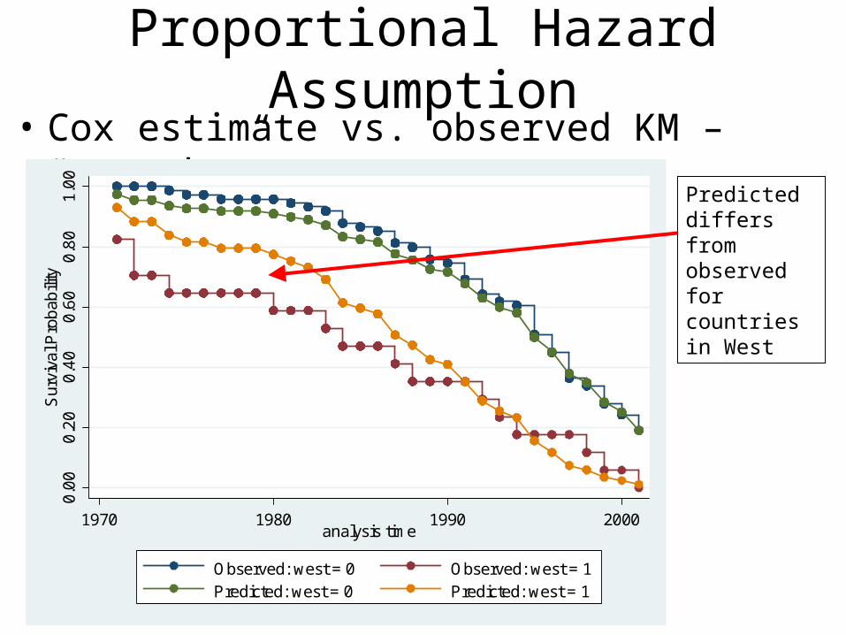
Proportional Hazard Assumption• Cox estimate vs. observed KM – “stcoxkm”
0.0
00.
20
0.4
00.
60
0.8
01.
00
Sur
viva
l Pro
bab
ility
1970 1980 1990 2000analysis time
Observed: west = 0 Observed: west = 1Predicted: west = 0 Predicted: west = 1
Predicted differs from observed for countries in West

Proportional Hazard Assumption
• 3. Piecewise Models• Piecewise = break model up into pieces (by time)
– Ex: Split analysis in to “early” vs “late” time
• If coefficients vary in different time periods, hazards are not proportional
– Example:• stcox var1 var2 var3 if _t < 10 • stcox var1 var2 var3 if _t >= 10 • Look for large changes in coefficients!
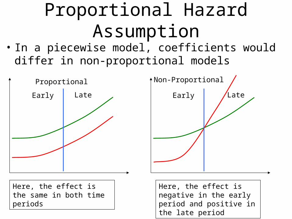
Proportional Hazard Assumption
• In a piecewise model, coefficients would differ in non-proportional models
Proportional Non-Proportional
Here, the effect is the same in both time periods
Early Late Early Late
Here, the effect is negative in the early period and positive in the late period

Piecewise Models• Look at coefficients at 2 (or more) spans of timeEARLY. stcox gdp degradation education democracy ngo ingo if year < 1985, robust nohr _t | Coef. Std. Err. z P>|z| [95% Conf. Interval]-------------+---------------------------------------------------------------- gdp | .4465818 .4255587 1.05 0.294 -.3874979 1.280661 degradation | -.282548 .1572746 -1.80 0.072 -.5908005 .0257045 education | -.0195118 .0328195 -0.59 0.552 -.0838368 .0448131 democracy | .2295673 .2625205 0.87 0.382 -.2849634 .744098 ngo | .6792462 .3110294 2.18 0.029 .0696399 1.288853 ingo | .6664661 .4804229 1.39 0.165 -.2751456 1.608078------------------------------------------------------------------------------LATE. stcox gdp degradation education democracy ngo ingo if year >= 1985, robust nohr _t | Coef. Std. Err. z P>|z| [95% Conf. Interval]-------------+---------------------------------------------------------------- gdp | .4963942 .357739 1.39 0.165 -.2047613 1.19755 degradation | -.5702894 .2395257 -2.38 0.017 -1.039751 -.1008277 education | .0142118 .0143762 0.99 0.323 -.0139649 .0423886 democracy | .2541799 .0981386 2.59 0.010 .0618317 .4465281 ngo | .1742862 .1448187 1.20 0.229 -.1095532 .4581256 ingo | -.1134661 .2104308 -0.54 0.590 -.5259028 .2989707------------------------------------------------------------------------------
Note: Effect of ngo is larger in early period

Proportional Hazard Assumption
• 4. Tests based on re-estimating model• Try including time interactions in your model• Recall: Interactions – effect of A on C varies with B• If effect of variable X on hazard rate (or ratio) varies
with time, then hazards aren’t proportional
– Recall example: Abstinence programs• Perhaps abstinence programs have a big effect initially,
but the effect diminishes (or reverses) later on

Proportional Hazard Assumption
• Red = Abstinence group; green = control
No time interaction Positive timeinteraction
In non-proportional case, the effect of abstinence programs varies across time
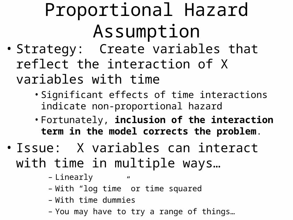
Proportional Hazard Assumption
• Strategy: Create variables that reflect the interaction of X variables with time
• Significant effects of time interactions indicate non-proportional hazard
• Fortunately, inclusion of the interaction term in the model corrects the problem.
• Issue: X variables can interact with time in multiple ways…
– Linearly– With “log time” or time squared– With time dummies– You may have to try a range of things…

Proportional Hazard Assumption
• Red = Abstinence group; green = control
Linear time interactionEffect grows consistently over timeTry “Abstinence*time”
Interaction with time-period… Effect differs early vs. late Try “Abstinence*DLate”

Proportional Hazard Assumption
• 5. Grambsch & Therneau test – Ex: Stata “estat phtest”
• Test for non-zero slope of Schoenfeld residuals vs time– Implies log hazard ratio function = proportional
• Can be applied to general model, or for each variable
stcox gdp degradation education democracy ngo ingo, robust nohr scaledsch(sca*) schoenfeld(sch*)
. estat phtest
Test of proportional hazards assumption
Time: Time ---------------------------------------------------------------- | chi2 df Prob>chi2 ------------+--------------------------------------------------- global test | 18.14 6 0.0059 ----------------------------------------------------------------
Significant chi-square indicates violation of proportional hazard assumption

Proportional Hazard Assumption
• Variable-by-variable test “estat phtest”:
. estat phtest, detail
Test of proportional hazards assumption
Time: Time ---------------------------------------------------------------- | rho chi2 df Prob>chi2 ------------+--------------------------------------------------- gdp | 0.09035 0.63 1 0.4277 degradation | -0.22735 3.41 1 0.0646 education | 0.06915 0.47 1 0.4950 democracy | -0.04929 0.20 1 0.6560 ngo | -0.18691 4.56 1 0.0327 ingo | -0.03759 0.34 1 0.5609 ------------+--------------------------------------------------- global test | 18.14 6 0.0059 ----------------------------------------------------------------
Note: Certain variables are especially problematic…

Proportional Hazard Assumption• Notes on estat phtest :
– 1. STATA 9/10: Requires that you calculate “schoenfeld residuals” when you run the original cox model
– And, if you want a test for each variable, you must also request scaled schoenfeld residuals
– 2. Test is based on identifying non-zero time trend… but how should we characterize time?
• Options: normal/linear time, log time, time dummies, etc– Results may differ depending on your choice
– Ex: estat phtest, log – specifies “log time”
• Plot of smoothed Schoenfeld residuals can indicate best way to characterize time
– Linear trend (not a curve) indicates that time is characterized OK– Ex: estat phtest, plot(ngo) OR estat phtest, log plot(ngo)

Proportional Hazard Assumption
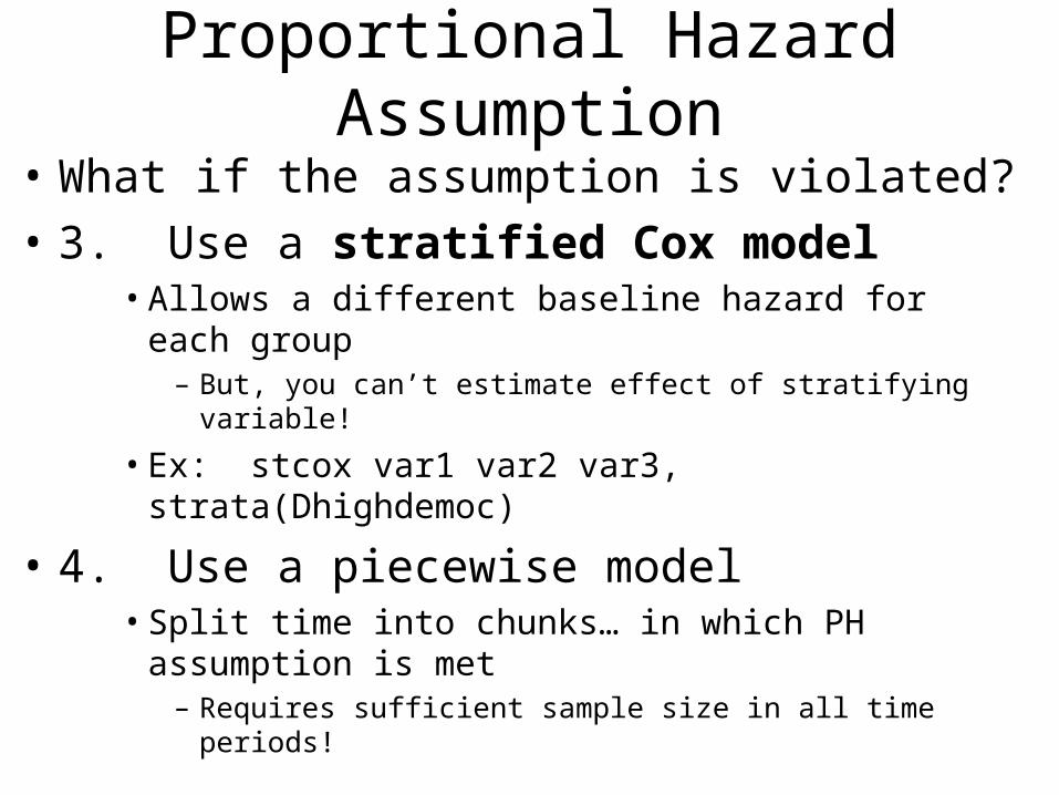
• What if the assumption is violated?
• 1. Improve model specification• Add time interactions to address nonproportionality• Ex: If high democracies are not proportional to low
democracies, try adding “highdemoc*time”• Variables can be interacted with linear time, log time,
time dummies, etc., to address the issue
• 2. Model groups separately• Split sample along variables that are non-proportional.
Proportional Hazard Assumption
• What if the assumption is violated?
• 3. Use a stratified Cox model• Allows a different baseline hazard for each group
– But, you can’t estimate effect of stratifying variable!
• Ex: stcox var1 var2 var3, strata(Dhighdemoc)
• 4. Use a piecewise model• Split time into chunks… in which PH assumption is met
– Requires sufficient sample size in all time periods!

Proportional Hazard Assumption
• What if the assumption is violated?
• 5. Live with it (but temper your conclusions)• Violation of proportional hazard assumption tends to:
– Overestimate the effect of variables whose hazard ratios are increasing over time
– And, underestimate those whose hazard ratios are decreasing
• However, Allison points out: Cox model is reasonably robust
– Other issues (e.g., model misspecification) are bigger issues
Discrete Time EHA Models
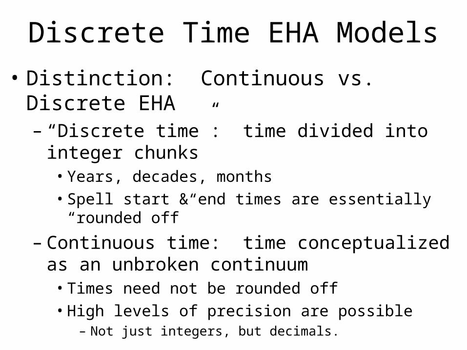
• Distinction: Continuous vs. Discrete EHA– “Discrete time”: time divided into integer chunks
• Years, decades, months• Spell start & end times are essentially “rounded off”
– Continuous time: time conceptualized as an unbroken continuum
• Times need not be rounded off• High levels of precision are possible
– Not just integers, but decimals.

Discrete Time EHA Models
• Issue: Discrete vs. continuous time gives rise to different EHA models
• Example: The hazard rate is defined for continuous time:
t
tTtTttPth
t
)(lim)(
0
• The hazard rate over discrete (identical-sized) chunks of time is (ti):
ii tTtTPth )(

Discrete Time EHA Models
• Issue: If the hazard rate in discrete time is a probability, maybe we can model it as such…– Standard options for modeling probabilities:
• Logistic regression (logit) model• Probit model• Complementary log/log model (cloglog)
– An asymmetric function– Starts slowly from p=0, but accelerates more rapidly toward
p=1 at the end– Often used when predicted probabilities are very low or high.

Discrete Time EHA Models
• Example: Discrete time logit model
Xap
pLogitth
1
log)(
• Where p is the probability of an event (Y=1) for a discrete chunk of time
• Complementary log log model looks like this:
Xapth 1loglog)(
Discrete Time EHA Models
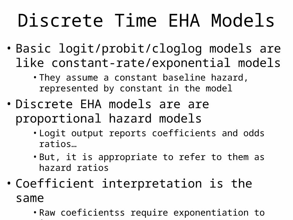
• Basic logit/probit/cloglog models are like constant-rate/exponential models
• They assume a constant baseline hazard, represented by constant in the model
• Discrete EHA models are are proportional hazard models
• Logit output reports coefficients and odds ratios…• But, it is appropriate to refer to them as hazard ratios
• Coefficient interpretation is the same• Raw coeficientss require exponentiation to interpret…

Discrete Time EHA: Data
• Discrete time models require split-spell data where each spell has constant length
• Example: every record in your data represents 1 year• Number of cases represents total time at risk
– Ex: If caseid 1 has 10 records, it was at risk for 10 years…
• This differs from continuous models, where records can represent variable amounts of time
– E.g., by providing specific start and end times…

Discrete Time EHA Data
• Discrete time data looks like other examples of split spell data
• But, each record MUST be the same length
– Example: Country data over time:• Logit/probit/cloglog simply models outcome of 1
newname2 newid3 year law eventnum start end ss es popINDIA 1119 1978 0 1 1978 1979 0 0 656941INDIA 1119 1979 0 1 1979 1980 0 0 672021INDIA 1119 1980 0 1 1980 1981 0 0 687332INDIA 1119 1981 0 1 1981 1982 0 0 702821INDIA 1119 1982 0 1 1982 1983 0 0 718426INDIA 1119 1983 0 1 1983 1984 0 0 734072INDIA 1119 1984 0 1 1984 1985 0 0 749677INDIA 1119 1985 0 1 1985 1986 0 0 765147INDIA 1119 1986 1 1 1986 1987 0 1 781893
Event (Y=1)

Discrete Time Logit Model• Logit model for discrete time EHA
• It is a constant rate model• In fact, results are almost the same as streg…
. logit es gdp degradation education democracy ngo ingo
Logistic regression Number of obs = 1938 LR chi2(6) = 47.83 Prob > chi2 = 0.0000Log likelihood = -299.90676 Pseudo R2 = 0.0739
------------------------------------------------------------------------------ es | Coef. Std. Err. z P>|z| [95% Conf. Interval]-------------+---------------------------------------------------------------- gdp | -.02752 .2274919 -0.12 0.904 -.473396 .4183559 degradation | -.5264763 .1404763 -3.75 0.000 -.8018049 -.2511477 education | .0415878 .0141799 2.93 0.003 .0137957 .0693799 democracy | .2429383 .0981245 2.48 0.013 .0506179 .4352587 ngo | .4534059 .177047 2.56 0.010 .1064001 .8004117 ingo | .3298737 .2341225 1.41 0.159 -.128998 .7887455 _cons | -4.724106 1.916741 -2.46 0.014 -8.48085 -.9673627------------------------------------------------------------------------------

Discrete Time and Cox Models
• A Cox model can also be estimated in the discrete time context
• Indeed, the discrete time example helps illustrate what a Cox model really is (even in continuous time)
– Idea: Use a conditional logit model• Conditioned on the cases in the risk set at each point in
time• … rather than a traditional logit model

Discrete Time and Cox Models
• A conditional logit model estimates common coefficients across models for many groups
• Looks at within-group factors, net of overall rate within each group… sorta like a fixed-effects model…
– Box-Steffensmeier & Jones, p. 80
• Thus, effects are modeled net of the “baseline hazard”
– Interpretation: A Cox model is like pooling a large set of logit results
• In the continuous time context, the group is the current risk set at the time of any failure

Discrete Time and Cox Models
• A conditional logit model on discrete time EHA yields identical results to a Cox Model;
• If you specify the “exact partial” method for handling ties in the continuous time Cox model
– We’ll cover this later

Discrete Time Cox Model• Conditional logit model – a cox model
• Yields identical results to cox when using discrete data
. clogit es gdp degradation education democracy ngo ingo, group(year)
Conditional (fixed-effects) logistic regression Number of obs = 1472 LR chi2(6) = 25.49 Prob > chi2 = 0.0003Log likelihood = -224.89587 Pseudo R2 = 0.0536
------------------------------------------------------------------------------ es | Coef. Std. Err. z P>|z| [95% Conf. Interval]-------------+---------------------------------------------------------------- gdp | .4806954 .2499626 1.92 0.054 -.0092223 .9706132 degradation | -.4624672 .1502146 -3.08 0.002 -.7568824 -.168052 education | .0036883 .0148541 0.25 0.804 -.0254251 .0328017 democracy | .3066401 .0971026 3.16 0.002 .1163225 .4969578 ngo | .314372 .1715222 1.83 0.067 -.0218052 .6505493 ingo | -.0329307 .2009382 -0.16 0.870 -.4267624 .360901------------------------------------------------------------------------------

Discrete vs. Continuous EHA
• In practice, we can often use either discrete or continuous methods
• Even though time is theoretically continuous, our measures are usually limited to discrete time intervals
– Ex: year, month, day…
• For yearly spell data (or any other consistent interval) the data sets are pretty much identical
– If time resolution is extremely poor, there can be advantages to using discrete time models
– Otherwise, continuous time models provide greater flexibility
• And more modeling options.

EHA Example
• In-class group activity: Let’s design a study• Outcome of interest: Students dropping a course• What is the risk set?• How would you set up the data?• What are key independent variables?• What kind of model would you use?• Work in groups of 2-4, and be prepared to discuss your
thoughts…

Reading Discussion
• Empirical Example: Soule, Sarah A and Susan Olzak. 2004. “When Do Movements Matter? The Politics of Contingency and the Equal Rights Amendment.” American Sociological Review, Vol. 69, No. 4. (Aug., 2004), pp. 473-497.
• Long, J. Scott, Paul D. Allison, and Robert McGinnis. 1993. “Rank Advancement in Academic Careers: Sex Differences and the Effects of Productivity.” American Sociological Review, 58, 5:703-722.
