event history models 2 sociology 229a: event history analysis class 4 copyright © 2008 by evan...
Post on 22-Dec-2015
228 views
TRANSCRIPT
Event History Models 2
Sociology 229A: Event History AnalysisClass 4
Copyright © 2008 by Evan SchoferDo not copy or distribute without permission
Announcements
• Assignment 2 due• Assignment # handed out
• Agenda• More EHA models• Discrete time models• More details on Cox models & other fully parametric
Proportional Hazard models• Break• Discussion of paper: Allison and McGinnis
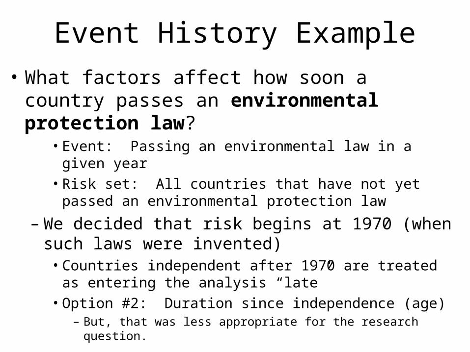
Event History Example
• What factors affect how soon a country passes an environmental protection law?
• Event: Passing an environmental law in a given year• Risk set: All countries that have not yet passed an
environmental protection law
– We decided that risk begins at 1970 (when such laws were invented)
• Countries independent after 1970 are treated as entering the analysis “late”
• Option #2: Duration since independence (age)– But, that was less appropriate for the research question.
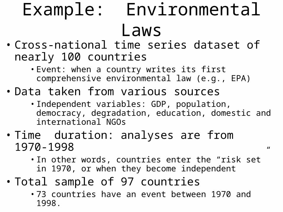
Example: Environmental Laws• Cross-national time series dataset of nearly
100 countries• Event: when a country writes its first comprehensive
environmental law (e.g., EPA)
• Data taken from various sources• Independent variables: GDP, population, democracy,
degradation, education, domestic and international NGOs
• Time duration: analyses are from 1970-1998• In other words, countries enter the “risk set” in 1970, or
when they become independent
• Total sample of 97 countries• 73 countries have an event between 1970 and 1998.
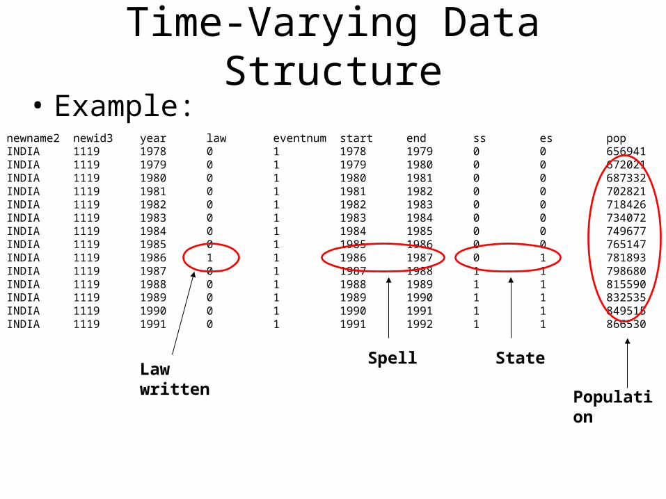
Time-Varying Data Structure
newname2 newid3 year law eventnum start end ss es popINDIA 1119 1978 0 1 1978 1979 0 0 656941INDIA 1119 1979 0 1 1979 1980 0 0 672021INDIA 1119 1980 0 1 1980 1981 0 0 687332INDIA 1119 1981 0 1 1981 1982 0 0 702821INDIA 1119 1982 0 1 1982 1983 0 0 718426INDIA 1119 1983 0 1 1983 1984 0 0 734072INDIA 1119 1984 0 1 1984 1985 0 0 749677INDIA 1119 1985 0 1 1985 1986 0 0 765147INDIA 1119 1986 1 1 1986 1987 0 1 781893INDIA 1119 1987 0 1 1987 1988 1 1 798680INDIA 1119 1988 0 1 1988 1989 1 1 815590INDIA 1119 1989 0 1 1989 1990 1 1 832535INDIA 1119 1990 0 1 1990 1991 1 1 849515INDIA 1119 1991 0 1 1991 1992 1 1 866530
• Example:
Law writtenSpell State
Population
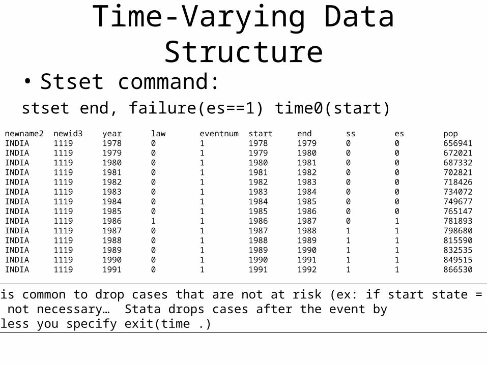
Time-Varying Data Structure
newname2 newid3 year law eventnum start end ss es popINDIA 1119 1978 0 1 1978 1979 0 0 656941INDIA 1119 1979 0 1 1979 1980 0 0 672021INDIA 1119 1980 0 1 1980 1981 0 0 687332INDIA 1119 1981 0 1 1981 1982 0 0 702821INDIA 1119 1982 0 1 1982 1983 0 0 718426INDIA 1119 1983 0 1 1983 1984 0 0 734072INDIA 1119 1984 0 1 1984 1985 0 0 749677INDIA 1119 1985 0 1 1985 1986 0 0 765147INDIA 1119 1986 1 1 1986 1987 0 1 781893INDIA 1119 1987 0 1 1987 1988 1 1 798680INDIA 1119 1988 0 1 1988 1989 1 1 815590INDIA 1119 1989 0 1 1989 1990 1 1 832535INDIA 1119 1990 0 1 1990 1991 1 1 849515INDIA 1119 1991 0 1 1991 1992 1 1 866530
• Stset command:stset end, failure(es==1) time0(start)
Note: It is common to drop cases that are not at risk (ex: if start state = 1)BUT, it is not necessary… Stata drops cases after the event by default…unless you specify exit(time .)
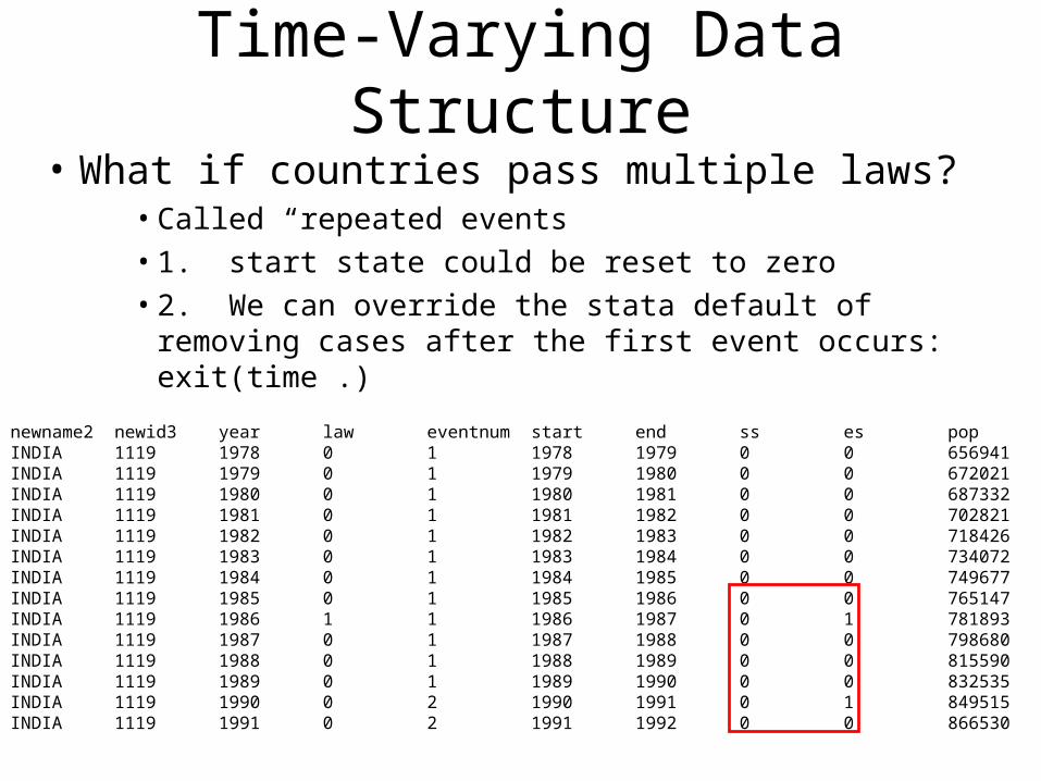
Time-Varying Data Structure
• What if countries pass multiple laws?• Called “repeated events• 1. start state could be reset to zero• 2. We can override the stata default of removing
cases after the first event occurs: exit(time .)
newname2 newid3 year law eventnum start end ss es popINDIA 1119 1978 0 1 1978 1979 0 0 656941INDIA 1119 1979 0 1 1979 1980 0 0 672021INDIA 1119 1980 0 1 1980 1981 0 0 687332INDIA 1119 1981 0 1 1981 1982 0 0 702821INDIA 1119 1982 0 1 1982 1983 0 0 718426INDIA 1119 1983 0 1 1983 1984 0 0 734072INDIA 1119 1984 0 1 1984 1985 0 0 749677INDIA 1119 1985 0 1 1985 1986 0 0 765147INDIA 1119 1986 1 1 1986 1987 0 1 781893INDIA 1119 1987 0 1 1987 1988 0 0 798680INDIA 1119 1988 0 1 1988 1989 0 0 815590INDIA 1119 1989 0 1 1989 1990 0 0 832535INDIA 1119 1990 0 2 1990 1991 0 1 849515INDIA 1119 1991 0 2 1991 1992 0 0 866530
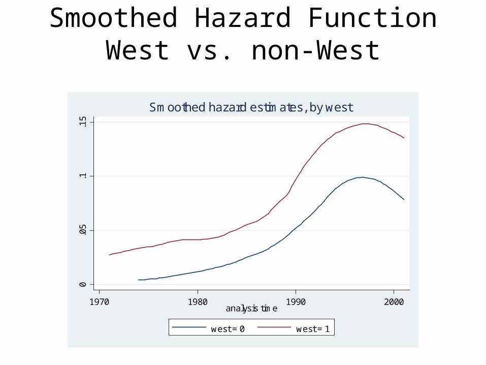
Smoothed Hazard FunctionWest vs. non-West
0.0
5.1
.15
1970 1980 1990 2000analysis time
west = 0 west = 1
Smoothed hazard estimates, by west
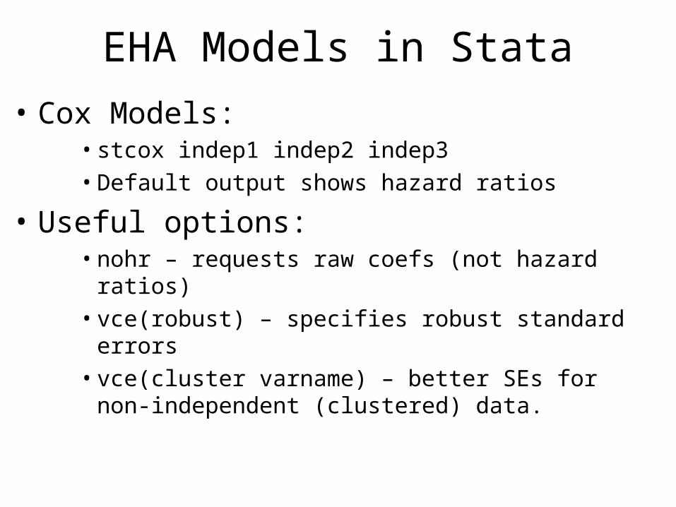
EHA Models in Stata
• Cox Models:•stcox indep1 indep2 indep3• Default output shows hazard ratios
• Useful options:•nohr – requests raw coefs (not hazard ratios)•vce(robust) – specifies robust standard errors•vce(cluster varname) – better SEs for non-
independent (clustered) data.
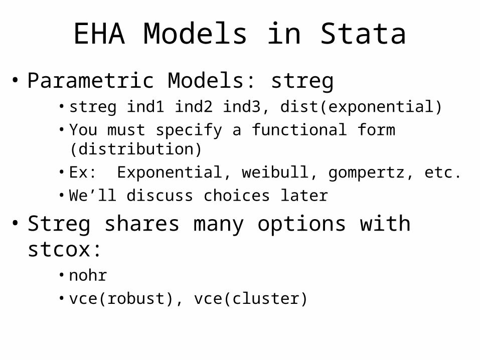
EHA Models in Stata
• Parametric Models: streg•streg ind1 ind2 ind3, dist(exponential)• You must specify a functional form (distribution)• Ex: Exponential, weibull, gompertz, etc.• We’ll discuss choices later
• Streg shares many options with stcox:• nohr• vce(robust), vce(cluster)
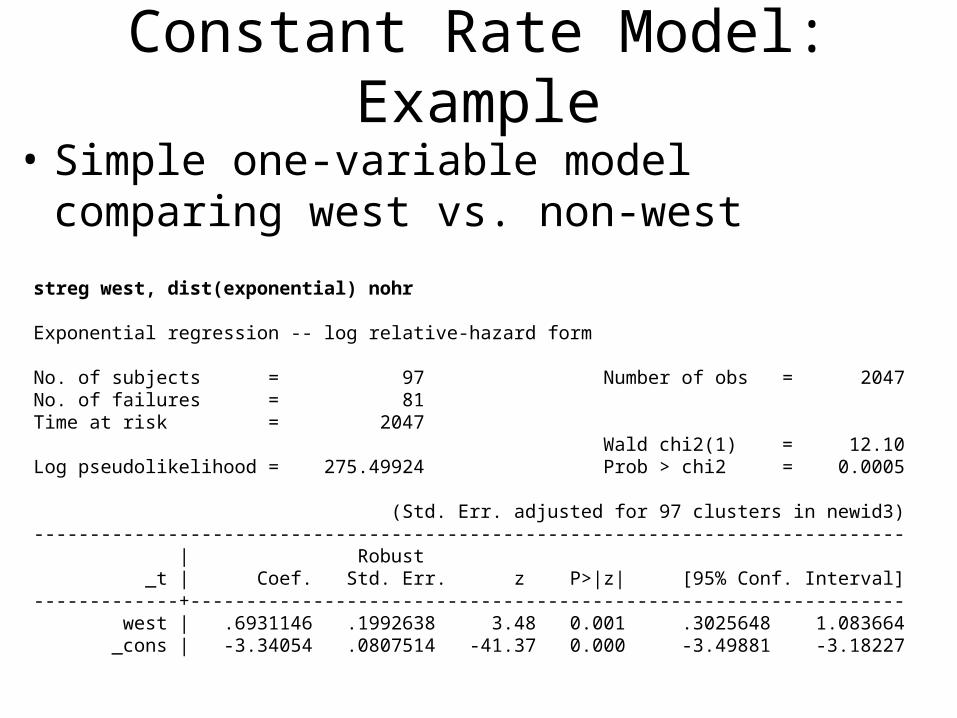
Constant Rate Model: Example
• Simple one-variable model comparing west vs. non-west
streg west, dist(exponential) nohr
Exponential regression -- log relative-hazard form
No. of subjects = 97 Number of obs = 2047No. of failures = 81Time at risk = 2047 Wald chi2(1) = 12.10Log pseudolikelihood = 275.49924 Prob > chi2 = 0.0005
(Std. Err. adjusted for 97 clusters in newid3)------------------------------------------------------------------------------ | Robust _t | Coef. Std. Err. z P>|z| [95% Conf. Interval]-------------+---------------------------------------------------------------- west | .6931146 .1992638 3.48 0.001 .3025648 1.083664 _cons | -3.34054 .0807514 -41.37 0.000 -3.49881 -3.18227
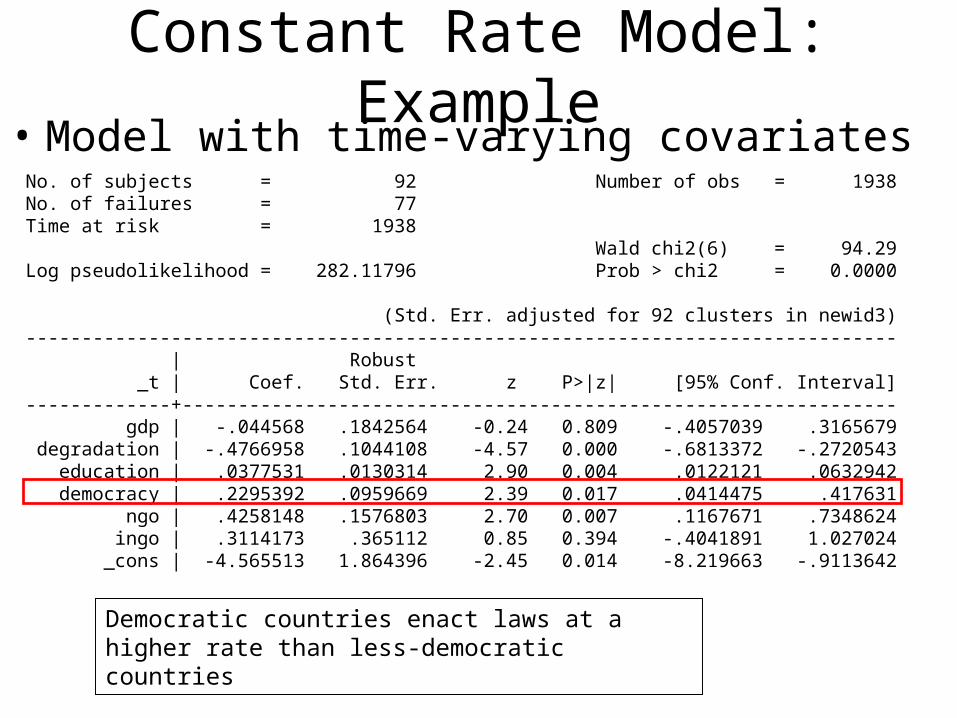
Constant Rate Model: Example• Model with time-varying covariatesNo. of subjects = 92 Number of obs = 1938No. of failures = 77Time at risk = 1938 Wald chi2(6) = 94.29Log pseudolikelihood = 282.11796 Prob > chi2 = 0.0000
(Std. Err. adjusted for 92 clusters in newid3)------------------------------------------------------------------------------ | Robust _t | Coef. Std. Err. z P>|z| [95% Conf. Interval]-------------+---------------------------------------------------------------- gdp | -.044568 .1842564 -0.24 0.809 -.4057039 .3165679 degradation | -.4766958 .1044108 -4.57 0.000 -.6813372 -.2720543 education | .0377531 .0130314 2.90 0.004 .0122121 .0632942 democracy | .2295392 .0959669 2.39 0.017 .0414475 .417631 ngo | .4258148 .1576803 2.70 0.007 .1167671 .7348624 ingo | .3114173 .365112 0.85 0.394 -.4041891 1.027024 _cons | -4.565513 1.864396 -2.45 0.014 -8.219663 -.9113642
Democratic countries enact laws at a higher rate than less-democratic countries
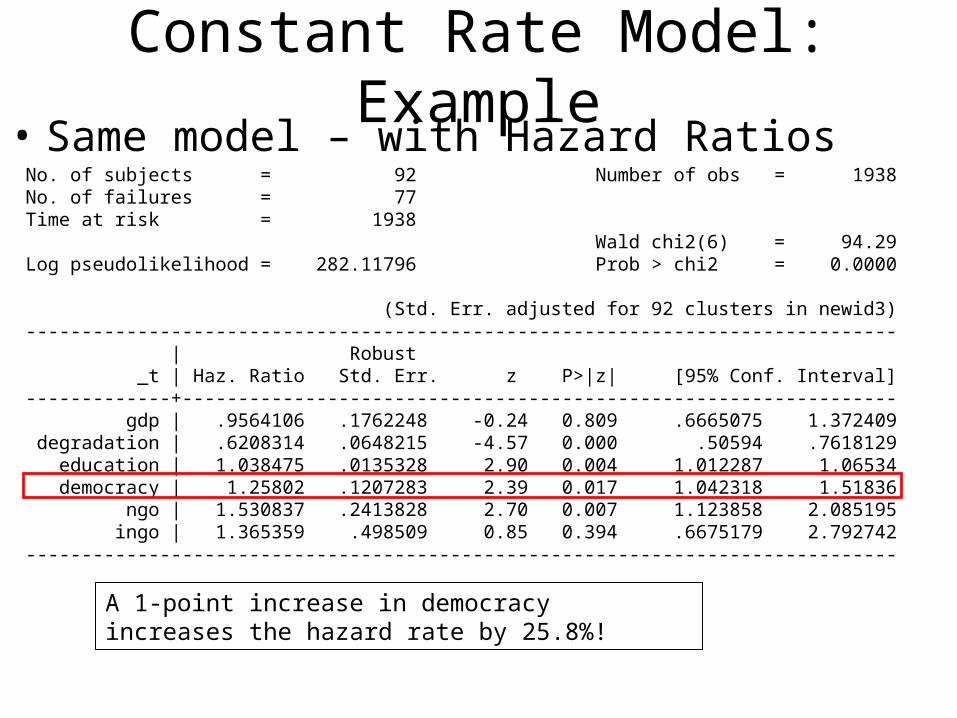
Constant Rate Model: Example• Same model – with Hazard RatiosNo. of subjects = 92 Number of obs = 1938No. of failures = 77Time at risk = 1938 Wald chi2(6) = 94.29Log pseudolikelihood = 282.11796 Prob > chi2 = 0.0000
(Std. Err. adjusted for 92 clusters in newid3)------------------------------------------------------------------------------ | Robust _t | Haz. Ratio Std. Err. z P>|z| [95% Conf. Interval]-------------+---------------------------------------------------------------- gdp | .9564106 .1762248 -0.24 0.809 .6665075 1.372409 degradation | .6208314 .0648215 -4.57 0.000 .50594 .7618129 education | 1.038475 .0135328 2.90 0.004 1.012287 1.06534 democracy | 1.25802 .1207283 2.39 0.017 1.042318 1.51836 ngo | 1.530837 .2413828 2.70 0.007 1.123858 2.085195 ingo | 1.365359 .498509 0.85 0.394 .6675179 2.792742------------------------------------------------------------------------------
A 1-point increase in democracy increases the hazard rate by 25.8%!
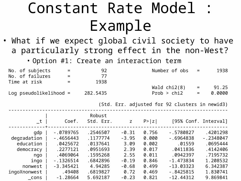
Constant Rate Model : Example
• What if we expect global civil society to have a particularly strong effect in the non-West?
• Option #1: Create an interaction termNo. of subjects = 92 Number of obs = 1938No. of failures = 77Time at risk = 1938 Wald chi2(8) = 91.25Log pseudolikelihood = 282.5435 Prob > chi2 = 0.0000
(Std. Err. adjusted for 92 clusters in newid3)------------------------------------------------------------------------------ | Robust _t | Coef. Std. Err. z P>|z| [95% Conf. Interval]-------------+---------------------------------------------------------------- gdp | -.0789765 .2546507 -0.31 0.756 -.5780827 .4201298 degradation | -.4656443 .1177774 -3.95 0.000 -.6964838 -.2348047 education | .0425672 .0137641 3.09 0.002 .01559 .0695444 democracy | .2277121 .0951693 2.39 0.017 .0411836 .4142406 ngo | .4069064 .1595268 2.55 0.011 .0942397 .7195732 ingo | -.1326514 .6842896 -0.19 0.846 -1.473834 1.208532 nonwest | -3.345421 4.94285 -0.68 0.499 -13.03323 6.342387ingoXnonwest | .49408 .6819827 0.72 0.469 -.8425815 1.830741 _cons | -1.28664 5.692187 -0.23 0.821 -12.44312 9.869841
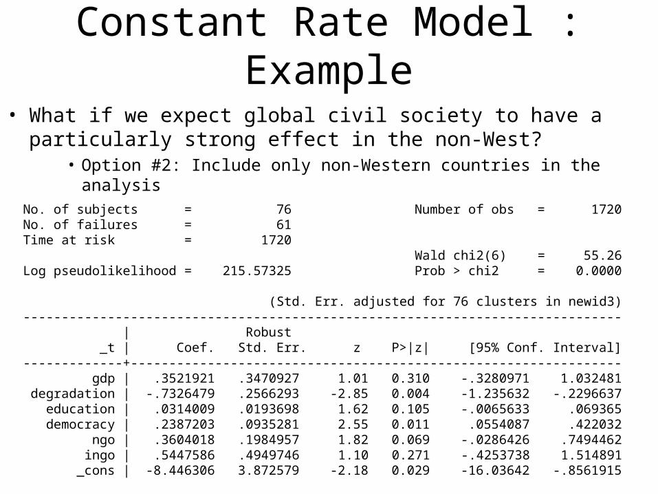
Constant Rate Model : Example
• What if we expect global civil society to have a particularly strong effect in the non-West?
• Option #2: Include only non-Western countries in the analysis
No. of subjects = 76 Number of obs = 1720No. of failures = 61Time at risk = 1720 Wald chi2(6) = 55.26Log pseudolikelihood = 215.57325 Prob > chi2 = 0.0000
(Std. Err. adjusted for 76 clusters in newid3)------------------------------------------------------------------------------ | Robust _t | Coef. Std. Err. z P>|z| [95% Conf. Interval]-------------+---------------------------------------------------------------- gdp | .3521921 .3470927 1.01 0.310 -.3280971 1.032481 degradation | -.7326479 .2566293 -2.85 0.004 -1.235632 -.2296637 education | .0314009 .0193698 1.62 0.105 -.0065633 .069365 democracy | .2387203 .0935281 2.55 0.011 .0554087 .422032 ngo | .3604018 .1984957 1.82 0.069 -.0286426 .7494462 ingo | .5447586 .4949746 1.10 0.271 -.4253738 1.514891 _cons | -8.446306 3.872579 -2.18 0.029 -16.03642 -.8561915
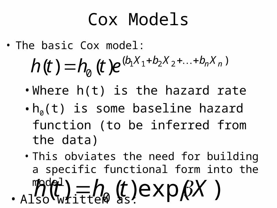
Cox Models• The basic Cox model:
)(0
2211)()( nnXbXbXbethth
• Where h(t) is the hazard rate
• h0(t) is some baseline hazard function (to be inferred from the data)
• This obviates the need for building a specific functional form into the model
• Also written as:
)exp()()( 0 Xthth
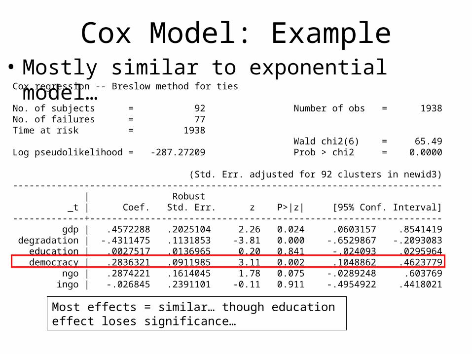
Cox Model: Example• Mostly similar to exponential model…Cox regression -- Breslow method for ties
No. of subjects = 92 Number of obs = 1938No. of failures = 77Time at risk = 1938 Wald chi2(6) = 65.49Log pseudolikelihood = -287.27209 Prob > chi2 = 0.0000
(Std. Err. adjusted for 92 clusters in newid3)------------------------------------------------------------------------------ | Robust _t | Coef. Std. Err. z P>|z| [95% Conf. Interval]-------------+---------------------------------------------------------------- gdp | .4572288 .2025104 2.26 0.024 .0603157 .8541419 degradation | -.4311475 .1131853 -3.81 0.000 -.6529867 -.2093083 education | .0027517 .0136965 0.20 0.841 -.024093 .0295964 democracy | .2836321 .0911985 3.11 0.002 .1048862 .4623779 ngo | .2874221 .1614045 1.78 0.075 -.0289248 .603769 ingo | -.026845 .2391101 -0.11 0.911 -.4954922 .4418021
Most effects = similar… though education effect loses significance…
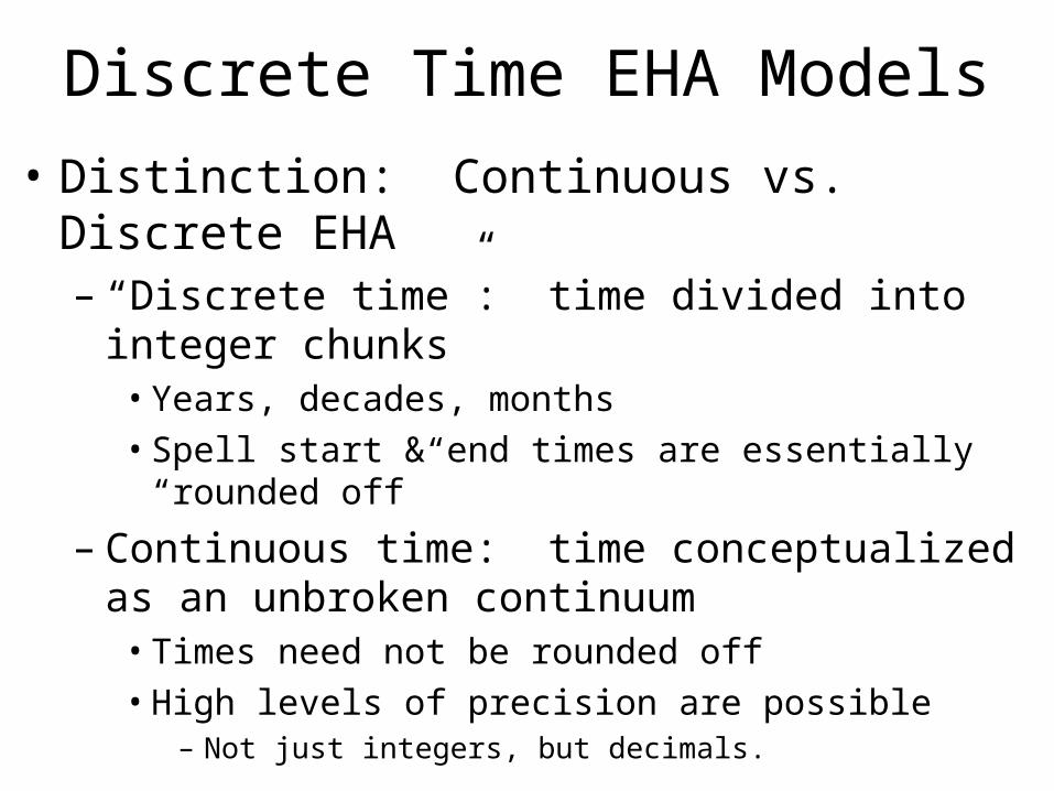
Discrete Time EHA Models
• Distinction: Continuous vs. Discrete EHA– “Discrete time”: time divided into integer chunks
• Years, decades, months• Spell start & end times are essentially “rounded off”
– Continuous time: time conceptualized as an unbroken continuum
• Times need not be rounded off• High levels of precision are possible
– Not just integers, but decimals.
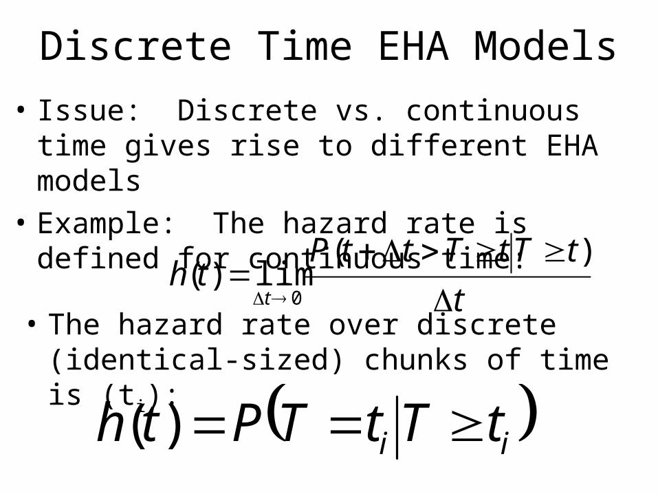
Discrete Time EHA Models
• Issue: Discrete vs. continuous time gives rise to different EHA models
• Example: The hazard rate is defined for continuous time:
t
tTtTttPth
t
)(lim)(
0
• The hazard rate over discrete (identical-sized) chunks of time is (ti):
ii tTtTPth )(
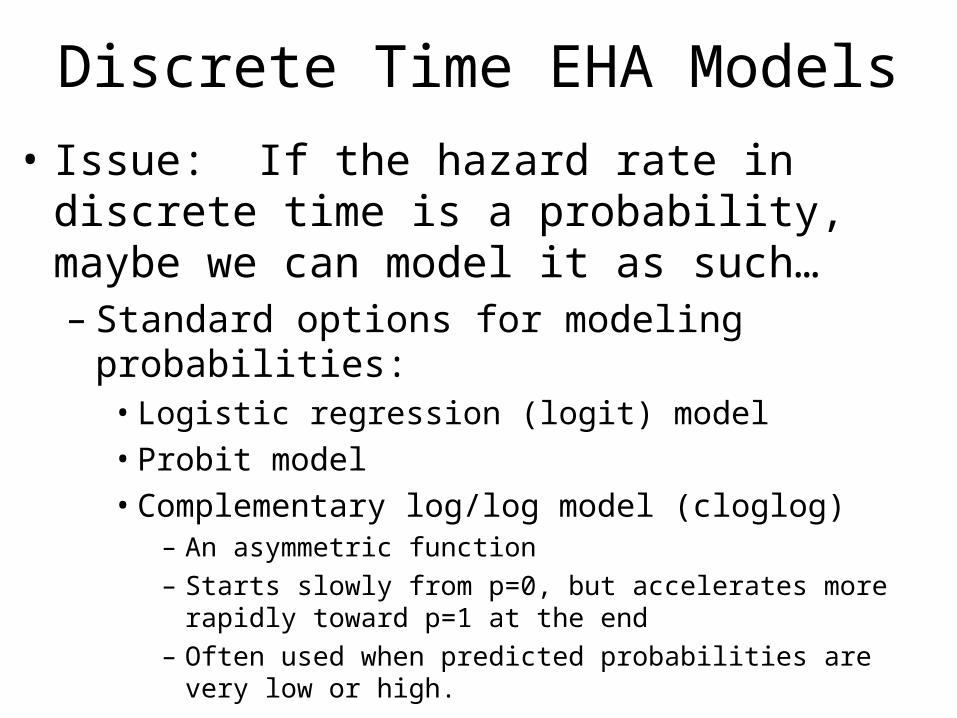
Discrete Time EHA Models
• Issue: If the hazard rate in discrete time is a probability, maybe we can model it as such…– Standard options for modeling probabilities:
• Logistic regression (logit) model• Probit model• Complementary log/log model (cloglog)
– An asymmetric function– Starts slowly from p=0, but accelerates more rapidly toward
p=1 at the end– Often used when predicted probabilities are very low or high.
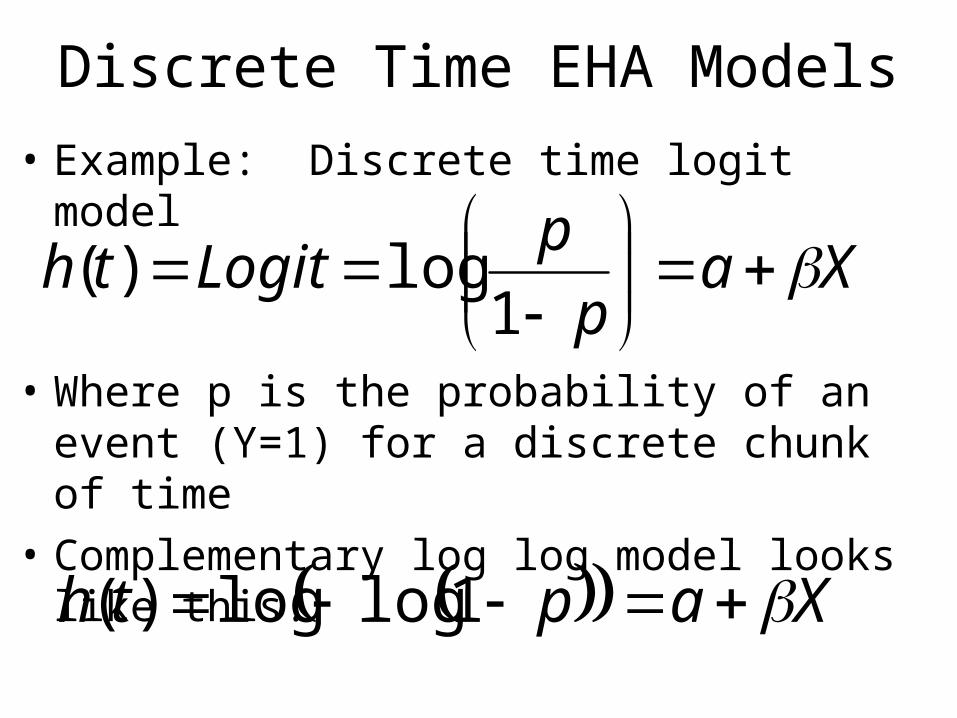
Discrete Time EHA Models
• Example: Discrete time logit model
Xap
pLogitth
1
log)(
• Where p is the probability of an event (Y=1) for a discrete chunk of time
• Complementary log log model looks like this:
Xapth 1loglog)(
Discrete Time EHA Models
• Basic logit/probit/cloglog models are like constant-rate/exponential models
• They assume a constant baseline hazard, represented by constant in the model
• Discrete EHA models are are proportional hazard models
• Logit output reports coefficients and odds ratios…• But, it is appropriate to refer to them as hazard ratios
• Coefficient interpretation is the same• Raw coeficientss require exponentiation to interpret…
Discrete Time EHA: Data
• Discrete time models require split-spell data where each spell has constant length
• Example: every record in your data represents 1 year• Number of cases represents total time at risk
– Ex: If caseid 1 has 10 records, it was at risk for 10 years…
• This differs from continuous models, where records can represent variable amounts of time
– E.g., by providing specific start and end times…
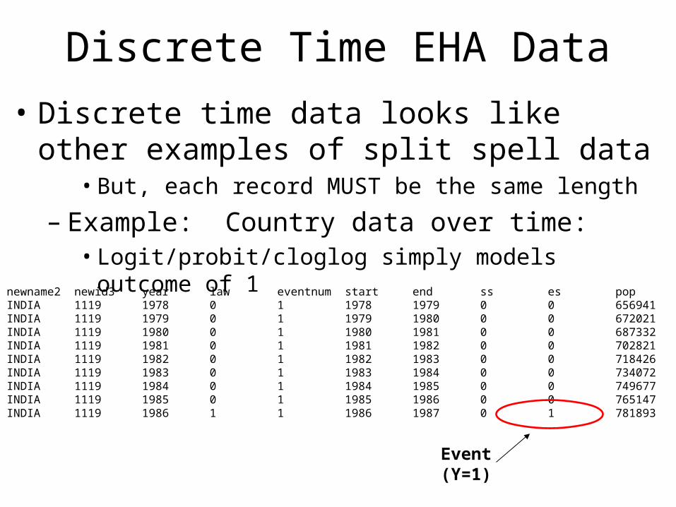
Discrete Time EHA Data
• Discrete time data looks like other examples of split spell data
• But, each record MUST be the same length
– Example: Country data over time:• Logit/probit/cloglog simply models outcome of 1
newname2 newid3 year law eventnum start end ss es popINDIA 1119 1978 0 1 1978 1979 0 0 656941INDIA 1119 1979 0 1 1979 1980 0 0 672021INDIA 1119 1980 0 1 1980 1981 0 0 687332INDIA 1119 1981 0 1 1981 1982 0 0 702821INDIA 1119 1982 0 1 1982 1983 0 0 718426INDIA 1119 1983 0 1 1983 1984 0 0 734072INDIA 1119 1984 0 1 1984 1985 0 0 749677INDIA 1119 1985 0 1 1985 1986 0 0 765147INDIA 1119 1986 1 1 1986 1987 0 1 781893
Event (Y=1)
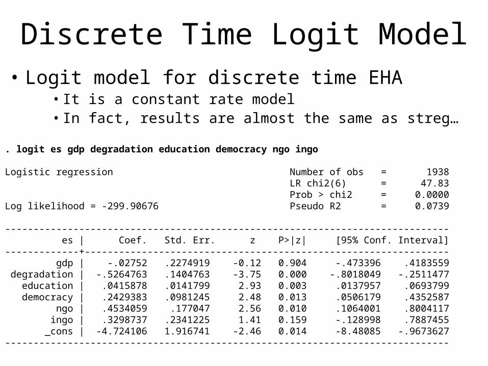
Discrete Time Logit Model• Logit model for discrete time EHA
• It is a constant rate model• In fact, results are almost the same as streg…
. logit es gdp degradation education democracy ngo ingo
Logistic regression Number of obs = 1938 LR chi2(6) = 47.83 Prob > chi2 = 0.0000Log likelihood = -299.90676 Pseudo R2 = 0.0739
------------------------------------------------------------------------------ es | Coef. Std. Err. z P>|z| [95% Conf. Interval]-------------+---------------------------------------------------------------- gdp | -.02752 .2274919 -0.12 0.904 -.473396 .4183559 degradation | -.5264763 .1404763 -3.75 0.000 -.8018049 -.2511477 education | .0415878 .0141799 2.93 0.003 .0137957 .0693799 democracy | .2429383 .0981245 2.48 0.013 .0506179 .4352587 ngo | .4534059 .177047 2.56 0.010 .1064001 .8004117 ingo | .3298737 .2341225 1.41 0.159 -.128998 .7887455 _cons | -4.724106 1.916741 -2.46 0.014 -8.48085 -.9673627------------------------------------------------------------------------------
Discrete Time and Cox Models
• A Cox model can also be estimated in the discrete time context
• Indeed, the discrete time example helps illustrate what a Cox model really is (even in continuous time)
– Idea: Use a conditional logit model• Conditioned on the cases in the risk set at each point in
time• … rather than a traditional logit model
Discrete Time and Cox Models
• A conditional logit model estimates common coefficients across models for many groups
• Looks at within-group factors, net of overall rate within each group… sorta like a fixed-effects model…
– Box-Steffensmeier & Jones, p. 80
• Thus, effects are modeled net of the “baseline hazard”
– Interpretation: A Cox model is like pooling a large set of logit results
• In the continuous time context, the group is the current risk set at the time of any failure
Discrete Time and Cox Models
• A conditional logit model on discrete time EHA yields identical results to a Cox Model;
• If you specify the “exact partial” method for handling ties in the continuous time Cox model
– We’ll cover this later
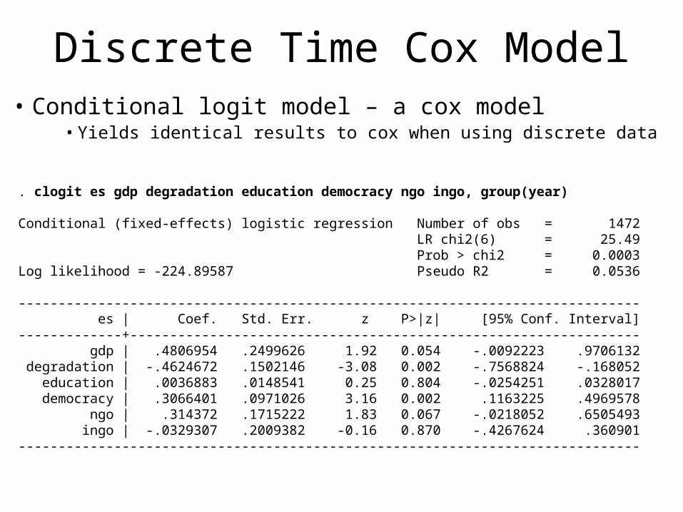
Discrete Time Cox Model• Conditional logit model – a cox model
• Yields identical results to cox when using discrete data
. clogit es gdp degradation education democracy ngo ingo, group(year)
Conditional (fixed-effects) logistic regression Number of obs = 1472 LR chi2(6) = 25.49 Prob > chi2 = 0.0003Log likelihood = -224.89587 Pseudo R2 = 0.0536
------------------------------------------------------------------------------ es | Coef. Std. Err. z P>|z| [95% Conf. Interval]-------------+---------------------------------------------------------------- gdp | .4806954 .2499626 1.92 0.054 -.0092223 .9706132 degradation | -.4624672 .1502146 -3.08 0.002 -.7568824 -.168052 education | .0036883 .0148541 0.25 0.804 -.0254251 .0328017 democracy | .3066401 .0971026 3.16 0.002 .1163225 .4969578 ngo | .314372 .1715222 1.83 0.067 -.0218052 .6505493 ingo | -.0329307 .2009382 -0.16 0.870 -.4267624 .360901------------------------------------------------------------------------------
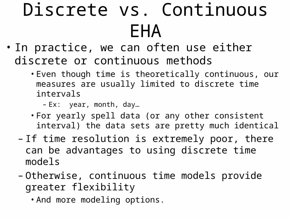
Discrete vs. Continuous EHA
• In practice, we can often use either discrete or continuous methods
• Even though time is theoretically continuous, our measures are usually limited to discrete time intervals
– Ex: year, month, day…
• For yearly spell data (or any other consistent interval) the data sets are pretty much identical
– If time resolution is extremely poor, there can be advantages to using discrete time models
– Otherwise, continuous time models provide greater flexibility
• And more modeling options.
EHA Example
• In-class group activity: Let’s design a study• Outcome of interest: Students dropping a course• What is the risk set?• How would you set up the data?• What are key independent variables?• What kind of model would you use?• Work in groups of 2-4, and be prepared to discuss your
thoughts…
Reading Discussion
• Long, J. Scott, Paul D. Allison, and Robert McGinnis. 1993. “Rank Advancement in Academic Careers: Sex Differences and the Effects of Productivity.” American Sociological Review, 58, 5:703-722.
