Hydrol. Earth Syst. Sci., 18, 3179–3193, 2014www.hydrol-earth-syst-sci.net/18/3179/2014/doi:10.5194/hess-18-3179-2014© Author(s) 2014. CC Attribution 3.0 License.

Evaluation of TRMM 3B42 precipitation estimates and WRFretrospective precipitation simulation over the Pacific–Andeanregion of Ecuador and Peru

A. Ochoa1,3, L. Pineda1,2, P. Crespo3, and P. Willems1,4

1KU Leuven, Department of Civil Engineering, Hydraulics Laboratory, 3001 Leuven, Belgium2Departamento de Geología, Minas e Ingeniería Civil, Universidad Técnica Particular de Loja, S. Cayetano, Loja, Ecuador3Departamento de Recursos Hídricos y C. Ambientales & Fac. C. Agropecuarias, Universidad de Cuenca, Cuenca, Ecuador4Vrije Universiteit Brussel, Department of Hydrology and Hydraulic Engineering, 1050 Brussels, Belgium

Correspondence to:L. Pineda (luis.pineda@bwk.kuleuven.be)

Received: 17 December 2013 – Published in Hydrol. Earth Syst. Sci. Discuss.: 10 January 2014Revised: 27 May 2014 – Accepted: 20 June 2014 – Published: 25 August 2014

Abstract. The Pacific–Andean region in western SouthAmerica suffers from rainfall data scarcity, as is the case formany regions in the South. An important research question iswhether the latest satellite-based and numerical weather pre-diction (NWP) model outputs capture well the temporal andspatial patterns of rainfall over the region, and hence havethe potential to compensate for the data scarcity. Based on aninterpolated gauge-based rainfall data set, the performanceof the Tropical Rainfall Measuring Mission (TRMM) 3B42V7 and its predecessor V6, and the North Western SouthAmerica Retrospective Simulation (OA-NOSA30) are eval-uated over 21 sub-catchments in the Pacific–Andean regionof Ecuador and Peru (PAEP).

In general, precipitation estimates from TRMM and OA-NOSA30 capture the seasonal features of precipitation in thestudy area. Quantitatively, only the southern sub-catchmentsof Ecuador and northern Peru (3.6–6◦ S) are relatively wellestimated by both products. The accuracy is considerablyless in the northern and central basins of Ecuador (0–3.6◦ S).It is shown that the probability of detection (POD) is betterfor light precipitation (POD decreases from 0.6 for rates lessthan 5 mm day−1 to 0.2 for rates higher than 20 mm day−1).Compared to its predecessor, 3B42 V7 shows modest region-wide improvements in reducing biases. The improvement isspecific to the coastal and open ocean sub-catchments. Inview of hydrological applications, the correlation of TRMMand OA-NOSA30 estimates with observations increases with

time aggregation. The correlation is higher for the monthlytime aggregation in comparison with the daily, weekly, and15-day time scales. Furthermore, it is found that TRMM per-forms better than OA-NOSA30 in generating the spatial dis-tribution of mean annual precipitation.

1 Introduction

Precipitation is the primary driver of the hydrologic cycle andthe main input of most hydrologic studies. Accurate estima-tion of precipitation is therefore essential. The availability ofrainfall data, in particular in developing countries, is ham-pered by the scarcity of accurate high-resolution precipita-tion. Since its inception, rainfall measurement principles re-mained unchanged; non-recording and recording rain gaugesare still the standard equipment for ground-based measuringprecipitation notwithstanding that they only provide pointmeasurements. Rainfall amounts measured at different loca-tions are traditionally extrapolated to obtain areal-averagedrainfall estimates. These estimates from point gauge mea-surements will only improve if over time the rain gauge net-work density increases. The latter is not always the case indeveloping countries. In fact, in many regions gauge densi-ties are decreasing (Becker et al., 2013). One potential wayto overcome the limitations of rain-gauge-based networksand weather radar systems in estimating areal rainfall is by

Published by Copernicus Publications on behalf of the European Geosciences Union.

3180 A. Ochoa et al.: Evaluation of TRMM 3B42 precipitation estimates

using satellite-based global climate information and numeri-cal weather prediction (NWP) products. Compared with raingauge observations, satellite rainfall data provide observa-tions in otherwise data sparse areas but their disadvantageis that they are indirect estimates of rainfall. On the otherhand, increased computational power and improvement ofNWP models have resulted in a considerable advancement inthe ability to estimate rainfall. However, the main limitationfor NWP models is that they cannot resolve weather featuresthat occur within a single model grid box. To improve the ac-curacy of satellite rainfall estimation and NWP models, andfacilitate their intake over data sparse areas, the evaluation ofboth products needs to be region-specific and user-oriented.

A wide range of satellite-derived precipitation productshave emerged in the last decade and their performance overdifferent regions of the world has been evaluated. Severalstudies have been conducted to assess the accuracy of threeof the most widely used satellite-based methods producingglobal precipitation estimates, such as the Climate Predic-tion Center morphing method (CMORPH), Precipitation Es-timation from Remotely Sensed Information using NeuralNetworks (PERSIANN) and the Tropical Rainfall Measur-ing Mission (TRMM) Multi-satellite Precipitation Analysis(TMPA) 3B42 (Romilly and Gebremichael, 2011). TMPA3B42 V6 version performance has been evaluated over thetropical Andes of South America at high-altitude regions(> 3000 m a.s.l.) by Scheel et al. (2011) with focus on theCuzco and La Paz regions in the central Andes. Ward etal. (2011) conducted a similar investigation in the Paute re-gion (> 1684 m a.s.l.) situated in the southern EcuadorianAndes, and Arias-Hidalgo et al. (2013) explored its ap-plicability as input for hydrologic studies on a catchmentin the Pacific–Andean region in central Ecuador. They allconcluded that by disregarding the limitations at the smalltemporal scale (daily), the performance of this product in-creases with time aggregation, and they highlighted the po-tential to use TMPA 3B42 V6 on large-scale basins. Dinkuet al. (2010) conducted a wider evaluation covering differentclimatological regions and altitudinal ranges of the Colom-bian territory. Results showed good performance when thetemporal scale increases (10 days); however, they are re-gion distinct, yielding the best performance over the easternColombian plain. The availability of the improved version,the TMPA 3B42 V7, opens a new question concerning itsusefulness for South American regions. Recently, Zulkafli etal. (2014) assessed the improvement of the V7 over the V6and reported a lower bias and an improved representation ofthe rainfall distribution over the northern Peruvian Andes andthe Amazon watershed. The diversity of South American en-vironments demands new comparisons over regions with dif-ferent precipitation regimens and mechanisms.

On the other hand, NWP models’ capabilities keep evolv-ing and providing precipitation fields at high spatiotem-poral resolutions. In general, NWP models are not onlyvaluable tools for weather forecasting but also for climate

reconstruction. Numerical weather prediction can be initial-ized and bounded by assimilated observational data describ-ing the large-scale atmospheric conditions throughout the re-constructed period. Periods of years to decades can be re-trieved using NWP models, commonly known as “regionalatmospheric reanalysis”. Although this technique is still inits early stages, in tropical South America, some NWP modelapplications were conducted by Muñoz et al. (2010). Theirstudy follows a three-level hierarchical approach. Global-scale analysis and/or general circulation model (GCM) out-puts are generated and then used as boundary conditionsfor the mesoscale meteorological models, which in turn pro-vide information for tailored applications. In a regional at-mospheric reanalysis setting, the weather research and fore-casting model (WRF, Skamarock et al., 2005) was forcedby applying boundary conditions of the National Centers forEnvironmental Prediction/National Center for AtmosphericResearch (NCEP/NCAR) Reanalysis project (NNRP, Kistleret al., 2001) to retrieve, for the first time, meteorologi-cal data for northwestern South America in the so-calledOA-NOSA30 product. The aim of the retrospective simu-lation was to provide input data for hydrologic and health–epidemiological models with the hypothesis that the WRFretrospective simulation may add skill to GCMs in countrieswhere the Andes provides complex disturbances that globalmodels cannot solve.

The westernmost N–S axis of South America, which em-braces the Pacific–Andean region of Ecuador and northernPeru (PAEP), is a region with below-average density and un-evenly distribution of meteorological stations. Because of itslocation, contrasting landscapes, and complex topography, itincludes humid regions of the western Andean foothills andarid areas offshore the coastal line. The PAEP region pro-vides a unique case to evaluate the potentials and drawbacksof satellite and numerical model rainfall estimates. Conse-quently, the objective of this study is to provide an evalua-tion of the performance of the TMPA V7 and its predecessor,the TMPAV6 version and the OA-NOSA30 products versusregionalized ground data over the PAEP region. Specifically,emphasis is given to determine whether there are regions andtime aggregation scales on which precipitation estimates maybe considered as an alternative and/or complementary infor-mation source for poorly gauged basins.

2 Materials and methods

2.1 Study area

The western coast of South America is a region with con-trasting landscapes and a rather complex orography. Near theequator the coastal area of Ecuador is characterized by a highprecipitation regimen and supports dense vegetation downto the shore. However, at the southern margin and alongthe northern Peruvian littoral, the coast is almost devoid of

Hydrol. Earth Syst. Sci., 18, 3179–3193, 2014 www.hydrol-earth-syst-sci.net/18/3179/2014/

A. Ochoa et al.: Evaluation of TRMM 3B42 precipitation estimates 3181

vegetation. The PAEP region (ca. 100 800 km2) is locatedalong the N–S axis between 0–6◦ S and drains the western-most slope of the Andes (Fig. 1a). The various steep Andeanridges down to the coast together with the Ecuador–Peru“Cordillera costanera” shapes thirteen Pacific–Andean val-leys from north to south: Chone (1), Portoviejo (2), Guayas(3), Taura (4), Cañar (5), Naranjal-Pagua (6), Jubones (7),Santa Rosa (8), Arenillas (9), Zarumilla (10), Puyango–Tumbes (11), Catamayo–Chira (12), and Piura (13) (Fig. 1b)each one with particular geomorphological and climatologi-cal features. The proximity of the Andes to the coastal lineis the main influence on the basin’s relief and climatology.Short and steep basins, i.e., Puyango (10), descend fromnearly 4000 m of altitude in less than 240 km of river length.On the other hand, large basins host the largest plains andlowland valleys in the Ecuadorian littoral with roughly 70 %of its area below an elevation of 200 m. The Guayas (3),which is one the most important fluvial systems on the west-ern coast of South America, is such a basin.

2.2 Climate

The coastal region of Ecuador has a seasonal rainfall distri-bution characterized by a single rainy period, with 75–90 %of the rainfall occurring between December and May. Over-all, in the PAEP region the rainy season starts around lateNovember and ends in June, with a peak between Februaryand March. Over the humid Andean foothills in the coastalplains a 2–3 month dry period separates the rainy seasons.On top of this seasonal rainfall pattern, the distribution ofprecipitation is affected by the seasonal latitudinal migra-tion of the Inter-Tropical Convergence Zone (ITCZ) and east-ern tropical Pacific sea surface temperature (SST) variations.The northern–southern seasonal ITCZ displacement and SSTvariations bring to the area air masses of different humidityand temperature. When the ITCZ and the equatorial front arein their southernmost position near the equator, Ecuador’scoastal regions are under the influence of warm moist airmasses, originating from the northwest, bringing significantrainfall and rising air temperatures. The latter mainly definesthe rainy season. Inversely, the northernmost ITCZ displace-ment and the equatorial front result in the presence of coolerand dryer air masses descending from upwelling regions inthe southwest, influencing the dry season (Rossel and Cadier,2009).

The most important feature of the rainfall variability inthe PAEP region is the occurrence of interannual anomaliesas related to the large-scale circulation phenomena such asEl Niño–Southern Oscillation (ENSO). The PAEP region isbounded by the limit of the strong ENSO influence definedby Rossel et al. (1999) as the region where the increase inmean annual precipitation is greater than 40 %. Therefore,in ENSO years abrupt changes in the mean annual rainfallconditions are considerable, with a coefficient of variationreaching 0.40 (Rossel and Cadier, 2009). Such increase is

not uniform region wide; there are important regional differ-ences in heavy rainfall formation during El Niño (EN) events(Bendix and Bendix, 2006) and the EN influence on rainfallvariability may change substantially in short distances in thesame Pacific–Andean hydrological unit (Pineda et al., 2013).Furthermore, since 2000 an atypical meteorological responseto EN and La Niña (LN) conditions has been reported overthe coastal plains and the western Andean highlands (Bendixet al., 2011). All this results in a very complex spatiotemporaldistribution of rainfall patterns during ENSO and non-ENSOyears. These considerations are of paramount interest whendealing with data quality control of unevenly distributed raingauges in the PAEP region.

2.3 Data

2.3.1 Rain gauge data

A ground precipitation network of 131 rain gauges with dailydata (∼ 1964–2010) in the PAEP region was provided bythe Ecuadorian and Peruvian meteorological and hydrologi-cal services, INAMHI and SENAMHI, respectively (Fig. 1b).Records with gaps higher than 20 % were excluded, resultingin 107 locations with long-term daily rainfall time series.

In a first step, a regionalization analysis was conducted onthe long-term records to group spatially homogeneous sta-tions. A station was considered as spatially homogenous if itshowed proportionality in the cumulative monthly volumeswith regards to a control station in the same sub-catchment.The most reliable records were identified by selecting recordswith no changes in location and instrument type and then setas control stations for a double mass analysis (Wilson, 1983).In the double mass analysis, the hierarchical criteria to checkproportionality between the control and the candidate sta-tion involves: (i) neighboring, (ii) similarity in altitude, and(iii) exposure to the same meso/synoptic climatological fea-ture (e.g., ENSO).

Next, the temporal homogeneity of each record waschecked against error measurements. A record was consid-ered as temporally homogenous if the record showed nostep changes (shifts in the means) or if the detected stepchanges were attributed only to climatic processes. The R-based RHtests_dlyPrcp software package, developed by theClimate Research Division of the Meteorological Service ofCanada and which is available from the Expert Team onClimate Change Detection, Monitoring and Indices (ETC-CDMI) website (Wang and Feng, 2012), was used to iden-tify multiple step changes at documented or undocumentedchange points. It is based on the integration of a Box–Coxpower transformation into a common trend two-phase regres-sion model suitable for non-Gaussian series such as non-zerodaily precipitation (Wang et al., 2010). Documented changes(EN driven) are referred as those defined by Rossel andCadier (2009) and are the sequence of at least 3 consecu-tive months where the monthly SST anomalies are above

www.hydrol-earth-syst-sci.net/18/3179/2014/ Hydrol. Earth Syst. Sci., 18, 3179–3193, 2014

3182 A. Ochoa et al.: Evaluation of TRMM 3B42 precipitation estimates

Figure 1. Location of the study areas(a). Topography and boundaries of the catchments (grey line) in the Pacific–Andean region of Ecuadorand Peru. Sub-catchment boundaries (grey line) and rain gauge stations (triangles) used for the evaluation(b). Dots indicate GTS stations.

23◦ C and exhibit a positive anomaly equal to or greaterthan 1◦ C. Such events occurred in the years 1965, 1972–1973, 1976, 1982–1983, 1987, 1992, and 1997–1998. ForLN-driven changes, the year 2008 was also considered. Non-homogeneous periods were considered as modifications inthe field during data collection and set as Not Available (NA)and then retested to verify whether they are homogeneouswith the disregarded period(s).

2.3.2 Gridded rainfall data set

In this study we compare basin station-gridded precipitationfields against basin-averaged precipitation products. Ratherthan rescaling the products to an arbitrary resolution, theproducts were evaluated at the sub-catchment scale identi-fied during the regionalization analysis. Namely, instead ofa punctual comparison, spatial averages were calculated forthe precipitation products using the proportional coverage ofeach grid cell. The analysis was performed for the 1998–2008 11 year period. This period was chosen as common be-tween the TMPA products and the WRF retrospective simu-lation. All data-quality-checked records were interpolated toobtain spatial averages in each sub-catchment, except the fewwhose data is available through the Global Telecommunica-tion System (GTS). Data from these stations may have beenused for adjusting TRMM estimates. Three GTS stationswere identified in our data set and excluded. The locationsof the GTS stations (five) are shown in Fig. 1b.

Using the kriging approach for spatial interpolation ofdaily rainfall over complex terrains, the incorporation ofcorrelation with topography/altitude has been suggested to

improve performance; see Buytaert et al. (2006) for high-lands∼ 3500 m a.s.l. and Cedeño and Cornejo (2008) for thecoastal region below 1350 m a.s.l. in Ecuador. Also, in a cli-matological study for Ecuador and north Peru, Bendix andBendix (1998) showed that the inclusion of the altitude in-creases the performance of kriging significantly.

In parallel, several interpolation techniques of increasingcomplexity have been developed and evaluated using thegstat R package (Edzer Pebesma, 2011). Inverse distanceweighting (IDW) and ordinary kriging (OK) are fairly simi-lar; both take into account the distance between stations, butOK has a more complex formulation and therefore is ex-pected to be more accurate. Linear regression (LR) is sup-posed to perform similar to kriging with external drift (KED)since they both implement regression with altitude. KED is,however, more accurate at accounting for kriging of resid-uals, which means that distance between stations influencesinterpolation as well. KED was applied on daily basis, thevariogram analysis was performed at each time step to deter-mine the spatial variability function of precipitation, and thenparameters were estimated from regression residuals for eachtime step (zero values were included in the semi-variogramfitting). To discern among different interpolation techniques,Li and Heap (2008) recommend assessing the performanceby cross-validation methods.

A key issue in this study is whether the change of spa-tial support provides a sound reference for comparison withTMPA and WRF products. In general, errors and uncer-tainty in a gridded data set arise from many sources, in-cluding errors in the different steps of the data supply chain

Hydrol. Earth Syst. Sci., 18, 3179–3193, 2014 www.hydrol-earth-syst-sci.net/18/3179/2014/

A. Ochoa et al.: Evaluation of TRMM 3B42 precipitation estimates 3183

(measurements, collection, homogeneity) and in the interpo-lation technique. It would be ideal to split and quantify all ofthem. This is, however, not possible without the possibilityof tracking them back. Kriging provides a measure of the ex-pected mean value and its variance at an interpolated point.Several climate studies have used the kriging variance as aproxy of uncertainty. However, it is acknowledged that krig-ing variance is not a true estimate of uncertainty (Yamamoto,2000 and Haylock et al., 2008). A solution would be to per-form an ensemble of stochastic simulations from which un-certainty can be estimated at the expense of highly computa-tional resources. Such detailed analysis is out of the scope ofthis work.

We therefore adopted the alternative method by Yamamoto(2000) for assessing kriging uncertainty using just the dataprovided by a single realization. We quantify the total resid-ual variance and split it up in its main contributing residualvariance sources (input (data) and kriging interpolation (geo-statistical model)) based on a variance decomposition tech-nique (Willems, 2008, 2012) in order to estimate the fractionof each contributing source. The total residual variance is as-sessed based on statistical analysis of the residuals betweeneach precipitation product (YPP) and KED estimates (YKED).The underlying assumption of the variance decomposition isthat the (causes of the) errors on theYPP andYKED precipi-tation estimates are highly different, hence that they can beassumed independent. The residuals are converted into ho-moscedastic residuals by means of a Box–Cox (BC) trans-formation (Box and Cox, 1964). After this conversion, thetotal YPP residual variance (S2

BC(YPP,Residual)) is decomposedinto the precipitation product error variance, hereafter calledmodel error variance (S2

BC(YPP,Model)), and the KED error

variance (S2BC(KED)) (Eq. 1).

The KED uncertainty is evaluated using just the randomfield provided by a single realization with prescribed param-eters (i.e., mean structure, residual variogram) (Yamamoto,2000). We estimate the total (YPP) residual variance at everytile (PP-KED). By subtracting the KED error variance fromthe total residual variance ofYPP based on Eq. (1), we ob-tain indirect estimates of the model error variance and mapits spatial distribution.

S2BC(YPP,Residual) = S2

BC(YPP,Model) + S2BC(KED). (1)

2.3.3 TMPA TRMM 3B42 products

The TMPA 3B42 V7 and its predecessor version V6 are usedin this study. The TMPA 3B42 V6 consists of hourly rain-fall rates (mm h−1) at surface level with a global coveragebetween 50◦ N and S since 1998. This method combinedprecipitation estimates of four passive microwave (PMW)sensors, namely TRMM Microwave Imager (TMI); SpecialSensor Microwave/Imager (SSM/I) F13, F14, and F15; Ad-vanced Microwave Scanning Radiometer-EOS (AMSR-E);and Advanced Microwave Sounding Unit-B (AMSU-B). The

TMPA V6 algorithm is described in Huffman et al. (2007).The improved version, the 3B42 V7, includes consistently re-processed versions for the data sources used in 3B42 V6 andintroduces additional data sets, including the Special Sen-sor Microwave Imager/Sounder (SSMIS) F16–17 and Mi-crowave Humidity Sounder (MHS) (N18 and N19), the Me-teorological Operational satellite programme (MetOp) andthe 0.07◦ Grisat-B1 infrared data. The changes in the V7 al-gorithm at various processing levels are described in Huff-man et al. (2010) and Huffman and Bolvin (2014).

It is useful to review some of the efforts in validatingTMPA V6 and/or comparing V6 and V7 at low and highaltitudes in the tropical Pacific because it has a bearing onthe choice of the satellite products used in our study. Whileevaluating several precipitation products, Dinku et al. (2010)reported that V6 outperforms other satellite products (i.e.,CMORPH) at 10-day accumulation over the dry northernColombian littoral. The converse was found over the wetwestern Pacific coast where CMORPH was slightly betterespecially at daily scale. In an evaluation of V7 daily rain-fall estimates to analyze tropical cyclone rainfall, Cheng etal. (2013) found improved skill scores over coastal and islandsites in the tropical Pacific. Also, Zulkafli et al. (2014) re-ported that the improvement of V7 against V6 is a reductionof the bias, especially in the Peruvian Pacific lowlands. Toassess whether such improvements are seen in the PAEP re-gion, we use both TMPA versions. TMPA 3B42 V6 and 3B42V7 precipitation estimates having 3-hour, 0.25×0.25 degreesresolution were aggregated to daily data for the 11 year pe-riod.

2.3.4 WRF retrospective simulation

The Scientific Modeling Center of Venezuela (CMC) andthe National Institute of Hydrology and Meteorology fromEcuador (INAMHI) developed a North Western South Amer-ica Retrospective simulation. The data set, called OA-NOSA30, is available online at the International Research In-stitute for Climate and Society (IRI) web page (Muñoz andRecalde, 2010). The simulation provides numerous climatevariables with a 30 km spatial and 6 h temporal resolutionfor the period January 1996 to December 2008 and a globalcoverage between 11◦ S to 17◦ N and 98◦ W to 50◦ E. Theaccumulated precipitation was extracted on a daily basis forthe 11 year common period.

OA-NOSA30 is the simulation result from the weatherresearch and forecasting (WRF) model, a regional climatemodel (RCM) herein used to downscale the meteorologicaldata from the NCEP/NCAR Reanalysis Project (NNRP orR1, details at Kistler et al., 2001). This project is defined asthe combination of global climate model outputs and obser-vations. The WRF configuration for the microphysics param-eterization, governing the outputs, was applied. Muñoz andRecalde (2010) explained that the microphysics were mod-eled by the Kessler scheme (RRTM), the Dudhia schemes

www.hydrol-earth-syst-sci.net/18/3179/2014/ Hydrol. Earth Syst. Sci., 18, 3179–3193, 2014

3184 A. Ochoa et al.: Evaluation of TRMM 3B42 precipitation estimates

were used for the modeling of the long-wave and shortwaveradiation, respectively; the Monin–Obukhov (Janjic) schemefor modeling of the surface-layer; and the thermal diffusionwith five soil levels for modeling the land-surface physics.Finally the Mellor–Yamada–Janjic turbulent kinetic energyscheme was applied for describing the boundary-layer op-tion, in which the SST update option was selected.

2.4 Rainfall products evaluation

Bias, root mean square error (RMSE), and Pearson’s cor-relation (γxy) were applied to analyze the accuracy of theTMPA and OA-NOSA30 estimates comparing them withrain-gauge-interpolated estimates at sub-catchment scale(Eqs. 1 to 3). RMSE includes both systematic (bias) and non-systematic (random) errors.

BIAS =1

n

n∑i=1

(P PPxi −P

gaugexi ) (2)

RMSE=

√√√√1

n

n∑i=1

(P PPXi − P

gaugeXi )

2(3)

γxy =Cov(P PP,P gauge)√

Var(P PP) ×√

Var(P gauge), (4)

whereP pp is the precipitation products value,P gaugethe in-terpolation estimate from rain gauge values, and n the num-ber of observations.

Additionally, skill scores were calculated to quantify theproducts accuracy in detecting daily accumulation at differ-ent precipitation thresholds and they were calculated basedon average sub-catchment precipitation. The probability ofdetection (POD) gives the fraction of rain occurrences thatwere correctly detected; it ranges from 0 to a perfect scoreof 1. The equitable threat score (ETS) measures the fractionof observed and/or detected rain that was correctly detected,and it adjusted for the number of hits that could be expecteddue purely to random chance. A perfect score for the ETS is1. The frequency bias index (FBI) is the ratio of the numberof estimated to observed rain events; it can indicate whetherthere is a tendency to underestimate or overestimate rainyevents. It ranges from 0 to infinity with a perfect score of 1.The false alarm rate (FAR) measures the fraction of rain de-tections that were actually false alarms. It ranges from 0 to 1with a perfect score of 0 (Su et al., 2008).

The ETS is commonly used as an overall skill mea-surement by the numerical weather prediction community,whereas the FBI, FAR, and POD provide complementary in-formation about bias, false alarms, and misses. To evaluatethe performance of the products for light and heavy precipita-tion events, they were calculated for each sub-catchment andfor several thresholds: 0.1, 0.5, 1, 2, 5, 10, and 20 mm day−1

(Schaefer, 1990; Su et al., 2008).

Seasonality accuracy at the sub-catchment level was eval-uated comparing precipitation estimates against interpolatedaverage monthly rainfall depths. Furthermore, in order toevaluate precipitation products on increasing time scales,daily, weekly, 15-day, and monthly estimates were accu-mulated deriving Pearson’s correlation (Eq. 3) and relativebias. The relative bias was calculated for daily/weekly/15-day/monthly time aggregations by normalizing the bias(Eq. 1) in order to compare different time resolutions. Fi-nally, annual mean precipitation was calculated for interpo-lated rain gauges and precipitation products and depictedspatially.

3 Results

3.1 Data quality verification, interpolationand uncertainty

The double mass analysis discriminated 21 sub-catchmentswithin which rainfall is spatially correlated. The proportion-ality is strong in the coastal areas where the altitude rangeis narrow but is less marked at higher altitudes. Four stationsdo not have significant correlation with any other station, andthe sub-catchments in which they are situated were ranked asindependent.

The temporal homogeneity check for each station reportedseveral change points, with a statistical significance of 5 %.However, most of them were attributed to EN regional varia-tions and therefore rejected as artificial change points. Be-sides the documented changes, several change points ap-peared repeatedly in nearby locations. They were interpretedas a common modification in the local climate and thereforedisregarded as change points. Despite these considerations,non-homogeneous periods significant at 5 % were found in30 stations. Those periods were discarded and the stationstested again for homogeneity. Nine stations did not pass thetest. Therefore they were no longer taken into account, re-sulting in a quality checked set of 98 time series. From thisdata set, the 11-year period, January 1998 to December 2008,was taken for the comparison between OA-NOSA30 and theTMPA estimates, and rain gauge precipitation data. The 98homogeneous stations together with the 21 homogenous sub-catchments are shown in Fig. 1b. The area and the density ofthe rain gauge stations per sub-catchment are listed in Ta-ble 1. The highest density is found in Quiroz, Upper Guayas,Alamor, and Chipillico and the lowest in Naranjal-Pagua,Lower Guayas, Piura, and Tumbes.

Table 2 reports the mean cross-validation results of thefour investigated techniques for gridding daily precipitationin the period 1998–2008. Correlation for KED (0.49) is twicethe value than for IDW, LR, and OK techniques (0.26, 0.28,and 0.21, respectively). Not only is its mean higher but corre-lation on almost every day was better than for any other tech-nique. The mean square error (MSE) for KED is less than for

Hydrol. Earth Syst. Sci., 18, 3179–3193, 2014 www.hydrol-earth-syst-sci.net/18/3179/2014/

A. Ochoa et al.: Evaluation of TRMM 3B42 precipitation estimates 3185

Table 1.Description of sub-catchments and rain gauge density of homogeneous stations.

Code Sub-catchments Catchment Altitudinal range (m) Area (km2) Station density*

1 Chone Chone 0–350 3259 0.802 Portoviejo Portoviejo 0–600 3548 1.003 Lower Guayas Guayas 0–680 14 641 0.304 Middle Guayas 0–4100 21 423 0.705 Upper Guayas 300–4000 3642 2.506 Taura Taura 0–2600 2449 0.407 Cañar Cañar 0–4300 2412 1.508 Naranjal-Pagua Naranjal-Pagua 0–4000 3387 0.019 Jubones Jubones 0–4000 4361 1.20

10 Santa Rosa Santa Rosa 0–2200 1062 0.8011 Arenillas Arenillas 0–1400 653 1.4012 Zarumilla Zarumilla 0–800 810 1.1013 Puyango Puyango–Tumbes 300–3500 3662 0.5014 Catamayo Catamayo–Chira 300–3500 4173 1.7015 Alamor 200–2300 1182 2.3016 Macará 150–3600 3166 2.0017 Quiroz 150–3500 3137 3.7018 Chira 0–800 4931 0.7019 Chipillico 100–3200 1179 2.3020 Tumbes Puyango–Tumbes 0–1200 8200 0.3021 Piura Piura 0–2500 9472 0.30

Total 100 745

* Stations per precipitation products grid cell (∼ 900 km2).

Table 2. Cross-validation results of daily rainfall interpolationfor all stations over the period 1998–2008 using inverse distanceweighting (IDW), linear regression with altitude (LR), ordinarykriging (OK), and kriging with external drift (KED) techniques.

Method Correlation MSE Performance

IDW 0.260 65.33 0.012LR 0.275 0.656 0.881OK 0.210 0.550 0.865KED 0.484 0.510 0.885

LR and slightly less than for OK. The performance valuesexplain how well the technique represents the variability ofthe precipitation assessed by the squared of the residuals andit was found to be better for KED. Overall, KED performedbetter in all statistics and LR was the second best. Finally, theKED technique, which includes variogram analysis and theuse of a 92× 92 m digital elevation model (DEM) from theShuttle Radar Topography Mission (SRTM) as external drift,was chosen to interpolate station precipitation. The result is adaily gridded data set (4018 time steps) with 92×92 m reso-lution, which captures the horizontal and vertical gradients aswell as the most prominent orographic features. We first dis-cuss the gridded data set constraints and related uncertaintywhen applying this data set for comparison with the precipi-tation products.

Figure 2a–c present results of the uncertainty analysis forthe comparison of OA-NOSA30, TMPAV6, and V7 withKED estimates, based on the variance decomposition tech-nique of a 1-day single random realization. Figure 2a showsthat the OA-NOSA30 estimates are subject to the largestmodel residual variance, which strongly correlates with thehigh topographic precipitation gradients as seen over theinner-mountain foothills (i.e., Upper Guayas (5), Cañar (7)and Jubones (9)), and to a lesser extent over the moderateslopes of the Cordillera Costanera (i.e., Chone (1)). The KEDuncertainty has the highest contribution to the total residualvariance in these regions whereas in the remaining stationsthe contribution of the KED uncertainty is more or less pro-portional to the total residual variance. In the comparison ofTMPAV6-V7 (Fig. 2b and c) with KED estimates the spa-tial trends are less evident. Correlation with elevation stilltakes place in the V6 analysis but the largest total resid-ual variance does not show clear distinction between middle(∼ 500 m a.s.l.) and high altitudes (∼ 3000 m a.s.l.). For theV7 analysis, the uncertainty mapping shows a more scattereddistribution with almost no spatial trends. In both the V6and V7 cases, the KED contribution to the total uncertaintyremains slightly larger than the precipitation product errorvariance. All results together suggest that when comparingprecipitation products against KED estimates, the TMPAV7-based product, in the first place, followed by the V6 prod-uct, offers the best precipitation estimates since the precip-

www.hydrol-earth-syst-sci.net/18/3179/2014/ Hydrol. Earth Syst. Sci., 18, 3179–3193, 2014

3186 A. Ochoa et al.: Evaluation of TRMM 3B42 precipitation estimates

Figure 2. Spatial distribution of the total residual variance (graded orange circles) and the fractional contribution of the KED uncertainty inthe total residual variance (graded red circles) based on the comparison of a 1-day random KED simulation against(a) OA-NOSA30,(b)TMPA V6, and(c) TMPA V7. The size of the circles is proportional to the variance value.

itation uncertainty is less affected by the topographic set-ting that provides the basis for our proposed gridded data set.The largest errors are encountered in the comparison betweenOA-NOSA30 and KED estimates at high altitudes. This hasimplications for our catchment-averaged analysis. These lim-itations are relevant for the results presented in the followingsections.

3.2 Daily verification

Figure 3a, b, c show the bias, RMSE, and Pearson’s correla-tion between precipitation products and daily KED estimatesaccumulated over each sub-catchment unit and ranked fromN–S within the period 1998–2008. These statistics reveal astrong spatial variation; for 3B42 V6 and OA-NOSA30, biasand RMSE decrease from north to south while correlationincreases, whereas for TMPA V7 significant bias reductionand increase in correlation seems sub-catchment and precip-itation regimen dependent.

TMPA V7 and V6 overestimate precipitation in allsub-catchments, with an average range between 0 to∼ 2 mm day−1. Conversely, OA-NOSA30 underestimatesprecipitation, except in Quiroz (17) and Chipillico (19),the range of over-/underestimation is within∼ 0.5 to−1.5 mm day−1 (Fig. 3a). The RMSE ranges from 4 to9 mm day−1 for both TMPA estimates. The RMSE givesmore weight to the extremes because residuals are squaredand they are typically higher for precipitation extremes.Given that, particularly for TMPA V6, the bias is very highin wet seasons, RMSE values are higher for TMPA V6 esti-mates than for OA-NOSA30 (Fig. 3b).

Figure 3. Overall performance of the daily analysis for TMPAV7, V6, and OA-NOSA30 and precipitation estimates per sub-catchment, averaged over the period 1998–2008. Names of sub-catchments corresponding to the numbers are detailed in Table 1.Bias(a), RMSE(b), and Pearson’s correlation coefficient(c).

Hydrol. Earth Syst. Sci., 18, 3179–3193, 2014 www.hydrol-earth-syst-sci.net/18/3179/2014/

A. Ochoa et al.: Evaluation of TRMM 3B42 precipitation estimates 3187

Figure 4. Categorical scores (POD, ETS, FBI, and FAR) of daily rainfall average for(a) TMPA V7, (b) V6, and(c) OA-NOSA30 outputsagainst KED interpolated station data averaged over the period 1998–2008, applying different thresholds as precipitation upper limit.

Figure 3c shows that the Pearson correlation is very similarbetween TMPA V6 and OA-NOSA30, oscillating between0.3 and 0.6 except in Arenillas (11) where OA-NOSA30’sdetection fails. In the northern region the highest correlation(0.5) is found at Lower/Middle Guayas (3)/(4) and the rest ofthe northern sub-catchments record correlations∼ 0.3. In thecentral region, average correlation is about 0.35. In the south-ern region, correlation consistently rises to 0.5 in a large area(Catamayo–Chira and Piura catchments). TMPA V7 showsa very modest region-wide improvement over TMPA V6only with a notable correlation increase in Chone (1), UpperGuayas (5), Taura (6), Jubones (9), and Zarumilla (12).

OA-NOSA30 presents almost no region-wide bias forprecipitation rates less than 1 mm day−1. For the south-ern sub-catchment: Alamor (15), Macará (16), Quiroz (17),Chira (18) and Piura (21) this is up to 10 mm day−1; oversuch a threshold precipitation is systematically underesti-mated. TMPA V7 and V6 overestimate precipitation amountssmaller than 10 mm day−1 in sub-catchments in the cen-tral and southern regions. For lowland areas in the north,this threshold changes to 20 mm day−1. As well as for OA-NOSA30, precipitations over 20 mm day−1 are systemati-cally underestimated.

Figure 4a–c show categorical scores POD, ETS, FBI andFAR for representative sub-catchments distributed in thenorthern, central and southern region corresponding to theTMPA V7, V6, and OA-NOSA30 estimates. The four sub-catchments shown in Fig. 3 were chosen as representative

according to their location and dominant precipitationregime. In the humid northern part, Chone (1), a coastal andocean-exposed sub-catchment, and Middle Guayas, (4) in theinner core and greatly influenced by the continental climatedivide, were selected. In the central region, Jubones (9) witha pronounced leeward effect and Chira (18), in the southernarid coast, were considered. Their indexes lead to conclu-sions which can also describe the situation of the surround-ing sub-catchments in each region. The difference betweenscores of TMPA V7 (Fig. 4a) and V6 (Fig. 4b) is almostundistinguished, both estimates shows a POD value of 0.6,on average, for precipitation rates less than 5 mm day−1. Itgradually decreases to∼ 0.2 when the threshold is higherthan 20 mm day−1. A close inspection reveals a marginal im-provement of V7 over V6 only evident in Middle Guayas (4)at higher thresholds. Equitable threat scores, for precipitationestimates equal or lower than 5 mm day−1, are on average0.25. Equitable threat scores, a summary score that penal-izes for hits that could occur due to randomness, can be usedto compare performance across regimes. A slight improve-ment of V7 across all threshold is restricted to Chone (1). Thefalse alarm rate and FBI increase with higher thresholds. Thismeans that overestimation exists over 1 or 2 mm day−1 andfalse alarms are then also present. In general, TMPA prod-ucts detect amounts of precipitation higher than 5 mm day−1

but it overestimates them, while amounts of precipitation lessthan 2 mm day−1 are detected with a low fraction of FAR,

www.hydrol-earth-syst-sci.net/18/3179/2014/ Hydrol. Earth Syst. Sci., 18, 3179–3193, 2014

3188 A. Ochoa et al.: Evaluation of TRMM 3B42 precipitation estimates

Figure 5. Mean monthly precipitation in sub-catchments from north to south:(a) Chone,(b) Middle Guayas,(c) Jubones, and(d) Chira overthe period 1998–2008.

although bias is present. TMPA scores are better in the south-ern region, Chira (1).

Figure 4c shows the same categorical scores for OA-NOSA30. In all sub-catchments, POD decreases when thethreshold increases, indicating that the NWP estimates smallprecipitation events better. POD decreases abruptly to 0 whenconsidering thresholds of 5 and 10 mm day−1 thresholds. Thebehavior of ETS scores is the same as for POD but the aver-age scores are half the amount of POD. For small amountsof precipitation, i.e., less than 3 mm day−1, OA-NOSA30’sPOD scores are around 0.6 while ETS scores are 0.3. TheFBI plot shows underestimation. False alarms increase withhigher thresholds with FAR values typically in the range 0.2to 0.5. There are no FAR values given for thresholds over5–10 mm day−1 since the POD of OA-NOSA30 is zero forthose precipitation depths. Spatially, POD and ETS show abetter probability of detection in the southern region and FBIshows lower bias in that region compared to the northern andcentral regions; however FAR is lower in the northern regionMiddle Guayas (4).

3.3 Monthly verification

Although Fig. 5a–c show the mean monthly precipitationwithin the period 1998–2008 for KED estimates againstTMPA V7, V6, and OA-NOSA30 for the four selected sub-catchments, the analysis below corresponds to all 21 sub-catchments. In general, Figure 5c reveals that the three ap-proaches yield comparable results for the southern region,which includes the sub-catchments Alamor (15), Macará(16), Quiroz (17), Chira (18), and Chipillico (19). In mostof the sub-catchments, all data sets depict well seasonal-ity showing wet conditions within the period January–May.In the northern and central regions, during the wet season,TMPA V7 and V6 overestimate precipitation while OA-NOSA30 underestimates (Fig. 5a, b). The pattern of over-and underestimation is not that clear in all data sets duringthe dry season. Maussion et al. (2011) showed that the WRFand TRMM well estimated the precipitation distribution, butdepths and positions of maxima do not match. Additionally,they showed that WRF usually predicts more rainfall overlarger areas; notwithstanding, WRF may better reflect realitythan TRMM.

The density of rain gauges in the Catamayo–Chira catch-ment is higher and also the quality of data is better (fewermissing gaps and change points). This might indicate thatKED estimates are better for this area. However, in mostof the southern region TMPA and OA-NOSA30 estimatesare similar to KED estimates, even in the high altitude sub-catchment, i.e., Quiroz (17), which is not the case for the restof the sub-catchments. Also, there are other sub-catchmentssuch as Catamayo (14) and Upper Guayas (5) where the pre-cipitation estimates are neither similar between them nor toKED estimates, despite the high quality of data. Thus, KEDestimates prove to be good references and the dependenceof the interpolation technique on the rain gauge density (Ta-ble 1) as well as the error seen at high altitudes when com-paring OA-NOS30 and KED is not substantially affecting theanalysis. This is a very important issue given that the densityof rain gauges is relatively low and building up a griddedrainfall data set that is the least influenced by this fact is cru-cial. Notice that the success of KED technique may differfor areas with lower gauge densities, which was not tested inthis study. TMPA’s overestimation occurs for any precipita-tion amount when aggregated per month (Fig. 5), unlike dailyaggregation where over-underestimation occurs according tothe amount of precipitation (see FBI scores in the Fig. 4a andb).

3.4 Verification on multi-temporal resolutions

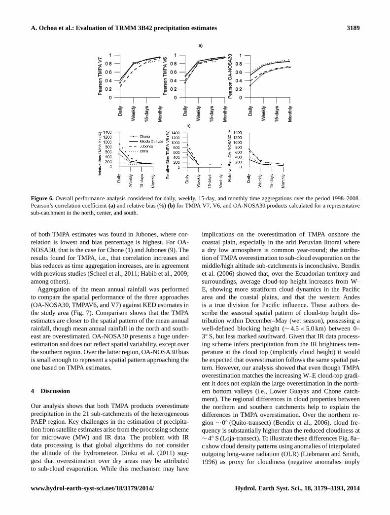
The Pearson correlation (Fig. 6a) and bias (Fig. 6b) were cal-culated on daily, weekly, 15-day, and monthly time scalesfor TMPAV7, V6, and OA-NOSA30. In general, correlationincreases with time scale, and is higher for monthly than 15-day and weekly time aggregated periods. Bias seems to accu-mulate when time aggregation increases, as found for WRFin other regions (Cheng and Steenburgh, 2005; Ruiz et al.,2010). The purpose of finding the relative bias in the esti-mates is to quantify respectively the over-/underestimationof the precipitation depth. The relative bias is consistent withthe correlation coefficient, decreasing as the time aggrega-tion increases. Although the daily bias is high in Jubones(9) (∼ 1000 % for V7 and∼ 1200 % for V6) and in MiddleGuayas (4) (higher for V7 than V6), on a weekly-to-monthlyscale the bias percentage decreases. The worst performance

Hydrol. Earth Syst. Sci., 18, 3179–3193, 2014 www.hydrol-earth-syst-sci.net/18/3179/2014/

A. Ochoa et al.: Evaluation of TRMM 3B42 precipitation estimates 3189

30

827

828

Figure 6. Overall performance analysis considered for daily, weekly, 15-daily and monthly time 829

aggregations over the period 1998-2008. a) Pearson's correlation coefficient and b) relative bias (%) 830

for TMPA V7, V6 and OANOSA-30 products calculated for a representative sub-catchment in the 831

north, centre and south. 832

833

Figure 7. Spatial distribution of mean annual precipitation over the period 1998-2008 according to the 834

KED interpolation of 98 rain gauges (a), OA-NOSA30 (b), TMPA V6 (c) and TMPA V7 (d). 835

Figure 6. Overall performance analysis considered for daily, weekly, 15-day, and monthly time aggregations over the period 1998–2008.Pearson’s correlation coefficient(a) and relative bias (%)(b) for TMPA V7, V6, and OA-NOSA30 products calculated for a representativesub-catchment in the north, center, and south.

of both TMPA estimates was found in Jubones, where cor-relation is lowest and bias percentage is highest. For OA-NOSA30, that is the case for Chone (1) and Jubones (9). Theresults found for TMPA, i.e., that correlation increases andbias reduces as time aggregation increases, are in agreementwith previous studies (Scheel et al., 2011; Habib et al., 2009;among others).

Aggregation of the mean annual rainfall was performedto compare the spatial performance of the three approaches(OA-NOSA30, TMPAV6, and V7) against KED estimates inthe study area (Fig. 7). Comparison shows that the TMPAestimates are closer to the spatial pattern of the mean annualrainfall, though mean annual rainfall in the north and south-east are overestimated. OA-NOSA30 presents a huge under-estimation and does not reflect spatial variability, except overthe southern region. Over the latter region, OA-NOSA30 biasis small enough to represent a spatial pattern approaching theone based on TMPA estimates.

4 Discussion

Our analysis shows that both TMPA products overestimateprecipitation in the 21 sub-catchments of the heterogeneousPAEP region. Key challenges in the estimation of precipita-tion from satellite estimates arise from the processing schemefor microwave (MW) and IR data. The problem with IRdata processing is that global algorithms do not considerthe altitude of the hydrometeor. Dinku et al. (2011) sug-gest that overestimation over dry areas may be attributedto sub-cloud evaporation. While this mechanism may have

implications on the overestimation of TMPA onshore thecoastal plain, especially in the arid Peruvian littoral wherea dry low atmosphere is common year-round; the attribu-tion of TMPA overestimation to sub-cloud evaporation on themiddle/high altitude sub-catchments is inconclusive. Bendixet al. (2006) showed that, over the Ecuadorian territory andsurroundings, average cloud-top height increases from W–E, showing more stratiform cloud dynamics in the Pacificarea and the coastal plains, and that the western Andesis a true division for Pacific influence. These authors de-scribe the seasonal spatial pattern of cloud-top height dis-tribution within December–May (wet season), possessing awell-defined blocking height (∼ 4.5< 5.0 km) between 0–3◦ S, but less marked southward. Given that IR data process-ing scheme infers precipitation from the IR brightness tem-perature at the cloud top (implicitly cloud height) it wouldbe expected that overestimation follows the same spatial pat-tern. However, our analysis showed that even though TMPAoverestimation matches the increasing W–E cloud-top gradi-ent it does not explain the large overestimation in the north-ern bottom valleys (i.e., Lower Guayas and Chone catch-ment). The regional differences in cloud properties betweenthe northern and southern catchments help to explain thedifferences in TMPA overestimation. Over the northern re-gion ∼ 0◦ (Quito-transect) (Bendix et al., 2006), cloud fre-quency is substantially higher than the reduced cloudiness at∼ 4◦ S (Loja-transect). To illustrate these differences Fig. 8a–c show cloud density patterns using anomalies of interpolatedoutgoing long-wave radiation (OLR) (Liebmann and Smith,1996) as proxy for cloudiness (negative anomalies imply

www.hydrol-earth-syst-sci.net/18/3179/2014/ Hydrol. Earth Syst. Sci., 18, 3179–3193, 2014

3190 A. Ochoa et al.: Evaluation of TRMM 3B42 precipitation estimates

Figure 7. Spatial distribution of mean annual precipitation over the period 1998–2008 according to the KED interpolation of 98 rain gauges(a), OA-NOSA30(b), TMPA V6 (c), and TMPA V7(d).

Figure 8. Monthly anomalies of OLR (Watts m−2) during 1998–2008 within the rainy season December–January (left), February–March(center), April–May (right).

increased cloudiness) during the rainy season within 1998–2008. During December–January (Fig. 8a) symmetrical pat-terns of cloudiness are observed over northern and south-ern sub-catchments, followed by increased cloudiness whichconcentrates over the northwestern edge during January–February (Fig. 8b). Then, cloudiness exhibits a markednorth–southeast gradient in April–May (Fig. 8c). This sug-gests that in addition to the error introduced by the estimationof the cloud-top, the TMPA overestimation for the northerncatchments may also be influenced by frequent occurrenceof low stratiform clouds (typical on the coastal area) whichunder stable conditions are detached from precipitation pat-terns (Bendix, et al., 2006). This high density of non-rainproducing clouds would affect the IR data retrieval resultingin overestimation.

The largest deficiencies of TMPA estimates are encoun-tered in separating the windward/leeward effect of the An-dean ridges on orographic rainfall which is particularly

witnessed in Jubones where the leeward effect is dominant.West of the climate divide there is no typical precipitationgradient. Through blocking at the ridges and through re-evaporation, rainfall of any origin more frequently affectshigher elevations than valley floors (Emck, 2007).

TMPA V7 and V6 estimates show different region-wideskills on a daily basis but they yield comparable resultsparticularly in the southern region (3.6–6◦ S) in weekly tomonthly time aggregations. TMPA V7 shows localized skillthat is higher than V6 on short-steep coastal and ocean-exposed sub-catchments but similar or lower skills on largeinland basins. The improvement is seen in the detection ca-pacity of light orographic precipitation on coastal ocean-exposed sub-catchments, where the spatial sampling seemsto capture small precipitation gradients. Over coastal areas,the orographic enhancement is a small spatial-scale event(Minder et al., 2008, Cheng et al., 2013). In the innermostsub-catchments where gradients of annual precipitation may

Hydrol. Earth Syst. Sci., 18, 3179–3193, 2014 www.hydrol-earth-syst-sci.net/18/3179/2014/

A. Ochoa et al.: Evaluation of TRMM 3B42 precipitation estimates 3191

reach 700 mm/100 m at 3400 m a.s.l. (Emck, 2007) the tem-poral sampling of V7 cannot capture the rapid evolution oforographic rainfall and the overestimation is similar to that ofthe V6 version. Notice that inland the total residual varianceand the KED uncertainty increase with elevation (especiallyfor V6). This could influence the apparent decrease of theV6 performance seen for the innermost sub-catchments. Thisis, however, restricted to very few sub-catchments where thespatial average is dominated by the weight of high altitudestations.

OA-NOSA30 product only shows reasonable skills in thesouthern region (3.6–6◦ S) where amount and occurrenceare relatively well represented. The greatest NWP limita-tions are encountered in representing the fast enhancementof rain rates due to the effect of the coastal mountains as afirst barrier for moisture transport in short-steep coastal sub-catchments (3–3.6◦ S). The nearly null NWP detection ca-pability is likely related to the unique rainfall rates that oc-cur on the ocean facing foothills of the Cordillera Costan-era. Unlike in most tropical mountains where convectiverainfall dominates, in southeast Ecuador vigorous advectionshapes a monotonic increasing precipitation gradient withaltitude. In the core of the southern region, Emck (2007)reported that rainfall originates from an equal balance ofadvective–topographic (light) and convective (heavier) gen-esis. Such a characteristic, over the southern region, sug-gests that the NWP parameterization for OA-NOSA30 is par-ticularly suited to solve for this type of precipitation. Forthe northern regions, which are more affected by the an-nual movement of the ITCZ, the influence of the continentalclimate divide and the occurrence of more stratiform cloud,deep convection (likely the dominant mechanism) is not em-ulated by the NWP model. A complete description of the er-rors in the NWP implementation is out of the scope of thisstudy; we therefore only highlight some of the major sources.The lateral boundary conditions (reanalysis data set) havepresumably a major role on the degradation of WRF productquality. The poor representation of the Andes in the reanal-ysis model has been shown to contribute to a modest simu-lation of meteorological fields such as wind (Schafer et al.,2003). Maussion et al. (2011) found that some undesired nu-merical effects and, eventually, inadequate input data can af-fect the operational output of the WRF model, in particularfor extreme events; that is probably by overstressing certainphysical processes. Jankov et al. (2005) found that the great-est variability in rainfall estimates from the WRF model orig-inates from changes in the choice of the convective scheme,although notable impacts were observed from changes in themicrophysics and planetary boundary layer (PBL) schemes.However, Ruiz et al. (2010) found that rainfall estimatesonly vary slightly among different configurations, but biasesincrease with time aggregation. Those findings agree withprevious studies (Blázquez and Nuñez, 2009; Pessacg, 2008)and suggest that there is a common deficiency in the convec-tive schemes used for this model.

5 Conclusions

In general, TRMM V7, V6, and OA-NOSA30 estimatescapture the most prominent seasonal features of precipita-tion in the study area. Quantitatively, only the southern sub-catchments of Ecuador and northern Peru are well estimatedby both satellite and NWP estimates. There is low accu-racy of both approaches in the northern and central regionswhere TMPA V7 and V6 overestimate precipitation whileOA-NOSA30 systematically underestimates. The improve-ment of V7 over V6 is not evident region wide. It appearsthat V7 detects better light precipitation rates on coastal andocean-exposed basins. Inland the differences of the two ver-sions of TRMM 3B42 are almost unnoticeable. The separa-tion of the windward/leeward Andean effect on orographicprecipitation appears the main challenge for TMPA algo-rithms. It was found that the detection probability is bet-ter for small rainfall depths (less than 5 mm day−1) than forhigh amounts of precipitation. OA-NOSA30 showed the bestskills in detecting a balanced advective/convective regime ofprecipitation in the southern region.

Analysis of daily, weekly, 15-day, and monthly time se-ries revealed that the correlation with station observationsincreases and bias decreases with the time aggregation. Dif-ferences are considerably larger for daily than weekly ag-gregation. The correlation and bias values are similar in thenorthern and southern region but in the central region corre-lation is smaller and bias is higher for all time aggregations.TMPA V7, V6, and OA-NOSA30 are able to capture rela-tively well the spatial pattern in the southern region of thestudy area, but the performance of both approaches reducesin the northern and central region. In general the two TMPAversions perform better than OA-NOSA30.

In view of hydrological and water resources managementapplications, it has been demonstrated that the potential in-take of both satellite and NWP estimates in the PAEP regiondiffers among catchments and precipitation regimes. Ouranalysis has shown that both approaches capture the meanspatial and temporal features of precipitation at weekly tomonthly accumulations over a particular region of southernEcuador and northern Peru. These findings are relevant forthese poorly gauged regions where there is growing pool ofmodeling work that relies on the use of satellite-based rain-fall estimates as forcing data. Also dynamical weather pre-diction becomes more frequently applied, but this predictionis still in an experimental stage. However, for operational ap-plications such as flood warnings, which demand high tem-poral resolution rainfall data, accurate depth and storm lo-cation estimates are mandatory. The usefulness of both esti-mates is less promising.

www.hydrol-earth-syst-sci.net/18/3179/2014/ Hydrol. Earth Syst. Sci., 18, 3179–3193, 2014

3192 A. Ochoa et al.: Evaluation of TRMM 3B42 precipitation estimates

Acknowledgements.L. Pineda was funded by an EMECW grantof the European Commission for doctoral studies at KU Leuven.A. Ochoa acknowledges VLIR-UOS for a scholarship, whichenabled a study stay in Belgium. Gratitude is expressed to thenational meteorology and hydrology services of Ecuador (R. Mejía,INAMHI) and Peru (H. Yauri, SENAMHI) for making the stationdata available. The authors thank D. Mora (PROMAS-CuencaUniversity) for assistance with geospatial information.

Edited by: W. Buytaert

References

Arias-Hidalgo, M., Bhattacharya, B., Mynett, A. E., andvan Griensven, A.: Experiences in using the TMPA-3B42R satel-lite data to complement rain gauge measurements in the Ecuado-rian coastal foothills, Hydrol. Earth Syst. Sci., 17, 2905–2915,doi:10.5194/hess-17-2905-2013, 2013.

Becker, A., Finger, P., Meyer-Christoffer, A., Rudolf, B.,Schamm, K., Schneider, U., and Ziese, M.: A description of theglobal land-surface precipitation data products of the Global Pre-cipitation Climatology Centre with sample applications includ-ing centennial (trend) analysis from 1901–present, Earth Syst.Sci. Data, 5, 71–99, doi:10.5194/essd-5-71-2013, 2013.

Bendix, J. and Bendix, A.: Climatological Aspects of the 1991/1993El Niño in Ecuador, Bulletin de L’Institut Francaise d’EtudesAndines., 27, 655–666,http://lcrs.geographie.uni-marburg.de/fileadmin/media_lcrs/paper_bendix/BENDIX_BIFED98.PDF(last access: 12 December 2013), 1998.

Bendix, A. and Bendix, J.: Heavy rainfall episodes in Ecuadorduring El Niño events and associated regional atmosphericcirculation and SST patterns, Adv. Geosci., 6, 43–49,doi:10.5194/adgeo-6-43-2006, 2006.

Bendix, J., Rollenbeck, R., Gottlicher, D., and Cermank, J.: Cloudocurrence and cloud properties in Ecuador, Clim. Res., 30, 133–147, 2006.

Bendix, J., Trachte, K., Palacios, E., Rollenbeck, R., Göttlicher, D.,Nauss, T., and Bendix, A.: El Niño meets La Niña-Anomalousrainfall patterns in the “Traditional” El Niño region of southernEcuador, Erdkunde, 65, 151–167, 2011.

Blázquez, J. and Nuñez, M. N.: Sensitivity to convective parameter-ization in the WRF regional model in southern South America,in: Ninth Int. Conf. on Southern Hemisphere Meteorology and,Oceanography, Melbourne, Australia., p. 6, Amer. Meteor. Soc.,2009.

Buytaert, W., Celleri, R., Willems, P., De Bièvre, B., and Wyseure,G.: Spatial and temporal rainfall variability in mountainous ar-eas: A case study from the south Ecuadorian Andes, J. Hydrol.,329, 413–421, doi:10.1016/j.jhydrol.2006.02.031, 2006.

Cedeño, J. and Cornejo, M. P.: Evaluation of three pre-cipitation products on ecuadorian coast, available at:http://wcrp.ipsl.jussieu.fr/Workshops/Reanalysis2008/Documents/Posters/P3-25_ea.pdf(last access: 12 April 2012),2008.

Chen, Y., Ebert, E. E., Walsh, K. J. E., and Davidson, N. E. : Eval-uation of TRMM 3B42 precipitation estimates of tropical cy-clone rainfall using PACRAIN data, J. Geophys. Res. Atmos.,118, 2184–2196, doi:10.1002/jgrd.50250, 2013.

Cheng, W. Y. Y. and Steenburgh, W. J.: Evaluation of SurfaceSensible Weather Forecasts by the WRF and the Eta Modelsover the Western United States, Weather Forecast., 20, 812–821,doi:10.1175/WAF885.1, 2005.

Dinku, T., Ruiz, F., Connor, S. J., and Ceccato, P.: Vali-dation and Intercomparison of Satellite Rainfall Estimatesover Colombia, J. Appl. Meteorol. Climatol., 49, 1004–1014,doi:10.1175/2009JAMC2260.1, 2010.

Dinku, T., Ceccato, P., and Connor, S. J.: Challenges ofsatellite rainfall estimatin over 626 mountainous and aridparts of east Africa, Int. J. Remote Sens., 30, 5965–5979,doi:10.1080/01431161.2010.499381, 2011.

Emck, P.: A climatology of South Ecuador, Unpublished PhD The-sis. Universität 631 Erlangen, Germany, 2007.

Habib, E., Henschke, A., and Adler, R. F.: Evaluation of TMPAsatellite-based research and real-time rainfall estimates duringsix tropical-related heavy rainfall events over Louisiana, USA,Atmos. Res., 94, 373–388, doi:10.1016/j.atmosres.2009.06.015,2009.

Haylock, M. R., Hofstra, N., Klein Tank, A. M. G., Klok,E. J., Jones, P. D., and New, M.: A European daily high-resolution gridded data set of surface temperature and pre-cipitation for 1950–2006, J. Geophys. Res., 113, D20119,doi:10.1029/2008JD010201, 2008.

Huffman, G. J. and Bolvin, D. T.: TRMM and other data precip-itation data set documentation, Global Change Master Direc-tory, NASA, 40 pp., available at:ftp://precip.gsfc.nasa.gov/pub/trmmdocs/3B42_3B43_doc.pdf, last access: 15 May 2014.

Huffman, G. J., Adler, R. F., Bolvin, D. T., Gu, G., Nelkin,E. J., Bowman, K. P., Hong, Y., Stocker, E. F., andWolff, D. B.: The TRMM Multisatellite Precipitation Analy-sis (TMPA): Quasi-Global, Multiyear, Combined-Sensor Precip-itation Estimates at Fine Scales, J. Hydrometeorol, 8, 38–55,doi:10.1175/JHM560.1, 2007.

Huffman, G. J., Adler, R. F., Bolvin, D. T., and Nelkin, E. J.: TheTRMM multi-satellite precipitation analysis (TMPA), in: Satel-lite Rainfall Applications for Surface Hydrology, edited by: Ge-bremichael, M. and Hossain, F., Springer Science, New York,USA, 2010.

Jankov, I., Jr., W. A. G., Segal, M., Shaw, B. and Koch, S. E.: TheImpact of Different WRF Model Physical Parameterizations andTheir Interactions on Warm Season MCS Rainfall, Weather Fore-cast., 20, 1048–1060, doi:10.1175/WAF888.1, 2005.

Kistler, R., Kalnay, E., Collins, W., Saha, S., White, G., Woollen,J., Chelliah, M., Ebisuzaki, W., Kanamitsu, M., Kousky, V., VanDen Dool, H., Jenne, R., and Fiorino, M.: The NCEP-NCAR 50-year reanalysis: monthly means CD-ROM and documentation,Bull. Am. Meteorol. Soc., 82, 247–267, 2001.

Li, J. and Heap, A. D.: A Review of Spatial Interpolation Meth-ods for Environmental Scientists, Geoscience Australia, 200,137, available at:http://www.ga.gov.au/image_cache/GA12526.pdf (last access: 17 July 2012), 2008.

Liebmann, B. and Smith, C. A.: Description of a Complete (Interpo-lated) Outgoing Longwave Radiation Dataset, Bull. Amer. Me-teor. Soc., 77, 1275–1277, 1996.

Maussion, F., Scherer, D., Finkelnburg, R., Richters, J., Yang, W.,and Yao, T.: WRF simulation of a precipitation event over theTibetan Plateau, China – an assessment using remote sensing and

Hydrol. Earth Syst. Sci., 18, 3179–3193, 2014 www.hydrol-earth-syst-sci.net/18/3179/2014/

A. Ochoa et al.: Evaluation of TRMM 3B42 precipitation estimates 3193

ground observations, Hydrol. Earth Syst. Sci., 15, 1795–1817,doi:10.5194/hess-15-1795-2011, 2011.

Minder, J. R., Durran, D. R., Roe, G. H., and Anders, A. M.:The climatology of small-scale orographic precipitation over theOlympic Mountains: Patterns and processes, Q. J. R. Meteorol.Soc., 134, 817–839, 2008.

Muñoz, Á, G. and Recalde, C.: OA_NOSA30 dataset, available at:http://iridl.ldeo.columbia.edu/SOURCES/.U_Zulia/.CMC/.OA_NOSA30/.surface/(last access: 3 May 2012), 2010.

Muñoz, A., Lopez, P., Velasquez, R., Monterrey, L., Leon, G., Ruiz,F., Recalde, C., Cadena, J., Mejia, R., Paredes, M., Bazo, J.,Reyes, C., Carrasco, G., Castellon, Y., Villarroel, C., Quintana,J., and Urdaneta, A.: An Environmental Watch System for theAndean countries: El Observatorio Andino, Bull. Amer. Meteor.Soc., 91, 1645–1652, doi:10.1175/2010BAMS2958.1, 2010.

Pebesma, E.: CRAN – Package gstat, available at:http://cran.r-project.org/web/packages/gstat/index.html(last access: 17 July2012), 2011.

Pessacg, N.: Precipitation sensitivity experiments using WRF, 80pp., University of Buenos Aires, Argentina, 2008 (in Spanish).

Pineda, L., Ntegeka, V., and Willems, P.: Rainfall variabilityrelated to sea surface temperature anomalies in a Pacific–Andean basin into Ecuador and Peru, Adv. Geosci., 33, 53–62,doi:10.5194/adgeo-33-53-2013, 2013.

Romilly, T. G. and Gebremichael, M.: Evaluation of satellite rainfallestimates over Ethiopian river basins, Hydrol. Earth Syst. Sci.,15, 1505–1514, doi:10.5194/hess-15-1505-2011, 2011.

Rossel, F. and Cadier, E.: El Nino and prediction of anomalousmonthly rainfalls in Ecuador, Hydrol. Process., 23, 3253–3260,doi:10.1002/hyp.7401, 2009.

Rossel, F., Le Goulven, P., and Cadier, E.: Areal distribution of theinfluence of ENSO on the annual rainfall in Ecuador, Revue desSciences de l’Eau, v. 12, 1999.

Ruiz, J. J., Saulo, C., and Nogués-Paegle, J.: WRF Model Sensitiv-ity to Choice of Parameterization over South America: Validationagainst Surface Variables, Mon. Weather Rev., 138, 3342–3355,doi:10.1175/2010MWR3358.1, 2010.

Schaefer, J. T.: The Critical Success Index as an Indicator of Warn-ing Skill, Weather Forecast., 5, 570–575, doi:10.1175/1520-0434(1990)005253C0570:TCSIAA253E2.0.CO;2, 1990.

Schafer, R., Avery, S. K., and Gage, K. S.: A comparison of VHFwind profiler observations 685 and the NCEP-NCAR Reanalysisover the tropical Pacific, J. App. Meteor., 42, 873–889, 2003.

Scheel, M. L. M., Rohrer, M., Huggel, Ch., Santos Villar, D., Sil-vestre, E., and Huffman, G. J.: Evaluation of TRMM Multi-satellite Precipitation Analysis (TMPA) performance in the Cen-tral Andes region and its dependency on spatial and tem-poral resolution, Hydrol. Earth Syst. Sci., 15, 2649–2663,doi:10.5194/hess-15-2649-2011, 2011.

Skamarock, W. C., Klemp, J. B., Dudhia, J., Gill, D. O., Barker, D.M., Wang, W., and Powers, J. G.: A Description of the AdvancedResearch WRF Version 2. NCAR Tech note., 2005.

Su, F., Hong, Y., and Lettenmaier, D. P.: Evaluation of TRMM Mul-tisatellite Precipitation Analysis (TMPA) and Its Utility in Hy-drologic Prediction in the La Plata Basin, J. Hydrometeorol., 9,622–640, doi:10.1175/2007JHM944.1, 2008.

Wang, X., Chen, H., and Wu, Y.: New techniques for thedetection and adjustment of shifts in daily precipitationdata series, J. Appl. Meteorol. Climatol., 49, 2416–2436,doi:10.1175/2010JAMC2376.1, 2010.

Wang, X. L. and Feng, Y.: Software for detection and adjustmentof shifts in daily precipitation data series, available at:http://etccdi.pacificclimate.org/software.shtml(last access: 17 July2012), 2012.

Ward, E., Buytaert, W., Peaver, L., and Wheater, H.: Evaluation ofprecipitation products over complex mountainous terrain: A wa-ter resources perspective, Adv. Water Resour., 34, 1222–1231,doi:10.1016/j.advwatres.2011.05.007, 2011.

Willems, P.: Quantification and relative comparison of differenttypes of uncertainties in sewer water quality modelling, WaterResearch, 42, 3539–3551, 2008.

Willems, P.: Model uncertainty analysis by variance decomposition,Phys. Chem. Earth, 42–44, 21–30, 2012.

Wilson, E. M.: Engineering Hydrology, 3rd Edn., Macmillan., 1983.Yamamoto, J. K.: An alternative measure of the reliability

of ordinary kriging estimates, Math. Geol., 32, 489–509,doi:10.1023/A:1007577916868, 2000.

Zulkafli, Z., Buytaert, W., Onof, C., Manz, B., Tarnavsky, E.,Lavado, W., and Guyot, J.: A comparative performance analy-sis of TRMM 3B42 (TMPA) versions 6 and 7 for hydrologicalapplications over Andean-Amazon river basins, J. Hydrometeor.,15, 581–592, doi:10.1175/JHM-D-13-094.1, 2014.

www.hydrol-earth-syst-sci.net/18/3179/2014/ Hydrol. Earth Syst. Sci., 18, 3179–3193, 2014