Evaluation of the State-of-the-Art Contaminated Sediment

Transport and Fate Modeling System

R E S E A R C H A N D D E V E L O P M E N T

EPA/600/R-06/108 September 2006

Evaluation of the State-of-the-Art Contaminated Sediment Transport and Fate Modeling System

by

Earl J. Hayter Ecosystems Research Division

National Exposure Research Laboratory Athens, GA 30605

U.S. Environmental Protection Agency Office of Research and Development

Washington, DC 20460

NOTICE

The information in this document has been funded by the United States Environmental Protection Agency. It has been subjected to the Agency=s peer and administrative review, and it has been approved for publication as an EPA document. Mention of trade names of commercial products does not constitute endorsement or recommendation for use.

ABSTRACT

Modeling approaches for evaluating the transport and fate of sediment and associated contaminants are briefly reviewed. The main emphasis is on: 1) the application of EFDC (Environmental Fluid Dynamics Code), the state-of-the-art contaminated sediment transport and fate public domain modeling system, to a 19-mile reach of the Housatonic River, MA; and 2) the evaluation of a 15-year simulation of sediment and PCB transport and fate in this 19-mile reach. The development of EFDC has been supported by Regions 1 and 4, the Office of Water, the Office of Superfund Remediation Technology Innovation (OSRTI), and the Office of Research and Development (ORD) - NERL/ERD. EFDC is currently being used at the following Superfund sites: Housatonic River, MA; Kalamazoo River, MI; Lower Duwamish Waterway, WA; and Portland Harbor, OR.

The evaluation of the modeling results showed that EFDC is capable of simulating the transport and resultant concentrations of TSS and PCBs in this reach of the Housatonic River within specified model performance measures. Specifically, a statistical summary of the performance of the EFDC model for TSS and PCB concentrations found that the relative bias at the downstream boundary of the model domain (i.e., Rising Pond dam) is well within the model performance measure of ± 30% for TSS (-11.93%) and just outside the measure for PCB concentrations (-31.97%). For median relative error, the model performance measure is also ± 30%, and the EFDC model is within the performance measure for both TSS (-27.12%) and PCB (-3.32%) concentrations. Considering the fact that the model was only minimally calibrated, and that the system modeled had widely varying hydraulic and morphologic regimes, the EFDC model's performance, as quantified by relative bias and median relative errors, is considered good. This demonstrates that EFDC is a robust modeling system that can be successfully implemented at other contaminated sediment sites.

ii

CONTENTS Page No.

Abstract ...................................................................................................................................... ii

Figures.........................................................................................................................................v

Tables ...................................................................................................................................... viii

Acronyms .................................................................................................................................. ix

1 Introduction.....................................................................................................................1 1.1 Background .........................................................................................................1 1.2 Components of contaminated sediment transport modeling study .....................2 1.3 Purpose and scope of model evaluation..............................................................5 1.4 Organization of report .........................................................................................6

2 Description of EFDC ....................................................................................................11 2.1 Description of Model ........................................................................................11 2.2 Hydrodynamics and Transport Model ..............................................................12 2.3 Sediment Transport Model................................................................................16

2.3.1 Non-cohesive sediment transport processes ............................................17 2.3.2 Cohesive sediment transport processes....................................................18

2.4 Contaminant Transport and Fate Model ...........................................................19

3 Model Application .......................................................................................................22 3.1 Overview...........................................................................................................22 3.2 Spatial Domain..................................................................................................22 3.3 Model Grid........................................................................................................23 3.4 Model Inputs .....................................................................................................23

3.4.1 Geometry, floodplain topography, and river bathymetry ........................24 3.4.2 Bottom friction and vegetative resistance in the riverbed and

floodplain.................................................................................................24 3.4.3 Sediment bed and floodplain soil composition and PCB

Concentrations.........................................................................................25 3.4.4 Hydraulic characteristics of the four dams ..............................................27 3.4.5 Initial conditions ......................................................................................28 3.4.6 Boundary conditions ................................................................................28

3.5 Model Parameters .............................................................................................29 3.5.1 Partitioning of PCBs in pore water and the water column.......................29 3.5.2 Sediment – water column PCB exchange ................................................30 3.5.3 Sediment Particle Mixing.........................................................................30 3.5.4 Volatilization............................................................................................30

4 Model Evaluation..........................................................................................................59

iii

5

4.1 Model Application ............................................................................................59 4.2 Model-Data Comparisons for Water Column TSS and PCBs ..........................59 4.3 Model Results for Sediment PCB Concentrations............................................60 4.4 Evaluation of Model Performance ....................................................................61 4.5 Process-Based Flux Summaries ........................................................................62

Conclusion ....................................................................................................................82

References .................................................................................................................................83

Glossary ....................................................................................................................................93

Appendices

A Sediment Properties and Transport ...............................................................................98

B Sediment Gradation Scale ...........................................................................................127

iv

FIGURES

Fig. No. Page No.

1.1 Sample CSM for Sediment Site (after USEPA, 2005)....................................................8

1.2 Housatonic River Watershed (after WESTON, 2006)....................................................9

1.3 Housatonic River Reaches 5 through 8 (after WESTON, 2006) ..................................10

3.1 Housatonic River Reaches 5 through 8 (after WESTON, 2006) ..................................33

3.2 Housatonic River between Woods Pond and Great Barrington (after WESTON, 2006) .................................................................................................34

3.3 Spatial Domain of the EFDC Model Showing Variation in Bottom Elevation (in meters – NAD 83 (86)) (after WESTON, 2006) ........................35

3.4a Foodchain Reaches 7a – 7e from Woods Pond Dam to Willow Mill Dam(after WESTON, 2006) .................................................................................................36

3.4b Foodchain Reaches 7f – 8 from Willow Mill Dam to Rising Pond Dam(after WESTON, 2006) .................................................................................................37

3.5a Longitudinal Bottom Gradient Profile Showing Foodchain Reaches 7A – 8 (after WESTON, 2006) .................................................................................................38

3.5b Longitudinal Bottom Gradient Profile in Reaches 7 and 8 Showing Location of the Four Dams (after WESTON, 2006) ....................................................................38

3.6a Computation grid for EFDC model – upstream boundary is at the top of this figure ......................................................................................................................39

3.6b Computation grid for EFDC model – lateral black line in the middle of this stretch is Columbia Mill dam (arrow points to dam) ....................................................40

3.6c Computation grid for EFDC model...............................................................................41

3.6d Computation grid for EFDC model...............................................................................42

3.6e Computation grid for EFDC model...............................................................................43

3.6.f Computation grid for EFDC model – lateral black line in the left third of this v

stretch is Willow Mill dam (arrow points to dam)........................................................44

3.6.g Computation grid for EFDC model – lateral black line on the right hand side (i.e., upstream end) of this stretch is Willow Mill dam ................................................45

3.6.h Computation grid for EFDC model – Stockbridge golf course is in the middle of this stretch.................................................................................................................46

3.6.i Computation grid for EFDC model – lateral black line in the middle of this stretch (immediately to the left – or downstream – of the red colored cells) is Glendale dam (arrow points to dam).............................................................................47

3.6.j Computation grid for EFDC model – lateral black line in the upper right corner of this figure is Glendale dam.......................................................................................48

3.6.k Computation grid for EFDC model – the downstream end of this figure is the upper part of Rising Pond .............................................................................................49

3.6.l Computation grid for EFDC model – the downstream end of this figure is Rising Pond (arrow points to Rising Pond dam)...........................................................50

3.7a Photo of Stockbridge golf course..................................................................................51

3.7b Grid in the area of the Stockbridge golf course ............................................................52

3.8 Initial Longitudinal Distributions of Grain Sizes for the River Bed Sediment.............53

3.9 Initial Longitudinal Distributions of Bulk Densities for the River Bed Sediment .......54

3.10 Initial Longitudinal Distributions of Porosities for the River Bed Sediment ...............55

3.11 Initial Longitudinal Distributions of Sediment Bed PCB Concentrations for the River Bed Sediment...........................................................................................56

3.12 Initial Longitudinal Distributions of Fractions of Organic Carbon for the River Bed Sediment...........................................................................................57

3.13 Initial OC-Normalized PCB Concentrations (Segregated into 1-Mile Bins) versus River Mile (after WESTON, 2006) ...................................................................58

4.1a Comparison of Simulated (Solid Line) and Measured (Red Symbols) TSS and tPCB Concentrations in the Water Column for 1994-1995. DL = detection limit 67

4.1b Comparison of Simulated (Solid Line) and Measured (Red Symbols) TSS and tPCB Concentrations in the Water Column for 1996-1997. DL = detection limit.68

4.1c Comparison of Simulated (Solid Line) and Measured (Red Symbols) TSS

vi

and tPCB Concentrations in the Water Column for 1998-1999. DL = detection limit.69

4.1d Comparison of Simulated (Solid Line) and Measured (Red Symbols) TSS and tPCB Concentrations in the Water Column for 2000-2001. DL = detection limit.70

4.1e Comparison of Simulated (Solid Line) and Measured (Red Symbols) TSS and tPCB Concentrations in the Water Column for 2002-2003. DL = detection limit.71

4.1f Comparison of Simulated (Solid Line) and Measured (Red Symbols) TSS and tPCB Concentrations in the Water Column for 2004. DL = detection limit ..........72

4.2 Comparison of Simulated (Solid Line) and Measured (Red Symbols) TSS and tPCB Concentrations in the Water Column for April – June 1997. DL = detection limit ......................................................................................................73

4.3 Comparison of Simulated (Solid Line) and Measured (Red Symbols) TSS and tPCB Concentrations in the Water Column for July – September 2004. DL = detection limit ......................................................................................................74

4.4 Temporal Trend of tPCB Concentrations in Surface Sediments for Foodchain Reaches .......................................................................................................75

4.5 Cross-Plot of Simulated and Measured TSS.................................................................76

4.6 Cross-Plot of Simulated and Measured tPCB Concentrations......................................77

4.7 Probability Distributions of Simulated and Measured TSS Concentrations.................78

4.8 Probability Distributions of Simulated and Measured tPCB Concentrations...............79

4.9 Process-Based Annual Average Mass Flux Summary for Solids .................................80

4.10 Process-Based Annual Average Mass Flux Summary for PCBs..................................81

vii

TABLES

Table No. Page No.

1.1 Typical Elements of a CSM for a Contaminated Sediment Site (after USEPA, 2005) .......................................................................................................7

3.1 Effective Diameters for Non-Cohesive Sediment Classes............................................32

4.1 Statistical Evaluation of EFDC Model Performance, January 1994 – December 2004....................................................................................64

4.2 Process-Based Annual Average Mass Flux Summary Tabulation for Solids...............65

4.3 Process-Based Annual Average Mass Flux Summary Tabulation for PCBs................66

viii

ACRONYMS CEC Cation Exchange Capacity COC Chemical of Concern CSM Conceptual Site Model DOC Dissolved Organic Carbon EFDC Environmental Fluid Dynamic Code FCM Foodchain Model HSPF Hydrologic Simulation Program FORTRAN NERL National Exposure Research Laboratory PCB Polychlorinated Biphenyls PSA Primary Study Area (Reaches 5 and 6) SAR Sodium Adsorption Ratio SSC Suspended Sediment Concentration TOC Total Organic Carbon tPCB total PCBs TSS Total Suspended Solids USCOE U.S. Corps of Engineers USEPA U.S. Environmental Protection Agency USGS U.S. Geological Survey

ix

1 INTRODUCTION

1.1 Background

Remediation of bodies of water such as rivers, reservoirs, lakes, harbors and estuaries contaminated with PCBs, metals, metalloids, and other toxic chemicals is usually extremely expensive. The assessment and prediction of the transport and fate of contaminated sediments, and the associated chemical bioaccumulation are often key issues for both human and ecological risk assessments and remedial decision-making at Superfund sites, and the need for transparent and consistent approaches to this issue across sites and across Regions is self evident. Modeling the transport and fate of sediments and their adsorbed contaminants is often one of the tools used to assess remediation alternatives. Advanced numerical models that simulate the transport and fate of contaminants in surface waters are important tasks with which one can understand the complex physical, chemical and biological processes that govern contaminant transport and fate. However, no single assessment approach is appropriate for all sites, so there must also be flexibility in the rigor and scope of assessments while maintaining the consistency of principles.

The National Exposure Research Laboratory’s Ecosystem Research Division in Athens, GA has a research program entitled “Contaminated Sediment Transport and Fate Modeling”, the goal of which is to develop a consensus framework for transport/fate/bioaccumulation modeling at Superfund sites. This framework is to include modeling protocols for applying the component contaminated sediment transport and bioaccumulation models to evaluate proposed remediation measures at contaminated sediment Superfund sites. To accomplish this task, the following five research objectives are being performed:

1. Evaluation of existing contaminated sediment mass fate and transport models and adsorbed contaminant bioaccumulation models. Existing, public-domain contaminated sediment transport models were evaluated in 2003 (see Imhoff et al. 2003), and existing chemical bioaccumulation models were evaluated in 2004 (see Imhoff et al. 2004).

2. Testing of highest ranked contaminated sediment transport model. Based on the review performed by Imhoff et al. (2003), the highest ranked contaminated sediment transport model, EFDC (Environmental Fluid Dynamic Code), was subsequently tested in the following types of surface water bodies: river (Housatonic River, MA; reservoir (Lake Hartwell, GA/SC); salt-wedge estuary (Lower Duwamish Waterway, WA); and partially stratified estuary (St John-Ortega-Cedar Rivers, FL). The purpose of this testing was to evaluate the ability of EFDC to simulate the hydrodynamics, sediment transport and contaminant transport and fate in these different types of surface waters. In the Lower Duwamish Waterway, only the ability of EFDC to simulate the barotropic and baroclinic circulation in a salt-wedge estuary was evaluated (Arega and Hayter, 2006). In the St John-Ortega-Cedar Rivers, the ability of EFDC to simulate the hydrodynamics and sediment transport in a micro-tidal, partially stratified estuary was evaluated (Hayter et al., 2003). In both the Housatonic

1

River and Lake Hartwell, the ability of EFDC to simulate the hydrodynamics, sediment and contaminant transport and fate were evaluated.

3. Evaluation of EFDC by modeling the transport and fate of sediments and contaminants over a minimum of 10-years at a demonstration site. This evaluation is presented in this report and is discussed in Section 1.3.

4. Develop new modules for EFDC to address the identified sediment-related needs of OSRTI and the Regions. In 2003, OSRTI identified contaminated sediment-related research priorities that included the development of models to simulate processes such as the vertical transport of contaminants dissolved in the pore water of sediment out of the sediment and up through an overlying sediment cap. In response to these identified needs, algorithms to simulate the following processes have been (or are currently being) developed and incorporated into EFDC:

a) Simulation of consolidation due to sediment self-weight and cap-induced overburden, and the resulting upward flux of dissolved contaminants. This module has been completed and tested. A paper that will be submitted to a peer-reviewed journal is currently being prepared.

b) Simulation of wave-induced resuspension of highly organic sediments and the associated contaminants. This module is currently being developed under contract to the University of Florida.

c) Linking sediment transport, eutrophication and diagenesis modules in EFDC to account for resuspension and settling of inorganic sediment and organic matter. This work is to be performed by Tetra Tech under a Work Assignment starting in FY2007.

5. Develop a consensus framework for modeling remedial alternatives in surface waters. Building from the upgraded version of EFDC, a consensus framework for transport/fate and bioaccumulation modeling at contaminated sediment Superfund sites will be developed. This framework will include protocols for applying the component watershed loading model, the transport and fate modeling system, and the chemical bioaccumulation model.

1.2 Components of contaminated sediment transport modeling study

For the sake of completeness, the components of a complete and technically defensible contaminated sediment transport modeling study are briefly reviewed in this section. The reader should refer to EPA’s Contaminated Sediment Remediation Guidance for Hazardous Waste Sites (USEPA, 2005) for a more in-depth discussion of this topic.

Develop Conceptual Site Model: A conceptual site model (CSM) of a contaminated sediment site is a representation of an environmental system (e.g., watershed) and the physical, chemical, and biological processes that govern the transport of sediments and the transport, fate and transformation of contaminants from sources to receptors. Important elements of a CSM include information about both point and nonpoint

2

sediment and contaminant sources, transport pathways (both over land and in the water body), and exposure pathways (USEPA, 2005). Summarizing this information in one place helps in identifying data gaps and areas of uncertainty that might impact the subsequent remedial investigation (RI) and feasibility study (FS). The initial version of a CSM is usually a set of hypotheses derived from existing site data and possibility knowledge gained from other sites. The subsequent site investigation is a collection of field and laboratory studies conducted to test these hypotheses and quantify the qualitative descriptions in the initial CSM. The initial CSM is modified as additional source, pathway, and contaminant information is collected and analyzed during the site investigation. A thorough CSM along with a site tour are invaluable in determining whether or not a modeling study needs to be performed, and if so, what level of analysis/model is required. Typical elements of a CSM for a contaminated sediment site are listed in Table 1.1. An example schematization of a contaminated sediment CSM that focuses on sediment and contaminant transport and fate processes is shown in Figure 1.1.

Determine Whether a Modeling Study is Needed/Appropriate: The following questions (modified from USEPA, 2005) are useful, but not inclusive, for determining the appropriate use (if at all) of site-specific mathematical models:

• Are historical data and/or simple quantitative techniques available to determine the validity of the hypotheses in the CSM with the desired accuracy?

• Have the spatial extent, degree of heterogeneity, and levels of contamination at the site been defined?

• Have all significant ongoing sources of contamination been defined and their fluxes measured?

• Do sufficient data exist to support the use of a mathematical model, and if not, are time and resources available to collect the required data to achieve the desired level of confidence in model results?

• Are time and resources available to perform the modeling study itself?

In theory, the answers to the first three bullets should be given in the CSM. They are included here since the answers to these questions should be considered in addressing this issue. If the decision is made that some type of modeling is needed, the following material should be useful in deciding what type of model (or level of analysis) should be used.

Determine the Appropriate Level of Analysis: As in the previous step, the CSM should be consulted during this step. This step concerns determining if the most significant (i.e., first-order) processes and interactions that control the transport and/or fate of sediment and contaminants, as identified in the CSM, can be simulated with one or more existing contaminated sediment transport and fate models. If it is determined that there are existing models capable of simulating these governing processes, then the types of models (e.g., analytical, empirical, numerical) that have this capability should be identified. The model types that do not have this capability should not be used. If it is determined that there are no existing models capable of simulating, at a minimum, the most significant processes and interactions, then other tools or methods for evaluating proposed approaches should be identified and used. If it is determined that one or more models or types of mathematical models capable of

3

simulating the controlling transport and fate processes and interactions exist, then the process described previously should be used to choose the appropriate type of model. As shown in Imhoff et al. (2003), there are existing public domain numerical models that can simulate most of the physical, chemical and biological processes and interactions (e.g., those shown in Figure 1.1) that control the transport and fate of sediment and contaminants in water bodies, e.g., EFDC.

Choose the most appropriate model: If the decision is made to apply a numerical model at a contaminated sediment site, selection of the most appropriate contaminated sediment transport and fate model to use at a specific site is one of the critical steps in the modeling program. Familiarity with existing sediment and contaminant transport models is essential to perform this step. Comprehensive technical reviews of available sediment and contaminant transport and fate models and chemical bioaccumulation models have been conducted by the EPA’s ORD National Exposure Research Laboratory – please refer to Imhoff et al. (2003) and Imhoff et al. (2004).

Conduct a complete modeling study: Whenever numerical models are used, the following steps should be performed to yield a scientifically defensible modeling study: verification, calibration, validation, sensitivity analysis, and uncertainty analysis (the latter is not practical to perform with transport and fate models). These steps are discussed in the following:

Model verification: This step involves evaluation of 1) model theory, 2) consistency of the computer code with model theory, and 3) the computer code for integrity in the calculations. Model verification should be documented, or if the model is new, it should be peer-reviewed by an independent party. Whenever possible, public domain verified models, calibrated and validated to site-specific conditions should be used.

Model calibration: Uses site-specific information from a time period of record to adjust model parameters in the governing equations (e.g., bottom friction coefficient in hydrodynamic models) to obtain an optimal agreement between a measured data set and model calculations for the simulated state variables.

Model validation: Also referred to as model confirmation. This step consists of a demonstration that the calibrated model accurately reproduces known conditions over a different time period with the physical parameters and forcing functions changed to reflect the conditions during the new simulation period. The parameters adjusted during calibration should not be adjusted during validation. Model results from the validation simulation should be compared to the data set. If an acceptable level of agreement is achieved between the data and model simulations, then the model can be considered validated, at least for the range of conditions defined by the calibration and validation data sets. If an acceptable level of agreement is not achieved, then analysis should be performed to determine possible reasons for the differences between the model simulations and data. The latter sometimes leads to refinement of the model (e.g., using a finer model grid) or to the addition of one or more physical/chemical processes represented in the model.

4

Sensitivity analysis: This process consists of varying each of the input parameters by a fixed percent (while holding the other parameters constant) to determine how the model predictions vary. The resulting variations in simulated state variables are a measure of the sensitivity of model predictions to the parameter whose value was varied.

Uncertainty analysis: This process consists of propagating the relative error in each parameter (that was varied during the sensitivity analysis) to determine the resulting error in the model predictions. A probabilistic model, e.g., Monte Carlo Analysis, is one method of performing an uncertainty analysis. While quantitative uncertainty analyses are possible and practical to perform on watershed loading and food chain models, they are not so at present on transport and fate models. As a result, a thorough sensitivity analysis should be performed for the transport and fate models.

1.3 Purpose and scope of model evaluation

The purpose of this research is to evaluate the ability of EFDC, the state-of-the-art contaminated sediment modeling system, to simulate the transport and fate of a contaminant over a time period of at least 10 years. This time period was chosen since models would normally have to be run over a multi-decade time period to evaluate the effectiveness of various remedial measures, e.g., dredging, capping, dredging and capping, monitored natural recovery (MNR), in reducing the contaminant concentrations in both the sediment and water column. The demonstration site chosen was the Housatonic River in western Massachusetts. Specifically, a 19-mile reach of the Housatonic River immediately downstream of Woods Pond (see Figure 1.2) was chosen as the modeling domain. Reaches 5 through 8 of the Housatonic River are shown in Figure 1.3, and the 19-mile reach encompasses Reaches 7 and 8. Also shown in Figure 1.3 are Reaches 5 and 6; these reaches constitute the Primary Study Area (PSA), and were previously modeled by EPA Region 1 as described in the Modeling Framework Document (WESTON, 2004a), the Model Calibration Report (WESTON, 2004b), and the Model Validation Report (WESTON, 2006). For the purposes of this model evaluation, the same version of EFDC used by Region 1 was applied to Reaches 7 and 8. The application of EFDC to Reaches 7 and 8 is described in detail in Section 3.2. The strategy in applying EFDC to Reaches 7 and 8 was to test its performance in simulating the transport of sediment and PCBs over a multi-year period without the benefit of calibration or validation, thereby testing its robustness to yield satisfactory comparisons with data collected at a sampling station a short distance downstream of Reach 8, i.e., downstream of the downstream boundary of the modeling domain of Reaches 7 and 8. While the model was not calibrated or validated, hydrodynamic, sediment and PCB related parameterizations were changed in order to represent the vastly different hydraulic and morphologic regimes in Reaches 7 and 8 compared to those in the PSA. Especially considering the material presented in the previous section, it is important for the reader to understand that the model of Reaches 7 and 8 is in the traditional sense uncalibrated and unvalidated, and thus model results will naturally have a higher level of uncertainty associated with them than results obtained by a calibrated and validated model.

5

1.4 Organization of report

A description of EFDC is presented in Section 2, while a description of the application of EFDC to Reaches 7 and 8 is presented in Section 3. The evaluation of EFDC’s ability to simulate the transport of sediment and PCBs in these reaches is discussed in Section 4, and conclusions from this model evaluation study are presented in Section 5. In Appendix A, properties and transport processes of both cohesive and noncohesive sediments are described, while Appendix B contains a sediment gradation scale.

6

Table 1.1 Typical Elements of a CSM for a Contaminated Sediment Site (after USEPA, 2005)

Sources of contaminants of concern Exposure pathways for humans

• Upland soils • Fish/shellfish ingestion • Floodplain soils • Dermal uptake from wading, swimming • Surface water • Water ingestion • Groundwater • Inhalation of volatiles • Non-aqueous phase liquids (NAPL) and other source materials Exposure pathways for biota • Sediment “hot spots”

• Fish/shellfish/benthic invertebrate ingestion and storm water runoff outfalls • Outfalls, including combined sewer outfalls

• Incidental ingestion of sediment • Direct uptake from water • Atmospheric contaminants

Contaminant transport pathways Human receptors

• Sediment resuspension and deposition • Recreational fishers • Surface water transport • Subsistence fishers • Runoff • Waders/swimmers/birdwatchers • Bank erosion • Workers and transients • Groundwater advection • Bioturbation Ecological receptors • Molecular diffusion • Food chain • Benthic/epibenthic invertebrates

• Bottom-dwelling/pelagic fish • Mammals and birds (e.g., mink, otter, heron, bald eagle)

7

Figure 1.1 Sample CSM for Sediment Site (after USEPA, 2005)

8

Figure 1.2 Housatonic River Watershed (after WESTON, 2006)

9

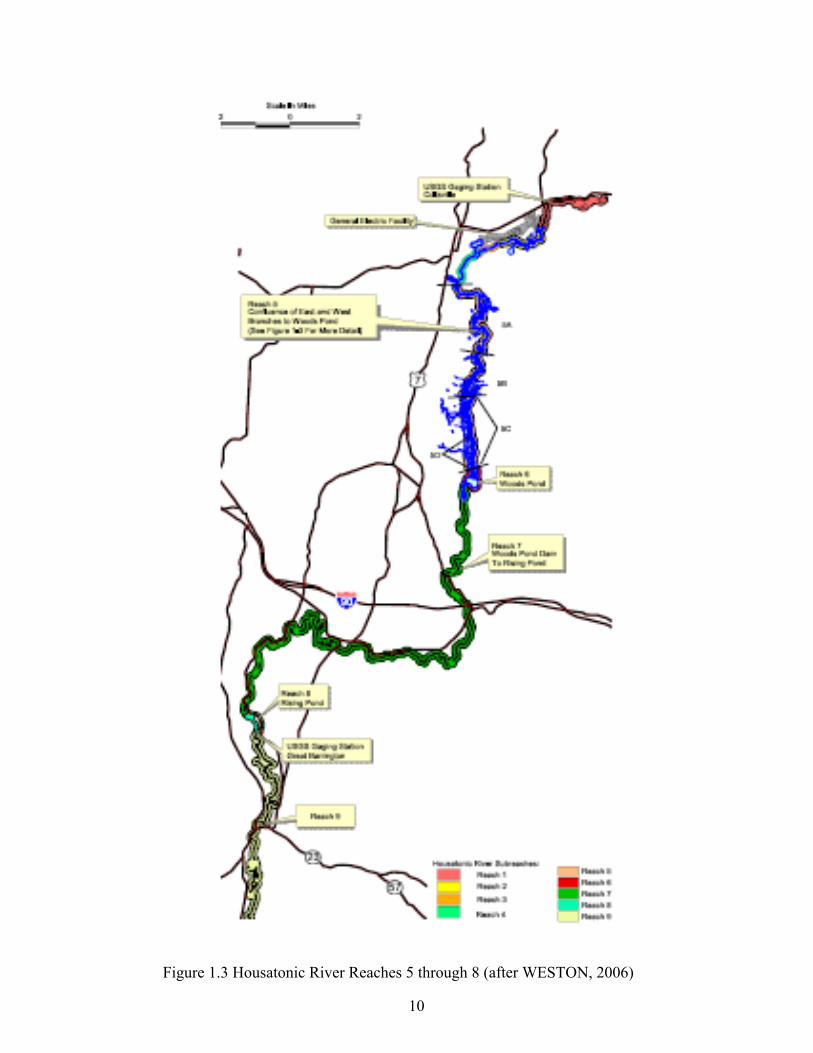
Figure 1.3 Housatonic River Reaches 5 through 8 (after WESTON, 2006)

10

2 DESCRIPTION of EFDC

2.1 Description of Model

As discussed in the previous section, the numerical model evaluated in this study was the Environmental Fluid Dynamics Code (EFDC) (Hamrick, 1992). Imhoff et al. (2003) evaluated public domain, contaminated sediment fate and transport models based on their numerical scheme, physical and chemical processes simulated, model support availability, and application history. EFDC was the top ranked model. EFDC is currently maintained by Tetra Tech, Inc. and supported by the U.S. EPA. EFDC is a three-dimensional (3D) public domain modeling system that has been widely used in water quality and contaminant transport studies. The application history of EFDC includes: simulating wetting and drying processes of the hydrodynamics and sediment transport in Morro Bay (Ji et al., 2000); thermal discharge study in Conowingo Pond (Hamrick and Mills, 2000); simulating Lake Okeechobee hydrodynamics, thermal, and sediment transport processes (Jin et al., 2002); studying tidal intrusion and its impact on larval dispersion in the James River estuary (Shen et al., 1999); modeling hydrodynamics and sediment transport in the middle Atlantic Bight (Kim et al., 1997); and modeling the hydrodynamics and water quality in Peconic Bay (Tetra Tech, 1999). EFDC has also been used to develop TMDLs in the following water bodies: Charles River, MA; Mashapaug Pond RI; Christiana River, DE and PA; Wissahickon Creek, PA; Cape Fear River, NC; Neuse River, NC; Jordon Lake, NC; Boone Reservoir, NC; Charleston Harbor, SC; Savannah River, GA; Brunswick Harbor, GA; Lake Allatoona, GA; Southern Four Basins, GA; St. Johns River, FL; Fenholloway River, FL; Myakka River Estuary, FL; Mobile Bay, AL; Ward Cover, AL; Alabama River, AL; Flint Creek, AL; Lake Jordon, AL; Lake Mitchell, AL; Logan Martin Lake, AL; Lay Lake, AL; Lake Neeley Henry, AL; Yazoo River, MS; Escatawpa River, MS; St. Louis Bay, MS; East Fork Little Miami River, OH; Ten Killer Ferry Lake, OK; Lake Wister, OK; Armanda Bayou, TX; Arroyo Colorado, TX; San Diego Bay, CA; Los Angeles River, CA; Los Angeles Harbor, CA; Big Bear Lake, CA; Canyon Creek, CA; Clear Lake, CA; a section of the Sacramento River, CA; and South Puget Sound, WA. As stated previously, EFDC is also currently being used at the following Superfund sites: Housatonic River, MA; Kalamazoo River, MI; Lower Duwamish Waterway, WA; and Portland Harbor, OR.

The EFDC model is a public domain, surface water modeling system incorporating fully integrated hydrodynamics. It solves the 3D, vertically hydrostatic, free surface, turbulence averaged equations of motion. EFDC is extremely versatile, and can be used for 1D, 2D-laterally averaged (2DV), 2D-vertically averaged (2DH), or 3D simulations of rivers, lakes, reservoirs, estuaries, coastal seas, and wetlands.

For realistic representation of horizontal boundaries, the governing equations are formulated such that the horizontal coordinates, x and y, are curvilinear. To provide uniform resolution in the vertical direction, the sigma (stretching) transformation is used. The equations of motion and transport solved in EFDC are turbulence-averaged, because prior to averaging, although they represent a closed set of instantaneous velocities and concentrations, they cannot be solved for turbulent flows. A statistical approach is applied, where the instantaneous values are decomposed into mean and fluctuating values to enable the solution. Additional terms that

11

represent the turbulence terms are introduced to the equations for the mean flow. Turbulent equations of motion are formulated to utilize the Boussinesq approximation for variable density. The Boussinesq approximation accounts for variations in density only in the gravity term. This assumption simplifies the governing equations significantly, but may introduce large errors when density gradients are large. The resulting governing equations, presented in the next section, include parameterized, Reynolds-averaged stress and flux terms that account for the turbulent diffusion of momentum, heat and salt. The turbulence parameterization in EFDC is based on the Mellor and Yamada (1982) level 2.5 closure scheme, as modified by Galerpin et al. (1988), that relates turbulent correlation terms to the mean state variables. The EFDC model also solves several transport and transformation equations for different dissolved and suspended constituents, including suspended sediments, toxic contaminants, and water quality state variables. An overview of the governing equations is given in the following; detailed descriptions of the model formulation and numerical solution technique used in EFDC are provided by Hamrick (1992). Additional capabilities of EFDC include: 1) simulation of wetting and drying of flood plains, mud flats, and tidal marshes; 2) integrated, near-field mixing zone model; 3) simulation of hydraulic control structures such as dams and culverts; and 4) simulation of wave boundary layers and wave-induced mean currents.

2.2 Hydrodynamics and Transport Model

The 3D, Reynolds-averaged equations of continuity (Eq. 2.1), linear momentum (Eqs. 2.2 and 2.3), hydrostatic pressure (Eq. 2.4), equation of state (Eq. 2.5) and transport equations for salinity and temperature (Eqs. 2.6 and 2.7) written for curvilinear-orthogonal horizontal coordinates and a sigma vertical coordinate are given by the following:

∂(mε ) +

∂(my Hu) +

∂(mx Hv) +

∂(mw) = 0 (2.1)

∂t ∂x ∂y ∂z

∂(mHu) ∂(my Huu) ∂(mx Hvu) ∂(mwu) ∂(my ) ∂mx+ + + − (mf + v − u )Hv = ∂t ∂x ∂y ∂z ∂x ∂y

−∂(mH 1 Av ∂u )

(2.2)

my H ∂(gε + p) − my (

∂H − z ∂H ) ∂p

+ ∂z + Qu∂x ∂x ∂x ∂z ∂z

∂(mHv) +

∂(my Huv) +

∂(mx Hvv) +

∂(mwv) + (mf + v

∂(my ) + u ∂mx )Hu =

∂t ∂x ∂y ∂z ∂x ∂y ∂v (2.3)

mx H ∂(gε∂y

+ p) − mx (

∂∂

Hy

− z ∂∂

Hy

) ∂∂

pz

+∂(mH

∂

−1

z

Av ∂z )

+ Qv

12

∂p =

gH (ρ − ρo ) = gHb (2.4) ∂z ρo

ρ = ρ( p, S,T ) (2.5)

mA ∂S ∂(mHS)

+∂(my HuS)

+∂(mx HvS)

+∂(mwS)

=∂(

Hb

∂z )

+ Qs (2.6) ∂t ∂x ∂y ∂z ∂z

mAb ∂T ∂(mHT )

+∂(my HuT )

+∂(mx HvT )

+∂(mwT )

=∂(

H ∂z )

+ Q (2.7) ∂t ∂x ∂y ∂z ∂z T

where u and v are the mean horizontal velocity components in (x,y) coordinates; mx and my are the square roots of the diagonal components of the metric tensor, and m = mxmy is the Jacobian or square root of the metric tensor determinant; p is the pressure in excess of the reference pressure,

oρ gH (1− z) , where ρo is the reference density; f is the Coriolis parameter for latitudinal

ρo

variation; Av is the vertical turbulent viscosity; and Ab is the vertical turbulent diffusivity. The buoyancy b in Equation 2.4 is the normalized deviation of density from the reference value. Equation 2.5 is the equation of state that calculates water density ( ρ ) as functions of p, salinity (S) and temperature (T).

The sigma (stretching) transformation and mapping of the vertical coordinate is given as

(z * + h)z = (2.8) (ξ + h)

where z* is the physical vertical coordinate, and h and ξ are the depth below and the displacement about the undisturbed physical vertical coordinate origin, z* = 0, respectively, and H = h + ξ is the total depth. The vertical velocity in z coordinates, w, is related to the physical vertical velocity w* by

* ∂ξ u ∂ξ v ∂ξ u ∂h v ∂h w = w − z( + + ) + (1− z)( + ) (2.9) ∂t mx ∂x my ∂y mx ∂x my ∂y

13

The solutions of Eqs. 2.2, 2.3, 2.6 and 2.7 require the values for the vertical turbulent viscosity and diffusivity and the source and sink terms. The vertical eddy viscosity and diffusivity, Av and Ab, are parameterized according to the level 2.5 (second-order) turbulence closure model of Mellor and Yamada (1982), as modified by Galperin et al. (1988), in which the vertical eddy viscosities are calculated based on the turbulent kinetic energy and the turbulent macroscale equations. The Mellor and Yamada level 2.5 (MY2.5) turbulence closure model is derived by starting from the Reynolds stress and turbulent heat flux equations under the assumption of a nearly isotropic environment, where the Reynolds stress is generated due to the exchange of momentum in the turbulent mixing process. To make the turbulence equations closed, all empirical constants are obtained by assuming that turbulent heat production is primarily balanced by turbulent dissipation. The vertical eddy viscosities are determined according to the local Richardson number given as

∂bgH 2

Rq =q 2

∂z Hl

2 (2.10)

A critical Richardson number, Rq = 0.20, was found at which turbulence and mixing cease to exist (Mellor and Yamada, 1982). Galperin et al. (1988) introduced a length scale limitation in the MY scheme by imposing an upper limit for the mixing length to account for the limitation of the vertical turbulent excursions in stably stratified flows. They also modified and introduced stability functions that account for reduced or enhanced vertical mixing for different stratification regimes.

The vertical turbulent viscosity and diffusivity are related to the turbulent intensity, q2 , turbulent length scale, l and a Richardson number Rq as follows:

Av = Φ vql = 0.4(1+ 36Rq )−1 (1 + 6Rq )

−1 (1+ 8Rq )ql (2.11)

Ab = Φ bql = 0.5(1+ 36Rq )−1 ql (2.12)

where Av and Ab are stability functions that account for reduced and enhanced vertical mixing or transport in stable and unstable vertical, density-stratified environments, respectively. The turbulence intensity (q2) and the turbulence length scale (l) are computed using the following two transport equations:

14

∂q 2

mAq

∂(mHq 2 ) +

∂(my Huq 2 ) +

∂(mx Hvq 2 ) +

∂(mwq 2 ) =

∂( H

∂z ) + Q

∂t ∂x ∂y ∂z ∂z q (2.13)

mA ∂ 2u ∂ 2v ∂b q3

+ 2 H

v (( ∂z 2

) + (∂z 2 )) + 2mgAb ∂z

− 2mH ((B l)

) 1

∂q 2lmA

∂(mHq 2l) ∂(my Huq 2l) ∂(mx Hvq 2l) ∂(mwq 2l) ∂( q

H ∂z )

∂t +

∂x +

∂y +

∂z =

∂z + Ql (2.14)

+ 2 mE1lAv ((∂ 2u

2 ) + (∂ 2v 2 )) + mgE1 E3lAb

∂b − H ( q3

)(1+ E2 (κL)−2 l 2 )H ∂z ∂z ∂z (B1 )

The above two equations include a wall proximity function, W = 1+ E2l(κL)−2 , that assures a positive value of diffusion coefficient L−1 = (H )−1 (z −1 + (1− z)−1 ) ). B1,, E1, E2, and E3

are empirical constants with values 0.4, 16.6, 1.8, 1.33, and 0.25, respectively. All terms with Q’s (Qu, Qv, Qq, Ql, Qs, QT) are sub-grid scale sink-source terms that are modeled as sub-grid scale horizontal diffusion. The vertical diffusivity, Aq, is in general taken to be equal to the vertical turbulent viscosity, Av.

The vertical boundary conditions for the solutions of the momentum equations are based on the specification of the kinematic shear stresses. At the bottom, the bed shear stresses are computed using the near bed velocity components (u1,v1) as:

(τ bx ,τ by ) = cb (u12 + v1

2 (u1 ,v1 ) (2.15)

where the bottom drag coefficient c = (ln(Δ

κ

1/ 2zo ))2 , where κ is the von Karman constant, Δ1b

is the dimensionless thickness of the bottom layer, zo = zo*/H is the dimensionless roughness height, and zo* is roughness height in m. At the surface layer, the shear stresses are computed using the u, v components of the wind velocity (uw ,vw ) above the water surface (usually measured at 10 m above the surface) and are given as:

(τ sx ,τ sy ) = cs (uw 2 + vw

2 )(uw ,vw ) (2.16)

15

ρaWhere c = 0.001 (0.8 + 0.065 (uw 2 + vw

2 ) ) and ρa and ρw are the air and water densities,s ρw

respectively. No flux vertical boundary conditions are used for the transport equations.

Numerically, EFDC is second-order accurate both in space and time. A staggered grid or C grid provides the framework for the second-order accurate spatial finite differencing used to solve the equations of motion. Integration over time involves an internal-external mode splitting procedure separating the internal shear, or baroclinic mode, from the external free surface gravity wave, or barotropic mode. In the external mode, the model uses a semi-implicit scheme that allows the use of relatively large time steps. The internal equations are solved at the same time step as the external equations, and are implicit with respect to vertical diffusion. Details of the finite difference numerical schemes used in the EFDC model are given in Hamrick (1992), and will not be presented in this report.

2.3 Sediment Transport Model

This section describes the sediment transport module in EFDC. To provide the requisite background for the discussion of sediment transport in this report, a brief overview of sediment properties, with an emphasis on the properties of cohesive sediment, is given in Appendix A.

The sediment transport module in EFDC solves the transport equation for suspended cohesive and noncohesive sediment for multiple size classes. Its capabilities include the following:

• Simulates bedload transport of multiple size classes of noncohesive sediment • Simulates noncohesive and cohesive sediment settling, deposition and

resuspension/entrainment • Uses a bed model that divides the bed into layers of varying thickness in order to

represent vertical profiles in grain size distribution, porosity, bulk density, and fraction of sediment in each layer that is composed of specified size classes of cohesive and noncohesive sediment

• Simulates formation of an armored surficial layer • Has a consolidation model to simulate consolidation of a bed composed of fine-grained

sediment.

The generic transport equation solved in EFDC for a dissolved (e.g., chemical contaminant) or suspended (e.g., sediment) constituent having a mass per unit volume concentration C, is

∂mx my HC ∂my HuC ∂m HvC ∂mxmy wC ∂mxmy wscC+ + x + − =

∂t ∂ x ∂y ∂z ∂z (2.17)

∂ ⎛⎜⎜

my HK H ∂C ⎞

⎟⎟ + ∂ ⎛

⎜⎜

mx HK H ∂C ⎞⎟

⎟ + ∂ ⎛

⎜mxmy Kv ∂C ⎞

⎟ +Qc∂ x ⎝ mx ∂x ⎠ ∂ y ⎝ my ∂y ⎠ ∂ z ⎝ H ∂z ⎠

where KV and KH are the vertical and horizontal turbulent diffusion coefficients, respectively; wsc

16

is a positive settling velocity when C represents the mass concentration of suspended sediment; and Qc represents external sources or sinks and reactive internal sources or sinks. For sediment, C = Sj , where Sj represents the concentration of the jth sediment class. The solution procedure is the same as that for the salinity and heat transport equations, which use a high-order upwind difference solution scheme for the advection terms (Hamrick, 1992). Although the advection scheme is designed to minimize numerical diffusion, a small amount of horizontal diffusion remains inherent in the numerical scheme. As such, the horizontal diffusion terms in (2.17) are omitted by setting KH equal to zero.

2.3.1 Noncohesive sediment transport processes

The process formulations used in EFDC for modeling noncohesive sediment transport in Reaches 7 and 8 are given in this section. Where applicable, reference is made to equations in Appendix A.

Incipient motion of a given class size of noncohesive sediment is determined using Eqs. A.10 and A.13. Once the applied bed shear stress exceeds the critical shear stress for incipient motion, the mode of transport, i.e., bedload or in suspension, is determined using the logic expressed in Eq. A.21.

Bedload transport is determined using the modified Engelund-Hansen formulation (Wu et al., 2000; Engelund and Hansen, 1967) given by:

Bq jg ' D j

= 0.1 pfb,

' j (ε jθ j )2.5 (2.18)

ρ s D j

where q Bj is the bedload transport rate (mass per unit width per unit time) in the direction of the near-bottom flow velocity; pb,j is the fraction of grain size class j in the surface bed layer; and f’ is the friction factor defined as:

2gHSf '= 2 (2.19) U

where U = current speed. The term εj represents the relative magnitude of exposure and hiding due to non-uniformity of the grain size class fractions within the surficial bed layer. The modified Engelund-Hansen method uses the following exposure and hiding formulation, given by Wu et al. (2000):

ε j = ⎜⎜⎛ pe, j

⎟⎟⎞

(2.20) ⎝ ph, j ⎠

where the probability of exposure, pe,j, and the probability of hiding, ph,j, are given by:

17

pe, j = ∑ f n, j DD +

i

D and ph, j = ∑ f n, j D

D +

j

D (2.21)

j j i j i j

where Di = diameters of hidden particles, Dj = diameters of exposed particles, and fn,j is the fraction of the jth noncohesive size class in the surficial bed layer.

Suspended sediment transport, which occurs when the grain-related shear velocity exceeds the settling velocity for a specific grain size class, is a function of the excess shear stress (i.e., the difference between the grain-related bed shear stress and grain-related critical shear stress), the near-bed equilibrium suspended sediment concentration and its corresponding reference distance above the bed surface. The near-bed equilibrium concentration is the suspended sediment concentration at a reference height, zeq, above the bed surface. It represents the maximum suspension concentration. Some researchers take zeq to be equal to the thickness of the bedload transport zone. The method of calculating the near-bed equilibrium concentration, Ceq, and the reference distance above the bed surface for bed material that consists of multiple noncohesive sediment size classes and that accounts for the effect of bed armoring [developed by Garcia and Parker (1991) (see Equation A.25)] is used in the EFDC model. For this model, in which multiple noncohesive sediment size classes are simulated, the equilibrium concentrations for each size class are adjusted by multiplying by their respective sediment volume fractions in the surface layer of the bed.

The settling velocity for noncohesive sediment particles, wsc, is given by van Rijn (1984b) (see Equation A.20). The deposition rate of a particular size class is equal to the product of the settling velocity and the suspended sediment concentration for that size class, i.e., Cj wscj.

2.3.2 Cohesive sediment transport processes

The formulations used to represent the resuspension, settling, and deposition of cohesive sediment in the EFDC model are briefly described in this section. The deposition rate for suspended cohesive sediment is given by Equation A.38. The following settling velocity equation (in units of meters per day) is used:

w =0.1Cwl + 30(Ccoh − Cwl ) (2.22) sc Ccoh

where Cwl is the washload concentration (determined to be 5 mg/L through calibration), and Ccoh is the concentration of suspended cohesive sediment (WESTON, 2004b).

The resuspension rate of cohesive sediment, Ecoh, is modeled using the following excess shear stress power law formulation (Lick et al., 1994):

E = f M ⎛⎜⎜τ b,sed −τ ce ⎞

⎟⎟ n

(2.23) coh coh⎝ τ ce ⎠

18

where M = 6.98 g m-2 s-1, n = 1.59, fcoh = fraction of cohesive sediment in the surficial bed layer, τce = critical shear stress for erosion, and τb = bed shear stress.

2.4 Contaminant Transport and Fate Model

This section describes the three-phase contaminant transport and fate module incorporated in EFDC. Use of a three-phase partitioning model explicitly accounts for the freely dissolved contaminant, the phase (or fraction) that is bioavailable via waterborne exposures, and is a better representation of the bioavailable fraction than a two-phase partitioning model as is used in other contaminant fate models such as HSCTM-2D (Hayter et al. 1999). There are several important processes controlling PCB fate, e.g., partitioning, that must be represented in the model. These are briefly described next.

Nonionic organic chemicals, such as PCBs, can be distributed in various phases in aquatic ecosystems. One representation of this distribution is that the chemicals are partitioned among the particulate organic matter (POM), the dissolved organic matter (DOM), and also the freely dissolved form (US EPA, 1998). The degree of partitioning, as characterized by the dissolved (free plus DOC-complexed) and particulate fractions, fd and fp, respectively, is an important parameter that controls the fate of chemicals. This is because the transport of both the dissolved and particulate chemical phases is related to this phase distribution (USEPA, 1998).

In the EFDC model, it is assumed that the total PCB (tPCB) load is distributed among the three phases mentioned previously, i.e., freely dissolved PCBs, DOC-complexed PCBs, and sorbed or POC-bound PCBs, and that the PCBs are in equilibrium with across all these phases. While the actual time it takes to reach complete equilibrium can be very long, it is often assumed that equilibrium between the dissolved and particulate phases occurs over a time scale of only a few hours to a day (Jepsen et al., 1995). This is the basis of the equilibrium partitioning assumption that is commonly used in the field of contaminant transport and fate modeling. Transport processes that effect the fate of PCBs, and that are represented in the EFDC model, are discussed next.

Both dissolved and particulate-bound PCBs are advected by the flow in the river. Adsorbed PCBs are transported with sediment particles as the latter are moved as a result of bed load, suspended load, deposition, and resuspension as simulated by the sediment transport model. There is also a vertical diffusive flux of PCBs that occurs in proportion to the gradient between the total dissolved concentration in the water column and that in the pore water of bed sediment. This diffusive flux is due to molecular diffusion and bioturbation. In addition, advective transport due to groundwater flow may also result in a significant mass flux of other, less hydrophobic contaminants.

Another PCB fate and transport process, volatilization, is also simulated in the EFDC model. Volatilization is the loss of freely dissolved chemicals via transfer from the water column to the atmosphere. Given the relatively short residence times in Reaches 7 and 8 and the high degree of chlorination of the PCB mixture found in the Housatonic River, the air data that have been collected during the project, and the low rate of volatilization of PCBs from the water column, volatilization was described as a secondary loss mechanism in the CSM for the PSA, but was nonetheless included in the model.

19

The transport equation for the freely dissolved chemical is:

m m HC ∂ (m HuC + (m H C ∂∂ t ( x y w ) + x y w ) ∂ y x v w ) + z (m m wx y Cw ) ⎛ Ab ⎞ ⎛ i i i j j j ⎞

= ∂ z ⎜⎝

m mH

C ⎟⎠

m m H ⎝ i

K S χ + j

⎟⎠ (2.24)x y ∂ z w + x y ⎜∑( dS S ) ∑(K D dD χD )

⎛ i i ⎛ Cw ⎞ i i ⎞ ⎜ ∑(K S ) ψ ( χ̂ − χ ) ⎟ ⎜ i

aS ⎜⎝

w φ ⎟⎠

S S ⎟−m m H x y ⎜ ⎟

⎜ j j ⎛ Cw ⎞ ˆ j j ⎟+ (K D ) ψ w ⎟(χ − χD ) +⎜ ∑ aD ⎜ D γ Cw ⎟⎝ j ⎝ φ ⎠ ⎠

where Cw is the mass of freely dissolved contaminant per unit total volume, χS is the mass of contaminant sorbed to sediment class i per mass of sediment, χD is the mass of contaminant sorbed to dissolved material j per unit mass of dissolved material, φ is the porosity, ψw is the fraction of the freely dissolved contaminant available for sorption, Ka is the adsorption rate, Kd is the desorption rate, and γ is a net linearized decay rate coefficient. The sorption kinetics are based on the Langmuir isotherm (Chapra, 1997) with χ̂ denoting the saturation adsorbed mass per carrier mass. The solids and dissolved material (i.e., DOC) concentrations, S and D, respectively, are defined as mass per unit total volume. The index j is the number of contaminants, and the index i is the number of classes of solids, i.e., organic particulate matter and inorganic sediment. The transport equation for the contaminant adsorbed to DOC is:

j j j j j j j j∂ (m m HD χ ) + ∂ (m HuD χ ) + ∂ (m HvD χ ) + ∂ (m m wD χ )t x y D x y D y x D z x y D

m m ∂ (D χ ) + m m H K D ) ψ χ − χ )= ∂ z ⎛⎝⎜ x y

AH

b z

jDj ⎞

⎠⎟ x y ( s

jD

j ⎛⎜ w

C φ

w ⎞⎟( ˆD

j Dj (2.25)

⎝ ⎠

−m m H K j +γ D j χ j x y ( dD )( D )

The transport equation for the contaminant adsorbed to suspended solids is:

∂ m m HS i χ i + ∂ m HuS iχ i + ∂ m HvS i χ i + ∂ m m wS iχ i t ( x y S ) x ( y S ) y ( x S ) z ( x y S ) +∂ m m w S χ = ∂ m m ∂ S χz ( x y S

i iSi ) z ⎜

⎛ x y

Ab z ( i

Si )⎟

⎞ (2.26) ⎝ H ⎠

i i w i i i i i y ( aS )⎛

ψ C ⎞( ˆS − χS ) − m m H K x dS + γ )( S χ+m m H K S x

⎝⎜ w φ ⎠

⎟ χ y ( S )

The concentrations (in units of sorbed mass per unit total volume) of chemicals adsorbed to DOC and solids, CD and CS, respectively, are defined as:

CDj = D j χD

j (2.27)

20

CSi = S i χS

i (2.28)

Introducing Equations 2.27 and 2.28 into Equations 2.24 – 2.26 gives:

m m HC ∂ (m HuC + (m H C ∂∂ t ( x y w ) + x y w ) ∂ y x v w ) + z (m m wx y Cw )⎛ Ab ⎞ ⎛ i i j j ⎞

= ∂ m m ∂ C + m m H (K C ) + (K C )⎟z ⎜⎝

x y H z w ⎟⎠

x y ⎜⎝∑

i dS S ∑

j dD D

⎠ (2.29)

⎛ i i ⎛ Cw ⎞ i i ⎞ ⎜ ∑(K S ) ψ w φ ⎟( χ̂ − χS ) ⎟aS ⎜ S

−m m H ⎜ i ⎝ ⎠ ⎟x y ⎜ ⎟

j j w j j⎜ + K D ψ χ̂ − χ +γ C ⎟∑( aD )⎜⎛

wC

⎟⎞( D D ) w ⎟⎜

⎝ j ⎝ φ ⎠ ⎠

j j j jm m HC ∂ (m Hu + m H C ∂ ( C∂ t ( x y D ) + x y CD ) ∂ y ( x v D ) + z m m wx y D )

∂ ⎝⎛ m m A

Hb ∂ C j

⎠⎞ + ( j j )

⎝

⎛ψ

C φ

w

⎠

⎞ χ j − χ j ) (2.30)= m m H K D ( ˆz ⎜ x y z D ⎟ x y sD ⎜ w ⎟ D D

−m m H K j C j x y ( dD +γ ) D

i i i im m HC ∂ (m Hu + m H C ∂ ( C∂ t ( x y S ) + x y CS ) ∂ y ( x v S ) + z m m wx y S ) + m m w C ∂ ⎜ x C∂ z ( x y S

i Si ) = z

⎛ m my Ab ∂ z S

i ⎟⎞ (2.31)

⎝ H ⎠

i i w i i i i+m m H K S ψ χ̂ − χ − m m H K + γ Cx y ( aS )⎜⎛

wC φ ⎟

⎞( S S ) x y ( dS ) S⎝ ⎠

The EFDC sorbed contaminant transport formulation currently assumes equilibrium partitioning with the adsorption and desorption terms in Equations 2.30 and 2.31 being equal, such that:

j j w j j j j( K D )⎛ψ

C ⎞( χ̂ − χ ) = K C (2.32)

sD ⎜ w φ ⎟ D D dD D⎝ ⎠

i i ⎛ Cw ⎞ i i i i (2.33)( ˆ − K C ( K SaS )⎝⎜ψ w φ ⎠

⎟ χS χS ) = dS S

21

3 MODEL APPLICATION

3.1 Overview

As previously described, the EFDC modeling domain included Reaches 7 (Woods Pond Dam to the headwaters of Rising Pond in Great Barrington) and 8 (Rising Pond), a distance of 19 miles. The levels of PCB contamination in Reaches 7 and 8 relative to those in Reaches 5 and 6 are, in general, lower, but PCB concentrations in the sediment and particulate organic matter (POM) exhibit greater variation among their subreaches than in the PSA. Figure 3.1 shows the locations of Reaches 5 through 8. The remainder of this section describes the application of EFDC to Reaches 7 and 8. Results from an 11-year simulation of this model are described in Section 4.

3.2 Spatial Domain

The spatial domain of the EFDC model of Reaches 7 and 8, hereafter referred to as the EFDC model, includes approximately 30.6 km (19 miles) of the Housatonic River, with the upstream boundary of the domain located at the outlet of Woods Pond and the downstream boundary at Rising Pond Dam (Figure 3.2). The domain also includes the floodplain inside the 1­ppm PCB soil concentration isopleth, which in most cases is coincident with the 10-year floodplain. Figure 3.3 shows the entire spatial domain of the EFDC model. The Housatonic River watershed area that drains into the upstream boundary of the EFDC model is 421.3 km2

(162.6 mi2), and the area of the watershed between the upstream and downstream boundaries is 302.0 km2 (116.6 mi2). Figures 3.4a and 3.4b show nine foodchain reaches (labeled as Reaches 7a, 7b, 7c, 7d, 7e, 7f, 7g, 7h and 8) into which Reaches 7 and 8 were subdivided for the purposes of foodchain modeling performed by EPA. There will be references to these nine foodchain reaches in the subsequent parts of this report.

Figure 3.2 shows the local drainage areas (in light green) and the seven tributaries that were explicitly represented in the HSPF model. HSPF was used to simulate non-point source water flows and the transported sediment loads into the Housatonic River during runoff events. These simulated nonpoint source flows and the sediment loads conveyed by that runoff from the local drainage areas were added directly to the river channel within each local drainage area. The modeling domain of the HSPF watershed model used by EPA in the PSA modeling study extended to the USGS gage in Great Barrington, located approximately 1 mile south of Rising Pond Dam. The HSPF-simulated flow and associated solids concentration time series in the seven tributaries (i.e., Washington Mountain Brook, Laurel Brook, Greenwater Brook, Hop Brook, West Brook, Konkapot Brook, and Larrywaug Brook) are represented as point sources in the EFDC model. Additional discussion of boundary conditions is presented below.

As shown in Figures 3.5a and 3.5b, the longitudinal bottom profile of the Housatonic River along the EFDC model domain divides Reaches 7 and 8 into the following six hydraulic sections with markedly different bathymetric and morphological features:

22

• Reaches 7A and 7B – From the upstream boundary (Woods Pond Dam) to Columbia Mill Dam. The average gradient in these reaches is 0.0032 meter per meter (m/m).

• Reach 7C and a portion of 7D – From Columbia Mill Dam to the town of Lee. As shown in Figure 3.5b, the town of Lee represents a marked change in the river bottom gradient, with the gradient decreasing from 0.0020 m/m upstream of Lee to 0.00075 m/m downstream of Lee.

• Reach 7D remainder and 7E – From Lee to Willow Mill Dam. In this subreach, the bottom gradient, 0.00075 m/m, is less than the two upstream subreaches, and it contains several meanders.

• Reaches 7F and 7G – From Willow Mill Dam to Glendale Dam. These meandering reaches have the smallest average bottom gradient, 0.00017 m/m, and consequently, the lowest flow velocities in the EFDC model domain. The Stockbridge Golf Course is located in this section.

• Reach 7H – From Glendale Dam to the upstream limit of the backwaters from Rising Pond Dam. As shown in Figure 3.5b, this section has the highest bottom gradient, 0.0042 m/m, and consequently, the highest flow velocities in the EFDC model.

• Reach 8 – Rising Pond, the impoundment created by Rising Pond Dam. Rising Pond, unlike the much wider Woods Pond at the downstream end of the PSA, resembles a run-of-the-river reservoir. The downstream end of each of these six hydraulic sections was located at a hydraulic control point (e.g., dam, break-in-grade). These figures also show the predicted river centerline water surface profile at a snapshot in time (low flow).

3.3 Model Grid

Starting at the upstream boundary of the EFDC model domain, Figures 3.6a-3.6l present the vertically integrated, orthogonal-curvilinear grid used to model Reaches 7 and 8. This model grid, composed of 4,938 cells, is shown in that series of 12 images (with overlap on both ends of each image) to give the reader a useful view of the spatial variability. The gray cells represent the floodplain, whereas the blue to red colored cells represent the Housatonic River. In most locations, the river channel is one cell wide, except for Rising Pond and the other impoundments. In general, the grid resolves the features of the EFDC model domain very well (e.g., meanders in Reaches 7D through 7G). Figures 3.7a and 3.7b, respectively, show a comparison between an aerial photograph of the Stockbridge Golf Course and the computational grid for the same area.

3.4 Model Inputs

To simulate the transport and fate of PCBs in the EFDC model domain, the EFDC model required the following hydrodynamic, sediment, and PCB inputs:

• Geometry of the model domain, floodplain topography, and river bathymetry.

23

• Bottom friction and vegetative resistance in the riverbed and floodplain.

• Sediment bed and floodplain soil composition and associated PCB concentrations.

• Hydraulic characteristics of four dams.

• Initial conditions for hydrodynamic, sediment, and contaminant transport modules.

• Boundary conditions for hydrodynamic, sediment, and contaminant transport modules.

These input parameters are discussed in more detail in the following:

3.4.1 Geometry, floodplain topography, and river bathymetry

The river bathymetry and floodplain topography were developed from a number of different sources for the main channel, Rising Pond, and the floodplain. Detailed surveys of 77 cross-sections in Reaches 7 and 8 were conducted during summer 2005; these were used to describe the bathymetry of grid cells within the river channel and Rising Pond. The surveyed cross-sections provide bottom elevations across the channel at approximately 1-m spacing between surveyed points. Water surface elevation was also recorded at the time of the survey. The bathymetry within the main channel was defined by assigning the average bed elevation for a given cross-section to the EFDC grid cell at that location. Linear interpolation was used to assign the bottom elevation in channel cells between surveyed cross-sections. Bathymetry in Rising Pond was developed using cross-sections surveyed in 1998 and 2005 from an analysis performed in ArcGIS 8.3 with the Spatial Analyst extension. A Triangulated Irregular Network (TIN) surface was selected as the approach for incorporating these data into the model grid. The resulting average-value field was joined to the attributes of the model grid. EFDC floodplain grid cells were assigned bottom elevations from a 5-ft interval digital elevation model (DEM) developed from USGS contour data.

3.4.2 Bottom friction and vegetative resistance in the river bed and floodplain

For the effective bottom roughness, zo, an effective roughness height of 0.04 m was assigned to the channel cells in unarmored free-flowing reaches (i.e, lower half of 7D and 7F), and a roughness of 0.06 m was assigned to the channel cells in the armored free-flowing reaches (Reaches 7A, 7C, upper half of 7D, and 7H). These values reflect the hydraulically rougher river bottom in most of Reaches 7 and 8 as compared to the PSA. In the impoundments formed by the four dams (i.e., Reaches 7B, 7E, 7G, and 8), a roughness height of 0.02 m was used since the sediment beds in the impoundments will, in general, be smoother than in the steeper, free-flowing reaches. A zo value of 0.04 m was also uniformly applied to floodplain cells. Submerged aquatic vegetation is not prevalent in Reaches 7 and 8. As a result, the effects of aquatic vegetation were not represented in the EFDC model. In addition, the effect of friction from floodplain vegetation, which is a second order effect at most, was also not represented in the EFDC model.

3.4.3 Sediment bed and floodplain soil composition and PCB concentrations.

24

The sediment bed within the river channel and soil on the floodplain were analyzed separately to establish the initial conditions for bed properties. Core samples taken at numerous locations throughout the river channel and floodplain were used to determine the spatially varying sediment grain size distribution across the EFDC model domain. Because of limited data on sediment properties with depth in the bed, it was assumed that the bed properties of all five bed layers used in both river channel and floodplain cells were the same. The following thicknesses used for the five bed layers were the same as used in the PSA model: 7 cm for the surface layer, 8.24 cm for the first subsurface layer, and 15.24 cm for the three remaining subsurface layers.

Five grain size classes of solids, one cohesive and four non-cohesive, were used to represent the range of sediment, floodplain soil, and suspended solids grain sizes in Reaches 7 and 8. The cohesive grain size class was specified as < 63 μm, and ranges were defined for four non-cohesive grain size ranges: 63 to 250 μm (very fine to fine sand), 250 to 2,000 μm (medium to very coarse sand), 2,000 to 8,000 μm (very coarse sand to medium gravel), and > 8,000 μm (medium gravel and coarser). Because the EFDC model tracks each size class as a single particle size, it was necessary to establish a nominal grain size for each class. The effective diameters used in the model to characterize the four non-cohesive size classes were set equal to the average of the representative sediment diameter values determined using the following three methods:

• Based on the median diameter (D50) of particles within each size class • Based on settling velocities • Based on critical shear velocities

A brief description of each of these three methods is given next. The first step was to separate the grain size data into four sets, one for each of the noncohesive sediment class ranges.

Median Diameter Method: For each non-cohesive size class, a D50 was calculated for each sample. The D50’s from all samples were then combined, and a mean was calculated as the effective diameter for each size class. The effective diameters calculated with this method are given in Table 3.1.

Settling Velocity Method: In this method, the settling velocity was calculated for each diameter represented by the geometric mean diameter between two sieve sizes. As described in Section 2.3, the equations given by van Rijn (1984a) (see Equation A.20) were used to compute the settling velocity. Once the settling velocities for each grain size were determined, a normalized settling velocity was calculated. The equivalent particle diameter was then back-calculated using the settling velocity equation. The effective diameters for the four size classes calculated with this method are also given in Table 3.1.

Critical Shear Velocity Method: The third method was based on the weighted critical shear velocities. First, the critical shear stress was calculated by the van Rijn (1984b) formulation (see Equations A.10 and A.13) and using the geometric mean diameter between two sieve sizes. The critical shear velocities were then calculated from the critical shear stresses, and then they were weighted using the normalized data set to find the effective critical shear velocity. Lastly, the

25

equivalent grain size diameter for each sample was calculated. The effective diameters calculated with this method are again given in Table 3.1.

As seen in Table 3.1, the mean effective diameters for the three methods were very similar, with values ranging from 149 to 179 μm for particles in the 63 to 250 μm grain size class, 585 to 646 μm for the 250 μm to 2 mm class, 3,913 to 4,146 μm for the 2,000 μm to 8,000 μm class, and 13,442 to 13,723 μm for particles in the > 8,000 μm class. For the EFDC model implementation, the effective diameters for the four non-cohesive grain sizes were calculated as the arithmetic mean of the values obtained from the three methods; these effective diameters are 159, 625, 3,993 and 13,560 μm, respectively.

Specification of initial conditions for the percent composition of the five grain size classes for each model grid cell is required. To determine these initial conditions, the river channel was divided into longitudinal spatial bins, each of which contained approximately the same number of sediment samples, and the model grid cells within each bin were assigned the measured average value of the mass fraction within each size class range. Figure 3.8 shows the initial longitudinal distributions of grain sizes for the upper 60.96 cm (divided into four 15.24 cm layers) of river bed sediment. River Mile 124.3 is at the outlet of Woods Pond and River Mile 105.2 is at Rising Pond Dam. This figure shows that, because of the limited data (in comparison to the data available for the PSA), the grain size distributions between the impoundments formed by Columbia Mill Dam, Willow Mill Dam, Glendale Dam, and Rising Pond Dam were assumed to be constant. In addition, the longitudinal grain size distributions were assumed to be constant within the impoundments. Note that the general pattern within the river channel is for the percentages of cohesive sediment to increase in the impoundments and decrease in the reaches between impoundments, as expected. The same general pattern is observed for non-cohesive class 1, whereas the percentages of non-cohesive classes 2 - 4 increase with increasing bottom gradient. The largest non-cohesive size class was made immobile to represent the armoring that exists in Reaches 7A, 7C, and 7H.

The specification of initial conditions for grain size for floodplain cells was based on a spatial weighting analysis of the floodplain soil data. Grain sizes were derived from the data using an inverse distance approach with a 10-m2 interpolation grid. As described previously, properties developed for the surface layer were also applied to the deeper bed layers due to the limited data at depth.

The sediment bulk density and porosity were determined from core samples that were analyzed for solids content. The data were averaged over the same spatial bins as the grain size distribution data described previously, and the average bulk density and porosity within each bin were calculated from the sediment specific gravity and the average sediment density. The model grid cells within each bin were assigned the average bulk density and porosity calculated for that bin. Spatial plots of the initial conditions of bed bulk density and porosity are given in Figures 3.9 and 3.10, respectively. Bulk density and porosity for floodplain soil were determined from soil cores with solids content data, assuming a specific gravity of 2.65.

Spatial distributions of sediment PCBs and fraction organic carbon (foc) were determined from field measurements and assigned to the channel cells as the initial conditions at the beginning of the simulation. Initial PCB concentrations and foc of the sediment bed are plotted

26

versus river mile in Figures 3.11 and 3.12. Initial OC-normalized PCB concentrations segregated into 1-mile bins are shown in Figure 3.13 (top figure uses a logarithmic scale and bottom figure uses an arithmetic scale). The green dotted vertical lines in this figure show the locations of (starting at the left) Woods Pond Dam, Columbia Mill Dam, Willow Mill Dam, Glendale Dam, and Rising Pond Dam. PCB concentrations are greater in the impoundments upstream of these dams than in the free-flowing rivers upstream of the impoundments. This is particularly noticeable in the impoundment formed by Columbia Mill Dam.

To compute dissolved and particulate PCB concentrations with three-phase equilibrium partitioning used in EFDC, it is necessary to properly represent carbon-normalized PCB concentrations in the sediment. Because PCB and TOC data generally follow lognormal distributions, specification of average PCB and TOC concentrations in a bin representing a river reach would result in an inaccurate carbon-normalized PCB concentration. This issue was resolved by specifying the average PCB concentration and an additional input that is a nominal value for the organic carbon content of the sediment, TOC*, such that the ratio of the two yields the appropriate carbon-normalized PCB concentration. The average PCB and TOC* concentrations estimated for a given bin were then assigned to the grid cells within that bin.

Modified inverse distance weighting was used to create a fine-scale (3-m2 grid) distribution of total PCB (tPCB) concentrations in the floodplain soil based on the available data. A similar approach was used to develop initial conditions for foc in the floodplain soil by creating a distribution of foc on a 10-m2 grid using the inverse distance weighting approach. The foc concentrations within a model grid cell were averaged to develop the initial conditions for the model.

The EFDC model also requires inputs for dissolved organic carbon (DOC) in the water column, DOC in the sediment pore water, and fraction organic carbon (foc) on the TSS in the water column. These parameters are necessary for partitioning the PCBs among particulate, DOC-complexed, and truly dissolved phases. As in the PSA model, porewater DOC and total organic carbon (TOC) in the sediment and the DOC and foc in the water column were assumed to be constant over time. This assumption eliminated the computational complexity of modeling organic carbon production and fate within the sediment and water column. The same values used in the PSA model for DOC in the water column and DOC and TOC in the sediment were also used in the EFDC model of Reaches 7 and 8. However, the foc values on the suspended sediment in the water column were specified, as determined from data, as 10% on the cohesive size class and 2% on the four non-cohesive size classes.

3.4.4 Hydraulic characteristics of the four dams

As shown in Figure 3.5, there are four dams within the EFDC model domain. Physical characteristics (e.g., spillway elevation and length) and hydraulic properties (e.g., flow-stage rating curve) of these four dams were obtained from Harza (2001) and BBL (1994). In EFDC, these hydraulic structures are specified as control structures connecting specific upstream and downstream cells. This specification in EFDC allows water, solids, and PCBs to be properly transferred from upstream to downstream of the control structure. To account for the fact that the upstream cell widths were different from the spillway lengths of the dams, the flow-stage rating curves had to be adjusted so that for a given stage height (in this case, stage height represents the

27

difference between the upstream water surface elevation and the spillway crest elevation), the correct discharge flowed over the spillway. Specifically, the coefficients in the original rating curves were adjusted to accomplish this.

3.4.5 Initial Conditions

To begin a simulation, the initial water depth must be defined for each EFDC grid cell. The hydrodynamic module in EFDC is then run in a spin-up mode for a relatively short period of time (typically, on the order of a few days) so that the subsequent model simulation is independent of the hydrodynamic initial conditions. For the EFDC model, the initial water depth in each channel cell in free-flowing reaches of the river was set to 1.0 m. In the impoundment areas of the four dams, the initial cell water depths were set equal to the difference between the dam spillway elevation plus 2 cm and the cell bottom elevations. This procedure ensured that the impoundments were full at the start of the spin-up, and thus water flowed over the spillways from the start of the simulation. The initial conditions for the grid cells within the floodplain were assigned the minimum water depth of 10 cm, indicating a dry cell, signaling EFDC to skip calculations in these cells. A hydrodynamic spin-up time of four days was used for the EFDC model.

The sediment transport model was spun-up for one year of simulated time (starting the simulation using the spun-up hydrodynamic module) to establish more spatially representative initial sediment bed conditions than those determined using the procedure described in Section 3.4.3. The bed composition at the end of this one year simulation was used as the initial bed conditions for the subsequent model simulation.

For the start of both the one year sediment spin-up and the subsequent 11-year model simulation, the initial suspended sediment concentrations for cohesive sediment were set to spatially uniform values of 5 mg/L. Zero initial concentrations were used for the four non-cohesive sediment size classes and for tPCBs.

3.4.6 Boundary conditions

Time series of flow, suspended solids concentrations, and particulate and dissolved tPCB concentrations calculated at the downstream boundary of the PSA model were used as the upstream boundary conditions for the EFDC model.

As described in the previous sections, the HSPF-simulated runoff and the cohesive and non-cohesive solids loads conveyed by the runoff from the local drainage areas shown in Figure 3.2 were added directly to the river channel within each local drainage area. These nonpoint loads were uniformly distributed to the channel cells within each local drainage area. For example, if there were 50 channel cells within a particular local drainage area, then the HSPF-calculated nonpoint source loads from the local drainage area on both sides of the river channel were added, the total load was divided by 50, and the result added to each of the 50 channel cells. The HSPF-simulated time series of flow and solids loads from the seven tributaries (i.e.,

Washington Mountain Brook, Laurel Brook, Greenwater Brook, Hop Brook, West Brook, Konkapot Brook, and Larrywaug Brook) shown in Figure 3.2 were represented as direct inputs to the seven river channel cells located at the confluence of these seven tributaries with the river.

28

Outflows at the EFDC model boundary at the Rising Pond Dam were controlled by the stage-discharge rating curve and the spillway crest elevation for this dam specified in BBL (1994).

3.5 Model Parameters

The parameter values and functions used in the EFDC model in the formulas for cohesive sediment settling and deposition, sediment-water column exchange of dissolved PCBs via diffusion and of sorbed PCBs via sediment particle mixing, PCB volatilization, as well as for these parameters needed for three-phase partitioning calculations, are the same as those used in the PSA model (WESTON, 2004b) . Parameters related to the simulation of contaminant transport and fate are briefly described next.

3.5.1 Partitioning of PCBs in pore water and the water column

An assumption in equilibrium partitioning theory is that the carbon-normalized PCB concentrations are proportional to the freely dissolved pore water concentrations. A Pore Water Partitioning Study and a Supplemental Surface Water Partitioning Study found that a three-phase partitioning model is a reasonable representation of PCB partitioning in the Housatonic River (Mathew et al., 2002; BBL and QEA, 2003). In these studies, the data were analyzed for individual congeners and as tPCBs, and it was assumed that partitioning to organic carbon is a function of the contaminant-specific octanol-water partition coefficient, Kow (Karickhoff et al., 1979; Karickhoff, 1981; Di Toro et al., 1985). As reported by Mathew et al. (2002), analysis of PCB congener data found the following results: for sorbed carbon Koc ~ Kow, and for dissolved carbon KDOC = αDOCKow ~ 0.1 Kow. These results are in general agreement with those found by Di Toro (1985), EPA (1998), and Burkhard (2000).

The studies mentioned in the previous paragraph also found that it was acceptable to model tPCBs instead of individual PCB congeners. As a result, a tPCB partition coefficient that reflects the congener distribution in the sediment and pore water needed to be derived. To accomplish this task, it was assumed that Koc = Kow, with Kow values determined using the results presented by Hawker and Connell (1988). A weighted average value of log(Kow) = 6.5 was found using the pore water fractions of dissolved PCB homologues. A value of αDOC = 0.1 was determined by fitting the partitioning data with the three-phase partitioning model (WESTON, 2004b).

An analysis of water column partitioning data also indicated that a three-phase partitioning model is a reasonable representation for partitioning in the water column (WESTON, 2004b). However, that analysis also showed that DOC complexation is less important in the water column than in the sediment. BBL and QEA (2003) also reported that DOC complexation in the water column of the Housatonic River was of less importance relative to that in the sediment bed. This is due to, among other factors, lower DOC concentrations in the water column than in the sediment, and differences in the nature of the DOM present in the water column compared to that in the sediment pore water. The latter factor was the reason the water column data were analyzed separately to determine a value of KDOC for the water column. It was

29

found that the water column data were best reproduced using αDOC = 0.01 (WESTON, 2004b).

This value is at the lower end of values of αDOC found by Butcher et al. (1998) for tetra through hexachlorobiphenyl homologues in the water column of the upper Hudson River; those values ranged from 0.011 to 0.049. Given that DOC in the water column usually forms weaker complexes with non-polar, organic contaminants (NPOCs), such as PCBs, than those formed with DOC in the pore water of sediment beds, the results reported by Butcher et al. are in general agreement with the results found from analysis of Housatonic River pore water - sediment data.

3.5.2 Sediment – water column PCBs exchange

As mentioned previously, exchange of contaminants between the water column and the bed sediment occur by the diffusive flux of dissolved contaminants between the water column and pore water in the sediment, and by transport of contaminants that are adsorbed on sediment that undergoes deposition and resuspension. The contaminant diffusive flux, equal to the product of a mass transfer coefficient (i.e., effective diffusion coefficient) times the concentration gradient of the freely dissolved contaminant between the water column and sediment pore water, is known be an important transport mechanism (Thomann and Mueller, 1987; Thibodeaux et al., 2002). The diffusive flux is typically of increased importance relative to the resuspension and deposition induced particulate flux during baseflow periods when the particulate flux is usually reduced. It also has a greater impact on water column concentrations during baseflow conditions because there is less dilution of the contaminant mass that diffuses from the sediment due to the smaller volume of water above the sediment. The mass transfer coefficient is a function of the dissolved pore water concentration and the mass of dissolved contaminant transferred to the water column during baseflow conditions. Analyses of sediment-water column mass flux data sets for the PSA portion of the Housatonic River was used to establish that the order of magnitude of the average PCB mass transfer coefficient was from 1 to 10 cm/day. The value of 1.5 cm/day used in this study was determined during calibration of simulated results to water column data (WESTON, 2004b).

3.5.3 Sediment Particle Mixing

Mixing of sediment particles that compose the bed is caused by both physical and biological processes. Physical mixing processes include resuspension, bedload transport, and deposition. Bioturbation is an important biological mixing process that results in the vertical transport of contaminants adsorbed to sediment within the bed sediment (Di Toro, 2001). In the EFDC model, this process is simulated as a mixing of sediment between the sediment layers in the bed. This particle mixing is set proportional to a particle-mixing coefficient. A mixing coefficient of 10-9 m2/s that is in the upper range of values reported by Boudreau (1994) was used for the upper 7 cm of the bed sediment in the EFDC model.

3.5.4 Volatilization

Volatilization of organic contaminants such as PCBs, is proportional to the concentration gradient across the air-water interface, and can be modeled using two film transfer theory (Whitman, 1923). It also depends on the water depth, flow velocity, and wind speed. The driving force for volatilization is the partial pressure gradient in the air and the concentration

30

gradient in the water, and the volatilization flux in each phase can be described using Fick’s Law of Diffusion. The transfer coefficient due to volatilization is a function of the transfer coefficients for both liquid and gas phases. Analysis based on congener-specific Henry’s Law constants and the relative site-specific congener composition of samples collected in the PSA of the Housatonic River found that the loss of PCBs via volatilization is a relatively minor transport/fate process. Nevertheless, volatilization was simulated in the EFDC model of Reaches 7 and 8 using the PSA derived parameter value.

31

Table 3.1

Effective Diameters for Non-Cohesive Sediment Classes

Parameter Method (1) Grain Size Distribution

Method (2) Weighted Settling

Velocities

Method (3) Weighted

Critical Shear Velocities 63 ­250

250 µm

2 – 8 mm

> mm

8 63 ­250

250 µm

2 – 8 mm

> mm

8 63­250

250 µm

2 – 8 mm

> 8 mm

µm - 2 µm - 2 µm - 2

Mean deff (µm) 150 mm 585 4146 13,723 179

mm 646 3913 13,442 149

mm 643 3919 13,515

32

Figure 3.1 Housatonic River Reaches 5 through 8 (after WESTON, 2006)

33

Gr e e nw a t e r B k

L a r r y w a u g B

k

Washington Mtn Bk

Laurel Bk

Hop Bk tseW kB

K n o k a p o t B

k 910

Woods Pond 570 840

850 830

580

600860

920 721 861 700

921 722

710

720

870

780 730760

770 750790 872

740 871

800

Legend Roads

´900 890Hydrography 880Local Drainage

HSPF Watershed Model Segments

Great Barrington 0 1.25 2.5 5 Miles

Figure 3.2 Housatonic River between Woods Pond and Great Barrington (after WESTON, 2006)

34

Housatonic River Downstream (Reaches 7 & 8) Model

Bottom Elev (m) 214 6209.00 291

1953 Meters

Figure 3.3 Spatial Domain of the EFDC Model Showing Variation in Bottom Elevation

(in meters – NAD 83 (86)) (after WESTON, 2006). North is up in this figure.

35

Figure 3.4a Foodchain Reaches 7a – 7e from Woods Pond Dam to Willow Mill Dam (after WESTON, 2006). North is up in this figure.

36

Figure 3.4b Foodchain Reaches 7f – 8 from Willow Mill Dam to Rising Pond Dam (after WESTON, 2006). North is up in this figure.

37

Figure 3.5a Longitudinal Bottom Gradient Profile Showing Foodchain Reaches 7A – 8 (after WESTON, 2006)

Housatonic River Downstream Model Water Surface Profile

290 Legend

280 Time: 4072.50 Intial Bottom

270 Bottom Water Surface

Glendale Dam260

250

Columbia 240 Mill Dam Rising Pond

230 Lee

220 Willow Mill Dam

210 0 2500 5000 7500 10000 12500 15000 17500 20000 22500 25000 27500 30000 32500

Distance (m)

Elev

atio

n (m

)

Figure 3.5b Longitudinal Bottom Gradient Profile in Reaches 7 and 8 Showing Location of the Four Dams (after WESTON, 2006)

38

Housatonic River Downstream Model

.1037 8.573 Water Depth

4050.00

Figure 3.6a Computation grid for EFDC model – upstream boundary is at the top of this figure. North is up in this figure.

39

Housatonic River Downstream Model

.1037 8.573 Water Depth

4050.00

Figure 3.6b Computation grid for EFDC model – lateral black line in the middle of this stretch is Columbia Mill dam (arrow points to the dam). North is up in this figure.

40

Housatonic River Downstream Model

Water Depth.1037 4050.00 8.573

Figure 3.6c Computation grid for EFDC model. North is up in this figure.

41

Housatonic River Downstream Model

Water Depth.1037 4050.00 8.573

Figure 3.6d Computation grid for EFDC model. North is up in this figure.

42

Housatonic River Downstream Model

Water Depth.1037 4050.00 8.573

Figure 3.6e Computation grid for EFDC model. North is up in this figure.

43

Housatonic River Downstream Model

.1037 8.573 Water Depth

4050.00

Figure 3.6.f Computation grid for EFDC model – lateral black line in the left third of this stretch is Willow Mill dam (arrow points to the dam). North is up in this figure.

44

Housatonic River Downstream Model

.1037 8.573 Water Depth

4050.00

Figure 3.6.g Computation grid for EFDC model – lateral black line on the right hand side (i.e., upstream end) of this stretch is Willow Mill dam. North is up in this figure.

45

Housatonic River Downstream Model

Water Depth.1037 4050.00 8.573

Figure 3.6.h Computation grid for EFDC model – Stockbridge golf course is in the middle of this stretch. North is up in this figure.

46

Housatonic River Downstream Model

.1037 8.573 Water Depth

4050.00

Figure 3.6.i Computation grid for EFDC model – lateral black line in the middle of this stretch is Glendale dam (arrow points to the dam). North is up in this figure.

47

Housatonic River Downstream Model

.1037 8.573 Water Depth

4050.00

Figure 3.6.j Computation grid for EFDC model – lateral black line in the upper right corner of this figure is Glendale dam. North is up in this figure.

48

Housatonic River Downstream Model

.1037 8.573 Water Depth

4050.00

Figure 3.6.k Computation grid for EFDC model – the downstream end of this figure is the upper part of Rising Pond. North is up in this figure.

49

Housatonic River Downstream Model

.1037 8.573 Water Depth

4050.00

Figure 3.6.l Computation grid for EFDC model – the arrow points to Rising Pond dam. North is up in this figure.

50

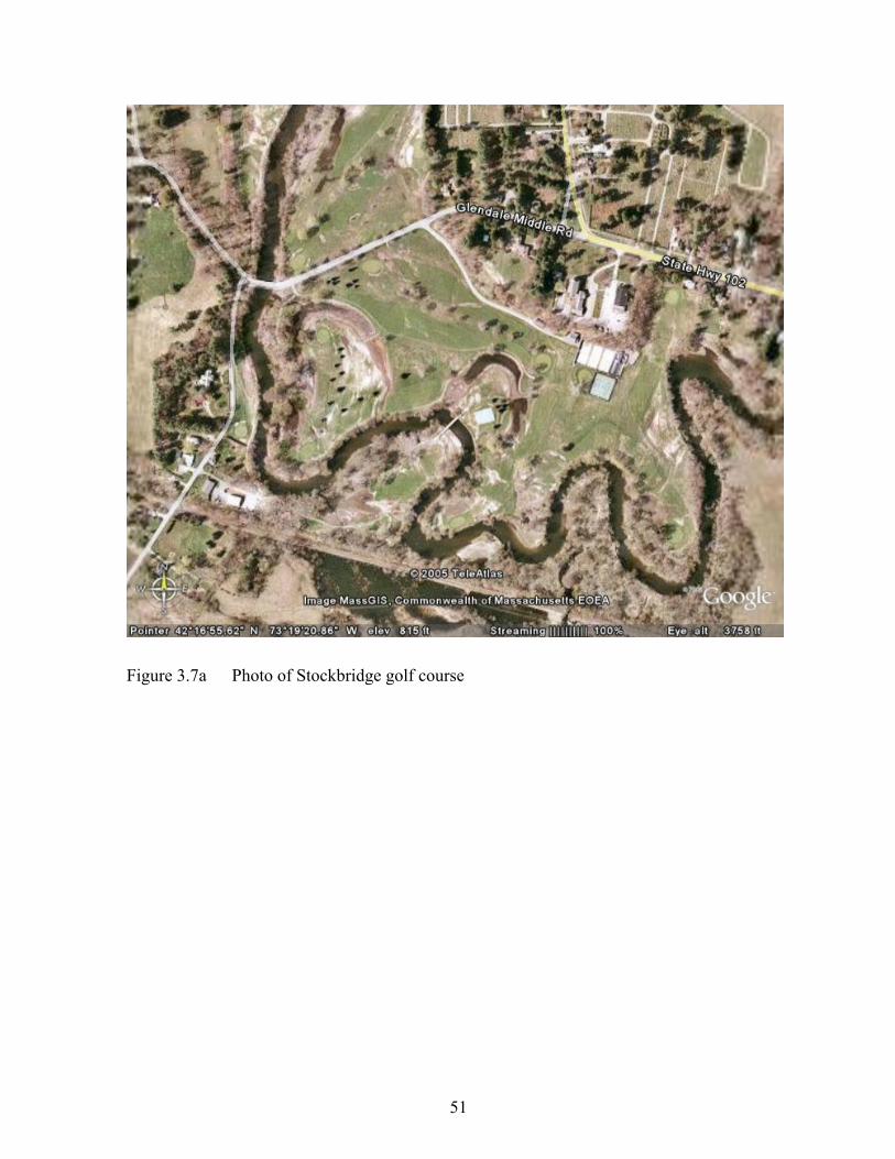
Figure 3.7a Photo of Stockbridge golf course

51

Housatonic River Downstream Model

Bottom Elev245 4018.00 255

Figure 3.7b Grid in the area of the Stockbridge golf course. North is up in this figure.

52

Figure 3.8 Initial Longitudinal Distributions of Grain Sizes for the River Bed Sediment

53

Figure 3.9 Initial Longitudinal Distributions of Bulk Densities for the River Bed Sediment

54

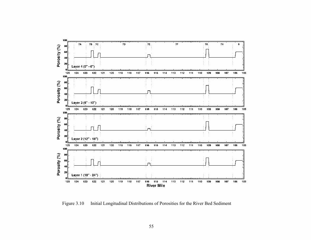
Figure 3.10 Initial Longitudinal Distributions of Porosities for the River Bed Sediment

55

Figure 3.11 Initial Longitudinal Distributions of Sediment Bed PCB Concentrations for the River Bed Sediment

56

Figure 3.12 Initial Longitudinal Distributions of Fractions of Organic Carbon for the River Bed Sediment

57

58

OC Normalized PCBs, Individual Samples and 1 Mile Bins

1

10

100

1000

104109114119124

River Mile

PCB

s, u

g/g

OC

OC Normalized PCBs, Individual Samples and 1 Mile Bins

0

100

200

300

400

500

600

700

800

900

1000

104109114 119124

River Mile

PCB

s, u

g/g

OC

Figure 3.13 Initial OC-Normalized PCB Concentrations (Segregated into 1-Mile Bins) versus River Mile (after WESTON, 2006)

59

4 MODEL EVALUATION 4.1 Model Application

The EFDC model was run to simulate sediment and tPCB transport in Reaches 7 and 8 over an 11-year period, from January 1, 1994 – December 31, 2004. This period was selected because it includes the vast majority of the data record available for Reaches 7 and 8. For the simulation, the EFDC model was spun-up using the boundary conditions for the one year period prior to January 1, 1994. The simulated sediment bed conditions at the end of this one year spin-up were used as the initial conditions for the simulation. The initial PCB concentrations at the beginning of the 11-year simulation were set equal to those at the beginning of the one-year spin-up run since these initial concentrations were determined from data.

4.2 Model-Data Comparisons for Water Column TSS and PCBs

The only data set for water column PCB and TSS concentrations used to develop model-data comparisons was collected at Division Street (the USGS Great Barrington gaging station), located approximately 1 mile downstream of Rising Pond Dam. Simulated TSS and tPCB concentrations at the outlet of Rising Pond (shown as black lines) are compared with the data (shown as red squares) in Figures 4.1a through 4.1f in which the state variable is plotted on a log scale. To make it easier to visualize the differences between model results and data, model results corresponding to the time of data collection are indicated by blue open circles on days when TSS or tPCB data were collected. Few data were collected in 1994-1995 (Figure 4.1a). However, in subsequent years, the sampling frequency increased to bimonthly to monthly in most periods, and more frequently in some periods. In particular, there was a period from April to May 1997 when relatively high frequency TSS sampling was conducted.

TSS concentrations measured at the outlet of Rising Pond were typically in the range of 1.5 to 15 mg/L. The low end of the range of simulated TSS concentrations decreases to approximately 2.0 mg/L during low-flow conditions, consistent with the data. Simulated TSS concentrations vary in response to changes in the hydrograph (upper panel), reaching values greater than 100 mg/L several times per year. Data are typically not available at the time of these simulated peak TSS concentrations. However, during March - May 1997, two high flow events with peak flows greater than 1,000 cfs occurred. TSS measurements through this period ranged from approximately 3 to 30 mg/L and showed considerable scatter. The TSS data also exhibited a relationship (within the scatter) with flow corresponding to the peak flows of the two events. Simulated TSS values during this period are well within the range of the measurements, and also capture some of the relationship exhibited by the measurements. For example, the simulated and measured peak TSS values are similar. Throughout the remainder of the simulation period, the model results are in general agreement with the data, but sometimes underestimate the measurements. The simulated TSS values are also typically less variable than the measurements. These differences may be attributable, at least in part, to differences between the HSPF simulated nonpoint runoff and the flows and solids loadings from the seven modeled tributaries that are used as input to the EFDC model compared with the actual flows and loadings. That is, it needs to be recognized that at the relatively fine temporal and spatial resolution of the EFDC model application, even small differences in the timing and magnitude of HSPF simulated inputs could

60

cause comparatively large differences between simulation results and measurements. For example, Figure 4.2 shows the model-data comparisons for the April to June 1997 period. The upper panel shows the comparison between the simulated flow (solid blue line) at Rising Pond Dam and the measured flow at Division Street. As observed, the simulated flows are higher than the measured flows for most of this three month period. While the TSS data are generally higher than the simulated values, the vast majority of the differences are less than 5 mg/L, and thus within the uncertainty associated with the measured values since the latter are based on samples collected at one point in the cross-section at Division Street and the simulated values are the cross-sectionally averaged values at the outflow from Rising Pond. Figure 4.3 shows the model-data comparison for July – September 2004. Notwithstanding the extremely limited number of measurements, the level of agreement seen in this figure between measured and simulated flows and between the three measured values of TSS and tPCB and the simulated values is representative of the model-data agreement achieved in the last six years of the 11-year simulation.

Comparisons between simulated and measured tPCBs show similar behavior to that described for TSS. Measured tPCB values vary narrowly from ~0.01 to ~0.05 µg/L and do not show pronounced temporal (e.g., seasonal) trends over time. Model results are consistently within this range. However, the data are definitely impacted by changes in detection limits. For example, model results overestimate measured tPCB concentrations when the detection limits are lower, and at other times when detection limits are higher, the model results underestimate tPCB concentrations. Overall, model results overestimate tPCB concentrations. However, as described previously, this is likely a consequence of the differences between the actual watershed inputs and those generated by HSPF.

4.3 Model Results for Sediment PCB Concentrations

Daily and spatially averaged (over each of the nine FCM reaches) organic carbon (OC) normalized sediment tPCB concentrations over the 11-year simulation are shown in Figure 4.4. In the majority of the modeling domain, sediment PCB exposure concentrations change by relatively small amounts (less than +10%) over the 11-year simulation. Subreaches where simulated changes were outside this range are limited to Reaches 7B (-17% change) and 7F (71% change). The large increase in Reach 7F represents an increase in the tPCB concentration from less than 40 to almost 70 mg/kg OC over the simulation period. This large relative percent increase is attributed, at least in part, to uncertainty in the initial conditions for sediment tPCB concentrations. Initial conditions in each of the flowing reaches (between impoundments) are characterized by more uncertainty than impounded reaches because of varying sample density in the different reaches. Sampling programs were targeted toward reaches that were more depositional in character, e.g., impoundments. These included reaches 7B, 7E, 7G, and 8. Because of the more limited number of samples collected in the flowing reaches, data from all of these reaches were aggregated to develop an average initial tPCB concentration that was assigned to each of the flowing reaches. Reach 7F has the smallest bed slope of the flowing reaches, making it more conducive to deposition than the other similar reaches. The increase in sediment tPCB concentrations simulated in Reach 7F reflects net deposition in that reach. This is further discussed in Section 4.5.

61

4.4 Evaluation of Model Performance

Figures 4.5 and 4.6 show plots (hereafter called cross-plots) of simulated versus measured TSS and tPCB concentrations, respectively. The differences between measured and simulated concentrations shown in these figures are attributed to, in part, phasing differences between the simulated results at Rising Pond Dam and the data collected from Division Street. Phasing and volumetric differences between actual flows (runoff and tributaries in Reach 7) and HSPF-simulated flows from these sources contribute to the phasing difference between tPCB and TSS water column data and EFDC simulated concentrations. This factor accounts for some differences where the simulated tPCB concentrations are, for example, lower than the measured values due to HSPF-simulated flows that are higher than actual flows, resulting in lower simulated tPCB concentrations due to dilution.

As shown in Figure 4.5, a considerable number of model-data comparisons follow the one-to-one line, with simulated values within a factor of 2 or 3 of the data. There is also a sizable group of data that vary between 2 and 15 mg/L, with corresponding simulated TSS concentrations falling within a narrow range of 2 to 4 mg/L (these appear as a dark band in Figure 4.5). The regression of simulated versus measured TSS is strongly influenced by this little group of model-data pairs because of the number of points falling within this group. Data within this group could reflect variation from the data do to a variety do causes, but some of the comparisons are likely influenced by the fact that the simulated hydrograph did not increase as quickly as the actual flows. At the upper end of the range of simulated TSS concentrations, the simulated concentrations exceed the measured concentrations, corresponding to transient flow events when phase differences between simulated and measured hydrographs would be more pronounced.

The cross-plot of simulated and measured tPCB concentrations (Figure 4.6) include only data for which sampling times were reported. The phasing issue discussed for TSS is further exacerbated when the concentration data record does not include the time of sampling needed to properly associate the data with the model output; therefore, these data were not included in the cross-plot. For the majority of the detected concentrations, the simulated concentrations were within a factor of two of the measured values, including elevated concentrations near 0.06 and 0.1µg/L that are very close to the one-to-one line. Approximately 70% of the data were non-detects (plotted at the detection limit) and the simulated concentrations at the sampling times were typically near the detection limit. The one exception to this was a group of data collected in 1998 that had a relatively high detection limit of 0.125 µg/L. Given the range of the detected concentrations, it is unlikely that the actual tPCB concentrations were near this detection limit.

There are six model-data comparisons (with detected concentrations) for which the simulated concentrations are not within a factor of two of the data. These points fall below the one-to-one line and have a substantial effect on the regression of simulated versus measured tPCB concentrations, that yields a slope of 0.27 and r2 = 0.17 if these points are excluded. The highest tPCB concentration (0.26 µg/L) was measured during the October 2003 high-flow event. The tPCB concentration simulated at the exact time the sampling was conducted was 0.06µg/L; however, simulated concentrations increased to approximately 0.2µg/L during that storm, consistent with the magnitude of the measured concentration. This model-data comparison highlights the significant effect that differences in the timing of actual and simulated hydrographs have on the comparison of simulated and measured water column tPCB concentrations.

62

Probability distributions of simulated and measured TSS and tPCB concentrations are presented in Figures 4.7 and 4.8, respectively. In general, the simulated concentrations have somewhat less variability than the measured concentrations, with the exception being the upper 5% of the TSS data. TSS concentrations above 20 mg/L reflect increased flow conditions when phasing issues are more pronounced. The elevated tPCB detection limits for samples collected in 1998 complicate the comparison of the simulated and measured tPCB distributions shown in Figure 4.8 because the actual concentrations could be substantially lower. This would shift the detected concentrations above 0.04 µg/L to the right on the plot, i.e., they would be less frequent occurrences.

A statistical summary of the performance of the EFDC model for TSS and tPCB concentrations is presented in Table 4.1. The Modeling Study QAPP (WESTON, 2000) presents model performance measures for these and other model outputs. As shown in Table 4.1, the relative bias at Rising Pond outlet is well within the model performance measure of ± 30% for the TSS (-11.93%) and just outside the measure for PCB concentration (-31.97%). For median relative error, the model performance measure is also ± 30%, and the EFDC model is within the performance measure for both TSS (-27.12%) and PCB concentration (-3.32%).

4.5 Process-Based Flux Summaries

Process-based annual average mass fluxes for solids and PCBs calculated by the EFDC model for Reaches 7 and 8 are presented in Figures 4.9 and 4.10 and summarized in Tables 4.2 and 4.3. The various mass fluxes in these summaries were not expected to balance exactly because of rounding/truncation in the summation of the mass fluxes across each cell face at each time step of the simulation. The residuals of the balance of the process-based annual average mass flux terms represent a small fraction (0.1 to 6%) of the total annual mass flux into each reach.

Solids mass fluxes are dominated by the water column advective fluxes, and increase substantially in Reach 7D due to inputs from tributaries and direct runoff, both of which are simulated by HSPF. Spatial patterns of erosion reflect the armored bed conditions in the steep reaches (7A, 7C, upper half of 7D, and 7H). Milder slopes in the lower half of Reach 7D and in Reach 7F result in relatively high deposition and high erosion rates that produce a relatively small net erosion flux in Reach 7D and a small net deposition flux in Reach 7F. Although these two reaches have the smallest bottom slopes (i.e., gradients), relatively high erosion rates occur during the rising limbs of runoff hydrographs, when previously deposited sediment is rapidly eroded due to high bed shear stresses. Deposition on the floodplain is greatest in Reaches 7D and 7F, where the floodplain is considerably wider than in the other reaches domain. Bedload mass fluxes of solids vary through the domain in response to the armoring conditions in the steeper reaches and the physical barriers of the dams.

Water column advective PCB mass fluxes do not vary substantially through Reaches 7 and 8, decreasing from 29 kg/yr at the upstream boundary to 25.5 kg/yr at the downstream boundary. PCB transport associated with bedload is a very small part of the overall PCB transport balance, with annual average fluxes less than 0.005 kg/yr. PCB transport associated with sediment erosion is higher in the impoundments of Columbia Mill Dam (Reach 7B), Willow Mill Dam (Reach 7E), Glendale Dam (Reach 7G) and Rising Pond Dam (Reach 8) than in the

63

steep-sloped flowing sections of the river. These higher PCB mass fluxes result from higher tPCB concentrations in the impoundment sediment that are in turn related to higher fractions of fine sediment with relatively higher organic carbon content. In Reaches 7D and 7F, PCB mass fluxes associated with erosion are comparable to those in the impoundment reaches because of the relatively higher rates of erosion during the rising limbs of runoff hydrographs.

As expected, depositional mass fluxes of PCBs are related to bed slope, with the highest rates in impoundments and in the lower gradient reaches of 7D and 7F. Generally, deposition rates on the floodplain are small, with the highest rates on the wider floodplains of the lower half of Reach 7D and Reach 7F. Overall, volatilization losses represent approximately 11% of the PCB inputs entering at the upstream boundary (Woods Pond Dam). Volatilization losses from the river account for almost 90% of the total volatilization loss. The remainder is lost from water transported across the floodplain.

The process-based annual average mass flux summaries highlight the processes controlling solids and PCB transport through Reaches 7 and 8. The interactive effect of the different bed slopes and solids composition characteristics of the flowing sections and impoundments is seen in the relative magnitude of the various mass fluxes in these different reaches. For example, although Reaches 7D and 7F have relatively high solids erosion rates, the lower PCB concentrations in these long flowing sections result in PCB mass fluxes that are less than the PCB mass fluxes in the relatively short impoundments, where higher fractions of fine-grained sediment are found. These summaries provide an additional tool for understanding the major processes controlling PCB fate in Reaches 7 and 8.

64

Table 4.1

Statistical Evaluation of EFDC Model Performance, January 1994 – December 2004

Statistical Summary of EFDC Model Performance

Station No. of Data

(n) Average of

Data Model Bias Arithmetic

Model Bias

Geometric Relative Bias (%)

Mean Absolute

Error

Median Relative

Error (%)

Regression of Simulated vs. Measured Values

Slope Y-

Intercept

Coefficient of Determination

(r2)

TSS (mg/L)

Rising Pond Outlet 177 6.82 -0.81 0.77 -11.93 4.88 -27.12 0.31 0.90 0.11

PCB (µg/L)

Rising Pond Outlet 28 0.055 -0.02 0.77 -31.97 0.02 -3.32 0.27 -2.52 0.17

65

Table 4.2

Process-Based Annual Average Mass Flux Summary Tabulation for Solids

Channel/Floodplain Process Solids Flux (MT/yr)

7A 7B 7C 7D 7E 7F 7G 7H 8

Channel Water Column Sources Advection 2352.4 2349.0 2520.0 2546.0 4235.0 4315.0 4677.0 4826.0 4769.0 Bed load 0.0 6.1 0.0 13.1 0.0 0.0 223.1 0.0 27.8 Import from Floodplain 141.8 33.0 272.0 HSPF Tributary and Surface Runoff 188.9 10.9 0.8 1928.3 1.8 563.9 1.0 2.6 1.9 Erosion 68.3 263.0 88.5 2793.4 512.0 3467.2 273.4 410.7 1215.8 Sum 2609.7 2770.8 2642.3 7280.8 4748.8 8618.1 5174.5 5239.3 6014.4

Channel Water Column Sinks Downstream Advection 2349.0 2520.0 2546.0 4235.0 4315.0 4677.0 4826.0 4769.0 4663.8 Bed load 6.1 0.0 13.1 0.0 0.0 223.1 0.0 27.8 0.0 Export to Floodplain 189.0 279.4 21.5 156.6 44.5 184.1 Deposition 65.6 250.8 83.2 2766.4 412.3 3718.0 191.9 398.1 1166.6 Sum 2609.7 2770.8 2642.3 7280.8 4748.8 8618.1 5174.5 5239.3 6014.4

Floodplain Water Column Sources Import from Channel 189.0

279.4

21.5

156.6

44.5 184.1 Overland Flow 189.9 0.0 12.8 -4.4 0.0 0.2 0.0 0.0 Erosion 10.2 12.0 3.4 579.9 0.0 516.6 33.2 2.3 22.2 Sum 199.2 201.8 3.4 872.1 17.1 516.6 189.9 46.7 206.3

Floodplain Water Column Sinks Export to Channel 141.8 33.0 272.0 Overland Flow 189.9 0.0 12.8 -4.4 0.0 0.2 0.0 0.0 0.0 Deposition 9.1 14.4 9.1 714.5 0.0 529.9 76.8 38.4 154.5 Sum 199.0 156.2 54.8 710.1 0.0 802.1 76.8 38.4 154.5

Reach Residual 0.2 45.6 -51.4 162.1 17.1 -285.4 113.2 8.3 51.8

66

Table 4.3

Process-Based Annual Average Mass Flux Summary Tabulation for PCBs

Channel / Floodplain Process PCB Flux (kg/yr) 7A 7B 7C 7D 7E 7F 7G 7H 8

Channel Water Column Sources Advection 29.04 26.10 28.80 28.40 25.80 25.70 23.50 24.30 23.80 Bed load 0.00 0.00 0.00 0.00 0.00 0.00 0.00 0.00 0.00 Import from Floodplain 2.68 0.06 0.18 0.02 Diffusion 0.00 0.09 0.02 0.12 0.02 0.12 0.02 0.01 0.20 Erosion 0.00 0.24 0.02 0.21 0.28 0.44 0.70 0.01 1.78 Sum 29.04 29.11 28.83 28.73 26.10 26.32 24.39 24.34 25.78

Channel Water Column Sinks Downstream Advection 26.10 28.80 28.40 25.80 25.70 23.50 24.30 23.80 25.51 Bed load 0.00 0.00 0.00 0.00 0.00 0.00 0.00 0.00 0.00 Export to Floodplain 2.62 0.23 0.24 0.06 Volatilization 0.31 0.15 0.15 0.86 0.06 0.62 0.03 0.38 0.29 Deposition 0.01 0.16 0.05 1.82 0.28 2.20 0.06 0.16 0.53 Sum 29.04 29.11 28.83 28.73 26.10 26.32 24.39 24.34 26.33

Floodplain Water Column Sources Import from Channel 2.62 0.23 0.24 0.06 0.00 Overland Flow 2.59 0.00 0.20 0.01 0.00 0.00 0.00 0.03 Diffusion 0.00 0.01 0.00 0.14 0.01 0.10 0.00 0.00 0.00 Erosion 0.01 0.03 0.00 0.38 0.01 0.47 0.04 0.00 0.00 Sum 2.63 2.62 0.23 0.95 0.07 0.57 0.04 0.00 0.04

Floodplain Water Column Sinks Export to Channel 2.68 0.06 0.18 0.02 Overland Flow 2.59 0.00 0.20 0.01 0.00 0.00 0.00 0.03 Volatilization 0.03 0.01 0.00 0.19 0.01 0.18 0.01 0.00 0.01 Deposition 0.00 0.01 0.03 0.89 0.00 0.54 0.03 0.02 0.01 Sum 2.62 2.70 0.22 1.09 0.01 0.78 0.22 0.07 0.02

Reach Residual 0.01 -0.08 0.00 -0.14 0.07 -0.20 -0.18 -0.07 -0.53

67

Figure 4.1a Comparison of Simulated (Solid Line) and Measured (Red Symbols) TSS and tPCB Concentrations in the Water Column for 1994-1995. DL = detection limit

68

Figure 4.1b Comparison of Simulated (Solid Line) and Measured (Red Symbols) TSS and tPCB Concentrations in the Water Column for 1996-1997. DL = detection limit

69

Figure 4.1c Comparison of Simulated (Solid Line) and Measured (Red Symbols) TSS and tPCB Concentrations in the Water Column for 1998-1999. DL = detection limit

70

Figure 4.1d Comparison of Simulated (Solid Line) and Measured (Red Symbols) TSS and tPCB Concentrations in the Water Column for 2000-2001. DL = detection limit

71

Figure 4.1e Comparison of Simulated (Solid Line) and Measured (Red Symbols) TSS and tPCB Concentrations in the Water Column for 2002-2003. DL = detection limit

72

Figure 4.1f Comparison of Simulated (Solid Line) and Measured (Red Symbols) TSS and tPCB Concentrations in the Water Column for 2004. DL = detection limit

73

Figure 4.2 Comparison of Simulated (Solid Line) and Measured (Red Symbols) TSS and tPCB Concentrations in the Water Column for April – June 1997. DL = detection limit

74

Figure 4.3 Comparison of Simulated (Solid Line) and Measured (Red Symbols) TSS and tPCB Concentrations in the Water Column for July – September 2004. DL = detection limit

75

450 tP

CB

in S

urfa

ce S

edim

ent (

mg/

kg O

C) 400

350

300

250

200

150

100

50

0 Jan-94 Jan-95 Jan-96 Jan-97 Jan-98 Jan-99 Jan-00 Jan-01 Jan-02 Jan-03 Jan-04

Reach 7A Reach 7B Reach 7C Reach 7D Reach 7E

Reach 7F Reach 7G Reach 7H Reach 8

Note: Colored circle symbols indicate sediment initial conditions used at the beginning of EFDC spin-up.

Figure 4.4 Temporal Trend of tPCB Concentrations in Surface Sediments for Foodchain Reaches

76

Figure 4.5 Cross-Plot of Simulated and Measured TSS Concentrations

77

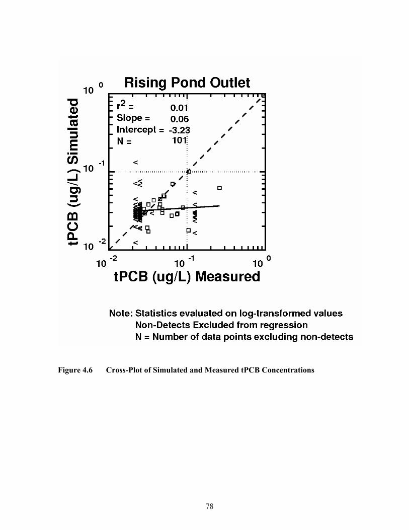
Figure 4.6 Cross-Plot of Simulated and Measured tPCB Concentrations

78

Figure 4.7 Probability Distributions of Simulated and Measured TSS Concentrations

79

Figure 4.8 Probability Distributions of Simulated and Measured tPCB Concentrations

80

Figure 4.9 Process-Based Annual Average Mass Flux Summary for Solids

81

Figure 4.10 Process-Based Annual Average Mass Flux Summary for PCBs

82

5 CONCLUSION

As stated in Section 1, the purpose of this modeling effort was to evaluate the ability of EFDC, the state-of-the-art contaminated sediment modeling system, to simulate the transport and fate of a contaminant over a time period of at least 10 years. Evaluation of the results of an 11­year simulation using the minimally calibrated EFDC Model indicate that this model is capable of simulating the transport and resultant concentrations of TSS and PCBs in Reaches 7 and 8 of the Housatonic River within the specified model performance measures. Specifically, a statistical summary of the performance of the EFDC model for TSS and PCB concentrations found that the relative bias at Rising Pond outlet is well within the model performance measure of ± 30% for TSS (-11.93%) and just outside the measure for PCB concentrations (-31.97%). For median relative error, the model performance measure is also ± 30%, and the EFDC model is within the performance measure for both TSS (-27.12%) and PCB (-3.32%) concentrations. Considering the fact that the model was only minimally calibrated, and that the system modeled had widely varying hydraulic and morphologic regimes, the EFDC model’s performance, as quantified by the relative bias and the median relative error, is considered good. This demonstrates that EFDC is a robust modeling system that can be successfully implemented at other contaminated sediment sites.

83

REFERENCES

Arega, F. W., and E. J. Hayter (2006). “Skill Assessment of EFDC - a 3D Hydrodynamic and Transport Model - to Simulate Highly Stratified Estuarine Flows”, submitted to Journal of Estuarine, Coastal and Shelf Science in April 2006.

Ariathurai, R. (1974). “A Finite Element Model for Sediment Transport in Estuaries”, Ph.D. Dissertation, University of California, Davis, California.

Ariathurai, R., and K. Arulanandan (1978). “Erosion Rates of Cohesive Soils”, Journal of the Hydraulics Division, ASCE, 104(HY2), 279-283.

Aris, R. (1956). “On the Dispersion of a Solute in a Fluid Flowing Through a Tube”, Proceedings Royal Society of London, Series A, 235, 67-77.

Bain, A. J. (1981). “Erosion of Cohesive Muds”, M.S. Thesis, University of Manchester, United Kingdom, 1981.

Barnes, R. S. K., and J. Green, Editors. (1971). The Estuarine Environment, Applied Science Publishers, London.

BBL (Blasland, Bouck & Lee, Inc.) (1994). MCP Interim Phase II Report and Current Assessment Summary for East Street Area 2/U.S. EPA Area 4. Volumes I, II, III, IV, V, VI, VII, IX, X, and XII.

BBL (Blasland, Bouck & Lee, Inc) and QEA (Quantitative Environmental Analysis, LLC). (2003). Housatonic River – Rest of River RCRA Facility Investigation Report. Prepared for General Electric Company, Pittsfield, MA.

Been, K., and G. C. Sills. (1981). “Self-weight Consolidation of Soft Soils: An Experimental and Theoretical Study,” Geotechnique, 31(4), 519-535.

Bellessort, B. (1973). “Movement of Suspended Sediments in Estuaries-Flocculation and Rate of Removal of Muddy Sediments,” Tracer Techniques in Sediment Transport, International Atomic Energy Agency, Technical Report Series No. 145, 31-40.

Burkhard, L.P. (2000). “Estimating dissolved organic carbon partition coefficients for nonionic organic chemicals”, Environmental Science and Technology 34(22):4663-4668.

Burt, T. N., and W. R. Parker. (1984). “Settlement and Density in Beds of Natural Mud During Successive Sedimentation”, Report IT 262, Hydraulics Research, Wallingford, United Kingdom.

84

Christensen, B. A. (1965). “Discussion of ‘Erosion and Deposition of Cohesive Soils’,” by Partheniades, E., Journal of the Hydraulics Division, ASCE, 91(HY5), 301.

Christensen, R. W., and B. M. Das. (1973). “Hydraulic Erosion of Remolded Cohesive Soils,”Special Report 135, Highway Research Board, Washington, D.C., 8-19.

Chang, F. M., D. B. Simons, and E. V. Richardson. (1965). “Total Bed-Material Discharge in Alluvial Channels,” U.S. Geological Survey Water-Supply Paper 1498-I. Engelund, F. and E. Hansen (1967). A monograph on sediment transport in alluvial streams, Teknisk Forlag, Copenhagen, Denmark. 62 pp.

Chapra, S. C. (1997). Surface Water-Quality Modeling, McGraw-Hill Companies, Inc.

Di Toro, D.M. (1984). “Probability model of stream quality due to runoff”, Journal of Environmental Engineering. ASCE 110(3):607-628.

Di Toro, D.M. (1985). “A particle interaction model of reversible organic chemical sorption”, Chemosphere 14(10):1503-1538.

Di Toro, D.M., C.S. Zarba, D.J. Hansen, W.J. Berry, R.C. Swartz, C.E. Cowan, S.P. Pavlou, H.E. Allen, N.A. Thomas, and P.R. Paquin. (1991). “Technical basis for establishing sediment quality criteria for nonionic organic chemicals by using equilibrium partitioning”, Environmental Toxicology and Chemistry 10:1541-1583.

Di Toro, D.M. (2000). Sediment Flux Modeling. John Wiley & Sons, Inc, New York, NY.

Dixit, J. G. (1982). “Resuspension Potential of Deposited Kaolinite Beds,” M.S. Thesis, University of Florida, Gainesville, Florida.

Dyer, K. R. (1986). Coastal and Estuarine Sediment Dynamics, John Wiley and Sons, London.

Dyer, K. R. (1989). “Sediment processes in estuaries: future research requirements,” Journal of Geophysical Research, 94(C10), 14327-14339.

Edzwald, J. K., J. B. Upchurch, and C. R. O'Melia. (1974). “Coagulation in Estuaries,” Environmental Science and Technology, 8(1), 58-63.

Einstein, H. A. (1950). “The Bed-Load Function for Sediment Transportation in Open Channel Flows,” U.S. Department of Agriculture, Soil Conservation Service, Technical Bulletin no. 1026.

Einstein, H. A., and N. L. Barbarossa. (1952). “River Channel Roughness,” Transactions of the ASCE, 117, 1121-1132.

85

Einstein, H. A., and R. B. Krone. (1962). “Experiments to Determine Modes of Cohesive Sediment Transport in Salt Water,” Journal of Geophysical Research, 67(4), 1451-1464.

Fischer, H. B. (1966). “Longitudinal Dispersion in Laboratory and Natural Streams,” Ph.D. Dissertation, California Institute of Technology, Pasadena, California.

Fischer, H. B. (1972). “Mass Transport Mechanisms in Partially Stratified Estuaries,” Journal of Fluid Mechanics, 53(4), 671-687.

Fischer, H. B., J. Imberger, E. J. List, R. C. Y. Koh, and N. H. Brooks. (1979). Mixing in Inland and Coastal Waters, Academic Press, New York.

Galperin, B., L. H. Kantha, S. Hassid, and A. Rosati (1988). “A Quasi Equilibrium Turbulent Energy Model for Geophysical Flows”, Journal of Atmospheric Science, 45, pp. 55-62.

Garcia, M., and G. Parker (1991). “Entrainment of bed sediment into suspension”, J. Hyd. Engrg., 117, 414-435.

Gessler, J. (1965). “The Beginning of Bedload Movement of Mixtures Investigated as Natural Armoring in Channels,” W. M. Keck Laboratory of Hydraulics and Water Resources, California Institute of Technology, Pasadena.

Gessler, J. (1970). “Self-stabilizing Tendencies of Alluvial Channels,” Journal of the Waterways and Harbors Division, ASCE, 96(WW2), 235-249.

Grim, R. E. (1968). Clay Mineralogy, McGraw-Hill, New York.

Grimshaw, R. W. (1971). The Chemistry and Physics of Clays, Wiley-Interscience, New York.

Hamrick, J. M. (1992). “A Three-Dimensional Environmental Fluid Dynamics Computer Code: Theoretical and Computational Aspects”, Special Report No. 317 in Applied Marine Science and Ocean Engineering, Virginia institute of Marine Science, Gloucester Point, VA., pp. 1-64.

Hamrick, J. M and W. B. Mills (2000). “Analysis of Water Temperatures in Conowingo Pond as Influenced by the Peach Bottom Atomic Power Plant Thermal Discharge”, Environmental Science and Policy, 3(1), pp. 197-209.

Hanzawa, H., and T. Kishida. (1981). “Fundamental Considerations of Undrained Strength Characteristics of Alluvial Marine Clays,” Soils and Foundation, Japanese Society of Soil Mechanics and Foundation Engineering, 21(1), 39-50.

Harza. (2001). Woods Pond Dam: Structural Integrity Assessment. Prepared for General Electric Company, Pittsfield, MA.

86

Hawker, D. W., and D. W. Connell. (1988). “Octanol-water partition coefficients of polychlorinated biphenyl congeners”, Environmental Science and Technology, 22:382-387.

Hayter, E. J. (1983). “Prediction of the Movement of Cohesive Sediments in Estuarial Waters,” Ph.D. Dissertation, University of Florida, Gainesville, Florida.

Hayter, E. J., Bergs, M., Gu, R., McCutcheon, S., Smith, S. J., and Whiteley, H. J. (1999). “HSCTM-2D, A Finite Element Model for Depth-Averaged Hydrodynamics, Sediment and Contaminant Transport”, Technical Report, EPA Ecosystems Research Division, Athens, Georgia.

Hayter, E. J., V. Paramygin, and C. V. John. (2003). A3D Modeling of Cohesive Sediment Transport in a Partially Stratified Microtidal Estuary to Assess Effectiveness of Sediment Traps”, 7th International Conference on Nearshore and Estuarine Cohesive Sediment Transport Processes, Virginia Institute of Marine Science, Gloucester Point, VA, October 2003.

Holley, E. R. (1969). “Unified View of Diffusion and Dispersion,” Journal of the Hydraulics Division, ASCE, 95(HY2).

Holley, E. R., D. R. F. Harleman, and H. B. Fischer. (1970). “Dispersion in Homogeneous Estuary Flow,” Journal of the Hydraulics Division, ASCE, 96(HY8), 1691-1709.

Hunt, J. R. (1980). “Prediction of Ocean Particle Size Distribution from Coagulation and Sedimentation Mechanisms,” Advances in Chemistry Series No. 189 - Particles in Water, M. D. Kavanaugh and J. O. Keckie, Editors, American Chemical Society, Washington, D.C., 243-257.

Imhoff, J. C., A. Stoddard, and E. M. Buchak (2003). “Evaluation of Contaminated Sediment Fate and Transport Models”, Final Report, U.S. EPA, National Exposure Research Laboratory, Athens, GA.

Imhoff, J.C., J. Clough, R.A. Park, and A. Stoddard (2004). “Evaluation of Chemical Bioaccumulation Models for Aquatic Ecosystems”, Final Report, U.S. EPA, National Exposure Research Laboratory, Athens, GA, 122 pp.

Jepsen, R., J. Roberts, and W. Lick. (1997). “Effects of Bulk Density on Sediment Erosion Rates,” Water, Air, and Soil Pollution, 99, 21-31.

Ji, Z.-G., M. R. Morton, and J. M. Hamrick (2000). “Modeling Hydrodynamic and Sediment Processes in Morro Bay”, Estuarine and Coastal Modeling: Proc., 6th Int. Conf., M. L. Spaulding and H. L. Butler, eds., ASCE, New York, pp. 1035-1054.

Ji, Z.-G., M. R. Morton, and J. M. Hamrick (2001). “Wetting and Drying Simulation of Estuarine Processes”, Estuarine, Coastal Shelf Sci. 53( 5), pp. 683-700

Jin, K. R., Z.-G. Ji, and J. M. Hamrick (2002). “Modeling Winter Circulation in Lake

87

Okeechobee, Florida,” Journal of Waterways, Port, Coastal, Ocean Eng., 128(3), pp. 114-125.

Jin, K.-R., J. M. Hamrick, and T. Tisdale (2000). “Application of a Three Dimensional Hydrodynamic Model for Lake Okeechobee,” Journal of Hydraulic Engineering, 126(10), pp. 758-771.

Jobson, H. E., and W. W. Sayre. (1970). “Vertical Transfer in Open Channel Flow,” Journal of the Hydraulics Division, ASCE, 96(HY3), 703-724.

Kandiah, A. (1974). “Fundamental Aspects of Surface Erosion of Cohesive Soils,” Ph.D. Dissertation, University of California, Davis, California.

Karcz, I., and G. Shanmugam. (1974). “Decrease in Scour Rate of Fresh Deposited Muds,” Journal of the Hydraulics Division, ASCE, 100(HY11), 1735-1738.

Karickhoff, S. W., D. S. Brown, and T. A. Scott. (1979). “Sorption of hydrophobic pollutants on natural sediments”, Water Research 13:241-248.

Karickhoff, S. W. (1981). “Semi-empirical estimation of sorption of hydrophobic pollutants on natural sediment and soils”, Chemosphere 10(8):833-846.

Karickhoff, S. W. (1984). “Organic pollutant sorption in aquatic systems”, ASCE, J. Hydraulic Engineering 110(6):707-735.

Kelley, W. E., and R. C. Gularte. (1981). “Erosion Resistance of Cohesive Soils,” Journal of the Hydraulics Division, ASCE, 107(HY10).

Kim, S., D. L. Wright, J. Maa and J. Shen (1997). “Morphodynamic Responses to Extra Tropical Meteorological Forcing on the Inner Shelf of the Middle Atlantic Bight: Wind Wave, Currents and Suspended Sediment Transport”, Proc. of Estuarine and Coastal Modeling, pp. 456-66.

Kirby, R., and W. R. Parker. (1977). “The Physical Characteristics and Environmental Significance of Fine Sediment Suspensions in Estuaries,” Estuaries, Geophysics and the Environment, National Academy of Sciences, Washington, D.C., 110-120.

Kranck, K. (1980). “Sedimentation Processes in the Sea,” The Handbook of Environmental Chemistry, 2(A), O. Hutzinger, Editor, Springer-Verlag, Berlin, 61-75. Krone, R. B. (1962). “Flume Studies of the Transport of Sediment in Estuarial Shoaling Processes,” Final Report, Hydraulic Engineering Laboratory and Sanitary Engineering Research Laboratory, University of California, Berkeley, California.

Krone, R. B. (1963). “Study of Rheological Properties of Estuarial Sediments,” Technical Bulletin No. 7, Committee of Tidal Hydraulics, U.S. Army Corps of Engineers, Vicksburg, Mississippi.

88

Krone, R. B. (1972). “Field Study of Flocculation as a Factor in Estuarial Shoaling Processes,” Technical Report No. 19, Committee on Tidal Hydraulics, U.S. Army Corps of Engineers, Vicksburg, Mississippi.

Lambermont, J., and T. Lebon. (1978). “Erosion of Cohesive Soils,” Journal of Hydraulic Research, 16(1), 27-44.

Lee, P. T. (1974). “Deposition and Scour of Clay Particles Due to Currents,” M.S. Thesis, Asian Institute of Technology, Bangkok, Thailand.

Lick, W., J. Lick, and C. K. Ziegler (1994). “The resuspension and transport of fine-grained sediments in Lake Erie”, Journal of Great Lakes Research 20(4):599-612.

Mathew, R. M., E. J. Garland, and P. R. Paquin. (2002). “Partitioning of PCBs and importance to fate and effects”, Presented at the 2002 North American SETAC Conference, Salt Lake City, UT, November 2002.

McNeil, J., C. Taylor, and W. Lick. (1996). “Measurements of the Erosion of Undisturbed Bottom Sediments with Depth,” Journal of Hydraulic Engineering, ASCE, 122(6), 316-324.

Mehta, A. J. (1981). “Review of Erosion Function for Cohesive Sediment Beds,” Proceedings of the First Indian Conference on Ocean Engineering, Indian Institute of Technology, Madras, India, Vol. 1, 122-130.

Mehta, A. J., and E. Partheniades. (1973). “Depositional Behavior of Cohesive Sediments,” Technical Report No. 16, Coastal and Oceanographic Engineering Laboratory, University of Florida, Gainesville, Florida.

Mehta, A. J., and E. J. Hayter. (1981). “Preliminary Investigation of Fine Sediment Dynamics of Cumbarjua Canal, Goa, India,” UFL/COEL-81-012, Coastal and Oceanographic Engineering Department, University of Florida, Gainesville, Florida.

Mehta, A. J., T. M. Parchure, J. G. Dixit, and R. Ariathurai. (1982a). “Resuspension Potential of Deposited Cohesive Sediment Beds,” Estuarine Comparisons, V. S. Kennedy, Editor, Academic Press, New York, 591-609.

Mehta, A. J., E. Partheniades, J. Dixit, and W. H. McAnally. (1982b). “Properties of Deposited Kaolinite in a Long Flume,” Proceedings of the Hydraulics Division Conference on: Applying Research to Hydraulic Practice, ASCE, Jackson, Mississippi.

Mehta, A. J., and J. W. Lott. (1987). “Sorting of fine sediment during deposition,” Proceedings of Coastal Sediments ‘87, N. C. Kraus ed., ASCE, New York, 348-362.

Mellor, G. L., and T. Yamada (1982). “Development of a Turbulence Closure Model for Geophysical Fluid Problems”, Rev. Geophys. Space Phys, 8, pp. 851-875.

89

Meyer-Peter, E. and R. Muller (1948). “Formulas for bed-load transport”, Proc. Int. Assoc. Hydr. Struct. Res., Report of Second Meeting, Stockholm, 39-64.

Mitchell, J. K. (1961). “Fundamental Aspects of Thixotropy in Soils,” Transactions of the ASCE, 126(1), 1586-1620.

Odd, N. M. V., and A. J. Cooper. (1989). “A two-dimensional model of the movement of fluid mud in a high energy turbid estuary,” Journal of Coastal Research, SI5, 185-193.

Okubo, A. (1973). “Effect of Shoreline Irregularities on Streamwise Dispersion in Estuaries and Other Embayments,” Netherlands Journal of Sea Research, 6, 213-224.

Owen, M. W. (1971). “The Effect of Turbulence on the Settling Velocities of Silt Flocs,” Proceedings of the Fourteenth Congress of I.A.H.R., 4, Paris, 27-32.

Owen, M. W. (1975). “Erosion of Avonmouth Mud,” Report No. INT 150, Hydraulics Research Station, Wallingford, United Kingdom.

Paaswell, R. E. (1973). “Causes and Mechanisms of Cohesive Soil Erosion: The State of the Art,” Special Report 135, Highway Research Board, Washington, D.C., 52-74.

Parchure, T. M. (1980). “Effect of Bed Shear Stress on the Erosional Characteristics of Kaolinite,” M.S. Thesis, University of Florida, Gainesville, Florida.

Parchure, T.M. (1984). “Erosional Behavior of Deposited Cohesive Sediments,” Ph.D. Dissertation, University of Florida, Gainesville, Florida.

Parker, W. R., and R. Kirby. (1982). “Time Dependent Properties of Cohesive Sediment Relevant to Sedimentation Management-European Experience,” Estuarine Comparisons, V.S. Kennedy, Editor, Academic Press, New York.

Parker, W. R., and K. Lee. (1979). “The Behavior of Fine Sediment Relevant to the Dispersal of Pollutants,” ICES Workshop on Sediment and Pollutant Interchange in Shallow Seas, Texel, United Kingdom.

Partheniades, E. (1962). “Study of Erosion and Deposition of Cohesive Soils in Salt Water,” Ph.D. Dissertation, University of California, Berkeley, California.

Partheniades, E. (1964). “Summary of the Present Knowledge on the Behavior of Fine Sediments in Estuaries,” Technical Note No. 8, Hydrodynamics Lab, M.I.T., Cambridge, Massachusetts.

Partheniades, E. (1965). “Erosion and Deposition of Cohesive Soils,” Journal of the Hydraulic Division, ASCE, 91(HY1), 105-138.

90

Partheniades, E. (1971). “Erosion and Deposition of Cohesive Soils,” River Mechanics, Vol. II, H. W. Shen, Editor; Fort Collins, Colorado.

Postma, H. (1967). “Sediment Transport and Sedimentation in the Estuarine Environment,” Estuaries, Publication 83, G. H. Lauff, Editor, American Association for Advancement of Science, Washington, D.C., 158-179.

Richards, A. F., T. J. Hirst, and J. M. Parks. (1974). “Bulk Density - Water Content Relationship in Marine Silts and Clays,” Journal of Sedimentary Petrology, 44(4), 1004-1009.

Rosillon, R., and C. Volkenborn, (1964). “Sedimentacion de Material Cohesivo en Agua Salada,” Thesis, University of Zulia, Maracaibo, Venezuela.

Sayre, W. W. (1968). “Dispersion of Mass in Open Channel Flow,” Hydraulics Papers, No. 3, Colorado State University, Fort Collins, Colorado.

Shen, J., J. D. Boon, and A. Y. Kuo (1999). “A modeling study of a tidal intrusion front and its impact on larval dispersion in the James River estuary”, Virginia. Estuaries, 22, 681-692.

Shields, A. (1936). “Application of Similarity Principles, and Turbulence Research to Bed-Load Movement,” California Institute of Technology, Pasadena (translated from German).

Shresta, P. L., and G. T. Orlob. (1996). “Multiphase distribution of cohesive sediments and heavy metals in estuarine systems,” Journal of Environmental Engineering, 122(8), 730-740.

Simons, D. B., and F. Sentürk. (1992). Sediment Transport Technology, Water Resources Publications, Littleton, CO.

Spangler, M. G., and R. L. Handy. (1982). Soil Engineering, Harper and Row, New York.

Teeter, A. M. (2000). “Clay-silt sediment modeling using multiple grain classes; part I: settling and deposition,” In: Coastal and Estuarine Fine Sediment Transport Processes, W. H. McAnally and A. J. Mehta, eds., Elsevier, Oxford, UK, 157-171.

Terzaghi, K., and R. B. Peck. (1960). Soil Mechanics in Engineering Practice, John Wiley and Sons, New York.

Tetra Tech. (1999). “Three-dimensional Hydrodynamic and Water Quality Model of Peconic Estuary”, Technical Rep. Prepared for Peconic Estuary Program, Suffolk County, NY, Tetra Tech, Inc., Fairfax, Va.

Thibodeaux, L. J., G. A. Canin and M. Cain. (2002). “Recent Advances in our Understanding of Sediment-to-Water Contamination Fluxes: The Soluble Release Fraction”, Keynote presentation at the 5th International Symposium on Sediment Quality Assessment of Aquatic Ecosystems and Public Health, Chicago, IL, October 16-18, 2002.

91

Thomann, R. V. and J. A. Mueller. (1987). Principles of Surface Water Quality Modeling and Control. Harper and Rowe, Publishers, New York, NY. 644 pp.

Thorn, M. F. C., and J. G. Parsons. (1977). “Properties of Grangemouth Mud,” Report No. EX781, Hydraulics Research Station, Wallingford, United Kingdom.

USEPA (U.S. Environmental Protection Agency) (1998). Ambient Water Quality Criteria Derivation Methodology Human Health: Technical Support Document. Final Draft. EPA­822-B-98-005.

USEPA (2005). Contaminated Sediment Remediation Guidance for Hazardous Waste Sites, OSWER 9355.0-85, EPA-540-R-05-012.

van Olphen, H. (1963). An Introduction to Clay Colloid Chemistry, Interscience Publishers, New York.

van Rijn, L. C. (1984a). “Sediment transport, Part I: Bed load transport”, J. Hyd. Engrg., 110, 1431-1455.

van Rijn, L. C. (1984b). “Sediment transport, Part II: Suspended load transport”, J. Hyd. Engrg., 110, 1613-1641.

WESTON (Weston Solutions, Inc.). 2004a. Modeling Framework Design: Modeling Study of PCB Contamination in the Housatonic River. Prepared for U.S. Army Corps of Engineers and U.S. Environmental Protection Agency. DCN GE-042104-ACDP.

WESTON (Weston Solutions, Inc.). 2004b. Model Calibration: Modeling Study of PCB Contamination in the Housatonic River. Prepared for U.S. Army Corps of Engineers and U.S. Environmental Protection Agency. DCN GE-122304-ACMG.

WESTON (Weston Solutions, Inc.). 2006. Model Validation: Modeling Study of PCB Contamination in the Housatonic River. Prepared for U.S. Army Corps of Engineers and U.S. Environmental Protection Agency. DCN: GE-030706-ADBR.

Whitman, R. G. (1923). “A preliminary experimental confirmation of the two-film theory of gas absorption”, Chem. Metallurg. Eng. 29:146-14.

Wu, W., S. S. Y. Wang, and Y. Jia (2000). “Nonuniform sediment transport in alluvial rivers”, J. Hyd. Res., 38, 427-434.

Yang, C. T. (1973). “Incipient motion and sediment transport,” Journal of Hydraulic Engineering, 99(10), 1679-1704.

Yang, C. T. (1976). “Minimum Unit Stream Power and Fluvial Hydraulics,” Journal of the

92

Hydraulics Division, ASCE, 102(HY7), 919-934.

Yang, C. T. (1979). “Unit Stream Power Equations for Total Load,” Journal of Hydrology, 40, 123-138.

Yang, C. T. (1984). “Unit Stream Power Equation for Gravel,” Journal of Hydraulic Engineering, ASCE, 110(HY12), 1783-1797.

Yang, C. T., and C. C. S. Song. (1979). “Theory of Minimum Rate of Energy Dissipation,” Journal of the Hydraulics Division, American Society of Civil Engineers, 105(7).

93

GLOSSARY

Adsorption Process by which chemicals (e.g., inorganic phosphorous, metals, organic chemicals) adhere via chemical bonds to the surface of fine-grained (cohesive) sediment.

Aggradation Process by which the bottoms of water bodies are raised due to deposition of sediment.

Alluvial channel Channel completely in alluvium; no bedrock is exposed in channel.

Angle of repose Angle between the horizontal and the maximum slope that a particular soil assumes through natural processes. For dry noncohesive sediments, the effect of the height of the slope is negligible, whereas the angle of repose is meaningless for cohesive sediments due to their particle-to-particle cohesion.

Armoring: See bed armoring.

Bank erosion Removal of soil from the exposed surface of a bank (i.e., bank face) by high shear stresses during a high flow event, and by slumping.

Baroclinic circulation Vertical circulation in a water body generated by vertical density gradients.

Baseflow Groundwater inflow through the banks and bottom to the channel. This is the portion of a channel’s flow hydrograph that occurs between precipitation induced runoff events.

Bed armoring Natural process by which finer grained bed material is removed from a surficial channel bed by flow-induced erosion, leaving behind coarser, more erosion resistant bed material. This layer of coarser bed material essentially protects or armors the underlying bed material from being exposed to flow-induced bed shear stresses.

Bed forms Recognizable relief features on the bed of an alluvial channel, such as a ripples, dunes and anti-dunes.

Bedload Sediment material moving on top of or near a channel bed by rolling, sliding, and saltating, i.e., jumping.

Bulk density Mass of sediment and pore water per unit volume of soil or bed

94

material.

Colloids Particles whose equivalent particle diameter is less than 1 μm.

Critical flow Flow at which the water depth is at critical depth, and when the inertial and gravitational forces are equal, i.e., Froude number is equal to 1.0.

Degradation Process by which the bottoms of water bodies are lowered due to erosion of bed sediment.

Deposition Process of suspended sediment settling and coming to rest on the bed/bottom of the water body.

Discharge Volume of water that passes a given point (e.g., cross section of a channel) within a given period of time. Typical units are ft3/s or m3/s. Same as flow rate.

Embeddedness Degree to which fine grained sediments fill the spaces between coarse sediments (e.g., cobbles, gravels, boulders) on the bed surface.

Energy grade line An inclined line that represents the total energy of a channel flowing from a higher to a lower elevation. It is located a vertical distance equal to the velocity head (U2/2g) above the water surface.

Entrenchment Geomorphological process by which a channel erodes downward between relatively stable banks.

Equilibrium concentration Concentration of suspended noncohesive sediment immediately above the channel bed (more specifically, at a distance equal to the thickness of the bedload transport above the bed surface) under steady flow conditions in an alluvial channel.

Erosion Wearing away of soil particles on the land surface by detachment and transport through the action of wind or moving water.

Evapotranspiration Quantity of water transpired by plants and evaporated from land and water surfaces. Represents the combined processes of evaporation and transpiration.

Flocs Aggregate of 100s to 1,000s of coagulated fine-grained sediment particles.

Floodplain Nearly level land that1) is susceptible to flooding, 2) forms at the bottom of a valley, and 3) is adjacent to a natural channel.

95

Fluvial geomorphology Geological study of the configuration, characteristics, origin and evolution of channels.

Froude number Dimensionless number equal to the ratio of inertial to gravitational forces in channel flow. When the Froude number is less than 1.0, equal to 1.0, and greater than 1.0, the flow is termed subcritical, critical, and supercritical, respectively.

Geomorphology Geological study of the configuration, characteristics, origin and evolution of the land surface.

Gradient As used in open channel hydraulics, the bottom slope of a channel.

Groundwater Water supply in storage, usually in aquifers or crevices in bedrock, beneath the land surface.

Hydrology Study of the movement and storage of water in the environment.

Hyporheic zone Area immediately beneath the wetted perimeter of a channel that groundwater moves through to recharge the channel in a gaining reach and that water from the channel moves through to recharge the groundwater in a losing reach.

Nonpoint source Source of contaminant load that enters a water body from multiple sources over a relatively large area.

Peclet number Dimensionless number equal to the ratio of advective flux to the turbulent diffusivity/dispersivity flux.

Plasticity Property of a soil or rock that allows it to be deformed beyond the point of recovery without cracking or appreciably changing volume.

Point Bar An alluvial deposit of sand or gravel that occurs in a channel along the inside bend of a meander loop, usually a short distance downstream from the apex of the loop.

Point source Source of contaminant load that is transported through a pipe, outfall or conveyance channel. The load enters a water body at a specific location, e.g., end of pipe.

Porosity Ratio of the volume of void space (i.e., pores) to the total volume of an undisturbed soil sample.

Reach Specified length of a channel.

96

Receiving waters Water bodies into which surface water (i.e., runoff) and/or treated or untreated waste are discharged.

Redispersion Erosion or entrainment of a stationary suspension into the water column.

Resuspension Erosion of a sediment bed by flow-induced bed shear stresses.

Rheology The branch of physics that studies the deformation and flow of matter.

Riffle A natural shallow flow area extending across a channel bed in which the surface of flowing water is broken by waves or ripples. Typically, riffles alternate with pools along the length of a natural channel.

Runoff Portion of precipitation, snow melt, or irrigation that flows over the land surface, eventually flowing into a water body.

Saltation Flow-induced movement of sediment in short jumps or bounces above a channel bed.

Sediment Particles derived from rocks and/or biological materials that is transported, suspended or deposited by flowing water.

Sedimentation Deposition of sediment.

Slumping Detachment of bank material due to combined action of gravitational force and a pressure that acts from within the bank toward the face of the channel bank. This pressure, that is caused by water that is stored in the banks and floodplain soils during a high flow event seeping towards the riverbank after the high flow event recedes, reduces the ability of the bank material to stand as a vertical free face, and sometimes leads to slumping of the bank.

Spring Groundwater flowing or seeping out of the earth where the water table intersects the land surface.

Subcritical flow State of flow where the water depth is greater than the critical depth, in which the influence of gravitational forces dominate the influences of inertial forces, and for which the Froude number is less than 1.0.

Supercritical flow State of flow where the water depth is less than the critical depth, in which the influence of inertial forces dominate the influence of gravitational forces, and for which the Froude number is greater than 1.0.

97

Suspended load Amount of sediment that is supported by the upward components of turbulence in a channel and that stays in suspension for an appreciable length of time.

Thalweg Line extending down a channel that follows the lowest elevation of the bed.

Thixotropy The property of a material that enables it to stiffen in a relatively short time on standing, but upon agitation or manipulation, to change to a very soft consistency or to a fluid of high viscosity, the process being completely reversible.

Turbidity Measure of the extent to which light passing through water is reduced due to suspended matter in the water column.

Void ratio Ratio of the volume of void space to the volume of solid particles in a given soil mass.

Watershed Land area upon which water from direct precipitation, snowmelt, and other storage collects in a (usually surface) channel and flows downhill to a common outlet at which the water enters another water body such as a stream, river, wetland, lake, or the ocean.

Wetted Perimeter Length of wetted contact between water and the channel bottom, measured in a direction normal to the flow.

98

APPENDIX A

Sediment Properties and Transport

A.1 Sediment Properties

Sediments are weathered rock material that are transported, suspended or deposited by flowing water. All constituents of the parent rock material are usually found in the sediment. Quartz, because of its greater stability, is by far the most common material found in sediments. However, numerous other minerals (e.g., shale, carbonate particles, feldspar, igneous and metamorphic rocks, magnetite) also usually present. Even when material other than quartz particles are present in sediment, the average particle density of sediment is usually very close to that of quartz – 2.65 gm/cm3. The specific gravity of sediment is defined as the ratio of the sediment particle density to the density of water at 4oC (i.e., 1.0 gm/cm3), and thus has an average value of 2.65.

Sediment diameter is denoted as D, and has dimensions of length. Since sediment particles are rarely exactly spherical, the definition of diameter requires elaboration. For sufficiently coarse particles, D is often defined to be the dimension of the smallest square mesh opening through which the particle will pass. For finer particles, D usually denotes the diameter of the equivalent sphere with the same fall (or settling) velocity as the actual particle. A sediment gradation scale (given in Appendix B) has been established to classify sediment in size classes, ranging from very fine clays to very large boulders. Sediment particles with diameters less than 63 µm are classified as fine-grained sediment, and are cohesive in nature. Sediment particles with diameters greater than 63 µm are classified as noncohesive sediment.

Cohesive (or fine-grained) sediments are composed of clay and non-clay mineral components, silt-sized particles, and organic material, including biochemicals (Grim, 1968). Clays are defined as particles with an equivalent diameter of less than 4 µm, and generally consist of one or more clay minerals such as kaolinite, bentonite, illite, chlorite, montmorillonite, vermiculite and halloysite. The non-clay minerals consist of, among others, quartz, calcium carbonate, feldspar, and mica. The organic matter often present in clay materials can be discrete particles, adsorbed organic molecules, or constituents inserted between clay layers (Grim, 1968). Additional possible components of clay materials are water-soluble salts and adsorbed exchangeable ions and contaminants. Clays possess the properties of plasticity, thixotropy and adsorption in water (van Olphen, 1963).

For clay-sized particles, surface physicochemical forces exert a distinct controlling influence on the behavior of the particles due to the large specific area, i.e., ratio of surface area to volume. In fact, the average surface force on one clay particle is several orders of magnitude greater than the gravitational force (Partheniades, 1962).

99

The relationships between clay particles and water molecules are governed by interparticle electrochemical forces. Interparticle forces are both attractive and repulsive. The attractive forces present are the London-van der Walls and are due to the nearly instantaneous fluctuation of the dipoles that result from the electrostatic attraction of the nucleus of one atom for the electron cloud of a neighboring atom (Grimshaw, 1971). These electrical attractive forces are weak and are only significant when interacting atoms are very close together.

The electrical attractive forces are strong enough to cause structural build-up since they are additive between pairs of atoms. The magnitude of these forces decreases with increasing temperature; they are only slightly dependent on the salt concentration (i.e., salinity) of the medium (van Olphen, 1963). The repulsive forces of clay materials, due to negatively charged particle forces, increase in an exponential fashion with decreasing particle separation. An increase in the salinity, however, causes a decrease in the magnitude of these repulsive forces.

The cation exchange capacity (CEC) is an important property of clays by which they adsorb certain cations and anions in exchange for those already present and retain the new ones in an exchangeable state. The CEC of different clays varies from 3 to 15 milliequivalents per 100 grams (meq/100 gm) for kaolinite to 100 to 150 meq/100 gm for vermiculite. Higher CEC values indicate greater capacity to adsorb/exchange cations. Some of the predominantly occurring cations in cohesive sediments are Na, K, Ca, Al, Pb, Cu, Hg, Cr, Cd, and Zn.

In water with very low salinity (less than about 1 psu), individual cohesive sediment particles are often found in a dispersed state. Small amounts of salts, however, are sufficient to repress the electrochemical surface repulsive forces among the particles, with the result that the particles coagulate to form flocs. Depending primarily on the CEC of the clay minerals, flocs can form even in freshwater. Each floc can contain thousands or even millions of particles. The transport properties of flocs are affected by the hydrodynamic conditions and by the chemical composition of the suspending fluid. Most estuaries and some freshwater water bodies contain abundant quantities of cohesive sediments that usually occur in the coagulated form in various degrees of flocculation. Therefore, an understanding of the transport properties of cohesive sediments requires knowledge of the manner in which flocs are formed.

Coagulation of suspended cohesive sediments depends on interparticle collision and cohesion. Cohesion and collision, discussed in detail elsewhere [Einstein and Krone (1962), Krone (1962), Partheniades (1964), Hunt (1980) and McAnally (1999)] are briefly reviewed here. There are three principal mechanisms of interparticle collision in suspension, and these influence the rate at which individual sediment particles coagulate. The first is due to Brownian motion that results from the thermal motions of the molecules of the suspending water. Generally, coagulation rates by this mechanism are too slow to be significant unless the suspended sediment concentration exceeds 5 - 10 g/L as it sometimes does in fluid mud (a high density, near-bed layer). Flocs formed by this mechanism are weak, with a lace-like structure, and are easily fractured by shearing, especially in the high shears found near the bed in rivers or estuaries, or are crushed easily when deposited (Krone, 1962).

The second mechanism is due to internal shearing produced by local velocity gradients in

100

the fluid. Collision will occur if the paths of the particles' centers in the velocity gradient are displaced by a distance that is less than the sum of their radii. Flocs produced by this mechanism tend to be spherical, and are relatively dense and strong because only those bonds that are strong enough to resist internal shearing can survive.

The third mechanism, differential sedimentation, results from particles of different sizes having different settling velocities. A larger particle, due to its higher settling velocity, will collide with smaller, more slowly settling particles and will have a tendency to pick-up these particles. This mechanism produces relatively weak flocs and contributes to the often observed rapid clarification of estuarial waters at slack tide.

All three collision mechanisms operate in rivers and estuaries, with internal shearing and differential sedimentation generally being predominant in the water column, excluding perhaps in fluid mud where Brownian motion is likely to contribute significantly. The collision efficiency is less than 100%, so not all collisions result in coagulation.

Cohesion of colliding colloidal particles is caused by the presence of net attractive electrochemical surface forces on the particles. Particle cohesion is promoted by an increased concentration of dissolved ions and/or an increased ratio of multivalent to monovalent ions present in saline waters. The CEC, salinity and ratio of multivalent to monovalent ions all serve to determine the net interparticle force and, thus, the potential for clay particles to become cohesive. Kaolinite becomes cohesive at a salinity of 0.6 psu, illite at 1.1 psu and montmorillonite at 2.4 psu (Ariathurai, 1974). Edzwald et al. (1974) reported that the cohesiveness of clay particles develops quickly at the given salt concentrations, and that little increase in coagulation occurs at higher salt concentrations, implying that the particles must have attained their maximum degree of cohesion.

The rapid development of cohesion and the relatively low salinities at which clays become cohesive indicate that cohesion is primarily affected by salinity variations near the landward end of an estuary where salinities are often less than about 3 psu. However, it needs to be noted that the effects of salinity on flocculation are controversial. Some researchers (e.g., Dr. Wilbert Lick, University of California, Santa Barbara, CA) contend that salinity does not have any appreciable effect, whereas the researchers cited here previously (and others as well) have observed salinity effects on both the settling rates and on the erodibility of cohesive sediments.

The rate and degree of flocculation are important factors that govern the transport of cohesive sediments. Factors, besides the water chemistry and magnitude of surface forces, known to govern coagulation and flocculation include: sediment size grading, mineralogical composition, particle density, organic content, suspension concentration, water temperature, depth of water through which the flocs have settled, and turbulence intensity (represented by the rate of internal shearing) of the suspending flow (Owen, 1971).

The order of flocculation that characterizes the packing arrangement, density and shear strength of flocs is determined by: 1) sediment type, 2) fluid composition, 3) local shear field, and

101

4) concentration of particles available for flocculation. Krone (1962) found that floc structure is dependent on salinity for salinities less than about 10 psu. Primary, or 0-order flocs, are highly packed arrangements of clay particles, with each floc consisting of perhaps as many as a million particles. Typical values of the void ratio (volume of pore water divided by volume of solids) have been estimated to be on the order of 1.2. This is equivalent to a porosity of 0.55 and is a more open structure than commonly occurs in noncohesive sediments (Krone, 1963).

Continued flocculation under favorable shear gradients can result in the formation of first or higher order flocs composed of loosely packed arrays of 0-order flocs. Each succeeding order consists of flocs of lower density and lower shear strength. A range of flocs of different shear strengths and densities are typically formed, with the highest order determined by the prevailing shearing rate provided that a sufficient number of suspended clay particles are available for promoting coagulation and flocculation.

A.2 Sediment Bed Properties

As rivers flow from mountains to coastal plains, noncohesive sediment tends to deposit out, creating an upward concave, long profile of the bed and a pattern of downstream fining of bed sediment. When the sediment transport capacity in a given reach of a river exceeds the total sediment load being transported from upstream reaches, the difference between the capacity and total load is supplied from the bed. This means that the river channel will undergo erosion, i.e., degradation. In a river with nonuniform bed material, the finer surficial bed sediment will be eroded more rapidly than the coarser sediment. By this process, the median diameter of the surficial bed sediment becomes coarser. If the degradation continues, the finer surficial bed sediment will eventually be depleted, leaving a surficial layer of coarser sediment. This process is called armoring and the surficial layer of coarser sediment is called the armor layer.

In response to varying flow conditions, and hence the rate of sediment transport in an alluvial channel, the bed configuration of the water body will change. Simons and Sentürk (1992) defined bed configuration as any irregularity in the bed surface larger than the largest size sediment particle forming the bed. Bed form is one of several synonyms used in the literature for bed configuration. Any one who has ever swam in a sandy bottom river, lake, or ocean has no doubt noticed ripples on the bottom. Ripples are one type of bed form that is created by a certain range of flow conditions. Other types of bed forms include: plane bed, dunes, washed out dunes, anti-dunes, and chutes and pools (Simons and Sentürk, 1992). A plane bed does not have any bed features. In other words, the bed is essentially flat or smooth. These will normally only be found in channels with very low flows. With an increase in flow, ripples form in plane bed alluvial channels. Ripples are small, asymmetric triangular shaped bed forms that are normally less than 5 cm in height and less than 30 cm in length. In general, ripples have long, gentle slopes on their upstream sides and short, steep slopes on their downstream sides. Dunes are typically larger than ripples but smaller than bars, and have similar longitudinal profiles as ripples. Dune formation occurs near the upper end of the subcritical flow regime, and as such, dunes are out of phase with the water surface; the water surface decreases slightly above the crest of the dune. Washed-out dunes (also referred to as a transitional bed form) consist of intermixed, low amplitude dunes and flat areas. These typically occur around the critical flow condition. Antidunes are usually more

102

symmetrical (in their longitudinal profile) than dunes, and form under supercritical flows. Thus, antidunes are in phase with the water surface elevation and move in the upstream direction. Chutes and pools usually occur on relatively steep channel slopes, and as such, high velocities and sediment discharges occur in the chutes.

Noncohesive sediment beds at a given location are characterized by vertical profiles in grain size distribution and in porosity (or dry bed density). They do not undergo consolidation, and thus their resistance to erosion does not change over time. A flow-deposited bed of cohesive sediment flocs possesses vertical density and bed shear strength profiles. The average values of bed density and bed shear strength increase over time and their vertical profiles change with time, primarily due to consolidation and secondarily due to thixotropy and associated physicochemical changes affecting inter-particle forces. Consolidation is caused by the gravitational force of overlying deposited flocs (overburden) that crushes, and thereby decreases the order of flocculation of the underlying sediment. Consolidation changes the erosive behavior of cohesive sediment beds in two ways: (1) as the shear strength of the bed increases due to consolidation, the susceptibility of the bed to erosion decreases, and (2) the vertical shear strength profile determines the depth into the bed that a bed will erode when subjected to excess shear, i.e., an applied bed shear stress in excess of the bed surface shear strength.

In rivers and other water bodies, sediment beds will sometimes be composed of a mixture of fine-grained and noncohesive sediments. Researchers have found that if the percentage of fine-grained sediment in the mixed bed is on the order of 10 to 20%, then that the bed will behave as cohesive sediment when subjected to high flow velocities.

A.3 Sediment Erosion and Transport

A.3.1 Noncohesive sediment transport

Incipient motion of a noncohesive sediment particle occurs when the flow-induced forces are greater than the resistance forces and the particle begins to move across the surface of the sediment bed. Figure A.1 is a diagram of the forces acting on a single, spherical sediment particle in the surface layer of a sediment bed. For simplicity, all the particles are assumed to have the same diameter and to be arranged in the orderly fashion seen in this figure. The dashed brown line in this figure represents the hypothetical bed surface where the mean flow velocity is zero. The angle between the horizontal black line (on the right side of the figure) and the bed surface is shown to be θ. The slope of the bed is equal to tanθ. The forces shown in this diagram are the following: Ws = submerged weight of the particle; FD = flow-induced drag force; FL = flow-induced lift force; and FR = resistance force due to contact between adjacent particles.

103

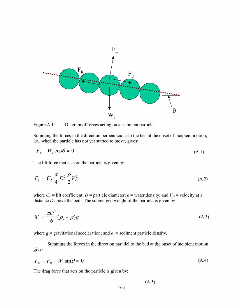
FL

2

FD FR

Ws

Figure A.1 Diagram of forces acting on a sediment particle

Summing the forces in the direction perpendicular to the bed at the onset of incipient motion, i.e., when the particle has not yet started to move, gives:

FL − Ws cosθ = 0 (A.1)

The lift force that acts on the particle is given by:

π ρFL = CL D2 VD

2 (A.2)4 2

where CL = lift coefficient; D = particle diameter; ρ = water density; and VD = velocity at a distance D above the bed. The submerged weight of the particle is given by:

πD3

Ws = (ρs − ρ)g (A.3)6

where g = gravitational acceleration; and ρs = sediment particle density.

Summing the forces in the direction parallel to the bed at the onset of incipient motion gives:

FD − FR + Ws sinθ = 0 (A.4)

The drag force that acts on the particle is given by:

(A.5) 104

π D 2 ρV 2FD = C D D4 2

where CD = drag coefficient. Yang (1973) gives the following expression for the resistance force:

FR = ψ(Ws − F L ) (A.6)

where ψ = friction coefficient.

VD in Eqs. A.2 and A.5 can be determined using a logarithmic velocity distribution:

V y y= 5.75log + B

u D* (A.7)

where Vy = velocity at a distance y above the bed; B = roughness function; and u* = (τb/ρ)0.5 = shear velocity, with τb = bed shear stress. In the hydraulically smooth regime, as defined by the shear velocity Reynolds number (given below in Eq. A.8), B is given by:

u DB = 5 5. + 5.75log *

u Dν for 0 < *

ν< 5 (A.8)

In the hydraulically rough regime, B is given by:

u DB = 8 5. for * > 70ν

Substituting y = D into Eqs. A.7 and A.8 gives VD = Bu*.

The depth-averaged velocity, V, can be obtained by integrating Eq. A.7 over the flow depth:

V ⎛ d ⎞ u*

= . ⎝⎜ D ⎠⎟ +575 log − 1 B (A.9)

Three different approaches have been used to develop criteria for incipient motion. These are the shear stress, velocity, and probabilistic approaches. The shear stress approach by Shields (1936) for determining the critical shear stress at the onset of incipient motion, τcs, is probably the most well known of all the approaches. An example of a probabilistic approach is that developed by Gessler (1965, 1970). The Shield’s shear stress approach, further developed by van Rijn (1984a), and the velocity approach used by Yang (1973) are summarized below.

The basis of the shear stress approach is that incipient motion of noncohesive sediment occurs when the bed shear stress exceeds a critical shear stress referred to as the

105

Shield’s shear stress, τcs. The latter can be defined by the following nondimensional relationship:

τθcs =

g Dcs = f R( )d (A.10) '

where gN = reduced gravitational acceleration, given by:

⎛ ρ ⎞ g' = g⎜⎜

s − 1⎟⎟ (A.11)

⎝ ρ ⎠

and Rd = sediment particle densimetric Reynolds number, given by:

D g D ' R d =

ν (A.12)

where ν = kinematic viscosity. van Rijn (1984b) gives the following expressions for f(Rd) on the right hand side of Eq. A.10:

⎧0 24 R d 2 3/ ) − for R d

/. ( 1 2 3 < 4⎪ 2 3 0 64 /⎪0. (14 R d

/ ) − . for 4 ≤ R d 2 3 < 10

f R d ) = ⎨⎪

. ( R d / ) − . for 10 ≤ R d

2 3 (A.13) ( 0 04 2 3 0 1 / < 20⎪ 2 3/ 0 .29 2 3

⎪0.013( R d ) for 20 ≤ R d / < 150

2 3⎪0.055 for R / ≥ 150⎩ d

In his velocity approach, Yang (1973) first assumed that the channel slope was small enough to neglect the component of the sediment particle’s weight in the flow direction in Eq. A.4, i.e., Wssinθ = 0. Assuming that incipient motion occurs when the two remaining terms in Eq. A.4 are equal, i.e., FD = FR, he then equated Eqs. A.5 and A.6, substituted Eq. A.9 into both sides of the resulting equation, and then solved for the dimensionless parameter Vcr/ws, where Vcr = depth-averaged critical velocity at the onset of incipient motion, and ws = particle settling velocity (i.e., terminal fall velocity). He also assumed that the drag coefficient was linearly proportional to the lift coefficient. Yang then used laboratory data sets collected by several researchers to determine the values of the friction coefficient in Eq. A.6 and the proportionality coefficient between the drag and lift coefficient to obtain the following expressions for Vcr/ws:

106

V 2 5.cr = log( ν −

+ 0.66 .

u Dw s u D * / ) 0.06 for 1 2 < *

ν< 70 (A.14)

V cr = 2.05 u Dw s for 70 ≤ * (A.15)ν

The friction force exerted along the wetted perimeter of an open channel on the flow is usually quantified using a resistance formula that contains a roughness coefficient. The Manning’s roughness coefficient is the one most commonly used for open channels with rigid boundaries. This coefficient is normally used as a calibration parameter in hydraulic models to achieve optimum agreement between measured and predicted stages (i.e., water surface elevations) or discharges. Once the model is calibrated, the Manning coefficient is treated as being temporally constant. For movable boundary problems, i.e., when sediment transport is involved, the resistance coefficient 1) will change with time due to changes in the movable bed that result from aggradation and degradation, and 2) can be attributable to two resisting forces; one force is due to the roughness of the bed surface (this is called grain roughness or skin friction), and the other force is due to the presence of bed forms in alluvial (i.e., movable boundary) channels (this is called form roughness or form drag). Einstein and Barbarossa, (1952) and other researchers have developed procedures for calculating both forms of movable boundary resistance.

The approach by Yang (1976) for estimating the grain- and form-related flow resistance in movable boundary open channels does not involve predicting what type of bed form occurs for a given flow regime (Yang, 1976). The basis for his formulation is the theory of minimum rate of energy dissipation that states that when a dynamic system (e.g., alluvial channel) reaches an equilibrium condition, its energy dissipation rate is minimum. This theory was derived from the second law of thermodynamics. The basic assumption made in this approach is that the rate of energy dissipation due to sediment transport can be neglected. For an open channel, the energy dissipation rate per unit weight of water is equal to the unit stream power VS, where V is the average flow velocity in the open channel and S is the slope of the energy grade line. Therefore, the theory of minimum energy dissipation rate requires that (Yang, 1976):

VS = V Sm m (A.16)

where the subscript m indicates the value of V and S when the unit stream power is minimized. Yang’s approach involves using Eq. A.14 or A.15 to determine the value of Vcr, and then using the following sediment transport equation developed by Yang (1973) to determine the total sediment transport:

107

logCts = 5.435 − 0.286log ws D

− 0.457 log u*

ν ws

+ ⎜⎜⎛1.799 − 0.409log

ws D − 0.314log u*

⎟⎟⎞

log⎜⎜⎛VS

− Vcr S

⎟⎟⎞

(A.17)

w⎝ ν ws ⎠ ⎝ s ws ⎠

where Cts = total sediment concentration being transported by the flow (in ppm by weight), D = median sieve diameter of the sediment, and VcrS = critical unit stream power required at incipient motion. The iterative procedure developed by Yang (1976) to determine the value of the Manning’s coefficient in an alluvial open channel uses known values for Q, D, ws, Cts, and A(d), where the latter is the functional relationship between the cross-sectional area, A, of the open channel and the flow depth, d. The Yang iterative procedure consists of the following six steps:

1. Assume a value for d = flow depth. 2. Solve the 1-D continuity equation (Q = AV) and Eq. A.17 for V and S. 3. Compute the unit stream power, i.e., VS. 4. Select another value for d and repeat steps 2 and 3. 5. Step 4 should be repeated a sufficient number of times to allow for an accurate

determination of the minimum value of VS. 6. Once the minimum value of VS has been determined, the corresponding values of V, S and d can be calculated using the 1-D continuity equation and Eq. A.17. The Manning equation (given below) can then be used to calculate the value of the Manning’s coefficient, n.

1 2 3/ 1 2 V = R S / (A.18) n where R = hydraulic radius, which is equal to the ratio A/P, where P is the wetted perimeter. Equation A.18 is the Manning’s equation form to use with metric units. Using the theory of minimum unit stream power, Yang and Song (1979) found good agreement between the following measured and computed parameters: S, V, d, VS, and n. Parker (1977) also found good agreement for flows where the sediment transport rate was not too high, thus justifying Yang’s assumption, mentioned previously, under such conditions. However, the method by Yang (1976) should not be used for critical or supercritical flows, or when the sediment transport rate is high, since the assumption is invalid under these conditions.

Immediately after onset of incipient motion, the sediment generally moves as bedload. Bedload transport occurs when noncohesive sediment rolls, slides, or jumps (i.e., saltates) along the bed. If the flow continues to increase, then some of the sediment moving as bedload will usually be entrained by vertical turbulent velocity components into the water column and be transported for extended periods of time in suspension. Thus, it takes more energy for the flow to transport sediment in suspension than as bedload. The sediment that is transported in suspension is referred to as suspended load. The total load is the sum of the bedload and suspended load. Bedload is typically between 10 - 25 percent of the total load,

108

though for beds with a high fraction of coarse sediment, the percentage will normally be higher. Many different methods have been developed for calculating the bedload transport rate in open channels. Some of these methods (along with their references) are listed next. The specific shear stress approach of van Rijn (1984a) is also described in some detail in the following.

1. Shear Stress Method: Shields (1936); Chang et al. (1967), and van Rijn (1984a). 2. Energy Slope Method: Meyer-Peter and Muller (1948). 3. Probabilistic Method: Einstein (1950)

Utilizing a shear stress approach, the dimensionless form of the bedload transport rate is given by van Rijn (1984a) as:

0 053 . = θ θ

q b . ( − )2 1

D g D R / θ . csρ ' 1 5 2 1 s d cs (A.19)

τbwhere θ =

ρg D' , qb = bedload transport rate (with units of mass per unit time per unit

width), and θcs is defined in Eq. A.10. Sediment is transported as bedload in the direction of the mean flow.

The settling velocity for individual noncohesive sediment particles, ws, is given by van Rijn (1984b) as the following functions of D, gN and Rd:

⎧ R ⎪

d for D ≤ 100μm18⎪

0 01 R − 1 1000μm (A.20) ws =⎪⎨

10 ( 1 + . d 2 ) for 100 μm< D ≤

g D ⎪ Rd ' ⎪11 . D > 1000μm ⎪⎩

To predict the noncohesive suspended sediment load in a water body, it is necessary to determine whether, for a given particle size and flow regime, the sediment is transported as bedload or as suspended load. van Rijn (1984a) presented the following approach for distinguishing between bedload and suspended load. When the bed shear velocity, u*, is less than the critical shear velocity, u*cs, no erosion is assumed to occur, and, therefore, no bedload transport occurs. Under this latter flow condition, any sediment in suspension whose critical shear velocity is greater than the bed shear velocity will deposit. When the bed shear velocity exceeds the critical shear velocity for a given particle size, erosion of that size (and smaller) sediment from the bed surface is assumed to occur. Therefore, if the following inequality is true, sediment will be transported as bedload (and not as suspended load):

109

u *cs < <u * w s (A.21)

Under this inequality condition, any suspended sediment whose critical shear velocity is greater than the bed shear velocity is assumed to deposit. If the bed shear velocity exceeds both the critical shear velocity and settling velocity for a given particle size, then that size sediment (and any smaller) is assumed to be eroded from the bed and transported as suspended load, and any sediment of that particle size (and smaller) already moving as bedload is assumed to be subsequently transported in suspension.

The rate of suspended load transport can be calculated as:

q g= ρd

ucdz (A.22) s s ∫a

where qs = suspended load transport rate per unit width of the open channel (with units of

kg/s), u = time-averaged velocity at a distance z above the bed, c = time-averaged suspended sediment concentration (by volume) at a distance z above the bed, and a = thickness of the bedload transport zone. Though not described in this report, Lane and Kalinske (1941), Einstein (1950), Brooks (1963), and Chang et al. (1965), among others, developed alternative methods to calculate qs.

The two general approaches used to calculate the total noncohesive sediment load in an open channel consist of: 1) adding the separately estimated bedload and suspended load, and 2) using a total load function that directly estimates the total amount of bedload and suspended load transport. Various formulations of the latter are briefly reviewed in this section. The advantage of using a total load approach is that sediment particles can be transported in suspension in one reach of an open channel and as bedload in another reach. In this section, only the unit stream power methods developed by Yang (1973) for estimating the total load will be presented.

The total sediment load function given by Eq. A.17 is valid for total sand concentrations less than about 100 ppm by weight. For higher sediment concentrations, Yang (1979) presented the following total load equation, again based on the unit stream power concept:

logCts = 5.165 − 0.153log ws D

− 0.297 log u*

ν ws (A.23)

⎛ ws D u* ⎞ VS+

⎝⎜⎜1.780 − 0.360log

ν− 0.480log

ws ⎠⎟⎟ log

ws

Yang (1984) also presented the following unit stream power based total load equation that is applicable for gravel sized sediment with median particle sizes between 2 and 10 mm:

110

w Ds u* (A.24) 6 681 . .log Ctg = . − 0 633 log − 4 816 log

ν ws

⎛ w Ds u* ⎞ ⎛ VS V S ⎞

⎝. − . log

ν− 0 282 . log

w ⎟ log ⎜

w −

wcr ⎟

For open channels that have bed+ ⎜ 2 784 0 305

s ⎠ ⎝ s s ⎠sediments in the sand to medium

gravel size range, i.e., between 0.063 to 10 mm, the total load would be the sum, depending on the value of Cts, of either Eqs. A.17 and A.24 or Eqs. A.23 and A.24.

When the sediment transport capacity in a given reach of an open channel exceeds the total sediment load being transported from upstream reaches, the difference between the capacity and total load is supplied from the bed. This means that the channel will undergo erosion, i.e., degradation. In a natural open channel with nonuniform bed material, the finer surficial bed sediment will be eroded more rapidly than the coarser sediment. By this process, the median diameter of the surficial bed sediment becomes coarser. If the degradation continues, the finer surficial bed sediment will eventually be depleted, leaving a layer of coarser sediment on the bed surface. This process is called armoring, and the surficial layer of coarser sediment is called the armor layer.

Garcia and Parker (1991) developed the following approach that accounts for the effect of armoring to estimate the near-bed equilibrium concentration, Ceq, for bed material that consists of multiple, noncohesive sediment size classes:

C jeq ρs

A Z(λ j )5

5 (A.25) =

⎜ 1 333A Z(λ j ) ⎞⎛ + . ⎟⎝ ⎠where Cjeq = near-bed equilibrium concentration for the j-th sediment size class, A = 1.3*10-7, and

λ 1 φ (λ − 1 (A.26) o= +σσ

φo )

u* /3 5Z = R F (A.27) j dj Hwsj

/⎛ D j ⎞

1 5

FH =⎜ ⎟⎝ D50 ⎠ (A.28)

111

where D50 = median particle size of the noncohesive bed sediments, σφ = standard deviation on the sedimentological phi scale of the bed sediment size distribution, λo = 0.81, and σφo = 0.67 (Garcia and Parker, 1991). FH is referred to as a hiding factor.

The near-bed equilibrium concentration is the suspended sediment concentration at a reference height, zeq, above the bed surface. It represents the maximum suspended sediment concentration. Some researchers take zeq to be equal to a, i.e., thickness of the bedload transport zone, in Eq. A.22. Einstein (1950) assumed that zeq = a = 2Db, where Db was defined as the representative bed sediment grain size. van Rijn (1984b) assumed zeq was equal to three grain diameters. DuBoy (1879) derived the following expression for the thickness of the bedload zone:

10( − )τ τc a = g ( )1−λ ρ ρ( − s )tan φ (A.29)

where λ = porosity of bed material, and φ = angle of repose of the bed material.

A.3.3 Cohesive sediment transport

The discussion in this section concentrates on cohesive sediment transport in estuaries. The difference between the description given here and that for cohesive sediment transport in rivers and lakes/reservoirs deals primarily with the hydrodynamics of the water bodies and the effect of salt water on the coagulation/flocculation process. The basic transport processes of erosion, advection, dispersion, settling, deposition, and consolidation are essentially the same in all types of water bodies. Thus, this brief overview of cohesive sediment transport processes in estuaries is, for the most part, relevant to all water bodies, and will provide the reader with an expanded description of sediment transport processes.

Cohesive (fine-grained) sediment transport, especially in estuaries and coastal waters, is a complex process involving a strong coupling among tides, baroclinic circulation, and the coagulated/flocculated sediment. For an extensive description of this process, the reader is referred to Postma (1967), Partheniades (1971), Barnes and Green (1971), Krone (1972), Kirby and Parker (1977), Kranck (1980) and Dyer (1986). Figure A.3 is a schematic depiction of the tidally-averaged sediment transport processes in a strongly stratified (i.e., salt wedge) estuary, e.g., Lower Duwamish Waterway, Seattle, WA. In the case of a partially mixed estuary (e.g., Charleston Harbor, SC) the description would have to be modified, i.e., there would not be a well developed salt wedge, but since relatively steep vertical density gradients are sometimes present even in such a case, the sediment transport processes would generally remain qualitatively similar to that depicted.

As indicated in Figure A.3, sediments from upstream fresh water sources arrive in the estuarial mixing zone. The high level of turbulence and the increasingly saline waters will

112

cause flocs to form and grow in size as a result of frequent interparticle collisions and increased cohesion. The large flocs will settle to the lower portion of the water column because of their high settling velocities. Results from laboratory experiments show that floc settling velocities can be up to four orders of magnitude larger than the settling velocities of

Figure A.3 Schematic representation of transport and sedimentation processes in the mixing zone of a stratified estuary (after Mehta and Hayter, 1981)

the individual particles (Bellessort 1973). Some of the sediment/flocs will deposit; the remainder will be carried upstream near the bottom until periods close to slack water when the bed shear stresses decrease sufficiently to permit deposition in the so called turbidity maximum, after which the sediment starts to undergo self-weight consolidation. The depth to which the new deposit scours when the currents increase after slack will depend on the bed shear stresses imposed by the flow and the shear strength of the deposit. Net deposition, i.e., sedimentation, will occur when the bed shear during flood, as well as during ebb, is insufficient to resuspend, i.e., erode, all of the material deposited during preceding slack periods. Some of the sediment that is resuspended may be re-entrained throughout most of the length of the mixing zone to levels above the sea water-fresh water interface, and subsequently transported downstream. At the seaward end, some material may be transported out of the estuary, a portion of which could ultimately return with the net upstream bottom current.

In the mixing zone of a typical estuary, the sediment transport rates often are an order of magnitude greater than the rate of inflow of new sediment derived from upland or oceanic sources. The estuarial sedimentary regime is characterized by several periodic (or quasi-periodic) macro-time-scales, the most important of which are the tidal period (diurnal, semi-diurnal, or mixed) and one-half the lunar month (spring-neap-spring cycle). The tidal period is the most important since it is the fundamental period that characterizes the basic mode of sediment transport in an estuary. The lunar month is often significant in determining net sedimentation rates.

113

From an Eulerian point of view, the superposition of oscillating tidal flows on the quasi-steady state transport phenomenon depicted in Figure A.3 results in corresponding oscillations of the suspended sediment concentration with time as shown in Figure A.4. Such a variation of the suspended load ultimately results from a combination of advective and dispersive transport, erosion, and deposition. Because of the complexity of the phenomenon, more than one interpretation is possible as far as any schematic representation of these phenomena is concerned. One such representation is shown in Figure A.5.

According to this description, cohesive sediments can exist in four different physical states in an estuary: mobile suspension, stationary suspension, partially consolidated bed, and settled bed. The last two are formed as a result of consolidation of a stationary suspension. Stationary here implies little horizontal movement. A stationary suspension, a partially consolidated bed and a settled bed can erode if the shear stress exceeds a certain critical value. Erosion of a stationary suspension is referred to as redispersion or mass erosion, whereas erosion of a partially consolidated bed or a settled bed is termed either resuspension or surface erosion.

To summarize, the sediment transport regime is controlled by the hydrodynamics, the chemical composition of the fluid, and the physicochemical properties of the cohesive sediments. These factors affect the processes of erosion, advection, dispersion, flocculation, settling, deposition, and consolidation. A brief description of these processes follows that of cohesive sediment beds.

A flow-deposited bed of cohesive sediment flocs possesses a vertical density and bed shear, i.e., yield, strength profile. The average values of bed density and bed shear strength increase and their vertical profiles change with time, primarily due to consolidation and secondarily due to thixotropy and associated physicochemical changes affecting inter-particle forces. Consolidation is caused by the gravitational force of overlying deposited flocs (overburden) that crushes, and thereby decreases the order of flocculation of the underlying sediment. Consolidation changes the erosive behavior of cohesive sediment beds in two ways: (1) as the shear strength of the bed increases due to consolidation, the susceptibility of the bed to erosion decreases, and (2) the vertical shear strength profile determines the depth into the bed that a bed will erode when subjected to excess shear, i.e., an applied bed shear stress in excess of the bed surface shear strength.

114

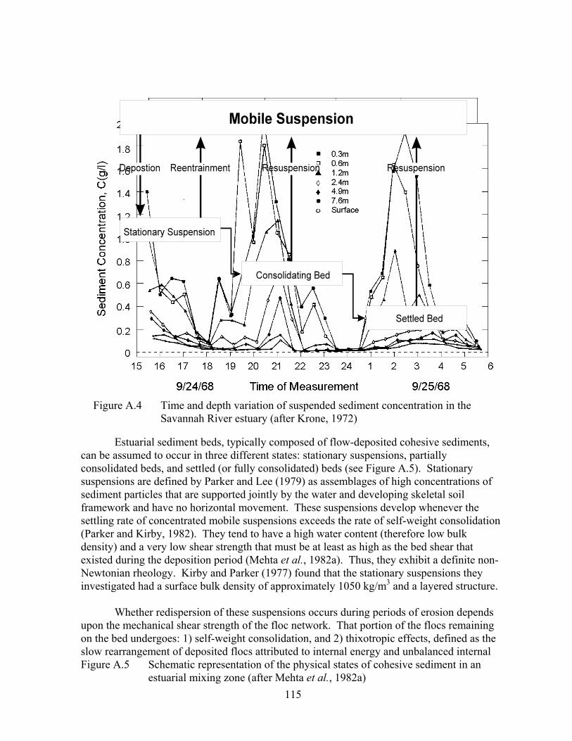
Figure A.4 Time and depth variation of suspended sediment concentration in the Savannah River estuary (after Krone, 1972)

Estuarial sediment beds, typically composed of flow-deposited cohesive sediments, can be assumed to occur in three different states: stationary suspensions, partially consolidated beds, and settled (or fully consolidated) beds (see Figure A.5). Stationary suspensions are defined by Parker and Lee (1979) as assemblages of high concentrations of sediment particles that are supported jointly by the water and developing skeletal soil framework and have no horizontal movement. These suspensions develop whenever the settling rate of concentrated mobile suspensions exceeds the rate of self-weight consolidation (Parker and Kirby, 1982). They tend to have a high water content (therefore low bulk density) and a very low shear strength that must be at least as high as the bed shear that existed during the deposition period (Mehta et al., 1982a). Thus, they exhibit a definite non-Newtonian rheology. Kirby and Parker (1977) found that the stationary suspensions they investigated had a surface bulk density of approximately 1050 kg/m3 and a layered structure.

Whether redispersion of these suspensions occurs during periods of erosion depends upon the mechanical shear strength of the floc network. That portion of the flocs remaining on the bed undergoes: 1) self-weight consolidation, and 2) thixotropic effects, defined as the slow rearrangement of deposited flocs attributed to internal energy and unbalanced internal Figure A.5 Schematic representation of the physical states of cohesive sediment in an

estuarial mixing zone (after Mehta et al., 1982a) 115

stresses (Mitchell, 1961), both of which reduce the order of flocculation of sub-surface bed layers. This implies that the bed becomes stratified with respect to density and shear strength, with both properties typically increasing monotonically with depth, at least under laboratory conditions (Mehta et al., 1982a).

Continued consolidation eventually results in the formation of settled mud, defined by Parker and Lee (1979) as “assemblages of particles predominantly supported by the effective contact stresses between particles as well as any excess pore water pressure”. This portion of the bed has a lower water content, lower order of flocculation, and higher shear strength. The settled mud in the Severn Estuary and Inner Bristol Channel, United Kingdom, was found to posses a bulk density ranging from 1300 to 1700 kg/m3 (Kirby and Parker, 1983). The nature of the density and shear strength profiles typically found in cohesive sediment beds has been revealed in laboratory tests by, among others, Richards et al. (1974), Owen (1975), Thorn and Parsons (1980), Parchure (1980), Bain (1981), Dixit (1982), and Burt and Parker (1984). A review of this subject is given by Hayter (1983).

Erosion of cohesive sediments occurs whenever the shear stress induced by water flowing over the sediment bed is great enough to break the electrochemical interparticle bonds (Partheniades, 1965; Paaswell, 1973). When this happens, erosion takes place by the removal of individual sediment particles and/or flocs. This type of erosion is time dependent and is defined as surface erosion or resuspension. In contrast, another type of erosion occurs more or less instantaneously by the removal or entrainment of relatively large pieces of the bed. This process is referred to as mass erosion or redispersion, and occurs when the flow-induced shear stresses on the bed exceed the sediment bed bulk strength along some deep-seated plane.

A number of laboratory investigations were carried out in the 1960's and 1970's in order to determine the rate of resuspension, g, defined as the mass of sediment eroded per unit bed surface area per unit time as a function of bed shear in steady, turbulent flows. An important conclusion from those tests was that the usual soil indices, such as liquid and plastic limit, do not adequately describe the erosive behavior of these sediments (Mehta, 1981). For example, Partheniades (1962) concluded that the bed shear strength as measured by standard tests, e.g., the direct-shear test (Terzaghi and Peck, 1960), has no direct relationship to the sediment's resistance to erosion that is essentially governed by the strength of the interparticle and inter-floc bonds.

The sediment composition, pore and eroding fluid compositions, and structure of the flow-deposited bed at the onset of erosion must be determined in order to properly define the erosion resistance of the bed. Sediment composition is specified by the grain size distribution of the bed material (i.e., weight fraction of clays, silts), the type of clay minerals present, and the amount and type of organic matter. The compositions of the pore and eroding fluids are specified by the temperature, pH, total amounts of salts and type and abundance of ions present, principally Cl-, Na+, Ca2+, and Mg2+. Cementing agents, such as iron oxide, can significantly increase the resistance of a sediment bed to erosion. Measurement of the

116

Ariathurai and Arulanandan (1978) found the following general relationship for the resuspension rate of consolidated beds:

⎟⎟ ⎠

⎞ ⎜⎜ ⎝

⎛ − =

c

c b M τ

τ τ ε ' (A.30)

where M' = M"τc, where M is termed the erodibility constant, τb is the flow-induced bed shear stress and τc is the bed shear strength. Values for M and τc are normally determined using either laboratory tests (Parchure, 1984), or using a device such as the SEDFLUME (McNeil et al., 1996).

electrical conductivity is used to determine the total salt concentration in the pore and eroding fluids. The effect of the bed structure, specifically the vertical sediment density and shear strength profiles, on the rate of erosion is discussed by Lambermont and Lebon (1978) and Mehta et al. (1982a).

The erosive forces, characterized by the flow-induced instantaneous bed shear stress, are determined by the flow characteristics and the surface roughness of the fluid-bed interface. Several different types of relationships between the rate of erosion, g, and the time-mean value of the flow-induced bed shear stress, τb, have been reported for non-stratified beds. These include statistical-mechanical models (Partheniades, 1965; Christensen, 1965), a rate process model (Paaswell, 1973; Kelley and Gularte, 1981), and empirical relationships (Ariathurai and Arulanandan, 1978).

Figure A.6 Relative suspended sediment concentration versus time for a stratified bed (after Mehta and Partheniades, 1979)

117

Figure A.6 shows the measured variation of C, expressed as a relative concentration by dividing the measured suspended sediment concentration by the initial suspended sediment concentration before a flow-deposited bed was formed, with time typically found by several investigators (Partheniades, 1962; Mehta and Partheniades, 1979; Mehta et al., 1982a) in laboratory resuspension tests with flow-deposited (i.e., stratified) beds under a constant τb. As observed, dC/dt is high initially, decreases monotonically with time, and appears to approach zero. The value of τc at the depth of erosion at which dC/dt, and therefore g that is proportional to dC/dt, becomes essentially zero has been interpreted to be equal to τb (Mehta et al., 1982a). This interpretation is based on the hypothesis that erosion continues as long as τb > τc. Erosion is arrested at the bed level at which τb - τc = 0. This interpretation, coupled with measurement of ρB(zb), i.e., the dry bed density profile, and the variation of C with time resulted in an empirical relationship for the rate of erosion of stratified beds. Utilizing this above approach, resuspension experiments with deposited beds were performed by Parchure (1980) in a rotating annular flume and by Dixit (1982) in a recirculating straight flume. The following empirical relationship between g and τb - τc(zb) was derived from these experiments:

ε = ε o exp⎢⎣

⎡α

τ b

τ−

c

τ (z

c

b

() zb )

⎥⎦

⎤ (A.31)

where go and α are empirical resuspension coefficients. This relationship is analogous to the rate expression that results from a heuristic interpretation of rate process theory for chemical reactions (Mehta et al., 1982a). Christensen and Das (1973), Paaswell (1973) and Kelley and Gularte (1981) have used the rate process theory in explaining the erosional behavior of cohesive sediment beds. By analogy, g is a quantitative measure of the work done by τb on the system, i.e., the bed, and go and α/τc(zb) are measures of the system's internal energy, i.e., bed resistance to an applied external force.

An important conclusion reached from these experiments was that new deposits should be treated differently from consolidated beds (Mehta et al., 1982a). The rate of surface erosion of new deposits is best evaluated using Eq. A.31, while the erosion rate for settled beds is best determined using Eq. A.30, in which g varies linearly with the normalized excess bed shear stress. The reasons for this differentiation in determining g are twofold: 1) Typical τc and ρB profiles in settled beds vary less significantly with depth than in new

τ τ 1 * deposits, and may even be nearly invariant. Therefore, the value of ( b / c )− = Δτb

will be relatively small. For Δτb * << 1 , the exponential function in Eq. A.31 can be

*⋅ + Δτ )approximated by α (1 b that represents the first two terms in the Taylor series

* *expansion of exp(α τb . Thus, for small values of Δ b⋅ Δ ) τ both expressions for g vary

linearly with Δτb * and, therefore, the variation of g with depth in settled beds can be just as

accurately and more simply determined using Eq. A.30; and 2) The laboratory resuspension tests required to evaluate the coefficients go and α for each partially consolidated bed layer

118

cannot be practically or easily performed using vertical sections of an original settled bed (obtained from cores). A simpler laboratory test has been described by Ariathurai and Arulanandan (1978) to evaluate the variability of M with depth.

Parchure and Mehta (1985) developed the following relationship for g that is applicable for soft, cohesive sediment deposits such as the top, active layer of sediment beds in estuaries:

1 2= exp[α( − ) ]ε ε τ τ

/

f b s (A.32)

where gf = floc erosion rate (gm/m2-s), τs = bed shear strength (Pa), and α = a factor that can be shown to be inversely proportional to the absolute temperature (Parchure, 1984). gf is defined to be the erosion rate when the time-averaged bed shear stress is equal to the bed shear strength, i.e., τb = τs. Even under this condition, some erosion of particles or flocs will occur due to the stochastic nature of turbulence and therefore in the instantaneous value of τb.

Sea salt is a mixture of salts, with monovalent sodium ions and divalent calcium and magnesium ions prevalent as natural electrolytes. The sodium adsorption ratio (SAR), defined as,

Na+

SAR = 1 2⎡1 (Ca2 + + Mg2 + )⎥

⎤/

⎢⎣2 ⎦ (A.33)

is a measure of the relative abundance of the three mentioned salts (cations). The cation concentrations in this equation are in milliequivalents per liter (Arulanandan, 1975). Sherard et al. (1972) have shown that the susceptibility of a cohesive sediment bed to erosion depends on two factors: 1) the pore fluid composition, as characterized by the SAR; and 2) the salinity of the eroding fluid. It was found that, as the eroding fluid salinity decreases, soil resistivity to resuspension decreases. In addition, Kandiah (1974) and Arulanandan et al. (1975) found that erosion resistance decreased and the rate of resuspension increased with increasing SAR (and therefore decreasing valency of the salt cations) of the pore fluid.

Once eroded from the bed, cohesive sediment is transported mostly as suspended load, though the author has observed clumps of cohesive sediments (i.e., mud) rolling along the bottom of both laboratory flumes and shallow rivers. The latter form of transport cannot be predicted at present. The transport of both unflocculated and flocculated cohesive sediments in suspension is the result of three processes: 1) advection - the sediment is assumed to be transported at the speed of the local mean flow; 2) turbulent diffusion - driven by spatial suspended sediment concentration gradients, the material is diffused laterally across the width of the flow channel, vertically over the depth of flow, and longitudinally in the direction of the transport; and 3) longitudinal dispersion - the suspended sediment is dispersed in the flow

119

direction by spatial velocity gradients (Ippen, 1966).

The principle of conservation of mass with appropriate source and sink terms describes the advective and dispersive transport of suspended sediment in a turbulent flow field. This principle, expressed by the advection-dispersion equation, says that the time-rate of change of mass of sediment in a stationary control volume is equated to the spatial rate of change of mass due to advection by an external flow field plus the spatial rate of change of mass due to turbulent diffusion and dispersion processes. The three-dimensional form of the advection-dispersion transport equation is:

∂C ∂C ∂C ∂C ∂ ⎡ ∂C ∂C ∂C ⎤

∂t + u

∂x + v

∂y + (w − wsc ) ∂z

=∂x ⎢⎣

Kxx ∂x + Kxy ∂y

+ Kxz ∂z ⎥⎦ (A.34)∂ ⎡ ∂C ∂C ∂C ⎤ ∂ ⎡ ∂C ∂C ∂C ⎤+∂y ⎢⎣

K yx ∂x + K yy ∂y

+ K yz ∂z ⎥⎦+

∂z ⎢⎣ Kzx ∂x

+ Kzy ∂y + Kzz ∂z ⎥⎦

+ ST

where Kij = effective sediment dispersivity tensor, and ST = the net source/sink term that accounts for source(s) (i.e., addition) of sediment to the water column due to erosion and other inputs, and sink(s) (i.e., loss) of sediment due to deposition and other removals. Implicit in this equation is the assumption that suspended material has the same velocity as the water. Sayre (1968) verified the reasonableness of this assumption for sediment particles less than about 100 μm in diameter. Rolling and saltation of sediment that occur during bed load transport can result in a significant difference between the water and sediment velocities. Therefore, the assumption of equal velocity is not applicable to bed load. The net source/sink term in Eq. A.34 can be expressed as:

+ S L d (A.35)

dC dC where is the rate of sediment addition (source) due to erosion from the bed, and dt ddt e

is the rate of sediment removal (sink) due to deposition of sediment. SL accounts for removal (sink) of a certain mass of sediment, for example, by dredging in one area (e.g., a navigational channel) of a water body, and/or dumping (source) of sediment as dredge spoil in another location.

The dispersive transport terms in Eq. A.34 include the effects of spatial velocity variations in bounded shear flows and turbulent diffusion. Thus, the effective sediment dispersivity tensor in Eq. A.34 must include the effect of all processes whose scale is less than the grid size of the model, or, in other words, what has been averaged over time and/or space (Fischer et al., 1979).

S dC dt

dC dte

= +

120

Turbulent diffusion is defined as “the transport in a given direction at a point in the flow due to the difference between the true advection in that direction and the time average of the advection in that direction,” and dispersion is defined as “the transport in a given direction due to the difference between the true advection in that direction and the spatial average of the advection in that direction” (Holley, 1969). Holley delineates the fact that diffusion and dispersion are both actually advective transport mechanisms, and that in a given flow field, the relative importance of one mechanism over the other depends on the magnitude of the concentration gradient. In Eq. A.34, the effective sediment dispersion coefficients are equal to the sum of the turbulent diffusion and dispersion coefficients. This approach follows the analysis of Aris (1956) that showed that the coefficients due to turbulent diffusion and shear flow (dispersion) were additive. Thus, analytical expressions used for the effective sediment dispersion tensor should represent both diffusion and dispersion.

Fischer (1966) showed that the dispersion of a given quantity of tracer injected into a natural stream is divided into two separate phases. The first is the convective period in which the tracer mixes vertically, laterally, and longitudinally until it is completely distributed across the stream. The second phase is the diffusive period during which the lateral, and possibly the vertical (depending on the nature of the tracer), concentration gradient is small, and the longitudinal concentration profile is highly skewed. Equation A.34 is strictly valid only in the diffusive period. The criterion for determining whether the dispersing tracer is in the diffusive period is if it has been in the flow longer than the Lagrangian time scale and has spread over a distance wider than the Lagrangian length scale (Fischer et al., 1979). The latter scale is a measure of the distance a particle travels before it forgets its initial conditions (i.e., initial position and velocity).

Analytical expressions for the sediment (mass) diffusion coefficients can be obtained by analogy with the kinematic eddy viscosity. The Reynolds analogy assumes that the processes of momentum and mass transfer are similar, and that the turbulent diffusion coefficient and the kinematic eddy viscosity, gv, are linearly proportional. Jobson and Sayre (1970) verified the Reynolds analogy for sediment particles in the Stokes range (less than about 100 μm in diameter). They found that the “portion of the turbulent mass transfer coefficient for sediment particles that is directly attributable to tangential components of turbulent velocity fluctuations: (a) is approximately proportional to the momentum transfer coefficient and the proportionality constant is less than or equal to 1; and (b) decreases with increasing particle size”. Therefore, the effective sediment mass dispersion coefficients for cohesive sediments may be justifiably assumed to be equal to those for the water itself.

Fischer et al. (1979) define four primary mechanisms of dispersion in estuaries: 1) gravitational circulation, 2) shear-flow dispersion, 3) bathymetry-induced dispersion and 4) wind-induced circulations. The last three mechanisms occur in freshwater water bodies as well. Gravitational or baroclinic circulation in estuaries is the flow induced by the density difference between freshwater at the landward end and sea water at the ocean end. There are two types of gravitational circulation. Transverse gravitational circulation is depth-averaged flow that is predominantly seaward in the shallow regions of a cross-section and landward in the deeper parts. Figure A.7a depicts this net depth-averaged upstream (landward) and

121

downstream (seaward) transport and the resulting transverse flow from the deeper to shallower parts of the cross-section. The interaction between the cross-sectional bathymetry and baroclinic flow causes the transverse circulation. Vertical gravitational circulation is schematically illustrated in Figure A.7b that also shows predominantly seaward flow in the upper part of the water column and landward flow in the lower part of the water column. Fischer (1972) said that vertical gravitational circulation is more important than transverse circulation only in highly stratified estuaries.

The mechanism of shear-flow dispersion is thought to be the dominant mechanism in long, fairly uniform sections of well-mixed and partially stratified estuaries (Fischer et al., 1979). Holley et al. (1970) concluded that for wide estuaries, the effect of the vertical velocity distribution on shear-flow dispersion is dominant over that of the transverse velocity distribution. The exact opposite situation was found for relatively narrow estuaries.

The joint influence of bathymetry and density differences on dispersion has already been mentioned in reference to baroclinic circulation. Other examples of bathymetry-induced dispersion include: intrusion of salinity or sediment into certain parts of a cross-section caused

122

(a) A Transverse Section

(b) A Vertical Section

Figure A.10 Internal circulation in a partially stratified estuary (after Fischer et al., 1979)

123

by channelization of flood and ebb tides in tidal inlets or narrow estuaries (Fischer et al., 1979), and enhanced dispersion of dissolved substances of concern (e.g., a contaminant) or intrusion of salinity into tidal flats and side embayments that then serve as storage areas for these substances, caused by the out-of-phase flow that occurs between the main channel and such features (Okubo, 1973).

An example of wind-induced circulation is shown in Figure A.8. Here, the steady onshore wind causes circulation in the wind direction in a shallow bay, where the smaller water mass per unit surface area results in a higher acceleration and, therefore, quicker response to the wind-induced surface stresses, and circulation in the opposite direction in the deeper sections of the channel. Such a circulation can cause significant dispersion (Fischer et al., 1979).

The settling rate of coagulated sediment particles depends on, in part, the size and density of the flocs, and as such is a function of the processes of coagulation and flocculation (Owen, 1970). Therefore, the factors that govern these two processes also affect the settling rate of the resulting flocs. The settling velocities of flocs can be several orders of magnitude larger than those of individual clay particles (Bellessort, 1973). For flocs from 10 to 1,000 μm in size, settling velocities have been found to range from 10-5 to 10-1 m/s (Dyer, 1989).

The following four settling zones have been identified for flocs: free settling, flocculation settling, hindered settling, and negligible settling. In the free settling zone, the settling velocities are independent of the suspension concentration. In the flocculation zone, the settling velocities increase with increasing suspension concentration due to increased interparticle collisions that result in the formation of larger and denser flocs. In the hindered settling zone, the upward transport of interstitial water is inhibited (or hindered) by the high suspension concentration. This, in turn, results in a decrease in the floc settling velocity with increasing suspension concentration. At the upper end of the hindered settling zone, the suspension concentration near the bed is so high that no settling of flocs occurs. Hwang (1989) proposed the following expressions for the floc settling velocity:

⎧w sf for C < C 1⎪ ⎪ C nw (A.36)

(C + b ) for C < C < Cw sf = ⎨a w 2 2 m w 1 3

⎪ w⎪⎩1 1. C > C 3

where wsf = free settling velocity, aw = velocity scaling coefficient, nw = flocculation settling exponent, bw = hindered settling coefficient, mw = hindered settling exponent, C1 = concentration between the free settling and flocculation settling zones, C3 = concentration at the upper limit of the hindered settling zone, and though not included in Eq. A.36, C2 = concentration between the flocculation and hindered settling zones (where wsf is maximum). Ranges of values for C1, C2, and C3 are 100 - 300 mg/L, 1,000 - 15,000 mg/L, and on the order of 75,000 mg/L, respectively (Krone, 1962; Odd and Cooper, 1989).

124

Figure A.8 Illustration of wind-induced circulation (adapted from Fischer et al., 1979)

Shrestha and Orlob (1996) developed the following expression for the settling velocity that accounts for the effect of both the suspension concentration and flow shear:

w sf = C α exp(− 4.21 + 0.147G ) (A.37)

⎛ ∂u ⎞ 2

⎛ ∂v ⎞ 2

where α = 0.11 + 0.039G , and G = ⎝⎜ ∂z ⎠⎟ + ⎝⎜ ∂z ⎠

⎟ ; i.e., G is the magnitude of the

vertical shear of the horizontal velocity.

Deposition of flocs occurs relatively quickly during slack water. Settling and deposition also occurs in slowly moving and decelerating flows, as was observed in the Savannah River Estuary (refer back to Figure A.4) during the second half of flood and ebb flows (Krone, 1972). Under these flow conditions, only those flocs with shear strengths of sufficient magnitude to withstand the highly disruptive shear stresses in the near bed region will actually deposit and adhere to the bed. Thus, deposition is governed by the bed shear stresses, turbulence structure above the bed, settling velocity, type of sediment, depth of flow, suspension concentration, and ionic constitution of the suspending fluid (Mehta and Partheniades, 1973). Specifically, deposition has been defined to occur when τb is not high enough to resuspend sediment material that settles onto and bonds with the bed surface. This process, therefore, involves two other processes, settling and bonding.

Laboratory studies on the depositional behavior of cohesive sediment in steady turbulent flows have been conducted by, among others, Krone (1962), Rosillon and Volkenborn (1964), Partheniades (1965), Lee (1974), Mehta and Partheniades (1975), Mehta et al. (1982b), Mehta and Lott (1987), Shrestha and Orlob (1996), and Teeter (2000).

125

The most commonly used expression for the sediment mass deposition rate, given initially by Einstein and Krone (1962), is:

dC w Csc ⎛⎜⎝1− b

cd

τ ⎞⎟⎠

= − dt d τ (A.38)

where τcd = critical shear stress for deposition, above which no deposition occurs. The value of τcd was found to be equal to 0.06 Pa for San Francisco Bay mud with C < 300 mg/L (Krone, 1963), and values from 0.02 to 0.2 Pa have been reported in the literature. Mehta and Lott (1987) found Eq. A.38 to agree reasonably well with laboratory data for suspended sediment concentrations up to approximately 1,000 mg/L.

A cohesive sediment bed is formed when deposited sediment particles and/or flocs comprising a stationary suspension begin to interact and form a soil that transmits an effective stress by virtue of particle-to-particle contacts. The self-weight of the particles, as well as deposition of additional material, brings the particles closer together by expulsion of pore water between the particles. A soil is formed when the water content of the sediment-water suspension decreases to the fluid limit. Unfortunately, there is not a unique water content value for cohesive soils at which the suspension changes into a soil (Been and Sills, 1981).

During the transition from suspension to soil, an extremely compressible soil framework or skeleton develops (Been and Sills, 1981). The strains involved in this first stage of consolidation are relatively large and can continue for several days or even months. The straining and upward expulsion of pore water gradually decreases as the soil skeleton continues to develop. Eventually, this skeleton reaches a state of equilibrium with the normal stress component of the overlying sediment (Parker and Lee, 1979).

During the early stages of consolidation, the self-weight of the soil mass near the bed surface is balanced by the seepage force induced by the upward flow of pore water from the underlying sediment. As the soil continues to undergo self-weight consolidation and the upward flux of pore water lessens, the self-weight of this near surface soil gradually turns into an effective stress. This surface stress and the stress throughout the soil will first crush the soil floc structure and then the flocs themselves. Primary consolidation is defined to end when the excessive pore water pressure has completely dissipated (Spangler and Handy, 1982). Secondary consolidation, that can continue for many weeks or months, is the result of plastic deformation of the soil under its overburden.

126

The shear strength of clays is due to the frictional resistance and interlocking between particles (physical component), and interparticle forces (physicochemical component) (Karcz and Shanmugam, 1974; Parchure, 1980). Consolidation results in increasing bed density and shear strength (Hanzawa and Kishida, 1981). Figure A.9 shows the increase in the shear strength profile with consolidation time and bed depth for flow-deposited kaolinite beds in tap water.

Figure A.9 Bed shear strength versus distance below the initial bed surface for various consolidation periods (after Dixit, 1982)

127

APPENDIX B

Sediment Gradation Scale (adapted from ASCE, 1975)

Sediment Class Name Size Range Size Range (mm) (μm)

Very large boulders 4096 - 2048 Large boulders 2048 - 1024

Medium boulders 1024 - 512 Small boulders 512 - 256

Large cobbles 256 - 128 Small cobbles 128 - 64

Very coarse gravel 64 - 32 Coarse gravel 32 - 16

Medium gravel 16 - 8 Fine gravel 8 - 4

Very fine gravel 4 - 2

Very coarse sand 2 - 1 2000 - 1000 Coarse sand 1 - 0.5 1000 - 500

Medium sand 0.5 - 0.25 500 - 250 Fine sand 0.25 - 0.125 250 - 125

Very fine sand 0.125 - 0.063 125 - 63

Coarse silt 0.063 - 0.031 63 - 31 Medium silt 0.031 - 0.016 31 - 16

Fine silt 0.016 - 0.008 16 - 8 Very fine silt 0.008 - 0.004 8 - 4

Coarse clay 0.004 - 0.002 4 - 2 Medium clay 0.002 - 0.001 2 - 1

Fine clay 0.001 - 0.0005 1 - 0.5 Very fine clay 0.0005 - 0.00024 0.5 - 0.24

128