“evaluation of the impact of bus rapid transit on air

Institut de Recerca en Economia Aplicada Regional i Pública Document de Treball 2015/19 1/43 Research Institute of Applied Economics Working Paper 2015/19 1/43

“Evaluation of the Impact of Bus Rapid Transit on Air Pollution”

Germà Bel and Maximilian Holst

4

WEBSITE: www.ub.edu/irea/ • CONTACT: [email protected]

The Research Institute of Applied Economics (IREA) in Barcelona was founded in 2005, as a research

institute in applied economics. Three consolidated research groups make up the institute: AQR, RISK

and GiM, and a large number of members are involved in the Institute. IREA focuses on four priority

lines of investigation: (i) the quantitative study of regional and urban economic activity and analysis of

regional and local economic policies, (ii) study of public economic activity in markets, particularly in the

fields of empirical evaluation of privatization, the regulation and competition in the markets of public

services using state of industrial economy, (iii) risk analysis in finance and insurance, and (iv) the

development of micro and macro econometrics applied for the analysis of economic activity, particularly

for quantitative evaluation of public policies.

IREA Working Papers often represent preliminary work and are circulated to encourage discussion.

Citation of such a paper should account for its provisional character. For that reason, IREA Working

Papers may not be reproduced or distributed without the written consent of the author. A revised version

may be available directly from the author.

Any opinions expressed here are those of the author(s) and not those of IREA. Research published in

this series may include views on policy, but the institute itself takes no institutional policy positions.

Abstract

Mexico City’s bus rapid transit (BRT) network, Metrobus, was introduced in an attempt to reduce congestion, increase city transport efficiency and cut air polluting emissions. In June 2005, the first BRT line in the metropolitan area began service. We use differences-in-differences and quantile regression techniques in undertaking the first quantitative policy impact assessment of the BRT system on air polluting emissions. The air pollutants considered are carbon monoxide (CO), nitrogen oxides (NOX), particulate matter of less than 2.5 µm (PM2.5), particulate matter of less than 10 µm (PM10), and sulfur dioxide (SO2). The ex-post analysis uses real field data from air quality monitoring stations for periods before and after BRT implementation. Results show that BRT constitutes an effective environmental policy, reducing emissions of CO, NOX, PM2.5 and PM10.

JEL classification: Q51, Q58, R41, R48 Keywords: Bus Rapid Transit, Differences-in-Differences, Environmental Policy Evaluation, Public Transport, Urban Air Pollution

Germà Bel: Department of Economic Policy & GiM-IREA, Universitat de Barcelona (Barcelona, Spain) ([email protected]). Maximilian Holst: Department of Economic Policy & GiM-IREA, Universitat de Barcelona (Barcelona, Spain) ([email protected]) Acknowledgements This work was supported by the Spanish Government under the project ECO2012-38004; the Catalan Government under project SGR2014-325, and the ICREA-Academia program of the Catalan Government.

1

Evaluation of the Impact of Bus Rapid Transit on Air Pollution I. Introduction

In the literature of environmental and transport economics, road transport is widely considered

one of the main sources of air pollution. More specifically, a large fraction of GHG emissions

and air pollutants are recognized as being derived from road traffic: “In 2004, transport

accounted for almost a quarter of carbon dioxide (CO2) emissions from global energy use.

Three-quarters of transport-related emissions are from road traffic” (Woodcock et al., 2009, p. 2).

Moreover, these pollution levels are particularly high in areas that suffer severe levels of traffic

congestion. Conventional road transport produces a series of pollutant emissions, which in high

concentrations represent a hazard for the inhabitants of urban areas. The most usual pollutants

are particulate matter of different size fractions (PM10 and PM2.5), carbon monoxide (CO), sulfur

dioxide (SO2), nitrogen oxides (NOX), and carbon dioxide (CO2). Combustion engines do not

necessarily produce all these pollutants, but some of the emissions from these engines in

combination with other particles in the air can react with more complex molecules (such as,

ozone) and have a negative impact on human health.

Road transit, as a major determinant of air pollution in urban areas, can be broken down

into different sectors, with one of the most relevant being that of public transport. Urban buses

emit relatively high levels of CO, NOX, PM10, and CO2. However, due to the use of cleaner, better

quality fuels and to stricter regulations on road traffic emissions, the net air quality impact of

buses can be positive if vehicles are replaced periodically. This is particularly true if cities adopt

electric vehicles and this energy is generated from renewable sources.

Public transport systems, such as subways and or light rail networks, are emission friendly

transport options that are able to transport huge numbers of people on a daily basis. The

downside of these modes of transportation, however, is the enormous initial investment they

require and the rigidity of their services. Most governments operate under considerable budget

2

constraints so that building or expanding local public transport infrastructure requires massive

investment, while construction is not always feasible owing to the nature of the local geography.

In the last few decades, governments have sought alternatives that are similarly effective

but at the same time more affordable. One such option is the Bus Rapid Transit (BRT) system, a

high-quality bus service with a similar performance to that of a subway, but provided at a fraction

of the construction cost (Cervero, 1998). Many countries around the world have adopted BRT

systems. The main factors in their favor are the low initial investment costs (especially compared

to a subway line), low maintenance costs, operating flexibility, and the fact that they provide a

rapid, reliable service (Deng & Nelson, 2011). If a BRT line is unable to capture the projected

transport demand, or if the usual route is under maintenance, the line can easily be rerouted.

The literature addressing the impact of BRT on air quality does not quantify the reduction

in concentrations of the different pollutants. Most assessments are qualitative studies of impact

effects or take the form of fuzzy cost-benefit analyses that fail to provide details about individual

pollutant levels. Our research seeks to address this gap in the literature. The contributions of this

paper are, as such, easily identifiable: a) to provide a rigorous quantification of the impact on air

quality of the introduction of a BRT network in a metropolitan area; b) to add to the few analyses

to date that employ actual field data in their evaluations of public transport policy; and c) to

employ econometric-based methods of differences-in-differences and quantile regression to

analyze the environmental impact of a public transportation system like BRT.

II. Related Literature

Several studies have examined the impact of pollutants and report the potential effects for health.

PM10 and PM2.5 have been linked with a decrease in respiratory capacity, aggravating asthmatic

conditions, and with severe heart and lung damage (WHO, 2001). Nitrogen oxides (NOX), and

particularly nitrogen dioxide (NO2), affect the respiratory system and intensify existing cases of

pneumonia or bronchitis, while NOX in high concentrations can seriously damage lung tissue.

Sulfur dioxide (SO2) can worsen existing symptoms of respiratory or cardiovascular diseases.

3

Carbon monoxide (CO) is one of the most common types of poisoning. It can disable the

transport of oxygen to the cells and cause dizziness, headaches and nausea; in high

concentrations can lead to unconsciousness and death (Neidell, 2004; Schlenker & Walker, 2011).

Moreover, PM10 is considered a risk factor for respiratory related post-neonatal mortality

and sudden infant death syndrome (Woodruff et al., 2008). The effects of alleviating traffic

congestion on infant health are analyzed extensively in Currie & Walker (2011), who show that a

reduction in congestion increases the health and development of infants significantly (see also

Kampa & Castanas, 2008; Wilhelm & Ritz, 2003; Wilhelm et al., 2008; and Lleras-Muney, 2010).

Many institutions are aware that substantial government efforts are needed to initiate

change and have accepted the challenge of fighting the problems of air pollution. And, indeed,

many governments have introduced policies to reduce the emissions generated by their services.

For example, in 2009, the São Paulo city council approved the Municipal Policy for Climate

Change, aimed at reducing GHG emissions by 20% in 2020, taking 2005 as its baseline (Lucon &

Goldemberg, 2010, p. 348). In this instance, the council’s measures focused on transportation,

renewable energy, energy efficiency, waste management, construction and land use.

Some governments have specifically targeted road traffic pollutants (World Resources

Institute, 2011). For example, in 2009, the Japanese central government announced a USD $154

billion package to foster environmentally friendly technologies. Among others, the package gives

incentives (tax breaks worth as much as $2,500) to automobile consumers for the purchase of

hybrid/electric cars, as well as subsidies of 5% on other energy efficient consumer goods. In

Germany, the government introduced low emission zones (LEZ) in many cities. Using

differences-in-differences, Wolff (2013) finds that the LEZs managed to reduce emission of PM10

by 9%.

An alternative policy for abating emissions from road traffic is the introduction of

maximum speed limits on highways or in certain metropolitan areas. Many studies have examined

the impact of such policies by employing a vast range of analytical techniques. The majority

4

calculate the impact on pollution rates resulting from changes at a local level. However, it is

implicitly assumed that no other factors play a role and, thus, the changes are summed at an

aggregate level. Moreover, the computations are often made ex-ante. In the literature, we find

Gonçalves et al. (2008), who report modest reductions of polluting emissions in Barcelona;

Keuken at al. (2010), who find a substantial reduction in polluting levels in the Netherlands; and,

Keller at al. (2008), who estimate a 4% reduction in NOX due to this policy in Switzerland.

An alternative way of evaluating the impact of a policy on pollution levels is to measure

the effect ex-post using field data. However, few studies of this type have been reported to date.

Exceptions include Bel & Rosell (2013) on the impact of an 80km/h speed limit and a variable

speed limit policy in the metro-area of Barcelona. They report that the variable speed policy was

much more effective, reducing NOX and PM10 emissions by 7.7–17.1% and 14.5–17.3%

respectively. Similarly, Van Benthem (2015) analyzed speed limits on the U.S. West Coast, and

concludes that the optimal speed, considering costs and benefits, is about 88km/h (55 mph) and

that increasing the speed would increase CO, NOX, and O2 levels. Note that Bel & Rosell (2013)

and Van Benthem (2015) use real field data; thus, they are able to measure the actual policy

impact rather than making computations based on a series of assumptions.

This paper contributes to the existing literature by providing a robust quantification of

the impact on air quality of the BRT network in a metropolitan area. We employ actual field data

in our evaluation, and use econometric-based methods of differences-in-differences and quantile

regression to analyze the environmental impact of the Bus Rapid Transit System in Mexico.

III. Bus Rapid Transit in Mexico City

Bus Rapid Transit and pollution

Bus Rapid Transit –BRT- is a relatively new mode of public transportation that has found broad

acceptance in developing countries since the early 1990s. By the end of 2014, 186 cities around

the world had adopted some form of BRT. We find prominent examples in Bogotá, Curitiba,

Guangzhou, Jakarta, and Istanbul. Latin America is seen as the epicenter of the global BRT

5

movement (Cervero, 2013) with over 60 cities using BRT, moving about 20 million people each

day; that is, 62% of the global demand for BRT services. Above all, cities in Brazil (34), Mexico

(9) and Colombia (6) have led the rapid growth of BRT networks in the region. BRT has also

developed in Europe and the U.S. Over 50 cities in Europe provide this service to an average of

2 million people daily. BRT systems exist in 18 cities in the US, transporting an average of almost

half a million people daily (see http://brtdata.org/) for figures and statistics on BRT cities).

A key feature of BRT is that it acts not only as a transport policy, but also forms part of a

country’s environmental policy. In this latter regard, it needs to be borne in mind that old buses

are being replaced by modern vehicles run on cleaner fuels, while the introduction of BRT lines

should also reduce congestion. According to Cervero (2013, p. 19), BRT is ‘likely’ to have net

benefits regarding emissions: “BRT generally emits less carbon dioxide than LRT [light rail train]

vehicles due to the use of cleaner fuels”. Cervero & Murakami (2010) consider that attracting

former motorists to BRT can reduce vehicle kilometers traveled and thus polluting emissions.

The reduction in emission levels thanks to the introduction of BRT systems is noticeable.

In Bogotá’s TransMilenio, Hidalgo et al. (2013) estimate health-cost savings from reduced

emissions following the completion of TransMilenio’s first two phases at US$114 million over a

20-year period, based on a rough computation of data. They calculate that about 8% of total

benefits can be attributed to air pollution and traffic accident savings (that is, reductions in

associated illnesses and deaths). However, the authors do not use real field data to quantify the

pollution-reduction benefits. Indeed, in Bogotá, the buses displaced by the BRT were reallocated

to the urban edge and smaller surrounding townships, leading Echeverry et al. (2005) to argue

that BRT may not have reduced the problem of polluting emissions but simply displaced it to

other areas.

Geography and Institutions

Mexico City is one of the most heavily populated metropolitan areas in the world. The estimated

population in 2005 was 19.2 million inhabitants, growing to over 20 million by 2010 (population

6

density was estimated at 2560 inhabitants/km²). The city has a subtropical highland climate and

occupies a valley at 2,220 meters above sea level. Diurnal temperatures oscillate between 10 and

22°C, and can easily climb above 30°C on hot days and fall to freezing on cold winter days.

Rainfall is intense from June to October, but it is scarce from November to May. Pollution levels

are much higher during the dry season. Wind speed plays a critical role in the city’s weather and

pollution levels: weak winds and the shape of the valley do not allow air pollutants to disperse.

The city hosts many different modes of public transport, including an extensive metro

network, light rail, buses, trolleybuses, micro-buses, taxis, etc. All modes are regulated by Mexico

City’s Mobility Secretary (SEMOVI, Mexico City Government). For several years, most modes of

public transport have operated at full capacity, resulting in lengthy commuting times, e.g., subway

commuters will typically have a long wait and have to let several trains pass before they can

board. Metro, buses and micro-buses are typically perceived as serving the lower socioeconomic

classes, as they are constantly overloaded, offer poor quality service, and due to an increasing

income gap. Those who can afford a car prefer to use it for their daily commute. Crôtte et al.

(2009) show that Mexico’s metro users that earn low wages and do not own a car perceive the

metro as a normal good, while middle/high income earners perceive the metro as inferior good.

Many bus lines serve Mexico City’s main streets and avenues. In certain cases, several bus

and micro-bus lines overlap, resulting in chaos and congestion because of the extremely slow

speeds attained and the constant stopping and starting of the bus units. Av. de los Insurgentes, one

of the longest avenues in the world at 28.8 km, and the city’s main north-to-south arterial route

used to be especially affected by congestion. The city’s public micro-bus lines suffer from an

absence of effective regulations, which means there are no official bus stops and drivers can stop

anywhere to let people on and off. The congestion attributable to the micro-buses exacerbated

commuting times. At peak hours, a commuter could take two hours to travel a distance of just 20

kilometers. This was the situation by the early 2000s, before the BRT operations were introduced.

7

The Metrobus Policy

The pollution problem is not new for Mexico City. Over the years the government tried to

implement programs aimed at reducing pollution levels. The most known one was the ‘Hoy no

circula’ (today you do not circulate) program introduced in 1989, according to which cars that do

not fulfill emission criteria could not circulate on one particular day during the week depending

on the last number of their license plate. Analyzing the impact of this program with a regression

discontinuity design, Davis (2008, p. 40) showed that this policy is not effective, but it also “led

to an increase in the total number of vehicles in circulation as well as a change in the composition

of vehicles toward high-emissions vehicles”.

On 5 November 2002, the governor of Mexico City announced an ambitious program to

deal with the worst cases of congestion. The aim was to reduce commuting times and to tackle

the city’s air quality problems, and several policies were implemented. In 2004 a few buses from

the public network were renewed. In 2006-07 some parts of the ‘second floor’ of the inner-city

highway Anillo Periférico were inaugurated. This helped reducing congestion in some areas, but the

overall amount of cars using both levels increased; so reduction of emissions was not significant.

Other minor policies were introduced in 2007, such as a pilot project of a bicycle program. All in

all, results obtained with these different programs and measures were modest.

At the heart of the 2002 program lay the introduction of a BRT (‘Metrobus’) system,

designed to reduce traffic and air pollutant emissions. The intention was not to compete with

existing public modes of transport; rather, BRT was seen as an alternative to existing options in

order to reduce congestion. Note that, as found by Anderson (2014) for Los Angeles, congestion

relief benefits alone may justify transit infrastructure investments. On March 2005, SEMOVI

oversaw the creation of the public entity Metrobus, with an initial operating budget of MXN 42.4

million pesos (USD 3.8 M in 2005). Metrobus was to be fully responsible for the BRT’s operation

planning and its control and administration.

8

The main idea underpinning the BRT system was to create an exclusive bus lane in which

only authorized buses could operate subject to certain rules and criteria (schedule time,

designated stops, physical dimensions of buses, and amount of emissions), to guarantee efficient

operation. To promote the system, several stations had to be built to enable passengers to access

the service. The project was implemented in 2005 with an initial investment of around USD $80

million to build up the infrastructure (Schipper et al., 2009). The investment included the

construction of 37 BRT stations and exclusive bus lanes and the introduction of new articulated

buses run on conventional diesel fuel. BRT was first opened on Av. de los Insurgentes; the first line

in this corridor was 19.6 km long (it was extended to 28.1 km in 2008). BRT lanes reduced traffic

congestion, as the measure eliminated overlapping of services with other bus lines. At the same

time, flow in the car lanes was improved as traffic no longer had to stop whenever a bus stopped.

Following the introduction of the Metrobus, the city’s old buses and micro-buses

operating on the same BRT route were reallocated or simply scrapped. The substitution of these

old units represented an important change in terms of the air quality conditions in the areas

adjacent to the new Metrobus route. Micro-buses, often allowed to operate because of the

authority’s negligence, represented one of the main sources of health-threatening gases for the

population. The aim of the policy was to lower the air polluting emissions of public

transportation, and the units operating the BRT network satisfy specific standards (Euro V

emission standard).

The analysis of historical trends of energy demand, air pollutants and GHG emissions

attributable to passenger vehicles commuting in Mexico City’s metro-area done by Chavez-Baeza

& Sheinbaum-Pardo (2014), reported that the primary sources of small particle matter are road

passenger transport vehicles. According to in-vehicle measurements by Shiohara et al. (2005),

carcinogenic risks caused by micro-buses were much higher than those caused by buses and the

metro. In a related study, Gómez-Perales et al. (2004) measured (in-vehicle) commuters’ exposure

to PM2.5, CO and benzene in micro-buses, buses and the metro in Mexico City during morning

9

and evening rush hours. They reported that pollution levels inside the micro-bus units presented

the highest concentrations for all the pollutants during rush hours. Wöhrnschimmel et al. (2008)

compared micro-bus, regular bus and BRT unit emissions in Mexico City. Based on in-vehicle

emission measurements, they concluded that Metrobus units were the least polluting of the three

options given that the buses are newer, more efficient and run on diesel instead of regular fuel.

While it seems intuitive that there is less pollution because of vehicle substitution, it is not

clear whether pollution levels in the metropolitan area have also been reduced. Less congestion

on a particular route may induce more people to use it. Hence, an increase in demand may even

increase pollution levels in a given area if a sufficient number of commuters are attracted to use

it. According to the Metrobus office, standard commuting times have fallen from 1 hour 30

minutes to 1 hour on the route, while passenger exposure to benzene, CO, and PM2.5 has fallen

by up to 50 percent, compared to the figures for the previous bus service operating in this

corridor. The office also claims that CO2 emissions have been cut by 35,000 tons per annum.

However, the accuracy of this information is questionable as these outcomes are likely to be

based on computations from in-vehicle emission changes, rather than real field data.

The Mexico City government monitors the air quality within its metropolitan area, by

measuring levels of various pollutants within its network of automatic air quality monitoring

stations distributed across the city. These stations have been operational during a number of

years and the information is made publicly available. We use this information to measure the

impact of the introduction of the Metrobus system on the concentrations of five pollutants.

(Insert Figure 1 around here)

The number of passengers using BRT has increased over the years, reaching satiation

point in some parts (see Table 1). Some years after the first line was opened, the network was

expanded, with lines two (20 km) and three (17 km) opening on December 2008 and February

2011, respectively. Line four (14 km) started operations on April 2012 and line five (10 km) on

November 2013. Metrobus network transported a total of 254 million passengers in 2014. The

10

Institute for Transportation and Development Policies (ITDP) evaluates BRT networks around

the world. In 2013 Mexico Metrobus was given a ‘Silver’ ranking according to the BRT Standard

Score indicating that it “includes most of the elements of international best practice and is likely

to be cost-effective on any corridor with sufficient demand to justify BRT investment. These

systems achieve high operational performance and quality of service” (BRT Standard 2014, p.10).

(Insert Table 1 around here)

IV. Data and variables

Pollution levels vary depending on a range of meteorological factors that have to be taken into

consideration to capture this variation. Air contaminants are not static and so the average daily

wind speed and average daily wind direction are included in the model. Wind direction is an

important factor as a significant amount of pollution might be created in heavily industrial areas

and then transported to other parts of the metropolitan area. Not only are pollutants transported,

they also undergo a number of reaction processes. The rates of these reactions are influenced by

temperature, so the average daily temperature needs to be considered. Water can result in a

reactive change in the equilibrium or it may increase sedimentation; thus, relative humidity and

daily rainfall are both included. Rainfall also reduces significantly the amount of pollutants in the

air and so this meteorological variable has to be included. Note, however, that owing to data

limitations, rainfall is calculated as the sum of daily rainfall amounts.

Data on air-related control variables (relative humidity, temperature, wind direction and

wind speed) were obtained from Mexico City’s Environment Secretary, which serves as the

official monitoring entity. Data on air quality and amount of polluting emissions come from the

Atmosphere Monitoring System (SIMAT), which comprises a network of around 40 monitoring

points distributed across the Mexico City metro-area. The SIMAT network is divided into four

monitoring subsystems, each measuring different atmospheric components and factors.

For the analysis of air pollutants, the RAMA (Automatic Network for Atmospheric

Monitoring) subsystem serves as the source for all pollutant measurements. The RAMA network

11

comprises 29 monitoring stations. The pollutants monitored are carbon monoxide (CO),

nitrogen oxides (NOX), sulfur dioxide (SO2), particles of the order of 10 micrometers or less in

aerodynamic diameter (PM10), and particles of the order of 2.5 micrometers or less (PM2.5).

Data on the meteorological parameters are obtained from the Meteorology and Solar

Radiation Network subsystem (REDMET), which comprises 19 continuous monitoring stations

that measure wind direction, wind speed, temperature, humidity, atmospheric pressure and solar

radiation. Unfortunately, data on atmospheric pressure and solar radiation are not available after

2003, which is a limitation of the model presented below.

Further data on rainfall were provided by Mexico City’s Water Systems office (SACM).

This network of rainfall measuring stations comprises 78 monitoring stations distributed across

the metropolitan area. Information on the exact location of the measuring stations was denied for

reasons of “national security”, given that details regarding the city’s waterworks infrastructure are

restricted access only. However, the names of the stations were provided and as these typically

include a reference to their location, it was possible with Google Maps to approximate the

location of most of them. Of the stations, 70.5% were easy to locate, 16.7% were roughly

approximated and 12.8% of the stations were impossible to locate based on their name.


As the air quality monitoring stations and rainfall measuring stations did not coincide, a

matching was undertaken. Using the location of the air quality monitoring stations the closest

rainfall station within a range of less than 10 km was selected. We assume that the weather

conditions present at the air quality stations and at their closest respective rainfall stations do not

differ. The rainfall stations that could not be located are not considered here given the

impossibility of matching them to the air quality monitoring stations (the result of the station

matching is available upon request).

Our analysis of Metrobus focuses solely on line 1 (opened on 19 June 2005). We measure

its impact for the two-year period prior to its opening and the two-year post-operational period.

12


V. Differences-in-Differences

The first part of the analysis employs the differences-in-differences method to facilitate the

measurement of the impact of the new BRT system on polluting emissions. By so doing, the

intention is to estimate the atmospheric concentration of pollutants in Mexico City between 2003

and 2007 and to assess the impact of the introduction of the Metrobus.

Methodology

The panel data used for this analysis are unbalanced. This characteristic of our panel comes from

the fact that some stations were in operation from the beginning of the period of analysis, while

other new ones were introduced at a later point in time, sometimes substituting older ones. On

the other hand, most stations required maintenance at some point. The introduction or

switching-off of the stations is exogenous and not correlated with the variables in the model.

In the absence of a randomized trial, the method adopted here is an extension of the

differences-in-differences estimation procedure specified as a two-way fixed effects model. As

stated in Wooldridg (2010: p. 828), “the usual fixed effects estimator on the unbalanced panel is

consistent”

Yit = βXit + γZit + θi + δt + εit (1)

where Yit is air pollutant concentration, Xit is a vector of time-varying control covariates that

include atmospheric characteristics, and Zit is the BRT impact dummy variable to be evaluated.

As usual in this kind of models, θi are station-specific fixed effects, δt are time-specific fixed

effects and εit is the random error. Station fixed effects control for time-invariant station-specific

omitted variables; time fixed effects control for trends around each monitoring station.

The key variable in this differences-in-differences approach is γ, which measures the

difference between the average change in air pollutant concentrations for the treatment group

(stations close to the Metrobus line) and average change in concentrations for the control group

(stations located some distance from the area through which the Metrobus passes). Specifically,

13

γ = [E(YB| BRT=1) - E(YA| BRT=1)] - [E(YB| BRT=0) - E(YA| BRT=0)] (2)

where YB and YA denote the air pollutant concentrations before and after Metrobus came into

operation. BRT=1 and BRT=0 denote treatment and control group observations respectively.

The equation for the dependent variables (CO, NOX, PM2.5, PM2.5 and SO2) is:

Yit = β0 + β1 Metrobusit + β2 Pollutant Lagit + β3 Humidityit + β4 Temperatureit + β5 Wind Directionit + β6

Wind Speedit + β7 Rainfallit + β8 Workdayt + β9 Montht + θi + δt + εit (3)

A basic assumption when using differences-in-differences is that the temporal trend in

the two areas is the same in the absence of the intervention. If this were not the case, the impact

being measured would be biased. The problem of endogeneity can also bias an impact evaluation.

According to Bertrand et al. (2004), most problems related to endogeneity can be avoided by

using the differences-in-differences technique. When using differences-in-differences in a panel

data setting, regressions must be undertaken with fixed effects: the correlation between the error

components of station i and the explanatory variables should be different from zero. Closely

related to this, an important assumption here is that unobservable variables and unobservable

characteristics remain constant over time.

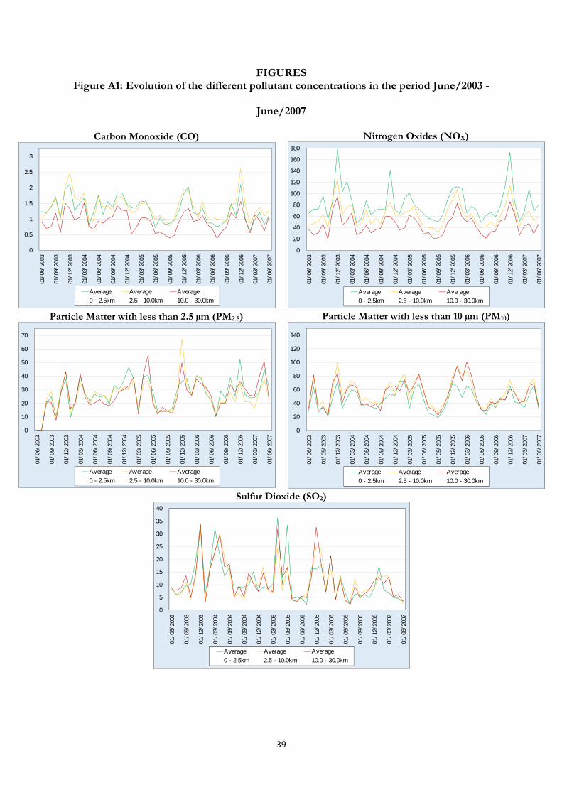
In conducting the analysis the parallel trend assumption is tested to see if the parallel

trend is satisfied in the time period before treatment (i.e. before policy implementation). For the

test, the data were grouped by trimester. The mean value of each pollutant in the treated group

(within a 2.5-km radius of the Metrobus line) was then compared with the corresponding value in

the control groups. The null hypothesis is that in the absence of intervention, the trend presented

by the treated group is equal to that presented by the control group. The null hypothesis is

accepted at the 95% confidence level, indicating that the parallel trend is satisfied for all

pollutants except for PM10. Moreover, the evolution in the pollutant levels over time is provided

in graph form in Figure A1 in the Appendix. These graphs show how the treated and the non-

treated pollutant levels behaved similarly during the pre-treatment period.

14

The failure to satisfy the parallel trend assumption in the case of PM10 leads to a biased

impact evaluation for this particular pollutant. However, despite this slightly upward bias, the

PM10 analysis is included because of the importance of this pollutant. The impact evaluation of

the remaining pollutants is not biased since the parallel trends assumption is satisfied.

As mentioned, an unbalanced panel data setting requires the use of a panel fixed effects

estimation. To confirm the correct use of fixed effects in this panel, the Hausman test was run

with every pollutant. In all cases the null hypothesis of the Hausman test was rejected at the 99%

confidence level, which confirms the correct use of the method. We test the model’s basic

assumptions (homoscedasticity, time dependence, spatial dependence and exogeneity of

explanatory variables). Autocorrelation is a persistent problem for all pollutants. To account for

this problem, we included a one-period lag of the respective pollutant in each regression.

By using Driscoll-Kraay standard errors, the estimator is modified in such a way that it is

robust to cross-section and time dependence. In this way, standard errors are also

heteroscedasticity-consistent (Driscoll & Kraay, 1998). In addition, panel-corrected standard

errors (PCSE) are used to provide a robustness analysis of the results, as PCSE yield more

accurate standard errors than estimations using feasible generalized least squares (Beck, 2001).

Results

Tables 4-8 present the results for the fixed effects regression. The models for CO, NOX, PM2.5,

PM2.5 and SO2 are all jointly statistically significant at the 1% level. All estimations include year

dummies, which capture time fixed effects (coefficients for year dummies and the constant term

are not included in the outputs, and are available upon request). R² values range between 0.59-

0.61 for CO, 0.54-0.61 for COX, 0.57-0.63 for PM2.5, 0.52-0.58 for PM10, and 0.29-0.38 for SO2.

Table 4 presents the output for the fixed effects estimation of carbon monoxide. The

estimation shows a downward trend in the relationship between the impact of the introduction of

the Metrobus on pollution and distance from the Metrobus route. In areas near the BRT line, the

reduction in concentration was 19.4%, while in the areas lying between 2.5 and 10 km and

15

between 10 and 30 km from the route the reduction was 17.2% and 16.6%, respectively. The

results also identify the influence of the time lag on current levels of carbon monoxide, i.e.,

yesterday’s pollution levels determine to a large extent today’s pollution levels. A further factor

playing a key role in the levels of CO in the air is the day of the week. Thus, pollutant levels are

much higher during the week, when workers have to commute, than on the weekends.

Environmental factors such as wind and humidity also play a marked role in air pollutant

concentrations over the city as both variables are significant.


The estimations of NOX present the opposite pattern to that presented by CO. Although

the outcome is not significant in areas close to the Metrobus route, the reduction in NOX

concentrations is greater in more distant areas. The coefficient sign is negative, which is

consistent with that of the other pollutants, and presents values between 12.2 and 18.1%. The

temporal lag plays an important role in the case of NOX, as well as in all three areas defined

around the Metrobus route. Higher wind speeds have a significant effect on the concentration

levels, blowing the pollutant into other areas when the wind speed is high. Week days have a

similar effect on pollutant concentrations as that described above for CO. For this pollutant the

year dummies are significant, capturing unobserved characteristics related to the time trend.


Table 6 presents the output of PM2.5. In this case, only seven air quality stations monitor

this pollutant within the three areas around the Metrobus route and they are not evenly

distributed. Thus, there is only one station within a 2.5-km radius of the Metrobus route, five in

the area lying between 2.5 and 10 km from the BRT line and another one in the last zone. Due to

the small number of stations, the PM2.5 regressions in the areas with just one station are estimated

with OLS using robust standard errors. Fixed effect estimations are not feasible for these areas

since the panel structure no longer holds.

16

Bearing this in mind, distance from the route has a similar impact on concentrations to

that reported above for NOX. The introduction of the Metrobus was highly significant (at the 1%

level) in bringing the concentration levels of PM2.5 down by 20.8% in the area closest to the

Metrobus line and by 39.0% in the area lying at a distance of between 10 -30 km. The temporal

lag once again is highly significant (1%), which means that the levels of concentration of this

pollutant are also largely determined by the levels the day before. The environmental factors

affecting the concentration of PM2.5 are similar to those for NOX, with the difference that

temperature plays a more important role in the area lying up to 10 km from the route. The 5%

significance of the dummy controlling for the month of the year indicates that this variable

captures significant seasonal variations within the year.


As noted, the results for PM10 present a slight upward bias and should be treated with

caution. However, the reduction in concentrations was substantial. In the area in the 2.5-km

radius of the Metrobus route, the PM10 level fell by 12.9 µg/m³ or 24.4% following the opening

of the line. The areas lying between 2.5 and 10 and between 10 and 30 km from the route had a

reduction of 17.7 and 15.5% in the levels of PM10, respectively (all reductions are statistically

significant). Table 7 shows how the impact on this pollutant fell with increasing distance from the

Metrobus; the reverse of the pattern presented by PM2.5 and NOX but the same as that of CO.


Humidity levels, wind speed and week days have an influence on PM10 concentration

levels, all three being statistically significant. Higher humidity levels reduce PM10 concentrations in

the air. Week days present higher levels of pollutant concentrations than those recorded on

weekends. In the areas lying furthest from the Metrobus route (2.5-10 km and 10-30 km), the

year dummies are significant. The temporal lag of the endogenous variable indicates that past

emission levels significantly affect today’s concentration levels. The impact of the weekday

dummy is in line with the effect on the other pollutants. Commuting to work or school at peak

17

times during the week creates congestion within the city, which increases pollution levels in areas

closest to these congested roads.

Finally, our estimations of the SO2 concentrations do not show any significant effect of

the introduction of the Metrobus in any of the three areas defined around Av. de los Insurgentes. As

expected the signs of the coefficients are negative, but the variation of the error term is too high

to capture any significant impact from the Metrobus operation. Interestingly, the model for this

pollutant performs worse in terms of explanatory power, as the coefficient of determination R² is

below that of the other pollutants. It seems probable that the model is omitting other important

determinants. As above, however, the lagged value of the endogenous variable, wind and week

day variables have a significant influence on the concentration level of SO. Higher wind speeds

reduce levels of concentration while the levels rise on days when commuters take to the roads.

The estimation outputs of the different pollutant molecules show that the introduction of

the Metrobus had a marked impact on the concentration levels of the different pollutants in the

three areas defined. To appreciate better the impact of the Metrobus operation on air quality in

the Mexico City metropolitan area, Table 9 summarizes this impact for all pollutants. In the case

of NOX and PM10 the pollutant concentration increases with distance, while in the case of CO,

PM2.5 and SO2 the concentration reduces with distance. This difference might be related to the

molecular composition of each pollutant, its molecular weight, the interaction of each pollutant

with the other molecules floating in the air, and the extent to which each pollutant is affected by

environmental factors such as wind and humidity levels.


Since estimations were carried out using Driscoll-Kraay standard errors, we also include

the results using PCSE to ensure a more robust methodological analysis. Table 9 presents the

results for the policy variable with both corrections. The policy is effective across pollutants, but

for SO2 effectiveness depends on the computation of the standard errors.


18

VI. Quantile Regression

The differences-in-differences method using fixed effects, in common with most econometric

methods, deals with the averages of distributions. This means that what is happening in different

segments of a distribution is often ignored. In order to further our analysis of the changes in air

quality following the opening of the BRT line, we divide the sample into quantiles (more

precisely, into deciles). By so doing, the analysis becomes much more detailed and we are able to

determine which deciles of the pollutants are affected most by the introduction of the Metrobus.

Quantile regression allows us to identify whether the impact concentrates around the median or,

alternatively, at the extremes of the distribution.

Methodology

The equation specified for the quantile regression resembles that specified above for the fixed

effects regression using differences-in-differences:

Q Yit (τ) = β(τ)Xit + φ(τ)Zit + θi + δt (4)

where Q Yit (τ) is the quantile function at confidence level τ. This model allows the influence of

the control variables Xit and the policy variable Zit to depend on the quantile confidence level τ.

Again, θi and δt are station-specific and time-specific fixed effects. To estimate this model,

Koenker (2004) proposes the simultaneous estimation of the following equation:

min(β, γ, θ) ∑(q=1…Q)∑ (i=1…n)∑ (t=1…T) wq ρτq (Yit - β(τ)Xit - φ(τ)Zit - θi - δt) (5)

where ρτq(·) is the function below (as in Koenker & Bassett, 1978; see also Koenker, 1984):

ρτ(u)= τ|u|, u ≥ 0 (6) (1 - τ)|u|, u < 0

The term wq are chosen weights and they control the influence of the quantiles on the

estimation of the fixed effects. Note that neither the Gaussian condition nor the classical

hypothesis related to the random error term is necessary here. Bel et al. (2015), who suggest this

way of proceeding, stress this aspect about the error term. In common with these authors, we

also assume that the weights are the same for all the quantiles analyzed. As discussed above, the

19

quantile regression expression can be seen as the differences-in-differences model decomposed

into quantiles (deciles). Therefore for any given confidence level τ,

φ = [Q(YB| BRT=1) - Q(YA| BRT=1)] - [Q(YB| BRT=0) - Q(YA| BRT=0)] (7)

where YB and YA denote the air pollutant concentrations before and after the introduction of

Metrobus. As in the first analysis, here we seek to estimate the differences between the treated air

quality monitoring stations and the stations that lie furthest away from the BRT system (control

group), while considering the changes in emissions before and after introducing Metrobus.

Recall that for the quantile regressions robust standard errors have also been used. The

robust standard errors are computed under the assumption that the residual density is continuous

and bounded away from 0 and infinity at the specified quantile (Koenker, 2005).

Results

Tables 10-12 show the results of the quantile regressions. The results of the diff-in-diff analyses

suggested that some pollutant impacts were not always significant in the three areas defined

around the Metrobus corridor. Now we determine if the areas that did not register any significant

impact on a pollutant did in fact experience some effect in some parts of the distribution.

Table 10 presents the results for the area lying closest to the Metrobus route. We obtain a

negative sign across all pollutants and deciles of the distribution. Interestingly, CO, NOX and

PM10 levels are significantly affected across the distribution, while PM2.5 shows a significant

impact in the lower deciles, becoming weaker at the upper end. SO2, which did not present

significant outcomes when using the Driscoll-Kraay standard errors, presents a significant impact

in this area at the upper end of the distribution, with the concentration level down by 63.9%.


The results for the area lying between 2.5 and 10.0 km from the line (Table 11) are

consistent with those from the differences-in-differences analysis for CO, NOX and PM2.5. In this

area, PM10 presents significant values around the median of the distribution but not at the bottom

end. This pollutant presented significant outcomes in the differences-in-differences analysis, but

20

here we see that the impact is located around the middle and upper parts of the distribution. In

common with the area adjacent to the BRT line, this area presents negative and highly significant

results for SO2. Again, when using Driscoll-Kraay standard errors this pollutant did not present

any significant results and so these results would be more in line with the PCSE estimation.


Table 12 shows the results for the area lying at a distance of between 10-30 km from the

Metrobus. This area presents very similar results to those in the second zone (2.5 to 10 km). CO,

NOX and PM2.5 are significant in all parts of the distribution while PM10 shows significant results

around the median. SO2, on the other hand, is significant around the median and at the lower

part of the distribution.


VII. Conclusions

This paper has evaluated the impact of the introduction of Bus Rapid Transit on pollution levels

in Mexico City. The analysis has been based on real field data obtained from automatic air quality

monitoring stations and has focused on five pollutants: CO, NOX, PM2.5, PM10 and SO2.

Using unbalanced panel data, we conduct an impact evaluation using the econometric-

based techniques of differences-in-differences and quantile regression, an approach not

previously used to quantify the environmental impact of this mode of transport. Results from the

differences-in-differences analysis show a significant reduction in the concentrations of all

pollutants, but SO2. Specifically, CO concentrations were reduced by 16.6-20.4%, NOX by 12.9-

18.1%, PM2.5 by 20.8-39.0% and PM10 by 9.6-24.4%, according to the city area.

In the case of SO2, the results are inconclusive. The estimation based on Driscoll-Kraay

standard errors failed to reveal any significant impact of the introduction of BRT; however, the

estimation using panel-corrected standard errors showed a significant reduction of 27.7% within

a 2.5-km radius of the Metrobus and a reduction of 23.1% in the area lying between 2.5 and 10

km from the BRT corridor.

21

The quantile regressions conducted identify the levels of the distribution at which the

policy had most impact. In the area within a 2.5-km radius of the Metrobus, the results for CO,

NOX and PM10 are significant for almost all selected quantiles of the distribution, while PM2.5 is

significant only in the lower half of the distribution (recall PM2.5 was highly significant according

to the differences-in-differences test). It is interesting to note that SO2, for which the differences-

in-differences estimation using Driscoll-Kraay standard errors showed no significance and the

estimation using PCSE revealed an impact, is significant only in the upper levels of the

distribution. However, the significance at the upper extreme is not sufficient to make the

differences-in-differences analysis with Driscoll-Kraay standard errors significant. These results

are, nevertheless, in line though with those provided by PCSE analysis.

It would be inappropriate to generalize the impact of BRT on air quality reported here to

all cities. Geographical and atmospheric traits obviously differ from one location to another.

Future research would benefit from comparing the reduction in emissions reported here with

those detected in other metropolitan areas based on real field data, and from determining

whether the latter are consistent with the findings herein. Similarly, future studies might build on

the present model and include additional environmental factors such as atmospheric pressure and

congestion monitoring variables.

For cities with similar characteristics to those of Mexico City, our results should

encourage the expansion of their BRT networks, the continuous introduction of cleaner BRT-

units, and an increase in the size of their BRT fleets to provide a better standard of service,

measures that should motivate more people to switch from private cars to public transport. It is

important to recall, however, that the emission impact of each BRT line will be different for

every corridor, and that other factors are likely to play a role. In short, decision makers that are

truly committed to the climate change fight should consider BRT as a public transport option,

and analyze whether it meets their city’s needs.

22

References

Anderson, M., 2014. Subways, Strikes, and Slowdowns: The Impacts of Public Transit on Traffic

Congestion, American Economic Review, 104, 2763–2796.

Beck, N., 2001. Time-series-cross-section data: what have we learned in the past few years?

Annual Review of Political Science, 4, 271–293.

Bel, G., Bolancé, C., Guillén, M. & Rosell, J., 2015. The environmental effects of changing speed

limits: A quantile regression approach, Transportation Research Part D, 36, 76–85.

Bel, G. & Rosell, J., 2013. Effects of the 80 km/h and variable speed limits on air pollution in the

metropolitan area of Barcelona, Transportation Research Part D, 23, 90–97.

Bertrand, M., Duflo, E. & Mullainathan, S., 2004. How much should we trust differences-in-

differences estimates? The Quarterly Journal of Economics, 119, 249-275.

Cervero, R., 1998. The transit metropolis: a global inquiry. Washington, D.C.: Island Press.

Cervero, R., 2013. Bus Rapid Transit (BRT). An efficient and competitive mode of public

transport. 20th ACEA Scientific Advisory Group Report.

Cervero, R. & Murakami, J., 2010. Effects of built Environments on vehicle miles traveled:

evidence from 370 US metropolitan areas, Environment and Planning A, 42, 400-418.

Chávez-Baeza, C. & Sheinbaum-Pardo, C., 2014. Sustainable passenger road transport scenarios

to reduce fuel consumption, air pollutants and GHG (greenhouse gas) emissions in the

Mexico City Metropolitan Area. Energy, 66, 624–634.

Crôtte, A., Noland, R. & Graham, D., 2009. Is the Mexico City metro an inferior good?, Transport

Policy, 16, 40–45.

Currie, J. & Walker, R., 2011. Traffic Congestion and Infant Health: Evidence from E-ZPass,

American Economic Journal: Applied Economics, 3, 65-90.

Davis, L., 2008. The Effect of Driving Restrictions on Air Quality in Mexico City, Journal of

Political Economy, 116, 38-81.

23

Deng, T. & Nelson, J., 2011. Recent developments in bus rapid transit: a review of the literature.

Transport Reviews, 31, 69-96.

Driscoll, J. & Kraay, A., 1998. Consistent Covariance Matrix Estimation with Spatially

Dependent Panel Data, The Review of Economics and Statistics, 80, 549-560.

Echeverry, J., Ibáñez, A., Moya, A. & Hillón, L., 2005. The Economics of Transmilenio, A Mass

Transit System for Bogotá, Economia, 5, 151–96.

Gómez-Perales, J., Colvile, R., Nieuwenhuijsen, M., Fernández-Bremauntz, A., Gutiérrez-

Avedoy, V., Páramo-Figueroa, V., Blanco-Jiménez, S., Bueno-López, E., Mandujano, F.,

Bernabé-Cabanillas, R. & Ortiz-Segovia, E., 2004. Commuters’ exposure to PM2.5, CO, and

benzene in public transport in the metropolitan area of Mexico City, Atmospheric Environment,

38, 1219–1229.

Gonçalves, M., Jiménez-Guerrero, P., López, E. & Baldasano, J., 2008. Air quality models

sensitivity to on-road traffic speed representation: effects on air quality of 80 km/h speed limit

in the Barcelona Metropolitan area, Atmospheric Environment, 42, 8389–8402.

Hidalgo, D., Pereira, L., Estupiñán, N., & Jiménez, P., 2013. TransMilenio BRT system in

Bogotá: high-performance and positive impacts; main results of an ex-post evaluation. Research

in Transportation Economics, 39, 133-138.

INEGI, 2010. Censo de población y vivienda 2010 – Estados Unidos Mexicanos Resultados Preliminares,

Instituto Nacional de Estadística y Geografía, ed.

Kampa, M. & Castanas, E., 2008. Human health effects of air pollution, Environmental Pollution,

151, 362-367.

Keller, J., Andreani-Aksoyoglu, S., Tinguely, M., Flemming, J., Heldstab, J., Keller, M., Zbinden,

R. & Prevot, A., 2008. The impact of reducing the maximum speed limit on motorways in

Switzerland to 80 km/h on emissions and peak ozone, Environmental Modelling & Software, 23,

322–332.

24

Keuken, M.P., Jonkers, S., Wilmink, I.R. & Wesseling, J., 2010. Reduced NOx and PM10

emissions on urban motorways in The Netherlands by 80 km/h speed management, Science of

the Total Environment, 408, 2517–2526.

Koenker, R., 2004. Quantile regression for longitudinal data, Journal of Multivariate Analysis, 91,

74–89.

Koenker, R., 2005. Quantile Regression, Cambridge: Cambridge University Press.

Koenker, R. & Bassett, G., 1978. Regression quantiles, Econometrica, 46, 33–50.

Lleras-Muney, A., 2010. The needs of the army: using compulsory relocation in the military to

estimate the effect of air pollutants on children's health, Journal of Human Resources, 45, 549–

590.

Lucon, O. & Goldemberg, J., 2010. São Paulo—The “Other” Brazil: Different Pathways on

Climate Change for State and Federal Governments, The Journal of Environment Development, 19,

335-357

Neidell, M., 2004. Air pollution, health, and socio-economic status: the effect of outdoor air

quality on childhood asthma, Journal of Health Economics, 23, 1209–1236.

Schlenker, W. & Walker, W., 2011. Airports, air pollution, and contemporaneous health, NBER

Working Paper, No. 17684.

Shiohara, N., Fernández-Bremauntz, A., Blanco-Jiménez, S. & Yanagisawa, Y., 2005. The

commuters’ exposure to volatile chemicals and carcinogenic risk in Mexico City, Atmospheric

Environment, 39, 3481–3489.

Van Benthem, A., 2015. What Is the Optimal Speed Limit on Freeways? Journal of Public Economics,

124, 44-62.

WHO, 2001. Quantification of health effects of exposure to air pollution. Report on a WHO Working Group.

Bilthoven, Netherlands, 20–22 November 2000. WHO Regional Office for Europe,

EUR/01/5026342 (E74256).

25

Wilhelm, M., Meng, Y., Rull, R., English, P., Balmes, J. & Ritz, B., 2008. Environmental public

health tracking of childhood asthma using California Health Interview Survey, Traffic, and

Outdoor Air Pollution Data, Environmental Health Perspectives, 116, 1254–1260.

Wilhelm, M. & Ritz, B., 2003. Residential proximity to traffic and adverse birth outcomes in Los

Angeles County, California, 1994–1996. Environmental Health Perspectives, 111, 207–216.

Wöhrnschimmel, H., Zuk, M., Martínez-Villa, G., Cerón, J., Cárdenas, B., Rojas-Bracho, L. &

Fernández-Bremauntz, A., 2007. The impact of a Bus Rapid Transit system on commuters’

exposure to Benzene, CO, PM2.5 and PM10 in Mexico City, Atmospheric Environment, 42,

8194–8203.

Wolff, H., 2013. Keep your clunker in the suburb: low-emission zones and adoption of green

vehicles, The Economic Journal, 124, F481–F512.

Woodcock, J., Edwards, P., Tonne, C., Armstrong, B., Ashiru, O., Banister, D., Beevers, S.,

Chalabi, Z., Chowdhury, Z., Cohen, A., Franco, O., Haines, A., Hickman, R., Lindsay, G.,

Mittal, I., Mohan, D., Tiwari, G., Woodward, A., Roberts, I., 2009. Health and Climate

Change 2: Public health benefits of strategies to reduce greenhouse-gas emissions: urban land

transport, The Lancet, 374, 1930-1943.

Woodruff, T., Darrow, L. & Parker, J., 2008. Air pollution and post neonatal infant mortality in

the United States, 1999–2002, Environmental Health Perspectives, 116, 110–115.

Wooldridge, J., 2010. Econometric Analysis of Cross Section and Panel Data, Massachusetts: MIT Press.

World Resources Institute, 2011. A Compilation of Green Economy Policies, Programs, and

Initiatives from Around the World. The Green Economy in Practice: Interactive Workshop 1,

February 11th, 2011.

26

FIGURES

Figure 1: Metrobus Line 1 and the air quality monitoring stations in Mexico City’s metro-area

27

TABLES

Table 1: Number of passengers using Mexico-City’s Metrobus Network

Year Line 1 Line 2 Line 3 Line 4 Line 5 Total

2005 31,515,511 0 0 0 0 34,720,301

2006 74,321,914 0 0 0 0 74,218,369

2007 77,505,395 0 0 0 0 77,652,053

2008 89,201,679 1,891,080 0 0 0 89,804,339

2009 93,455,128 33,869,530 0 0 0 127,134,909

2010 99,342,235 38,187,092 0 0 0 136,915,678

2011 113,046,246 43,469,130 32,954,167 0 0 187,183,000

2012 122,082,471 47,364,386 39,890,301 10,982,706 0 220,319,864

2013 124,891,960 48,078,130 40,546,259 13,599,680 3,157,914 230,273,943

2014 124,560,033 47,995,096 42,072,979 18,171,539 21,209,779 254,009,426

Source: Data from the Metrobus Public Information Office

28

Table 2: Description and Source of the model variables

Variable Description Source

CO Carbon Monoxide daily average concentration (ppm) RAMA

NOX Nitrogen oxides daily average concentration (ppm) RAMA

PM2.5 Particulate Matter with less than 2.5 µm (µg/m³) daily

average concentration RAMA

PM10 Particulate Matter with less than 10 µm (µg/m³) daily

average concentration RAMA

SO2 Sulfur Dioxide daily average concentration (ppm) RAMA

CO(-1), NOX(-1), PM2.5(-1),

PM10(-1), SO2(-1) One period lag (1 day) of the polluting variables RAMA

Metrobus Binary variable: 1 if the Metrobus is implemented, 0

otherwise.

Metrobus Public

Information Office

Relative humidity Daily average relative humidity (%) REDMET

Temperature Daily average temperature (°C) REDMET

Wind Direction Daily average wind direction (Azimuth Degrees) REDMET

Wind speed Daily average wind speed (m/s) REDMET

Rainfall Sum of the daily rainfall (mm) SACM

Weekdays Binary variable: 1 if the day is a labor day (Monday-

Friday), 0 if day is a Saturday or a Sunday.

Note: ppm = parts per million; µg/m³ = micrograms per cubic meter; m/s = meters per second; mm =

millimeters

29

Table 3: Descriptive statistics of the model variables

Variable Mean Std. Deviation Min. Max. Obs. Stations

CO 1.294 0.601 0.39 6.84 23.589 17

NOX 59.444 30.011 3.75 241.65 24.139 17

PM2.5 27.515 12.629 5.22 160.75 9.528 7

PM10 51.397 25.074 1.67 318.29 17.925 14

SO2 9.928 9.928 0.86 115 29.935 23

Metrobus 0.5 0.5 0 1 1.461 -

Relative humidity 56.461 12.44 24.74 87.23 16.491 18

Temperature 16.194 2.406 7.45 23.57 15.469 18

Wind Direction 186.96 23.53 116.4 295.93 16.612 17

Wind speed 1.74 0.449 0.92 3.84 16.612 17

Rainfall 1.633 2.877 0 18.88 113.958 78

Weekdays 0.714 0.452 0 1 1461 -

30

Table 4: Estimation of the logarithm of Carbon Monoxide (CO) daily average concentration

Dependent Variable: (1) (2) (3)

Log(CO) 0 - 2.5 km 2.5 - 10.0 km 10.0 - 30.0 km

Metrobus -0.1940 ** -0.1720 *** -0.1660 **

(0.0506) (0.0394) (0.0456)

Temporal lag: Log(CO) 0.5780 ** 0.5340 *** 0.5570 ***

(0.0353) (0.0217) (0.0223)

Humidity 0.0049 * 0.00381 ** 0.0060 **

(0.00206) (0.00157) (0.00193)

Temperature 0.0045 -0.0108 0.0011

(0.0123) (0.00792) (0.00966)

Wind Direction -0.0004 0.0000954 -0.0007 *

(0.000234) (0.000168) (0.000278)

Log(Wind Speed) -0.4060 *** -0.444 *** -0.4290 ***

(0.0351) (0.0344) (0.0342)

Log(Rainfall) 0.0085 -0.00125 -0.0041

(0.00502) (0.00533) (0.0063)

Workday 0.254 *** 0.211 *** 0.169 ***

(0.0186) (0.018) (0.0201)

Month -0.000382 -0.00979 -0.0135

(0.00674) (0.00537) (0.00682)

Number of Obs. 1402 2292 1555

R² 0.6546 0.5907 0.5966

Joint significance 180.00 *** 166.52 *** 151.85 ***

The regression includes a dummy for each year from 2003 to 2007 and a constant. Driscoll-Kraay

standard errors in parentheses. * p<0.10, ** p<0.05, *** p<0.01

31

Table 5: Estimation of the logarithm of Nitrogen Oxides (NOX) daily average concentration




Log(NOX) 0 - 2.5 km 2.5 - 10.0 km 10.0 - 30.0 km

Metrobus -0.1220 -0.1290 ** -0.1810 ***

(0.0545) (0.0522) (0.0449)

Temporal lag: Log(NOX) 0.4480 *** 0.3770 *** 0.4650 ***

(0.0257) (0.0199) (0.0237)

Humidity 0.0023 -0.000742 0.0036

(0.00162) (0.00103) (0.00197)

Temperature -0.0154 -0.0234 *** -0.0050

(0.00871) (0.00499) (0.0105)

Wind Direction -0.0003 -0.000083 -0.0008 **

(0.000181) (0.000124) (0.000255)

Log(Wind Speed) -0.4060 *** -0.4620 *** -0.4340 ***

(0.0339) (0.0245) (0.0322)

Log(Rainfall) -0.0014 -0.00113 -0.0071

(0.00471) (0.0045) (0.00581)

Workday 0.315 *** 0.265 *** 0.273 ***

(0.0142) (0.0146) (0.0182)

Month -0.00179 -0.00418 -0.0188 **

(0.00521) (0.00454) (0.00705)

Number of Obs. 1103 2313 1883

R² 0.6063 0.5642 0.5393


32

Table 6: Estimation of the logarithm of Particulate Matter with less than 2.5 µm (PM2.5) daily

average concentration


Log(PM2.5) 0 - 2.5 km 2.5 - 10.0 km 10.0 - 30.0 km

Metrobus -0.2080 *** -0.2530 ** -0.3900 ***

(0.0787) (0.0855) (0.096)

Temporal lag: Log(PM2.5) 0.4320 *** 0.4400 *** 0.5130 ***

(0.0447) (0.0291) (0.0507)

Humidity -0.0176 *** -0.00854 ** -0.0023

(0.00237) (0.00195) (0.00429)

Temperature -0.0261 ** 0.0087 0.0494 **

(0.0112) (0.0092) (0.0211)

Wind Direction 0.0003 0.0003540 -0.0009

(0.000495) (0.000241) (0.000791)

Log(Wind Speed) -0.5850 *** -0.5990 *** -0.5700 ***

(0.069) (0.0548) (0.0858)

Log(Rainfall) 0.0125 0.00996 0.0415 **

(0.0108) (0.00683) (0.0161)

Workday 0.120 *** 0.1240 *** 0.223 ***

(0.0305) (0.0250) -0.043

Month 0.0167 ** 0.00136 -0.0429 ***

(0.00847) (0.00695) (0.0155)

Number of Obs. 328 1416 235

R² 0.6295 0.5678 0.6205


The regression includes a dummy for each year from 2003 to 2007 and a constant. (1) & (3) use robust

standard errors and (2) uses Driscoll-Kraay standard errors. S.E. in parentheses. * p<0.10, ** p<0.05, ***

p<0.01

33

Table 7: Estimation of the logarithm of Particulate Matter with less than 10 µm (PM10) daily

average concentration


Log(PM10) 0 - 2.5 km 2.5 - 10.0 km 10.0 - 30.0 km

Metrobus -0.2440 * -0.1770 ** -0.1550 *

(0.0813) (0.0637) (0.0541)

Temporal lag: Log(PM10) 0.4390 *** 0.4410 *** 0.4670 ***

(0.0376) (0.0300) (0.0285)

Humidity -0.0125 ** -0.0137 *** -0.0166 ***

(0.0028) (0.00166) (0.00205)

Temperature 0.0142 0.0168 0.0180

(0.0107) (0.00871) (0.00865)

Wind Direction -0.0005 -0.0000011 -0.0007 *

(0.0003) (0.000167) (0.00028)

Log(Wind Speed) -0.3300 ** -0.2660 *** -0.2180 ***

(0.0526) (0.0310) (0.0361)

Log(Rainfall) 0.0188 0.0096 0.0091

(0.0074) (0.0059) (0.00648)

Workday 0.1400 ** 0.1920 *** 0.1420 ***

(0.0211) (0.0202) (0.0185)

Month 0.0093 0.00117 -0.000677

-0.0073 (0.00562) (0.00595)

Number of Obs. 1047 1643 1007

R² 0.5485 0.5248 0.5804




34

Table 8: Estimation of the logarithm of Sulfur Dioxide (SO2) daily average concentration


Log(SO2) 0 - 2.5 km 2.5 - 10.0 km 10.0 - 30.0 km

Metrobus -0.2140 -0,1760 -0,2580

(0.177) (0.173) (0.179)

Temporal lag: Log(SO2) 0.5610 *** 0,4440 *** 0,4220 ***

(0.038) (0.026) (0.0308)

Humidity -0.0027 -0,00637 * -0,0134 **

(0.00396) (0.00348) (0.00406)

Temperature -0.0006 0,0034 0,0108

(0.0198) (0.0201) (0.0213)

Wind Direction 0.0006 0,00202 *** 0,0025 ***

(0.000639) (0.000446) (0.000643)

Log(Wind Speed) -0.3760 * -0.496 *** -0,4090 ***

(0.12) (0.0795) (0.101)

Log(Rainfall) 0.0223 -0,00631 0,0120

(0.0165) (0.013) (0.0179)

Workday 0.267 ** 0,212 *** 0,143 **

(0.0513) (0.0445) (0.0551)

Month -0.00295 -0,0153 -0,0161

(0.018) (0.0133) (0.0141)

Number of Obs. 1344 2987 1867

R² 0.3849 0,3326 0,2912




35

Table 9: Summary of the impact of the Metrobus implementation on the different pollutants

(1) Less (2) Between (3) Between

than 2.5 km 2.5km - 10km 10km - 30km

CO DK -0.1940 ** -0.1720 *** -0.1660 **

(0.0506) (0.0394) (0.0456)

PCSE -0.2040 *** -0.2000 *** -0.1760 ***

(0.0426) (0.0460) (0.0473)

NOX DK -0.1220 -0.1290 ** -0.1810 ***

(0.0545) (0.0522) (0.0449)

PCSE -0.1610 *** -0.1440 *** -0.1590 ***

(0.0438) (0.0408) (0.0478)

PM2.5 DK -0.2080 *** -0.2530 ** -0.3900 ***

(0.0787) (0.0855) (0.096)

PCSE -0.2080 *** -0.2980 *** -0.3900 ***

(0.0756) (0.0602) -0.1020

PM10 DK -0.2440 * -0.1770 ** -0.1550 *

(0.0813) (0.0637) (0.0541)

PCSE -0.2160 *** -0.0960 * -0.1570 **

(0.0568) (0.0574) (0.0619)

SO2 DK -0.2140 -0.1760 -0.2580

(0.177) (0.173) (0.179)

PCSE -0.2770 ** -0.2310 ** -

(0.124) (0.116) -

Standard errors in parentheses. * p<0.10, ** p<0.05, *** p<0.01

36

Table 10: Estimated coefficients of the Metrobus implementation on the deciles of the pollutant

distributions in the area within 2.5 km around the Metrobus line 1 in Mexico-City.

Confidence Level τ (1) CO (2) NOX (3) PM2.5 (4) PM10 (5) SO2

0.90 -0.1990 *** -0.1170 * -0.3420 -0.1650 *** -0.6390 ***

(0.0443) (0.0391) (0.214) (0.0500) (0.215)

0.80 -0.1910 *** -0.1130 * -0.2620 -0.2100 *** -0.3610 ***

(0.0389) (0.0675) (0.185) (0.0412) (0.107)

0.70 -0.1830 *** -0.1040 ** -0.2350 -0.1870 *** -0.3850 ***

(0.0294) (0.0650) (0.152) (0.0486) (0.130)

0.60 -0.2080 *** -0.1100 *** -0.1730 * -0.2440 *** -0.2040

(0.0365) (0.0479) (0.0974) (0.0573) (0.128)

0.50 -0.1840 *** -0.1060 ** -0.1860 * -0.2350 *** -0.3100 **

(0.0413) (0.0447) (0.0955) (0.0504) (0.122)

0.40 -0.1830 *** -0.0941 ** -0.2270 ** -0.2560 *** -0.1710

(0.0343) (0.0385) (0.0889) (0.0567) (0.128)

0.30 -0.2190 *** -0.1020 -0.1700 -0.2090 *** -0.1880

(0.0454) (0.0418) (0.104) (0.0595) (0.166)

0.20 -0.2130 *** -0.1150 * -0.1550 ** -0.2130 *** -0.2980

(0.0443) (0.0635) (0.0716) (0.0565) (0.185)

0.10 -0.1840 *** -0.2180 *** -0.2800 *** -0.1310 * 0.0844

(0.0687) (0.0660) (0.103) (0.0713) (0.329)

Robust standard errors in parentheses. *p<0.1, **p<0.05,***p<0.01

37


distributions in the area within 2.5 and 10.0 km around the Metrobus line 1 in Mexico-City.


0.90 -0.157 *** -0.272 *** -0.342 *** -0.139 *** -0.239 **

(0.0268) (0.0725) (0.0506) (0.0251) (0.1070)

0.80 -0.207 *** -0.18 *** -0.354 *** -0.165 *** -0.311 **

(0.0385) (0.0317) (0.0638) (0.0439) (0.1440)

0.70 -0.194 *** -0.148 *** -0.275 *** -0.102 * -0.311 ***

(0.0278) (0.0491) (0.0488) (0.0557) (0.0863)

0.60 -0.197 *** -0.125 *** -0.289 *** -0.12 *** -0.343 ***

(0.0381) (0.0370) (0.0674) (0.0411) (0.0913)

0.50 -0.209 *** -0.141 *** -0.254 *** -0.169 *** -0.338 ***

(0.0353) (0.0297) (0.0543) (0.0356) (0.0808)

0.40 -0.216 *** -0.157 *** -0.276 *** -0.195 *** -0.331 ***

(0.0439) (0.0335) (0.0574) (0.0370) (0.0720)

0.30 -0.227 *** -0.14 *** -0.252 *** -0.163 *** -0.355 ***

(0.0497) (0.0378) (0.0759) (0.0381) (0.0765)

0.20 -0.184 *** -0.131 ** -0.263 *** -0.204 *** -0.229

(0.0557) (0.0606) (0.0825) (0.0701) (0.1700)

0.10 -0.152 *** -0.0921 * -0.232 *** -0.12 -0.257 **

(0.0540) (0.0522) (0.0390) (0.0745) (0.1190)


38


distributions in the area within 10.0 and 30.0 km around the Metrobus line 1 in Mexico-City.


0.90 -0.256 *** -0.187 *** -0.353 *** -0.0999 -0.147

(0.0654) (0.0546) (0.0307) (0.0983) (0.1440)

0.80 -0.171 *** -0.164 *** -0.365 *** -0.13 *** -0.313 **

(0.0564) (0.0367) (0.0610) (0.0391) (0.1390)

0.70 -0.171 *** -0.161 *** -0.281 *** -0.137 *** -0.298 ***

(0.0491) (0.0405) (0.0510) (0.0476) (0.0922)

0.60 -0.16 *** -0.166 *** -0.29 *** -0.13 ** -0.223 **

(0.0395) (0.0395) (0.0576) (0.0506) (0.0881)

0.50 -0.156 *** -0.146 *** -0.304 *** -0.151 *** -0.338 ***

(0.0427) (0.0359) (0.0488) (0.0544) (0.0783)

0.40 -0.167 *** -0.182 *** -0.281 *** -0.184 *** -0.352 ***

(0.0516) (0.0372) (0.0629) (0.0588) (0.0993)

0.30 -0.195 *** -0.191 *** -0.266 *** -0.152 ** -0.279 ***

(0.0510) (0.0411) (0.1020) (0.0622) (0.0879)

0.20 -0.145 *** -0.153 *** -0.197 ** -0.0896 -0.341 ***

(0.0532) (0.0462) (0.0818) (0.0626) (0.1200)

0.10 -0.204 *** -0.188 ** -0.319 *** -0.0892 -0.521 ***

(0.0632) (0.0773) (0.0680) (0.0692) (0.0878)


39

FIGURES Figure A1: Evolution of the different pollutant concentrations in the period June/2003 -

June/2007

Carbon Monoxide (CO) Nitrogen Oxides (NOX)

Particle Matter with less than 2.5 µm (PM2.5) Particle Matter with less than 10 µm (PM10)

Sulfur Dioxide (SO2)

0

0.5

1

1.5

2

2.5

3

01/0

6/20

03

01/0

9/20

03

01/1

2/20

03

01/0

3/20

04

01/0

6/20

04

01/0

9/20

04

01/1

2/20

04

01/0

3/20

05

01/0

6/20

05

01/0

9/20

05

01/1

2/20

05

01/0

3/20

06

01/0

6/20

06

01/0

9/20

06

01/1

2/20

06

01/0

3/20

07

01/0

6/20

07

Average

0 - 2.5km

Average

2.5 - 10.0km

Average

10.0 - 30.0km

0

20

40

60

80

100

120

140

160

180

01/0

6/20

03

01/0

9/20

03

01/1

2/20

03

01/0

3/20

04

01/0

6/20

04

01/0

9/20

04

01/1

2/20

04

01/0

3/20

05

01/0

6/20

05

01/0

9/20

05

01/1

2/20

05

01/0

3/20

06

01/0

6/20

06

01/0

9/20

06

01/1

2/20

06

01/0

3/20

07

01/0

6/20

07

Average

0 - 2.5km

Average

2.5 - 10.0km

Average

10.0 - 30.0km

0

10

20

30

40

50

60

70

01/0

6/20

03

01/0

9/20

03

01/1

2/20

03

01/0

3/20

04

01/0

6/20

04

01/0

9/20

04

01/1

2/20

04

01/0

3/20

05

01/0

6/20

05

01/0

9/20

05

01/1

2/20

05

01/0

3/20

06

01/0

6/20

06

01/0

9/20

06

01/1

2/20

06

01/0

3/20

07

01/0

6/20

07

Average

0 - 2.5km

Average

2.5 - 10.0km

Average

10.0 - 30.0km

0

20

40

60

80

100

120

140

01/0

6/20

03

01/0

9/20

03

01/1

2/20

03

01/0

3/20

04

01/0

6/20

04

01/0

9/20

04

01/1

2/20

04

01/0

3/20

05

01/0

6/20

05

01/0

9/20

05

01/1

2/20

05

01/0

3/20

06

01/0

6/20

06

01/0

9/20

06

01/1

2/20

06

01/0

3/20

07

01/0

6/20

07

Average

0 - 2.5km

Average

2.5 - 10.0km

Average

10.0 - 30.0km

0

5

10

15

20

25

30

35

40

01/0

6/20

03

01/0

9/20

03

01/1

2/20

03

01/0

3/20

04

01/0

6/20

04

01/0

9/20

04

01/1

2/20

04

01/0

3/20

05

01/0

6/20

05

01/0

9/20

05

01/1

2/20

05

01/0

3/20

06

01/0

6/20

06

01/0

9/20

06

01/1

2/20

06

01/0

3/20

07

01/0

6/20

07

Average

0 - 2.5km

Average

2.5 - 10.0km

Average

10.0 - 30.0km

Institut de Recerca en Economia Aplicada Regional i Pública Document de Treball 2014/17, pàg. 5 Research Institute of Applied Economics Working Paper 2014/17, pag. 5

“evaluation of the impact of bus rapid transit on air

Documents