evaluation of the consistency of modis land cover product
TRANSCRIPT

ISPRS Int. J. Geo-Inf. 2015, 4, 2519-2541; doi:10.3390/ijgi4042519
ISPRS International Journal of
Geo-Information ISSN 2220-9964
www.mdpi.com/journal/ijgi/
Article
Evaluation of the Consistency of MODIS Land Cover Product
(MCD12Q1) Based on Chinese 30 m GlobeLand30 Datasets: A
Case Study in Anhui Province, China
Dong Liang 1,2, Yan Zuo 1, Linsheng Huang 1,2, Jinling Zhao 1,2,*, Ling Teng 1 and Fan Yang 1
1 Key Laboratory of Intelligent Computing & Signal Processing, Ministry of Education, Anhui
University, Hefei 230039, China; E-Mails: [email protected] (D.L.); [email protected] (Y.Z.);
[email protected] (L.H.); [email protected] (L.T.); [email protected] (F.Y.) 2 Anhui Engineering Laboratory of Agro-Ecological Big Data, Anhui University, Hefei 230601, China
* Author to whom correspondence should be addressed; E-Mail: [email protected];
Tel.: +86-138-6508-1670.
Academic Editors: Emmanuel Stefanakis, Yaolin Liu, Phaedon Kyriakidis and Wolfgang Kainz
Received: 15 July 2015 / Accepted: 9 November 2015 / Published: 16 November 2015
Abstract: Land cover plays an important role in the climate and biogeochemistry of the
Earth system. It is of great significance to produce and evaluate the global land cover (GLC)
data when applying the data to the practice at a specific spatial scale. The objective of this
study is to evaluate and validate the consistency of the Moderate Resolution Imaging
Spectroradiometer (MODIS) land cover product (MCD12Q1) at a provincial scale (Anhui
Province, China) based on the Chinese 30 m GLC product (GlobeLand30). A harmonization
method is firstly used to reclassify the land cover types between five classification schemes
(International Geosphere Biosphere Programme (IGBP) global vegetation classification,
University of Maryland (UMD), MODIS-derived Leaf Area Index and Fractional
Photosynthetically Active Radiation (LAI/FPAR), MODIS-derived Net Primary Production
(NPP), and Plant Functional Type (PFT)) of MCD12Q1 and ten classes of GlobeLand30,
based on the knowledge rule (KR) and C4.5 decision tree (DT) classification algorithm. A
total of five harmonized land cover types are derived including woodland, grassland,
cropland, wetland and artificial surfaces, and four evaluation indicators are selected
including the area consistency, spatial consistency, classification accuracy and landscape
diversity in the three sub-regions of Wanbei, Wanzhong and Wannan. The results indicate
that the consistency of IGBP is the best among the five schemes of MCD12Q1 according to
the correlation coefficient (R). The “woodland” LAI/FPAR is the worst, with a spatial
OPEN ACCESS

ISPRS Int. J. Geo-Inf. 2015, 4 2520
similarity (O) of 58.17% due to the misclassification between “woodland” and “others”. The
consistency of NPP is the worst among the five schemes as the agreement varied from 1.61%
to 56.23% in the three sub-regions. Furthermore, with the biggest difference of diversity
indices between LAI/FPAR and GlobeLand30, the consistency of LAI/FPAR is the weakest.
This study provides a methodological reference for evaluating the consistency of different
GLC products derived from multi-source and multi-resolution remote sensing datasets on
various spatial scales.
Keywords: MCD12Q1; GlobeLand30; consistency evaluation; global land cover product;
Anhui Province
1. Introduction
Land use/land cover change (LUCC) is closely related to climate change, terrestrial ecosystem,
geophysical and chemical cycles, human life, etc. [1–6]. Nevertheless, it has always been a difficult
problem to derive such a parameter, especially at national, continental and even global scales, since the
emergence of remote sensing. Remote sensing technology has the ability to produce land cover products
at different spatial resolutions, especially at a global scale. Global land cover (GLC) mapping has been
given much attention by the international scientific community since the 1990s. Consequently, some
scholars have paid more attention to assessing and validating the consistency, accuracy and suitability
among different GLC products [7–12]. Meanwhile, GLC products have been distributed to the scientific
community, non-governmental organizations, individuals and governments. Therefore, it is of great
significance to evaluate and validate the quality and consistency of these GLC products [13]. At present,
several GLC products have been produced, including the International Geosphere-Biosphere Programme
Data and Information System (IGBP-DIS) DISCover of the US Geological Survey [14], University of
Maryland Land Cover Product (UMD LC) [15], CORINE of the European Commission [16,17],
Moderate Resolution Imaging Spectroradiometer (MODIS) Collection 5.1 Land Cover Type (thereafter
referred to as MCD12Q1) of Boston University [18], GLC2000 of the European Commission’s Joint
Research Centre [19], GlobCover of the European Space Agency [20,21], ECOCLIMAP of the French
Meteorological Research Center [22] and GlobeLand30 dataset of China National Basic Geographic
Information Center [23]. However, most of the developed GLC data have coarse resolutions, ranging
from 300 m to 1 km, and users generally consider it far from satisfactory due to the lack of spatial details,
low classification accuracy, and inconsistency with different products. In 2010, China launched a GLC
mapping project, and finally produced a 30 m GLC data product (GlobeLand30) with 10 classes for
years 2000 and 2010, within a four-year period.
As shown in Table 1, in comparison to other GLC products, the MODIS MCD12Q1 has an annual
updating cycle that has been updated to be more timely. Therefore, this product has an immeasurable
significance in Earth surface research and has been widely used for different applications [24–28]. The
MCD12Q1 contains five data layers, corresponding to five different classification schemes with the spatial
resolution of 500 m. Consistency analysis of MCD12Q1 has been performed in some studies [29–32].
Nevertheless, finer resolution GLC products have never been used to evaluate the product.

ISPRS Int. J. Geo-Inf. 2015, 4 2521
In this study, the GlobeLand30 and MCD12Q1 are compared by analyzing the consistency of
MCD12Q1 in Anhui Province, China by normalizing the land cover classification types between two
products based on the knowledge rule (KR) and the C4.5 decision tree (DT) classification algorithm. In
addition, the whole study area is divided into three sub-regions that have different dominant land cover
types. Four evaluation indicators of area consistency, spatial consistency, classification accuracy, and
landscape diversity indices are selected to evaluate the consistency of five land cover classification
schemes of MCD12Q1 in the three sub-regions. The novelty of this study is depicted as the following:
(1) The harmonization of land cover classification between both the GLC products is performed based
on the KR and C4.5 DT classification algorithm. A total of five land cover types are categorized from
the two datasets to evaluate the consistency of five classification schemes of MCD12Q1, specifically
including “woodland”, “grassland”, “cropland”, “wetland” and “artificial surfaces”.
(2) Three sub-regions of the study area with different spatial heterogeneities are used to evaluate the
consistency of five classification schemes of MCD12Q1 at a regional scale. The results show that the
consistency of woodland in the LAI/FPAR scheme is the worst. This can provide a methodological
reference for selecting a classification scheme from MCD12Q1 at a regional scale.
(3) It shows that the higher the landscape heterogeneity is, the larger the landscape diversity indices
are and the lower the consistency is.
Table 1. Temporal and spatial resolutions of the produced GLC products.
Dataset Available Years Spatial Resolution
IGBP-DISCover 1992–1993 1 km
UMD LC 1992–1993 1 km
CORINE 1990–2000 100 m
MCD12Q1 2001–2012 500 m
GLC2000 1999–2000 1 km
GlobCover 2005, 2009 300 m
ECOCLIMAP 1999–2005 1 km
GlobeLand30 2000, 2010 30 m
2. Study Area
Anhui Province, China, is located in the mid-latitude zone, at longitudes ranging from 114°54′E to
119°37′E and latitudes ranging from 29°41′N to 34°38′N. The province also lies in the transition zone
from alternating subtropical to temperate, with a mild and humid climate characterized by four distinct
seasons. Two major river systems—the Yangtze and the Huaihe—divide the province into the Wanbei
region, Wanzhong region and Wannan region, which form three natural areas characterized by distinctly
different geographical features (Figure 1). The Wanbei region consists of the area lying in the north of
the Huaihe River, which belongs to the North China Plain. In contrast, the Wanzhong region lies between
the Huaihe River and Yangtze River, and belongs to the agro-ecological zones of the Yangtze River
Plain. Finally, the Wannan region lies in the south of the Yangtze River, and belongs to the Tianmu
Mountains-Huaiyushan montane evergreen broadleaf ecological zone.

ISPRS Int. J. Geo-Inf. 2015, 4 2522
Figure 1. Location of Anhui Province and the Wanbei, Wanzhong and Wannan regions.
3. Data Sources and Preprocessing
The datasets utilized in this study are MCD12Q1 and GlobeLand30 (Table 2), with the former used
as the verified data and the latter as the reference data. The overall accuracy of “74.8% ± 1.3%” indicates
the accuracy ranges of the five data layers of MCD12Q1, e.g., the overall accuracy of IGBP is 74.8%.
With the best spatial resolution of 30 m, GlobeLand30 is currently considered to be the most suitable
GLC product for evaluating the consistency of MCD12Q1. In addition to these two datasets, shape
format data regarding China’s provincial administrative regions and China’s state sector datasets are
also employed.
Table 2. Comparison of the data items between MCD12Q1 and GlobeLand30.
Item MCD12Q1 GlobeLand30
Data Format HDF-EOS Geotiff
Projection Sinusoidal UTM
Total Accuracy 74.8% ± 1.3% 83.5%
Acquisition website http://reverb.echo.nasa.gov http://www.globallandcover.com

ISPRS Int. J. Geo-Inf. 2015, 4 2523
3.1. MODIS Dataset
As Table 2 shows, land cover data are obtained from MCD12Q1, a Level 3 product of the MODIS land
cover datasets. This product is derived from the MODIS output first released by the United States National
Aeronautics and Space Administration (NASA) at the end of 2008, with processed yearly observation data
from the Terra and Aqua satellites applied to depict land cover types. The chosen dataset consist of five
land cover classification systems: IGBP global vegetation classification scheme [32]; UMD vegetation
classification scheme based on the modified IGBP classification system [33]; LAI/FPAR scheme
adopted by MODIS Leaf Area Index and Fractional Photosynthetically Active Radiation (LAI/FPAR)
products (MOD15) [34,35]; NPP scheme adopted by the MODIS net primary productivity (NPP)
product (MOD17) [36]; and Plant Functional Type (PFT) land cover classification scheme [37]. In our
study, five MCD12Q1 data layers updated in 2014 are selected. The time period covered by the chosen
data range from 1 January 2010 to 31 December 2010, and the track numbers are h27v05, h27v06,
h28v05 and h28v06.
3.2. GlobeLand30 Data
Data from the American land resources satellite (Landsat) Thematic Mapper (TM5), an Enhanced
Thematic Mapper Plus (ETM+) multi spectral image, China’s Environmental Disaster Monitoring and
Forecasting Small Satellite Constellation (HJ-1A/B) and other 30 m multispectral images are applied in
the GlobeLand30 data. These data are also subsequently improved via the use of other reference data to
support processes such as sample selection and auxiliary classification. The integration of pixel- and
object-based methods with knowledge (POK) is used to control quality, which combines pixel level and
object-oriented classification [38]. The data processing is made in accordance with the order of water,
wetland, ice and snow to reduce the synonyms spectrum phenomenon, i.e., the same object has different
spectra. China donated this global 30 meters surface coverage dataset to the United Nations on
23 September 2014. This product is based on the World Geodic System (WGS) 84 coordinate system
and the Universal Transverse Mercator (UTM) projection, and comprises ten land cover types including
“water bodies”, “wetland”, “artificial surfaces”, “tundra”, “permanent snow and ice”, “grassland”,
“barren land”, “cultivated land”, “shrubland” and “forest” (Table 3). Furthermore, the overall accuracy
(OA) of GlobeLand30-2010 data is 83.50% and the Kappa coefficient (K) is 0.78. Some research on the
analysis and application of the GlobeLand30 data has been made and their results have shown good
performance [39,40]. In the present study, the GlobeLand30 product for the 2010 reference year is
selected, with the time period ranging from 1 January 2010 to 31 December 2010, and map numbers
N50_25 and N50_30.
3.3. Data Preprocessing
As the original MCD12Q1 product is stored in hierarchical data format (HDF) and with the sinusoidal
projection, data pre-processing is necessary, including format conversion, reprojection, resampling,
image mosaicking, and sub-area masking. The MODIS Reprojection Tools (MRT) professional
projection conversion system is employed for this purpose. Here, the MODIS HDF data format is
converted into Geotiff. At the same time, the data projection is converted from SIN to WGS84/UTM

ISPRS Int. J. Geo-Inf. 2015, 4 2524
and the image mosaicking and subsetting are also completed. Conversely, the acquired GlobeLand30 are
just processed by mosaicking and subsetting in ENVI 4.7 (the ENvironment for Visualizing Images
software), due to the original Geotiff format and UTM projection. Additionally, to compare the MCD12Q1
and GlobeLand30, the spatial resolution of GlobeLand30 is resampled at 500 m using the nearest neighbor
resampling method, which keeps and basically does not destroy the gray values of the original image, in
comparison with the bilinear interpolation and the cubic convolution interpolation method.
Table 3. Definitions of the ten land cover types of GlobeLand30.
Type Definition
Cultivated land Lands used for agriculture, horticulture and gardens, including paddy fields, irrigated and
dry farmlands, vegetation and fruit gardens.
Forest Lands with trees, with vegetation cover over 30%, including deciduous and coniferous
forests, and sparse woodlands with cover from 10% to 30%, etc.
Grassland Lands covered with shrubs with cover over 10%, etc.
Shrubland Land with shrubs cover over 30%, including deciduous and evergreen shrubs and deserts
steppe with cover over 10%, etc.
Wetland Lands covered with wetlands plants and water bodies, including inland marsh, lake marsh,
river floodplain wetland, forest/shrub wetland, peat bogs, mangrove and salt marsh, etc.
Water bodies Water bodies in the land area, including river, lake, reservoir and fish pond, etc.
Tundra Lands covered by lichen, moss, hardy perennial herb and shrubs in the polar regions,
including shrub tundra, herbaceous tundra, wet tundra and barren tundra, etc.
Artificial surfaces Lands modified by human activities, including the various habitation, industrial and
mining area, transportation facilities, and interior urban green zones and water bodies, etc.
Barren land Lands with vegetation cover lower than 10%, including desert, sandy fields, Gobi, bare
rocks, saline and alkaline lands, etc.
Permanent snow and ice Lands covered by permanent snow, glacier and icecap.
4. Outline and Methodology
4.1. Arrangement of Sections
To evaluate the consistency of MCD12Q1, the conceptual diagram and designed method are shown
in Figure 2. When the data sources and preprocessing are conducted in Section 3, harmonization of land
cover classification is performed based on the knowledge rule to reclassify the land cover types between
MCD12Q1 and GlobeLand30 in Section 4.2. Meanwhile, the C4.5 decision tree classification algorithm
is also introduced to finish the classification in Section 4.3. Finally, the evaluation of consistency is
performed in Section 4.4 through four indicators of area consistency (Section 4.4.1), spatial consistency
(Section 4.4.2), classification accuracy (Section 4.4.3) and landscape diversity (Section 4.4.4).
4.2. Harmonization of Land Cover Classification
A unified classification system is a necessary step when comparing different GLC products. Since
the classification schemes and categorical scales vary between MCD12Q1 and GlobeLand30, it is highly

ISPRS Int. J. Geo-Inf. 2015, 4 2525
important to reclassify the land cover categories prior to the evaluation of consistency. Hou et al.
proposed a novel method of land cover classification based on knowledge rule (KR), in which they
established the accurate LULC data by the MODIS Normalized Difference Vegetation Index (NDVI),
Digital Elevation Model (DEM) of Shuttle Radar Topography (SRTM), US Geological Survey (USGS)
classification system and two land use maps of China [41]. Ren et al. made the integration and comparison
for the IGBP, UMD, LAI/FPAR, NPP, PFT and terrestrial ecosystem features and land cover classification
schemes with six types, “farmland”, “forest”, “grassland”, “water bodies and wetland”, “settlement” and
“wilderness” [42]. Considering the land cover classification method based on KR in [41] and the
classification system in [42], the harmonization of land cover classification is performed in our study
(Table 4). A total of five land cover types are obtained including “woodland”, “grassland”, “cropland”,
“wetland” and “artificial surfaces”. In addition, there are no DN (digital number) values for the “tundra”
of GlobeLand30, and it can be removed.
Data Acquisition
C4.5 Decision Tree (DT) Classification
Algorithm
Data Preprocessing
Format Conversion
Reprojection
Image Mosaicing
Masking the Sub-regions:
Wanbei Region, Wanzhong Region and Wannan Region
Image Registration
Harmonization of Land
Cover Classification
Decision Tree Classification
Consistency Evaluation
Evaluation of Area Consistency
Analysis of Spatial Consistency
Comparison of Classification Accuracy
Assessment of Landscape Diversity
Knowledge Rule (KR) Based Categorization:
Woodland, Grassland, Cropland, Wetland
and Artificial Surfaces
MCD12Q1:
IGBP, UMD, LAI/FPAR, NPP, PFTGlobeLand30
Figure 2. Conceptual diagram and the general workflow.
Figure 3 illustrates the harmonization method of land cover classification based on KR, which is used
to harmonize the land cover classification types between the five MCD12Q1 data layers and
GlobeLand30. Firstly, the two datasets are prepared to produce the clustering center of each land cover

ISPRS Int. J. Geo-Inf. 2015, 4 2526
type. The 16-day composite MODIS NDVI dataset at a 500-m resolution of 2010 and the SRTM DEM
at a 90-m resolution provide respectively the feature space for the classification and the auxiliary
information for improving classification accuracy. Since the MCD12Q1 product has input features
comprised of the nadir BRDF-adjusted reflectance (NBAR) data, the Land Surface Temperature (LST)
data and the enhanced vegetation index (EVI) data [18]. It has the seasonal land cover region (SLCR)
characteristics, i.e., the phonological features and the first productivity in the same SLCR are the same
and they are distinctly different from those in other SLCR. In addition, the K-Means unsupervised
classification method of the multi-temporal MODIS NDVI datasets express the key classification
information and characterize the quantitative traits of each category based on SLCR. The SRTM DEM
data improve the difference between categories by the elevation data. Moreover, the phenological
variation characteristics of five MCD12Q1 data layers and GlobeLand30 form the feature vectors through
the database attribute table. These feature vectors represent the clustering centers of each category.
Subsequently, the category with the minimum Euclidean distance belongs to the corresponding land cover
type, through computing the Euclidean distance between the feature vectors of each category and the
clustering centers of each land cover type. Thus the mapping matrix is made through the mutual mapping
of different classification systems and the KR is then established as shown in Table 4. A logical look-up
table is constructed to harmonize the land cover classes. The “barren land” dose not present in Wanbei and
Wannan and dominates a very small portion of the total area, so it is ignored when evaluating the area
consistency and treated as “others”. Consequently, a total of five categories are harmonized between the
five MCD12Q1 data layers and GlobeLand30: “Woodland” is defined as the woody plant community;
“grassland” is defined as the annual or perennial herbaceous vegetation dominated by plant communities;
“cropland” is defined as the artificial cultivated vegetation cover for the purpose of the harvest; “wetland”
is defined as the surface with the saturated water for a long time in the vegetation area and the
non-vegetation area; and “artificial surfaces” refers to the lands modified by human activities.
MCD12Q1 V5.1 LCT
UMD NPPLAI/FPAR PFTIGBP
GlobeLand30-2010
Classfification Method:
Decision Tree
Clustering center
2010
MODIS
NDVI
Classification
Method:
K-Means
STRM
DEM
Elevation
Information
Minimum
Euclidean
Distance
Establishment of knolwedge rule (KR)
Clustering center
Figure 3. The flow chart of harmonizing land-cover classification based on KR.

ISPRS Int. J. Geo-Inf. 2015, 4 2527
Table 4. A total of five harmonized land cover types between MCD12Q1 and GlobeLand30.
Type IGBP UMD LAI/FPAR NPP PFT GlobeLand30
Woodland
1. Evergreen Needleleaf forest 1. Evergreen
Needleleaf forest 1. Shrubs
1. Evergreen
Needleleaf vegetation
1. Evergreen
Needleleaf trees 1. Forest
2. Evergreen Broadleaf forest 2. Evergreen
Broadleaf forest
2. Broadleaf
forest
2. Evergreen
Broadleaf vegetation
2. Evergreen
Broadleaf trees 2. Shrubland
3. Deciduous Needleleaf forest 3. Deciduous
Needleleaf forest
3. Needleleaf
forest
3. Deciduous
Needleleaf vegetation
3. Deciduous
Needleleaf trees
4. Deciduous Broadleaf forest 4. Deciduous
Broadleaf forest
4. Deciduous
Broadleaf vegetation
4. Deciduous
Broadleaf trees
5. Mixed forests 5. Mixed forests 5. Shrub
6. Closed shrublands 6. Closed
shrublands
7. Open shrublands 7. Open shrublands
Grassland
1. Woody savannas 1. Woody savannas
1.
Grasses/Cereal
crops
1. Annual Broadleaf
vegetation 1. Grass 1. Grassland
2. Savannas 2. Savannas 2. Savannas 2. Annual grass
vegetation
3. Grasslands 3. Grasslands
Cropland
1. Croplands 1. Croplands 1. Broadleaf
crops 1. Cereal crops
1. Cultivated
land
2. Croplands/Natural
vegetation
2. Broad-leaf
crops
Wetland
1. Water bodies 1. Water bodies 1. Water
bodies 1. Water bodies 1. Water bodies
1. Water
bodies
2. Permanent wetlands 2. Snow and ice 2. Wetland
3. Snow and ice 3. Permanent
snow and ice
Artificial
Surfaces 1. Urban and built-up
1. Urban and built-
up 1. Urban 1. Urban
1. Urban and
built-up
1. Artificial
Surfaces
Others 1. Barren or sparsely vegetated 1. Barren or
sparsely vegetated
1. Non-
vegetated land 1. Non-vegetated land
1. Barren or
sparse
vegetation
1. Barren land
4.3. C4.5 Decision Tree Classification
The decision tree classification technique is one of the important toolsets in data mining and has been
widely used in many fields, such as biology, computer science and technology, clinical medicine,
geology, management science and engineering [43–47]. In accordance with the top-down induction of
decision tree, a DT consists of some root nodes, which are then split into more branches [48]. The
univariate decision trees like C4.5 algorithm, using only one feature at an internal node, are the most
popular methods due to their low computational complexity [49]. In this study, we adopted the C4.5
algorithm to achieve our goal based on expert knowledge.

ISPRS Int. J. Geo-Inf. 2015, 4 2528
The classification process is divided into four steps: defining classification rules, constructing
decision tree, implementing decision tree and evaluating the classification results. Here, the
classification rules are obtained using the KR in Section 4.2 (Table 4). The new land cover types are,
respectively, extracted by the supervised decision tree operation. Specially, DT is built by the
corresponding DN values in the datasets and the classification scheme is performed in ENVI.
4.4. Evaluation of Consistency
The “consistency” is defined as the similarity characteristics of classification results for both the land
cover products. Four evaluation indicators are selected to evaluate the consistency between MCD12Q1
and GlobeLand30.
4.4.1. Area Consistency
The Pearson’s correlation coefficient (R) [50] and the percentage disagreement (PD) [51] are used to
evaluate the area consistency. Specifically, R (Equation (1)) represents the overall correlation degree
and PD (Equation (2)) represents the correlation degree on each type. It is a method of measuring the
correlation degree between two datasets and used to identify a linear correlation for a number of features
between the validated MCD12Q1 data, based on the five different classification schemes and
GlobeLand30 reference data. Similarly, the PD is used to depict the ratio of the different classification
results of the same classification type shared by the verified five data layers of MCD12Q1 and the
GlobeLand30 reference data, i.e., the degree of consistency between the two datasets. Thus, the smaller
the value of |𝑃𝐷|, the closer the results and the better the consistency.
1
2 2
1 1
(x )(y y)
100%
(x ) (y y)
n
k k
k
n n
k k
k k
x
R
x
(1)
100%k k
k k
x yPD
x y
(2)
where n is the classification number; xk and yk are, respectively, the total area of type k in MCD12Q1
and GlobeLand30; and �̅� and �̅� are, respectively, the average area of all land cover categories in
MCD12Q1 and GlobeLand30.
4.4.2. Spatial Consistency
The pixel-by-pixel comparison method is here adopted in order to verify the accuracy of spatial
positions. The spatial consistency of “woodland” is just considered in this study. First of all, the five
types of classification datasets are divided into the two categories of “woodland” and “non-woodland”
via a binarization processing method, with the five classification results of MCD12Q1 product,
respectively, superimposed with those of the GlobeLand30 product in space. Following this process,
four new types of classification data are obtained: “woodland/woodland”, “woodland/non-woodland”,
“non-woodland/woodland” and “non-woodland/non-woodland”. These new types depict the features of
ISPRS Int. J. Geo-Inf. 2015, 4 2529
the spatial consistency of “woodland” between the two datasets. Secondly, the spatial similarity of the
five MCD12Q1 classification results and those of the reference data is analyzed in the three sub-regions
and two levels (provincial and regional), as expressed by the following formula [52].
100%A
OA B C
(3)
where O is the spatial similarity coefficient, and A, B and C are, respectively, the total number of
pixels of three types of classification data: woodland/woodland, woodland/non-woodland, and
non-woodland/woodland, respectively.
4.4.3. Accuracy Verification
Accuracy verification in the present study consists of the producer accuracy (𝑝𝐴𝑖), user accuracy (𝑝𝑢𝑖) and
overall accuracy (OA) in the confusion matrix [53]. The 𝑝𝐴𝑖 is a measure indicating the probability that the
classifier has labeled an image pixel into Class i given that the ground truth is Class i. (Equation (4)). The
𝑝𝑢𝑖 is a measure indicating the probability that a pixel is Class i given that the classifier has labeled the
pixel into Class i (Equation (5)). The OA is calculated by summing the number of pixels classified
correctly and dividing by the total number of pixels (Equation (6)). The formulas used to calculate the
𝑝𝐴𝑖, 𝑝𝑢𝑖 and OA are as follows:
A /i ii ip p p (4)
/iu ii ip p p (5)
1
/n
ii
i
OA p p
(6)
The Kappa coefficient (K) measures data coincidence via a discrete multivariate technique [54].
Moreover, considering the possibility of accidental consistency between two groups of data sets, the K
reflects the classification accuracy of land cover products more exactly (Equation (7)).
1 1
2
1
( )
( )
r r
ii i i
i i
r
i i
i
N p p p
K
N p p
(7)
where pii is the constituents in which the type i of the classification results of MCD12Q1 is consistent
with the type i of GlobeLand30, i.e., the number of the correctly classified pixels; P is the sum of all
pixels in the GlobeLand30 classification result; pi+ is the sum of the type i in the classification result of
MCD12Q1 in line i; p+i is the sum of the type i in the classification result of GlobeLand30 in column i;
and N is the number of the pixels used for the accuracy evaluation.
4.4.4. Landscape Diversity
In the present paper, two landscape diversity indices are selected [55], including the modified
Simpson’s diversity index (MSIDI) (Equation (8)) and the modified Simpson’s evenness index (MSIEI)
(Equation (9)), in order to analyze the characteristics of the landscape mosaic. The landscape diversity
ISPRS Int. J. Geo-Inf. 2015, 4 2530
indices of both the five MCD12Q1 layers and the GlobeLand30 are measured and compared. MSIDI is
applied for calculating the ecological community and landscape diversity, with the stronger sensitivity
for rare patch types. MSIEI, as a supplement of patch dominance, reflects the equilibrium ratios of the
area proportions of different patch types and their maximum values in the landscape. The classification
results of the MCD12Q1 and GlobeLand30 products are recorded in 8-bit unsigned integer format using
the Fragstats 4.2 software program. The diversity index shows the species diversity of animals and plants
in an area and is widely used in landscape ecology. Diversity index values are mainly affected by the
richness and evenness of landscape composition, which, respectively, illustrate the diversity of landscape
composition and landscape structure. In the present study, the landscape diversity metric in Fragstats is
applied for the comparison of the Wanbei, Wanzhong and Wannan regions. The Simpson’s diversity
index is based on the establishment of information theory, in view of the measurement of biological
communities. A widely applied method, Simpson’s diversity index values represent the probability that
two randomly selected grid units belong to different patch types.
The MSIDI is expressed by
2
1
lnm
i
i
MSIDI p
(8)
The MSIEI is given by
2
1
ln
ln
m
i
i
p
MSIEIm
(9)
where pi is the area proportion of patch type i in the landscape, with the total area of the landscape not
including background values; and m is the number of patch types in the landscape. All these indicators
have no units. Index value ranges are MSIDI ≥ 0 and 0 ≤ MSIEI ≤ 1. When the whole landscape contains
only one patch, MSIDI = 0 and MSIEI = 0. With an increasing number of landscape patches and the
continuous equalization of their area proportions, the value of MSIDI increases. When the proportion of
each patch in the landscape is the same, MSIEI = 1. With a more and more unbalanced proportion of
different patch types in the landscape, the values of MSIEI approach zero.
5. Results and Discussion
5.1. Validation of Classification Accuracy of GlobeLand30
Since GlobeLand30 data are used as the reference data, it is highly necessary to firstly evaluate the
classification accuracy for ensuring the reliability. The statistics of primary land cover types are selected,
including the crop and forest area from the Anhui Statistical Yearbook [56] and the wetland area from
the second China wetland survey [57]. The fractional error is used to validate the accuracy of
GlobeLand30, which represents a ratio of the absolute value of the differences between the actual area
and estimated area and the actual area.
As shown in Table 5, in addition to the “woodland” in Wanbei and “wetland” in Wanbei and Wannan,
all the other fractional errors are less than 30%. Furthermore, “woodland” is taken as a study case to
compare the MCD12Q1 and GlobeLand30. The “woodland” area derived from the five classification

ISPRS Int. J. Geo-Inf. 2015, 4 2531
schemes of MCD12Q1 is, respectively, 42.75 km2 of IGBP, 53.50 km2 of UMD, 8.75 km2 of LAI/FPAR,
52.75 km2 of NPP and 57.00 km2 of PFT in Wanbei, while it is 106.25 km2 of GlobeLand30 and is much
closer to the yearbook statistics. Therefore, the GlobeLand30 have higher classification accuracy and
can be used as the reference data for evaluating the consistency of MCD12Q1.
Table 5. Accuracy validation for “woodland”, “cropland” and “wetland” of GlobeLand30.
Region Land Cover Type Area (km2) Yearbook Statistics Fractional Error (%)
Anhui Province
Woodland 36711.25 38042.20 3.50
Cropland 82294.50 90865.91 9.43
Wetland 7346.50 10418.00 29.48
Wanbei
Woodland 106.25 5628.60 98.11
Cropland 25786.00 35316.03 26.98
Wetland 326.00 1230.47 73.51
Wanzhong
Woodland 15549.50 14104.50 10.24
Cropland 44284.50 45209.74 2.05
Wetland 5610.25 6271.95 10.55
Wannan
Woodland 21056.75 18309.10 15.01
Cropland 12239.50 10340.14 18.37
Wetland 1416.00 2915.58 51.43
5.2. Evaluation of Area Consistency
Table 6 compares the R values of IGBP, UMD, LAI/FPAR, NPP and PFT in Wanbei, Wanzhong,
Wannan and Anhui Province, respectively. Significantly, all the R values of IGBP, UMD and PFT are
more than 97% in the three sub-regions. Their consistency shows pretty good on the whole. Considering
the R values vary slightly from 98.22% to 99.61% in the three sub-regions and the whole Anhui Province,
the compatibility and robustness of IGBP is best, indicating that the consistency of IGBP is best on a
regional scale. The obtained result is the same with the reference [42], which shows that the area of land
cover types of IGBP are more close to the land cover classification schemes based on the terrestrial
ecosystem features and remote sensing (TEFRS).
On the other hand, the R of LAI/FPAR and NPP has poor performance, which shows that the regional
variation is obvious. For the LAI/FPAR, the R decreases from 56.40% of Wannan to −17.78% of
Wanbei. The R of the NPP scheme varies from −31.47% of Wanbei to 69.26% of Wannan. To analyze
the high regional variation of LAI/FPAR and NPP, PD is used to provide the correlation degree on each
type in the five schemes. Combining the R and PD, more detailed consistency evaluation of the five
schemes can be presented.
Figure 4 shows the comparison of area consistency of five types derived from the five schemes. As shown
in blue and orange columns, the PD of IGBP and UMD are smaller than that of the other three schemes on
each type in the three sub-regions, showing their consistency are better. The “woodland” and “grassland”
(orange column) in the three sub-regions show particularly the best performance among the five schemes,
which highlights that the consistency of UMD is best for “woodland” and “grassland”. The study [58] shows
the same result that UMD is best to reflect the temporal and spatial distribution of grassland.

ISPRS Int. J. Geo-Inf. 2015, 4 2532
The grey column illustrates the PD of LAI/FPAR and it shows that the classification results of
“woodland” in the three sub-regions are worst among the five schemes, particularly in Wanbei with less
forest resources. The result is also similar with the conclusion of the reference [58]. Moreover, the
consistency of “artificial surfaces” in the three sub-regions is also worst among the five schemes.
Due to the lack of “cropland” of NPP, the consistency of this type is obviously poor, as shown in
green column. Similarly, the consistency of “grassland” is also poor. Conversely, the PD of “woodland”,
“wetland” and “artificial surfaces” has a similar performance to UMD and PFT.
The purple column shows that the consistency of “grassland” of PFT is worse than the other four
land-cover types. The regional variation is obviously high due to the big difference of PD in the three
sub-regions, while the values of the PD of all the other land-cover types present to be low in the three
sub-regions. Specifically, the PD in Wannan is the best among the five schemes but it is the worst
in Wanzhong.
Table 6. Comparison of R values of the five classification schemes of MCD12Q1.
Region IGBP (%) UMD (%) LAI/FPAR (%) NPP (%) PFT (%)
Wanbei 98.44 98.43 −17.78 −31.47 98.43
Wanzhong 99.61 99.58 −28.02 −42.55 99.80
Wannan 98.22 97.27 56.40 69.26 97.98
Anhui Province 99.35 99.27 −27.89 −38.72 99.53
Figure 4. Comparison of percentage disagreement of the five schemes in (a) Wanbei, (b)
Wanzhong, and (c) Wannan.
5.3. Analysis of Spatial Consistency
The spatial consistency of “woodland” is just considered in this study. Firstly, the spatial distribution
of woodland shows highly different in the three sub-regions. It occupies only a little in Wanbei; but
accounts for nearly one fifth in Wanzhong and most of Wannan is covered by this type. The classification

ISPRS Int. J. Geo-Inf. 2015, 4 2533
results indicate the there is a significant difference for “woodland” in the five schemes. It shows that the
O of LAI/FPAR is the worst of 58.17% (Table 7), indicating that the spatial consistency is weak for
“woodland”. The O of NPP reaches up to 86.70%, followed by 85.68% of PFT, which shows that NPP
has the best spatial consistency of “woodland” among the five schemes.
Table 7. Spatial similarity of five classification schemes of MCD12Q1 in Anhui Province.
Classification Schemes IGBP UMD LAI/FPAR NPP PFT
Spatial Similarity O (%) 78.66 80.62 58.17 86.70 85.68
Figure 5 compares the spatial consistency of “woodland” between the five data layers of MCD12Q1
and GlobeLand30 at provincial and regional scales (Anhui Province and three sub-regions). It illustrates
the change of land cover types in the same area from the GlobeLand30 data to five data layer of
MCD12Q1, respectively. According to the pixel-by-pixel comparison of the results, the classification
errors of “woodland” appear mainly in Wannan and the south of Wanzhong with most forest area. As
shown in Figure 5, “cropland” is misclassified into “woodland” in many areas, which results in serious
influence on the consistency of these schemes. In the reference [42], the same reason is investigated that
the forest area is increasing of NPP, PFT and LAI/FPAR, while the forest areas show a decreasing trend
of IGBP and UMD from the year of 2001 to 2009, in Gansu Province, China. Moreover, Figure 5 reveals
that NPP eliminates the potential causes of the misclassification from “woodland” to “cropland” due to
the lack of “cropland” in NPP, but “woodland” is categorized into “grassland” in some certain places.
Consequently, another driving factor affecting the consistency of “woodland” are analyzed. The
“woodland” of IGBP, UMD, LAI/FPAR and PFT are categorized into “cropland” in Wanbei and
Wanzhong to a great degree. Considering both the factors, it reveals that the misclassification between
“woodland” and “cropland” exhibits a big influence on the consistency of “woodland” in IGBP, UMD,
LAI/FPAR and PFT. Moreover, other inconsistent areas of IGBP, UMD, NPP and PFT of “woodland”
are mainly concentrated around the Yangtze River and Huaihe River Basin - two natural dividing lines
of the three sub-regions of Anhui Province. The “wetland” of these four schemes is classified into
“woodland” in the area. As shown in Table 7, the consistency of “woodland” of LAI/FPAR is the
weakest in accordance with Figure 5. Significantly, in addition to the above driving factors, the
misclassification between “others” and “woodland” is also the main cause leading to the worst
consistency of LAI/FPAR. Since the above Section 4.2 has presented the harmonization of land cover
classification by treating “barren land” as “others”, the “woodland” type is distinctly misclassified into
the “barren land” and it accounts for the main cause leading to the poor performance of LAI/FPAR.

ISPRS Int. J. Geo-Inf. 2015, 4 2534
( Corresponding dataset: GlobeLand30 to MCD12Q1)
0 70 140 210 28035
Kilometers
Wanbei region
Wanzhong region
Wannan region
Grassland to woodland
Cropland to woodalnd
Wetland to woodland
Artificial surfaces to woodland
Others to woodalnd
Woodland to grassland
Woodland to cropland
Woodland to wetland
Woodland to artificial surfaces
Woodland to others
(a) IGBP (b) UMD
(c) LAI/FPAR (d) NPP
(e) PFT
Figure 5. Analysis of spatial consistency of “woodland” under the (a) IGBP, (b) UMD, (c)
LAI/FPAR, (d) NPP and (e) PFT schemes using the MCD12Q1 and GlobeLand30 data.

ISPRS Int. J. Geo-Inf. 2015, 4 2535
5.4. Comparison of Classification Accuracy
The OA of IGBP, UMD and PFT in the three sub-regions are more than 71%, while it is less than
57% of LAI/FPAR and NPP (Table 8). Considering the absent “cropland” of NPP, the accuracy of the
other types is still similar with that of IGBP, UMD and PFT. In general, it indicates that the OA of
LAI/FPAR is the worst and the extremely low accuracy of “artificial surfaces” leads to the weak
consistency due to the smallest K value. Moreover, the OA values of NPP vary from 1.61% in Wanbei
to 56.23% in Wannan, while they are less than 10% of other schemes in the three sub-regions, indicating
that the consistency of NPP is the worst among the five schemes. Meanwhile, it shows that all the 𝑝𝐴𝑖
of “wetland” of the five schemes are good, but the difference of “woodland” is large in the three
sub-regions. Reference [59] refers to the same situation that the uncertainty of MODIS data is small for
water body but large for forestland.
Table. 8 Comparison of the classification accuracy of five classification results.
Land cover type
(%)
IGBP UMD LAI/FPAR NPP PFT
𝑝𝐴𝑖
𝑝𝑢𝑖
𝑝𝐴𝑖
𝑝𝑢𝑖
𝑝𝐴𝑖
𝑝𝑢𝑖
𝑝𝐴𝑖
𝑝𝑢𝑖
𝑝𝐴𝑖
𝑝𝑢𝑖
Wan
bei
Woodland 1.75 0.74 1.46 0.74 9.38 0.74 1.49 0.74 1.40 0.74
Grassland 2.02 0.29 10.00 0.29 0.50 78.46 0.56 97.29 0.90 0.14
Cropland 81.99 98.19 82.00 98.20 80.00 11.92 0 0 82.01 98.18
Wetland 57.78 2.10 64.00 1.30 64.00 1.37 64 1.29 64.00 1.29
Artificial
Surfaces 42.42 6.24 42.42 6.26 8.47 0.02 42.42 6.24 42.42 6.24
OA = 80.82%
K = 6.88
OA = 80.86%
K = 6.73
OA = 10.23%
K = -0.30
OA = 1.61%
K = 0.66
OA = 80.80%
K = 6.91
Wan
zhon
g
Woodland 74.50 66.40 71.20 69.38 78.27 56.06 70.17 75.89 70.03 74.78
Grassland 5.02 4.47 5.22 4.95 2.49 52.28 2.82 65.49 5.07 2.15
Cropland 77.26 91.1 78.15 91.02 71.60 11.98 0 0 78.09 90.84
Wetland 71.65 42.25 88.60 37.10 88.60 37.88 88.60 36.25 88.04 36.53
Artificial
Surfaces 48.34 10.04 48.30 10.28 4.49 0.39 48.30 10.04 48.30 10.04
OA = 73.76%
K = 49.11
OA = 74.15%
K = 49.86
OA = 23.97%
K = 13.62
OA = 21.68%
K = 15.33
OA = 74.89%
K = 51.25
Wan
nan
Woodland 80.89 85.86 79.98 87.30 79.60 58.43 77.55 92.56 77.73 91.62
Grassland 4.10 15.69 3.98 16.72 3.01 48.02 2.84 41.36 4.29 6.52
Cropland 72.49 58.1 74.34 56.81 68.96 8.49 0 0 74.23 57.10
Wetland 53.64 36.99 84.34 29.72 84.34 30.95 84.34 28.39 83.36 28.86
Artificial
Surfaces 57.38 19.24 57.32 20.93 4.60 1.29 57.32 19.24 57.32 19.24
OA = 71.77%
K = 48.33
OA = 71.99%
K = 47.92
OA = 39.32%
K = 16.36
OA = 56.23%
K = 25.72
OA = 74.29%
K = 49.74
5.5. Assessment of Landscape Diversity
Figure 6 illustrates the landscape diversity indices of MSIDI and MSIEI of the five MCD12Q1 data
layers and GlobeLand30 in Wanbei, Wanzhong and Wannan, respectively. The values of diversity
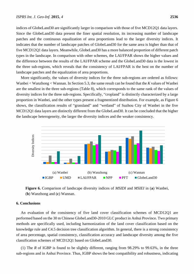
ISPRS Int. J. Geo-Inf. 2015, 4 2536
indices of GlobeLand30 are significantly larger in comparison with those of five MCD12Q1 data layers.
Since the GlobeLand30 data present the finer spatial resolution, its increasing number of landscape
patches and the continuous equalization of area proportions lead to the larger diversity indices. It
indicates that the number of landscape patches of GlobeLand30 for the same area is higher than that of
five MCD12Q1 data layers. Meanwhile, GlobeLand30 has a more balanced proportion of different patch
types in the landscape. In comparison with other schemes, the LAI/FPAR shows the higher values and
the difference between the results of the LAI/FPAR scheme and the GlobeLand30 data is the lowest in
the three sub-regions, which reveals that the consistency of LAI/FPAR is the best on the number of
landscape patches and the equalization of area proportions.
More significantly, the values of diversity indices for the three sub-regions are ordered as follows:
Wanbei < Wanzhong < Wannan. In Section 5.3, the same result can be found that the K values of Wanbei
are the smallest in the three sub-regions (Table 8), which corresponds to the same rank of the values of
diversity indices for the three sub-regions. Specifically, “cropland” is distinctly characterized by a large
proportion in Wanbei, and the other types present a fragmentized distribution. For example, as Figure 6
shows, the classification results of “grassland” and “wetland” of Suzhou City of Wanbei in the five
MCD12Q1 data layers are distinctly different from the GlobeLand30. It can be concluded that the higher
the landscape heterogeneity, the larger the diversity indices and the weaker consistency.
Figure 6. Comparison of landscape diversity indices of MSIDI and MSIEI in (a) Wanbei,
(b) Wanzhong and (c) Wannan.
6. Conclusions
An evaluation of the consistency of five land cover classification schemes of MCD12Q1 are
performed based on the 30 m Chinese GlobeLand30-2010 GLC product in Anhui Province. Two primary
methods are specifically used, including harmonization of the land cover classification based on the
knowledge rule and C4.5 decision tree classification algorithm. In general, there is a strong consistency
of area percentage, spatial consistency, classification accuracy and landscape diversity among the five
classification schemes of MCD12Q1 based on GlobeLand30.
(1) The R of IGBP is found to be slightly different, ranging from 98.29% to 99.63%, in the three
sub-regions and in Anhui Province. Thus, IGBP shows the best compatibility and robustness, indicating
Div
ersi
ty I
nd
ices
(a) Wanbei (b) Wanzhong (c) Wannan
IGBP UMD LAI/FPAR NPP PFT GlobeLand30

ISPRS Int. J. Geo-Inf. 2015, 4 2537
that the consistency of IGBP is the best on a regional scale. The PD of IGBP and UMD are the smallest
on each type in the three sub-regions, indicating that both IGBP and UMD present the best consistency.
(2) The O of LAI/FPAR has the lowest value, 58.17%, and its spatial consistency of “woodland” is
weak. Conversely, NPP has the best spatial consistency of “woodland” among the five schemes with an
O of 86.70%. Specially, the misclassification between “others” and “woodland” is the main cause
leading to the worst consistency of LAI/FPAR; that is, the “woodland” type of GlobeLand30 is largely
misclassified into the “barren land of LAI/FPAR.
(3) The 𝑝𝐴𝑖 and 𝑝𝑢𝑖 of “artificial surfaces” of LAI/FPAR scheme are the lowest in the three
sub-regions in comparison to the four other schemes of MCD12Q1 (Table 8). Furthermore, the OA of
NPP varies greatly in the three sub-regions, indicating that the consistency of NPP is the worst among
the five schemes.
(4) Since the landscape diversity indices of Wanbei, Wanzhong and Wannan are different from each
other, it shows the obvious spatial heterogeneity of the three sub-regions. The consistency of LAI/FPAR
is found to be the best on the landscape diversity in the three sub-regions. Meanwhile, the more
heterogeneous the landscape is, the weaker the consistency of the five land cover classification results
of MCD12Q1 become.
Given the great significance to evaluate and validate the quality and consistency of different GLC
products, this study evaluates the consistency of 500 m MCD12Q1 based on 30 m GlobeLand30 on a
provincial scale. This study can provide a methodological reference for evaluating the consistency of
different GLC products derived from multi-source and multi-resolution remote sensing datasets on
various spatial scales.
Acknowledgments
This work was financially supported by Anhui Provincial Natural Science Foundation
(Grant No. 1408085QF126), the Open Research Fund of Key Laboratory of Digital Earth Science,
Institute of Remote Sensing and Digital Earth, Chinese Academy of Sciences (No. 2014LDE012), the
211 Project of Anhui University (Grant No. KJQN1121) and the Leadership Introduction Project of
Academy and Technology of Anhui University (Grant No. 10117700024).
Author Contributions
Dong Liang accomplished this manuscript by designing the experiment, completing literature review,
preparing the validation dataset, making the related figures and tables, and finishing the whole
manuscript. Yan Zuo finished the data processing and analyzed the results. Meanwhile, this manuscript
is prepared and written under the guidance of Jinling Zhao. Other authors participated in the
implementation of this study by providing some helpful advice.
Conflicts of Interest
The authors declare no conflict of interest.

ISPRS Int. J. Geo-Inf. 2015, 4 2538
References
1. Pervez, M.S.; Henebry, G.M. Assessing the impacts of climate and land use and land cover change
on the freshwater availability in the Brahmaputra River basin. J. Hydrol. Region. Stud. 2015, 3,
285–311.
2. Clerici, N.; Paracchini, M.L.; Maes, J. Land-cover change dynamics and insights into ecosystem
services in European stream riparian zones. Ecohydrol. Hydrobiol. 2014, 14, 107–120.
3. Maitre, D.C.L.; Kotzee, I.M.; O’Farrell, P.J. Impacts of land-cover change on the water flow
regulation ecosystem service: Invasive alien plants, fire and their policy implications. Land Use
Policy 2014, 36, 171–181.
4. Pomara, L.Y.; Ledee, O.E.; Martin, K.J.; Zuckerberg, B. Demographic consequences of climate
change and land cover help explain a history of extirpations and range contraction in a declining
snake species. Glob. Chang. Biol. 2014, 20, 2087–2099.
5. Nagy, R.C.; Lockaby, B.G.; Zipperer, W.C.; Marzen, L.J. A comparison of carbon and nitrogen
stocks among land uses/covers in coastal Florida. Urban Ecosys. 2014, 17, 255–276.
6. Herold, M.; Woodcock, C.E.; Gregorio, A.D.; Mayaux, P.; Belward, A.S.; Latham, J.; Schmullius, C.C.
A joint initiative for harmonization and validation of land cover datasets. IEEE T. Geosci. Remote
Sens. 2006, 44, 1719–1727.
7. See, L.M.; Fritz, S. A method to compare and improve land cover datasets: application to the GLC-
2000 and MODIS land cover products. IEEE Trans. Geosci. Remote Sens. 2006, 44, 1740–1746.
8. Herold, M.; Mayaux, P.; Woodcock, C.E.; Baccini, A.; Schmullius, C. Some challenges in global
land cover mapping: An assessment of agreement and accuracy in existing 1 km datasets. Remote
Sens. Environ. 2008, 112, 2538–2556.
9. Tchuenté, A.T.K.; Roujean, J.L.; De Jong, S.M. Comparison and relative quality assessment of the
GLC2000, GLOBCOVER, MODIS and ECOCLIMAP land cover data sets at the African
continental scale. Int. J. Appl. Earth Obs. 2011, 13, 207–219.
10. Pérez-Hoyos, A.; García-Haro, F.J.; San-Miguel-Ayanz, J. Conventional and fuzzy comparisons of
large scale land cover products: application to CORINE, GLC2000, MODIS and GlobCover in
Europe. ISPRS J. Photogramm. Remote Sens. 2012, 74, 185–201.
11. Pérez-Hoyos, A.; García-Haro, F.J.; Valcarcel, N. Incorporating sub-dominant classes in the
accuracy assessment of large-area land cover products: application to GlobCover, MODISLC,
GLC2000 and CORINE in Spain. IEEE J. Sel. Top. Appl. Earth Obs. 2014, 1, 187–205.
12. Congalton, R.G.; Gu, J.; Yadav, K.; Ozdogan, M. Global land cover mapping: A review and
uncertainty analysis. Remote Sens. 2014, 6, 12070–12093.
13. Mora, B.; Tsendbazar, N.E.; Herold, M.; Arino, O. Global land cover mapping: Current status and
future trends. In Land Use & Land Cover Mapping in Europe; Manakos, I., Braun, M., Eds.;
Springer: Dordrecht, The Netherlands, 2014; pp. 11–30.
14. Loveland, T.R.; Belward, A.S. The IGBP-DIS global 1 km land cover data set, DISCover: First
results. Int. J. Remote Sens. 1997, 18, 3289–3295.
15. Reed, B.; Hansen, M.C. A comparison of the IGBP DISCover and University of Maryland 1 km
global land cover products. Int. J. Remote Sens. 2000, 21, 1365–1373.

ISPRS Int. J. Geo-Inf. 2015, 4 2539
16. Janssen, S.; Dumont, G.; Fierens, F.; Mensink C. Spatial interpolation of air pollution measurements
using CORINE land cover data. Atmos. Environ. 2008, 42, 4884–4903.
17. Feranec, J.; Hazeu, G.; Christensen, S.; Jaffrain, G. Corine land cover change detection in Europe
(case studies of the Netherlands and Slovakia). Land Use Policy 2007, 24, 234–247.
18. Friedl, M.A.; Sulla-Menashe, D.; Tan, B.; Schneider, A.; Ramankutty, N.; Sibley, A.; Huang, X.M.
MODIS Collection 5 global land cover: Algorithm refinements and characterization of new
datasets. Remote Sens. Environ. 2010, 114, 168–182.
19. Bartholomé, A.S.; Belward, E. GLC2000: a new approach to global land cover mapping from Earth
observation data. Int. J. Remote Sens. 2007, 26, 1959–1977.
20. Arino, O.; Gross, D.; Ranera, F.; Bourg, L.; Leroy, M.; Bicheron, P.; Latham, J.; Di Gregorio, A.;
Brockman, C.; Witt, R.; et al. GlobCover: ESA service for global land cover from MERIS. In
Proceedings of IEEE International Geoscience and Remote Sensing Symposium, Barcelona, Spain,
23–27 July 2007; pp. 2412–2415.
21. Li, M.; Mao, L.J.; Zhou, C.G.; Vogelmann, J.E.; Zhu, Z.L. Comparing forest fragmentation and its
drivers in China and the USA with Globcover v2.2. J. Environ. Manage. 2010, 91, 2572–2580.
22. Champeaux, J.L.; Masson, V.; Chauvin, F. ECOCLIMAP: A global database of land surface
parameters at 1 km resolution. Meteorol. Appl. 2005, 12, 29–32.
23. Chen, J.; Ban, Y.F.; Li, S.N. China: Open access to Earth land-cover map. Nature 2014, 514, 434.
24. Dong, J.; Xiao, X.; Sheldon, S.; Biradar, C.; Duong, N.D.; Hazarika, M. A comparison of forest
cover maps in Mainland Southeast Asia from multiple sources: PALSAR, MERIS, MODIS and
FRA. Remote Sens. Environ. 2012, 127, 60–73.
25. Dou, X.F.; Jiapa, A.; Li, Y.H.; Guan, Z.Z.; Wang, X.M.; Lv, Y.N.; Tian, L.L.; Li, X.; Zhang, X.C.;
Sun, Y.L.; et al. Remote sensing of land coverage and investigation of plague risk among small
mammals in Beijing, China. Chin. J. Vector Biol. Control. 2013, 24, 43–46. (In Chinese)
26. Li, Y.; Andrés, V.; Yang, W.; Chen, X.D.; Zhang, J.D.; Ouyang, Z.Y. Effects of conservation
policies on forest cover change in giant panda habitat regions, China. Land Use Policy 2013, 33,
42–53.
27. Yan, X.U.; Zhang, J. Detecting major phenological stages of rice using MODIS-EVI data and
Symlet11 wavelet in Northeast China. Acta Ecologica Sinica 2012, 7, 1–4. (In Chinese)
28. Moreno-Madriñán, M.J.; Rickman, D.L.; Ogashawara, I.; Irwin, D.; Ye, J.; Al-Hamdan, M.Z. Using
remote sensing to monitor the influence of river discharge on watershed outlets and adjacent coral
Reefs: Magdalena River and Rosario Islands, Colombia. Int. J. Appl. Earth Obs. 2015, 38, 204–215.
29. Zhao, X.; Xu, P.; Zhou, T.; Li, Q.; Wu, D.H. Distribution and variation of forests in China from
2001 to 2011: a study based on remotely sensed data. Forests 2013, 4, 632–649.
30. Weiss, M.; Baret, F.; Garrigues, S.; Lacaze, R. LAI and fAPAR CYCLOPES global products
derived from VEGETATION. Part 2: Validation and comparison with MODIS collection 4
products. Remote Sens. Environ. 2007, 110, 317–331.
31. Gross, D.; Dubois, G.; Pekel, J.F.; Mayaux, P.; Holmgren, M.; Prins, H.H.T.; Rondinini, C.; Boitani, L.
Monitoring land cover changes in African protected areas in the 21st century. Ecol. Inform. 2013,
14, 31–37.

ISPRS Int. J. Geo-Inf. 2015, 4 2540
32. Loveland, T.R.; Reed, B.C.; Brown, J.F.; Ohlen, D.O.; Zhu, Z.L.; Yang, L.M. Development of a
global land cover characteristics database and IGBP DISCover from 1 km AVHRR data. Int. J.
Remote Sen. 2000, 21, 1303–1330.
33. Hansen, M.C.; DeFries, R.S.; Townshend, J.R.G.; Sohlberg, R. Global land cover classification at
1 km spatial resolution using a classification tree approach. Int. J. Remote Sen. 2000, 21, 1331–1364.
34. Lotsch, A.; Tian, Y.; Friedl, M.A.; Myneni, R.B. Land cover mapping in support of LAI and FPAR
retrievals from EOS-MODIS and MISR: classification methods and sensitivities to errors. Int. J.
Remote Sen. 2003, 24, 1997–2016.
35. Myneni, R.B.; Hoffman, S.; Knyazikhin, Y.; Privette, J.; Glassy, J.; Tian, Y.; Wang, Y.; Song, X.;
Zhang, Y.; Smith G. Global products of vegetation leaf area and fraction absorbed PAR from year
one of MODIS data. Remote Sens. Environ. 2002, 83, 214–231.
36. Zhao, M.; Running, S.; Heinsch, F.A.; Nemani, R. MODIS-derived terrestrial primary production.
In Land Remote Sensing and Global Environmental Change; Ramachandran, B., Justice, C.O.,
Abrams, M.J., Eds.; Springer: Dordrecht, The Netherlands, 2011; pp. 635–660.
37. Chen, J.; Zhang, H.; Liu, Z.; Che, M.; Chen, B. Evaluating parameter adjustment in the MODIS
gross Primary production algorithm based on eddy covariance tower measurements. Remote Sens.
2014, 6, 3321–3348.
38. Chen, J.; Chen, J.; Liao, A.; Cao, X.; Chen, L.; Chen, X.; He, C.; Han, G.; Peng, S.; Lu, M.; et al.
Global land cover mapping at 30m resolution: A POK-based operational approach. ISPRS J.
Photogramm. Remote Sens. 2015, 103, 7–27.
39. Brovelli, M.; Molinari, M.; Hussein, E.; Chen, J.; Li, R. The first comprehensive accuracy
assessment of GlobeLand30 at a national level: methodology and results. Remote Sens. 2015, 7,
4191–4212.
40. Manakos, I.; Chatzopoulos-Vouzoglanis, K.; Petrou, Z.I.; Filchev, L.; Apostolakis, A.
Globalland30 mapping capacity of land surface water in Thessaly, Greece. Land 2015, 4, 1–18.
41. Hou, Y.; Wang, S.; Nan, Z.A. Rule-based land cover classification method for the Heihe River
Basin. Acta Geographica Sinica 2011, 66, 549–561. (In Chinese)
42. Ren, Z.C.; Zhu, H.Z.; Liu, X.N. Spatio-temporal differentiation of land covers on annual scale and
its response to climate and topography in arid and semi-arid region. Trans. Chin. Soc. Agric. Engin.
2012, 28, 205–214. (In Chinese)
43. Raynal, C.; Baux, D.; Theze, C.; Bareil, C.; Taulan, M.; Roux, A.F.; Claustres, M.; Tuffery-Giraud, S.;
des Georges, M. A classification model relative to splicing for variants of unknown clinical significance:
application to the CFTR gene. Hum. Mutat. 2013, 34, 774–784.
44. Saqib, F.; Dutta, A.; Plusquellic, J. Pipelined decision tree classification accelerator implementation
in FPGA (DT-CAIF). IEEE Trans. Comput. 2015, 64, 280–285.
45. Rucci, P.; Mandreoli, M.; Gibertoni, D.; Zuccalà, A.; Mariapia, F.; Lenzi, J.; Santoro, A. A clinical
stratification tool for chronic kidney disease progression rate based on classification tree analysis.
Nephrol. Dial. Transpl. 2014, 29, 603–610.
46. Durán-Alarcón, C.; Gevaert, C.M.; Mattar, C.; Jiménez-Muñoz, J.C.; Pasapera-Gonzalesc, J.J.;
Sobrino, J.A.; Silvia-Vidal, Y.; Fashé-Raymundo, O.; Chavez-Espiritu, T.W.; Santillan-Portilla N.
Recent trends on glacier area retreat over the group of Nevados Caullaraju-Pastoruri (Cordillera
Blanca, Peru) using Landsat imagery. J. S. Am. Earth Sci. 2015, 59, 19–26.

ISPRS Int. J. Geo-Inf. 2015, 4 2541
47. Gharehgozli, A.H.; Yu, Y.; Koster, R.D.; Udding, J.T. A decision-tree stacking heuristic minimising
the expected number of reshuffles at a container terminal. Int. J. Prod. Res. 2014, 52, 2592–2611.
48. Ahmad, A. Decision tree ensembles based on kernel features. Appl. Intell. 2014, 41, 855–869.
49. Salzberg, S.L. Book review: C4.5: Programs for machine learning by J. Ross Quinlan. Morgan
Kaufmann Publishers, Inc., 1993. Mach. Learn. 1994, 16, 235–240.
50. Joseph, L.R.; Nicewander, W.A. Thirteen ways to look at the correlation coefficient. Am. Stat. 1988,
42, 59–66.
51. He, Y.Q.; Bo, Y.C. A consistency analysis Of MODIS MCD12Q1 and MERIS Globcover land
cover datasets over China. In Proceedings of the 19th International Conference on Geoinformatics,
Shanghai, China, 24–26 June 2011; pp. 1–6.
52. Song, H.; Zhang, X.; Wang, Y.; Wang, M. Comparison of relative uniformity between GLOBCOVER
and MODIS land cover data sets. Trans. Chin. Soc. Agric. Engin. 2012, 15, 118–124. (In Chinese)
53. Stehman, S.V. Selecting and interpreting measures of thematic classification accuracy. Remote
Sens. Environ. 1997, 62, 77–89.
54. Thompson, W.D.; Walter, S.D. A reappraisal of the kappa coefficient. J. Clin. Epidemiol. 1988, 41,
949–958.
55. Romme, W.H.; Knight, D.H. Landscape diversity: The concept applied to Yellowstone Park.
Bioscience 1982, 32, 664–670.
56. Anhui Provincial Bureau of Statistics. Available online: http://www.ahtjj.gov.cn/tjj/
web/tjnj_view.jsp (accessed on 15 July 2015). (In Chinese)
57. Anhui Provincial Forestry Department. Available online: http://www.ahly.gov.cn/ (accessed on 15
July 2015). (In Chinese)
58. Xia, W.T.; Wang, Y.; Feng, Q.S.; Liang, T.G. Accuracy assessment of MODIS land cover product
of Gannan Prefecture. Pratacultural Sci. 2010, 27, 11–18. (In Chinese)
59. Yang, Y.; Liu, Y.B.; Ruan, R.Z.; Ye, C.; Lu, P.P. Scale-induced uncertainty in MODIS-based land
cover classification. J. Remote Sens. 2012, 16, 868–880. (In Chinese)
© 2015 by the authors; licensee MDPI, Basel, Switzerland. This article is an open access article
distributed under the terms and conditions of the Creative Commons Attribution license
(http://creativecommons.org/licenses/by/4.0/).