Biogeosciences, 11, 269–280, 2014www.biogeosciences.net/11/269/2014/doi:10.5194/bg-11-269-2014© Author(s) 2014. CC Attribution 3.0 License.

Biogeosciences

Open A

ccess

On the consistency of MODIS chlorophylla products in thenorthern South China Sea

S. L. Shang1,2, Q. Dong2, C. M. Hu3, G. Lin1, Y. H. Li 1, and S. P. Shang1,2

1Key Laboratory of Underwater Acoustic Communication and Marine Information Technology (Xiamen University),Ministry of Education of China, Xiamen 361005, China2Research and Development Center for Ocean Observation Technologies, Xiamen University, Xiamen 361005, China3College of Marine Science, University of South Florida, 140 Seventh Ave. S., St. Petersburg, FL 33701, USA

Correspondence to:S. L. Shang (slshang@xmu.edu.cn)

Received: 10 April 2013 – Published in Biogeosciences Discuss.: 2 May 2013Revised: 10 November 2013 – Accepted: 4 December 2013 – Published: 22 January 2014

Abstract. Chlorophyll a (Chl) concentrations derived fromsatellite measurements have been used in oceanographic re-search, for example to interpret eco-responses to environ-mental changes on global and regional scales. However, itis unclear how existing Chl products compare with eachother in terms of accuracy and consistency in revealing tem-poral and spatial patterns, especially in the optically com-plex marginal seas. In this study, we examined three MODIS(Moderate Resolution Imaging Spectroradiometer) Chl dataproducts that have been made available to the communityby the US National Aeronautics and Space Administra-tion (NASA) using community-accepted algorithms and de-fault parameterization. These included the products derivedfrom the OC3M (ocean chlorophyll three-band algorithmfor MODIS), GSM (Garver–Siegel–Maritorena model) andGIOP (generalized inherent optical properties) algorithms.We compared their temporal variations and spatial distri-butions in the northern South China Sea. We found thatthe three products appeared to capture general features suchas unique winter peaks at the Southeast Asian Time-seriesStudy station (SEATS, 18◦ N, 116◦ E) and the Pearl Riverplume associated blooms in summer. Their absolute magni-tudes, however, may be questionable in the coastal zones.Additional error statistics using field measured Chl as thetruth demonstrated that the three MODIS Chl products maycontain high degree of uncertainties in the study region. Rootmean square error (RMSE) of the products from OC3M andGSM (on a log scale) was about 0.4 and average percent-age error (ε) was∼ 115 % (Chl between 0.05–10.41 mg m−3,n = 114). GIOP with default parameterization led to higher

errors (ε = 329 %). An attempt to tune the algorithms basedon a local coastal-water bio-optical data set led to reducederrors for Chl retrievals, indicating the importance of localtuning of globally-optimized algorithms. Overall, this studypoints to the need of continuous improvements for algorithmdevelopment and parameterization for the coastal zones ofthe study region, where quantitative interpretation of the cur-rent Chl products requires extra caution.

1 Introduction

Chl a is the primary phytoplankton pigment for photo-synthesis, whose concentration (hereafter abbreviated asChl, mg m−3) has been commonly used as a phytoplank-ton biomass index by oceanographers. Over the past threedecades, an unprecedented view of the spatiotemporal pat-tern of Chl in the global ocean has been enabled by oceancolor satellites such as CZCS (Coastal Zone Color Scan-ner), SeaWiFS (Sea-Viewing Wide Field-of-View Sensor)and MODIS (Moderate Resolution Imaging Spectroradiome-ter) (McClain, 2009). Based on these observations, a bet-ter understanding of the ecosystem health and carbon cy-cling associated with environmental changes at both globaland regional scales has been achieved (e.g., Behrenfeld andBoss, 2006). Although the retrieval of Chl from satellite mea-surements is often problematic in optically complex coastalwaters due to interference from non-pigment color matters,i.e., colored dissolved organic matter (CDOM) and detri-tus (e.g., Carder et al., 1989), and the use of optical indices

Published by Copernicus Publications on behalf of the European Geosciences Union.

270 S. L. Shang et al.: On the consistency of MODIS chlorophylla products

for phytoplankton pigmentation has become increasingly ac-cepted (e.g., Cullen, 1982; Marra et al., 2007; Lee et al.,2011; Hirawake et al., 2011; Shang et al., 2011), Chl remainsa basic, routinely sampled, and widely accepted oceano-graphic parameter for oceanographers.

Among the past and present ocean color sensors, MODISis the major operational one at present and has been widelyused by researchers to study global and regional oceanogra-phy. Previous evaluation of MODIS Chl demonstrated thatMODIS Chl had moderately good agreement with measuredChl in oceanic waters (e.g., Zhang et al., 2006; Moore etal., 2009), while overestimation was often observed in tur-bid coastal waters (e.g., Darecki and Stramski, 2004; Mag-nuson et al., 2004; Werdell et al., 2009). Currently, there arethree standard (operational) MODIS Chl data products pro-vided by the US National Aeronautics and Space Administra-tion (NASA) Ocean Biology Processing Group (OBPG,http://oceancolor.gsfc.nasa.gov), which are derived from MODISremote sensing reflectance (Rrs, sr−1) after atmosphere cor-rection of MODIS measurements (http://oceancolor.gsfc.nasa.gov) over the ocean. The algorithms used to derive theseproducts are the OC3M (ocean chlorophyll three-band algo-rithm for MODIS) blue/green band ratio algorithm (O’Reillyet al., 2000), the GSM (Garver–Siegel–Maritorena model)semi-analytical inversion algorithm (Maritorena et al., 2002),and the GIOP generalized IOPs (inherent optical properties)algorithm (Franz and Werdell, 2010; Werdell et al., 2013).Fundamentally, the OC3M empirical algorithm is differentfrom the other two spectral optimization algorithms in twoaspects (also see pp. 3–4 in the IOCCG report (2006) on therationales of the various algorithms): (1) unlike the GSM andGIOP algorithms, the OC3M is not designed to differentiateChl from other in-water constituents (Fig. 1). This is because,similar to Chl, both CDOM and detrital particles absorb bluelight strongly, and the OC3M blue/green ratio algorithm can-not distinguish them explicitly. The GSM and GIOP are in-herently similar in design. They are both based on a quan-titative description of absorption and scattering propertiesof all optical components in the water, and the same semi-analytical reflectance model (Gordon, 1988) to describe howthese properties (i.e., IOPs) determine the water’s reflectancespectrum (i.e., spectralRrs). Chl is then derived simulta-neously with IOPs because Chl is a monotonous functionof phytoplankton pigment absorption coefficient (aph). BothGSM and GIOP use mathematical optimization approachesto search for an optimal solution. The difference lies solely inthe assumptions and parameterizations when modeling IOPs.For example, GSM uses fixed constants for the chlorophyll-specific phytoplankton pigment absorption coefficients (a∗

ph)

while the default GIOP usesa∗

ph as a function of Chl (Bricaudet al., 1995). Their performance can therefore be influencedby the model parameterization (IOCCG, 2006; Huang et al.,2013). (2) The algorithm inputs (MODIS-derivedRrs) arealso different. The inputs to the OC3M areRrs at 443, 488,

31

635

636

Fig. 1. Conceptual diagram of the OC3M (Route 1), and the GSM and GIOP 637

(Route 2). 638

639

RadianceSpectrum

Empirical Regression

Radiative Transfer Theory IOPs

Chl

1

2

Fig. 1. Conceptual diagram of the OC3M (route 1), and the GSMand GIOP (route 2).

and 547 nm, while the inputs to the GSM and GIOP areRrsdata from all six MODIS bands. MODISRrs data in the bluebands (412 and 443 nm) are usually of low quality owing tothe difficulties in atmospheric correction (e.g., Siegel et al.,2005; Bailey and Werdell, 2006), representing another im-portant uncertainty source for all three algorithms.

It has been well recognized that each algorithm has itsown strengths and weaknesses (e.g., O’Reilly et al., 1998;Werdell, 2009). However, while an increasing number ofusers from the oceanographic community are using the var-ious Chl products to interpret biogeochemical processes ortemporal changes, the consistency between these Chl prod-ucts is generally unknown, especially for marginal seas. Cancertain spatiotemporal patterns be revealed by one Chl prod-uct but masked by another?

In this study, we attempted to address this question by us-ing an extensive data set collected from a marginal sea. Wechose the South China Sea (SCS) as the study region, notonly because of the extensive effort in the past decade to col-lect field data but also because of its regional and global im-portance (e.g., Liu et al., 2002; Lin et al., 2003; Tang et al.,2004; Isoguchi et al., 2005; Tseng et al., 2005; Gan et al.,2009; Lin et al., 2010; Hong et al., 2011; Palacz et al., 2011;Xiu and Chai, 2011). Indeed, the SCS is the second largestmarginal sea in the world. Data analysis will in particularbe focused on the northern SCS (NSCS), where in situ datawere collected for algorithm tuning and product evaluation(Fig. 2).

The study focused on three easily accessible standard (op-erational) MODIS Chl products (hereafter abbreviated asC_OC3M, C_GSM, and C_GIOP). Our goal is to demon-strate the consistency or discrepancy among the biogeochem-ical features in the SCS derived from these three easily acces-sible Chl products, to diagnose potential reasons of productinconsistency or high uncertainty, and to seek for potentialsolutions to reduce the product uncertainties. Specifically,the analysis was through (1) comparison of Chl spatiotem-poral variations at the Southeast Asian Time-series Studystation (SEATS), two typical coastal upwelling zones, andthe Pearl River estuary; (2) evaluation of MODIS-derivedRrsand MODIS Chl products using field measuredRrs and Chlas the truth; and (3) regional tuning of the algorithms for theNSCS coastal zones based on a local bio-optics data set (Rrs,Chl, andaph).

Biogeosciences, 11, 269–280, 2014 www.biogeosciences.net/11/269/2014/

S. L. Shang et al.: On the consistency of MODIS chlorophylla products 271

32

640

641

642

Fig. 2. Map of the study region. QDU and YDU refer to upwelling zones off 643

Qiongdong and Yuedong (boundaries of the zones were defined following Jing et 644

al. (2011)). PRE refers to the Pearl River estuary, and SEATS refers to the 645

Southeast Asian Time- series Study station (18ºN, 116ºE). Blue circles show the 646

locations where concurrent MODIS Rrs data and in situ observed Chl were used 647

for algorithm evaluations. Red crosses show the locations where concurrent field 648

measured Rrs and Chl were used for algorithm evaluations，121 groups of which 649

were collected in the coastal waters (from the green dotted line towards the shore) 650

and were also used for further regional algorithm tuning. 651

652

653

SEATS

South China Sea

Taiw

an S

trait

105o E 109o E 113o E 117o E 121o E

16o N

20o N

24o N

28o N

China

Luzon

Luzon Strait

Tai

wan

YDU

QDU

PRE

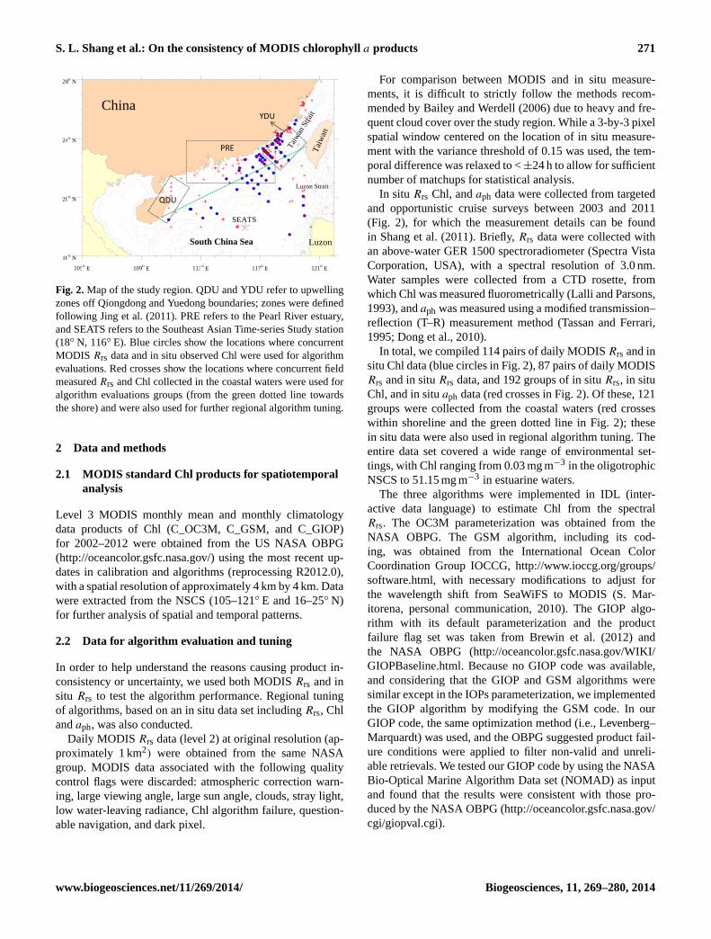
Fig. 2. Map of the study region. QDU and YDU refer to upwellingzones off Qiongdong and Yuedong boundaries; zones were definedfollowing Jing et al. (2011). PRE refers to the Pearl River estuary,and SEATS refers to the Southeast Asian Time-series Study station(18◦ N, 116◦ E). Blue circles show the locations where concurrentMODIS Rrs data and in situ observed Chl were used for algorithmevaluations. Red crosses show the locations where concurrent fieldmeasuredRrs and Chl collected in the coastal waters were used foralgorithm evaluations groups (from the green dotted line towardsthe shore) and were also used for further regional algorithm tuning.

2 Data and methods

2.1 MODIS standard Chl products for spatiotemporalanalysis

Level 3 MODIS monthly mean and monthly climatologydata products of Chl (C_OC3M, C_GSM, and C_GIOP)for 2002–2012 were obtained from the US NASA OBPG(http://oceancolor.gsfc.nasa.gov/) using the most recent up-dates in calibration and algorithms (reprocessing R2012.0),with a spatial resolution of approximately 4 km by 4 km. Datawere extracted from the NSCS (105–121◦ E and 16–25◦ N)for further analysis of spatial and temporal patterns.

2.2 Data for algorithm evaluation and tuning

In order to help understand the reasons causing product in-consistency or uncertainty, we used both MODISRrs and insitu Rrs to test the algorithm performance. Regional tuningof algorithms, based on an in situ data set includingRrs, Chlandaph, was also conducted.

Daily MODIS Rrs data (level 2) at original resolution (ap-proximately 1 km2) were obtained from the same NASAgroup. MODIS data associated with the following qualitycontrol flags were discarded: atmospheric correction warn-ing, large viewing angle, large sun angle, clouds, stray light,low water-leaving radiance, Chl algorithm failure, question-able navigation, and dark pixel.

For comparison between MODIS and in situ measure-ments, it is difficult to strictly follow the methods recom-mended by Bailey and Werdell (2006) due to heavy and fre-quent cloud cover over the study region. While a 3-by-3 pixelspatial window centered on the location of in situ measure-ment with the variance threshold of 0.15 was used, the tem-poral difference was relaxed to <±24 h to allow for sufficientnumber of matchups for statistical analysis.

In situ Rrs Chl, andaph data were collected from targetedand opportunistic cruise surveys between 2003 and 2011(Fig. 2), for which the measurement details can be foundin Shang et al. (2011). Briefly,Rrs data were collected withan above-water GER 1500 spectroradiometer (Spectra VistaCorporation, USA), with a spectral resolution of 3.0 nm.Water samples were collected from a CTD rosette, fromwhich Chl was measured fluorometrically (Lalli and Parsons,1993), andaph was measured using a modified transmission–reflection (T–R) measurement method (Tassan and Ferrari,1995; Dong et al., 2010).

In total, we compiled 114 pairs of daily MODISRrs and insitu Chl data (blue circles in Fig. 2), 87 pairs of daily MODISRrs and in situRrs data, and 192 groups of in situRrs, in situChl, and in situaph data (red crosses in Fig. 2). Of these, 121groups were collected from the coastal waters (red crosseswithin shoreline and the green dotted line in Fig. 2); thesein situ data were also used in regional algorithm tuning. Theentire data set covered a wide range of environmental set-tings, with Chl ranging from 0.03 mg m−3 in the oligotrophicNSCS to 51.15 mg m−3 in estuarine waters.

The three algorithms were implemented in IDL (inter-active data language) to estimate Chl from the spectralRrs. The OC3M parameterization was obtained from theNASA OBPG. The GSM algorithm, including its cod-ing, was obtained from the International Ocean ColorCoordination Group IOCCG,http://www.ioccg.org/groups/software.html, with necessary modifications to adjust forthe wavelength shift from SeaWiFS to MODIS (S. Mar-itorena, personal communication, 2010). The GIOP algo-rithm with its default parameterization and the productfailure flag set was taken from Brewin et al. (2012) andthe NASA OBPG (http://oceancolor.gsfc.nasa.gov/WIKI/GIOPBaseline.html. Because no GIOP code was available,and considering that the GIOP and GSM algorithms weresimilar except in the IOPs parameterization, we implementedthe GIOP algorithm by modifying the GSM code. In ourGIOP code, the same optimization method (i.e., Levenberg–Marquardt) was used, and the OBPG suggested product fail-ure conditions were applied to filter non-valid and unreli-able retrievals. We tested our GIOP code by using the NASABio-Optical Marine Algorithm Data set (NOMAD) as inputand found that the results were consistent with those pro-duced by the NASA OBPG (http://oceancolor.gsfc.nasa.gov/cgi/giopval.cgi).

www.biogeosciences.net/11/269/2014/ Biogeosciences, 11, 269–280, 2014

272 S. L. Shang et al.: On the consistency of MODIS chlorophylla products

2.3 Error statistics

To assess the similarity or difference between measuredand algorithm-derived parameters, four statistical indicatorswere calculated, following community-accepted standards(IOCCG, 2006; Moore et al., 2009). These indicators in-cluded the coefficient of determination (R2), mean absolutepercentage error (ε), bias (δ), and root mean square error(RMSE) in log scale, defined as follows:

ε =1

n

n∑i=1

|yi − xi |

xi

× 100% (1)

δ =1

n

n∑i=1

[log10(yi) − log10(xi)] (2)

RMSE=

√√√√1

n

n∑i=1

[log10(yi) − log10(xi)]2 (3)

wherex represents the measured parameter andy representsthe algorithm-derived parameter.

3 Results

Figure 3 shows MODIS Chl distributions in four months dur-ing spring, summer, fall, and winter. In general, all threeChl products showed similar seasonality and spatial distri-butions: (1) Chl is lower in spring and fall than in summerand winter; (2) Chl is lower in the offshore SCS (< 0.1 –∼ 0.1 mg m−3) than in nearshore waters (∼ 1 – > 1 mg m−3);and (3) there is a large patch of elevated Chl in and to thewest of the Luzon Strait in winter. However, some appar-ent differences among the three products were also found, asshown in Figs. 3 and 4. The seasonality in C-GIOP was notas apparent as in C_OC3M or C_GSM. While C_OC3M andC_GSM showed maxima in winter, C-GIOP showed ratherflat temporal changes between summer and winter. Field ob-servations showed high Chl during winter throughout theSCS basin (e.g., Chen, 2005; Ning et al., 2004), confirm-ing the observed patterns in C_OC3M and C_GSM. In addi-tion, within the Chl minimum season (i.e., spring), monthlyvariations for C_OC3M were quite different from those forC_GSM and C_GIOP. C_OC3M decreased consistently fromMarch to May while the fluctuations of C_GSM and C_GIOPwithin this time frame were not distinct. Unfortunately no insitu data, either published or unpublished, could be found tohelp clarify which monthly variation patterns during springwere more convincing.

While Figs. 3 and 4 showed general patterns of the threeChl products, their consistency and discrepancy are detailedat several targeted locations, as shown below.

33

654

Fig. 3. Climatological monthly mean Chl in the northern South China Sea in 655

March, July, October and December from three algorithms: (top) C_OC3M; 656

(middle) C_GSM; (bottom) C_GIOP. 657

658

Mar Jul Oct Dec

Fig. 3. Climatological monthly mean Chl in the northern SouthChina Sea in March, July, October and December from three al-gorithms: (top) C_OC3M; (middle) C_GSM; (bottom) C_GIOP.

4

24

25

Fig. 4. Monthly climatology of MODIS Chl for the northern South China Sea 26

(16-25ºN, 105-121ºE, the region of Fig. 3). 27

28

29

30

Month

Jan Feb Mar Apr May Jun Jul Aug Sep Oct Nov Dec

Ch

l (m

g/m

3)

0.0

0.5

1.0GSM

GIOP

OC3M

Ch

l(m

g m

-3)

Fig. 4. Monthly climatology of MODIS Chl for the northern SouthChina Sea (16–25◦ N, 105–121◦ E, the region depicted in Fig. 3).

3.1 SEATS

The SEATS (18◦ N, 116◦ E), located in the deep (> 3000 m)oligotrophic basin, was used to represent the SCS offshorewaters. All products showed similar seasonality of Chl, i.e.,elevated Chl in winter (Fig. 5a). This is consistent with insitu observations (Tseng et al., 2005). Very minor differ-ences emerged in the detailed month-to-month and inter-annual variations (Fig. 5b). This is also illustrated by thestrong correlation between C_GSM, C_GIOP and C_OC3M(R > 0.8, Fig. 6). When compared with the limited in situ data(red dots in Fig. 5b), differences were observed only for onedata point in winter 2010 when both C_GSM and C_GIOPshowed large departure from the in situ measurements. Notethat this difference could be natural because one data pointmay not be representative of the mean state of the month. Ingeneral, all three Chl products showed consistent temporalpatterns from this offshore SCS station.

Biogeosciences, 11, 269–280, 2014 www.biogeosciences.net/11/269/2014/

S. L. Shang et al.: On the consistency of MODIS chlorophylla products 273

5

31

Fig. 5. Monthly climatology (a) and monthly variations (b) of MODIS Chl at 32

SEATS. Red symbols refer to field measured Chl. 33

Month

Jan Feb Mar Apr May Jun Jul Aug Sep Oct Nov Dec

0.00

0.05

0.10

0.15

0.20

0.25

0.30

OC3M

GSM

GIOP

Ch

l (m

g m

-3)

2002 2003 2004 2005 2006 2007 2008 2009 2010 2011 2012

0.0

0.1

0.2

0.3

0.40.0

0.1

0.2

0.3

0.40.0

0.1

0.2

0.3

0.4OC3M

GSM

GIOP

(a)

(b)

Ch

l (m

g m

-3)

Year

Fig. 5. Monthly climatology (a) and monthly variations(b) ofMODIS Chl at SEATS. Red symbols refer to field measured Chl.

3.2 Summer upwelling zones

The NSCS is featured by upwelling (e.g., Xie et al., 2003;Gan et al., 2009; Hong et al., 2009; Jing et al., 2011). Theconsistency of the three Chl products was examined in twowell-known coastal upwelling zones in summer, which arethe upwelling zones off Qiongdong (QDU) and Yuedong(YDU) (see Fig. 2 for the locations).

Although the general patterns agreed with each other, thethree products showed some differences in the mean monthlyChl extracted from the two zones (Fig. 7). C_OC3M andC_GSM appeared to have stronger seasonality (i.e., largerdifference between annual maximum and annual minimum)than C_GIOP. More importantly, winter highs were more dis-tinct than summer highs based on C_OC3M and C_GSM.This appeared contradictory from the seasonal patterns ob-served from very limited in situ measurements (e.g., Zhanget al., 1997), and from the knowledge that these two zoneswere short of nutrient supplies during winter (dry season)but were rich in nutrients owing to upwelling and land-basedrunoff during summer (wet season). This is possibly becauseChl is overestimated in winter for C_OC3M and C_GSM.For C_OC3M, interference from non-phytoplankton mat-ters (CDOM and detritus), which are commonly rich inthese coastal waters, would cause Chl overestimation. ForC_GSM, the globally optimized parameterization (Mari-torena et al., 2002), such as Chl-specific absorption coef-ficient, may not be applicable in these coastal waters. Thisdid not occur to C_GIOP possibly because data alongshore

6

34

35

Fig. 6. Scatter plots showing the correlation between (a) C_OC3M and C_GSM; 36

(b) C_OC3M and C_GIOP at SEATS. 37

38

C_OC3M (mg m-3

)

0.0 0.1 0.2 0.3 0.4

C_

GS

M (

mg m

-3)

0.0

0.1

0.2

0.3

0.4

C_OC3M (mg m-3

)

0.0 0.1 0.2 0.3 0.4

C_

GIO

P (

mg m

-3)

0.0

0.1

0.2

0.3

0.4(a) (b)

y=0.776*x+0.019

R=0.88, N=97

y=0.792*x-0.010

R=0.82, N=97

Fig. 6. Scatter plots showing the correlation between(a) C_OC3Mand C_GSM;(b) C_OC3M and C_GIOP at SEATS.

0.0

1.0

2.0

3.0

4.0

5.0

Month

01/2002 01/2003 01/2004 01/2005 01/2006 01/2007 01/2008 01/2009 01/2010 01/2011 01/2012 01/2013

Chl (mg m

-3)

0.0

1.0

2.0

3.0

4.0

5.0

(a)

(b)

GSMOC3M

GIOPOC3M*

Fig. 7. Monthly variations of MODIS Chl in the Qiongdong (a) and Yuedong (b) upwelling zones;

arrows indicate summer.Fig. 7.Monthly variations of MODIS Chl in the Qiongdong(a) andYuedong(b) upwelling zones; arrows indicate summer.

were filtered during data processing. Unfortunately, on theGIOP website there is no information on how the alongshoredata are screened. One possibility is that those data fall underthe preset product failure conditions (http://oceancolor.gsfc.nasa.gov/WIKI/GIOPBaseline.html).

3.3 Pearl River plume

There are two big rivers in the SCS, the Pearl River and theMekong River. They contribute large amounts of fresh wateras well as nutrients and other matters to the nearby ocean,thus having significant impact on the biogeochemistry of theSCS. Here we chose the Pearl River plume as an exampleto examine the time series derived from the three Chl dataproducts.

Figure 8a shows the monthly climatology of C_OC3M,C_GSM and C_GIOP in the vicinity of the Pearl River es-tuary (PRE, 21–2◦ N, 112–118◦ E) in four months of differ-ent seasons. All three products consistently showed a distinctriver plume extending eastward in summer.

To further compare the Chl products in nearshore waters,monthly climatology in January and July were extracted fromwaters shallower than 50 m. The monthly climatologies forthe C_OC3M and C_GIOP were higher in July than in Jan-uary (e.g., 3.30 mg m−3 versus 2.22 mg m−3). This is con-sistent with the known seasonal patterns, i.e., higher Chl

www.biogeosciences.net/11/269/2014/ Biogeosciences, 11, 269–280, 2014

274 S. L. Shang et al.: On the consistency of MODIS chlorophylla products

38

   

   

   

          

677

Fig. 8. (a) Monthly climatology of MODIS Chl in the vicinity of the Pearl River 678

estuary in January, April, July and October. The isobath of 50 m is annotated on 679

the January image of C_OC3M; (b) MODIS Chl anomaly (in percentage) in 680

January and July of 2002-2012 for the nearshore waters of the Pearl River 681

estuary (depth < 50m). 682

683

-350

-300

-250

-200

-150

-100

-50

0

50

100

150

200

Per

cent

age

anom

aly

(%)

OC3MGSMGIOP

-40

-30

-20

-10

0

10

20

30

40

50

Per

cent

age

anom

aly

(%)

2002 2003 2004 2005 2006 2007 2008 2009 2010 2011 2012Year

Jan

Jul

Jan Apr Jul Oct OC3M

GIOP

GSM

OC3M*

(a)

(b)

Fig. 8. (a)Monthly climatology of MODIS Chl in the vicinity of thePearl River estuary in January, April, July and October. The isobathof 50 m is annotated on the January image of C_OC3M;(b) MODISChl anomaly (in percentage) in January and July of 2002–2012 forthe nearshore waters of the Pearl River estuary (depth < 50 m).

in summer (wet season) than in winter (dry season) (e.g.,Zhang, 2001). However, C_GSM was almost the same in Jan-uary and July (3.42 mg m−3 versus 3.36 mg m−3). This couldbe due to the improper parameterization of the GSM model,or due to high uncertainties in the MODISRrs data in theblue bands in nearshore waters.

The differences between the Chl products are further illus-trated in the monthly anomaly patterns (Fig. 8b). Note thatthe monthly anomalies were calculated by simply deducingthe monthly climatology from the monthly mean. In January,C_OC3M showed a strong positive anomaly in 2007, andC_GSM and C_GIOP appeared to have anomalies in the op-posite directions. In July, the anomaly patterns of the threeproducts were relatively similar to each other. A strong neg-ative anomaly was found in 2004 in all three products, whilethe years of positive anomalies showed some discrepancy.Assuming that+25 % higher than climatology indicated apositive anomaly, a unique positive anomaly was found in2009 for C_OC3M and C_GSM, while a > 25 % anomalywas found in 2008 for C_GIOP. Based on these observations,it could be inferred that summer blooms associated with riverplumes and upwelling (e.g., Gan et al., 2010; Dai et al., 2008)

were relatively weak in 2004. The bloom would however beinferred to be strong in 2009 if it was based on C_OC3Mand C_GSM, or in 2008 if it was based on C_GIOP. Thus,without field-based validations (e.g., measured Chl, river dis-charges, nutrient fluxes, wind forcing, etc.), interpretation ofthe standard satellite-based Chl data products requires extracaution for nearshore waters of the NSCS. Algorithm tuningbased on local data is thus advocated for these waters.

4 Discussion

4.1 Causes of the inconsistency

The above results showed consistent Chl patterns in theNSCS basin waters but large differences in upwelling zonesand river plumes from the three products. In order to help di-agnose the reasons of such similarity and discrepancy, in situdata were used to evaluate algorithm performance.

First, MODIS-derivedRrs data were used as the algorithminputs to derive Chl, and then compared with the measuredChl. Figure 9 shows the evaluation results and the statisticsare listed in Table 1. The average percentage errors all ex-ceeded the desired level of accuracy for satellite-derived Chl(35 %, Bailey and Werdell, 2006) in this dynamic marginalsea. Most of the MODIS-derived Chl values were overesti-mated, as indicated by the positiveδ. However, except forC_GIOP, MODIS-derived Chl agreed with in situ Chl rea-sonably well (ε ∼ 113 % to 118 %, RMSE∼ 0.380 to 0.400,δ 0.069 to 0.145, see Table 1). The poorer performance ofC_GIOP is due in part to its poor performance in shallowwaters (< 50 m, see red dots in Fig. 9c;ε = 441 %,δ = 0.464,see Table 1).

To test whether the discrepancy resulted from the algo-rithms or from uncertainties in the MODISRrs, the accuracyof MODIS Rrs was evaluated using in situRrs (Fig. 10). Ingeneral, MODISRrs agreed well with ground truth data ex-cept at 412 nm. This is consistent from other reported results(e.g., Siegel et al., 2005; Bailey and Werdell, 2006; Antoineet al., 2008; Dong, 2010).R2 ranged between 0.72 and 0.86andε was < 26 % for bands 443, 488, 531 and 547 nm, whileε were 31 % and 49 % for 412 nm and 667 nm. Because the443, 488, and 547 nm bands were used to estimate Chl inthe OC3M algorithm, the relatively lower uncertainties inthe MODISRrs in these bands suggest that C_OC3M wouldbe influenced less by the MODISRrs uncertainties than theother two products, which used all six bands to estimate Chl.

The uncertainties introduced by the algorithms were fur-ther examined by using in situRrs as the algorithm input,with the derived Chl compared with the measured Chl. Re-sults are shown in Table 1 and Fig. 11. When comparedwith the field measured Chl, Chl derived from in situRrsagreed better than Chl derived from MODISRrs because ofthe reduction in theRrs uncertainties and because of the re-moval of the mismatch between satellite pixel size and in

Biogeosciences, 11, 269–280, 2014 www.biogeosciences.net/11/269/2014/

S. L. Shang et al.: On the consistency of MODIS chlorophylla products 275

Table 1.Error statistics between derived and in situ Chl.

Algorithm R2 ε (%) RMSE δ N n

MODIS Rrs derived (in situ Chl = 0.05–10.41 mg m−3,mean = 0.87, std = 1.36)

OC3M 0.39 118 0.380 0.145 114 114OC3M∗ 0.40 63 0.290 0.015 114 114GSM 0.35 113 0.400 0.069 114 112GSM∗ 0.29 76 0.329 0.029 114 112GIOP 0.23 329 0.600 0.340 114 111GIOP∗ 0.32 111 0.396 0.081 114 110

MODIS Rrs derived (< 50 m) (Chl = 0.09–10.41 mg m−3,mean = 1.27, std = 1.70)

OC3M 0.32 155 0.433 0.225 64 64OC3M∗ 0.32 75 0.330 0.012 64 64GSM 0.28 147 0.438 0.163 64 63GSM∗ 0.24 80 0.356 −0.002 64 63GIOP 0.16 441 0.692 0.464 64 61GIOP∗ 0.26 131 0.431 0.108 64 63

In situRrs derived (Chl = 0.03–51.15 mg m−3,mean = 2.89,std = 6.63)

OC3M 0.81 111 0.363 0.132 192 192GSM 0.85 94 0.342 0.086 192 174GIOP 0.13 256 0.548 0.163 192 160

∗ N is the number ofRrs data input, whilen is the number of valid retrievals.

situ sample size. Both OC3M and GSM performed well (R2

∼ 0.81–0.85) although the error indices still exceeded themission specifications (35 %). Similar to the above satellite-based analysis, GIOP showed lowerR2 (0.13) and higher er-ror indices than the other two algorithms (e.g.,ε ∼ 256 %).The results suggest that the uncertainties in the three Chlproducts were mostly attributed to the inversion algorithmsas opposed to imperfect atmospheric correction. However,it is unclear what caused the relatively poor performance ofthe GIOP algorithm in this marginal sea. Indeed, in an algo-rithm round-robin comparison, all 17 algorithms includingGIOP were found to perform reasonably well in estimatingChl (Brewin et al., 2014). We speculate that the algorithm pa-rameterization of GIOP requires a major tuning for the studyregion.

Thus, differences in the MODIS Chl data products ap-peared to have resulted mainly from the algorithm designin addressing the dependence of reflectance on the variousin-water constituents. In the offshore (bottom depth >200 m)SCS whereaph / at at 443 nm of the surface ocean rangesfrom 0.2 to 0.8 (at refers to the total absorption coefficientwithout water,n = 119; Shang, unpublished data), water’soptical properties are predominantly driven by phytoplank-ton, or the optical properties of phytoplankton, CDOM, anddetritus co-vary. Therefore, the three Chl products showedalmost the same spatial and temporal patterns although their

9

50

Fig. 9. Comparison between MODIS Rrs derived Chl and field measured Chl 51

where MODIS Chl was derived using three algorithms and their tuned forms: (a) 52

OC3M; (b) GSM; (c) GIOP; (d) tuned OC3M (OC3M*); (e) tuned GSM (GSM*); 53

(f) tuned GIOP (GIOP*). Red symbols refer to data collected from nearshore 54

waters (depth <50 m). Statistics of the algorithm performance are listed in Table 55

1. 56

57

Measured Chl (mg m-3

)

0.01 0.1 1 10 100

Der

ived

Ch

l (m

g m

-3)

0.01

0.1

1

10

100

0.01 0.1 1 10 100

0.01

0.1

1

10

100

0.01 0.1 1 10 100

0.01

0.1

1

10

100

(a) OC3M (b) GSM (c) GIOP

0.01 0.1 1 10 100

0.01

0.1

1

10

100

0.01 0.1 1 10 100

0.01

0.1

1

10

100

0.01 0.1 1 10 100

0.01

0.1

1

10

100

(d) OC3M* (e) GSM* (f) GIOP*

Fig. 9.Comparison between MODISRrs derived Chl and field mea-sured Chl where MODIS Chl was derived using three algorithmsand their tuned forms:(a) OC3M; (b) GSM; (c) GIOP; (d) tunedOC3M (OC3M*); (e) tuned GSM (GSM*); and(f) tuned GIOP(GIOP*). Red symbols refer to data collected from nearshore waters(depth < 50 m). Statistics of the algorithm performance are listed inTable 1.

magnitudes varied slightly. In coastal upwelling zones andriver plumes where the water is optically complex with sig-nificant amount of CDOM and detrital particles (both organicand mineral particles) (adg / at at 443 nm could be up to 0.97,whereadg refers to the absorption coefficients of the sum ofCDOM and detritus, Shang, unpublished data; also see Honget al., 2005; Du et al., 2010), larger differences were foundfrom the three Chl products. The OC3M empirical algorithmwas not designed to differentiate Chl from other in-waterconstituents. The spectral optimization algorithms such asGSM and GIOP were designed to separate Chl from otherin-water constituents, yet their performance was influencedby their fixed parameterization (IOCCG, 2006; Huang et al.,2013). For example, the parameterization for backscatteringcoefficients of particles (including both organic and mineralparticles) may not reflect the truth in coastal waters rich inmineral particles. Failure in finding an optimal solution maybe one reason for the pixel speckling in the C_GSM imagesand those masked nearshore pixels in the C_GIOP images(Fig. 8a). These failed pixels would cause a bias in calculat-ing the mean and anomalies. Clearly, when time series datawere analyzed, image series would need to be examined inorder to identify these potential artifacts and to improve datainterpretation.

4.2 Algorithm tuning

Based on the above analysis, in coastal waters the threeChl products are not consistent and might not reflect thetruth. In order to solve the problem, we tuned the algorithmsfor coastal waters of the NSCS. In situ data for algorithmtuning were specifically collected from waters between the

www.biogeosciences.net/11/269/2014/ Biogeosciences, 11, 269–280, 2014

276 S. L. Shang et al.: On the consistency of MODIS chlorophylla products

40

693

Fig. 10. Comparison between MODIS-derived Rrs and field measured Rrs. 694

695

0.000 0.003 0.006 0.009 0.012 0.0150.000

0.003

0.006

0.009

0.012

0.015

0.000 0.003 0.006 0.009 0.012 0.0150.000

0.003

0.006

0.009

0.012

0.015

0.000 0.005 0.010 0.015 0.020 0.025

MO

DIS

Rrs

(sr-1

)

0.000

0.005

0.010

0.015

0.020

0.025

In situ Rrs (sr-1)

0.000 0.005 0.010 0.015 0.020 0.0250.000

0.005

0.010

0.015

0.020

0.025

0.000 0.005 0.010 0.015 0.020 0.0250.000

0.005

0.010

0.015

0.020

0.025

0.000 0.002 0.004 0.006 0.008 0.010 0.012 0.0140.000

0.002

0.004

0.006

0.008

0.010

0.012

0.014

(a) 412 nm

(f) 667 nm

(c) 488 nm

(e) 547 nm

(b) 443 nm

(d) 531 nm

= 31%RMSE = 0.145

R2 = 0.70 (n = 87)

= 26%RMSE = 0.121

R2 = 0.72 (n = 87)

= 18%RMSE = 0.090

R2 = 0.78 (n = 87)

= 20%RMSE = 0.102

R2 = 0.86 (n = 87)

= 20%RMSE = 0.107

R2 = 0.86 (n = 87)

= 49%RMSE = 0.220

R2 = 0.93 (n = 85)

Fig. 10.Comparison between MODIS-derivedRrs and field measuredRrs.

11

61

62

Fig. 11. Comparison between field measured Chl and in situ Rrs derived Chl 63

using three algorithms: (a) OC3M; (b) GSM; (c) GIOP. Statistics of algorithm 64

performance are listed in Table 1. 65

66

0.01 0.1 1 10 100

Deriv

ed

Ch

l (m

g m

-3)

0.01

0.1

1

10

100

0.01 0.1 1 10 100

0.01

0.1

1

10

100

Measured Chl (mg m-3

)

0.01 0.1 1 10 100

0.01

0.1

1

10

100(a) (c)(b)

n=192

R2=0.81

RMSE=0.363

n=160

R2=0.13

RMSE=0.548

n=174

R2=0.85

RMSE=0.342

Fig. 11.Comparison between field measured Chl and in situRrs derived Chl using three algorithms:(a) OC3M;(b) GSM;(c) GIOP. Statisticsof algorithm performance are listed in Table 1.

shoreline and the green dotted line in Fig. 2 (generally in theregions of PRE, QDU, and YDU). To facilitate data compar-ison, hereafter the regionally tuned algorithms are referred toas OC3M∗, GSM∗, and GIOP∗.

The C_OC3M was derived fromRrs ratios as

Chl = 10(c0+c1×Rratio+c2×R2ratio+c3×R3

ratio+c4×R4ratio) (4)

Rratio = log10

(Max(Rrs(443),Rrs(488))

Rrs(547)

)(5)

wherec0–c4 are the algorithm coefficients determined fromnonlinear regression between Chl andRrs ratios. An in situdata set ofRrs and Chl (n = 121, sampled from coastal wa-ters between the shoreline and the green dotted line in Fig. 2),

was used to determine the algorithm coefficients, with resultsshown in Fig. 12 (blue dots and blue curve). For comparison,also shown in the figure, are the original NOMAD data set(http://seabass.gsfc.nasa.gov/, green crosses) and the defaultOC3M algorithm (green curve). Note that the local data cov-ered almost the entire range of the NOMAD data set exceptfor extremely clear waters. MODIS Chl calculated using theregionally tuned OC3M∗ were then compared to in situ Chl(Fig. 9d), which showed substantial improvements. The er-rors were almost halved (ε decreased from 126 % to 63 %,and RMSE decreased from 0.380 to 0.290; see Table 1).

Biogeosciences, 11, 269–280, 2014 www.biogeosciences.net/11/269/2014/

S. L. Shang et al.: On the consistency of MODIS chlorophylla products 277

42

702

Fig. 12. Algorithm tuning for the OC3M band-ratio algorithm. All data were 703

collected from in situ measurements. The green crosses and green curve are for 704

the OC3M algorithm with default parameterization, while the blue dots 705

represent local data collected from NSCS coastal waters. The blue curve is the 706

locally tuned algorithm, with parameterization annotated on the figure. 707

log max(Rrs(443),Rrs(488))/Rrs(547)

-0.8 -0.6 -0.4 -0.2 0.0 0.2 0.4 0.6 0.8 1.0 1.2

log

Chl

-3.0

-2.0

-1.0

0.0

1.0

2.0

3.0

NOMADNSCSOC3MOC3M*

y=-0.0500-2.5043x+5.6447x2-6.2525x3+0.6421x4

(R2=0.84, N=121)

Fig. 12.Algorithm tuning for the OC3M band-ratio algorithm. Alldata were collected from in situ measurements. The green crossesand green curve are for the OC3M algorithm with default param-eterization, while the blue dots represent local data collected fromNSCS coastal waters. The blue curve is the locally tuned algorithm,with parameterization annotated on the figure.

In GSM and GIOP,aph, adg, andbbp (particle backscatter-ing coefficient) are modeled as

aph(λ) = Chl× a∗

ph(λ) (6)

adg(λ) = a(λ0) × exp(−Sadg(λ − λ0)) (7)

bbp(λ) = bbp(λ0) × (λ

λ0)−η (8)

where Chl,adg(λ0) andbbp(λ0) are three scalar variables tobe derived from a knownRrs spectrum via optimization.λ0is a reference wavelength and is generally set as 440 nm. Inthe models,a∗

ph, Sadg (spectral slope ofadg) andη (power co-efficient of bbp) can be tuned using local data. In the GSMparameterization,Sadg andη are optimized as 0.0206 nm−1

and 1.03373 for global waters, respectively; anda∗

ph is alsooptimized as a fixed spectrum for global waters, for example,aph(443) = Chl· 0.05582 (Maritorena et al., 2002). In the de-fault GIOP parameterization,Sadg= 0.018 nm−1, andη anda∗

ph are no longer fixed spectrum but using functional formsfollowing that of the QAA Eq. (9), Lee et al. (2002, 2009)and Bricaud et al. (1995) Eq. (10), respectively:

η = 2.2× (1− 1.2× e−0.9×

rrs(443)rrs(555) ), (9)

(rrs(λ) =Rrs(λ)

0.52+ 1.7× Rrs(λ))

a∗

ph(λ) = A(λ) × Chl−B(λ). (10)

Table 2.Coefficients ofa∗ph(λ) for tuned GSM and GIOP.

GSM: GIOP:a∗ph(λ)

Bands a∗ph(λ) =A(λ) Chl −B(λ)

A B

412 0.0672 0.067 0.299443 0.0754 0.071 0.281488 0.0498 0.046 0.299531 0.0176 0.019 0.292547 0.0125 0.014 0.308667 0.0264 0.027 0.209

The parameters ofa∗

ph, Sadg, and η were tuned, and aftertrial and error we found that the following combination ledto the lowest error budgets for Chl retrievals. (1) GSM∗:Sadg= 0.018 nm−1 andη were calculated from Eq. (9). Theywere in fact the default setting of the GIOP;a∗

ph was re-derived based on an in situaph and Chl data set collected inthe target region, for example, nowaph(443) = Chl· 0.0754(Table 2). (2) GIOP∗: There was no change forSadg andη

while a∗

ph derived from regression based on the same in situaph and Chl data set used for the GSM∗ (Table 2). In otherwords, for GIOP, only the coefficients ofa∗

ph were tuned,while the GSM was tuned more thoroughly, with all threefunctions changed.

The regionally tuned algorithms were then used to calcu-late Chl using the MODISRrs as the algorithm inputs, andcompared to concurrent in situ Chl. Evaluation results for theregionally tuned GSM∗ and GIOP∗ are shown in Fig. 9e andf and Table 1. Similar to OC3M∗, the algorithms showed no-table improvements over the original forms. For example,ε

was reduced from 113 % to 76 % for the GSM∗ and 329 %to 111 % for the GIOP∗. More substantial improvementswere found for shallow waters (< 50 m, Table 1), whereε

reduced from 441 % to 131 % for the GIOP∗. Such improve-ments are better than those obtained from similar efforts forthe Mediterranean Sea and western Canada coastal waters(D’Ortenzio et al., 2002; Komick et al., 2009). However, theerrors are still higher than those from the OC3M∗, suggest-ing more room for future algorithm development (Werdell etal., 2013).

Finally, based on the improved error statistics, OC3M∗

was chosen to re-derive the spatiotemporal patterns for thethree coastal zones (Figs. 7 and 8a). In the QDU and YDU,the absolute magnitudes of Chl decreased while the seasonalpatterns, i.e., peaking in winter, remained. Regardless of thetuning, it seems impossible to completely remove the inter-ference of CDOM and detritus to the blue light absorption.However, in the PRE, the serious overestimation of Chl fromthe OC3M was partially corrected using the OC3M∗.

www.biogeosciences.net/11/269/2014/ Biogeosciences, 11, 269–280, 2014

278 S. L. Shang et al.: On the consistency of MODIS chlorophylla products

5 Summary

Three MODIS Chl products are currently being used by theresearch community to address global and regional ques-tions. These are derived from the OC3M, GSM, and GIOPalgorithms. Yet their accuracy and consistency between eachother are often unclear for marginal seas. Using a field dataset collected from the NSCS, we evaluate the accuracy of thethree MODIS Chl data products as well as their consistencyin revealing spatial and temporal patterns under various sce-narios.

The temporal changes and spatial distribution patterns inthe three Chl data products differed mainly in optically com-plex nearshore waters, where certain spatiotemporal patternsrevealed by one Chl product can be masked by another. Inoffshore SCS waters where optical properties are mostlydominated by phytoplankton, Chl seasonality and interan-nual changes derived from the three products were similar.This was mainly attributed to the algorithm design as op-posed to the uncertainties in the inputRrs. The in situ valida-tion (using in situRrs as input) showed RMSE errors > 0.3 inlog scale and percentage errors > 90 % for all three Chl algo-rithms. While nearly identical statistical results were foundfor OC3M and GSM, GIOP showed significant deviationfrom the ground truth, possibly due to the incompatibility be-tween its default parameterization and the optical propertiesof the NSCS. The three algorithms were then locally tuned.Tuning of the OC3M resulted in significant improvement inproduct accuracy for coastal waters, while the improvementfrom the tuned GSM and GIOP algorithms was not as pro-found.

Overall, for the study region of the NSCS it is suggestedthat (1) all three standard MODIS products yielded reason-able spatial and temporal patterns for the offshore basin wa-ters; (2) current C_GIOP (with its default parameterization)is not proper for coastal water analysis because nearshoredata are masked; (3) a clear specification of Chl productin oceanographic time-series studies would facilitate cross-study comparisons; and (4) regional tuning of the algorithmsfor coastal waters of the NSCS is necessary to reduce productuncertainty.

Acknowledgements.This work was supported jointly by NSF-China (#40976068), the National Basic Research Program of China(#2009CB421201), the Ministry of Science and Technology ofChina (#2013BAB04B00), and the University of South Florida.We thank the crew of the R/VDongfanghong IIand Yanping II,and J. Wu, X. Ma, X. Sui, W. Zhou, W. Wang, M. Yang, C. Duand G. Wei for their help in collecting in situ data. We also thankthe NASA OBPG for providing MODIS data. We acknowledgethe help from three anonymous reviewers who provided extensivecomments and suggestions to improve this manuscript.

Edited by: K. Fennel

References

Antoine, D., d’Ortenzio, F., Hooker, S. B., Bécu, G., Gentili, B.,Tailliez, D., and Scott, A. J.: Assessment of uncertainty in theocean reflectance determined by three satellite ocean color sen-sors (MERIS, SeaWiFS and MODIS-A) at an offshore site in theMediterranean Sea (BOUSSOLE project), J. Geophys. Res., 113,C07013, doi:10.1029/2007JC004472, 2008.

Bailey, S. W. and Werdell, P. J.: A multi-sensor approach for the on-orbit validation of ocean color satellite data products, Remote.Sens. Environ., 102, 12–23, 2006.

Behrenfeld, M. J. and Boss, E.: Beam attenuation and chloro-phyll concentration as alternative optical indices of phytoplank-ton biomass, J. Mar. Res., 64, 431–451, 2006.

Brewin, R. J., Dall’Olmo, G., Sathyendranath, S., and Hardman-Mountford, N. J.: Particle backscattering as a function of chloro-phyll and phytoplankton size structure in the open-ocean, Opt.Express, 20, 17632–17652, 2012.

Brewin, R. J. W., Sathyendranath, S., Müller, D., Brockmann, C.,Deschamps, P.-Y., Devred, E., Doerffer, R., Fomferra, N., Franz,B., Grant, M., Groom, S., Horseman, A., Hu, C., Krasemann, H.,Lee, Z. P., Maritorena, S., Mélin, F., Peters, M., Platt, T., Regner,P., Smyth, T., Steinmetz, F., Swinton, J., Werdell, J., and WhiteIII, G. N.: The Ocean Colour Climate Change Initiative: III.A round-robin comparison on in-water bio-optical algorithms,Remote. Sens. Environ., in press, doi:10.1016/j.rse.2013.09.016,2014.

Bricaud, A., Babin, M., Morel, A., and Claustre, H.: Variability inthe chlorophyll-specific absorption coefficients of natural phyto-plankton: analysis and parameterization, J. Geophys. Res., 100,13321–13332, 1995.

Carder, K. L., Steward, R. G., Harvey, G. R., and Ortner, P. B.: Ma-rine humic and fulvic acids: their effects on remote sensing ofocean chlorophyll, Limnol. Oceanogr., 34, 68–81, 1989.

Chen, L.: Spatial and seasonal variations of nitrate-based new pro-duction and primary production in the South China Sea, DeepSea Res. Pt. 1, 52, 319–340, 2005.

Cullen, J. J.: The deep chlorophyll maximum: comparing verticalprofiles of chlorophyll a, Can. J. Fish. Aquat. Sci., 39, 791–803,1982.

D’Ortenzio, F., Marullo, S., Ragni, M., Ribera d’Alcalà, M., andSantoleri, R.: Validation of empirical SeaWiFS algorithms forchlorophyll-a retrieval in the Mediterranean Sea: A case studyfor oligotrophic seas, Remote. Sens. Environ., 82, 79–94, 2002.

Darecki, M. and Stramski, D.: An evaluation of MODIS and SeaW-iFS bio-optical algorithms in the Baltic Sea, Remote. Sens. Env-iron., 89, 326–350, 2004.

Dai, M., Zhai, W., Cai, W., Callahan, J., Huang, B., Shang, S.,Huang, T., Li, X., Lu, Z., Chen, W., and Chen, Z.: Effects of anestuarine plume-associated bloom on the carbonate system in thelower reaches of the Pearl River estuary and the coastal zone ofthe northern South China Sea, Cont. Shelf Res., 28, 1416–1423,doi:10.1016/j.csr.2007.04.018, 2008.

Dong, Q.: Derivation of phytoplankton absorption properties fromocean color and its application, Ph.D. thesis, Xiamen University,China, 2010.

Du, C., Shang, S., Dong, Q., Hu, C., and Wu, J.: Characteristics ofchromophoric dissolved organic matter in the nearshore watersof the western Taiwan Strait, Estuar. Coast. Shelf. S., 88, 350–356, doi:10.1016/j.ecss.2010.04.014, 2010.

Biogeosciences, 11, 269–280, 2014 www.biogeosciences.net/11/269/2014/

S. L. Shang et al.: On the consistency of MODIS chlorophylla products 279

Franz, B. A. and Werdell, P. J.: A generalized framework for mod-eling of inherent optical properties in ocean remote sensing ap-plications, Ocean Optics XX, Anchorage, Alaska, 27th Sept.–1stOct, 2010.

Gan, J. P., Li, L., Wang, D. X., and Guo, X. G.: Interac-tion of a river plume with coastal upwelling in the north-eastern South China Sea, Cont. Shelf Res., 29, 728–740,doi:10.1016/j.csr.2008.12.002, 2009.

Gan, J. P., Lu, Z. M., Dai, M. H., Cheung, A. Y. Y., Liu,H. B., and Harrison, P.: Biological response to intensifiedupwelling and to a river plume in the northeastern SouthChina Sea: A modeling study, J. Geophys. Res., 115, C09001,doi:10.1029/2009jc005569, 2010.

Gordon, H. R., Brown, O. B., Evans, R. H., Brown, J. W., Smith,R. C., Baker, K. S., and Clark, D. K.: A semianalytic radiancemodel of ocean color, J. Geophys. Res., 93, 10909–10924, 1988.

Hirawake, T., Takao, S., Horimoto, N., Ishimaru, T., Yamaguchi,Y., and Fukuchi, M.: A phytoplankton absorption-based primaryproductivity model for remote sensing in the Southern Ocean,Polar Biol., 34, 291–302, 2011.

Hong, H., Wu, J., Shang, S., and Hu, C.: Absorption and fluo-rescence of chromophoric dissolved organic matter in the PearlRiver Estuary, South China, Mar. Chem., 97, 78–89, 2005.

Hong, H., Zhang, C., Shang, S., Huang, B., Li, Y., Li, X., and Zhang,S.: Interannual variability of summer coastal upwelling in theTaiwan Strait, Cont. Shelf Res., 29, 479–484, 2009.

Hong, H., Liu, X., Chiang, K.-P., Huang, B., Zhang, C., Hu,J., and Li, Y.: The coupling of temporal and spatial varia-tions of chl a concentration and the East Asian monsoons inthe southern Taiwan Strait, Cont. Shelf Res., 31, S37–S47,doi:10.1016/j.csr.2011.02.004, 2011.

Huang, S. H., Li, Y. H., Shang, S. P., and Shang S. L.: Impact ofcomputational methods and spectral models on the retrieval ofoptical properties via spectral optimization, Opt. Express, 21:6257–6273, 2013.

IOCCG: Remote Sensing of Inherent Optical Properties: Funda-mentals, Tests of Algorithms, and Applications, in: Reportsof the International Ocean-Colour Coordinating Group, No. 5,edited by: Lee, Z. P., IOCCG, Dartmouth, Canada, 126, 2006.

Isoguchi, O., Kawamura, H., and Ku-Kassim, K.-Y.: El Niño–related offshore phytoplankton bloom events around the SpratleyIslands in the South China Sea, Geophys. Res. Lett., 32, L21603,doi:10.1029/2005GL024285, 2005.

Jing, Z., Qi, Y., and Du, Y.: Upwelling in the continental shelf ofnorthern South China Sea associated with 1997–1998 El Niño, J.Geophys. Res., 116, C02033, doi:10.1029/2010JC006598, 2011.

Komick, N., Costa, M., and Gower, J.: Bio-optical algorithm eval-uation for MODIS for western Canada coastal waters: An ex-ploratory approach using in situ reflectance, Remote. Sens. Env-iron., 113, 794–804, 2009.

Lalli, C. M. and Parsons, T. R.: Biological Oceanography: An In-troduction, Pergamon Press, Oxford, 1993.

Lee, Z. P., Carder, K. L., and Arnone, R. A.: Deriving inherent opti-cal properties from water color: a multiband quasi-analytical al-gorithm for optically deep waters, Appl. Optics, 41, 5755–5772,2002.

Lee, Z. P., Lubac, B., Werdell, J., and Arnone, R.: An Update ofthe Quasi-Analytical Algorithm (QAA_v5), International OceanColor Group Software Report, 2009.

Lee, Z. P., Du, K., Voss, K. J., Zibordi, G., Lubac, B., Arnone, R.,and Weidemann, A.: An inherent-optical-property-centered ap-proach to correct the angular effects in water-leaving radiance,Appl. Optics, 50, 3155–3167, 2011.

Lin, I. I., Lien, C. C., Wu, C. R., Wong, G. T., Huang, C. W., andChiang, T. L.: Enhanced primary production in the oligotrophicSouth China Sea by eddy injection in spring, Geophys. Res. Lett.,37, L16602, doi:10.1029/2010GL043872, 2010.

Lin, I., Liu, W. T., Wu, C.-C., Wong, G. T., Hu, C., Chen, Z., Liang,W.-D., Yang, Y., and Liu, K.-K.: New evidence for enhancedocean primary production triggered by tropical cyclone, Geo-phys. Res. Lett., 30, 1718, doi:10.1029/2003GL017141, 2003.

Liu, K. K., Chao, S. Y., Shaw, P. T., Gong, G. C., Chen, C. C., andTang, T.: Monsoon-forced chlorophyll distribution and primaryproduction in the South China Sea: observations and a numericalstudy, Deep Sea Res. Pt. 1, 49, 1387–1412, 2002.

Magnuson, A., Harding, L. W., Mallonee, M. E., and Adolf, J. E.:Bio-optical model for Chesapeake Bay and the Middle AtlanticBight, Estuar. Coast. Shelf. S., 61, 403–424, 2004.

Maritorena, S., Siegel, D. A., and Peterson, A. R.: Optimization ofa semianalytical ocean color model for global-scale applications,Appl. Optics, 41, 2705–2714, 2002.

Marra, J., Trees, C. C., and O’Reilly, J. E.: Phytoplankton pigmentabsorption: a strong predictor of primary productivity in the sur-face ocean, Deep-Sea Res. I, 54, 155–163, 2007.

McClain, C. R.: A decade of satellite ocean color observations∗,Annu Rev Mar Sci, 1, 19-42, 2009.

Moore, T. S., Campbell, J. W., and Dowell, M. D.: A class-basedapproach to characterizing and mapping the uncertainty of theMODIS ocean chlorophyll product, Remote. Sens. Environ., 113,2424–2430, 2009.

Ning, X., Chai, F., Xue, H., Cai, Y., Liu, C., and Shi, J.: Physical-biological oceanographic coupling influencing phytoplanktonand primary production in the South China Sea, J. Geophys. Res.,109, C10005, doi:10.1029/2004JC002365, 2004.

O’Reilly, J., Maritorena, S., Mitchell, B. G., Siegel, D., Carder, K.L., Garver, S., Kahru, M., and McClain, C.: Ocean color chloro-phyll algorithms for SeaWiFS, J. Geophys. Res., 103, 24937–24953, 1998.

O’Reilly, J. E., Maritorena, S., Siegel, D., and O’Brien, M. C.:Ocean color chlorophyll a algorithms for SeaWiFS, OC2, andOC4: version 4, in: SeaWiFS postlaunch technical report se-ries, volume 11, SeaWiFS postlaunch calibration and validationanalyses, part 3, edited by: Hooker, S. B. and Firestone, E. R.,Greenbelt, Maryland: NASA Goddard Space Flight Center, 9–23, 2000.

Palacz, A. P., Xue, H., Armbrecht, C., Zhang, C., and Chai,F.: Seasonal and inter-annual changes in the surface chloro-phyll of the South China Sea, J. Geophys. Res., 116, C09015,doi:10.1029/2011JC007064, 2011.

Shang, S., Dong, Q., Lee, Z., Li, Y., Xie, Y., and Behrenfeld,M.: MODIS observed phytoplankton dynamics in the TaiwanStrait: an absorption-based analysis, Biogeosciences, 8, 841–850, doi:10.5194/bg-8-841-2011, 2011.

Shang, S., Li, L., Li, J., Li, Y., Lin, G., and Sun, J.: Phytoplanktonbloom during the northeast monsoon in the Luzon Strait border-ing the Kuroshio, Remote. Sens. Environ., 124, 38–48, 2012.

Siegel, D. A., Maritorena, S., Nelson, N. B., and Behrenfeld, M. J.:Independence and interdependencies among global ocean color

www.biogeosciences.net/11/269/2014/ Biogeosciences, 11, 269–280, 2014

280 S. L. Shang et al.: On the consistency of MODIS chlorophylla products

properties: Reassessing the bio-optical assumption, J. Geophys.Res., 110, C07011, doi:10.1029/2004JC002527, 2005.

Tang, D. L., Kawamura, H., and Guan, L.: Long-time observationof annual variation of Taiwan Strait upwelling in summer sea-son, Monitoring of Changes Related to Natural and ManmadeHazards Using Space Technology, 33, 307–312, 2004.

Tassan, S. and Ferrari, G. M.: An alternative approach to absorp-tion measurements of aquatic particles retained on filters, Lim-nol. Oceanogr., 40, 1358–1368, 1995.

Tseng, C. M., Wong, G. T. F., Lin, I. I., Wu, C. R., and Liu, K. K.: Aunique seasonal pattern in phytoplankton biomass in low-latitudewaters in the South China Sea, Geophys. Res. Lett., 32, L08608,doi:10.1029/2004GL022111, 2005.

Werdell, P. J.: Global bio-optical algorithms for ocean colorsatellite applications, AGU EOS Transactions, 90, p. 4,doi:10.1029/2009EO010005, 2009.

Werdell, P. J., Franz, B. A., Bailey, S. W., Feldman, G. C., Boss,E., Brando, V. E., Dowell, M., Hirata, T., Lavender, S. J., andLee, Z.: Generalized ocean color inversion model for retrievingmarine inherent optical properties, Appl. Optics, 52, 2019–2037,2013.

Werdell, P. J., Bailey, S. W., Franz, B. A., Harding, Jr, L. W., Feld-man, G. C., and McClain, C. R.: Regional and seasonal variabil-ity of chl a in Chesapeake Bay as observed by SeaWiFS andMODIS-Aqua, Remote Sens Environ, 113, 1319–1330, 2009.

Xie, S. P., Xie, Q., Wang, D., and Liu, W. T.: Summer upwelling inthe South China Sea and its role in regional climate variations, J.Geophys. Res., 108, 3261, doi:10.1029/2003JC001867, 2003.

Xiu, P. and Chai, F.: Modeled biogeochemical responses tomesoscale eddies in the South China Sea, J. Geophys. Res., 116,C10006, doi:10.1029/2010JC006800, 2011.

Zhang, C. Y., Hu, C. M., Shang, S. L., Muller-Karger, F. E., Li, Y.,Dai, M. H., Huang, B. Q., Ning, X. R., and Hong, H. S.: Bridg-ing between SeaWiFS and MODIS for continuity of chlorophyll-a concentration assessments off Southeastern China, Remote.Sens. Environ., 102, 250–263, 2006.

Zhang, F., Yang, Y., and Huang, B.Q.: Impact of nutrients on thechlorophyll a concentration in the Taiwan Strait. In: Collectionof Oceanography Research (7), edited by: Hong, H. S., Beijing,Ocean Press, 81–88, 1997. (in Chinese with English abstract).

Zhang, F.: Seasonal variation features of chlorophyll a content inTaiwan Strait, Journal of Oceanography in Taiwan Strait, 20,314–318, 2001(in Chinese with English abstract).

Biogeosciences, 11, 269–280, 2014 www.biogeosciences.net/11/269/2014/