evaluation of the anisotropic analytical algorithm aaa … abstract the aim of this thesis is to...

Master of Science thesis in Radiation Physics

Evaluation of the Analytical Anisotropic Algorithm

(AAA) in lung tumours for 6 MV photon energy.

Erik Nilsson

Supervisors: Anna Bäck & Roumiana Chakarova

Department of Radiation Physics

Göteborg University

January 2009

1

Table of Contents

TABLE OF CONTENTS...................................................................................................................................... 1

ABSTRACT........................................................................................................................................................... 2

ABBREVIATIONS ............................................................................................................................................... 3

INTRODUCTION................................................................................................................................................. 3

MATERIALS AND METHODS.......................................................................................................................... 4

MONTE CARLO .................................................................................................................................................... 4

AAA ................................................................................................................................................................... 6

The configuration algorithm........................................................................................................................... 6

The dose calculation algorithm...................................................................................................................... 6

TEST GEOMETRIES ............................................................................................................................................... 7

EXPERIMENTAL MEASUREMENTS ........................................................................................................................ 9

SIMPLIFIED CLINICAL CASE................................................................................................................................ 11

RESULTS AND DISCUSSION ......................................................................................................................... 12

LUNG PHANTOM WITHOUT BONE ....................................................................................................................... 12

PHANTOM WITH BONE ....................................................................................................................................... 17

Phantom with bone profiles across the bone................................................................................................ 18

Phantom with bone profiles along the bone ................................................................................................. 21

CLINICAL CASES ................................................................................................................................................ 24

CONCLUSION.................................................................................................................................................... 26

ACKNOWLEDGMENTS .................................................................................................................................. 27

APPENDIX I ....................................................................................................................................................... 28

FIELD SIZE 10 X 10 CM2

..................................................................................................................................... 28

FIELD SIZE 4 X 4 CM2

......................................................................................................................................... 32

OUTPUT FACTORS ............................................................................................................................................. 35

APPENDIX II...................................................................................................................................................... 36

BEAMNRC STEP 1............................................................................................................................................. 36

BEAMNRC STEP 2............................................................................................................................................. 38

DOSXYZ............................................................................................................................................................ 41

Phantoms with and without bone ................................................................................................................. 41

Clinical Cases .............................................................................................................................................. 43

REFERENCES.................................................................................................................................................... 45

2

Abstract

The aim of this thesis is to evaluate how the Analytical Anisotropic Algorithm, AAA, calculates the

dose to lung tumours. Comparisons are made to film and TLD measurements as well as Monte Carlo

simulations. Two different cases are studied; a tumour centrally in the lung and a tumour close to a

bone. In addition to comparisons in lung phantoms two clinical cases are evaluated.

There’s a good agreement between Monte Carlo and experimental measurements. AAA is generally

in compliance with MC, but doesn’t account for all scattering effects in the interface between

different mediums. AAA also has a tendency to overestimate the dose to a denser medium after the

lung. Comparisons between the phantoms and the clinical cases are sometimes difficult because of

different geometries and varying densities within the same medium. Effects also seem to vary with

field size.

3

Abbreviations

AAA – Analytical Anisotropic Algorithm

CT – Computed Tomography

HU – Houndsfield Units

MC – Monte Carlo

MU – Monitor Units

OF – Output factor

SSD – Source to Surface Distance

TLD - Thermoluminescent Dosimeter

Introduction

In radiotherapy treatment planning systems are used to calculate dose distributions in the target

volume and organs at risk and their accuracy is therefore of great importance. Of significant

importance is also the speed of the calculations and as a consequence the dose planning algorithms

employ approximations. Known limitations of these algorithms are often seen in heterogeneous

medium1 due to the difficulties of accurately approximating electron transport at interface of

mediums with different densities and in regions where electron equilibrium does not exist. Different

algorithms have different limitations and before implementation of a new algorithm, an evaluation of

its limitations is necessary2.

The aim of this work is to evaluate how Varian’s Analytical Anisotropic Algorithm (AAA) calculates the

dose in lung tumours for 6 MV photon energy. Lung tumours were chosen since this geometry is a

challenge for the algorithm performance, i.e. the tumour is of higher density than the lung, the lung

itself is surrounded by higher density materials like muscles and bone. Another reason for choosing

lung tumours is AAA’s improved accuracy in low density mediums compared to its predecessor the

Pencil Beam Convolution algorithm3.

This is a continuation of a previous work4 where the AAA was evaluated for different phantom

geometries by experimental measurements and compared to the Eclipse pencil beam convolution

algorithm. Here Monte Carlo simulations are performed in addition to experimental measurements

which don’t limit the comparisons to phantoms, but also allows corresponding clinical cases to be

evaluated.

4

Materials and Methods

The thesis can be divided into three steps. The first step was to improve the flexibility of the existing

Monte Carlo model of the Varian 600C accelerator5 when producing phase spaces for different field

sizes. The following step was to perform measurements and calculations in phantom material. Two

different cases have been considered, namely a lung tumour centrally in the lung and a tumour close

to bone. This step was carried out using phantoms consisting of Solid Water (manufacturer RMI),

lung equivalent material (RMI) with electron density 0,292 relative to water and bone equivalent

material (RMI) with electron density 1,707 relative to water in the case with the bone. In the third

and last step corresponding cases were analysed by Monte Carlo and Eclipse AAA, but in a clinical

situation based on CT-images of real patients.

Monte Carlo

The Monte Carlo simulations were performed using the BEAMnrc, a general purpose modelling

system for radiotherapy units6. BEAMnrc is based on the EGSnrc code for electron and photon

transport and handles energies from the keV range to the TeV range.

A model3 of the Varian 600C treatment unit in room 3 at Sahlgrenska University Hospital was used,

but modified to perform the simulation in two steps. A phase space file, which is a file containing

information about the particles charge, direction, energy, position and statistical weight at a certain

plane, was created just below the secondary collimators, fig 1. To improve performance several,

variance reduction techniques were used for example directional bremsstrahlung splitting and

electron range rejection7. A full list of variance reduction techniques used and settings can be found

in Appendix II. The phase space file is then used as input data for producing a phase space below the

jaws thus eliminating the need to re-simulate the top of the treatment unit when the field size is

altered. A possible flaw of the two-step method is that back scattering of the jaws may be

unaccounted for, but this is generally considered negligible in practice.

5

Figure 1: Schematic representation of the treatment unit.

The secondary phase space is further used in DOSxyz to calculate dose distributions of interest.

DOSxyz is a program included in the BEAMnrc distribution and allows dose calculations in phantoms

created either from CT-images or defined voxel by voxel. The new two-step method of space file

generation was validated by experimental data from the treatment unit as well as by data from the

treatment planning system Eclipse and by results from the original Monte Carlo model using a water

phantom in DOSxyz. Several field sizes were validated through comparing OF (output factors) as well

as depth and cross profiles, for details see Appendix I. In order to get the absolute dose by Monte

Carlo simulations, the MC results were normalized to the value calculated at 10 cm depth, at the

isocenter for 10 cm by 10 cm field, i.e. the calibration geometry. The normalization factor 7,6336E-17

for this accelerator was found to correspond to 1 Gy. In DOSxyz the particles were recycled 10 times

and radially redistributed to improve statistics and the uncertainty in the dose after normalization

varies between 2-5% depending on the depth. The energy for when the particles were terminated

was for electrons, ECUT, 700 keV (521 keV for DOSXYZ) and for photons, PCUT, 0.010 MeV. A

detailed list of all parameters is included in the Appendix II. For each of the phantom cases two voxel

sizes were used, the first with a voxel size of 0.25 x 0.25 x 0.5 cm3 and the second with a voxel size of

First Phase Space

Secondary Phase Space

Jaws

Secondary Collimators

Primary Collimators

Target

Flattening Filter

Phantom

6

0.5 x 0.5 x 0.2 cm3. The first case with a better resolution in the x,y plane, which was used to create

the cross profiles. The second one with better resolution in depth was used to normalize the cross

profiles in isocenter to a more accurate depth dose. When the cross profiles were symmetrical in the

x,y direction, i.e. in the lung phantom without bone, the profile shown is the average of the two. The

profiles were created with the program statdose which is a part of the BEAMnrc package. The dose

given is the dose to the defined medium.

AAA

The Analytical Anisotropic Algorithm, AAA, is a 3D pencil beam convolution-superposition algorithm

and implemented in Varian’s treatment planning system Eclipse. The AAA dose calculation model

consists of two components, the configuration algorithm and the actual dose calculation algorithm8.

The configuration algorithm

The configuration algorithm is used to characterize the clinical beam for a specific treatment unit

based on type of particle, fluence and energy and store the data in a phase space. The phase space is

created by a multiple source model consisting of: A primary photon source, an extra focal photon

source and an electron contamination source.

The primary photon source models the bremsstrahlung resulting from the accelerated electrons’

interaction with the target using pre-calculated Monte Carlo methods. A mean energy radial curve

takes into account the effects of the flatting filter by describing how the mean energy decreases with

increased distance from the central axis. A radial intensity profile takes into account how the fluence

varies with the distance from the central axis.

The extra focal photon source models the secondary photons generated in the flattening filter and

the primary collimator. It’s positioned just below at the bottom plane of the flattening filter creating

a broader beam compared to the primary source. The source is modelled based of the primary

source and takes no consideration to the off-axis variation of the spectrum 9.

The electron contamination source models the electrons mainly created through Compton scattering

from the head of the treatment unit and air. It’s modelled with a depth-dependent curve describing

lateral electron contamination dose.

The dose calculation algorithm

The patient’s body volume is divided into voxels determined by the size of the chosen calculation

grid. The voxels are divergent and aligned with the beam fan line. For each voxel the mean electron

density is computed based on CT images. The beam is then divided into small beamlets where the

cross section of the beamlet matches the voxel. For each beamlet the dose is calculated based on the

three different sources and their properties.

7

The dose from the primary and secondary photons are calculated the same way, but based on data

from their respective sources. Monoenergetic energy deposition pencil beam kernels are constructed

using Monte Carlo methods. The monoenergetic kernels are superpositioned to form polyenergetic

pencil beam kernels based on the spectrum of the beamlet. Scatter kernels determine the scattering

in the mediums. The scattering is corrected by scaling by the average density not only in the direction

of the pencil beam but also in 16 lateral directions.

The dose from the contamination electrons are determined by a convolution between the fluence of

the electrons, the energy deposition function and a scatter kernel. Changes in the spectrum due to

source to phantom distance are not accounted for9.

In Eclipse a calculation grid of .25 cm by .25 cm by .25 cm was used. The server build was 7.5.49.3 SP2

and client build was 8.1.18.7379 SP2 using the 8.1.17 version of AAA.

Test geometries

To see how the AAA performed in heterogeneous media and in low density medium i.e. lung tissue a

lung phantom was created using a lung equivalent material and Solid Water(R). Creating a physical

phantom also offers the opportunity to further validate the Monte Carlo simulations for a situation

where no physical measurements can be made and Monte Carlo simulations becomes the sole

reference. The field was a symmetric 7x7 cm2 and the isocenter was in the middle of the tumour at a

depth of 5cm and thus the SSD was 95 cm. Measurements were made at four different levels in the

phantom, fig 2, at the top of the tumour, in the middle of the tumour which also is the isocenter, at

the bottom of the tumour and finally at the interface between lung and water at a depth of 8 cm.

Identical phantoms were created in Eclipse and in DOSxyz.

The next step was to introduce even larger differences in density thus adding a bone which in a

clinical situation could correspond to a rib. Apart from the bone the phantom, fig 3, is very similar to

the phantom above, but a bone equivalent material was of course used in addition to the one above.

The isocenter was a depth of 3 cm, the SSD was 97 cm and the field size 7x7 cm2. Measurements

were made at three different levels. Identical phantoms were again created in Eclipse and DOSxyz.

In Eclipse the Solid Water was set to 0 HU, the lung -708 HU and the bone 752 HU. In DOSxyz the

materials are defined by ICRU standards and the type of medium is chosen and then their densities

can be set to custom values. The corresponding mass densities for the different material were 1.84 g

cm-3

for the bone 0.3 g cm-3

for the lung and 1 g cm-3

for water.

8

Figure 2: Transversal and coronal views of the lung phantom through the isocenter. Positions where

measurements were conducted are marked I-IV. 5 cm of water was added to the sides closest to the tumour

in the coronal view to make sure all scattering effects were accounted for.

2 cm

2 cm

2 cm

2 cm

20 cm

Position I Position II Position III

Position IV

Lung phantom

Transversal view

Solid Water

Lung equivalent material

20 cm

3 cm

3.5 cm

16.5 cm

Coronal view

3.5 cm

5 cm

9

Figure 3: Transversal and coronal views of the bone phantom in the isocenter. For better reference the

projection of bone in the coronal view is shown in the isocenter plane. Positions where measurements were

conducted are marked I-III. . 5 cm of water was added to the sides closest to the tumour in the coronal view

to make sure all scattering effects were accounted for.

Experimental measurements

All measurements were made on the Varian 600C treatment unit in room 3 at Sahlgrenska University

Hospital operating at photon energy 6 MV. The treatment unit is calibrated so that 120 MU deliver

an absorbed dose of 1 Gy in water at the isocenter at 10 cm depth for 10x10 cm field. The dose

calibration was tested before and after each measurement to eliminate the effects of accelerator

instability. Temperature and pressure were taken into account and a farmer type ionization chamberi

and electrometerii was used to conduct the dose test.

The Gafchromiciii EBT film was used for relative measurements and Harshaw TLD-100 (LiF:Mg, Ti)

square chips 3.2 x 3.2 x 0.9 mm to determine absolute dose to which the cross profiles were

normalized to. A calibration intended to obtain absolute values for the film was made, but due to too

i TB3001-2030, PTW Freiburg , Freiburg, Germany

ii Elektra Precision Electrometer model A serial 105, Precitron AB, Uppsala, Sweden

iii Gafchromic EBT, International Speciality Products, Wayne NJ, USA

2 cm

2 cm

2 cm

2 cm

20 cm

Position II Position I

Position III

Bone phantom

Transversal view across the bone

Bone equivalent material

Lung equivalent material

3 cm

3.5 cm

16.5 cm

Coronal view

3.5 cm

5 cm

16.5 cm

Solid Water

10

high uncertainties of the calibration the method of normalizing the film to the dose of the TLD was

chosen.

For each position in the phantom three pieces of film were used from three different sheets and

from different parts of the sheets. Each piece of film was marked with its position in the phantom,

the sheet which it came from and its alignment in order for the film to be scanned in the same

direction. To keep track of the direction of the film is important due to the anisotropic properties of

the film. To scan the film using the same part of the scanner is also very important since the

sensitivity is anisotropic. After exposure to 250 MUs (scaled to 70 MUs in graphs) the films were

stored in a dark box for 24h before being scanned in an Epson 1680 scanner with the resolution 300

dpi and 48 bit colours using Adobe Photoshop CS2 to import the pictures. All pictures were stored in

.tif format with no compression. The pictures were then analysed in RITiv. An 11x11 median filter was

applied. Due to the way the pictures are imported into RIT and cropped it is not always obvious

where the field starts and some uncertainties in position are therefore present.

The TLD were annealed each time before usage and allowed to slowly cool off. They were individually

marked and calibrated with Co-60 in solid water and their individual sensitivities obtained with

uncertainty < 2%. Two of the most accurate were used as reference dosimeters. The sensitivity

factors were updated after three measurements.

The solid water cylinder representing the tumour in the phantom cases was identical to the one used

in the film measurements with the exception that small holes were made to embed the TLDs, fig 4.

The phantom was firmly held together with tape to avoid air pockets and any unwanted

displacement and exposed to 70 MU.

Figure 4: The Solid Water cylinder that represents the tumour in the phantoms. To the right is the one with

holes for the TLDs.

The reference TLDs were exposed to 70 MU in a 10 x 10 cm2 field at a depth of 10 cm in Solid

Water(R). The TLDs were analysed in a Toledo TLD readerv . Each reading was corrected by the

sensitivity factors and converted to absolute dose, equation 1.

jj

refref

ref

j SRSR

DD *

*= Equation 1.

iv RIT 113 v5.1, Radiology Imaging Technology inc., Colorado Spring, USA

v 654 Toledo TLD reader, Pitman, Weybridge, England

11

Where Dj is the absolute dose for the j-th TLD, Dref is the 70 MU dose received by the reference

dosimeter corrected by eventual daily deviation, Rj is the j-TLD reading, Sref and Sj are the

corresponding sensitivity factors.

Simplified clinical case

Two different patients matching the two different phantom cases and roughly matching existing

Monte Carlo simulated field sizes were chosen. Field sizes in Eclipse were then modified to fit existing

Monte Carlo simulated field sizes and wedges were removed for easier Monte Carlo simulations. For

the case with the tumour centrally in the lung five 5x5 cm2 fields were used and for the case with a

tumour close to the bone a single 7x7 cm2 field was used. CT-images from the two patients were

exported from Eclipse into DICOM standard images and used to create a phantom for DOSxyz with

the ctcreate program which also is a part of the BEAMnrc package. Ctcreate translates the HUs in the

CT-images into different standard ICRU tissues with varying physical density. Eclipse translates the

HUs into electron density using a calibration curve. The phantom was created with a 128 by 128 dose

matrix with a voxel size of .25 x .25 x .3 cm3 and an identical dose matrix from Eclipse was exported.

Finally using Matlab the dose was normalized to the prescribed dose at isocenter and matched using

the isocenter as a point of reference. The AAA dose matrix was then subtracted from the Monte

Carlo simulated one and visualised in Matlab. This procedure was the same for both cases.

12

Results and Discussion

Lung phantom without bone

Figure 5: Depth profile in lung phantom, field size 7x7 cm2, 70 MU, SSD 95

The depth doses in fig 5 for MC and AAA corresponds well with a tendency for AAA to slightly

underestimate the dose in the tumour which ranges from the depth 4 cm to 6 cm. In the lung ranging

from 6 cm to 8 cm the dose levels are approximately the same, but the inclination differs. After the

lung AAA overestimates the dose in water starting at a depth of 8 cm. There is an uncertainty in the

depth dose for AAA as a result of the alignment of the phantom in Eclipse.

Depth profile in phantom without bone

0

0,1

0,2

0,3

0,4

0,5

0,6

0,7

0,8

0,9

0 2 4 6 8 10 12 14

Depth (cm)

Do

se (

Gy) MC

AAA

TLD Solid Water Lung equivalent material

13

Cross profile at depth of 4 cm in phantom without bone

0

0,1

0,2

0,3

0,4

0,5

0,6

0,7

0,8

-6 -4 -2 0 2 4 6

Crossline (cm)

Do

se

(G

y)

Film

TLD

MC

AAA

Tumour starts

Tumour ends

Figure 6: Cross profile in lung phantom at depth 4 cm (lung/tumour interface), field size 7x7 cm2, 70 MU, SSD

95

Looking at the cross profile at the depth of 4 cm, fig 6, which is the very start of the tumour we can

observe that the experimental measurements correspond very well with AAA and MC. The MC seems

to slightly overestimate the dose compared to the others, but is within the uncertainty of the TLDs.

The curves are not symmetrical due to scattering from only lung from one side and from lung and

water from the other. AAA does not account as well for this effect correctly as MC

14


0

0,1

0,2

0,3

0,4

0,5

0,6

0,7

0,8

-6 -4 -2 0 2 4 6

Crossline (cm)

Do

se (

Gy)

TLD

Film

MC

AAA

Tumour starts

Tumour ends

Figure 7: Cross profile in lung phantom at depth 5 cm (isocenter), field size 7x7 cm2, 70 MU, SSD 95

At the isocenter plane, fig 7, the same tendency can be seen when it comes to the asymmetrical

shape of MC as in the previous figure. AAA shows a slight tendency to underestimate the dose in the

tumour, but the differences are within the uncertainties and statistical errors. There is an inclination

for AAA to underestimate the dose in the lung just outside the tumour if the shapes of the curves are

compared. This is due to the limitations of AAA to account properly for lateral electron transport. The

tumour has higher density than in the lung and the dose is enhanced by the larger number of

electrons scattered into the lung tissue compared to these coming from the lung tissue.

15


0

0,1

0,2

0,3

0,4

0,5

0,6

0,7

0,8

-6 -4 -2 0 2 4 6

Crossline (cm)

Do

se (

Gy)

Film

TLD

MC

AAA

Tumour starts

Tumour ends

Figure 8: Cross profile in lung phantom at depth 6 cm (tumour/lung interface), field size 7x7 cm2, 70 MU, SSD

95

In fig 8 the effects of the attenuation of the tumour, which has caused all curves to slightly dip within

the boundaries of the tumour, is visible. AAA does still not account as well for the effects of

scattering from the different surrounding materials leading to the asymmetrical shape as MC.

16


0

0,1

0,2

0,3

0,4

0,5

0,6

0,7

0,8

-6 -4 -2 0 2 4 6

Crossline (cm)

Do

se

(G

y)

TLD

MC

AAA

Tumour starts

Tumour ends

Film

Figure 9: Cross profile in lung phantom at depth 8 cm (lung/water interface), field size 7x7 cm2, 70 MU, SSD

95. The tumour marked out is the projection of the tumour in the lung/water interface.

In fig 9 the curves are within their respective uncertainties and statistical error within the projection

of the tumour. Outside the projection of the tumour AAA shows a slightly higher dose level

compared to MC. The film profile is broader compared to both AAA and MC and no adequate

explanation is available. A contribution factor could be that the film itself slightly alters the geometry

due to its thickness.

17

Phantom with bone

Figure 10: Depth profile in bone phantom, field size 7x7 cm2, 70 MU, SSD 97

Central axis depth dose distribution for the bone phantom is shown in fig 10 and as in the case with

the previous depth dose curve, fig 5, there is some uncertainties in AAA due to the alignment of then

phantom. Large differences between Monte Carlo and AAA data are seen in the region where the

bone is located, i.e. between 1 and 2 cm. This is because the Monte Carlo results represent the dose

in the bone, whereas AAA calculates the dose to a small water volume inserted in the bone tissue.

This principal difference is valid for all the Monte Carlo results shown here, i.e. in the lung phantom

case as well, but did not manifest itself as in the case of the bone phantom. When using the Bragg-

Gray cavity theory, the absorbed dose to water is related to the absorbed dose to medium by the

unrestricted water-to-medium mass collision stopping power ratio, equation 2.

medwmedw sDD,

.= Equation 2

For soft tissue and lung for 6 MV the difference between dose to medium and dose to water is less

than 1%, whereas about 10% for cortical bone10

. This means that, if corrected, the Monte Carlo dose

in the bone in Fig. 10 would be about 5% higher than the corresponding AAA dose. In other words,

this would mean that AAA underestimates the dose in bone. There might also be a difference in the

bone used here and the ICRU-bone in MC even though custom density has been used. Analysis of the

dose in the bone, however, is beyond the scope of the present work. Noticeable is also the rather

steep changes in dose around the interface of the bone and tumour and the failure of AAA to

reproduce the interface effects, which has been noticed in other studies.11

Just as in the case with

the lung phantom, fig 5, AAA overestimates the dose in the water after the lung and the inclination

of the AAA and MC differs in the lung.

Depth profile in phantom with bone

0

0,1

0,2

0,3

0,4

0,5

0,6

0,7

0,8

0,9

0 2 4 6 8 10 12 14

Depth (cm)

Do

se (

Gy)

MC

AAA

TLD

Lung equivalent material Bone equivalent material Solid Water

18

Phantom with bone profiles across the bone

Cross profile at depth of 2 cm i phantom with bone

0

0,1

0,2

0,3

0,4

0,5

0,6

0,7

0,8

-8 -6 -4 -2 0 2 4 6 8

Position

Do

se (

Gy) Film

AAA

TLD

MC

Figure 11: Cross profile across bone in bone phantom at depth 2 cm (bone/tumour interface), field size 7x7

cm2, 70 MU, SSD 97

A large discrepancy can be seen in fig 11 between AAA on one hand and the experimental

measurements and MC on the other. AAA fails to reproduce the rapid changes of the dose near the

bone as well as the horns of the film and MC. The very high level of the film’s horn could be due to

problems with keeping the phantom tight enough and resulting in leakage. The different levels could

also be affected how the different materials are interpreted as discussed above. The drastic changes

in dose level with depth, especially for MC, and the fact that the dose shown is an average of the

dose in the plane of voxels in the bone and the first plane of voxels in the tumour and lung also

affects the dose levels.

19


0

0,1

0,2

0,3

0,4

0,5

0,6

0,7

0,8

-8 -6 -4 -2 0 2 4 6 8

Position

Do

se (

Gy) Film

AAA

TLD

MC

Figure 12: Cross profile across bone in bone phantom at depth 3 cm (at the centre of the tumour), field size

7x7 cm2, 70 MU, SSD 97

In isocenter the drastic differences has evened out, but AAA still shows a slightly lower dose in the

lung just outside the tumour in what could be described as the “horns”, figure 11. Again the film and

TLD show a slightly higher dose level compared to AAA and MC and this could be due to leakage

through the different parts of the phantom as well as to the different ways the media i.e bone is

interpreted since the effect decreases with increased depth, compare with fig 13.

20


0

0,1

0,2

0,3

0,4

0,5

0,6

0,7

0,8

-8 -6 -4 -2 0 2 4 6 8

Position

Do

se (

Gy) Film

AAA

TLD

MC

Figure 13: Cross profile across bone in bone phantom at depth 4 cm (tumour lung interface), field size 7x7

cm2, 70 MU, SSD 97

At 4 cm depth, fig 13, the same tendencies are noticeable as in isocenter, fig 12. The shape of the

film and MC corresponds rather well, but AAA fails to account for the “horns” in the lung.

21

Phantom with bone profiles along the bone


0

0,1

0,2

0,3

0,4

0,5

0,6

0,7

0,8

-8 -6 -4 -2 0 2 4 6 8

Position

Do

se (

Gy) Film

AAA

TLD

MC

Figure 14: Cross profile along bone in bone phantom at depth 2 cm (bone/tumour interface), field size 7x7

cm2, 70 MU, SSD 97

With the bone running along the profile, fig 14, the differences in how MC and AAA calculates dose is

visible throughout the profile with their different ways of interpreting the media and especially the

bone. Again the dose levels change considerably with depth and could account for the difference in

level. The shape of the MC is considerably rounder compared to the film and AAA.

22


0

0,1

0,2

0,3

0,4

0,5

0,6

0,7

0,8

-8 -6 -4 -2 0 2 4 6 8

Position

Do

se (

Gy) Film

AAA

TLD

MC

Figure 15: Cross profile along bone in bone phantom at depth 3 cm (isocenter), field size 7x7 cm2, 70 MU, SSD

97

The shape of the MC curves near the field boundary is more rounded compared to AAA, fig 15. This

feature is seen in all profiles along the bone and could be related to underestimation of the

attenuation in the bone by AAA11

. Again the experimental measurements show a higher dose level

compared to AAA and MC just as in the cases with the profile across the bone, fig 12. Again the

different ways the bone is interpreted plays a part here and leakage in the phantom could result in

the higher dose level of the experimental measurements.

23


0

0,1

0,2

0,3

0,4

0,5

0,6

0,7

0,8

-8 -6 -4 -2 0 2 4 6 8

Position

Do

se (

Gy) Film

AAA

TLD

MC

Figure 16: Cross profile along bone in bone phantom at depth 4 cm (tumour/lug interface), field size 7x7 cm2,

70 MU, SSD 97

In fig 16 the experimental measurements are slightly higher compared to AAA and MC, but is within

the uncertainty. AAA has again a slightly flatter profile compared to MC and especially the film.

24

Clinical cases

Figure 17: Comparison of clinical case with centrally positioned tumour and five 5 cm by 5 cm fields. Red

indicates underestimation of AAA and blue overestimation of AAA in percent of the prescribed dose.

The red area around the tumour in fig 17 indicates that AAA underestimates the dose in the tumour

compared to MC. The red areas around the body are due to that AAA does not calculate any dose

outside the body. The deviations seen in the field boundaries could be due to the difficulties with

matching the fields and doesn’t necessarily that imply that the penumbras differ.

Figure 18: Orthogonal profiles through the isocenter of fig 17. The blue curve represents MC and the red one

AAA.

25

The profiles in fig 18 show more clearly what is visible in fig 17. The dose outside the tumour

corresponds well to each other and the discrepancies can be due to the matching of the pictures. The

difference in dose to the tumour and the close surroundings between AAA and MC is around 5% and

that is considerably higher than what we have seen in the cases with the phantoms where there have

only been a tendency for AAA to underestimate the dose in the tumour and the closest lung tissue. In

order to investigate the significant difference in dose to the tumour a case where only one field is

simulated has been considered. The one filed is normalized to the prescribed dose for the plan in

order to be able to make comparisons with the case with five fields.

Figure 19: Comparison of clinical case with centrally positioned tumour, but only one 5 cm by 5 cm field. Red

indicates underestimation of AAA and blue overestimation of AAA in percent.

In fig 19 the red area outside the body where the beam is incident is a part of the treatment couch

which is calculated in MC, but not AAA where the dose only is calculated inside the body. If fig 19 is

compared to fig 17 it seems like each field contributes approximately with and underestimation of

the dose by AAA of 1%. The light blue wavelike contour that can be seen in the beam between the

start of the body and the tumour is a bone where AAA shows a higher dose in accordance with fig 10

and 11, but this could be due to the different mediums the dose is calculated to.

26

Figure 20: Comparison of clinical case with a tumour positioned behind a bone with a 7cm by 7 cm field. Red

indicates underestimation of AAA and blue overestimation of AAA in percent. A CT image of the area of the

dose distribution is showed to the right.

The dark blue wave and the two dots clearly visible in fig 20 is due to that AAA calculates a much

higher dose to bone as seen in the case with bone phantom. This is however again due to the fact

that the dose in AAA is calculated to water and not to bone, which is the case with MC. The red area

outside the body is parts of the moulage materials and the higher dose in the build-up region is due

to the fact that AAA does not take into consideration anything outside the body i.e. moulage

material. It could also be due to an underestimation by AAA, but it’s unlikely since this effect has not

been seen in the cases with the phantoms. The dose to the lung seems to be underestimated, which

we haven’t seen in the cases with the phantoms, but have been reported in other studies11

. The

dose to the heart was overestimated by AAA which is in compliance with the results from other

studies1,2,11

and the phantoms where the dose to the water after the lung overestimated. The red

areas just outside the beam in the lung seem to be scattering effects that MC accounts for, but AAA

doesn’t.

There are difficulties in comparing the clinical cases with the phantoms. Effects differ with field sizes,

densities and geometry. For example in the phantoms the density of the lung tissue is always 0,3 g

cm-3

, but in reality the density isn’t homogenous and varies a lot. The size of the tumours as well as

their densities also differs between the different cases.

Conclusion

In the case of the lung phantom, the AAA results are generally in good agreement with

measurements and Monte Carlo results. The deviations are within the measurement error and

statistical uncertainty of the Monte Carlo calculations, except for the water equivalent material

27

beyond the lung layer. In this region AAA overestimates the dose. AAA also has difficulties account

for scattering around interface and especially in lateral directions for example from the tumour to

the lung.

In the corresponding clinical case with five fields, AAA underestimates the dose in the tumour by

approximately 5 %. The deviation between Monte Carlo and AAA data for one field only is about 1% .

In the case of the bone phantom, AAA can not properly account for interface effects close to the

bone. The dose in the water equivalent layer after the lung is overestimated. The differences in the

dose to the lung and the tumour are within the statistical uncertainties. In the corresponding clinical

case, however, AAA is found to underestimate the dose to the lung. The dose to the heart is

overestimated which is in agreement with the observations in the phantoms (region beyond a lung

layer). It is also difficult to make comparisons since the bone is interpreted differently by AAA and

MC and corrections for estimating the differences are beyond the scope of this thesis.

Why the dose to the lung is underestimated in the clinical case with the bone and not in the other

cases couldn’t be accounted for or why the overestimation of the dose in a denser material after the

lung is visible in all cases except for the clinical case with the tumour centrally in the lung where it’s

barely noticeable. Effects seem to be complex and vary with field size and geometry and further

studies are required to fully understand the limitations of AAA.

The Monte Carlo calculations are in good agreement with the TLD and film measurements (within the

measurement errors and statistical uncertainty). The method can be further used to evaluate clinical

cases where measurements are not possible.

Acknowledgments

First and foremost I’d like to thank my supervisors Anna Bäck and Roumiana Chakarova for their

superb guidance and support. Magnus Gustafsson for guidance concerning film measurements.

Niclas Pettersson for keeping my spirits up and general advice. The staff at the department of

radiation therapy for answering all sorts of questions and making my time here very pleasant.

28

Appendix I

Depth profiles, cross profiles and output factors (OF) used to validate the MC model. All

measurements are made in water with SSD 90 cm. The experimental data was measured by Janos

Swanpalmer at the Radiation therapy department of Sahlgrenska University Hospital.

Field size 10 x 10 cm2

Depth profile in water

0

0,5

1

1,5

2

2,5

3

3,5

0 5 10 15 20 25 30 35 40

Depth (cm)

Do

se (

Gy

)

MC one step

MC two steps

Experimental data

Figure 21: Comparison between MC one step technique, MC two step technique and experimental data. SSD

90 and field size 10 x 10 cm2.

29

Cross profile at depth 5 cm

0

0,5

1

1,5

2

2,5

3

-10 -5 0 5 10

Crossline (cm)

Do

se (

Gy)

MC one step

MC two steps

Experimental data


90 and field size 10 x 10 cm2 at depth 5 cm in water.

30


0

0,5

1

1,5

2

2,5

-10 -5 0 5 10

Crossline (cm)

Do

se (

Gy)

MC one step

MC two steps

Experimental data



31


0

0,2

0,4

0,6

0,8

1

1,2

1,4

-10 -5 0 5 10

Crossline (cm)

Do

se (

Gy)

MC one step

MC two steps

Experimental data



32

Field size 4 x 4 cm2

Depth profile in water

0

0,2

0,4

0,6

0,8

1

1,2

1,4

1,6

0 5 10 15 20 25 30 35 40

Depth (cm)

Do

se

(G

y)

MC two steps

Experimental data

Figure 25: Comparison between MC two step technique and experimental data. SSD 90 and field size 4 x 4

cm2 in water.

33


0

0,2

0,4

0,6

0,8

1

1,2

1,4

-10 -5 0 5 10

X (cm)

Do

s (

Gy)

MC två steg

Mätdata Rum 3


cm2 at depth 5 cm in water.

34


0

0,1

0,2

0,3

0,4

0,5

0,6

0,7

0,8

0,9

1

-10 -5 0 5 10

Crossline (cm)

Do

se (

Gy

)

MC two steps

Experimental data



35


0,00

0,05

0,10

0,15

0,20

0,25

0,30

0,35

0,40

0,45

0,50

-10,00 -5,00 0,00 5,00 10,00

Crossline (cm)

Do

se

(G

y)

MC two steps

Experimental data



Output Factors

Table 1: Output factors for different field sizes for MC and experimental data.

Field size 4 x 4 cm2 7 x 7 cm

2

Experimental 0,873 0,950

Monte Carlo 0,876 0,951

Output factors in table 1 were determined at 10 cm depth in water with SSD 90.

36

Appendix II

This is an excerpt from the log files from BEAMnrc and DOSxyz. All geometries have been edited out

since they are classified.

BEAMnrc Step 1

Low Energy Accelerator 6 MV, SSD 50 cm, FS 10*10 at 100 cm.

NRCC CALN: BEAMnrc(EGSnrc) Vnrc(Rev 1.78 of 2004-01-12 11:44:06-05),(USER_MACROS Rev 1.5)

ON i686-pc-1-gnu 16:34:49 Sep 25 2008

Incident charge -1

Incident kinetic energy 5.500 MeV

Bremsstrahlung splitting DIRECTIONAL

splitting field radius 15.000 cm

splitting field SSD 100.000 cm

splitting no. in field 1000

e+/e- will be split at plane 14 in CM 2:

Z of splitting plane 10.986 cm

Z of Russian Roulette plane 10.700 cm

Radial redistribution of split e+/e- ON

Photon force interaction switch OFF

SCORING PLANES: # CM #

--------------------- ----

1 4

Phase space files will be output at EVERY scoring plane

Range rejection switch ON

Range rejection in 70 regions

37

Fixed ECUT used

Range rejection based on medium of region particle is traversing

Maximum electron ranges for restricted stopping powers:

kinetic Range for media 1 through 7

energy (g/cm**2)

(MeV) AIR700IC W700ICRU CU700ICR PBSB6PCT STEEL700 MICA700 PB700ICR

0.200 6.072 0.002 0.002 0.001 0.002 0.003 0.003

0.400 84.941 0.010 0.016 0.017 0.017 0.038 0.017

0.600 178.342 0.020 0.033 0.035 0.036 0.079 0.034

1.000 383.457 0.041 0.069 0.073 0.075 0.172 0.072

1.500 651.119 0.069 0.118 0.123 0.128 0.294 0.120

2.000 921.052 0.097 0.167 0.173 0.181 0.419 0.168

4.000 1984.479 0.208 0.362 0.368 0.393 0.922 0.359

5.500 2760.211 0.290 0.508 0.510 0.550 1.297 0.499

Discard all electrons below K.E.: 2.000 MeV if too far from closest boundary

================================================================================

Electron/Photon transport parameter

================================================================================

Photon cross sections PEGS4

Photon transport cutoff(MeV) AP(medium)

Pair angular sampling KM

Pair cross sections BH

Triplet production Off

38

Bound Compton scattering ON

Radiative Compton corrections Off

Rayleigh scattering OFF

Atomic relaxations ON

Photoelectron angular sampling ON

Electron transport cutoff(MeV) AE(medium)

Bremsstrahlung cross sections NIST

Bremsstrahlung angular sampling KM

Spin effects On

Electron Impact Ionization OFF

Maxium electron step in cm (SMAX) 0.1000E+11

Maximum fractional energy loss/step (ESTEPE) 0.2500

Maximum 1st elastic moment/step (XIMAX) 0.5000

Boundary crossing algorithm EXACT

Skin-depth for boundary crossing (MFP) 3.000

Electron-step algorithm PRESTA-II

================================================================================

BEAMnrc Step 2

Low Energy Accelerator 6 MV, SSD 50 cm, FS 10*10 at 100 cm inout PhSp at 22,82c

NRCC CALN: BEAMnrc(EGSnrc) Vnrc(Rev 1.78 of 2004-01-12 11:44:06-05),(USER_MACROS Rev 1.5)

ON i1586_pc_Windows_NT (gnu_win32) 18:06:45 Dec 16 2008

Max # of histories: to run 50000000 To analyze 50000000

39

Reading in a phase space source with:

total # of particles 54693498

# of photons 53262298

Maximum particle kinetic energy 5.500 MeV

Minimum electron kinetic energy 0.189 MeV

# of particles incident from

original source 5000000.0

Source entering at top of CM # 5

# of times to recycle particles 0

Bremsstrahlung splitting OFF

Photon force interaction switch OFF

SCORING PLANES: # CM #

--------------------- ----

1 6

Phase space files will be output at EVERY scoring plane

Range rejection switch ON

Range rejection in 70 regions

Automatic ECUTRR used starting from 0.700 MeV

Range rejection based on medium of region particle is traversing

Discard all electrons below K.E.: 2.000 MeV

if too far from closest boundary

Maximum cputime allowed 200.00 (hrs)

Initial random number seeds 51 69

================================================================================


40

================================================================================


Photon transport cutoff(MeV) AP(medium)

Pair angular sampling KM



Bound Compton scattering ON



Atomic relaxations ON

Photoelectron angular sampling ON

Electron transport cutoff(MeV) AE(medium)

Bremsstrahlung cross sections NIST

Bremsstrahlung angular sampling KM

Spin effects On


Maxium electron step in cm (SMAX) 0.1000E+11



Boundary crossing algorithm EXACT



================================================================================

Directional Bremsstrahlung Splitting (DBS) used

41

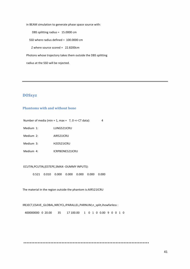
in BEAM simulation to generate phase space source with:

DBS splitting radius = 15.0000 cm

SSD where radius defined = 100.0000 cm

Z where source scored = 22.8200cm

Photons whose trajectory takes them outside the DBS splitting

radius at the SSD will be rejected.

DOSxyz

Phantoms with and without bone

Number of media (min = 1, max = 7, 0 => CT data): 4

Medium 1: LUNG521ICRU

Medium 2: AIR521ICRU

Medium 3: H2O521ICRU

Medium 4: ICRPBONE521ICRU

ECUTIN,PCUTIN,(ESTEPE,SMAX--DUMMY INPUTS):

0.521 0.010 0.000 0.000 0.000 0.000 0.000

The material in the region outside the phantom is:AIR521ICRU

IREJECT,ESAVE_GLOBAL,NRCYCL,IPARALLEL,PARNUM,n_split,ihowfarless :

400000000 0 20.00 35 17 100.00 1 0 1 0 0.00 9 0 0 1 0

*******************************************************************************

42

================================================================================


================================================================================


Photon transport cutoff(MeV) 0.1000E-01

Pair angular sampling SIM



Bound Compton scattering OFF



Atomic relaxations OFF

Photoelectron angular sampling OFF

Electron transport cutoff(MeV) 0.5210

Bremsstrahlung cross sections BH

Bremsstrahlung angular sampling SIM

Spin effects On


Maxium electron step in cm (SMAX) 5.000



Boundary crossing algorithm PRESTA-I



43

================================================================================

Medium AE AP

LUNG521ICRU 0.521 0.010

AIR521ICRU 0.521 0.010

H2O521ICRU 0.521 0.010

ICRPBONE521ICRU 0.521 0.010

No range rejection.

***************************************************************

Clinical Cases

CT Phantom summary:

NMED = 4

media:

AIR521ICRU

LUNG521ICRU

ICRUTISSUE521ICRU

ICRPBONE521ICRU

Densities range from 0.00100 - 2.08800 g/cc

44

ECUTIN,PCUTIN,(SMAX--DUMMY INPUT):

0.521 0.010 0.000

The material in the region outside the phantom is vacuum.

The thickness of this region (in x, y & z direction) is: 50.000 cm

NCASE,IWATCH,TIMMAX,INSEED1,INSEED2,BEAM_SIZE,ISMOOTH,IRESTART,IDAT,

IREJECT,ESAVE_GLOBAL,NRCYCL,IPARALLEL,PARNUM,n_split,ihowfarless:

480000000 0 100.00 33 99 100.00 1 0 1 0 0.00 9 0 0 1 0

45

References

1 Inhomogeneity correction and the analytic anisotropic algorithm, Don Robinson, Journal of applied clinical

medical physics, Volume 9 number 2, Spring 2008

2 Dosimetric validation of the anisotropic analytical algorithm for photon dose calculation: fundamental

characterization in water, Antonella Fogliata et al, Phys. Med. Biol. 51, February 2006

3 Dosimetric verification of the analytical anisotropic algorithm for radiotherapy treatment planning. C. Bragg,

and J. Conway, Radiotherapy and Oncology 81, 2006

4 Evaluating the Anisotrpic Analatical Algorithm (AAA) for 6 MV photon energy, Anders Josefsson, Master of

Science Thesis, Department of Radiation Physics Göteborg University, 2008

5 Monte Carlo Simulations of a Varian 600C Accelerator, Elin Haglund, Master of Science Thesis, Department of

Radiation Physics Göteborg University, 2006

6 BEAMnrc Users’s Manual, D. W. Rogers, B Walters and I. Kawrakow, Ionizing Radiation Standards Group,

Institute for National Measurement Standards, National Research Council Canada

7 Efficient photon beam dose calculations using DOSXYZnrc with BEAMnrc, I. Kawrakow and B. R. B. Walters,

Med. Phys. 33 (8), August 2006

8 AAA Photon Dose Calculation Model in Eclipse, Janne Sievinen, Waldemar Ulmer, Wolfgang Kassel, RAD

#7170, 2005

9 Testing of the analytical anisotropic algorithm for photon dose calculation, Ann van Esch et al, Med. Phys. 33,

November 2006

10 Converting absorbed dose to medium to absorbed dose to water for Monte Carlo based photon beam dose

calculations, J.V.Siebers et al, Phys. Med. Biol. 45, April 2000

11 Monte Carlo evaluation of the AAA treatment planning algorithm in a heterogeneous multilayer phantom

and IMRT clinical treatments for an Electa SL25 linear accelerator, E. Sterpin et al, Med. Phys. 34, May 2007

evaluation of the anisotropic analytical algorithm aaa … abstract the aim of this thesis is to...

Documents