evaluation of surfactant flooding for eor on the norne ... · eclipse 100 is used as simulation...
TRANSCRIPT

Evaluation of Surfactant Flooding for EOR on the Norne Field, C-segment
Kristine Nielsen
Master of Science in Engineering and ICT
Supervisor: Jon Kleppe, IPT
Department of Petroleum Engineering and Applied Geophysics
Submission date: June 2012
Norwegian University of Science and Technology


I
Abstract The world’s energy demand is constantly increasing. It offers a problem when hydrocarbons
both are the most energy efficient source known in combination with being a limited resource.
This motivates to increase the recovery from existing oil fields by means of EOR methods.
Surfactant flooding is such a method for enhancing the oil production from an oil field.
The Norne field is located in the North Sea. It is divided into four segments where the
C-segment is the focus area of this report. The production of oil started in 1997 and the
production is now declining. Water is being injected, however, to extract more oil tertiary
recovery is necessary. Surfactants aim to enhance the oil recovery by lowering the interfacial
tension between oil and water and hence lower the capillary pressure. This will mobilize the
residual oil and make it possible to produce.
Surfactant flooding can be an effective technique to boost the recovery, but there are several
challenges to overcome. These challenges include loss of surfactants to the formations,
facility and costs. The Norne C-segment being an offshore field represents an extra challenge.
Eclipse 100 is used as simulation tool to model the surfactant flooding. Prior to implementing
the surfactant model, history matching was performed. This was to calibrate the model in
order to ensure a better prediction of the activity in the reservoir. After implementing the
surfactant model, four different cases was evaluated to find the optimum injection strategy.
The cases include the injection into different formations, the use of different wells, and
alteration of concentration and injection period. An economical evaluation was performed
based on the results.
The results from the simulations were somewhat surprising and unexpected. Despite being a
suitable candidate through screening, surfactant flooding is not a feasible method to use at the
Norne C-segment.

II

III
Sammendrag Verdens energibehov er stadig økende. Når man tar i betraktning at hydrokarboner både er
den mest energieffektive kilden til energi i tillegg til å være ikke-fornybar representerer det en
utfordring. Dette motiverer til å øke utvinningen fra eksisterende oljefelt ved hjelp av EOR
metoder. Injeksjon av surfektanter i reservoaret er en slik metode for å øke utvinningen.
Norne-feltet ligger i Nordsjøen. Det er inndelt i fire segmenter der C-segmentet er
fokusområdet i denne rapporten. Produksjonen av olje startet i 1997 og er nå avtagende. Selv
om vann injiseres opprettholdes ikke trykket i reservoaret på det nødvendige nivået for å sikre
produksjon. Ved å injisere surfektanter i reservoaret vil grenseflatespenningen mellom vann
og olje senkes. Det kapillære trykket i porerommet vil som følge av dette bli lavere, dette vil
føre til mobilisering av residual olje.
Injeksjon av surfektanter kan være en svært effektiv metode for å øke utvinningen, men det er
flere utfordringer som må tas hensyn til. Blant slike utfordringer nevnes tap av surfektanter til
formasjonen, logistikk og gjennomføring samt økonomi. At C-segmentet på Norne er
lokalisert offshore byr på en ekstra utfordring.
Simuleringsprogrammet Eclipse 100 blir brukt som verktøy for å modellere effekten av
surfektanter i reservoaret. Før gjennomføring ble det utført historietilpasning for å kalibrere
modellen bedre. Dette ble utført for å bedre predikere aktiviteten i reservoaret. Etter å ha
implementert surfektantene i reservoaret ble fire forskjellige caser evaluert for å finne den
beste strategien for injeksjon. Casene inkluderte evaluering av formasjon til injisering, valg av
brønn, og endring i både konsentrasjon og lengde på injeksjonsintervallet. En enkel
økonomisk analyse ble utført på grunnlag av resultatene.
Resultatene var noe avvikende og overraskende i forhold til forventingene. Til tross for å bli
karakterisert som en passende kandidat for surfektantinjeksjon, er det ikke lønnsomt å bruke
denne metoden på C-segmentet til Norne.

IV

V
Preface This report is the result of my master thesis, which all graduates at Norwegian University of
Science and Technology execute prior to their graduation. It is an extension of my in-depth
project “Introduction to Surfactant Flooding for EOR on the Norne Field, C-segment”, and
some of the chapters regarding theory are from this previous work. The process of history
matching, presented in chapter 4, was executed in close collaboration with Anders
Abrahamsen.
Firstly I would like to address appreciation and gratitude to my supervisor Professor Jon
Kleppe at NTNU for his help and support during my work. I would also like to thank Richard
Rwechungura, Jan Ivar Jensen and Mehran Namani at NTNU for their support and advice.
Further I would like to thank Sindre Lillehaug and Bjørn Tore Samuelsen from Statoil’s
Norne team in Harstad for their assistance. I am grateful to Espen Kowalewski, Vegard Kippe
and Kristian Sandengen from Statoil who kindly answered questions via email. Finally, I
would like to thank the Center for Integrated Operations at NTNU, Statoil ASA as operator on
Norne, Petoro and ENI as partners for releasing data regarding the Norne field.
In addition I would like to thank my fellow student colleagues for support and good
discussions. I am also grateful for the unconditional support from my family during my
studies.
Trondheim, 2012
Kristine Nielsen [email protected]

VI

VII
Table of Contents
Abstract .................................................................................................................................................... I
Sammendrag ........................................................................................................................................... III
Preface ..................................................................................................................................................... V
List of Figures ........................................................................................................................................ XI
List of tables ......................................................................................................................................... XIII
1. Introduction ..................................................................................................................................... 1
2. Enhanced Oil Recovery – EOR ....................................................................................................... 3
2.1 Objective and principle of EOR .............................................................................................. 4
3. Norne field ....................................................................................................................................... 7
3.1 General .................................................................................................................................... 7
3.2 Geology ................................................................................................................................... 9
3.2.1 Ile formation .................................................................................................................... 9
3.2.2 Tofte formation ................................................................................................................ 9
3.3 Reservoir communication ...................................................................................................... 10
3.4 Drainage strategy ................................................................................................................... 11
3.5 EOR potential ........................................................................................................................ 12
3.6 Screening ............................................................................................................................... 13
3.7 The Norne reservoir model .................................................................................................... 14
4. History matching ........................................................................................................................... 17
4.1 Preparation of the model ....................................................................................................... 17
4.2 Workflow ............................................................................................................................... 19
4.3 Results and discussion ........................................................................................................... 23
5 Surfactant flooding ........................................................................................................................ 27
5.1 Characterization of surfactants .............................................................................................. 28
5.1.1 Hydrophile-Lipophile Balance (HLB) .......................................................................... 28
5.1.2 Critical Micelle Concentration (CMC) .......................................................................... 28
5.1.3 Solubilization Ratio ....................................................................................................... 29
5.2 Phase behavior ....................................................................................................................... 29
5.2.1 Phase behavior test ........................................................................................................ 29
5.2.2 Salinity ........................................................................................................................... 31
5.2.3 Temperature ................................................................................................................... 33
5.2.4 Oil composition ............................................................................................................. 33
VIII
5.3 Flooding of the reservoir ....................................................................................................... 33
5.4 The effects of surfactants....................................................................................................... 34
5.4.1 Capillary Number .......................................................................................................... 35
5.4.2 Wettability ..................................................................................................................... 37
5.4.3 Relative permeability..................................................................................................... 38
5.5 Challenges ............................................................................................................................. 38
5.5.1 Adsorption ..................................................................................................................... 39
5.5.2 Precipitation ................................................................................................................... 40
5.5.3 Economy ........................................................................................................................ 41
5.5.4 Field location ................................................................................................................. 41
5.6 Selection of surfactant ........................................................................................................... 41
6 Reservoir simulation ...................................................................................................................... 43
6.1 Eclipse 100 ............................................................................................................................ 43
6.2 The surfactant model ............................................................................................................. 43
6.3 Input values used in the surfactant model ............................................................................. 43
6.4 Economic model .................................................................................................................... 45
6.5 Procedure for simulation ....................................................................................................... 45
6.6 Simulation Cases ................................................................................................................... 46
7 Results from the simulation ........................................................................................................... 49
7.1 Case 1 – Formation selection ................................................................................................ 49
7.2 Case 2 – Well selection ......................................................................................................... 50
7.3 Case 3 – Surfactant concentration ......................................................................................... 53
7.4 Case 4 – Slug size .................................................................................................................. 54
8 Analyses and Discussion ............................................................................................................... 57
Case 1 – Formation selection ............................................................................................................ 57
Case 2 – Well selection ..................................................................................................................... 58
Case 3 – Surfactant concentration ..................................................................................................... 59
Case 4 – Slug size .............................................................................................................................. 59
Validation of data and the reservoir model ....................................................................................... 60
General .............................................................................................................................................. 61
9 Conclusion ..................................................................................................................................... 63
10 Uncertainties .............................................................................................................................. 65
11 Recommended further work ...................................................................................................... 67
12 Nomenclature ............................................................................................................................ 69

IX
13 References ................................................................................................................................. 71
Appendices ............................................................................................................................................ 75
A. Figures related to the reservoir model ........................................................................................... 75
B. Screening table .............................................................................................................................. 79
C. ECLIPSE 100 ................................................................................................................................ 81
D. Surfactant model............................................................................................................................ 83
The Capillary Number ....................................................................................................................... 83
Relative Permeability Model ............................................................................................................. 83
Capillary Pressure .............................................................................................................................. 83
Water PVT Properties ....................................................................................................................... 84
Adsorption ......................................................................................................................................... 84
E. Keywords in the Surfactant Model ................................................................................................ 85
SURFACT ......................................................................................................................................... 85
SURFST ............................................................................................................................................ 85
SURFVISC ........................................................................................................................................ 85
SURFCAPD ...................................................................................................................................... 85
SURFADS ......................................................................................................................................... 85
SURFROCK ...................................................................................................................................... 85
WSURFACT ..................................................................................................................................... 86
F. Surfactant input file ....................................................................................................................... 87
G. Prediction input file ....................................................................................................................... 89
H. Group input file ............................................................................................................................. 97
I. Region input file ............................................................................................................................ 99
J. Production rates and NPV ........................................................................................................... 101
K. Adsorption ................................................................................................................................... 117

X

XI
List of Figures
Figure 3.1 - The location of the Norne Field (Statoil, 2010). .................................................... 7
Figure 3.2 - The floating production and storage vessel at Norne (Offshore Technology,
2011). .......................................................................................................................................... 8
Figure 3.3 - The tilting structure and the layering of Norne (Verlo, 2008). ............................ 10
Figure 3.4 - Draining pattern of the Norne field (Verlo, 2008). .............................................. 12
Figure 3.5 - a) The remaining amount of easy oil b) The EOR potential. .............................. 13
Figure 3.6 - The full field Norne Model. .................................................................................. 14
Figure 3.7 - The ECLIPSE model of the C-Segment. .............................................................. 15
Figure 4.1 - Field production rate vs. historical production data. ............................................ 18
Figure 4.2 - Group production rate vs. historical production rate for the group. ..................... 18
Figure 4.3 - Local changes in layer 8; light green indicates low case area. ............................. 21
Figure 4.4 - Local changes in layer 11; light green indicates low case area and dark green
indicates high case area. ........................................................................................................... 22
Figure 4.5 - Local changes in layer 15; dark green indicates high case area. .......................... 22
Figure 4.6 - Water Cut, Initial model vs. new model vs. history. ............................................ 23
Figure 4.7 - Oil Production Rate. Initial model vs. new model vs. history. ............................. 24
Figure 4.8 - Water Cut well B-2H ............................................................................................ 25
Figure 4.9 - GOR well B-4H. ................................................................................................... 26
Figure 5.1 - The molecule structure of a surfactant ................................................................. 27
Figure 5.2 - Flow chart of how the phase behavior tests are performed. ................................. 30
Figure 5.3 - Illustrating the Pc equation (Skjæveland & Kleppe, 1992). ................................. 34
Figure 5.4 - Three phases in the imbibition of oil in a system of two pores in three stages; a, b
and c. ........................................................................................................................................ 35
Figure 5.5 - Capillary Desaturation Curve (CDC) (Skjæveland & Kleppe, 1992). ................. 36
Figure 5.6 - Wettability (Abdallah, et al., 2007). ..................................................................... 37
Figure 5.7 - Illustrating how the head groups cling to the surface in the phenomena of
adsorption (Dang, et al., 2011). ................................................................................................ 39
Figure 5.8 - Adsorption curve (Skjæveland & Kleppe, 1992). ................................................ 40
Figure 7.1 - Incremental Cumulative Oil production for Case 1. ............................................ 49
Figure 7.2 - Total adsorption of surfactants in Case 1. ............................................................ 50
Figure 7.3 - Incremental Cumulative Oil production for Case 2. ............................................ 51

XII
Figure 7.4 - Propagation of surfactants. ................................................................................... 52
Figure 7.5 - Incremental Cumulative Oil production for Case3. ............................................. 54
Figure 7.6 - Incremental Cumulative Oil production for Case 4a. ........................................... 55
Figure 7.7 - Incremental Cumulative Oil production for Case 4b. .......................................... 56
Figure A.1 - Illustration of the Norne field, white lined are indicating faults ......................... 75
Figure A.2 - Depicts the reservoir faulting. Numbers starting with C is located in the C-
segment ..................................................................................................................................... 75
Figure A.3 - Cross-section of the full field model, C-segment indicated with dotted line ...... 76
Figure A.4 - Coarsed model of the C-segment ......................................................................... 76
Figure A.5 - Hydrocarbon composition at the Norne Field (Kalsnæs, 2010). ......................... 77
Figure B.1 - Depicts the screening table (Taber, et al., 1997). ................................................ 79

XIII
List of tables
Table 3.1 - Shows the oil and gas properties in the reservoir. (Norwegian Petroleum
Directorate, 2011). ...................................................................................................................... 8
Table 3.2 - Summarizes the important key parameters in Norne (Maheshwari, 2011), (Lind, et
al., 2001). .................................................................................................................................. 11
Table 4.1 - Formations and corresponding layers and barriers. ............................................... 19
Table 5.1 - Shows the advantages and the disadvantages for the different types of
microemulsions (Sheng, 2011). ................................................................................................ 32
Table 7.1 - Total oil production, increase in total production, NPV and adsorption for Case 2.
.................................................................................................................................................. 51
Table 7.2 - Total oil production, increase in total production, NPV and adsorption for Case 3.
.................................................................................................................................................. 53
Table 7.3 - Total oil production, increase in total production, NPV and adsorption for Case 4a.
.................................................................................................................................................. 55
Table 7.4 - Total oil production, increase in total production, NPV and adsorption for Case 4b.
.................................................................................................................................................. 56

XIV
1
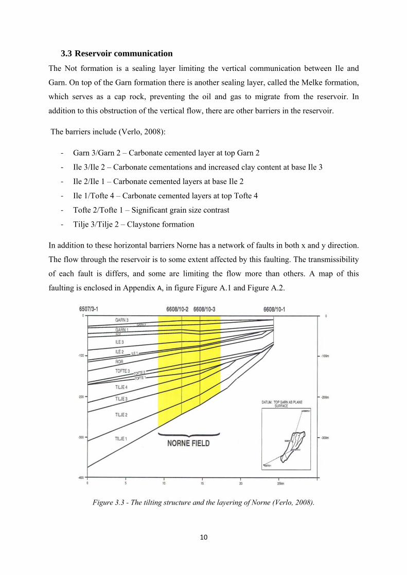
1. Introduction
Hydrocarbons are still the largest and most effective source of energy known today (IEA,
2011). As the need for energy worldwide constantly is growing there is a rising demand for
oil and gas. At the same time the world’s production of hydrocarbons is declining. This
represents a challenge when knowing that the resources are limited and new discoveries are
rare. To be able to address the demand for energy, new technology for enhancing the oil
recovery of existing fields is a necessity.
The average recovery factor from oil fields after abandonment is around 30-40% (TOTAL,
2008). For the Norwegian continental shelf it is a bit higher, around 46% (Olje- og
energidepartementet, utvinningsutvalget, 2010). These numbers indicate that the residual
amount of oil is around 50%. To extract this oil, methods for enhanced oil recovery (EOR) are
used.
There is a big portfolio of different EOR methods aiming differently to extract oil from the
reservoir. Surfactant flooding is such a method. It can be compared to soap in in the way it
targets the extraction of residual oil. No methods for EOR are commercially used on the
Norwegian continental shelf today. This is partly due to the high recovery factor, the high cost
of EOR-methods and to the new findings on the shelf. The only experiment of surfactant
flooding outside laboratory in Norway is two single well studies on Gullfaks and Oseberg
(Olje- og energidepartementet, utvinningsutvalget, 2010). Both projects gave increased
recovery, however they were not economically feasible. As EOR methods tend to be costly to
implement it requires a high and stable oil price in order to provide a positive return.
This study is an extension of the project “Introduction to Surfactant Flooding for EOR on the
Norne Field, C-segment”, and it aims to explain the method of injecting surfactants into the
C-segment of the Norne field in order to recover the residual oil. Prior to the simulation of
this, the reservoir model will be history matched to achieve the most accurate results. The
simulation program Eclipse 100 will be used as a tool for modeling surfactant flooding of the
reservoir. An economic analysis will also be performed to determine the feasibility of such a
project.

2

3
2. Enhanced Oil Recovery – EOR
This chapter is originally from the pre-study; “Introduction to Surfactant Flooding for EOR on
the Norne Field, C-segment” by Kristine Nielsen.
The production of hydrocarbons from a reservoir is typically divided into three stages;
primary, secondary and tertiary recovery.
- Primary recovery is also called natural depletion. This denotes the production derived
by the natural pressure difference in the reservoir and the bore hole. During
production, the pressure in the reservoir will decline. This results in lower production.
To maintain the production it is necessary to maintain the pressure. The recovery rate
after natural depletion is on average 46% on the Norwegian shelf (Kristensen, 2011).
- Secondary recovery aims to maintain pressure by injecting non-alien fluids or gasses
into the reservoir. The fluids and gases are typically water and natural gas.
- Tertiary recovery denotes the production that is done after secondary recovery no
longer is successful. This is done by injecting alien fluids or gases into the reservoir.
This is in literature also referred to Incremental/Improved Oil Recovery (IGR) and
Enhanced Oil Recovery (EOR) (UNSW, 2011).
There are many techniques for EOR, which all aim to improve on the recovery. The term
recovery can be divided into microscopic and macroscopic recovery. Some of the methods
seek to improve on the recovery by increasing microscopic displacement and others by
increasing macroscopic displacement. Some techniques aim to increase both.
The EOR methods are typically divided into solvent-, thermal- and chemical methods;
- Solvent methods denote different strategies of injecting gas into the reservoir. This is
typically CO2, nitrogen or flue gas (UNSW, 2011).
- Thermal methods are techniques where either hot water or steam is injected to increase
the reservoir temperature. This aims to increase the oil viscosity which makes the oil
more mobile and in turns provide an increase in the production.
4
- Chemical methods refer to techniques were chemicals are injected. The chemicals can,
depending on the particular chemical, both aim to increase the microscopic and
macroscopic displacement. Surfactants, polymers and alkalines are examples of such
chemicals. These may be used separately or combined in order to boost the
production.
Techniques for EOR have been studied at a broad scale. However, no methods are
commercially used in the North Sea (Awan, et al., 2006).
2.1 Objective and principle of EOR
As stated the objective of EOR is to increase the microscopic or macroscopic displacement
efficiency, or both, and hence the production of hydrocarbons.
The microscopic displacement efficiency (ED) denotes the displacement on a pore-scale level
and is closely related to the residual oil saturation, Sor (Green & G Paul, 1998). The amount of
oil trapped in the reservoir, after primary and secondary recovery, is on a microscopic level
controlled by the capillary pressure and thus the interfacial tension (IFT). These two
parameters are correlated and proportional. By decreasing the IFT the capillary pressure will
decrease, this makes the residual oil mobile and hence possible to produce. The capillary
pressure and the IFT are linked together in Laplace’s Equation which is further explained in
Chapter 5.4, where the effects of surfactants are described.
The macroscopic displacement is called the volumetric sweep efficiency and is strongly
dependent on the mobility between the phases in the reservoir (Johannesen & Graue, 2007).
The mobility is controlled by the viscosity of the specific phase. When the residual amount of
oil is trapped in the reservoir due to low mobility of the displacing phase, the viscous forces
are the dominating forces (Dr.Tran, 2006). The volumetric sweep (EV) is defined as the
product between the areal (EA) and the vertical (EI) sweep efficiency. Areal sweep denotes the
area swept by the injecting phase divided by the whole area. Vertical sweep refers to the
fraction of the vertical area swept by the injecting phase (Dr.Tran, 2006), (Sehbi, et al., 2001).
= ∗ (2.1)
An important value called the capillary number (NC) designate whether the capillary forces or
the viscous forces dominate in the reservoir. The value is defined as (Johannesen & Graue,
2007):

5
= (2.3)
Where v is the Darcy velocity, μ is the viscosity of the displacing fluid which is water
containing surfactant in this case and σ is the interfacial tension between the displacing and
displaced phase. The value of this number gives an indication of which displacement
efficiency important to target in order to improve on the recovery. The reservoir is dominated
by the capillary forces if NC < 10-5, the amount of trapping is normally high at this value
(Dr.Tran, 2006). To improve on the recovery it will be necessary to lower the IFT to increase
NC and then increase EV by improving the mobility ratio (M). If the value of NC > 10-5 the
viscous forces dominate in the reservoir and thus the residual oil is trapped due to mobility
issues. It will then be adequate to improve the mobility ratio to improve on the recovery.
The mobility ratio is defined as (Johannesen & Graue, 2007):
= = (2.4)
Where λ denotes the mobility, kr denotes the relative permeability and μ denotes the viscosity.
The mobility ratio characterizes how the displacing and displaced phase flows in relation to
each other. It is desirable to keep M ≥ 1 (Lien, 2008). This indicates that the displaced phase
moves more rapidly than the displacing fluid and thus the front is stable. If M < 1 undesirable
results like viscous fingering may occur (Lien, 2008). Viscous fingering denotes when the
displacing phase moves more quickly and penetrates the displaced phase. This results in an
early breakthrough of the displacing phase, which in turns decreases the overall recovery. In
order to keep the mobility ratio at a low level the viscosity of the phases must be monitored
and altered if necessary. Lowering the IFT or mobility ratio is by means of EOR methods.

6

7
3. Norne field
This chapter is based on the pre-study; “Introduction to Surfactant Flooding for EOR on the
Norne Field, C-segment” by Kristine Nielsen.
3.1 General
The Norne Field is located on the Norwegian continental shelf about 200 km from the main
land between Sandnessjøen and Brønnøysund. Its position is indicated with a red mark in
Figure 3.1. The specific location is at block 6608/10 and 6608/11. The operator of the field is
Statoil ASA. It is controlled from Harstad in Northern Norway by Statoil with Petoro, with a
share of 54%, and Eni Norway, with a share of 6.9%, as partners (Norwegian Petroleum
Directorate, 2011).
Figure 3.1 - The location of the Norne Field (Statoil, 2010).
The field was discovered in 1991, drilling started in 1996 and production a year after that in
1997. It is developed using a floating production and storage vessel which is connected to
seven subsea templates, as illustrated in Figure 3.2 (Lind, et al., 2001). This vessel has a
processing plant aboard and storage tanks for stabilized oil (Statoil, 2010). Norne is divided
into two divisions, the Main Structure containing the C-, D- and E-segment and the Northeast
segment containing the G- segment. Faulting of the whole reservoir determines the
demarcation of the different segments. Faulting is discussed in chapter 0.
The original oil in place (OOIP) and original gas in place (OGIP) was calculated to be 156.0 x
106 Sm3 and 28.90 x 10⁹ Sm3 respectively (Lind, et al., 2001), whilst the recoverable oil and
gas in place was calculated to be 93.40 x 10⁶ Sm3 and 11.70 x 10⁹ Sm3. Recoverable oil gas is
the oil the volumes possible to produce. Table 3.1 summarizes this.

8
Table 3.1 - Shows the oil and gas properties in the reservoir. (Norwegian Petroleum Directorate,
2011).
Figure 3.2 - The floating production and storage vessel at Norne (Offshore Technology, 2011).
Orig. in place Recoverable Remaining Orig. in place Recoverable Remaining156 93,4 8,8 28,9 11,7 0,9
Oil Gas
[mill. Sm3] [bill. Sm3]

9
3.2 Geology
The reservoir is structured as depicted in Figure 3.3. The formations are mainly sandstone
from the Middle to Upper Jurassic era. The whole reservoir is measured to be approximately
224 meters thick, and is situated at a depth of 2500-2700 meters. This exposes the reservoir to
digenetic processes e.g. mechanical compaction which in turn will reduce the quality of the
reservoir. The average porosity is in the range of 25-30%. The permeability differs from 20-
2500mD. The initial pressure was determined to be 273bars (Verlo, 2008). Table 3.2
summarizes the key data.
There are four major formations in the Norne reservoir called; Garn, Ile, Tofte and Tilje.
Between Ile and Garn there is also a thin layer called the Not formation. About 80% of the oil
is assumed to be situated in the Ile and Tofte formations, and the majority of the gas in the
Garn layers.
3.2.1 Ile formation
The Ile formation is 32-40m thick and is defined between layer 5 and 11 in the reservoir
model. The formation is sandstone deposited in a semi-marine environment during the late
Toarcian to Aalenian age in Mesozoic era (Directorate, 2012). There are representations of
tidal-influenced deltas and coastline settings (Directorate, 2012). The formation is divided
into three zones according to characteristic features particular layers. Zone 1 is the lower layer
of the three, both this and layer two consist of fine to very fine grained sandstone. The upper
zone is coarser than the underlying zones and has slightly poorer reservoir quality (Verlo,
2008).
3.2.2 Tofte formation
The Tofte formation is also sandstone deposited in a semi-marine environment, but during the
late Troarcian to Pliensbachian geologic age period (Directorate, 2012). In the reservoir
model Tofte is defined from layer 12 through layer 18. As with Ile it is divided in three zones.
The zones are coarsening upwards with medium to coarsed sandstone in zone 1, fine grained
in zone 2 and very fine to fine grained sandstone in zone 3.
10
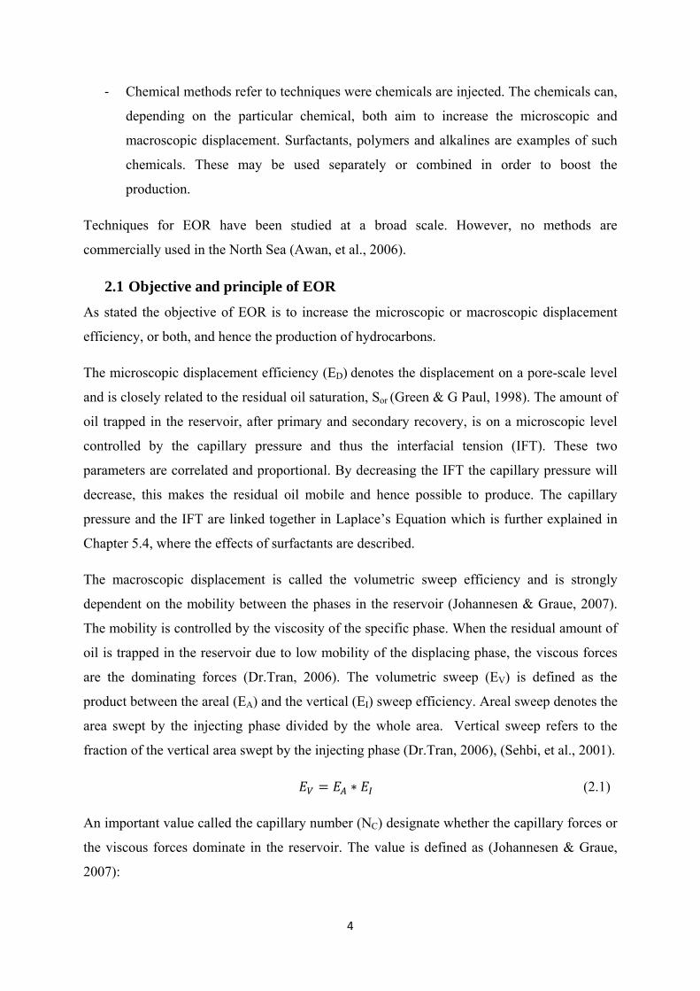
3.3 Reservoir communication
The Not formation is a sealing layer limiting the vertical communication between Ile and
Garn. On top of the Garn formation there is another sealing layer, called the Melke formation,
which serves as a cap rock, preventing the oil and gas to migrate from the reservoir. In
addition to this obstruction of the vertical flow, there are other barriers in the reservoir.
The barriers include (Verlo, 2008):
- Garn 3/Garn 2 – Carbonate cemented layer at top Garn 2
- Ile 3/Ile 2 – Carbonate cementations and increased clay content at base Ile 3
- Ile 2/Ile 1 – Carbonate cemented layers at base Ile 2
- Ile 1/Tofte 4 – Carbonate cemented layers at top Tofte 4
- Tofte 2/Tofte 1 – Significant grain size contrast
- Tilje 3/Tilje 2 – Claystone formation
In addition to these horizontal barriers Norne has a network of faults in both x and y direction.
The flow through the reservoir is to some extent affected by this faulting. The transmissibility
of each fault is differs, and some are limiting the flow more than others. A map of this
faulting is enclosed in Appendix A, in figure Figure A.1 and Figure A.2.
Figure 3.3 - The tilting structure and the layering of Norne (Verlo, 2008).

11
Table 3.2 - Summarizes the important key parameters in Norne (Maheshwari, 2011), (Lind, et al., 2001).
Properties Units Norne Main Structure
(C-, D- and E- segment)
Norne G-segment
Fluid
Initial pressure(Pi) bar 273.2 273.2
Bubble point pressure(PBO) bar 251 216
Gas oil ratio(GOR) Sm3/Sm3 111 96
Oil formation factor at bubble point(Bo,BO) Rm3/Rm3 1.347 1.30
Oil viscosity at bubble point(μo, BO) cp 0.58 0.695
Oil density at bubble point(ρo, BO) g/cm3 0.712 0.729
API gravity ⁰ 32.7
Gas formation factor(Bg) Rm3/Rm3 4.74E-3
Reservoir
Formation type Sandstone
Initial temperature(T) ⁰C 98.3 98.3
Porosity(ϕ) % 25-30
Permeability(K) mD 20-2500
Depth(D) m 2500-2700
Thickness m 224
Oil saturation(So) % 35-92
3.4 Drainage strategy
In 2006 13 wells were situated in the C-segment at Norne, 9 producers and 4 injectors
(Kheradmand, 2011).
There are mainly horizontal producers at Norne. The first production wells drilled were
vertical; these have later been sidetracked to horizontal wells (Verlo, 2008). The original
drainage strategy was to inject gas into the gas cap and water into the water zone in order to
maintain the reservoir pressure. The discovery of the sealing Not formation led to the
abandonment of this strategy. It was instead decided to inject the gas into the water zone and
lower part of the oil zone (Lind, et al., 2001). In 2005 the injection of gas was stopped as
exportation of gas began. Oil was produced with water injection as the only driving
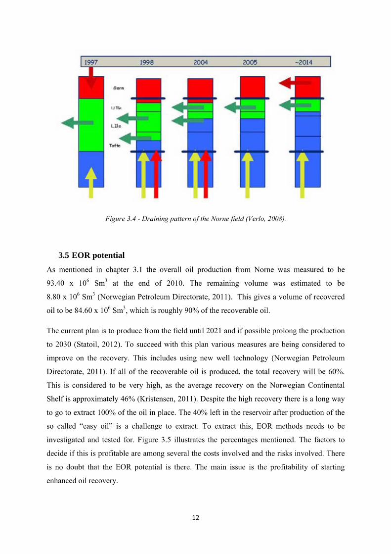
mechanism. Figure 3.4 illustrates the drainage strategy. The red color illustrates gas, green
color indicates oil, blue color for water. The yellow arrow illustrates injection of water, red
arrow illustrates injection of gas and the green arrow depicts production of gas.
12
Figure 3.4 - Draining pattern of the Norne field (Verlo, 2008).
3.5 EOR potential
As mentioned in chapter 3.1 the overall oil production from Norne was measured to be
93.40 x 10⁶ Sm3 at the end of 2010. The remaining volume was estimated to be
8.80 x 10⁶ Sm3 (Norwegian Petroleum Directorate, 2011). This gives a volume of recovered
oil to be 84.60 x 10⁶ Sm3, which is roughly 90% of the recoverable oil.
The current plan is to produce from the field until 2021 and if possible prolong the production
to 2030 (Statoil, 2012). To succeed with this plan various measures are being considered to
improve on the recovery. This includes using new well technology (Norwegian Petroleum
Directorate, 2011). If all of the recoverable oil is produced, the total recovery will be 60%.
This is considered to be very high, as the average recovery on the Norwegian Continental
Shelf is approximately 46% (Kristensen, 2011). Despite the high recovery there is a long way
to go to extract 100% of the oil in place. The 40% left in the reservoir after production of the
so called “easy oil” is a challenge to extract. To extract this, EOR methods needs to be
investigated and tested for. Figure 3.5 illustrates the percentages mentioned. The factors to
decide if this is profitable are among several the costs involved and the risks involved. There
is no doubt that the EOR potential is there. The main issue is the profitability of starting
enhanced oil recovery.

13
Figure 3.5 - a) The remaining amount of easy oil b) The EOR potential.
3.6 Screening
After having determined whether the potential for improving the oil recovery is of the right
scale, it is necessary to screen the field against the different EOR methods. As mentioned in
chapter 2 there are several different EOR methods. The process of finding the method best
suited for a particular reservoir is often based on a set of screening criteria developed by J.
Taber. These criteria are based on data from successful field projects and on the general
understanding of conditions that favors recovery from a reservoir. The properties often
considered most important are; API-Gravity, viscosity, composition, oil saturation, formation
type, net thickness, average permeability, depth and temperature (Taber, et al., 1997). In the
procedure of evaluating the field, the properties mentioned have a range of values for each
EOR method. The screening is not all black and white and there can be more than one suitable
method for a particular field, if so the cost aspect can determine a method. As new technology
continuously is being developed, some of the methods may prove to be successful even if it
does not agree with the screening model.
The key data from the Norne field in Table 3.2 was compared to the criteria in the screening
method developed by J. Taber. An overview of the screening criteria is found in Error!
Reference source not found. in Appendix 0. The evaluation immediately excluded the majority
of the methods. The methods micellar/polymer, ASP and alkaline and polymer flooding,
defined as 4 and 5 in Taber’s screening model, stood out as the best candidates. Overall, these
chemical EOR methods corresponded well with the defined values.
A sandstone reservoir is preferred in order to minimize the adsorption and loss of chemicals
(Michaels, et al., 1996). As Norne generally is a sandstone reservoir, it is a good match. The
API-gravity at Norne is 32,7° and above the desired 20° for chemical flooding. As for the
composition of hydrocarbons it is desirable to have light to intermediate hydrocarbons. An

14
overview of the hydrocarbon composition, shown in Figure A.5 in Appendix A, depicts that
this is the case for Norne. The viscosity of the oil distinguish the use of surfactants and
polymers in the reservoir. The oil viscosity for a surfactant flood should be less than 10cP and
preferably less than 3cP (Michaels, et al., 1996). This is to avoid the need for polymer drive.
In Norne the viscosity is 0,58cP and well below the desired value.
3.7 The Norne reservoir model
The model of the Norne field is originally developed by Statoil ASA, the version used in this
report was last edited in 2004 (Statoil, 2010). Prior to the simulation of surfactant flooding the
model needed to be history matched; this process is discussed in the next chapter.
The full field model of Norne, showed in Figure 3.6, consists of 46x112x22 grids with 49080
active grid cells. The C-segment is indicated with the circle in Figure 3.6 and in its entirety in
Figure 3.7. The C-segment consists of 19911 active grid cells (Kheradmand, 2011). The
model is coarsed meaning that cells have been merged together to make a more simplistic
model. Figure A.3 and Figure A.4 in Appendix A depict the cross-section of the full field
model and the C-segment. The procedure of coarsening the full field model it is done in a
matter which maintains the quality of the result. The actual procedure of how it is done is not
a subject in this report. The model has as previously mentioned 13 wells where 4 are injectors
and 9 are producers (Kheradmand, 2011).
Figure 3.6 - The full field Norne Model.

15
Figure 3.7 - The ECLIPSE model of the C-Segment.

16

17
4. History matching
History matching is a challenging task which aims to calibrate a reservoir model against
historical data for the particular field. Simulated values are compared to observed well and
reservoir performance. The difference between the two sets of results is evaluated. If the
difference is characterized to be significant, alterations are done to the reservoir model. Such
alterations involve changing reservoir parameters with the highest level of uncertainty. Once
the model is history matched the future behavior can be more accurately predicted.
History matching is normally done manually, meaning that the reservoir engineer is
evaluating the flow and changing parameters. To speed up this process, one may want to use a
computer assisted approach, where the computer simulates for different values within a set of
values defined beforehand. The history matching can also be performed solely by a computer,
however, this approach is commonly considered to be too inaccurate. In this work manual
history matching is performed.
In literature several outlines/sketches on how to best perform history matching are suggested.
These advised methods will possibly differ from each other (Carlson, 2003). Performing
history matching is complex, and the procedure is dependent on the characteristics of the
reservoir in question. Regardless of this, some general aspects can be emphasized as
important when performing history matching. Pressure and the translation of geological data
to the reservoir model are considered uncertain (Carlson, 2003), (Satter, et al., 2008).
4.1 Preparation of the model
Prior to history matching of the C-segment the model had to be adjusted to get the correct
flow curves. The model of the C-segment is a coarsened model of the whole Norne field.
Some wells, not located in the C-segment, are producing from and injecting into the C-
segment. This is a correct depiction of the situation considering pressure support, however
when working solely with the C-segment, these must be left out. The model in this project is
therefore a grouping of the wells only situated in the C-segment. The following figures
depicts the oil production rate prior to and after the grouping of the wells. The input file to
Eclipse showing the grouping of the wells is enclosed in Appendix H.

18
Figure 4.1 - Field production rate vs. historical production data.
Figure 4.2 - Group production rate vs. historical production rate for the group.
In Figure 4.1 the oil production is too low, especially from 2000 and until 2004, when
compared to the measured data. When the wells situated in the C-segment are compared to the
history, the match is improved, Figure 4.2 depicts this.
1997 1998 1999 1999 2000 2001 2001 2002 2003 2004 2004 2005 2006 2006
Year
0
10000
20000
30000
40000
(SM
3/D
AY)
Field Oil Production Rate Norne C-segment
Oil Production Rate Oil Production rate HISTORY
1997 1998 1999 1999 2000 2001 2001 2002 2003 2004 2004 2005 2006 2006
Years
0
5000
10000
15000
20000
25000
(SM
3/D
AY)
Group Oil Production Rate Norne C-segment
Oil Production Rate Oil Prroduction Rate HISTORY

19
4.2 Workflow
As previously mentioned, pressure is considered a parameter to be matched in an early stage
of the process (Satter, et al., 2008). The permeability is altered in order to change the pressure
(Gruenwalder, et al., 2007). However, no history data for the pressure in the C-segment of the
Norne field were available. In order to improve the reservoir model another aspect considered
highly uncertain were investigated, namely the integration between geology and the reservoir
model. This is an area likely to cause distance between real and calculated values (Carlson,
2003). Considering the amount of data available, the Norne team in Harstad advised to alter
the vertical barriers to match the model. For the C-segment of Norne there are as previously
mentioned four major formations (Garn, Ile, Tofte and Tilje) which further is divided into
subdivisions. A number of field-wide barriers is said to obstruct flow in the vertical direction
(Verlo, 2008). These were presented in Chapter 0, Table 4.1 depicts a recap.
Table 4.1 - Formations and corresponding layers and barriers.
Layer Formation
1 Garn 3 carbonate cemented layer @top of Garn2
2 Garn 2 3 Garn 1 4 NOT 5 Ile 2.2 6 Ile 2.1.3 7 Ile 2.1.2 8 Ile 2.1.1 carbonate cemented layer @base Ile 2.1.1
9 Ile 1.3 10 Ile 1.2 11 Ile 1.1 carbonate cemented layer @top Tofte 2.2
12 Tofte 2.2 13 Tofte 2.1.3 14 Tofte 2.1.2 15 Tofte 2.1.1 grain size contrast
16 Tofte 1.2.2 17 Tofte 1.2.1 18 Tofte 1.1
19 Tilje 4 20 Tilje 3 clay stone
21 Tilje 2 22 Tilje 1

20
The barriers between layer 1/2, 15/16, 18/19 and 20/21 were implemented in the original
reservoir model. The barrier between layers 8/9 and 11/12 were implemented in the process of
history matching.
These existing barriers are implemented in the reservoir model by using the keyword MULTZ
with a designated value in the GRID section. When the MULTZ keyword is used in the GRID
section in Eclipse the transmissibility values are set to the specified value. The alterations and
the implementation of the new barriers are done using the same keyword, but in the EDIT-
section. In the EDIT-section the MULTZ value is multiplied with the transmissibility
designated earlier. The transmissibility describes the ability of fluids to flow through the grid
blocks of the reservoir model.
History matching was performed in the following manner in this report:
1) The transmissibility of field wide barriers was given a low and a high case MULTZ
value. The cases were simulated.
2) After simulating these cases, the water cut and gas-oil ratio for each well were studied
and they were compared to the original reservoir values. The target was to define the
best case for each well. For some wells the performance were improved by the
modification to high case. Some showed improvement when using the low case value
of transmissibility, and some changed for the worse with either of the adjustments.
Layer 18 and 20 were eliminated for further analysis at this stage. This was due to
unchanged well performance with the alterations introduced.
3) As mentioned, the geology of the field is challenging to predict and translate into a
reservoir model. In accordance with this it is difficult to state whether the barriers are
field wide, or have local zones with different transmissibility. After step 2 each of the
layers were altered to have a local area of high case transmissibility over the wells that
favored this value, and the same approach for the wells that showed a better match for
the lower case. When the high or low value of the transmissibility between the layers
failed to show any improvement in the well performance the original values was kept.
Figure 4.3, Figure 4.4 and Figure 4.5, depicts these local changes.
21
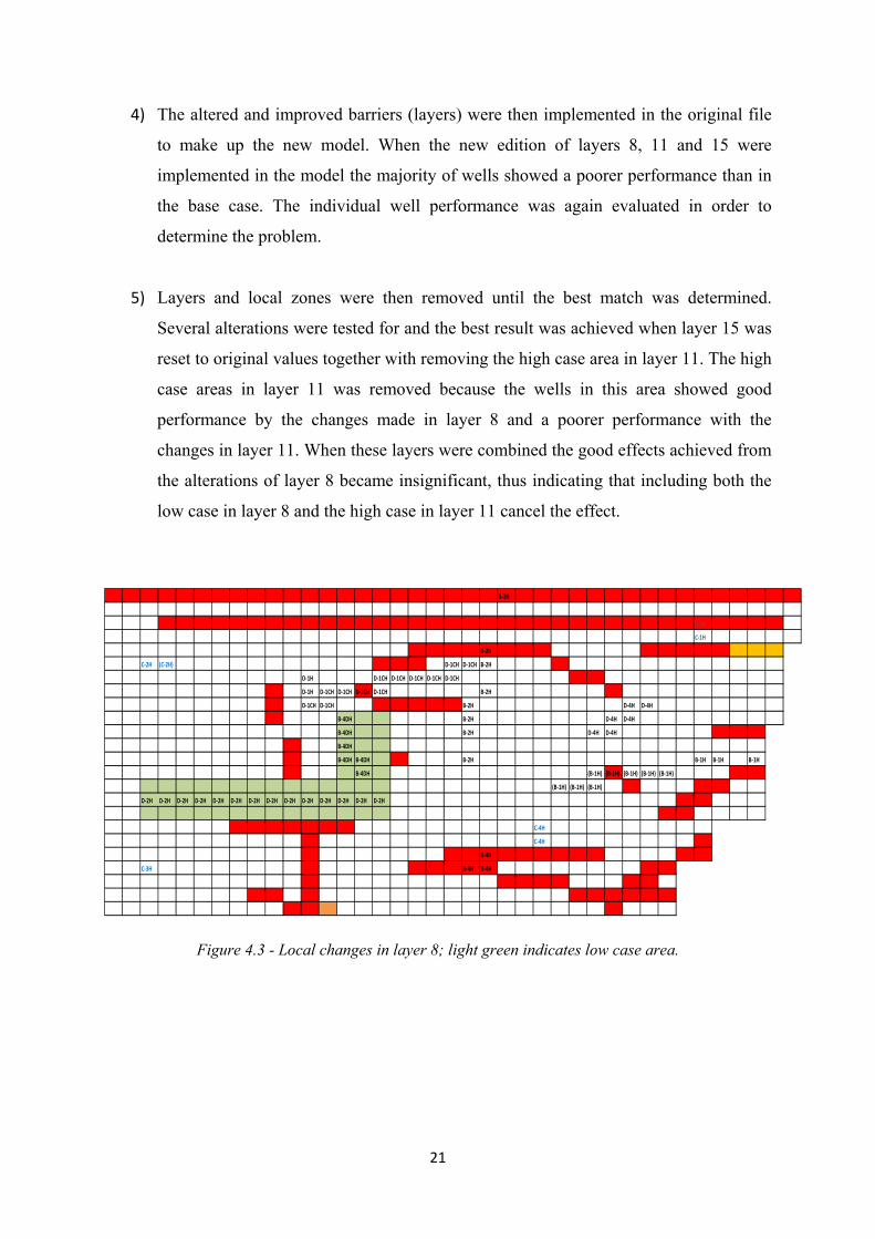
4) The altered and improved barriers (layers) were then implemented in the original file
to make up the new model. When the new edition of layers 8, 11 and 15 were
implemented in the model the majority of wells showed a poorer performance than in
the base case. The individual well performance was again evaluated in order to
determine the problem.
5) Layers and local zones were then removed until the best match was determined.
Several alterations were tested for and the best result was achieved when layer 15 was
reset to original values together with removing the high case area in layer 11. The high
case areas in layer 11 was removed because the wells in this area showed good
performance by the changes made in layer 8 and a poorer performance with the
changes in layer 11. When these layers were combined the good effects achieved from
the alterations of layer 8 became insignificant, thus indicating that including both the
low case in layer 8 and the high case in layer 11 cancel the effect.
Figure 4.3 - Local changes in layer 8; light green indicates low case area.
B-2H
C-1H
C-1H
B-2H
C-2H (C-2H) D-1CH D-1CH B-2H
D-1H D-1CH D-1CH D-1CH D-1CH D-1CH
D-1H D-1CH D-1CH D-1CH D-1CH B-2H
D-1CH D-1CH B-2H D-4H D-4H
B-4DH B-2H D-4H D-4H
B-4DH B-2H D-4H D-4H
B-4DH
B-4DH B-4DH B-2H B-1H B-1H B-1H
B-4DH (B-1H) (B-1H) (B-1H) (B-1H) (B-1H)
(B-1H) (B-1H) (B-1H)
D-2H D-2H D-2H D-2H D-2H D-2H D-2H D-2H D-2H D-2H D-2H D-2H D-2H D-2H
C-4H
C-4H
B-4H
C-3H B-4H B-4H

22
Figure 4.4 - Local changes in layer 11; light green indicates low case area and dark green indicates
high case area.
Figure 4.5 - Local changes in layer 15; dark green indicates high case area.
B-2H
C-1H
C-1H
B-2H
C-2H (C-2H) D-1CH D-1CH B-2H
D-1H D-1CH D-1CH D-1CH D-1CH D-1CH
D-1H D-1CH D-1CH D-1CH D-1CH B-2H
D-1CH D-1CH B-2H D-4H D-4H
B-4DH B-2H D-4H D-4H
B-4DH B-2H D-4H D-4H
B-4DH
B-4DH B-4DH B-2H B-1H B-1H B-1H
B-4DH (B-1H) (B-1H) (B-1H) (B-1H) (B-1H)
(B-1H) (B-1H) (B-1H)
D-2H D-2H D-2H D-2H D-2H D-2H D-2H D-2H D-2H D-2H D-2H D-2H D-2H D-2H
C-4H
C-4H
B-4H
C-3H B-4H B-4H
B-2H
C-1H
C-1H
B-2H
C-2H (C-2H) D-1CH D-1CH B-2H
D-1H D-1CH D-1CH D-1CH D-1CH D-1CH
D-1H D-1CH D-1CH D-1CH D-1CH B-2H
D-1CH D-1CH B-2H D-4H D-4H
B-4DH B-2H D-4H D-4H
B-4DH B-2H D-4H D-4H
B-4DH
B-4DH B-4DH B-2H B-1H B-1H B-1H
B-4DH (B-1H) (B-1H) (B-1H) (B-1H) (B-1H)
(B-1H) (B-1H) (B-1H)
D-2H D-2H D-2H D-2H D-2H D-2H D-2H D-2H D-2H D-2H D-2H D-2H D-2H D-2H
C-4H
C-4H
B-4H
C-3H B-4H B-4H
23
4.3 Results and discussion
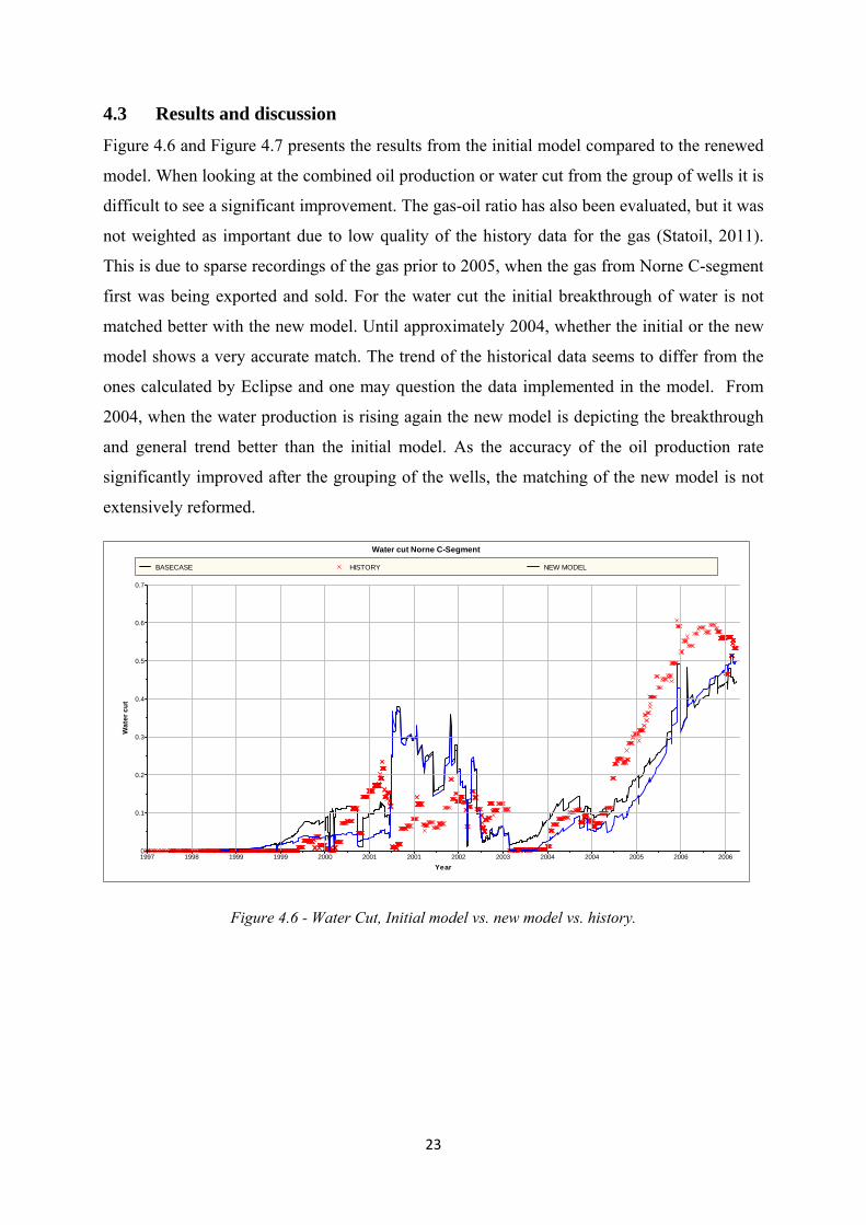
Figure 4.6 and Figure 4.7 presents the results from the initial model compared to the renewed
model. When looking at the combined oil production or water cut from the group of wells it is
difficult to see a significant improvement. The gas-oil ratio has also been evaluated, but it was
not weighted as important due to low quality of the history data for the gas (Statoil, 2011).
This is due to sparse recordings of the gas prior to 2005, when the gas from Norne C-segment
first was being exported and sold. For the water cut the initial breakthrough of water is not
matched better with the new model. Until approximately 2004, whether the initial or the new
model shows a very accurate match. The trend of the historical data seems to differ from the
ones calculated by Eclipse and one may question the data implemented in the model. From
2004, when the water production is rising again the new model is depicting the breakthrough
and general trend better than the initial model. As the accuracy of the oil production rate
significantly improved after the grouping of the wells, the matching of the new model is not
extensively reformed.
Figure 4.6 - Water Cut, Initial model vs. new model vs. history.
1997 1998 1999 1999 2000 2001 2001 2002 2003 2004 2004 2005 2006 2006
Year
0
0.1
0.2
0.3
0.4
0.5
0.6
0.7
Wat
er c
ut
Water cut Norne C-Segment
BASECASE HISTORY NEW MODEL

24
Figure 4.7 - Oil Production Rate. Initial model vs. new model vs. history.
The effect of the changes in the new model is more visible when studying the performance of
each well. To illustrate this, Figure 4.8 and Figure 4.9 shows the water cut curve for well B-
2H and the gas-oil ratio for well B-4H.
B-2H is a horizontal well situated in the middle of the reservoir and is perforated both in
layers 9 and 10. The water is delayed by the changes in transmissibility in the new model,
which is in accordance with the history. It may be questioned that the water is too obstructed
by the low case transmissibility in layer 11, however the improved match in the beginning
makes the new model the better choice. Figure 4.8 on the next panged depicts this.
1997 1998 1999 1999 2000 2001 2001 2002 2003 2004 2004 2005 2006 2006
Year
0
5000
10000
15000
20000
25000
(SM
3/D
AY)
Oil production rate Norne C-Segment
BASECASE HISTORY NEW MODEL

25
Figure 4.8 - Water Cut well B-2H
Well B-4H is also situated in the middle of the reservoir, south of B-2H and is perforated in
layer 13 through 15. This well does not have any water production. The new model gave a
considerably better match of the gas-oil ratio between 1997 until 1999. In this case the
historical data shows a different trend during 1999, this can be due to the mentioned
inaccuracy in the measured gas data. Figure 4.9 on the next page depicts this.
1997 1998 1999 1999 2000 2001 2001 2002 2003 2004 2004 2005 2006 2006
Year
0
0.1
0.2
0.3
0.4
0.5
0.6
0.7
0.8
Wat
er c
utWater Cut B-2H
BASECASE HISTORY NEW MODEL

26
Figure 4.9 - GOR well B-4H.
The workflow presented in this report is one of the many procedures tested in order to better
the match. As mentioned the pressure data was lacking. Due to this the main priority was to
alter the flow of fluids. Prior to consulting with Statoil in Harstad the focus was more on the
faults in the reservoir. Figure A.2 in Appendix A and the red lines in Figure 4.3 shows that
there are excessive faulting in the C-segment. These have different transmissibility values
which affects the horizontal flow. However, altering these values lacked to show any positive
results on the matching. This indicates that the process of history matching is a complex
procedure, particularly in a complex reservoir such as the C-segment. It was challenging to
make alterations that solely gave good results. The majority of the changes provided both
positive and negative results throughout the reservoir.
1997 1998 1999 1999 2000 2001 2001 2002 2003 2004 2004 2005 2006 2006
Year
0
100
200
300
400
500
600
700
800
900
(SM
3/SM
3)GOR B-4H
BASECASE HISTORY NEW MODEL

27
5 Surfactant flooding
This chapter is based on the pre-study; “Introduction to Surfactant Flooding for EOR on the
Norne Field, C-segment” by Kristine Nielsen.
A surfactant can be defined as a surface active agent. It is also referred to as “soap” because it
aims to wash out the residual oil. The surfactants seek to mobilize the oil by lowering the
interfacial tension between the water and the oil and hence lower the capillary pressure
trapping the oil (Olje- og energidepartementet, utvinningsutvalget, 2010).
Figure 5.1 - The molecule structure of a surfactant
Figure 5.1 illustrates the molecular structure of a simple surfactant. Surfactants are organic
compounds and consist of a hydrocarbon chain, and a polar head. The chain is called the
hydrophobic group and the head is referred to as the hydrophilic group. This particular
structure makes the surfactants soluble in organic solvents (oil) and in water. Their structure
and composition may vary and they are normally divided into subgroups depending on the
characteristics of their head group. The subgroups are: anionic, nonionic, cationic and
zwitterionic surfactants (Sheng, 2011), (Green & G Paul, 1998).
- Anionic surfactants are chemically stable and have a low tendency of adsorption on to
sandstone rocks. This is the most common surfactant to use as it also can be
manufactured economically.
- Nonionic surfactants are generally and most often used as cosurfactants to improve on
the performance of the surfactant systems. It is more tolerant of high-salinity brine,
however its surface active agents is not as good as for anionic surfactants. As it is
these agents that lower the IFT, it is normally not preferred as a main surfactant.

28
- Cationic surfactants have the ability to change the wettability of carbonate reservoirs
which may be very beneficial for oil recovery. However they have the tendency to
easily absorb into sandstone, and are not used in such a reservoir. As Norne primarily
consist of sandstone, this surfactant will not be a candidate.
- Zwittericonic surfactants are temperature- and salinity tolerant, but are hard to
manufacture economically as they are expensive.
Every subgroup contains several surfactants.
5.1 Characterization of surfactants
As there are a large number of different surfactants, there are many ways of characterizing
them, other than based on their head group. The most frequently used surfactants are
sulfonated hydrocarbons. These can be produced by sulfonating a relatively pure organic
structure to form an organic acid, followed by neutralization (Green & G Paul, 1998).
5.1.1 Hydrophile-Lipophile Balance (HLB)
This balance is an empirical number that determines if the surfactant is hydrophilic or
lipophilic. A surfactant is hydrophilic if it is soluble with water and lipophilic if it dissolves in
oil (Sheng, 2011), (Green & G Paul, 1998). The HLB can be calculated in different ways
where the goal is to determine if the surfactant will form water-in-oil or oil-in-water
emulsions. A low HLB indicates liphophilic surfactant, this type is preferred if the salinity
level in the formations is low. When the HLB is high the surfactant is hydrophilic, this is
favorable if the salinity level is high. Salinity is further discussed in chapter 5.2.2.
5.1.2 Critical Micelle Concentration (CMC)
This characterization verifies if the surfactants form micelles or not. A micelle is where the
molecules form a round structure where the tails or the heads bind them together. If the
solvent is water, the micelles form with the tail portion pointed inwards and the head portion
outwards (Green & G Paul, 1998). They look like spheres where the heads form the external
surface. The head group of the molecule is polar, thus under the right conditions significant
amount of oil can be solubilized into the micelles. If the solvent is of hydrocarbons, the
micelle will have the surfactant tail pointing outwards and head inwards. When mixed with
water the water can be solubilized into the interior of the micelle. Thus, while oil and water
each have very limited solubility for the other phase, the addition of a surfactant at
concentration above the CMC significantly increases the apparent solubility (Green & G Paul,
1998). The interfacial tension decreases until the CMC is reached. From this point micelles
29
will be formed and adding more surfactants will only increase the number of micelles. The
IFT will not decrease further after the CMC is reached (Sheng, 2011).
5.1.3 Solubilization Ratio
The solubilization ratio is defined as the volume of solublized oil to the volume of surfactant
present. Where the volume of solublized oil is the difference between the originally volume of
oil in place and the excess oil after the surfactant was introduced (Liu, et al., 2008). This ratio
needs to be at the right level in order for the surfactant to lower the IFT. The right level was
indicated by literature to be higher than 10 (Sheng, 2011). An increasing tail-length in the
molecular structure has led to an increase in the solubilization ratio, which in turns decrease
the optimum salinity level.
5.2 Phase behavior
Phase behavior is the relationship and interaction between the liquid phases in the reservoir.
There are a number of parameters affecting the phase behavior including salinity, types of
surfactants, the concentration of surfactants, cosurfactants, type of oil and brine, temperature
in the reservoir, and to a lesser extent pressure. The interfacial tension between oil and water
without any surfactant added is typically around 30dynes/cm (Green & G Paul, 1998). When
adding surfactants the target is to lower the tension several orders of magnitude to about
10-3dynes/cm, to so-called ultralow levels (Sheng, 2011). Eclipse does not depict the chemical
composition, or the phase behavior of surfactants described in the following chapters.
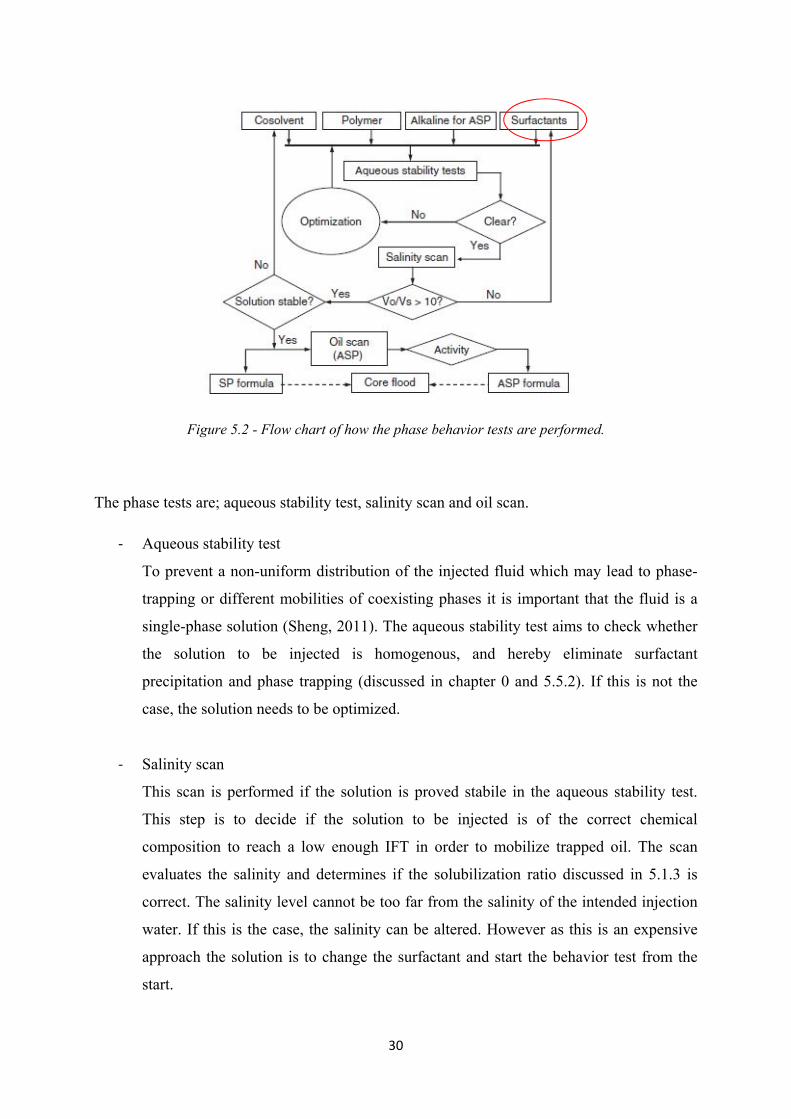
5.2.1 Phase behavior test
Prior to injection of the phase containing surfactants into the reservoir, the specific and
optimal chemical formula needs to be determined. This is the main objective of the phase
behavior tests. A flow chart is depicted in Figure 5.2.
30
Figure 5.2 - Flow chart of how the phase behavior tests are performed.
The phase tests are; aqueous stability test, salinity scan and oil scan.
- Aqueous stability test
To prevent a non-uniform distribution of the injected fluid which may lead to phase-
trapping or different mobilities of coexisting phases it is important that the fluid is a
single-phase solution (Sheng, 2011). The aqueous stability test aims to check whether
the solution to be injected is homogenous, and hereby eliminate surfactant
precipitation and phase trapping (discussed in chapter 0 and 5.5.2). If this is not the
case, the solution needs to be optimized.
- Salinity scan
This scan is performed if the solution is proved stabile in the aqueous stability test.
This step is to decide if the solution to be injected is of the correct chemical
composition to reach a low enough IFT in order to mobilize trapped oil. The scan
evaluates the salinity and determines if the solubilization ratio discussed in 5.1.3 is
correct. The salinity level cannot be too far from the salinity of the intended injection
water. If this is the case, the salinity can be altered. However as this is an expensive
approach the solution is to change the surfactant and start the behavior test from the
start.

31
- Oil scan
The oil scan is used if alkali, in addition to the surfactants, is added to the injection
phase. Alkalis have the same purpose as surfactants and may be added to make the
solution more economically feasible, as alkalis normally cost less.
5.2.2 Salinity
The salinity of the brine in the reservoir is an important factor. The salinity affects the
chemical composition of the surfactant, and may prevent it from influencing the IFT in a
beneficial way.
Before explaining how the salinity affects the system the term microemulsion needs to be
defined. A microemulsion is most easily described as a mixture of either surfactant and oil, or
surfactant and water or surfactant and both oil and water. It is a homogenoius phase which is
thermodynamicly stable (Sheng, 2011). Microemulsion is also described as micelle-solution if
the concentration of the surfactant is above the CMC. A micelle and the CMC were defined in
chapter 5.1.2.
When the level of salinity is low the surfactants will mix with the water and together they
form a microemulsion phase. At such a low salinity level the oil phase will be free of
surfactants. This is contrary to a high salinity level when the surfactants will mix with the oil
phase and form into a so called oil-external microemulsion. At this condition the water does
not contain any surfactants. At an intermediate salinity level the surfactants will form a
microemulsion with both the water and the oil. In addition there will be excess water and oil,
not containing any surfactants.
When the salinity level is low the microemulsion is called Type II(-), when the salinity level
is high Type II(+) and at an intermediate salinity level Type III (Sheng, 2011). Several studies
have been done on what characteristics the different types bring to a reservoir model, Table
5.1 sums up the advantages and disadvantages of the different types (Sheng, 2011). It can here
be noted that a modeled reservoir will be an ideal system and a real reservoir will to a larger
extent be far more complicated and not ideal.
The salinity level classified as the most desirable and advantageous is called the optimum
salinity level. Optimum salinity level is the average salinity in the salinity range covered by
Type III (Salanger, et al., 1979). At optimal salinity level the mixture of surfactant oil and

32
water or brine is near the so-called tricritical point where the phases become
indistinguishable, at this point the IFT will exhibit ultralow values as it approaches zero.
Hence, Type III is described as the preferred type of microemulsion (Green & G Paul, 1998).
The tension between the liquid phases can be difficult to measure at the desired ultralow
values. It has been shown that the IFT correlates with the solubilization ratio (defined in
chapter 5.1.3). The solubilization ratio is easier to measure than the IFT. When the
solubilization ratio is measured to be 10 or greater it is believed to be within the optimal
salinity range (Green & G Paul, 1998). As this is reached, the IFT can be measured and can be
expected to show ultralow values.
Eclipse only support and simulate for surfactants being in the water phase, thus phase II(-).
This is also somewhat desirable because by it limits microemulsions. The presence of
microemulsions indicates that the IFT is low enough for the capillary trapped oil to be
mobilized (Michaels, et al., 1996). Yet, it is not solely favorable because these
microemulsions contain a rather high concentration of surfactants. This concentration will be
delayed in the process of propagation. When it is desirable to keep the concentrations at a low
level the delay will be even more considerate. The presence of microemulsions may also
increase the viscosity of the oil which in turns may cause displacement instabilities. This
again will possibly require polymers to be added in the reservoir to stabilize the displacement
(Michaels, et al., 1996). This addition is expensive and desirable to avoid.
Table 5.1 - Shows the advantages and the disadvantages for the different types of microemulsions
(Sheng, 2011).
Type Advantages Disadvantages
II(-) Low phase trapping/adsorption Bypassing excess oil due to its high velocity
III Lowest IFT Phase trapping due to three-phase kr issues
II(+) Favorable kro Phase trapping due to its high viscosity
33
5.2.3 Temperature
In general the reservoirs in the North Sea are, including Norne, waterflooded and injection of
cold water will give temperature gradients (Skjæveland & Kleppe, 1992). A change in the
temperature will affect the solibilization ratio in the system, which in turns will shift the
optimum salinity level. It is therefore desirable to keep the system stable and avoid
unfavorable phase behavior due to temperature gradients. To obtain ultralow IFT if the
temperature increases the targeted salinity level will be expected to be higher as the
solubilization ratio decreases (Green & G Paul, 1998).
5.2.4 Oil composition
The type of oil in the reservoir will affect the relationship between oil and water and hence
how the surfactants will interact with the liquids. When the carbon number increase, the
optimal salinity will increase as well. Basically as the oil gets heavier the width of the salinity
region for Type III will expand and the solubility will decrease (Sheng, 2011). The oil in the
C-segment is light to intermediate and the width of the salinity region is not expected to
expand, which in turns leave the solubility unchanged.
5.3 Flooding of the reservoir
Through flooding of the reservoir the IFT will be lowered which in turns lowers the capillary
pressure and thus mobilizes the residual oil. This will increase the oil saturation and the oil
bank will be able to flow. Behind the oil bank the surfactant will prevent the oil from being
retrapped (Skjæveland & Kleppe, 1992). In order to achieve this in a successful way a
detailed plan where the correct strategy is denoted should be made. It may be necessary to add
a cosurfactant to the surfactant and it may also be necessary to add polymer to the chase
water. The reason for using a cosurfactant can be several. The surfactant chemicals are
expensive and may be thinned out, without losing their characteristics, by using a
cosurfactant. It can also be desirable to add a surfactant to avoid adsorption where that is
predicted. When adding polymers to the chase water the aim is to increase the viscosity of the
water phase to avoid fingering which leads to earlier breakthrough of the water, will be
mentioned in the next chapter. When the composition of the phase to be injected is decided
upon the strategy for flooding must be developed. This will be further discussed in chapter
6.6.

34
5.4 The effects of surfactants
As mentioned the main task for surfactants is to lower the interfacial tension in order to lower
the capillary pressure. This is the desired effect after flooding of the reservoir. By lowering
IFT and thus Pc the trapped residual oil will become mobile. The Laplace equation referred to
in chapter 2.1 shows the relationship between IFT and Pc:
= − = = ∆ (5.1)
Figure 5.3 - Illustrating the Pc equation (Skjæveland & Kleppe, 1992).
po in formula 5.1 and Figure 5.3 denotes pressure in the oil phase, pw denotes pressure in the
water phase, σ is the interfacial tension, θ the contact angle between the non-wetting (oil) and
wetting (water) phase, Δρ is the difference in density for the phases, r is the radius and H is
the height. Equation 5.1 is developed from the equation of static equilibrium on the interface
between oil and water in a cup containing a capillary tube (Lien, 2008). The capillary pressure
is the difference between the pressure of the non-wetting phase and the wetting phase (Lien,
2008). Figure 5.4 illustrates two pores/capillaries with different widths. Water is here the
wetting phase. As water is flowing through the pore space it will reach highest in the smaller
pore due to the smaller radius. The water will break through to production before the largest
pore is swept for all its oil. This is called snap-off and it is oil in this form that is called
residual oil saturation, Sor when the reservoir is water wet(Dr.Tran, 2006).
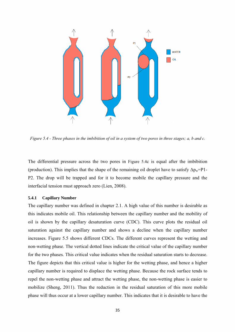
35
Figure 5.4 - Three phases in the imbibition of oil in a system of two pores in three stages; a, b and c.
The differential pressure across the two pores in Figure 5.4c is equal after the imbibition
(production). This implies that the shape of the remaining oil droplet have to satisfy Δpw=P1-
P2. The drop will be trapped and for it to become mobile the capillary pressure and the
interfacial tension must approach zero (Lien, 2008).
5.4.1 Capillary Number
The capillary number was defined in chapter 2.1. A high value of this number is desirable as
this indicates mobile oil. This relationship between the capillary number and the mobility of
oil is shown by the capillary desaturation curve (CDC). This curve plots the residual oil
saturation against the capillary number and shows a decline when the capillary number
increases. Figure 5.5 shows different CDCs. The different curves represent the wetting and
non-wetting phase. The vertical dotted lines indicate the critical value of the capillary number
for the two phases. This critical value indicates when the residual saturation starts to decrease.
The figure depicts that this critical value is higher for the wetting phase, and hence a higher
capillary number is required to displace the wetting phase. Because the rock surface tends to
repel the non-wetting phase and attract the wetting phase, the non-wetting phase is easier to
mobilize (Sheng, 2011). Thus the reduction in the residual saturation of this more mobile
phase will thus occur at a lower capillary number. This indicates that it is desirable to have the

36
reservoir water wet. The wettability is further discussed in the next chapter. The normal range
for the value of the capillary number is in the range of 10-7 to 10-5, and needs a considerable
increase to reduce the residual saturation.
Figure 5.5 - Capillary Desaturation Curve (CDC) (Skjæveland & Kleppe, 1992).

37
5.4.2 Wettability
The wettability is defined as the preference of a solid to be in contact with one fluid rather
than another (Dr.Tran, 2006). The wettability of Norne C-segment is mixed-wet (Verlo,
2008). This indicates an inhomogeneous and thus not strongly water-wet nor strongly oil-wet.
Figure 5.6 depicts this.
Figure 5.6 - Wettability (Abdallah, et al., 2007).
The wettability affects the amount of residual oil that can be produced. The residual oil
previously introduced as capillary trapped, is the oil droplets inside the pores of a water-wet
reservoir. In an oil-wet reservoir the residual oil is positioned along the “walls” in the pores.
The amount of residual oil a reservoir of this wetting will, due to no capillary trapping, be less
than for a water-wet reservoir. The oil migrates out from the pores and, and the recovery can
in theory be 100%. In Norne, where the wetting is mixed-wet, both of the conditions above
are found. The use of surfactants are foremost a technique tested for water-wet reservoirs
(Abdallah, et al., 2007). The distribution and flow of fluids in pores is therefore to a large
extent affected by the wettability of the porous medium (Awan, et al., 2006). It has been
suggested (mentioned in chapter 2.1) to instead of adding surfactants to lower the IFT and
hence the capillary pressure, the surfactants should aim to change the wettability in the
reservoir (Rao, et al., 2006). This requires less surfactant and can then prove to be less
expensive. Thus mentioned, this is not a subject in this report.

38
5.4.3 Relative permeability
When flooding the reservoir with water containing surfactants, the relative permeability will
be affected. The relative permeability is defined as one fluids ability to flow in the presence of
another fluid (Dr.Tran, 2006). When the oil saturation is decreasing the relative permeability
to water will increase. When looking at the water mobility and the mobility ratio (formula
2.4) defined in chapter 2.1 these values will increase when the water relative permeability
increases. It is not desirable for the mobility ratio to increase too much as this may lead to an
earlier breakthrough of the water phase. To reduce the mobility of the injected water that is
chasing the surfactant solution it might be necessary to add a cosolvent (polymer) to it.
5.5 Challenges
The theory of how the surfactants target to extract more oil is simple. The implementation
however, is not as easy. There are challenges that need to be taken into consideration in order
to successfully implement surfactant flooding of a reservoir. Firstly the measurement of the
effective IFT in a porous media is difficult. This difficulty limits the laboratory modeling and
prediction of surfactant flood performance (Zhang, et al., 2007). When measuring the IFT in
the laboratory the conditions will be ideal. The conditions in-situ in the reservoir is far from
ideal.
When the surfactant phase is injected into the reservoir occurrences like precipitation,
adsorption and phase trapping of the surfactant will happen. All these processes lead to
retention of surfactants which in turns potentially raise the effective IFT in the reservoir from
the value measured beforehand in laboratory, and thus contribute to oil trapping (Zhang, et al.,
2007), (Green & G Paul, 1998). It has also been suggested that nearly 90% of the injected
surfactants are retarded by the formation when passing through the reservoir (Skjæveland &
Kleppe, 1992). If this suggestion is correct, only a small portion of the surfactant actually
contributes in lowering the IFT. Due to this it is very important to calculate the amount of
surfactants actually needed in order to successfully implement the flooding. There are also
major challenges when it comes to economic feasibility of projects regarding surfactant
flooding. As for the Norne field the offshore location will also represent a challenge. The
stated challenges are discussed next.

39
5.5.1 Adsorption
Adsorption is when the surfactant adheres or sticks to the surface of the reservoir. As Figure
5.7 depicts it is the charged head group that will attach to the surface which is oppositely
charged. This is the major cause for surfactant retention and thus loss of surfactant.
Adsorption can be lowered by adding alkaline as a cosurfactant (Dang, et al., 2011). The
adsorption of the surfactants is a complicated matter, but can be generalized into four different
stages or regions depending on the concentration of surfactants. When the concentration is
low, the adsorption will be increasing linearly as the amount of chemicals increase. This is the
first region shown in Figure 5.8. In the second region the increase in surfactant concentration
will lead to a rapid increase in the adsorption. In the third region the adsorption subsides as
the concentration is reaching the critical micelle concentration (CMC). When this
concentration is reached, in region four, the adsorption will stay at a constant level
(Skjæveland & Kleppe, 1992).
Figure 5.7 - Illustrating how the head groups cling to the surface in the phenomena of adsorption
(Dang, et al., 2011).

40
Figure 5.8 - Adsorption curve (Skjæveland & Kleppe, 1992).
5.5.2 Precipitation
A precipitate is a by-product followed by a chemical reaction (Schlumberger, 2011). These
by-products can be a result of phase separation of surfactants and a potential cosurfactant or
separation of the different kinds of surfactants in solution (Green & G Paul, 1998). This may
be a result of a failed aqueous stability test. A preflush of the reservoir, which is injecting
water into the reservoir prior to the surfactant phase, can reduce or prevent precipitation
(Schlumberger, 2011). Using Alcohol as a cosurfactant has also proved to be beneficial for
reducing precipitation (Dang, et al., 2011). It has also been proposed to increase the
concentration of surfactants above the CMC because precipitates will not form once micelles
have started to form (Sheng, 2011).

41
5.5.3 Economy
A surfactant flooding project does require a large and spacious economy. The high front-end
investments combined with delayed production also require that the oil price is above some
threshold price (Tomich, et al., 1987). The front-end investments are the chemicals and the
equipment to be used. In some projects it may be of interest to add a cosurfactant or
cosolvent as previously mentioned to reduce the cost. For the projects where the chase water
following the surfactant slug contains polymers, expenses for this are added. This will not be
explained further here, however it can be noted that it is costly. As for the Norne field extra
economic constrains will apply because of the offshore location. This is explained next. Prices
and costs are further explained in chapter 0.
5.5.4 Field location
To plan and execute a surfactant flooding project for a reservoir located offshore, such as the
Norne field is challenging. Firstly the space to store the chemicals to be injected is limited.
This is problematic when large quantities are to be injected daily injection. As an example
injecting 3000m3/day of a 2% surfactant solution will require the handling of 60tons of
chemicals a day (Skjæveland & Kleppe, 1992). The plan for using chemical flooding must be
developed early in order to handle the need for such a storage demand. This will put
constrains on the financial planning and economic feasibility. In addition to the issues
regarding storage, the surfactants need to be transported offshore. This makes offshore
projects extra challenging compared to onshore ones regarding economy and logistics.
5.6 Selection of surfactant
The selection of surfactants is a challenging task. Chapter 5.2 presented the term phase
behavior which is important to be aware of. The chemical reactions the surfactant slug
undergoes in the reservoir can to some extent be predicted and needs to be fully understood in
order to select the best alternative. In general the reservoir engineer is not involved in
deciding the chemical composition of the surfactant used, as this is the work of a chemist. The
chemical is as previously mentioned commonly an anionic surfactant.

42

43
6 Reservoir simulation
The simulations presented in this report aim to boost the recovery from the Norne C-segment
by injecting surfactants. The desired outcome is to achieve as high and satisfactory value of
incremental oil recovery possible. An economical evaluation to decide on the feasibility of
such a project is performed by calculating the Net Present Value (NPV).
6.1 Eclipse 100
Eclipse 100 is a black oil simulator. The data file to be simulated by Eclipse is constructed in
a special way. This particular structure is explained in Appendix C. Among several features
Eclipse provides modeling options to handle surfactant flooding.
6.2 The surfactant model
The surfactant model does not aim to model the detailed chemistry of a surfactant process, but
rather to model the important features of a surfactant flood on a full field basis. The surfactant
is assumed to exist only in the water phase and the distribution of injected surfactant is
modeled by solving a conservation equation for surfactants within this phase. At the end of
each time-step, after the oil-, water- and gas- flows have been calculated, the concentration of
the remaining surfactants are updated using fully-implicit calculations (Schlumberger, 2011).
This implies that Eclipse does not model the phase behavior of the surfactants. It only models
the effect surfactants have on relative permeability assuming that it is in the water phase. This
is done by introducing interfacial tension as a function of the surfactant concentration to the
model. The capillary number will be calculated as a function of the interfacial tension and
further an interpolation constant is given as a function of the capillary number. Eclipse then
interpolates between the relative permeability values for the solution not containing
surfactants and the solution which does contain surfactants. Together with the capillary
desaturation curves and the low tension relative permeability curves, the chemical adsorption
is given as input. The keywords required to initiate and use the surfactant model are explained
in Appendix E, and how Eclipse calculates is explained in Appendix D.
6.3 Input values used in the surfactant model
The values used in the surfactant input file are collected from Yugal Kishore Maheshwari’s
master thesis and are originally provided by Statoil ASA. As previously mentioned the type of
surfactant used is generally not an issue to the reservoir engineer. A reduced version showing
key data is enclosed in Appendix F. In order to successfully implement the surfactant model

44
some of the keyword needs to be defined for each of the PVT regions or for each of the
saturation tables in the model. These numbers are 2 and 107 respectively.
There are five different tables in the surfactant input file. Among these the surfactant viscosity
table, the capillary desaturation curve and the adsorption table are the most influential. By
changing these impact will be notable.
The critical capillary number in the surfactant dataset is 10-5, this is the highest value for
immiscible conditions. Exceeding this value indicates miscible conditions and thus higher
surfactant concentrations. The residual oil saturation is as mentioned in chapter 5.4.1 reduced
when the critical capillary number is reached.
Prior to adding the surfactants the IFT is 3*10-2N/m. The presence of surfactants lowers the
value with a factor of 10-4 to 10-6N/m. This is in accordance with the ultralow values for IFT
described in literature (Sheng, 2011).
The value of adsorption given in the input file is kept constant. The value is 0,17mg
surfactant/g of rock. The average adsorption value for reservoir rocks in the North Sea is
reported by literature to be around 0,4mg/g (Jakobsen & Hovland, 1994).
The viscosity of the surfactant solution is given as a function of the surfactant concentration.
When the surfactant concentration is zero, the input viscosity is equal to water. As the
surfactant concentration increases the solution viscosity increase. A high viscosity of the
surfactant solution, or the displacing phase, will seek to lower the mobility ratio between the
displacing and displaced phase. This will lead to a more stable displacement.

45
6.4 Economic model
The economical evaluation performed in this report is of a very simple nature. The revenue
for each year is discounted back to a present value. The total revenue of the whole surfactant
flooding project from 2007 to its end in 2022 is the sum of the present values for each year.
The revenue for each year is simply the injected surfactant times the surfactant price
subtracted from the oil production times the oil price. Despite the fact that important factors
regarding CAPEX and OPEX are left out, it provides a good indication of a projects potential.
It is a simple NPV calculation which gives an indication whether a project is feasible or not,
and is given by the formula (Drake & Fabozzi, 2009):
= ∑ ( ) (6.1)
N is the total number of discounting periods or time intervals, t is the current time, Ct is the
revenue at the given time t and i is the discount rate.
A discount rate of 8% is used. The oil price has varied from US$100 to US$88 per barrel the
last five years (Bloomberg, 2012). A value of US$110/bbl is used in the calculations. The
costs associated with the injections of surfactants both include the cost of the chemical itself,
and logistics such as transport. The price could typically be 7US$/kg, where the isolated cost
for the surfactant is between US$1 and US$2 per kg (Sandengen, 2012). The cost of
surfactants in this report excludes logistic additives. 100US$/bbl oil and 1US$/kg surfactant
was used in the calculations
6.5 Procedure for simulation
Different cases were tested in order to develop an optimum injection strategy. A large variety
of different scenarios can be tested and investigated in order to maximize the recovery. This
report is as previously mentioned an extension of the report “Introduction to surfactant
flooding for EOR on the Norne Field, C-segment”, the cases tested in this report is therefore
based on scenarios presented in that project. Purely water injection will be used as base case
and as a comparative case to the surfactant cases.
The historical data for the Norne C-segment is available through year 2006. Accordingly, the
reservoir performance from 2007 until 2022 is purely a prediction. Water is injected in the
beginning of 2007, and constantly through the expected life time. With water as the only drive
mechanism a recovery of approximately 49%, on a field basis, is calculated by Eclipse. As

46
additional wells, from other segments than the C-segment, are included in this estimate due to
the pressure support it is probably a bit lower. Nevertheless 49% is a fairly good estimate
which the injection of surfactants aims to raise.
In 2007 there are 5 production wells operating. These are B-2H, D-2H, D-1CH, B-4DH and
K-3H. They are all perforated between layers 5 through 10, which is in the Ile formation. The
four water injectors; C-1H, C-2H and C-4H are in 2007 perforated between layers 14 through
20, which is in the Tofte formation.
6.6 Simulation Cases
Base case
The base case is the case of water flooding for maintaining a pressure high enough to recover
oil. This is used as a comparative case to the cases where surfactants are injected. All the three
injection wells are used in the base case and they are perforated in the target layers which for
most of the cases are layer 5 through 12.
Case 1 – Formation selection
80% of the oil is said to be situated in the Ile and Tofte formation. These areas are therefore
characterized as target areas for the surfactant flooding. However, it is of interest to decrease
the area of interest to decrease the amount of chemicals needed and in the simulation aspect,
to better see the effect. To do so, injection into Ile and Tofte is compared with respect to oil
recovery. Injection well C-2H is used and is in the first scenario perforated in layer 5-11,
which is in Ile, and in 12-18 in the second scenario, which is in Tofte. The cumulative oil
production is compared to water injection in the same layers.
Case 2 – Well selection
The C-segment is a relatively large reservoir. The injectors are situated in each corner (Figure
4.5 depicts this). Adsorption and loss of chemicals can, as previously described, be an issue in
surfactant flooding. The evaluation and decision of what well to use is therefore important.
Case 2 is an extreme case testing continuous injection of surfactants in each of the wells
separately, and combined using all wells. The wells are perforated in the Ile formation.
Case 3 – Surfactant concentration
In accordance with literature the adsorption of surfactants will stagnate as the surfactant
concentration increases (Skjæveland & Kleppe, 1992). When the critical micelle
concentration is reached, the adsorption becomes constant and the reservoir rock is fully

47
saturated with surfactant. Figure 5.8 in chapter 5.5.1 depicts this relationship. In this case the
concentration of surfactants in the injected phase will be altered to see the impact on oil
recovery. As a comparison to the value of 10 kg/Sm3 used in case 1, values of 5 kg/Sm3 and
30 kg/Sm3 are simulated for.
Case 4 – Slug size
This case evaluates the use of a surfactant slug, rather than continuous injection. Scenarios
using a slug size of 2, 5 and 8 years will be simulated. Well C-2H is used as injection well, it
is perforated in the Ile formation and the surfactant concentration is 10 kg/Sm3 in case 4a and
5kg/Sm3 in case 4b.

48

49
7 Results from the simulation Appendix J and Appendix K shows the production, NPV and adsorption values in their entirety. The plots in the next chapters are based on this.
7.1 Case 1 – Formation selection
Figure 7.1 depicts the incremental cumulative oil production when injecting into the Ile
formation versus the Tofte formation. The injection of surfactants was using one well, using a
two year slug and injecting from 2007 until 2009.
Figure 7.1 - Incremental Cumulative Oil production for Case 1.
The case of injecting surfactants in Ile results in a recovery approximately 1% higher than
injecting the same amount of surfactants in Tofte. When both the producers and injectors are
perforated in Ile the oil production rapidly increases as the surfactants are added. Around
2013 it reaches its top production and experience a slight decline towards year 2022.
When injecting surfactants into Tofte the production is not increased until after 2012. The
production is even lower than basecase before increasing to the same level as the previous
scenario. The gap between the two curves is relatively large until the end of the evaluated
period. This implies that injecting in Ile will result in money earned at an earlier stage than if
injection in Tofte. As mentioned economy is important and can make or break such a project.
-5,00E+04
0,00E+00
5,00E+04
1,00E+05
1,50E+05
2,00E+05
2,50E+05
2007
2008
2009
2010
2011
2012
2013
2014
2015
2016
2017
2018
2019
2020
2021
2022
Incr
emen
tal O
il Pr
oduc
tion
Sm3
Year
Case 1: Incremental Cumulative Oil Production (Sm3)Injection into ILE Injection into TOFTE

50
Figure 7.2 depicts the adsorption in the two scenarios. It shows that the adsorption is highest
when injection in Tofte. For injecting a two year slug, the adsorption is 31% for Ile and 34%
for Tofte. In the following cases the surfactants is injected in Ile.
Figure 7.2 - Total adsorption of surfactants in Case 1.
7.2 Case 2 – Well selection
Figure 7.3 shows the incremental oil recovery from each of the wells. The concentration of
surfactants used in this case is 10 kg/Sm3 and the injection is continuous.
Injecting surfactants through all of the three injectors seek to the highest recovery of oil with
an 1,23% increase in oil production. When evaluating each well separately using well C-2H
gave the best result with an increase in production of 0,94%. The injector C-3H showed the
poorest result with an 0,08% incremental recovery. Table 7.1 provides an overview of the key
values. Figure 7.4 depicts how the chemicals spread after injection. Blue color represents high
concentration and pink color represents zero concentration. The white arrow indicates the
position of the injector. The pictures to the left depict the situation in 2009, two years after
injection, whilst the pictures to the right depicts the situation in year 2017, 10 years after
injection start. The white spots in the figures to the right illustrate the position of the
producers.
0,00E+00
5,00E+06
1,00E+07
1,50E+07
2,00E+07
2,50E+07
3,00E+07
2007
2008
2009
2010
2011
2012
2013
2014
2015
2016
2017
2018
2019
2020
2021
2022
Adso
rptio
n (k
g)
Year
Case 1: AdsorptionILE TOFTE

51
In general the adsorption is low for all the cases, with values below 40%. As for production of
surfactants, well C-3H has the highest value when evaluating the single well scenarios.
Table 7.1 - Total oil production, increase in total production, NPV and adsorption for Case 2.
Figure 7.3 - Incremental Cumulative Oil production for Case 2.
Case 2Surf price (US$/Sm3) 1 OPT Increase NPV AdsorptionOil price (US$/bbl) 100 Sm3 % Mill US$ %Basecase 4,81E+07 - - -C-1H 4,85E+07 0,82 -219,81 20,2C-2H 4,86E+07 0,94 -150,83 12,3C-3H 4,81E+07 0,08 -320,28 12,2All Wells 4,87E+07 1,23 -750,58 12,5
-2,00E+05
-1,00E+05
0,00E+00
1,00E+05
2,00E+05
3,00E+05
4,00E+05
5,00E+05
6,00E+05
7,00E+05
2006
2007
2008
2009
2010
2011
2012
2013
2014
2015
2016
2017
2018
2019
2020
2021
2022
Incr
emen
tal O
il Pr
oduc
tion
Sm3
Year
Case 2: Incremental Cumulative Oil Production (Sm3)
C-1H C-2H C-3H All Wells

52
C-1H
C-2H
C-3H
2009 2017
Figure 7.4 - Propagation of surfactants.

53
7.3 Case 3 – Surfactant concentration
A surfactant concentration of 10 kg/Sm3 has previously been used. In this case both a lower
and a higher concentration, of 5 kg/Sm3 and 30 kg/Sm3, are compared to the previously used
concentration. The injection is continuous and the surfactants are injected through well C-2H.
The total increase in oil production is 0,60%, using a low concentrated surfactant solution in
the reservoir model. Figure 7.5 shows that the increase is highest and most rapid from 2009
through 2014, after this it stagnates and has a slower increase.
A surfactant concentration of 10kg/Sm3 follow the trend of the low concentrated injection
phase, thus it increases to a higher level before it slows down in the last half of the production
period. The increase in oil production is 0,94%.
Using 30 kg/Sm3 provides a higher oil production than the two previous scenarios, which
results in a steeper slope in Figure 7.5. The trend is more or less the same as for low and
intermediate concentrations as the rate of increase stagnate to a more linear level around 2014.
The total increase in oil production is 1,49%. Using a highly concentrated injection also had
the lowest value of adsorption.
The NPV values for the three scenarios are negative even with an oil price considered
relatively high. Table 7.2 depicts the incremental cumulative oil production at the end of
production ant the total NPV. (An extended version of this table is found in Appendix J.)
Table 7.2 - Total oil production, increase in total production, NPV and adsorption for Case 3.
Case 3Surf price (US$/Sm3) 1 OPT Increase NPV AdsorptionOil price (US$/bbl) 100 Sm3 % Mill US$ %Basecase 4,81E+07 - - -Surf. concentration = 5 kg/Sm3 4,84E+07 0,60 -33,18 24,7Surf. concentration = 10 kg/Sm3 4,86E+07 0,94 -150,83 14,7Surf.concentration = 30 kg/Sm3 4,88E+07 1,49 -724,22 6,1

54
Figure 7.5 - Incremental Cumulative Oil production for Case3.
7.4 Case 4 – Slug size
The injection has been continuous in the previous cases. The duration of the injection is
altered in this case. Concentrations of 5 kg/Sm3 and 10 kg/Sm3 are used in case 4a and 4b,
respectively.
The incremental oil is highest for injecting an 8 year slug, this gives an increase in recovery of
0,51%. However it is followed closely by the 5 year slug with a recovery of 0,49%. Injecting
with a two year slug increase the production by 0,44%. All the tree scenarios have the same
trend the first five years. In 2012 the oil production in the scenario with the shortest slug
declines moderately towards the end in 2022. The two other scenarios continue to increase
until 2022. The incremental production for the longest slug has lower slope than when using
the intermediate slug. The adsorption is highest at approximately 55% when injecting for 8
years. Figure 7.6 depicts the behavior. Table 7.3 sums up the key data recovered and show that
none of the scenarios lead to a positive net present value.
-1,00E+05
0,00E+00
1,00E+05
2,00E+05
3,00E+05
4,00E+05
5,00E+05
6,00E+05
7,00E+05
8,00E+05
2007
2008
2009
2010
2011
2012
2013
2014
2015
2016
2017
2018
2019
2020
2021
2022Incr
emen
tal C
umul
ativ
e O
il Pr
oduc
tion
Sm3
Year
Case 3: Incremental Cumulative Oil Production (Sm3)
Surf. concentration = 5 kg/Sm3 Surf. concentration = 10 kg/Sm3 Surf. concentration = 30 kg/Sm3

55
Table 7.3 - Total oil production, increase in total production, NPV and adsorption for Case 4a.
Figure 7.6 - Incremental Cumulative Oil production for Case 4a.
Case 4b is, besides halving the surfactant concentration to 5 kg/Sm3, identical with 4a. The
results are shown in Figure 7.7 and follow the same trend to some extent. Only the incremental
production from the 8 year slug deviates from the two other scenarios. It returns a production
on a continuously higher level than the shorter slugs. Despite this, the scenario using the
shortest slug is the only one leading to a positive net present value. The adsorption is quite
similar for all of the three scenarios in the case. Table 7.4 below summarizes this.
Case 4a, 10 kg/Sm3
Surf price (US$/Sm3) 1 OPT Increase NPV AdsorptionOil price (US$/bbl) 100 Sm3 % Mill US$ %Basecase 4,81E+07 - - -Slug size = 2 years 4,83E+07 0,22 -17,89 31,4Slug size = 5 years 4,83E+07 0,49 -57,43 35,1Slug size = 8 years 4,84E+07 0,51 -120,15 54,8
-5,00E+04
0,00E+00
5,00E+04
1,00E+05
1,50E+05
2,00E+05
2,50E+05
3,00E+05
2007
2008
2009
2010
2011
2012
2013
2014
2015
2016
2017
2018
2019
2020
2021
2022
Incr
emen
tal O
il Pr
oduc
tion
Sm3
Year
Case 4a: Incremental Cumulative Oil Production (Sm3)
Slug size = 2 years Slug size = 5 years Slug size = 8 years

56
Table 7.4 - Total oil production, increase in total production, NPV and adsorption for Case 4b.
Figure 7.7 - Incremental Cumulative Oil production for Case 4b.
Case 4b, 5 kg/Sm3
Surf price (US$/Sm3) 1 OPT Increase NPV AdsorptionOil price (US$/bbl) 100 Sm3 % Mill US$ %
4,81E+07 - - -4,83E+07 0,33 5,02 33,34,83E+07 0,37 -21,36 34,24,83E+07 0,40 -43,43 30,2
BasecaseSlug size = 2 yearsSlug size = 5 yearsSlug size = 8 years
-5,00E+04
0,00E+00
5,00E+04
1,00E+05
1,50E+05
2,00E+05
2,50E+05
2007
2008
2009
2010
2011
2012
2013
2014
2015
2016
2017
2018
2019
2020
2021
2022In
crem
enta
l Cum
ulat
ive
Oil
Prod
uctio
n (S
m3 )
Year
Case 4b: Incremental Cumulative Oil Production (Sm3)
Slug size = 2 years Slug size = 5 years Slug size = 8 years

57
8 Analyses and Discussion
Case 1 – Formation selection
As previously mentioned the water injectors were perforated in the Tofte formation in the
original version of the reservoir model. When evaluating the oil in place in Ile and Tofte in
2007 the values are 31% and 21% respectively.
When using water injection it is beneficial to keep the injection below the producer to sweep
the reservoir updip. This is to benefit from gravitation as the water is heavier then oil and will
sink below the oil phase. When adding surfactants to the displacing phase other factors must
be taken account for. With large spacing between injector and producer there will be an
increasing likelihood and risk for adsorption. And if the surfactants have to travel long
distances to reach the target area, the amount of chemicals needed is increased.
When reviewing the results, the difference in recovery between injecting into Ile and into
Tofte is very little. This is somewhat surprising. Due to large spacing between injector and
producers, in the case of injection in Tofte, the amount of adsorption was expected to be
higher. However the adsorption is only 34% when injecting into Tofte and 31% when
injecting into Ile. This is a relative low value as the adsorption can be expected to reach levels
of 90% (Skjæveland & Kleppe, 1992). Even though the cumulative results of the two
scenarios are of the same order in 2022, the trend differs from each other. As mentioned in the
results is the incremental oil production for injection in Ile increasing rapidly at the beginning
before decreasing after its peak in 2014. When injecting surfactants in Tofte the incremental
production decreases slightly in the beginning before rising constantly. One may question if a
longer production period would benefit the scenario of injection into Tofte because of its
rising trend.
Because higher incremental production is the ultimate aim of this report, injecting into Ile was
chosen as the main strategy for the further analysis. As the difference between the two
scenarios was sparse it would have been interesting to use both formations, however only one
was chosen.

58
Case 2 – Well selection
The expectations for case 2 were to some extent met. Using all the wells for injection of
surfactants returned an oil production consistently higher than basecase and thus the highest
incremental oil recovery.
The injector C-1H is situated in between three faults. These faults obstruct propagation of
surfactants to a certain degree (depicted in Figure 7.4). In addition to this the producers
situated closest to C-1H are shut in after 2007. This results in a longer way for the surfactants
to travel. Due to this the amount of adsorbed surfactant is highest when using C-1H. Yet, as
mentioned in the results, the volumes of adsorbed chemicals were uncritical for all scenarios
in the case.
Injecting through well C-2H leads to a good distribution of surfactants. This provides a good
sweep, and the effect is immediate. Oil production is rapidly increased at an early stage
compared to the scenarios using the other wells. This is a clear advantage when evaluating the
economical aspect. The investments associated with a surfactant flooding project are major
especially at the beginning; a lot due to facilitation. Income to cover these expenses will be
crucial for a project.
The scenario using well C-3H showed a somewhat unexpected result when the continuous
injection of surfactants resulted in poorer recovery than the basecase for majority of the time.
This was unexpected because C-3H is the injection well situated closest to the producers,
which should limit the exposure to retention of surfactants. Yet, it results in too early
production of surfactant solution which obstructs oil from being produced.
The collective review of case 2 showed a far poorer result than anticipated. The injection was
continuous, which should secure a good sweep. Despite this, breakthrough and production of
the injected solution will start before the low permeable layers are reached. This is because
the injected fluid will spread through high permeability zones first and the low permeable
layer may remain untouched due to this (Green & G Paul, 1998). In addition to this, the wells
have water breakthrough. This will make it easier for the injected fluid to follow the
developed path instead of penetrating new areas.
Due to the cost of chemicals and facilitation of such a project injection on a continuous basis
is not feasible (Dang, et al., 2011). All the scenarios in case 2 resulted in negative NPV’s.
59
Case 3 – Surfactant concentration
To make the project feasible, using a low concentration of surfactants is suggested in
literature (Skjæveland & Kleppe, 1992). This is among other things to make the supply and
handling of chemicals easier, which especially applies for offshore projects. Yet, the
concentration should be kept high enough to not obstruct the solubility between the oil and the
injected water solution. It is desirable to have the concentration of surfactants at a level so that
the CMC, explained in chapter 5.1.2, is reached. At this level more oil can be solubilized.
The simulation results with varying concentration showed that the highest concentration
recovered the most oil. This was expected as high concentration both decrease the IFT to the
lowest level and increase the solution viscosity to the highest level. Lower IFT lead to lower
capillary force and thus higher amount of residual oil mobilized. The increased solution
viscosity will benefit the mobility ratio (M) explained in chapter 2.1. A higher viscosity of the
displacing phase will lower M, which in turns stabilizes the displacement. In addition to this
the adsorption was as low as 6%. It is suggested that a highly concentrated slug is more stable
and may be less exposed for adsorption (Skjæveland & Kleppe, 1992). The combination of
these factors increase the production by 1,49%.
When decreasing the concentration to a third, using 10kg/Sm3 the oil production is increased
by 0,94%. This implies that cutting the amount of surfactants needed to a third only decrease
the enhanced oil production by 0,55% compared to the highly concentrated injection. As for
the even lower concentration of 5kg/Sm3, the total oil production is increased to 0,60% which
is 0,90% lower than the highly concentrated injection. In spite of the highest recovery, the
difference between in incremental oil recovered in the scenarios is low and fairly
insignificant. The additional increment is not enough to justify the higher surfactant
requirement.
Case 4 – Slug size
A continuous injection of surfactants can, as previously mentioned, never be feasible. The
injection of surfactants as a slug returns only around half the amount of incremental oil as
continuous injection. The most likely reason for this is adsorption and loss of chemicals.
Injecting a large slug with low concentration is described as attractive (Skjæveland & Kleppe,
1992). However, the only scenario providing a positive NPV value was injecting a low
concentrated slug in the shortest period tested (2 years). The revenue was low, but the only
valuable project. According to Harwell, Schetner and Wade at University of Texas an optimal

60
injection strategy for minimizing surfactant losses does exist. Yet it depends on the nature of
surfactant mixture used in the flood, and can be difficult to detect. This report only use a
single surfactant when injecting and hence finding the optimum injection strategy should be
possible. In order to know if the optimum injection strategy of the three scenarios tested here
is ideal, it must be compared to several scenarios.
Validation of data and the reservoir model
Reservoir simulation on a full field model requires a lot of input data to estimate desired
properties. When working with such a large model as Norne, which has been modified by
numerous of involved parties, the validation of data may be questioned. The surfactant input
file used is as previously mentioned, collected from another master thesis regarding the Norne
field and its E-segment. It is originally provided by Nan Cheng and Statoil ASA
(Maheshwari, 2011). The way the IFT was defined in the original dataset was questionable.
The IFT increased for the two highest values of the concentration. This provided a decrease of
the IFT by a factor of 10-4 before an increase which designated the IFT at the highest
concentration to only be lowered by a factor of 10-2. This does not correspond with literature
where a reduction of IFT by a factor of 10-4 is indicated as desirable for the North Sea
(Hovland and Jakobsen). As this was detected in time, the input datafile was altered to make
the IFT decrease with increasing concentration. However, this may indicate that other
undetected errors exist.
One may also discuss if this set of data is compatible with the reservoir and fluid properties
defined for the Norne C-segment. When simulating, the output file contained on an average
200 problems and 70 warnings. These were in most cases related to convergence failure, and
did not abort the simulations. Due to this they were overlooked.
In addition to this, the history matching performed prior to the simulations may possible have
been imprecise. This may have led to an uncertain prediction of the reservoir performance
from 2007 to 2022.

61
General
If the volume of incremental oil solely is the focal point of discussion, the optimal case after
evaluation is to continuously inject using a surfactant concentration of 30 kg/Sm3 via C-2H.
However, as previously enlightened continuously injecting is not realistic as both the costs
and handling will prevent it. When designating the NPV value as the determining factor the
case with injecting a low concentrated slug for two years was the optimum scenario. This case
increased the recovery by 0,16%. In comparison the case with continuous injection raised the
oil production by 1,49%.
These recoveries are surprisingly low. The incremental oil recovery will vary from field to
field. However, using just surfactants as the active chemical can be expected to return a
recovery efficiency of about 5-7% (Lakatos, et al., 2007). These percentages are from realistic
cases, and not continuous injection. When assessing these results to the results obtained from
the C-segment the success of using surfactants here is questioned. As surfactant flooding was
elected as the best EOR method to be used at the C-segment one would seemingly expect a
higher increase in oil production.
The surfactants target to lower the IFT which in turn lowers the capillary pressure and the
residual oil will be mobilized. The low recovery may indicate that one or more of these steps
not are fulfilled. A possible reason to this can be that the oil being produced from the
reservoir not is capillary trapped. As water injection nearly is as successful, a displacement
based on mobility difference between the phases seems to be enough. The reason for this can
potentially be that the injection of surfactants is too early, or that the capillary trapping is too
low.
A factor which may have an impact on the situation is the wettability. The amount of capillary
trapped Sor is, as previously mentioned, by far largest in a strongly water-wet reservoir. The
wettability in Norne was in chapter 0 described as inhomogeneous and thus mixed-wet. If the
larger portions of the reservoir are oil-wet, thus not strongly, the residual oil is not capillary
trapped. This will imply that the injected solution will bypass the oil without significantly
increasing the oil production. Considering that there are large areas where the oil is the
wetting phase, this might obstruct the oil production. This is due to that the rock tends to
attract the wetting phase (Sheng, 2011).
Another factor interesting to discuss is the fact that Eclipse overlooks the importance of phase
behavior. The simulation will be a simplification of the real and complex situation. This is

62
always the case with reservoir modeling and simulation. However phase behavior is quite
important and might affect the result. A simulation program developed by the University of
Texas called UTCHEM, take phase behavior into account when simulating. Before deciding
upon if a surfactant flooding project should be implemented an analysis using such a
simulation program tool should perhaps have been executed. For the C-segment at Norne the
recovery was probably too low to expect a result making it feasible to plan surfactant flooding
as a method for enhancing the recovery.

63
9 Conclusion
The demand for hydrocarbons are constantly growing, however the resources are limited. This
implies that EOR will be important to maintain oil production. Surfactant flooding is one such
method. By lowering the IFT between oil and water the surfactants mobilize the residual oil.
Through the process of screening, surfactant flooding was designated as an EOR method
suitable for the C-segment at Norne.
The reservoir model was prepared for simulation in Eclipse through history matching. Due to
the lack of history data regarding the pressure, the alterations were made adjusting vertical
barriers. However, to group the correct wells in the C-segment provided a better match.
The surfactant flooding of the reservoir returned a surprisingly low result. The following sums
up the important factors:
- Using injection well C-2H recovers the most incremental oil.
- The recovery was lower than anticipated. The largest increase in oil recovery is
1,49%. This result was obtained with continuous injection through well C-2H using a
high concentration (30kg/Sm3) of surfactants.
- Adsorption of surfactants was relative low, suggesting that the low recovery not is due
to loss of chemicals to the formations.
- High costs of surfactants make the profitability of such a project difficult.
- Only one of the 10 scenarios returned a positive NPV. This was using a low surfactant
concentration for a period of two years. However the income was low and the
incremental oil recovery was only 0,16%..
- The NPV strongly depends on oil price and surfactant price.
- As the aim of increasing the oil recovery through surfactant flooding is not satisfied
and thus it is not a recommended EOR method for Norne C-segment.

64

65
10 Uncertainties
In a reservoir simulation project there are a large amount of uncertainties. These spans from
the data the reservoir model is based on, the different input data and human errors as a result
of the complexity of the problem. When being aware of these uncertainties they can more
easily be minimized. The following sums up the main uncertainties:
- The coarsened reservoir model.
- The history matching.
- The Surfactant data used as input to the surfactant model.
- The oil and surfactant price.

66

67
11 Recommended further work
This report presents the results from four different cases simulated in order to develop an
injection strategy which improves on the recovery. As a large number of different solutions
may be tested, the following list represents interesting aspects and features for further work.
- Gather historical data for the pressure and improve on the history matching.
- Analyze whether a later injection time benefits the recovery of oil.
- Analyze whether water alternated surfactants benefits the recovery of oil.
- Vary the rate of injected water.
- Add a cosurfactant to improve on the surfactant performance and possibly lower the
costs.
- Add a polymer to improve on the recovery through mobility control.
- Include operational costs and cost related to the facility of a surfactant flooding
project.
- Compare results from Eclipse 100 with results from UTCHEM.

68

69
12 Nomenclature
CA(Csurf) Adsorption isotherm as a function of local surfactant concentration solution
CDC = Capillary desaturation curve
CMC = Critical Micelle Concentration
Csurf = Concentration of surfactant
Cunit = Conversion factor
EA = Areal displacement
ED = Displacement efficiency
EI = Vertical displacement
EOR = Enhanced Oil Recovery
EV = Volumetric displacement
g = Gravity constant
H = Height in capillary
HLB = Hydrophile-Lipophile Balance
IFT = Interfacial Tension
K = Permeability
kr = Relative permeability
MD = Mass density of rock
Ms = Mass of surfactant absorbed
Nc = Capillary number
OGIP = Original gas in place
OOIP = Original oil in place
Pc = Capillary Pressure
po = Pressure in the oil phase
Pref = Reference pressure
PVcell = Pore volume of a particular cell

70
pw = Pressure in the water phase
r = The radius in the tube/ of the pore throat
Sor = Residual oil saturation
ST = Interfacial tension, same as σ
ST(Sw) = Interfacial tension at a specific water saturation
Sw = Saturation of water
v = Darcy velocity
Δρ = ρo – ρw = the density difference between oil and water
θ = The contact angle between the displacing and displaced phase
λ = Mobility
μ = Viscosity of displacing fluid
μs = Viscosity of surfactant
μsw = Viscosity of surfactant-water solution
μw = Viscosity of water
σ = Interfacial tension (IFT) between displacing and displaced fluid
ϕ = Porosity

71
13 References
Abdallah, et al., 2007. Fundamentals of Wettability. [Online] Available at: http://www.slb.com/~/media/Files/resources/oilfield_review/ors07/sum07/p44_61.ashx [Accessed 20 May 2012].
Anon., n.d. [Online].
Awan, A., Teigland, R. & Kleppe, J., 2006. EOR Survey in the North Sea. Tulsa, SPE, p. 16.
Bashiri, A. & Kasiri, N., 2011. Properly Use Effect of Capillary Number on Residual Oil Saturation. Abuja, SPE, p. 3.
Bloomberg, 2012. Bloomberg - Markets. [Online] Available at: www.bloomberg.com/energy [Accessed 20 May 2012].
Carlson, M., 2003. Practical Reservoir Engeneering. Tulsa, Oklahoma: Pennwell.
Curbelo, F. D. et al., 2005. Adsorption of Surfactants in Sandstones: Effect of Etoxylation Degree. Rio de Janeiro, Endpromer.
Dang, C. T. et al., 2011. Development of Isotherm Polymer/Surfactant Adsorption Models in Chemical Flooding. Jakarta, SPE, p. 10.
Dang, C. T. et al., 2011. Successful Story of Development and Optimization for Surfactant-Polymer Flooding in a Geologically Complex Reservoir. Kuala Lumpur, SPE, p. 8.
Directorate, N. P., 2012. Factpages. [Online] Available at: http://factpages.npd.no/factpages/default.aspx [Accessed 27 April 2012].
Dr.Tran, N. H., 2006. Reservoir Engineering. Sydney: University of New South Wales.
Drake, P. P. & Fabozzi, F. J., 2009. Don't Discount Discounting. In: Foundations and Applications of the Time Value of Money. Hoboken, New Jersey: John Wiely & Sons, Inc., pp. 23-39.
Green, D. W. & G Paul, W., 1998. Enhanced Oil Recovery. Richardson, Texas: SPE .
Gruenwalder, M., Stefan, P. & Trostein, C., 2007. Assisted and Manual History Matching of a reservoir With 120 Wells, 58 Years Production History and Multiple Wells Recompletions. London, SPE, p. 11.
IEA, 2011. Key World Energy Statistics, Paris: OECD/ International Energy Agency (IEA).
Jakobsen, S. & Hovland, F., 1994. Surfactant Flooding: Technical and Economical Conditions. Tulsa, SPE, p. 12.

72
Johannesen, E. B. & Graue, A., 2007. Mobilization of Remaining Oil - Emphasis on Capillary Number and Wettability. Veracruz, SPE, p. 6.
Kalsnæs, P. E., 2010. An EOR evaluation of surfactant flooding in the Norne E-segment based on applied reservoir simulation., Trondheim: s.n.
Kheradmand, A., 2011. Norne C-segment Coarsed Model - History Matching. s.l.:s.n.
Kristensen, R., 2011. Norwegian Petroleum Directorate. [Online] Available at: http://www.npd.no/en/Topics/Improved-Recovery/Temaartikler/Improved-recovery-without-side-effects/ [Accessed 10 September 2011].
Lien, J. R., 2008. Reservoarteknikk 1. Bergen: Institutt for Fysikk og Teknologi, UiB.
Lind, O.-W.et al., 2001. Reservoir Managment Plan Norne Field, Harstad: Norne PETEK, Statoil.
Liu, S. et al., 2008. Favorable Attributes of Alakline-Surfactant-Polymer Flooding. Tulsa, SPE, p. 12.
Maheshwari, Y., 2011. A Comparative Simultion Study of Chemical EOR Methodologies (Alkaline, Surfaqctant and/or Polymer) Applied to Norne Field E- Segment, Trondheim: s.n.
Michaels, A. et al., 1996. Enhanced Waterflooding Design With Dilute Surfactant Concentrations for North Sea Conditions. Tulsa, SPE, p. 7.
Moreau, P. et al., 2010. An Integrated Workflow of Chemical EOR Pilot Design. Tulsa, SPE, p. 11.
MR, 2011. Ny boring på Avaldsnes. Teknisk Ukeblad, 5 December, p. 1.
Norwegian Petroleum Directorate, 2011. NPD FactPages. [Online] Available at: http://factpages.npd.no/factpages/default.aspx [Accessed 31 November 2011].
NTNU, 2011. Introduction to ECLIPSE 100. Trondheim: Jon Kleppe.
Offshore Technology, 2011. Offshore Technology. [Online] Available at: http://www.offshore-technology.com/projects/statoil/ [Accessed 21 October 2011].
Olje- og energidepartementet, utvinningsutvalget, 2010. Økt utvinning på norsk kontinentalsokkel, Oslo: Olje- og energidepartementet.
Qiliang, B., Taxian, Z. & Qingjie, L., 2003. Pore Scale Network Modeling og Relative permeability in Chemical flooding. Kuala Lumpur, SPE, p. 6.
Rao, D., Ayirala, S., Abe, A. & Xu, W., 2006. Impact of Low-Cost Dilute Surfactants on Wettability and Relative Permeability. Tulsa, SPE, p. 16.
73
Salanger, J. et al., 1979. Optimum Formulation of Surfactant/Water/Oil Syetems for Minimul Interfacial Tension or Phase Bahavior. Austin, SPE.
Sandengen, K., 2012. Surfactants in Statoil [Interview] (22 May 2012).
Satter, A., Iqbal, G. M. & Buchwalter, J. L., 2008. Practical Enhanced Reservoir Engeneering. Tulsa, Oklahoma: Pennwell.
Schlumberger, 2011. ECLIPSE Technical Description. s.l.:Schlumberger.
Schlumberger, 2011. Schlumberger - Industry Challenges. [Online] Available at: http://www.slb.com/services/industry_challenges.aspx [Accessed 12 December 2011].
Schlumberger, 2011. Schlumberger Oilfield Glossary. [Online] Available at: http://www.glossary.oilfield.slb.com [Accessed 15 November 2011].
Sehbi, B. S., Frailey, S. M. & Lawal, A. S., 2001. Analysis of Factors Affecting Microscopic Displacement Efficiency in CO2 Floods. Midland, Texas, SPE, p. 8.
Sheng, J. J., 2011. Modern Chemical Enhanced Oil Recovery. Burlington: Elsevier.
Simmons, M., 2004. The Peaking of Oil: Reality or Simply a Myth. Houston, OTC, p. 3.
Sjølie, Ø., 2007. E24. [Online] Available at: http://e24.no/olje-og-raavarer/helge-lund-peak-oil-har-kommet-til-norge/2087528#VG [Accessed 12 December 2012].
Skjæveland, S. M. & Kleppe, J., 1992. SOPR Monograph, Recent Advances in Improved Oil Recovery Methods for North Sea Sandstone Reservoirs. Stavanger: Norwegian Petroleum Directorate.
Statoil, 2010. Statoil: Our Operations: Norne. [Online] Available at: http://www.statoil.com/en/OurOperations/ExplorationProd/ncs/norne/Pages/default.aspx [Accessed 01 December 2011].
Statoil, 2011. [Interview] (February 2011).
Statoil, 2012. Meeting with the Norne team in Harstad [Interview] (February 2012).
Taber, J., Martin, F. & Seright, R., 1997. EOR Screening Criteria Revisited - Part 1: Introduction to Screening Criteria and Enhanced Recovery Field Projects, New Mexico: SPE.
Tomich, J., Laplante, D. & Snow, T., 1987. Technical and Economic Complexities assosiated with Surfactant Flooding. Houston, World Petroleum Congress, p. 10.

74
TOTAL, 2008. EOR Maximizing recovery factors, Paris: TOTAL.
University of Texas, 2000. The University of Texas Austin - Center for petroleum & geosystems engineering. [Online] Available at: http://www.cpge.utexas.edu/utchem/UTCHEM_Users_Guide.pdf [Accessed 12 December 2011].
UNSW, 2011. Enhanced oil and gas recovery - Screening of reservoirs for EGR/ECBMCO2 Sec Projects. Sydeny: UNSW.
Verlo, H., 2008. Welcome to IO Center - Norne Benchmark Case. [Online] Available at: http://www.ipt.ntnu.no/~norne/wiki/data/media/english/gfi/geological-information.pdf [Accessed 17 October 2011].
Zhang, Y., Sayegh, S. & Huang, S., 2007. Effect of Oil/Brine Ratio on Interfacial Tension in Surfactant Flooding. Calgary, Petroleum Society, p. 11.

75
Appendices
A. Figures related to the reservoir model
Figure A.1 - Illustration of the Norne field, white lined are indicating faults
Figure A.2 - Depicts the reservoir faulting. Numbers starting with C is located in the C- segment
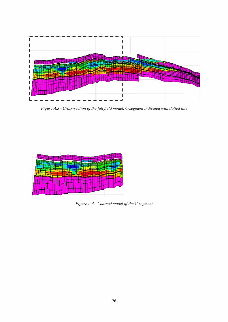
76
Figure A.3 - Cross-section of the full field model, C-segment indicated with dotted line
Figure A.4 - Coarsed model of the C-segment

77
Figure A.5 - Hydrocarbon composition at the Norne Field (Kalsnæs, 2010).

78

79
B. Screening table
Figure B.1 - Depicts the screening table (Taber, et al., 1997).

80

81
C. ECLIPSE 100
The datafile to be simulated by ECLIPSE is constructed in a special way. It is divided into
eight sections. These are RUNSPEC, GRID, EDIT, PROPS, REGIONS, SOLUTIONS,
SUMMARY and SCHEDULE and they need to be defined in that order (NTNU, 2011).
- RUNSPEC is a required section. This section states the title, problem dimensions, the
phases and components present in the model defined.
- GRID is the second section and is also required to be included in the datafile. The
geometry of the grid, used to model the reservoir, is defined at this stage. The various
rock properties, e.g. porosity and permeabilities, are specified for each grid block.
From this information ECLIPSE calculates the pore volumes, the mid-point depths of
all the grid blocks and the inter-block transmissibilities.
- EDIT is an optional section. Modifications to the calculated values in the grid section
can be modified in this segment.
- PROPS is a required section. This section includes tables of reservoir rock and fluids
as functions of fluid pressures, saturations and compositions i.e. density, viscosity,
relative permeability and capillary pressure.
- To include REGIONS in the datafile is optional. This is done if it is desirable for the
grid blocks to have different PVT properties, saturation properties, initial conditions
and amount of fluids in place.
- SOLUTION is a required section. It should contain specification of the initial
conditions in the reservoir model. The data includes pressure, saturations and
compositions of all the defined grid blocks.
- SUMMARY is optional to include. All of the data that is desirable to have written to
the output summary file should be defined in this section.
- SCHEDULE is the last section and needs to be defined. It specifies the operations to
be simulated and the times at which output reports are required.

82

83
D. Surfactant model
The next chapters contain information about these important features included by the
surfactant model.
The Capillary Number
The capillary number is previously defined in this project as the ratio of viscous to capillary
forces. It has also been discussed that it is desirable to have a high capillary number. ELIPSE
100 calculates the capillary number in the following way:
= | ∙ | (D.1)
Where K is the permeability, P is the potential, ST denotes the interfacial tension and Cunit is a
conversion factor depending on which units that are used. |K·gradP| is calculated in the
following way:
| ∙ | = ( ∙ ) + ∙ + ( ∙ ) (D.2)
∙ = 0.5 , ∙ ( − ) + , ∙ ( − ) (D.3)
The similar approach as for the x-direction is applied for the y- and z- direction
(Schlumberger, 2011).
Relative Permeability Model
The relative permeability data is given as input data for immiscible (no mixing) interaction
between oil and water. When surfactants are added to the system mixing will occur between
the water and the chemicals. Relative permeability data for this miscible phase will be
calculated from the given immiscible relative permeability data. These calculated data will
only be applied and used by the grid blocks that contain surfactants and thus miscibility will
be an option (Schlumberger, 2011).
Capillary Pressure
As mentioned previously the aim of a surfactant flooding is to lower the capillary pressure in
order to reduce the amount of trapped oil. The capillary pressure will decrease as the
concentration of surfactants increase during flooding. ECLIPSE calculates the pressure in the
following way (Schlumberger, 2011):

84
= ( ) (D.4)
Where Csurf is the concentration of surfactant, ST(Csurf) is the surface tension at the present
surfactant concentration and ST(Csurf = 0) is the surface tension when the concentration is
zero. Pc(Sw) is the capillary pressure from the immiscible curves scaled and calculated from
the miscible relative permeability model.
Water PVT Properties
When the surfactants mix with the water the viscosity of the water (pure or salted, depending
on the conditions in the reservoir) will be modified. To calculate the viscosity of the water-
surfactant phase ECLIPSE uses the following formula:
, = ( ) ( ) (D.5)
Where μ denotes viscosity and the subscript ws indicate water-surfactant solution, s indicate
surfactant and w indicate water. Pref is the reference pressure in the water. Csurf is the reference
salt concentration in the water if this is saline (Schlumberger, 2011).
Adsorption
Adsorption was in chapter 4.5.2 defined as one of the major factors contributing to surfactant
loss in a reservoir. ECLIPSE defines the quantity of absorbed surfactant as a function of
surrounding surfactant concentration. The absorbed mass is defined as follows:
= ∙ ∙ ∙ (D.6)
Where PVcell is the pore volume of the cell, ϕ is the porosity, MD is the mass density of the
rock and CA(Csurf) is the adsorption isotherm as a function of local surfactant concentration
solution (Schlumberger, 2011).

85
E. Keywords in the Surfactant Model
Within the eight sections explained in Appendix C there are some keywords that need to be
included in order to implement a surfactant flooding project in Eclipse.
SURFACT
This keyword is mentioned earlier as the word that activates the surfactant model. It should be
included in the RUNSPEC section (Schlumberger, 2011).
SURFST
This keyword must be included in order to successfully implement surfactant flooding. It
should be in the PROPS section. SURFST defines the interfacial tension between oil and
water as a function of the surfactant concentration (Schlumberger, 2011).
SURFVISC
This keyword is also required to be included in the model and should be defined in the
PROPS section. It is an abbreviation for surfactant solution viscosity function and is declared
by a table where values for the surfactant concentration are in the first column and the
associated water viscosities are defined in the second column (Schlumberger, 2011).
SURFCAPD
SURFCAPD defines the capillary desaturation function. It describes the transition between
immiscibility, which indicates low surfactant concentration, and miscibility, which indicate
high surfactant concentration, as a function of the capillary number. It is required to include
this in the PROPS section in a successful implementation of the surfactant model
(Schlumberger, 2011).
SURFADS
It is optional to include SURFADS in the PROPS section. This keyword defines the
adsorption and is highly recommended to include in the model to make it realistic. The
function is defined by a table where the first column states the concentration of surfactants in
solution and the second column states the concentration of surfactants absorbed by the rock
(Schlumberger, 2011).
SURFROCK
When the adsorption is included in the model it is required to include this keyword. It defines
the rock properties used by the surfactant model. The first column contains the so called

86
adsorption index. This is given the value 1 or 2 depending on whether desorbtion is allowed.
Desorption is the opposite of adsorption and indicated by defining 1 to be the index. The
second column contains the rock density at reservoir condition (Schlumberger, 2011). The
keyword should be included in the PROPS section.
WSURFACT
This keyword defines the concentration of surfactant to be injected into the reservoir. It is
included in the SCHEDULE section and only applies for the wells declared as water injectors.
The first column depicts the name of the water injector whilst the second column defines the
concentration as mass of surfactant per mass of water.

87
F. Surfactant input file SURFST -- Need as many tables as PVT tables, defined in the second keyword in TABDIMS = 2 -- Surfactant Water/oil Surface --conc., kg/m3 Tension, N/m 0 30.0E-03 0.1 10.0E-03 0.25 1.60E-03 0.5 0.40E-03 1.0 0.07E-03 3.0 0.006E-03 5.0 0.004E-03 10.0 0.003E-03 20.0 0.001E-03 / SURFVISC -- Need as many tables as PVT tables, defined in the second keyword in TABDIMS = 2 --Surf conc Water Viscosity --Kg/m3 Centipoise 0.0 0.318 5.0 0.449 10.0 0.503 15.0 0.540 20.0 0.630 / SURFADS -- Need as many tables as saturation tables, defined in the first keyword in TABDIMS = 107 --Surfactant Adsorption by rock --Surf conc Adsorbed mass --Kg/m3 (kg/kg) = kg surf /kg rock 0.0 0.00000 1.0 0.00017 5.0 0.00017 10.0 0.00017 / SURFCAPD -- Need as many tables as saturation tables, defined in the first keyword in TABDIMS = 107 --Capillary De-saturation curve --Log10 (capillary Miscibility --number) function 0 = immiscible, 1= miscible -8 0.0 -7 0.0 -6 0.0 -5.0 0.0 -2.5 1.0 0 1.0 5 1.0 10 1.0/ SURFROCK -- Need as many tables as saturation tables, defined in the first keyword in TABDIMS = 107 -- No desorption 1 2650/

88

89
G. Prediction input file --USER EVENT ZIPP2OFF GCONINJE 'FIELD' 'WATER' 'RATE' 47000.000 9* / / GCONPROD 'FIELD' 'ORAT' 36100.000 28500.000 7030000.000 36100.00 'RATE' 'NO' 8* / 'MANI-B2''LRAT' 9000.000 9000.000 3000000.000 9000.00 'RATE' 'YES' 8* / 'MANI-B1''LRAT' 9000.000 9000.000 2000000.000 9000.00 'RATE' 'YES' 8* / 'MANI-D1''LRAT' 9000.000 9000.000 2000000.000 9000.00 'RATE' 'YES' 8* / 'MANI-D2''LRAT' 9000.000 9000.000 2000000.000 9000.00 'RATE' 'YES' 8* / 'MANI-E1''LRAT' 9000.000 9000.000 2000000.000 9000.00 'RATE' 'YES' 8* / 'MANI-E2''LRAT' 9000.000 9000.000 2000000.000 9000.00 'RATE' 'YES' 8* / / GCONSALE 'FIELD' 2949000.000 2950000.000 2948000.000 'NONE' / / GUIDERAT 30.000 'OIL' 1.000 10.000 15.000 2.000 0.002 1.500 'YES' 1* / GCONSUMP 'FIELD' 441800.000 2* / / -- 3343.000000 days from start of simulation ( 6 'NOV' 1997 ) DATES 1 'JAN' 2007 / / WCONINJE 'C-1H' 'WATER' 'OPEN' 'RATE' 12000.000 3* 12 1* / 'C-2H' 'WATER' 'OPEN' 'RATE' 12000.000 3* 13 1* / 'C-3H' 'WATER' 'OPEN' 'RATE' 8000.000 3* 14 1* / / COMPDAT -- WELL I J K1 K2 Sat. CF DIAM KH SKIN ND DIR Ro 'C-1H' 26 44 5 5 'OPEN' 1* 4.787 0.216 446.775 2* 'Z' 16.040/ 'C-1H' 26 44 6 6 'OPEN' 1* 4.77 0.21 445.25 2* 'Z' 15.954/ 'C-1H' 26 44 7 7 'OPEN' 1* 6.53 0.21 609.083 2* 'Z' 15.888/ 'C-1H' 26 44 8 8 'OPEN' 1* 6.508 0.216 604.654 2* 'Z' 15.677/ 'C-1H' 26 44 9 9 'OPEN' 1* 52.636 0.216 4889.728 2* 'Z' 15.666/ 'C-1H' 26 44 10 10 'OPEN' 1*172.673 0.216 16014.438 2*'Z' 15.538/ 'C-1H' 26 44 11 11 'OPEN' 1* 13.370 0.216 1235.506 2*'Z' 15.263/ / COMPDAT -- WELL I J K1 K2 Sat. CF DIAM KH SKIN ND DIR Ro 'C-2H' 24 14 5 5 ‘OPEN' 1* 22.116 0.216 1988.961 2* 'Y’ 13.365/ 'C-2H' 24 14 6 6 'OPEN' 1* 25.523 0.216 2296.808 2* 'Y' 13.419/

90
'C-2H' 24 14 7 7 'OPEN' 1* 91.014 0.216 8165.169 2* 'Y' 13.209/ 'C-2H' 24 14 8 8 'OPEN 1* 0.357 0.216 31.636 2* ‘Y' 12.402/ ‘C-2H' 24 14 9 9 'OPEN' 1* 76.827 0.216 7207.936 2* 'Y’ 16.461/ 'C-2H' 24 14 10 10 'OPEN' 1* 76.827 0.216 7207.936 2* 'Y' 16.461/ 'C-2H' 24 14 11 11 'OPEN' 1* 76.827 0.216 7207.936 2* 'Y' 16.461/ 'C-2H' 24 14 12 12 'OPEN' 1* 22.116 0.216 1988.961 2* 'Y' 13.365/ / COMPDAT -- WELL I J K1 K2 Sat. CF DIAM KH SKIN ND DIR Ro 'C-3H' 9 13 5 5 'OPEN' 1* 15.871 0.216 1474.759 2* 'Z' 15.685/ ‘C-3H' 9 13 6 6 'OPEN' 1* 15.768 0.216 1467.264 2* 'Z' 15.796/ 'C-3H' 9 13 7 7 'OPEN' 1* 7.937 0.216 736.293 2* 'Z’ 15.554/ 'C-3H' 9 13 8 8 'OPEN' 1* 7.861 0.216 731.239 2* 'Z' 15.769/ 'C-3H' 9 13 9 9 'OPEN' 1* 21.934 0.216 2045.254 2* 'Z' 15.963/ 'C-3H' 9 13 10 10 'OPEN' 1* 115.228 0.216 10771.005 2* 'Z' 16.159/ 'C-3H' 9 13 11 11 'OPEN' 1* 32.211 0.216 3007.082 2* 'Z' 16.056/ / WSURFACT 'C-1H' 0 / 'C-2H' 10.0 / 'C-3H' 0 / / WCONINJE 'C-2H' 'WATER' 'OPEN' 'RATE' 10000.000 1* 1* 3* / / RPTSCHED 0 0 0 0 0 0 2 2 2 0 1 1 0 1 1 0 0 0 0 0 1 0 0 0 0 0 0 0 0 0 0 0 0 0 0 0 0 0 0 0 0 0 0 0 0 0 0 0 0 0 0 0 0 0 0 0 0 0 0 0 0 0 0 0 0 0 0 0 0 0 0 0 0 0 0 0 0 0 0 / -------------------------------------------------------------------- -- 3524.000000 days from start of simulation ( 6 'NOV' 1997 ) DATES 1 'JUL' 2007 / / RPTSCHED 0 0 0 0 0 0 2 2 2 0 1 1 0 1 1 0 0 0 0 0 1 0 0 0 0 0 0 0 0 0 0 0 0 0 0 0 0 0 0 0 0 0 0 0 0 0 0 0 0 0 0 0 0 0 0 0 0 0 0 0 0 0 0 0 0 0 0 0 0 0 0 0 0 0 0 0 0 0 0 / -------------------------------------------------------------------- -- 3708.000000 days from start of simulation ( 6 'NOV' 1997 ) DATES 1 'JAN' 2008 / / RPTSCHED 0 0 0 0 0 0 2 2 2 0 1 1 0 1 1 0 0 0 0 0 1 0 0 0 0 0 0 0 0 0 0 0 0 0 0 0 0 0 0 0 0 0 0 0 0 0 0 0 0 0 0 0 0 0 0 0 0 0 0 0 0 0

91
0 0 0 0 0 0 0 0 0 0 0 0 0 0 0 0 0 / -------------------------------------------------------------------- -- 3890.000000 days from start of simulation ( 6 'NOV' 1997 ) DATES 1 'JUL' 2008 / / RPTSCHED 0 0 0 0 0 0 2 2 2 0 1 1 0 1 1 0 0 0 0 0 1 0 0 0 0 0 0 0 0 0 0 0 0 0 0 0 0 0 0 0 0 0 0 0 0 0 0 0 0 0 0 0 0 0 0 0 0 0 0 0 0 0 0 0 0 0 0 0 0 0 0 0 0 0 0 0 0 0 0 / -------------------------------------------------------------------- -- 4074.000000 days from start of simulation ( 6 'NOV' 1997 ) DATES 1 'JAN' 2009 / / WSURFACT 'C-1H' 0.0 / 'C-2H' 0.0 / 'C-3H' 0.0 / / RPTSCHED 0 0 0 0 0 0 2 2 2 0 1 1 0 1 1 0 0 0 0 0 1 0 0 0 0 0 0 0 0 0 0 0 0 0 0 0 0 0 0 0 0 0 0 0 0 0 0 0 0 0 0 0 0 0 0 0 0 0 0 0 0 0 0 0 0 0 0 0 0 0 0 0 0 0 0 0 0 0 0 / -------------------------------------------------------------------- -- 4255.000000 days from start of simulation ( 6 'NOV' 1997 ) DATES 1 'JUL' 2009 / / RPTSCHED 0 0 0 0 0 0 2 2 2 0 1 1 0 1 1 0 0 / -------------------------------------------------------------------- -- 4439.000000 days from start of simulation ( 6 'NOV' 1997 ) DATES 1 'JAN' 2010 / / RPTSCHED 0 0 0 0 0 0 2 2 2 0 1 1 0 1 1 0 0 / -------------------------------------------------------------------- -- 4620.000000 days from start of simulation ( 6 'NOV' 1997 ) DATES 1 'JUL' 2010 / / RPTSCHED 0 0 0 0 0 0 2 2 2 0 1 1 0 1 1 0 0 / -------------------------------------------------------------------- -- 4804.000000 days from start of simulation ( 6 'NOV' 1997 )

92
DATES 1 'JAN' 2011 / / RPTSCHED 0 0 0 0 0 0 2 2 2 0 1 1 0 1 1 0 0 / -------------------------------------------------------------------- -- 4985.000000 days from start of simulation ( 6 'NOV' 1997 ) DATES 1 'JUL' 2011 / / RPTSCHED 0 0 0 0 0 0 2 2 2 0 1 1 0 1 1 0 0 / -------------------------------------------------------------------- -- 5169.000000 days from start of simulation ( 6 'NOV' 1997 ) DATES 1 'JAN' 2012 / / RPTSCHED 0 0 0 0 0 0 2 2 2 0 1 1 0 1 1 0 0 / -------------------------------------------------------------------- -- 5351.000000 days from start of simulation ( 6 'NOV' 1997 ) DATES 1 'JUL' 2012 / / RPTSCHED 0 0 0 0 0 0 2 2 2 0 1 1 0 1 1 0 0 / -------------------------------------------------------------------- -- 5535.000000 days from start of simulation ( 6 'NOV' 1997 ) DATES 1 'JAN' 2013 / / RPTSCHED 0 0 0 0 0 0 2 2 2 0 1 1 0 1 1 0 0 / -------------------------------------------------------------------- -- 5716.000000 days from start of simulation ( 6 'NOV' 1997 ) DATES 1 'JUL' 2013 / / RPTSCHED 0 0 0 0 0 0 2 2 2 0 1 1 0 1 1 0 0 / -------------------------------------------------------------------- -- 5900.000000 days from start of simulation ( 6 'NOV' 1997 ) DATES 1 'JAN' 2014 / / RPTSCHED 0 0 0 0 0 0 2 2 2 0 1 1 0 1 1 0 0 / -------------------------------------------------------------------- -- 6081.000000 days from start of simulation ( 6 'NOV' 1997 )

93
DATES 1 'JUL' 2014 / / RPTSCHED 0 0 0 0 0 0 2 2 2 0 1 1 0 1 1 0 0 / -------------------------------------------------------------------- -- 6265.000000 days from start of simulation ( 6 'NOV' 1997 ) DATES 1 'JAN' 2015 / / RPTSCHED 0 0 0 0 0 0 2 2 2 0 1 1 0 1 1 0 0 / -------------------------------------------------------------------- -- 6446.000000 days from start of simulation ( 6 'NOV' 1997 ) DATES 1 'JUL' 2015 / / RPTSCHED 0 0 0 0 0 0 2 2 2 0 1 1 0 1 1 0 0 / -------------------------------------------------------------------- -- 6630.000000 days from start of simulation ( 6 'NOV' 1997 ) DATES 1 'JAN' 2016 / / RPTSCHED 0 0 0 0 0 0 2 2 2 0 1 1 0 1 1 0 0 / -------------------------------------------------------------------- -- 6812.000000 days from start of simulation ( 6 'NOV' 1997 ) DATES 1 'JUL' 2016 / / RPTSCHED 0 0 0 0 0 0 2 2 2 0 1 1 0 1 1 0 0 / -------------------------------------------------------------------- -- 6996.000000 days from start of simulation ( 6 'NOV' 1997 ) DATES 1 'JAN' 2017 / / RPTSCHED 0 0 0 0 0 0 2 2 2 0 1 1 0 1 1 0 0 / -------------------------------------------------------------------- -- 7177.000000 days from start of simulation ( 6 'NOV' 1997 ) DATES 1 'JUL' 2017 / / RPTSCHED 0 0 0 0 0 0 2 2 2 0 1 1 0 1 1 0 0 /
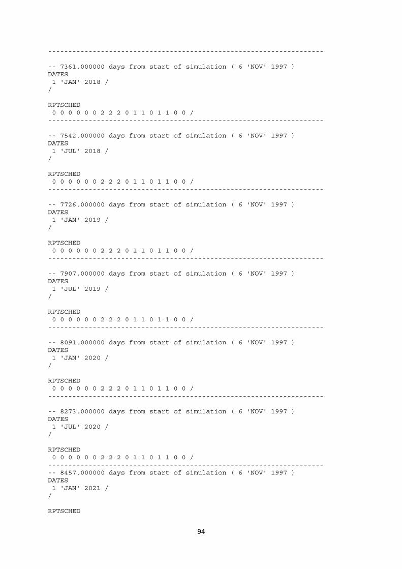
94
-------------------------------------------------------------------- -- 7361.000000 days from start of simulation ( 6 'NOV' 1997 ) DATES 1 'JAN' 2018 / / RPTSCHED 0 0 0 0 0 0 2 2 2 0 1 1 0 1 1 0 0 / -------------------------------------------------------------------- -- 7542.000000 days from start of simulation ( 6 'NOV' 1997 ) DATES 1 'JUL' 2018 / / RPTSCHED 0 0 0 0 0 0 2 2 2 0 1 1 0 1 1 0 0 / -------------------------------------------------------------------- -- 7726.000000 days from start of simulation ( 6 'NOV' 1997 ) DATES 1 'JAN' 2019 / / RPTSCHED 0 0 0 0 0 0 2 2 2 0 1 1 0 1 1 0 0 / -------------------------------------------------------------------- -- 7907.000000 days from start of simulation ( 6 'NOV' 1997 ) DATES 1 'JUL' 2019 / / RPTSCHED 0 0 0 0 0 0 2 2 2 0 1 1 0 1 1 0 0 / -------------------------------------------------------------------- -- 8091.000000 days from start of simulation ( 6 'NOV' 1997 ) DATES 1 'JAN' 2020 / / RPTSCHED 0 0 0 0 0 0 2 2 2 0 1 1 0 1 1 0 0 / -------------------------------------------------------------------- -- 8273.000000 days from start of simulation ( 6 'NOV' 1997 ) DATES 1 'JUL' 2020 / / RPTSCHED 0 0 0 0 0 0 2 2 2 0 1 1 0 1 1 0 0 / -------------------------------------------------------------------- -- 8457.000000 days from start of simulation ( 6 'NOV' 1997 ) DATES 1 'JAN' 2021 / / RPTSCHED

95
0 0 0 0 0 0 2 2 2 0 1 1 0 1 1 0 0 / -- 8638.000000 days from start of simulation ( 6 'NOV' 1997 ) DATES 1 'JUL' 2021 / / RPTSCHED 0 0 0 0 0 0 2 2 2 0 1 1 0 1 1 0 0 / -------------------------------------------------------------------- DATES 1 'JAN' 2022 / / -- END OF SIMULATION

96
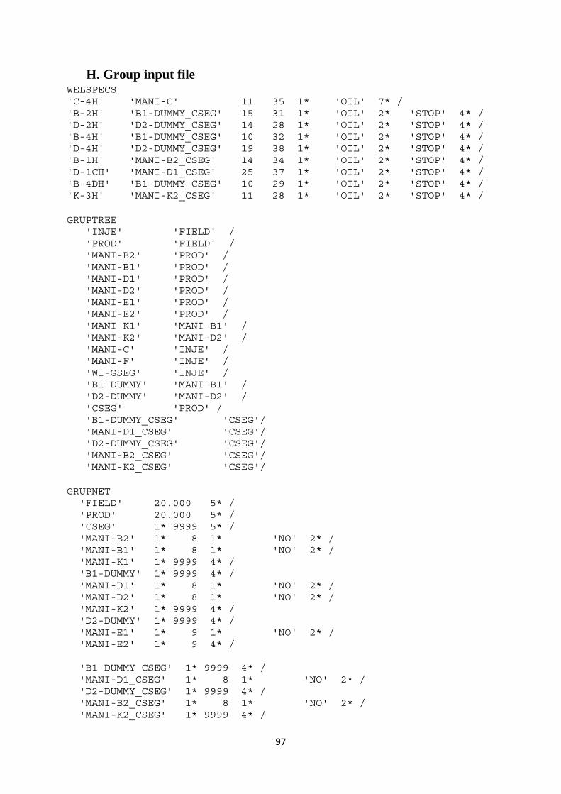
97
H. Group input file WELSPECS 'C-4H' 'MANI-C' 11 35 1* 'OIL' 7* / 'B-2H' 'B1-DUMMY_CSEG' 15 31 1* 'OIL' 2* 'STOP' 4* / 'D-2H' 'D2-DUMMY_CSEG' 14 28 1* 'OIL' 2* 'STOP' 4* / 'B-4H' 'B1-DUMMY_CSEG' 10 32 1* 'OIL' 2* 'STOP' 4* / 'D-4H' 'D2-DUMMY_CSEG' 19 38 1* 'OIL' 2* 'STOP' 4* / 'B-1H' 'MANI-B2_CSEG' 14 34 1* 'OIL' 2* 'STOP' 4* / 'D-1CH' 'MANI-D1_CSEG' 25 37 1* 'OIL' 2* 'STOP' 4* / 'B-4DH' 'B1-DUMMY_CSEG' 10 29 1* 'OIL' 2* 'STOP' 4* / 'K-3H' 'MANI-K2_CSEG' 11 28 1* 'OIL' 2* 'STOP' 4* / GRUPTREE 'INJE' 'FIELD' / 'PROD' 'FIELD' / 'MANI-B2' 'PROD' / 'MANI-B1' 'PROD' / 'MANI-D1' 'PROD' / 'MANI-D2' 'PROD' / 'MANI-E1' 'PROD' / 'MANI-E2' 'PROD' / 'MANI-K1' 'MANI-B1' / 'MANI-K2' 'MANI-D2' / 'MANI-C' 'INJE' / 'MANI-F' 'INJE' / 'WI-GSEG' 'INJE' / 'B1-DUMMY' 'MANI-B1' / 'D2-DUMMY' 'MANI-D2' / 'CSEG' 'PROD' / 'B1-DUMMY_CSEG' 'CSEG'/ 'MANI-D1_CSEG' 'CSEG'/ 'D2-DUMMY_CSEG' 'CSEG'/ 'MANI-B2_CSEG' 'CSEG'/ 'MANI-K2_CSEG' 'CSEG'/ GRUPNET 'FIELD' 20.000 5* / 'PROD' 20.000 5* / 'CSEG' 1* 9999 5* / 'MANI-B2' 1* 8 1* 'NO' 2* / 'MANI-B1' 1* 8 1* 'NO' 2* / 'MANI-K1' 1* 9999 4* / 'B1-DUMMY' 1* 9999 4* / 'MANI-D1' 1* 8 1* 'NO' 2* / 'MANI-D2' 1* 8 1* 'NO' 2* / 'MANI-K2' 1* 9999 4* / 'D2-DUMMY' 1* 9999 4* / 'MANI-E1' 1* 9 1* 'NO' 2* / 'MANI-E2' 1* 9 4* / 'B1-DUMMY_CSEG' 1* 9999 4* / 'MANI-D1_CSEG' 1* 8 1* 'NO' 2* / 'D2-DUMMY_CSEG' 1* 9999 4* / 'MANI-B2_CSEG' 1* 8 1* 'NO' 2* / 'MANI-K2_CSEG' 1* 9999 4* /

98

99
I. Region input file EQUALS
--Defined by Kristine Nielsen FIPILE 5 6 29 11 35 5 11 / FIPILE 5 7 29 36 37 5 11 / FIPILE 5 8 29 38 38 5 11 / FIPILE 5 9 29 39 41 5 11 / FIPILE 5 10 29 42 42 5 11 / FIPILE 5 11 29 43 44 5 11 / FIPILE 5 13 29 45 47 5 11 / FIPILE 5 20 29 48 48 5 11 / FIPILE 5 25 29 49 49 5 11 / FIPILE 6 6 6 36 42 5 11 / FIPILE 6 7 7 38 42 5 11 / FIPILE 6 8 8 39 42 5 11 / FIPILE 6 9 9 42 42 5 11 / FIPILE 6 10 10 43 44 5 11 / --Defined by Kristine Nielsen FIPTOFTE 9 6 29 11 35 12 18 / FIPTOFTE 9 7 29 36 37 12 18 / FIPTOFTE 9 8 29 38 38 12 18 / FIPTOFTE 9 9 29 39 41 12 18 / FIPTOFTE 9 10 29 42 42 12 18 / FIPTOFTE 9 11 29 43 44 12 18 / FIPTOFTE 9 13 29 45 47 12 18 / FIPTOFTE 9 20 29 48 48 12 18 / FIPTOFTE 9 25 29 49 49 12 18 / FIPTOFTE 10 6 6 36 42 12 18 / FIPTOFTE 10 7 7 38 42 12 18 / FIPTOFTE 10 8 8 39 42 12 18 / FIPTOFTE 10 9 9 42 42 12 18 / FIPTOFTE 10 10 10 43 44 12 18 /

100
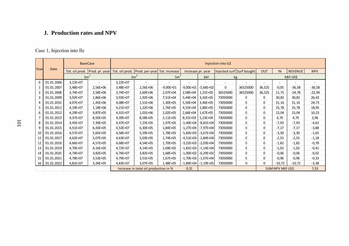
101
J. Production rates and NPV
Case 1, Injection into Ile
Tot. oil prod. Prod. pr. year Tot. oil prod. Prod. per year Tot. increase Injected surf Surf bought OUT IN REVENUE NPVbbl
0 01.01.2006 3,22E+07 - 3,22E+07 - - - - - - - - - -1 01.01.2007 3,48E+07 2,56E+06 3,48E+07 2,56E+06 -9,00E+01 -9,00E+01 -5,66E+02 0 36525000 36,525 -0,05 -36,58 -36,582 01.01.2008 3,74E+07 2,58E+06 3,74E+07 2,60E+06 2,07E+04 2,08E+04 1,31E+05 36525000 36525000 36,525 11,75 -24,78 -22,943 01.01.2009 3,92E+07 1,86E+06 3,93E+07 1,92E+06 7,51E+04 5,44E+04 3,42E+05 73050000 0 0 30,82 30,82 26,424 01.01.2010 4,07E+07 1,45E+06 4,08E+07 1,51E+06 1,30E+05 5,50E+04 3,46E+05 73050000 0 0 31,16 31,16 24,735 01.01.2011 4,19E+07 1,18E+06 4,21E+07 1,22E+06 1,76E+05 4,55E+04 2,86E+05 73050000 0 0 25,78 25,78 18,956 01.01.2012 4,29E+07 9,87E+05 4,31E+07 1,01E+06 2,02E+05 2,66E+04 1,67E+05 73050000 0 0 15,04 15,04 10,237 01.01.2013 4,37E+07 8,50E+05 4,39E+07 8,58E+05 2,11E+05 8,31E+03 5,23E+04 73050000 0 0 4,70 4,70 2,968 01.01.2014 4,45E+07 7,39E+05 4,47E+07 7,25E+05 1,97E+05 -1,40E+04 -8,81E+04 73050000 0 0 -7,93 -7,93 -4,639 01.01.2015 4,51E+07 6,43E+05 4,53E+07 6,30E+05 1,84E+05 -1,27E+04 -7,97E+04 73050000 0 0 -7,17 -7,17 -3,88
10 01.01.2016 4,57E+07 5,65E+05 4,58E+07 5,59E+05 1,78E+05 -5,83E+03 -3,67E+04 73050000 0 0 -3,30 -3,30 -1,6511 01.01.2017 4,62E+07 5,07E+05 4,63E+07 5,03E+05 1,74E+05 -4,51E+03 -2,84E+04 73050000 0 0 -2,55 -2,55 -1,1812 01.01.2018 4,66E+07 4,57E+05 4,68E+07 4,54E+05 1,70E+05 -3,22E+03 -2,03E+04 73050000 0 0 -1,82 -1,82 -0,7813 01.01.2019 4,70E+07 4,16E+05 4,72E+07 4,14E+05 1,69E+05 -1,81E+03 -1,14E+04 73050000 0 0 -1,02 -1,02 -0,4114 01.01.2020 4,74E+07 3,82E+05 4,76E+07 3,82E+05 1,68E+05 -1,00E+02 -6,29E+02 73050000 0 0 -0,06 -0,06 -0,0215 01.01.2021 4,78E+07 3,53E+05 4,79E+07 3,51E+05 1,67E+05 -1,70E+03 -1,07E+04 73050000 0 0 -0,96 -0,96 -0,3316 01.01.2022 4,81E+07 3,26E+05 4,83E+07 3,07E+05 1,48E+05 -1,89E+04 -1,19E+05 73050000 0 0 -10,72 -10,72 -3,38
0,31 SUM NPV Mill US$ 7,53Increase in total oil production in %
Year DateBaseCase Injection into ILE
Increase pr. yearSm3 Sm3 Sm3 kg Mill US$

102
Case 1, Injection into Tofte
Tot. oil prod. Prod. pr. year Tot. oil prod. Prod. per year Tot. increase Injected surf Surf bought OUT IN REVENUE NPVbbl
0 01.01.2006 3,22E+07 - 3,22E+07 - - - - - - - - - -1 01.01.2007 3,48E+07 2,56E+06 3,48E+07 2,56E+06 -9,00E+01 -9,00E+01 -5,66E+02 0 36525000 36,525 -0,05 -36,58 -36,582 01.01.2008 3,74E+07 2,55E+06 3,74E+07 2,55E+06 1,07E+03 1,16E+03 7,30E+03 36525000 36525000 36,525 0,66 -35,87 -33,213 01.01.2009 3,92E+07 1,81E+06 3,92E+07 1,81E+06 -2,98E+03 -4,05E+03 -2,55E+04 73050000 0 0 -2,29 -2,29 -1,974 01.01.2010 4,06E+07 1,40E+06 4,06E+07 1,39E+06 -6,69E+03 -3,71E+03 -2,33E+04 73050000 0 0 -2,10 -2,10 -1,675 01.01.2011 4,17E+07 1,12E+06 4,17E+07 1,13E+06 -1,67E+03 5,02E+03 3,16E+04 73050000 0 0 2,84 2,84 2,096 01.01.2012 4,26E+07 9,32E+05 4,26E+07 9,41E+05 7,33E+03 9,00E+03 5,66E+04 73050000 0 0 5,09 5,09 3,477 01.01.2013 4,34E+07 8,00E+05 4,34E+07 8,15E+05 2,18E+04 1,45E+04 9,09E+04 73050000 0 0 8,18 8,18 5,158 01.01.2014 4,41E+07 7,01E+05 4,42E+07 7,14E+05 3,43E+04 1,25E+04 7,86E+04 73050000 0 0 7,08 7,08 4,139 01.01.2015 4,47E+07 6,19E+05 4,48E+07 6,33E+05 4,90E+04 1,47E+04 9,25E+04 73050000 0 0 8,32 8,32 4,50
10 01.01.2016 4,53E+07 5,51E+05 4,54E+07 5,65E+05 6,30E+04 1,40E+04 8,81E+04 73050000 0 0 7,93 7,93 3,9711 01.01.2017 4,58E+07 4,93E+05 4,59E+07 5,11E+05 8,01E+04 1,71E+04 1,08E+05 73050000 0 0 9,69 9,69 4,4912 01.01.2018 4,62E+07 4,44E+05 4,63E+07 4,66E+05 1,02E+05 2,17E+04 1,36E+05 73050000 0 0 12,28 12,28 5,2713 01.01.2019 4,66E+07 4,07E+05 4,68E+07 4,27E+05 1,22E+05 2,03E+04 1,28E+05 73050000 0 0 11,51 11,51 4,5714 01.01.2020 4,70E+07 3,75E+05 4,72E+07 3,94E+05 1,41E+05 1,88E+04 1,18E+05 73050000 0 0 10,64 10,64 3,9115 01.01.2021 4,74E+07 3,48E+05 4,75E+07 3,64E+05 1,57E+05 1,61E+04 1,01E+05 73050000 0 0 9,12 9,12 3,1016 01.01.2022 4,77E+07 3,24E+05 4,79E+07 3,36E+05 1,69E+05 1,24E+04 7,82E+04 73050000 0 0 7,04 7,04 2,22
0,36 SUM NPV Mill US$ -26,55
Mill US$
Increase in total oil production in %
Year DateBaseCase Injection into TOFTE
Increase pr. yearSm3 Sm3 Sm3 kg

103
Case 2, Injecting through C-1H
Tot. oil prod. Prod. pr. year Tot. oil prod. Prod. per year Tot. increase Injected surf Surf bought OUT IN REVENUE NPVbbl
0 01.01.2006 3,22E+07 - 3,22E+07 - - - - - - - - - -
1 01.01.2007 3,48E+07 2,56E+06 3,48E+07 2,56E+06 -9,00E+01 -9,00E+01 -5,66E+02 0 36525000 36,525 -0,06 -36,58 -36,582 01.01.2008 3,74E+07 2,58E+06 3,74E+07 2,58E+06 -1,17E+03 -1,08E+03 -6,79E+03 36525000 36525000 36,525 -0,68 -37,20 -34,453 01.01.2009 3,92E+07 1,86E+06 3,93E+07 1,87E+06 5,14E+03 6,31E+03 3,97E+04 73050000 36525000 36,525 3,97 -32,56 -27,914 01.01.2010 4,07E+07 1,45E+06 4,07E+07 1,45E+06 8,36E+03 3,22E+03 2,03E+04 109575000 36525000 36,525 2,03 -34,50 -27,395 01.01.2011 4,19E+07 1,18E+06 4,19E+07 1,19E+06 1,70E+04 8,66E+03 5,45E+04 146100000 36525000 36,525 5,45 -31,08 -22,846 01.01.2012 4,29E+07 9,87E+05 4,29E+07 1,00E+06 3,49E+04 1,79E+04 1,13E+05 182625000 36525000 36,525 11,25 -25,27 -17,207 01.01.2013 4,37E+07 8,50E+05 4,38E+07 8,78E+05 6,27E+04 2,78E+04 1,75E+05 219150000 36525000 36,525 17,45 -19,07 -12,028 01.01.2014 4,45E+07 7,39E+05 4,45E+07 7,69E+05 9,28E+04 3,01E+04 1,89E+05 255675000 36525000 36,525 18,95 -17,58 -10,269 01.01.2015 4,51E+07 6,43E+05 4,52E+07 6,77E+05 1,27E+05 3,46E+04 2,18E+05 292200000 36525000 36,525 21,78 -14,74 -7,97
10 01.01.2016 4,57E+07 5,65E+05 4,58E+07 6,03E+05 1,66E+05 3,84E+04 2,41E+05 328725000 36525000 36,525 24,12 -12,40 -6,2011 01.01.2017 4,62E+07 5,07E+05 4,64E+07 5,49E+05 2,08E+05 4,19E+04 2,64E+05 365250000 36525000 36,525 26,37 -10,15 -4,7012 01.01.2018 4,66E+07 4,57E+05 4,69E+07 5,01E+05 2,51E+05 4,33E+04 2,73E+05 401775000 36525000 36,525 27,26 -9,26 -3,9713 01.01.2019 4,70E+07 4,16E+05 4,73E+07 4,60E+05 2,95E+05 4,38E+04 2,75E+05 438300000 36525000 36,525 27,54 -8,99 -3,5714 01.01.2020 4,74E+07 3,82E+05 4,78E+07 4,20E+05 3,33E+05 3,83E+04 2,41E+05 474825000 36525000 36,525 24,06 -12,47 -4,5815 01.01.2021 4,78E+07 3,53E+05 4,81E+07 3,85E+05 3,65E+05 3,17E+04 1,99E+05 511350000 36525000 36,525 19,94 -16,59 -5,6516 01.01.2022 4,81E+07 3,26E+05 4,85E+07 3,54E+05 3,92E+05 2,76E+04 1,74E+05 547875000 0 0 17,38 17,38 5,48
0,82 SUM NPV Mill US$ -219,81Increase in total oil production in %
DateYearBaseCase C-1H
Sm3 Sm3 Sm3 kgIncrease pr. year
Mill US$
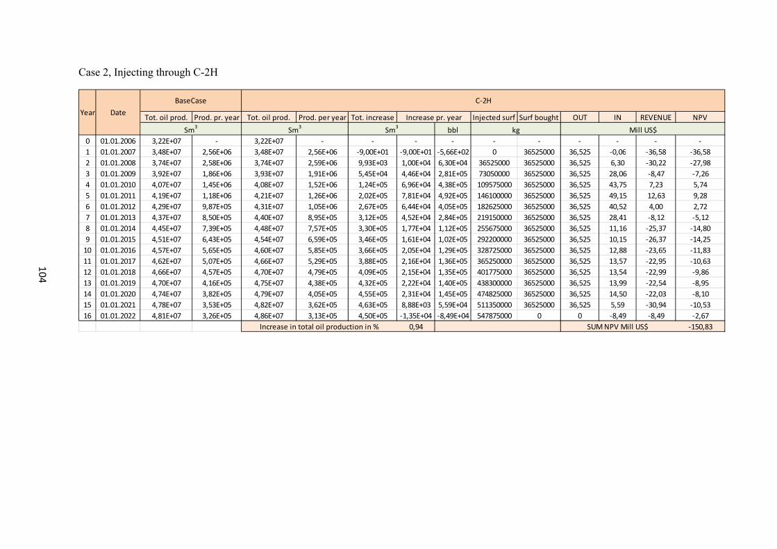
104
Case 2, Injecting through C-2H
Tot. oil prod. Prod. pr. year Tot. oil prod. Prod. per year Tot. increase Injected surf Surf bought OUT IN REVENUE NPVbbl
0 01.01.2006 3,22E+07 - 3,22E+07 - - - - - - - - - -1 01.01.2007 3,48E+07 2,56E+06 3,48E+07 2,56E+06 -9,00E+01 -9,00E+01 -5,66E+02 0 36525000 36,525 -0,06 -36,58 -36,582 01.01.2008 3,74E+07 2,58E+06 3,74E+07 2,59E+06 9,93E+03 1,00E+04 6,30E+04 36525000 36525000 36,525 6,30 -30,22 -27,983 01.01.2009 3,92E+07 1,86E+06 3,93E+07 1,91E+06 5,45E+04 4,46E+04 2,81E+05 73050000 36525000 36,525 28,06 -8,47 -7,264 01.01.2010 4,07E+07 1,45E+06 4,08E+07 1,52E+06 1,24E+05 6,96E+04 4,38E+05 109575000 36525000 36,525 43,75 7,23 5,745 01.01.2011 4,19E+07 1,18E+06 4,21E+07 1,26E+06 2,02E+05 7,81E+04 4,92E+05 146100000 36525000 36,525 49,15 12,63 9,286 01.01.2012 4,29E+07 9,87E+05 4,31E+07 1,05E+06 2,67E+05 6,44E+04 4,05E+05 182625000 36525000 36,525 40,52 4,00 2,727 01.01.2013 4,37E+07 8,50E+05 4,40E+07 8,95E+05 3,12E+05 4,52E+04 2,84E+05 219150000 36525000 36,525 28,41 -8,12 -5,128 01.01.2014 4,45E+07 7,39E+05 4,48E+07 7,57E+05 3,30E+05 1,77E+04 1,12E+05 255675000 36525000 36,525 11,16 -25,37 -14,809 01.01.2015 4,51E+07 6,43E+05 4,54E+07 6,59E+05 3,46E+05 1,61E+04 1,02E+05 292200000 36525000 36,525 10,15 -26,37 -14,25
10 01.01.2016 4,57E+07 5,65E+05 4,60E+07 5,85E+05 3,66E+05 2,05E+04 1,29E+05 328725000 36525000 36,525 12,88 -23,65 -11,8311 01.01.2017 4,62E+07 5,07E+05 4,66E+07 5,29E+05 3,88E+05 2,16E+04 1,36E+05 365250000 36525000 36,525 13,57 -22,95 -10,6312 01.01.2018 4,66E+07 4,57E+05 4,70E+07 4,79E+05 4,09E+05 2,15E+04 1,35E+05 401775000 36525000 36,525 13,54 -22,99 -9,8613 01.01.2019 4,70E+07 4,16E+05 4,75E+07 4,38E+05 4,32E+05 2,22E+04 1,40E+05 438300000 36525000 36,525 13,99 -22,54 -8,9514 01.01.2020 4,74E+07 3,82E+05 4,79E+07 4,05E+05 4,55E+05 2,31E+04 1,45E+05 474825000 36525000 36,525 14,50 -22,03 -8,1015 01.01.2021 4,78E+07 3,53E+05 4,82E+07 3,62E+05 4,63E+05 8,88E+03 5,59E+04 511350000 36525000 36,525 5,59 -30,94 -10,5316 01.01.2022 4,81E+07 3,26E+05 4,86E+07 3,13E+05 4,50E+05 -1,35E+04 -8,49E+04 547875000 0 0 -8,49 -8,49 -2,67
0,94 SUM NPV Mill US$ -150,83Increase in total oil production in %
Year DateBaseCase C-2H
Increase pr. yearSm3 Sm3 Sm3 kg Mill US$

105
Case 2, Injecting through C-3H
Total oil prod. Prod. pr. year Total oil prod. Prod. per year Total increase Injected surf Surf bought OUT IN REVENUE NPVbbl
0 01.01.2006 3,22E+07 3,22E+07 - - - - - - - - - -1 01.01.2007 3,48E+07 2,56E+06 3,48E+07 2,56E+06 -9,00E+01 -9,00E+01 -5,66E+02 0 36525000 36,525 -0,06 -36,58 -33,872 01.01.2008 3,74E+07 2,58E+06 3,74E+07 2,59E+06 1,12E+04 1,12E+04 7,07E+04 36525000 36525000 36,525 7,07 -29,46 -25,253 01.01.2009 3,92E+07 1,86E+06 3,92E+07 1,83E+06 -2,49E+04 -3,60E+04 -2,27E+05 73050000 36525000 36,525 -22,65 -59,18 -46,984 01.01.2010 4,07E+07 1,45E+06 4,07E+07 1,44E+06 -3,74E+04 -1,25E+04 -7,87E+04 109575000 36525000 36,525 -7,87 -44,39 -32,635 01.01.2011 4,19E+07 1,18E+06 4,18E+07 1,18E+06 -3,53E+04 2,11E+03 1,33E+04 146100000 36525000 36,525 1,33 -35,20 -23,966 01.01.2012 4,29E+07 9,87E+05 4,28E+07 9,95E+05 -2,77E+04 7,54E+03 4,74E+04 182625000 36525000 36,525 4,74 -31,78 -20,037 01.01.2013 4,37E+07 8,50E+05 4,37E+07 8,60E+05 -1,76E+04 1,02E+04 6,39E+04 219150000 36525000 36,525 6,39 -30,13 -17,588 01.01.2014 4,45E+07 7,39E+05 4,44E+07 7,42E+05 -1,45E+04 3,08E+03 1,94E+04 255675000 36525000 36,525 1,94 -34,59 -18,699 01.01.2015 4,51E+07 6,43E+05 4,51E+07 6,45E+05 -1,20E+04 2,53E+03 1,59E+04 292200000 36525000 36,525 1,59 -34,93 -17,48
10 01.01.2016 4,57E+07 5,65E+05 4,57E+07 5,72E+05 -4,51E+03 7,44E+03 4,68E+04 328725000 36525000 36,525 4,68 -31,85 -14,7511 01.01.2017 4,62E+07 5,07E+05 4,62E+07 5,14E+05 2,14E+03 6,65E+03 4,18E+04 365250000 36525000 36,525 4,18 -32,34 -13,8712 01.01.2018 4,66E+07 4,57E+05 4,66E+07 4,64E+05 8,53E+03 6,39E+03 4,02E+04 401775000 36525000 36,525 4,02 -32,51 -12,9113 01.01.2019 4,70E+07 4,16E+05 4,71E+07 4,23E+05 1,50E+04 6,51E+03 4,09E+04 438300000 36525000 36,525 4,09 -32,43 -11,9214 01.01.2020 4,74E+07 3,82E+05 4,74E+07 3,88E+05 2,11E+04 6,01E+03 3,78E+04 474825000 36525000 36,525 3,78 -32,74 -11,1515 01.01.2021 4,78E+07 3,53E+05 4,78E+07 3,60E+05 2,81E+04 7,08E+03 4,45E+04 511350000 36525000 36,525 4,45 -32,07 -10,1116 01.01.2022 4,81E+07 3,26E+05 4,81E+07 3,34E+05 3,66E+04 8,48E+03 5,33E+04 547875000 36525000 36,525 5,33 -31,19 -9,10
0,08 SUM NPV Mill US$ -320,28Increase in total oil production in %
Year DateBaseCase C-3H
Increase pr. yearSm3 Sm3 Sm3 kg Mill US$

106
Case 2, Injecting through all wells
Total oil prod. Prod. pr. year Total oil prod. Prod. per year Total increase Injected surf Surf bought OUT IN REVENUE NPVbbl
0 01.01.2006 3,22E+07 - 3,22E+07 - - - - - - - - - -1 01.01.2007 3,48E+07 2559390 3,48E+07 2559300 -9,00E+01 -90 29751,7 0 109575000 109,575 2,98 -106,60 -98,702 01.01.2008 3,74E+07 2583310 3,74E+07 2588040 4,64E+03 4730 -29122,7 109575000 109575000 109,575 -2,91 -112,49 -96,443 01.01.2009 3,92E+07 1861310 3,92E+07 1856680 1,00E+01 -4630 16228,2 219150000 109575000 109,575 1,62 -107,95 -85,704 01.01.2010 4,07E+07 1451320 4,07E+07 1453900 2,59E+03 2580 128756,3 328725000 109575000 109,575 12,88 -96,70 -71,085 01.01.2011 4,19E+07 1177820 4,19E+07 1198290 2,31E+04 20470 226691,6 438300000 109575000 109,575 22,67 -86,91 -59,156 01.01.2012 4,29E+07 986970 4,29E+07 1023010 5,91E+04 36040 283112,9 547875000 109575000 109,575 28,31 -81,26 -51,217 01.01.2013 4,37E+07 849830 4,38E+07 894840 1,04E+05 45010 327709 657450000 109575000 109,575 32,77 -76,80 -44,818 01.01.2014 4,45E+07 738910 4,46E+07 791010 1,56E+05 52100 336640,8 767025000 109575000 109,575 33,66 -75,91 -41,019 01.01.2015 4,51E+07 642800 4,53E+07 696320 2,10E+05 53520 353938,3 876600000 109575000 109,575 35,39 -74,18 -37,11
10 01.01.2016 4,57E+07 565010 4,59E+07 621280 2,66E+05 56270 365197,4 986175000 109575000 109,575 36,52 -73,06 -33,8411 01.01.2017 4,62E+07 507050 4,65E+07 565110 3,24E+05 58060 365700,6 1095750000 109575000 109,575 36,57 -73,00 -31,3112 01.01.2018 4,66E+07 457180 4,70E+07 515320 3,82E+05 58140 362115,3 1205325000 109575000 109,575 36,21 -73,36 -29,1313 01.01.2019 4,70E+07 416180 4,75E+07 473750 4,40E+05 57570 343245,3 1314900000 109575000 109,575 34,32 -75,25 -27,6714 01.01.2020 4,74E+07 381980 4,79E+07 436550 4,94E+05 54570 327080 1424475000 109575000 109,575 32,71 -76,87 -26,1715 01.01.2021 4,78E+07 353020 4,83E+07 405020 5,46E+05 52000 284874,1 1534050000 109575000 109,575 28,49 -81,09 -25,5616 01.01.2022 4,81E+07 326000 4,87E+07 371290 5,92E+05 45290 284874,1 1643625000 0 0 28,49 28,49 8,32
1,23 SUM NPV Mill US$ -750,58Increase in total oil production in %
Year DateBaseCase All Wells
Increase pr. yearSm3 Sm3 Sm3 kg Mill US$

107
Case 3, Using a surfactant concentration of 5 kg/Sm3
Tot. oil prod. Prod. pr. year Tot. oil prod. Prod. per year Tot. increase Injected surf Surf bought OUT IN REVENUE NPVbbl
0 01.01.2006 3,22E+07 - 3,22E+07 - - - - - - - - - -1 01.01.2007 3,48E+07 2,56E+06 3,48E+07 2,56E+06 -90 -90 -566,1 0 18262500 18,26 -0,06 -18,32 -18,322 01.01.2008 3,74E+07 2,58E+06 3,74E+07 2,60E+06 12240 12330 77555,7 18262500 18262500 18,26 7,76 -10,51 -9,733 01.01.2009 3,92E+07 1,86E+06 3,93E+07 1,91E+06 59310 47070 296070,3 36525000 18262500 18,26 29,61 11,34 9,734 01.01.2010 4,07E+07 1,45E+06 4,08E+07 1,52E+06 124300 64990 408787,1 54787500 18262500 18,26 40,88 22,62 17,955 01.01.2011 4,19E+07 1,18E+06 4,21E+07 1,24E+06 1,89E+05 65120 409604,8 73050000 18262500 18,26 40,96 22,70 16,686 01.01.2012 4,29E+07 9,87E+05 4,31E+07 1,04E+06 2,39E+05 49450 311040,5 91312500 18262500 18,26 31,10 12,84 8,747 01.01.2013 4,37E+07 8,50E+05 4,40E+07 8,79E+05 268200 29330 184485,7 109575000 18262500 18,26 18,45 0,19 0,128 01.01.2014 4,45E+07 7,39E+05 4,47E+07 7,43E+05 271910 3710 23335,9 127837500 18262500 18,26 2,33 -15,93 -9,299 01.01.2015 4,51E+07 6,43E+05 4,54E+07 6,44E+05 273590 1680 10567,2 146100000 18262500 18,26 1,06 -17,21 -9,3010 01.01.2016 4,57E+07 5,65E+05 4,59E+07 5,71E+05 279920 6330 39815,7 164362500 18262500 18,26 3,98 -14,28 -7,1411 01.01.2017 4,62E+07 5,07E+05 4,65E+07 5,14E+05 286440 6520 41010,8 182625000 18262500 18,26 4,10 -14,16 -6,5612 01.01.2018 4,66E+07 4,57E+05 4,69E+07 4,64E+05 293390 6950 43715,5 200887500 18262500 18,26 4,37 -13,89 -5,9613 01.01.2019 4,70E+07 4,16E+05 4,73E+07 4,24E+05 301640 8250 51892,5 219150000 18262500 18,26 5,19 -13,07 -5,1914 01.01.2020 4,74E+07 3,82E+05 4,77E+07 3,92E+05 311850 10210 64220,9 237412500 18262500 18,26 6,42 -11,84 -4,3515 01.01.2021 4,78E+07 3,53E+05 4,81E+07 3,52E+05 310890 -960 -6038,4 255675000 18262500 18,26 -0,60 -18,87 -6,4216 01.01.2022 4,81E+07 3,26E+05 4,84E+07 3,05E+05 290070 -20820 -130957,8 273937500 0 0,00 -13,10 -13,10 -4,13
0,60 SUM NPV Mill US$ -33,18
Increase pr. yearSm3
Increase in total oil production in %
Sm3 Sm3 kg Mill US$
Year DateBaseCase Surf. concentration = 5 kg/Sm3

108
Case 3, Using a surfactant concentration of 10 kg/Sm3
Tot. oil prod. Prod pr. year Tot. oil prod. Prod. per year Tot. increase Injected surf Surf bought OUT IN REVENUE NPV
bbl0 01.01.2006 3,22E+07 - 3,22E+07 - - - - - - - - - -1 01.01.2007 3,48E+07 2,56E+06 3,48E+07 2,56E+06 -90 -9,00E+01 -5,66E+02 0 36525000 36,53 -0,06 -36,58 -36,582 01.01.2008 3,74E+07 2,58E+06 3,74E+07 2,59E+06 9930 1,00E+04 6,30E+04 36525000 36525000 36,53 6,30 -30,22 -27,983 01.01.2009 3,92E+07 1,86E+06 3,93E+07 1,91E+06 54540 4,46E+04 2,81E+05 73050000 36525000 36,53 28,06 -8,47 -7,264 01.01.2010 4,07E+07 1,45E+06 4,08E+07 1,52E+06 124100 6,96E+04 4,38E+05 109575000 36525000 36,53 43,75 7,23 5,745 01.01.2011 4,19E+07 1,18E+06 4,21E+07 1,26E+06 202240 7,81E+04 4,92E+05 146100000 36525000 36,53 49,15 12,63 9,286 01.01.2012 4,29E+07 9,87E+05 4,31E+07 1,05E+06 266660 6,44E+04 4,05E+05 182625000 36525000 36,53 40,52 4,00 2,727 01.01.2013 4,37E+07 8,50E+05 4,40E+07 8,95E+05 311820 4,52E+04 2,84E+05 219150000 36525000 36,53 28,41 -8,12 -5,128 01.01.2014 4,45E+07 7,39E+05 4,48E+07 7,57E+05 329560 1,77E+04 1,12E+05 255675000 36525000 36,53 11,16 -25,37 -14,809 01.01.2015 4,51E+07 6,43E+05 4,54E+07 6,59E+05 345700 1,61E+04 1,02E+05 292200000 36525000 36,53 10,15 -26,37 -14,2510 01.01.2016 4,57E+07 5,65E+05 4,60E+07 5,85E+05 366170 2,05E+04 1,29E+05 328725000 36525000 36,53 12,88 -23,65 -11,8311 01.01.2017 4,62E+07 5,07E+05 4,66E+07 5,29E+05 387750 2,16E+04 1,36E+05 365250000 36525000 36,53 13,57 -22,95 -10,6312 01.01.2018 4,66E+07 4,57E+05 4,70E+07 4,79E+05 409270 2,15E+04 1,35E+05 401775000 36525000 36,53 13,54 -22,99 -9,8613 01.01.2019 4,70E+07 4,16E+05 4,75E+07 4,38E+05 431510 2,22E+04 1,40E+05 438300000 36525000 36,53 13,99 -22,54 -8,9514 01.01.2020 4,74E+07 3,82E+05 4,79E+07 4,05E+05 454560 2,31E+04 1,45E+05 474825000 36525000 36,53 14,50 -22,03 -8,1015 01.01.2021 4,78E+07 3,53E+05 4,82E+07 3,62E+05 463440 8,88E+03 5,59E+04 511350000 36525000 36,53 5,59 -30,94 -10,5316 01.01.2022 4,81E+07 3,26E+05 4,86E+07 3,13E+05 449950 -1,35E+04 -8,49E+04 547875000 0 0,00 -8,49 -8,49 -2,67
0,94 SUM NPV Mill US$ -150,83
kg Mill US$
Increase in total oil production in %
Year Date
BaseCase Surf. concentration = 10 kg/Sm3
Increase pr. year
Sm3 Sm3 Sm3

109
Case 3, Using a surfactant concentration of 30 kg/Sm3
Tot. oil prod. Prod pr. year Tot. oil prod. Prod. per year Tot. increase Injected surf Surf bought OUT IN REVENUE NPVbbl
0 01.01.2006 3,22E+07 - 3,22E+07 - - - - - - - - - -1 01.01.2007 3,48E+07 2,56E+06 3,48E+07 2,56E+06 -9,00E+01 -9,00E+01 -5,66E+02 0 109575000 109,58 -0,06 -109,63 -109,632 01.01.2008 3,74E+07 2,58E+06 3,74E+07 2,60E+06 14620 1,47E+04 9,25E+04 109575000 109575000 109,58 9,25 -100,32 -92,893 01.01.2009 3,92E+07 1,86E+06 3,93E+07 1,92E+06 73290 5,87E+04 3,69E+05 219150000 109575000 109,58 36,90 -72,67 -62,304 01.01.2010 4,07E+07 1,45E+06 4,09E+07 1,56E+06 177100 1,04E+05 6,53E+05 328725000 109575000 109,58 65,30 -44,28 -35,155 01.01.2011 4,19E+07 1,18E+06 4,22E+07 1,29E+06 292080 1,15E+05 7,23E+05 438300000 109575000 109,58 72,32 -37,25 -27,386 01.01.2012 4,29E+07 9,87E+05 4,33E+07 1,08E+06 386450 9,44E+04 5,94E+05 547875000 109575000 109,58 59,36 -50,22 -34,187 01.01.2013 4,37E+07 8,50E+05 4,42E+07 9,16E+05 452320 6,59E+04 4,14E+05 657450000 109575000 109,58 41,43 -68,14 -42,948 01.01.2014 4,45E+07 7,39E+05 4,49E+07 7,74E+05 487290 3,50E+04 2,20E+05 767025000 109575000 109,58 22,00 -87,58 -51,109 01.01.2015 4,51E+07 6,43E+05 4,56E+07 6,77E+05 521810 3,45E+04 2,17E+05 876600000 109575000 109,58 21,71 -87,86 -47,4710 01.01.2016 4,57E+07 5,65E+05 4,62E+07 6,03E+05 560270 3,85E+04 2,42E+05 986175000 109575000 109,58 24,19 -85,38 -42,7111 01.01.2017 4,62E+07 5,07E+05 4,68E+07 5,46E+05 599030 3,88E+04 2,44E+05 1095750000 109575000 109,58 24,38 -85,19 -39,4612 01.01.2018 4,66E+07 4,57E+05 4,73E+07 4,96E+05 637930 3,89E+04 2,45E+05 1205325000 109575000 109,58 24,47 -85,11 -36,5013 01.01.2019 4,70E+07 4,16E+05 4,77E+07 4,56E+05 678030 4,01E+04 2,52E+05 1314900000 109575000 109,58 25,22 -84,35 -33,5014 01.01.2020 4,74E+07 3,82E+05 4,81E+07 4,17E+05 712890 3,49E+04 2,19E+05 1424475000 109575000 109,58 21,93 -87,65 -32,2315 01.01.2021 4,78E+07 3,53E+05 4,85E+07 3,59E+05 719340 6,45E+03 4,06E+04 1534050000 109575000 109,58 4,06 -105,52 -35,9216 01.01.2022 4,81E+07 3,26E+05 4,88E+07 3,22E+05 715070 -4,27E+03 -2,69E+04 1643625000 0 0,00 -2,69 -2,69 -0,85
1,49 SUM NPV Mill US$ -724,22Increase in total oil production in %
Year DateBaseCase Surf. concentration = 30 kg/Sm3
Increase pr. yearSm3 Sm3 Sm3 kg Mill US$

110
Case 4a, Using a surfactant concentration of 10 kg/Sm3 and 2 year slug size.
Tot. oil prod. Prod. pr. year Tot. oil prod. Prod. per year Tot. increase Injected surf Surf bought OUT IN REVENUE NPVbbl
0 01.01.2006 3,22E+07 - 3,22E+07 - - - - - - - - - -1 01.01.2007 3,48E+07 2,56E+06 3,48E+07 2,56E+06 -9,00E+01 -9,00E+01 -5,66E+02 0 36525000 36,53 -0,06 -36,58 -36,582 01.01.2008 3,74E+07 2,58E+06 3,74E+07 2,59E+06 1,02E+04 1,03E+04 6,46E+04 36525000 36525000 36,53 6,46 -30,07 -27,843 01.01.2009 3,92E+07 1,86E+06 3,93E+07 1,87E+06 2,02E+04 9,97E+03 6,27E+04 73050000 0 0,00 6,27 6,27 5,384 01.01.2010 4,07E+07 1,45E+06 4,07E+07 1,47E+06 4,01E+04 1,99E+04 1,25E+05 73050000 0 0,00 12,53 12,53 9,955 01.01.2011 4,19E+07 1,18E+06 4,20E+07 1,21E+06 7,50E+04 3,49E+04 2,20E+05 73050000 0 0,00 21,96 21,96 16,146 01.01.2012 4,29E+07 9,87E+05 4,30E+07 1,02E+06 1,05E+05 3,04E+04 1,91E+05 73050000 0 0,00 19,09 19,09 12,997 01.01.2013 4,37E+07 8,50E+05 4,38E+07 8,64E+05 1,20E+05 1,43E+04 9,01E+04 73050000 0 0,00 9,01 9,01 5,688 01.01.2014 4,45E+07 7,39E+05 4,46E+07 7,43E+05 1,23E+05 3,68E+03 2,31E+04 73050000 0 0,00 2,31 2,31 1,359 01.01.2015 4,51E+07 6,43E+05 4,52E+07 6,41E+05 1,21E+05 -2,13E+03 -1,34E+04 73050000 0 0,00 -1,34 -1,34 -0,7210 01.01.2016 4,57E+07 5,65E+05 4,58E+07 5,63E+05 1,19E+05 -2,23E+03 -1,40E+04 73050000 0 0,00 -1,40 -1,40 -0,7011 01.01.2017 4,62E+07 5,07E+05 4,63E+07 5,05E+05 1,17E+05 -2,21E+03 -1,39E+04 73050000 0 0,00 -1,39 -1,39 -0,6412 01.01.2018 4,66E+07 4,57E+05 4,67E+07 4,54E+05 1,13E+05 -3,33E+03 -2,09E+04 73050000 0 0,00 -2,09 -2,09 -0,9013 01.01.2019 4,70E+07 4,16E+05 4,72E+07 4,14E+05 1,11E+05 -2,39E+03 -1,50E+04 73050000 0 0,00 -1,50 -1,50 -0,6014 01.01.2020 4,74E+07 3,82E+05 4,75E+07 3,80E+05 1,09E+05 -2,39E+03 -1,50E+04 73050000 0 0,00 -1,50 -1,50 -0,5515 01.01.2021 4,78E+07 3,53E+05 4,79E+07 3,51E+05 1,06E+05 -2,22E+03 -1,40E+04 73050000 0 0,00 -1,40 -1,40 -0,4816 01.01.2022 4,81E+07 3,26E+05 4,82E+07 3,24E+05 1,05E+05 -1,85E+03 -1,16E+04 73050000 0 0,00 -1,16 -1,16 -0,37
0,22 SUM NPV Mill US$ -17,89Increase in total oil production in %
Sm3 Sm3 kg Mill US$
Slug size = 2 years
Increase pr. yearYear Date
Sm3
BaseCase

111
Case 4a, Using a surfactant concentration of 10 kg/Sm3 and 5 year slug size.
Tot. oil prod. Prod. pr. year Tot. oil prod. Prod. per year Tot. increase Injected surf Surf bought OUT IN REVENUE NPVbbl
0 01.01.2006 3,22E+07 - 3,22E+07 - - - - - - - - - -1 01.01.2007 3,48E+07 2,56E+06 3,48E+07 2,56E+06 -9,00E+01 -9,00E+01 -5,66E+02 0 36525000 36,53 -0,06 -36,58 -33,872 01.01.2008 3,74E+07 2,58E+06 3,74E+07 2,59E+06 9,32E+03 9,41E+03 5,92E+04 36525000 36525000 36,53 5,92 -30,61 -26,243 01.01.2009 3,92E+07 1,86E+06 3,93E+07 1,87E+06 1,88E+04 9,48E+03 5,96E+04 73050000 36525000 36,53 5,96 -30,56 -24,264 01.01.2010 4,07E+07 1,45E+06 4,07E+07 1,47E+06 3,75E+04 1,87E+04 1,18E+05 109575000 36525000 36,53 11,76 -24,77 -18,215 01.01.2011 4,19E+07 1,18E+06 4,19E+07 1,21E+06 6,97E+04 3,23E+04 2,03E+05 146100000 36525000 36,53 20,29 -16,24 -11,056 01.01.2012 4,29E+07 9,87E+05 4,30E+07 1,02E+06 1,06E+05 3,67E+04 2,31E+05 182625000 0 0,00 23,05 23,05 14,537 01.01.2013 4,37E+07 8,50E+05 4,39E+07 8,90E+05 1,46E+05 3,97E+04 2,50E+05 182625000 0 0,00 24,97 24,97 14,578 01.01.2014 4,45E+07 7,39E+05 4,46E+07 7,76E+05 1,83E+05 3,71E+04 2,33E+05 182625000 0 0,00 23,32 23,32 12,609 01.01.2015 4,51E+07 6,43E+05 4,53E+07 6,63E+05 2,03E+05 2,03E+04 1,27E+05 182625000 0 0,00 12,74 12,74 6,3710 01.01.2016 4,57E+07 5,65E+05 4,59E+07 5,75E+05 2,14E+05 1,04E+04 6,55E+04 182625000 0 0,00 6,55 6,55 3,0311 01.01.2017 4,62E+07 5,07E+05 4,64E+07 5,12E+05 2,18E+05 4,51E+03 2,84E+04 182625000 0 0,00 2,84 2,84 1,2212 01.01.2018 4,66E+07 4,57E+05 4,68E+07 4,61E+05 2,22E+05 3,34E+03 2,10E+04 182625000 0 0,00 2,10 2,10 0,8313 01.01.2019 4,70E+07 4,16E+05 4,73E+07 4,19E+05 2,25E+05 3,19E+03 2,01E+04 182625000 0 0,00 2,01 2,01 0,7414 01.01.2020 4,74E+07 3,82E+05 4,77E+07 3,85E+05 2,28E+05 2,75E+03 1,73E+04 182625000 0 0,00 1,73 1,73 0,5915 01.01.2021 4,78E+07 3,53E+05 4,80E+07 3,57E+05 2,31E+05 3,70E+03 2,33E+04 182625000 0 0,00 2,33 2,33 0,7316 01.01.2022 4,81E+07 3,26E+05 4,83E+07 3,31E+05 2,37E+05 5,40E+03 3,40E+04 182625000 0 0,00 3,40 3,40 0,99
0,49 SUM NPV Mill US$ -57,43Increase in total oil production in %
Year DateBaseCase Slug size = 5 years
Increase pr. yearSm3 Sm3 Sm3 kg Mill US$

112
Case 4a, Using a surfactant concentration of 10 kg/Sm3 and 8 year slug size.
Tot. oil prod. Prod. pr. year Tot. oil prod. Prod. per year Tot. increase Injected surf Surf bought OUT IN REVENUE NPVbbl
0 01.01.2006 3,22E+07 - 3,22E+07 - - - - - - - - - -1 01.01.2007 3,48E+07 2,56E+06 3,48E+07 2,56E+06 -9,00E+01 -9,00E+01 -5,66E+02 0 36525000 36,53 -0,06 -36,58 -33,872 01.01.2008 3,74E+07 2,58E+06 3,74E+07 2,59E+06 1,02E+04 1,03E+04 6,46E+04 36525000 36525000 36,53 6,46 -30,07 -25,783 01.01.2009 3,92E+07 1,86E+06 3,93E+07 1,87E+06 2,02E+04 9,97E+03 6,27E+04 73050000 36525000 36,53 6,27 -30,25 -24,024 01.01.2010 4,07E+07 1,45E+06 4,07E+07 1,47E+06 3,94E+04 1,93E+04 1,21E+05 109575000 36525000 36,53 12,11 -24,41 -17,945 01.01.2011 4,19E+07 1,18E+06 4,20E+07 1,21E+06 7,16E+04 3,22E+04 2,02E+05 146100000 36525000 36,53 20,22 -16,30 -11,106 01.01.2012 4,29E+07 9,87E+05 4,30E+07 1,02E+06 1,08E+05 3,63E+04 2,28E+05 182625000 36525000 36,53 22,81 -13,71 -8,647 01.01.2013 4,37E+07 8,50E+05 4,39E+07 8,81E+05 1,39E+05 3,11E+04 1,95E+05 219150000 36525000 36,53 19,53 -16,99 -9,928 01.01.2014 4,45E+07 7,39E+05 4,46E+07 7,65E+05 1,65E+05 2,65E+04 1,66E+05 255675000 36525000 36,53 16,64 -19,88 -10,749 01.01.2015 4,51E+07 6,43E+05 4,53E+07 6,64E+05 1,86E+05 2,10E+04 1,32E+05 292200000 0 0,00 13,20 13,20 6,6010 01.01.2016 4,57E+07 5,65E+05 4,59E+07 5,84E+05 2,05E+05 1,86E+04 1,17E+05 292200000 0 0,00 11,68 11,68 5,4111 01.01.2017 4,62E+07 5,07E+05 4,64E+07 5,24E+05 2,22E+05 1,68E+04 1,06E+05 292200000 0 0,00 10,59 10,59 4,5412 01.01.2018 4,66E+07 4,57E+05 4,69E+07 4,70E+05 2,34E+05 1,27E+04 7,99E+04 292200000 0 0,00 7,99 7,99 3,1713 01.01.2019 4,70E+07 4,16E+05 4,73E+07 4,24E+05 2,42E+05 7,93E+03 4,99E+04 292200000 0 0,00 4,99 4,99 1,8314 01.01.2020 4,74E+07 3,82E+05 4,77E+07 3,85E+05 2,45E+05 3,11E+03 1,96E+04 292200000 0 0,00 1,96 1,96 0,6715 01.01.2021 4,78E+07 3,53E+05 4,80E+07 3,53E+05 2,45E+05 -1,10E+02 -6,92E+02 292200000 0 0,00 -0,07 -0,07 -0,0216 01.01.2022 4,81E+07 3,26E+05 4,83E+07 3,24E+05 2,43E+05 -1,95E+03 -1,23E+04 292200000 0 0,00 -1,23 -1,23 -0,36
0,51 SUM NPV Mill US$ -120,15Increase in total oil production in %
Year DateBaseCase Slug size = 8 years
Increase pr. yearSm3 Sm3 Sm3 kg Mill US$

113
Case 4b, Using a surfactant concentration of 5 kg/Sm3 and 2 year slug size.
Tot. oil prod. Prod. pr. year Tot. oil prod. Prod. per year Tot. increase Injected surf Surf bought OUT IN REVENUE NPVbbl
0 01.01.2006 3,22E+07 - 3,22E+07 - - - - - - - - - -1 01.01.2007 3,48E+07 2,56E+06 3,48E+07 2,56E+06 -9,00E+01 -9,00E+01 -5,66E+02 0 18262500 18,26 -0,06 -18,32 -18,322 01.01.2008 3,74E+07 2,58E+06 3,74E+07 2,59E+06 9,60E+03 9,69E+03 6,10E+04 18262500 18262500 18,26 6,10 -12,17 -11,273 01.01.2009 3,92E+07 1,86E+06 3,93E+07 1,87E+06 1,99E+04 1,03E+04 6,45E+04 36525000 0 0,00 6,45 6,45 5,534 01.01.2010 4,07E+07 1,45E+06 4,07E+07 1,47E+06 3,67E+04 1,69E+04 1,06E+05 36525000 0 0,00 10,62 10,62 8,435 01.01.2011 4,19E+07 1,18E+06 4,19E+07 1,20E+06 6,14E+04 2,47E+04 1,55E+05 36525000 0 0,00 15,50 15,50 11,406 01.01.2012 4,29E+07 9,87E+05 4,29E+07 1,01E+06 8,12E+04 1,98E+04 1,24E+05 36525000 0 0,00 12,43 12,43 8,467 01.01.2013 4,37E+07 8,50E+05 4,38E+07 8,61E+05 9,19E+04 1,08E+04 6,78E+04 36525000 0 0,00 6,78 6,78 4,278 01.01.2014 4,45E+07 7,39E+05 4,46E+07 7,43E+05 9,58E+04 3,90E+03 2,45E+04 36525000 0 0,00 2,45 2,45 1,439 01.01.2015 4,51E+07 6,43E+05 4,52E+07 6,42E+05 9,47E+04 -1,14E+03 -7,17E+03 36525000 0 0,00 -0,72 -0,72 -0,3910 01.01.2016 4,57E+07 5,65E+05 4,58E+07 5,63E+05 9,26E+04 -2,07E+03 -1,30E+04 36525000 0 0,00 -1,30 -1,30 -0,6511 01.01.2017 4,62E+07 5,07E+05 4,63E+07 5,05E+05 9,01E+04 -2,49E+03 -1,57E+04 36525000 0 0,00 -1,57 -1,57 -0,7312 01.01.2018 4,66E+07 4,57E+05 4,67E+07 4,54E+05 8,66E+04 -3,50E+03 -2,20E+04 36525000 0 0,00 -2,20 -2,20 -0,9413 01.01.2019 4,70E+07 4,16E+05 4,71E+07 4,13E+05 8,39E+04 -2,70E+03 -1,70E+04 36525000 0 0,00 -1,70 -1,70 -0,6714 01.01.2020 4,74E+07 3,82E+05 4,75E+07 3,79E+05 8,12E+04 -2,72E+03 -1,71E+04 36525000 0 0,00 -1,71 -1,71 -0,6315 01.01.2021 4,78E+07 3,53E+05 4,79E+07 3,51E+05 7,88E+04 -2,39E+03 -1,50E+04 36525000 0 0,00 -1,50 -1,50 -0,5116 01.01.2022 4,81E+07 3,26E+05 4,82E+07 3,24E+05 7,68E+04 -1,99E+03 -1,25E+04 36525000 0 0,00 -1,25 -1,25 -0,39
0,16 SUM NPV Mill US$ 5,02
Mill US$
Increase in total oil production in %
Increase pr. yearSm3 Sm3 Sm3 kg
Year DateBaseCase Slug size = 2 years

114
Case 4b, Using a surfactant concentration of 5 kg/Sm3 and 5 year slug size.
Tot. oil prod. Prod. pr. year Tot. oil prod. Prod. per year Tot. increase Injected surf Surf bought OUT IN REVENUE NPVbbl
0 01.01.2006 3,22E+07 - 3,22E+07 - - - - - - - - - -1 01.01.2007 3,48E+07 2,56E+06 3,48E+07 2,56E+06 -9,00E+01 -9,00E+01 -5,66E+02 0 18262500 18,26 -0,06 -18,32 -16,962 01.01.2008 3,74E+07 2,58E+06 3,74E+07 2,59E+06 9,60E+03 9,69E+03 6,10E+04 18262500 18262500 18,26 6,10 -12,17 -10,433 01.01.2009 3,92E+07 1,86E+06 3,93E+07 1,87E+06 1,99E+04 1,03E+04 6,45E+04 36525000 18262500 18,26 6,45 -11,82 -9,384 01.01.2010 4,07E+07 1,45E+06 4,07E+07 1,47E+06 3,62E+04 1,64E+04 1,03E+05 54787500 18262500 18,26 10,28 -7,98 -5,865 01.01.2011 4,19E+07 1,18E+06 4,19E+07 1,20E+06 5,90E+04 2,28E+04 1,43E+05 73050000 18262500 18,26 14,33 -3,93 -2,686 01.01.2012 4,29E+07 9,87E+05 4,29E+07 1,01E+06 8,34E+04 2,44E+04 1,54E+05 91312500 0 0,00 15,37 15,37 9,697 01.01.2013 4,37E+07 8,50E+05 4,38E+07 8,72E+05 1,05E+05 2,18E+04 1,37E+05 91312500 0 0,00 13,71 13,71 8,008 01.01.2014 4,45E+07 7,39E+05 4,46E+07 7,56E+05 1,22E+05 1,70E+04 1,07E+05 91312500 0 0,00 10,67 10,67 5,779 01.01.2015 4,51E+07 6,43E+05 4,52E+07 6,51E+05 1,30E+05 8,04E+03 5,06E+04 91312500 0 0,00 5,06 5,06 2,5310 01.01.2016 4,57E+07 5,65E+05 4,58E+07 5,67E+05 1,32E+05 2,18E+03 1,37E+04 91312500 0 0,00 1,37 1,37 0,6411 01.01.2017 4,62E+07 5,07E+05 4,63E+07 5,06E+05 1,32E+05 -6,80E+02 -4,28E+03 91312500 0 0,00 -0,43 -0,43 -0,1812 01.01.2018 4,66E+07 4,57E+05 4,68E+07 4,54E+05 1,29E+05 -2,89E+03 -1,82E+04 91312500 0 0,00 -1,82 -1,82 -0,7213 01.01.2019 4,70E+07 4,16E+05 4,72E+07 4,14E+05 1,27E+05 -2,20E+03 -1,38E+04 91312500 0 0,00 -1,38 -1,38 -0,5114 01.01.2020 4,74E+07 3,82E+05 4,75E+07 3,80E+05 1,24E+05 -2,18E+03 -1,37E+04 91312500 0 0,00 -1,37 -1,37 -0,4715 01.01.2021 4,78E+07 3,53E+05 4,79E+07 3,51E+05 1,22E+05 -2,16E+03 -1,36E+04 91312500 0 0,00 -1,36 -1,36 -0,4316 01.01.2022 4,81E+07 3,26E+05 4,82E+07 3,24E+05 1,20E+05 -1,92E+03 -1,21E+04 91312500 0 0,00 -1,21 -1,21 -0,35
0,25 SUM NPV Mill US$ -21,36Increase in total oil production in %
Year DateBaseCase Slug size = 5 years
Increase pr. yearSm3 Sm3 Sm3 kg Mill US$
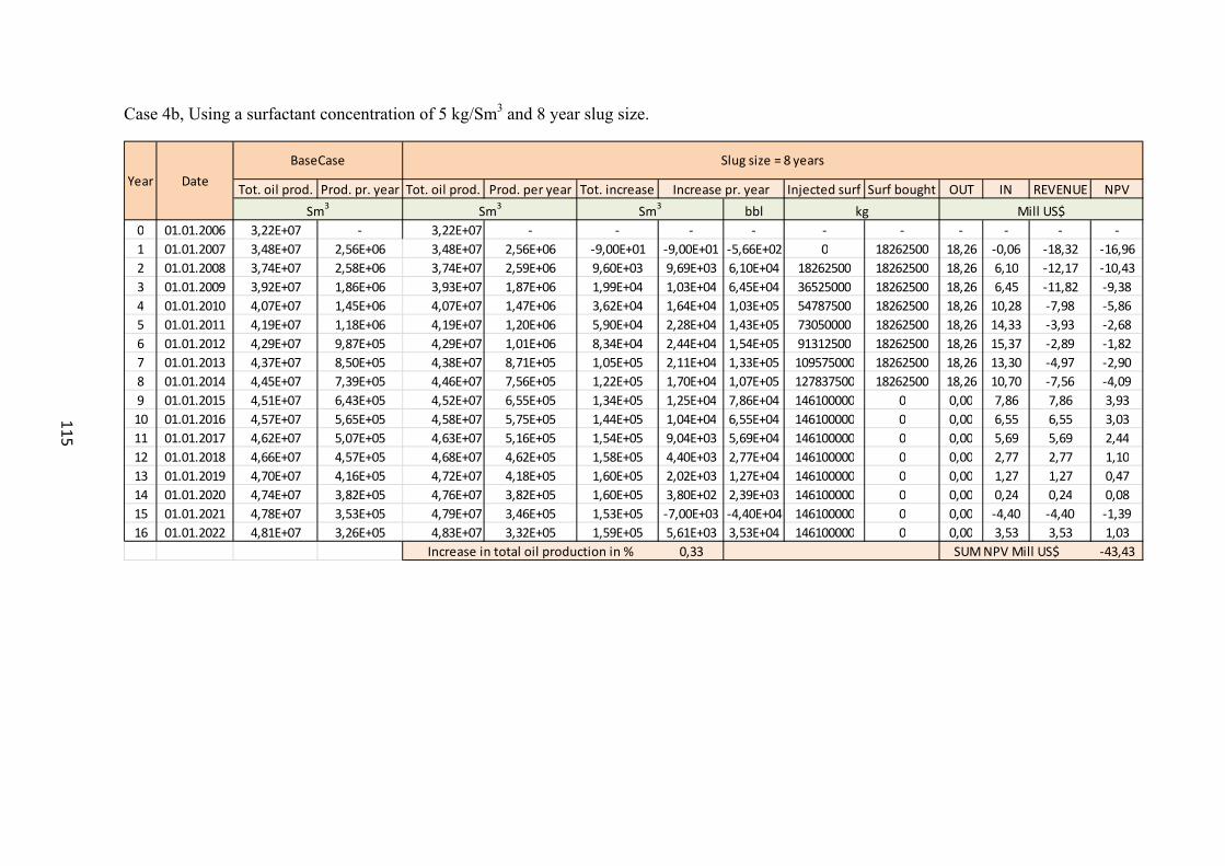
115
Case 4b, Using a surfactant concentration of 5 kg/Sm3 and 8 year slug size.
Tot. oil prod. Prod. pr. year Tot. oil prod. Prod. per year Tot. increase Injected surf Surf bought OUT IN REVENUE NPVbbl
0 01.01.2006 3,22E+07 - 3,22E+07 - - - - - - - - - -1 01.01.2007 3,48E+07 2,56E+06 3,48E+07 2,56E+06 -9,00E+01 -9,00E+01 -5,66E+02 0 18262500 18,26 -0,06 -18,32 -16,962 01.01.2008 3,74E+07 2,58E+06 3,74E+07 2,59E+06 9,60E+03 9,69E+03 6,10E+04 18262500 18262500 18,26 6,10 -12,17 -10,433 01.01.2009 3,92E+07 1,86E+06 3,93E+07 1,87E+06 1,99E+04 1,03E+04 6,45E+04 36525000 18262500 18,26 6,45 -11,82 -9,384 01.01.2010 4,07E+07 1,45E+06 4,07E+07 1,47E+06 3,62E+04 1,64E+04 1,03E+05 54787500 18262500 18,26 10,28 -7,98 -5,865 01.01.2011 4,19E+07 1,18E+06 4,19E+07 1,20E+06 5,90E+04 2,28E+04 1,43E+05 73050000 18262500 18,26 14,33 -3,93 -2,686 01.01.2012 4,29E+07 9,87E+05 4,29E+07 1,01E+06 8,34E+04 2,44E+04 1,54E+05 91312500 18262500 18,26 15,37 -2,89 -1,827 01.01.2013 4,37E+07 8,50E+05 4,38E+07 8,71E+05 1,05E+05 2,11E+04 1,33E+05 109575000 18262500 18,26 13,30 -4,97 -2,908 01.01.2014 4,45E+07 7,39E+05 4,46E+07 7,56E+05 1,22E+05 1,70E+04 1,07E+05 127837500 18262500 18,26 10,70 -7,56 -4,099 01.01.2015 4,51E+07 6,43E+05 4,52E+07 6,55E+05 1,34E+05 1,25E+04 7,86E+04 146100000 0 0,00 7,86 7,86 3,9310 01.01.2016 4,57E+07 5,65E+05 4,58E+07 5,75E+05 1,44E+05 1,04E+04 6,55E+04 146100000 0 0,00 6,55 6,55 3,0311 01.01.2017 4,62E+07 5,07E+05 4,63E+07 5,16E+05 1,54E+05 9,04E+03 5,69E+04 146100000 0 0,00 5,69 5,69 2,4412 01.01.2018 4,66E+07 4,57E+05 4,68E+07 4,62E+05 1,58E+05 4,40E+03 2,77E+04 146100000 0 0,00 2,77 2,77 1,1013 01.01.2019 4,70E+07 4,16E+05 4,72E+07 4,18E+05 1,60E+05 2,02E+03 1,27E+04 146100000 0 0,00 1,27 1,27 0,4714 01.01.2020 4,74E+07 3,82E+05 4,76E+07 3,82E+05 1,60E+05 3,80E+02 2,39E+03 146100000 0 0,00 0,24 0,24 0,0815 01.01.2021 4,78E+07 3,53E+05 4,79E+07 3,46E+05 1,53E+05 -7,00E+03 -4,40E+04 146100000 0 0,00 -4,40 -4,40 -1,3916 01.01.2022 4,81E+07 3,26E+05 4,83E+07 3,32E+05 1,59E+05 5,61E+03 3,53E+04 146100000 0 0,00 3,53 3,53 1,03
0,33 SUM NPV Mill US$ -43,43Increase in total oil production in %
Year DateBaseCase Slug size = 8 years
Increase pr. yearSm3 Sm3 Sm3 kg Mill US$

116

117
K. Adsorption
Incected surfactantskg kg %
Ile 7,31E+07 2,29E+07 31,4Tofte 7,31E+07 2,49E+07 34,1
Incected surfactantskg kg %
C-1H 5,48E+08 1,11E+08 20,2C-2H 5,48E+08 6,76E+07 12,3C-3H 5,48E+08 6,69E+07 12,2
All wells 1,64E+09 2,05E+08 12,5
Incected surfactantskg kg %
5 kg/Sm3 2,74E+08 6,76E+07 24,710 kg/Sm3 5,48E+08 8,08E+07 14,730 kg/Sm3 1,64E+09 1,01E+08 6,1
Incected surfactantskg kg %
2 years 7,31E+07 2,29E+07 31,45 years 9,60E+07 3,37E+07 35,18 years 1,30E+08 7,10E+07 54,8
Incected surfactantskg kg %
2 yeras 3,65E+07 1,22E+07 33,35 years 9,13E+07 3,13E+07 34,28 years 1,46E+08 4,42E+07 30,2
Case4a Adsorbtion
Case4b Adsorbtion
AdsorbtionCase1
Case2 Adsorbtion
Case3 Adsorbtion

118