evaluation of estimates of effort to develop … · evaluation of estimates of effort to develop...

EVALUATION OF ESTIMATES OF EFFORT TO DEVELOP APPLICATIONS WITH SUPERVISORY SYSTEM Renato Fernandez, [email protected] IFSP - Federal Institute of Education, Science and Technology of São Paulo São Paulo – Brasil

Valesca Alves Correa, valesca.correa @ unitau.com.br Luiz Eduardo Nunes Nicollini do Patrocínio, [email protected] UNITAU - University of Taubaté São Paulo – Brasil

The determination of the effort required to develop a project is the key factor in its approval and success. The effort includes not only the time and cost required for the development or maintenance of software projects, but also the number of people and hours required that each one must devote to the project. Efficient estimates allows the verification of the viability of the project, preparation of technical and commercial proposals, the production of detailed plans and schedules, and effective monitoring of the project. The risk measures have important roles in the development process of a project. Therefore, the estimates are the main activities of planning for the development of a software project. The Function Point Analysis (FPA) is a metric that allows a planning more realistic of the resource required. Based on a preliminary survey of the scope and structure of the application, FPA allows a reliable estimate, giving a preview of deadlines, costs and people needed for the development of the project. With the application of APF in automation process that involve supervisory systems, it will be possible for engineers to diagnose the necessary time and costs in the implementation of automated processes allowing for better planning. This study aims at applying the technique of algorithmic model of Function Point Analysis (FPA) to determine the effort required in developping supervisory systems using the LabVIEW application, where several parameters are applied to quantify the estimation of effort at various levels application mainly detecting the most complex elements that influence the project. As results we expected to get a major factor in measuring risk and still provide meaningful information to support decision that makes work more clear in terms of time, effort and cost, respecting their priorities.

Keywords: Function Point Analysis, Supervisory Systems, LabVIEW.

1. INTRODUCTION

In many industrial systems still exist equipment that should be fully automated, but for reasons of their own production dynamics are used manually. These situations cause the loss of productivity that is erroneously balanced by continuity or uninterrupted of the production process.

Software metrics are quantitative standards for measures of various aspects of a project or software product, and constitutes a powerful management tool, contributing to the elaboration of cost and time estimates more accurate and for the establishment of plausible targets, facilitating the process of decision and subsequent calculations of productivity and quality.

2. FUNCTION POINT ANALYSIS

The Function Point Analysis (FPA) is a technique for measuring the functionality provided by an application from the

user’s view. Function point is the unit of measure of this technique that aims to make the measurement independent of the technology used to build the application, ie, the FPA measure what the application does, not how it will be built (Vazques, Simões and Albert, 2010).

Therefore, the measurement process (also called count of function point) is based on a standardized assessment of the logical requirements of the user. This standard procedure is described by IFPUG (International Function Point Users Group) in its Counting Practices Manual.

The main techniques for estimating software development projects assume that the size of software is an important vector for determining the effort for its construction. Therefore, know the size is one of the first steps of the process of estimation of effort, time and cost.

Therefore, it is important to note that function points do not directly measure effort, productivity or cost. It is a measure of a functional size of software. This size, together with other variables, it might be used to derive productivity, to estimate effort and cost of the software project.

According to Andrade (2004), an application is a set of functions or business activities, which are divided into the following groups or types:

• Internal Logical File (ILF): Represent each logical grouping of data that can be part of a database or be a conventional file, whose maintenance is

performed by the application itself. The complexity of an internal logical file is calculated from the number of logical records referenced (a subgroup of

data elements, recognized by the user, within an internal logical file) and from the amount of referenced data (a field

ABCM Symposium Series in Mechatronics - Vol. 5 Copyright © 2012 by ABCM

Section II – Control Systems 15

mailto:[email protected]

mailto:[email protected]

recognized by the user, which is present in an internal logical file), using the counting rules and the definition of complexity.


Section II – Control Systems Page 116

• External Interface File (EIF): Represents each file referenced by the user used by the application, but resides outside the system boundary, ie the

maintenance is done from another application. The complexity of an external interface file is calculated from the number of logical records referenced (a subgroup of

data elements, recognized by the user, within an external interface file) and from the amount of referenced data (a field, recognized by the user, who is present in an external interface file), using the counting rules and the definition of complexity.

• External Input (EI): Represents each input coming directly from the user through a logical process only, with the aim of inserting,

modify or delete data from internal logical files. The complexity of an external input is calculated from the number of logical files referenced (an internal logical file or

an external interface read or maintained by a type of function) and from the amount of referenced data (a single field not recursive identified by the user, kept in an internal logical file for external input), using the counting rules and the definition of complexity.

• External Output (EO): Represent an elementary process that sends data or control information outside the boundary of the application. The

main objective is to present information to a user through a logical process and not just a simple data recovery. The processing logic must contain at least one mathematical formula or calculation, or create derived data. It can also be said that represent the application activities (processes) which results in the extraction of data from the application.

The complexity of an external output is calculated from the number of logical files referenced (a file read by the processing logic of the external output) and from the amount of referenced data (a field not recursive identified by the user, that appears in a external output), using the counting rules and the definition of complexity.

• External Inquiry (EI): Represent an elementary process that sends data or control information outside the boundary of the application. The

main objective is to present information to the user through the data recovery. The processing logic does not contains mathematical formulas or calculations, and does not create derived data. It can also be said that is an activity that, through an online requisition data generates an immediate response.

The complexity of an external inquiry is calculated from the number of logical files and the amount of referenced data (a field not recursive identified by the user, that appears in a external output).

Should be used only the most complex found between the pieces of input and output. The functions contribute to the calculation of Function Points based on quantity (number of functions) and

functional complexity assigned to each one. The number of FP (function points) of an application is determined into three phases of evaluation: • First Phase (Unadjusted Function Points):

Represent the specific and measurable functions of the business, provided to the user by application; • Second Phase (Adjustment Factor):

Represent the general functionality provided to the user by application; • Third Phase (Adjusted Function Points):

Represents the application of the Adjustment Factor over the calculated result in the first phase.

2.1. Unadjusted Function Points or Rough Function Points Calculation

A specific function of the user in an application is evaluated in terms of what is provided by the application and not as is provided. Only requested components and visible to the user are counted.

Each function, through its own criteria, should be classified according to their relative functional complexity, in Simple, Average or Complex.

For each function will be assigned a number of points according to their type and relative functional complexity (Andrade, 2004) as shown in “Tab. 1”.

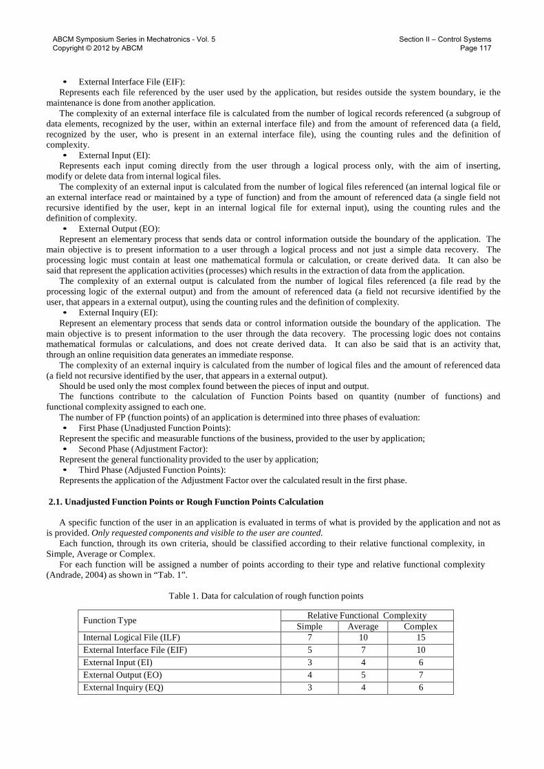
Table 1. Data for calculation of rough function points

Function Type Relative Functional Complexity Simple Average Complex

Internal Logical File (ILF) 7 10 15 External Interface File (EIF) 5 7 10 External Input (EI) 3 4 6 External Output (EO) 4 5 7 External Inquiry (EQ) 3 4 6



2.2 Calculation of Adjustment Factor According to Mecenas (2009), the value of the Adjustment Factor is calculated from 14 general characteristics of the

system, which allows a general evaluation of the application functionality. The general characteristics of a system are: • Data Communication: When resources are used for data communication to the sending or receiving data and

control information used by the application; • Distributed Processing: When the application predict the distribution of data or processing between multiple

CPUs installation; • Performance: This characteristics identifies the performance objectives of the application, established and

approved by the user, which have influenced (or will influence) the design, development, deployment and application support;

• Use of Equipment: Represents the need to make special considerations in systems architecture for the configuration of the equipment has not degradation;

• Transaction Volume: Measures the impact of the volume of transactions on application design; • Data Entry "online": Measures the volume of transactions are interactive data entry; • Efficiency of the End User: Examines the functions "online" designed and available to the end-user efficiency; • Update on-line ": Check the volume of internal logical files that have on-line maintenance and the impact of the

process of data recovery; • Complex Processing: Considers the impact on application design, caused by the type of processing complexity; • Code Reuse: Check if the application and its code were specifically engineered and designed to be reused in

other applications; • Facilities of Implementation: Considers the effort used to meet the requirements of data conversion to

application deployment; • Facility Operations: Check the application design and the requirements for startup, "backup” and recovery with the

objective of minimizing the manual operator intervention; • Multiple Locations: When the application is specifically designed and developed to be installed in multiple

locations or multiple organizations; • Facilities Change: When the application requirements predict the design and development of mechanisms to

facilitate operational changes, such as: capacity to issue reports generic, flexible queries or changes in the control data of the business (parameterization)

According to Hazan (2009), for each characteristic will be assigned a weight ranging from 0 (zero) to 5 (five),

according to the level of impact on the application, observing the criteria established for each characteristic, where: 0 (zero) : No influence, 1 (one): Minimal Influence, 2 (two): Moderate Influence, 3 (three): Average Influence, 4 (four): Significant Influence and five (5): Great Influence.

The level of general influence is obtained by summing the level of influence of each characteristic and the Adjustment Factor which is obtained by “Eq. (1)”.

Adjustment Factor = 0.65 + (Level of General Influence * 0.01) (1)

The adjustment factor is applied above the Rough Function Points (PFB) to allow the calculation of Adjusted Function Points (PFA). This value can range from 0.65 to 1.35, because the adjustment factor, when applied to the unadjusted function points, can produce a variation of plus or minus 35% and each point assigned to the level of influence affects the final result by 1%.

2.3 Calculating Adjusted Function Points

The Total Function Points (PFA) of the application will be found by multiplication of the number of Unadjusted

Function Points (PFB) by the Adjustment Factor (FA), according to the “Eq. (2)”.

PFA = PFB = x FA (2)

The process of estimating software projects involves four activities, and it is necessary to estimate the size of the product being developed, the effort to be employed for its implementation, the project duration and cost to the organization.

After analyzing the requirements to ensure product quality and size of software project, the next step is to calculate the

effort needed and then derive estimates of time and costs based on size estimates. Thus, by calculation the size of the project, it is possible to calculate all the other estimates, to identify the necessity of financial and personnel resources.



3. SUPERVISORY SYSTEM

The Supervisory Systems allow to monitor and to track the information from a production process or physical installation. The information are collected by data acquisition equipment and then manipulated, analyzed, stored and later presented to the user. These systems are also called SCADA (Supervisory Control and Data Acquisition).

Currently, industrial automation systems using communication and computing technologies to automate the monitoring and control of industrial processes, making data collection in complex environments, possibly geographically dispersed, and its presentation so friendly for the operator, with elaborate graphics resources (man- machine interface) and multimedia content.

The physical components of a system of supervision can be summarized in simplified form, in: sensors and actuators, communication network, remote stations (acquisition / control) and central monitoring system (computational system SCADA).

The process of control and data acquisition begins in the remote stations, PLC (Programmable Logic Controllers) and RTU (Remote Terminal Units), with the reading of the current values of the devices that are linked to it and their respective control. The PLC’s and RTU’s are specific computational units, used in manufacturing installation (or any other type of installation that you want to monitor) for the functionality to read input, perform calculations or controls, and update outputs. The difference between the PLC’s and RTU’s is that the PLC’s have more flexibility in programming language and control inputs and outputs, and the RTU’s have a more distributed architecture between the central processing unit and cards of input and output, with greater precision and sequencing of events.

The communication network is the platform through which information flow from PLC’s / RTU’s for SCADA system and taking into account the system requirements and distance to cover, can be implemented via Ethernet cables, fiber optics, dial-up lines, dedicated lines, radio modems, etc.

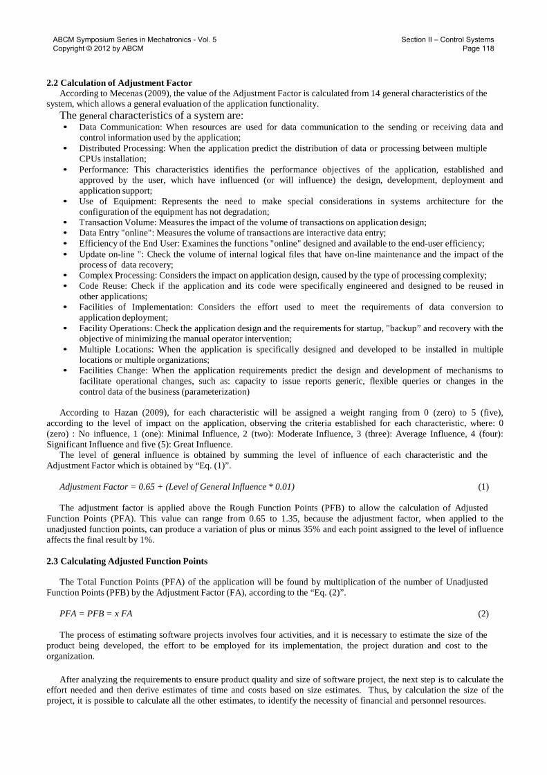
The central monitoring stations are the main units of SCADA systems, being responsible for collecting the information generated by remote stations and act in accordance with the detected events, which may be centralized on a single computer or distributed over a computer network, to enable sharing of information collected, according as “Fig 1”. (Daneels and Salter, 2000).

Figure 1. Supervision and Control System

4. SOFTWARE LABVIEW

The software LabVIEW is a application developed by National Instruments based in language G (graphical programming language or visual) that uses icons instead of text to create applications. This type of programming is based on the flow of data that define the execution of such data.

The LabVIEW allows creating test and measurement application, data acquisition, instrument control, data logging, measurement analysis and report generation, besides executable applications and shared libraries.

The programs in LabVIEW are called virtual instruments (VI - Virtual Instruments). The VI’s contain three main components: the front panel, block diagram and the panel of icons and connectors. The “Figure 2” shows a representation of the computing environment of LabVIEW software.



Figure 2. Front Panel and Block Diagram of LabVIEW software

The advantages of using this computing environment are summarized in the diversity of drivers and support for access to different peripherals/instruments and hardware, many library functions such as: Data Acquisition - data acquisition, analog and digital inputs and outputs; Signal Generation - periodic signal generation and other signals; Mathematics - mathematical functions and instructions; Statistics - statistics functions and instructions; Signal Conditioning ; Analisys (Velosa, 2009).

5. RESULTS

With he goal of using the APF methodology for estimating the size of a software, will be considered an application

shown by Lopes (2007), concerning the development of a Supervisory System using LabVIEW Software for Acquisition, Processing, Display of Signals and Storage Signals of a Power Mini System, which we evaluated the following interfaces: Simultaneous Measurements, Mini System State and Virtual Instrumentation, according as Block Diagram of “Fig 3”.

Figure 3. Block Diagram of Mini System

The inputs and outputs for the three interfaces evaluated will be analyzed in “Tab. 2, 3 and 4”:

Table 3. Identification of the components of input and output for Simultaneous Mini System State interface

Mini System State Inputs 4 keys Outputs 16 images to represent the states



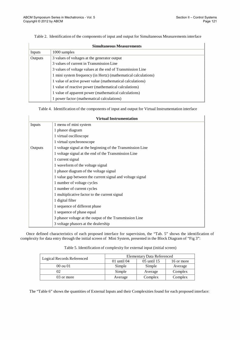
Table 2. Identification of the components of input and output for Simultaneous Measurements interface

Simultaneous Measurements Inputs 1000 samples Outputs 3 values of voltages at the generator output

3 values of current in Transmission Line 3 values of voltage values at the end of Transmission Line 1 mini system frequency (in Hertz) (mathematical calculations) 1 value of active power value (mathematical calculations) 1 value of reactive power (mathematical calculations) 1 value of apparent power (mathematical calculations) 1 power factor (mathematical calculations)

Table 4. Identification of the components of input and output for Virtual Instrumentation interface

Virtual Instrumentation Inputs 1 menu of mini system

1 phasor diagram 1 virtual oscilloscope 1 virtual synchronoscope

Outputs 1 voltage signal at the beginning of the Transmission Line 1 voltage signal at the end of the Transmission Line 1 current signal 1 waveform of the voltage signal 1 phasor diagram of the voltage signal 1 value gap between the current signal and voltage signal 1 number of voltage cycles 1 number of current cycles 1 multiplicative factor to the current signal 1 digital filter 1 sequence of different phase 1 sequence of phase equal 3 phasor voltage at the output of the Transmission Line 3 voltage phasors at the dealership

Once defined characteristics of each proposed interface for supervision, the “Tab. 5” shows the identification of complexity for data entry through the initial screen of Mini System, presented in the Block Diagram of “Fig 3”:

Table 5. Identification of complexity for external input (initial screen)

Logical Records Referenced Elementary Data Referenced 01 until 04 05 until 15 16 or more

00 ou 01 Simple Simple Average 02 Simple Average Complex 03 or more Average Complex Complex

The “Table 6” shows the quantities of External Inputs and their Complexities found for each proposed interface:




00 or 01 Simple Simple Average 02 or 03 Simple Average Complex

04 or more Average Complex Complex

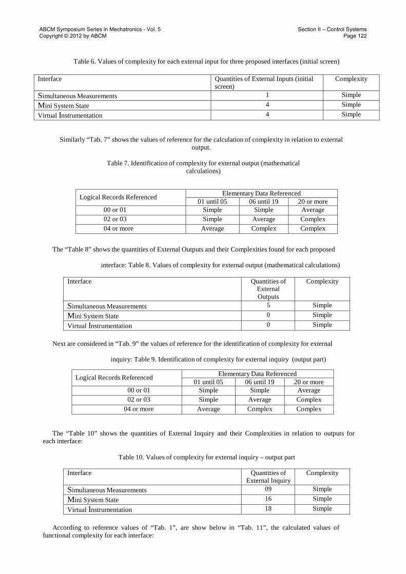
Table 6. Values of complexity for each external input for three proposed interfaces (initial screen)

Interface Quantities of External Inputs (initial screen)

Complexity

Simultaneous Measurements 1 Simple Mini System State 4 Simple Virtual Instrumentation 4 Simple

Similarly “Tab. 7” shows the values of reference for the calculation of complexity in relation to external output.

Table 7. Identification of complexity for external output (mathematical

calculations)


00 or 01 Simple Simple Average 02 or 03 Simple Average Complex 04 or more Average Complex Complex

The “Table 8” shows the quantities of External Outputs and their Complexities found for each proposed

interface: Table 8. Values of complexity for external output (mathematical calculations)

Interface Quantities of External Outputs

Complexity


Next are considered in “Tab. 9” the values of reference for the identification of complexity for external

inquiry: Table 9. Identification of complexity for external inquiry (output part)

The “Table 10” shows the quantities of External Inquiry and their Complexities in relation to outputs for each interface:

Table 10. Values of complexity for external inquiry – output part

Interface Quantities of

External Inquiry Complexity


According to reference values of “Tab. 1”, are show below in “Tab. 11”, the calculated values of

functional complexity for each interface:



Table 11. Values of Functional Complexity

Interface External Input External

Output External Inquiry

Realtive Functional Complexity

Simultaneous Measurements Simple / 3 Simple / 4 Simple / 3 10 Mini System State Simple / 3 Simple / 4 Simple / 3 10 Virtual Instrumentation Simple / 3 Simple / 4 Simple /3 10

Although there are 14 general characteristics of the system, as previously mentioned in item

Calculation of Adjustment Factor, Will be demonstrated Bellow in Table 12 the general characteristics inherent in the system of Acquisition, Processing, Display and Storage Signs of a Mini Power System and its respective levels of influence since the characteristics concerning Distributed Processing, Use of Equipment, Data Entry “On-Line”, Update “On-Line”, Code Reuse, Multiple Locations and Facilities of Change do not make part of the scope of the systems evaluated. The sum of degree of Influence of the characteristics, listed below, affect the effort required to develop the application.

As each characteristic can have a degree of influence varying from 0 to 5, the Total Degree of Influence (GIT) can vary from 0 to 70 (14 * 0 until 14 * 5).

Table 12. General characteristics of the system and

levels of influence

Characteristics Influence Level None [0] Minimum [1] Moderate [2] Average [3] Significant [4] Greate [5]

Data Communication 4 Performance 5 Transaction Volume 3 Efficiency of the end user 5 Complex Processing 3 Facilities of implementation 3 Facility operations 5 Total degree of influence (GIT) 28

The calculation of the Adjustment Factor (FAT) Will be obtained from the Total Degree of

Influence of the characteristics of application (GIT) using the “Eq. (3)”.

FAT = 1,35 + (0,01 * GIT) = 1,63 (3) As the since the adjustment factor, when applied to the unadjusted functions points, can produce a variation

about 35% and each point assigned to the level of influence affects the final resulting by 1%.

The adjustment factor is applied to the rough function points to allow the calculation of adjusted

function points. The “Table 13” shows the reference values for calculating the total of rough

function points:

Table 13. Level of complexity for calculation of the total rough function points

Complexity File Interface Input Output Query Simple 7 5 3 4 3 Average 10 7 4 5 4 Complex 15 10 6 7 6

Considering the weights shown in “Tab. 13”, the quantities of inputs shown in “Tab. 6”, the quantities



of output data shown in “Tab. 8” and the quantities of inquiry shown in “Tab. 10”, the rough function points are presented in “Tab. 14” for each interface evaluated.



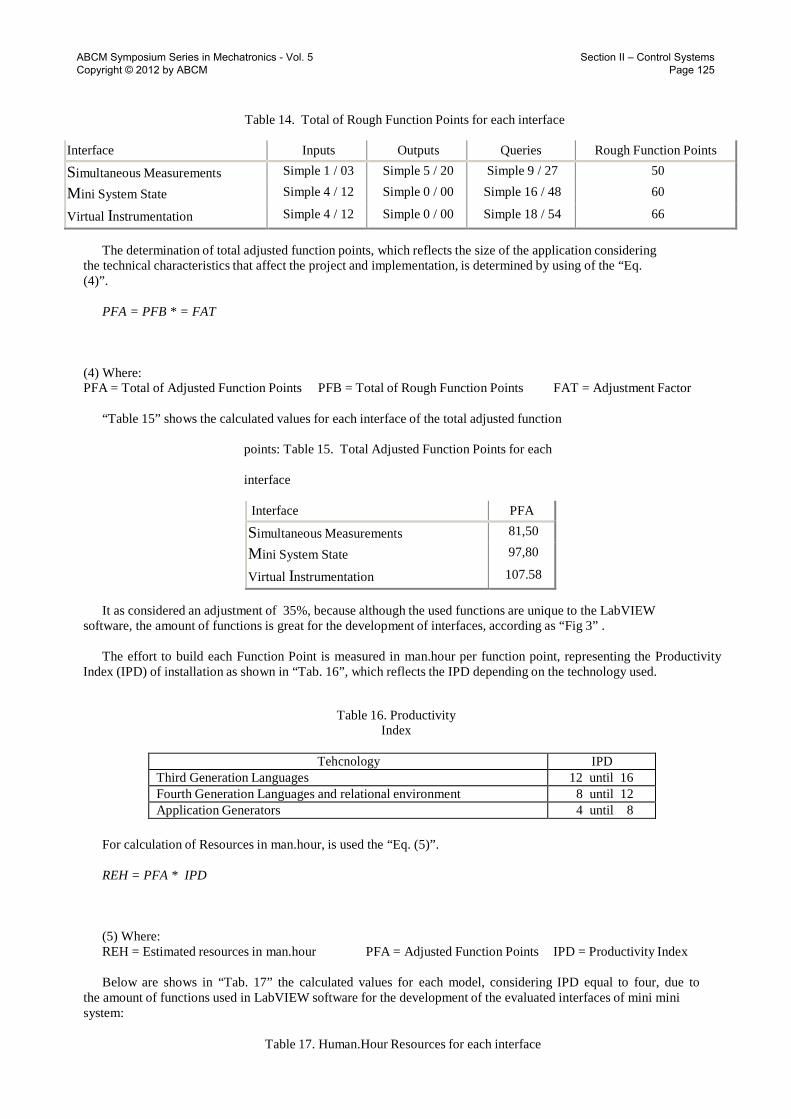
Table 14. Total of Rough Function Points for each interface

Interface Inputs Outputs Queries Rough Function Points

Simultaneous Measurements Simple 1 / 03 Simple 5 / 20 Simple 9 / 27 50

Mini System State Simple 4 / 12 Simple 0 / 00 Simple 16 / 48 60

Virtual Instrumentation Simple 4 / 12 Simple 0 / 00 Simple 18 / 54 66

The determination of total adjusted function points, which reflects the size of the application considering the technical characteristics that affect the project and implementation, is determined by using of the “Eq. (4)”.

PFA = PFB * = FAT

(4) Where: PFA = Total of Adjusted Function Points PFB = Total of Rough Function Points FAT = Adjustment Factor

“Table 15” shows the calculated values for each interface of the total adjusted function

points: Table 15. Total Adjusted Function Points for each

interface

Interface PFA

Simultaneous Measurements 81,50

Mini System State 97,80

Virtual Instrumentation 107.58

It as considered an adjustment of 35%, because although the used functions are unique to the LabVIEW software, the amount of functions is great for the development of interfaces, according as “Fig 3” .

The effort to build each Function Point is measured in man.hour per function point, representing the Productivity

Index (IPD) of installation as shown in “Tab. 16”, which reflects the IPD depending on the technology used.

Table 16. Productivity Index

Tehcnology IPD

Third Generation Languages 12 until 16 Fourth Generation Languages and relational environment 8 until 12 Application Generators 4 until 8

For calculation of Resources in man.hour, is used the “Eq. (5)”.

REH = PFA * IPD

(5) Where: REH = Estimated resources in man.hour PFA = Adjusted Function Points IPD = Productivity Index

Below are shows in “Tab. 17” the calculated values for each model, considering IPD equal to four, due to

the amount of functions used in LabVIEW software for the development of the evaluated interfaces of mini mini system:

Table 17. Human.Hour Resources for each interface



Interface REH Simultaneous Measurements 326,00 Mini System State 391,20 Virtual Instrumentation 430,32

For calculation of Estimated Resources in Human.Month the “Eq. (6)” is used.

REM = REH / 120 (6)


Section II – Control Systems 6

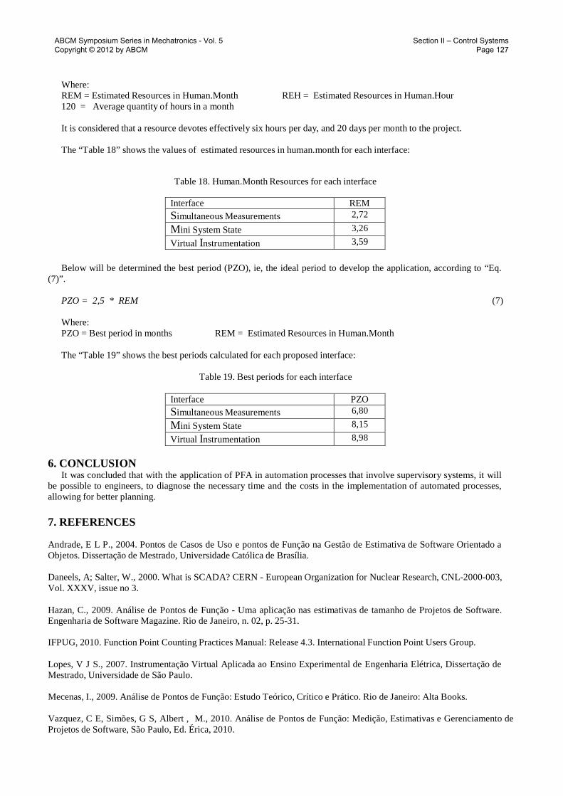
Where: REM = Estimated Resources in Human.Month REH = Estimated Resources in Human.Hour 120 = Average quantity of hours in a month

It is considered that a resource devotes effectively six hours per day, and 20 days per month to the project.

The “Table 18” shows the values of estimated resources in human.month for each interface:

Table 18. Human.Month Resources for each interface

Interface REM Simultaneous Measurements 2,72 Mini System State 3,26 Virtual Instrumentation 3,59

Below will be determined the best period (PZO), ie, the ideal period to develop the application, according to “Eq.

(7)”.

PZO = 2,5 * REM (7)

Where: PZO = Best period in months REM = Estimated Resources in Human.Month

The “Table 19” shows the best periods calculated for each proposed interface:

Table 19. Best periods for each interface

Interface PZO Simultaneous Measurements 6,80 Mini System State 8,15 Virtual Instrumentation 8,98

6. CONCLUSION

It was concluded that with the application of PFA in automation processes that involve supervisory systems, it will be possible to engineers, to diagnose the necessary time and the costs in the implementation of automated processes, allowing for better planning.

7. REFERENCES

Andrade, E L P., 2004. Pontos de Casos de Uso e pontos de Função na Gestão de Estimativa de Software Orientado a Objetos. Dissertação de Mestrado, Universidade Católica de Brasília.

Daneels, A; Salter, W., 2000. What is SCADA? CERN - European Organization for Nuclear Research, CNL-2000-003, Vol. XXXV, issue no 3.

Hazan, C., 2009. Análise de Pontos de Função - Uma aplicação nas estimativas de tamanho de Projetos de Software. Engenharia de Software Magazine. Rio de Janeiro, n. 02, p. 25-31.

IFPUG, 2010. Function Point Counting Practices Manual: Release 4.3. International Function Point Users Group.

Lopes, V J S., 2007. Instrumentação Virtual Aplicada ao Ensino Experimental de Engenharia Elétrica, Dissertação de Mestrado, Universidade de São Paulo.

Mecenas, I., 2009. Análise de Pontos de Função: Estudo Teórico, Crítico e Prático. Rio de Janeiro: Alta Books.

Vazquez, C E, Simões, G S, Albert , M., 2010. Análise de Pontos de Função: Medição, Estimativas e Gerenciamento de Projetos de Software, São Paulo, Ed. Érica, 2010.



Velosa, J E C., 2009. Controlo Automático de um Interferómetro para Monitorização e Caracterização de Sensores Interferómetricos. Dissertação de Mestrado, Universidade da Madeira, Portugal.



evaluation of estimates of effort to develop … · evaluation of estimates of effort to develop...

Documents