evaluation of engineering stresses as the “correct” measure of “physical” stresses in large...

International Journal of Engineering Inventions

e-ISSN: 2278-7461, p-ISSN: 2319-6491

Volume 2, Issue 8 (May 2013) PP: 16-27

www.ijeijournal.com Page | 16

Evaluation of Engineering Stresses as the “Correct” Measure of

“Physical” Stresses in Large Strain Geometrically Nonlinear

Problems

A. E. Mohmed1, N. M. Akasha

2, F. M. Adam

3

1Dept. of Civil Engineering, Sudan University of Science and Technology, Sudan

2Dept. of Civil Engineering, Sudan University of Science and Technology, Sudan

3Dept. of Civil Engineering, Jazan University, Kingdom of Saudi Arabia

Abstract: In this paper, Lagrangian formulations for geometric nonlinear plane stress/strain problems based on

different stress measures are evaluated. A Total Lagrangian formulation based on the exact Engineering strains

is developed. The 2ndPiola-Kirchhoff stresses based on the well known Green strains and the Engineering

stresses based on the exact Engineering (geometric or conventional) strains obtained from Total Lagrangian

formulations are compared with the true Cauchy stresses. The Engineering stresses based on the assumption of

small shear strains are also compared with the above mentioned stresses. Geometric nonlinear Total

Lagrangian formulations applied on two-dimensional elasticity using 4-node plane finite elements were used.

The formulations were implemented into the finite element program (NUSAP). The solution of nonlinear

equations was obtained by the Newton-Raphson method. The program was applied to obtain stresses for the

different strain measures. The true Cauchy stresses were obtained by using the Logarithmic strains. The

evaluation was based on comparing the results of three numerical examples. For moderate and large strains,

the exact Engineering stresses are good measures of the correct physical stresses. Thus, these must be used

when the stresses are required from a Total Lagrangian solution.

Keywords: Cauchy stresses, Engineering strain, Geometric Nonlinear, Plain stress/strain, Total Lagrangian

I. INTRODUCTION Almost all structures behave in some nonlinear manner prior to reaching their limit of resistance. For

this reason, most modern codes have incorporated certain provisions to consider nonlinear effects e.g. limit state

design methods. Also, the use of light, high strength materials, resulting in light “tall” structures, introduces

certain degrees of nonlinearity. This coupled with advance in solution methods and computing facilities make

room for geometric nonlinear analysis. The major problem in geometrically nonlinear (GNL) finite element

analysis is the need to define reference coordinates and to specify the relevant stress and strain measures.

The two main finite element formulations for GNL problems are the Eulerian formulations (EFMS)

and the Lagrangian formulations (LFMS). As stated, among others, by Yang and Kuo [1], Crisfield [2],

Zeinkiewicz and Taylor [3] and Mohamed [4] LFMS, in contrast to EFMS, are suitable in solid mechanics

applications. This is mainly due to the ease with which they handle complicated boundaries and their ability to

follow material points enabling the accurate treatment of history dependent materials. There are two main

approaches to LFMS, namely the Total Lagrangian (TL) and the Updated Lagrangian (UL). Yang and Kuo [1],

Zeinkiewicz and Taylor [3], Belytschko [5] and Marinkowic et al [6], stated that the UL approach provides the

most efficient formulation and can be considered equivalent to the EFM. Wood and Zeinkiewicz [7] stated that

the TL approach offers advantages since the initial configuration remains constant which simplifies formulation

and computation. Surana and Sorem [8] presented a TL approach for framed structures with no restrictions on

rotation increments. Djermane et al [9] pointed out that the TL formulation is now recognized as the most

realistic civil engineering approach. But, the main serious drawback of the TL approach is that it is based on the

Green strains, which are unsuitable for work with large strains. Also, the 2nd

Piola-Kirchhoff stresses, which are

work conjugate to the Green strains, are defined in the deformed configuration and should be transformed to the

undeformed configuration [1], [2], [3], [4] and [8]. Thus, the TL approach while being very well established,

having the above mentioned advantages and giving accurate displacement values, will result in stresses with no

physical significance [2].

As for the definition of stress and strain measures, Crisfield [2] and Bonet and Wood [10] proposed the

use, as work conjugate in the virtual work expression, the Green strains with the 2nd

Piola-Kirchhoff stresses, the

Engineering (conventional or geometric) strains with the Engineering stresses and the Logarithmic strains with

the Cauchy "true" stresses. Yang and Kuo [1] used, as work conjugate, the Green-Lagrange strains with the

2nd

Piola-Kirchhoff stresses, the Infinitesimal strains with the Cauchy stresses and the Updated Green strains

with the Updated Kirchhoff stresses. They adopted the Updated Kirchhoff stresses as the measure of the "true"

Evaluation of Engineering Stresses as the “Correct” Measure of “Physical” Stresses in Large Strain


physical stresses. In fact, the proposition that: using the UL approach converts the 2nd

Piola-Kirchhoff stresses to

the "true" stresses is also adopted by many researchers [2], [3], [5], [6] and [10].

An alternative TL approach that results in evaluating "correct" stresses was developed by Surana and

Sorem [8]. Their formulation for framed structures removed the restrictions of small rotation increments by

retaining nonlinear terms in the definition of the element displacement field. Mohamed [4] presented a TL

formulation based on the Engineering strains which resulted in the correct stresses for small strain large rotation

deformation of beams. Mohamed and Adam [11], [12] extended the TL formulation based on Engineering

strains to the analysis of shell structures. Akasha [13] and Akasha and Mohamed [14], [15] developed a similar

TL formulation for plane stress/strain problems. These formulations were based on using the Engineering strains

with the Engineering stresses in the virtual work expression. The formulations were developed basing the

variation of the Engineering strains on the variation of Green strains. These formulations are similar to the

positional formulation based on Engineering strains used by Greco and Ferreira [16]. The formulations were,

also, extended to include the evaluation of the true Cauchy stresses based on Logarithmic strains [13], [14] and

[17]. The only limitation of these formulations is the assumption that the shear strains are small. However, it is

possible to avoid this limitation by considering the exact variation of the Engineering strains.

This paper presents a TL formulation based the exact variation of Engineering strains. The paper is,

also take an evaluation of the TL nonlinear stresses which are compared with the true Cauchy stresses presented

by Akasha and Mohamed [17] using the Logarithmic strains. The comparison is carried out for plane

stress/strain problems with the intention of investigating the effect of large strains on the different stress

measures. The effect of avoiding the limitation on shear strains is, also, looked into. The comparison is

considered as a criterion for ensuring the accuracy, consistency and convergence to the correct results of the

nonlinear analysis. Thus, the aim of the evaluation is pointing out when the TL formulation based on

Engineering strains is to be used, with confidence, in the analysis of large strain problems.

II. NONLINEAR FINITE ELEMENT FORMULATION In the following sections there are two alternative Lagrangian formulations of the incremental

equilibrium equations for large strain two dimensional problems which are outlined below.

2.1 Geometrically Non-linear Finite Element TL Formulation based on Green strains (TLG): The 2

ndPiola-Kirchhoff stresses, work conjugate to the Green-Lagrange strains, are the internal forces

per unit initial area acting along the normal and tangential directions at the deformed configuration [1], [2] and

[4]. Thus, these stresses are referred to the convected coordinates in the deformed configuration but measured

per unit area of the undeformed body with attempts to take this into consideration in the virtual work expression

result in an unsymmetrical stiffness matrix [4]. Hence, direct proportionality between the 2nd

Piola-Kirchhoff

stresses, s0, and the Green-Lagrange strains, e0, is assumed when writing the virtual work expression. In two

dimensions, with reference to the initial configuration (t=0), the Green strains are given by:

𝒆𝟎 = 𝑒𝑥 ,𝑒𝒚,𝑒𝑥𝑦 𝑇

= 1

2 𝐅T𝐅 − 𝐈 (1)

where F is the displacement gradient matrix.

In a finite element formulation equation (1) is written as:

𝒆𝟎 = 𝒆0𝟎 + 𝒆0

𝑳 = 𝑩𝟎𝒂𝟎 +1

2𝑩𝑳 𝒂𝟎 𝒂0 (2)

where 𝒂𝟎 is the vector of nodal variables.

The nonlinear strain e0Lcan be written as:

𝒆𝟎𝑳 =

1

2𝑩𝑳 𝒂𝟎 𝒂0 =

1

2𝑨𝜃𝑮0𝒂0 (3)

The strain displacement matrix B is given by:

𝑩 = 𝑩𝟎 + 𝑩𝑳 𝒂𝟎 (4) The tangent stiffness matrix now takes the form:

𝑲𝑇 = 𝑲0 + 𝑲𝐿 𝒂𝟎 + 𝑲𝜎 (5)

where:

𝑲0 + 𝑲𝐿 𝒂𝟎 = 𝑩𝑇𝑫𝑩 𝑑𝑉0𝑉0

(6)𝑎

in which D is the modulus matrix, and the initial stress stiffness matrix is given by:

𝑲𝜎 = 𝑮0𝑇𝑷0𝑖𝑮0𝑑𝑉0

𝑉0

(6)𝑏

in which 𝑷0𝑖 is the initial stress matrix.

The displacement increments ∆a0i are evaluated by using KT and the residuals as:



∆𝒂0𝑖 = − 𝑲𝑇

−1𝝋𝑖 (7)

The total displacements are, then, obtained as:

a0i+1 = a0

i + ∆a0i (8)

The strain increments are defined by:

∆𝒆𝑜𝑖 = 𝑩𝟎 + 𝑩𝑳 𝒂0

𝑖 + 1

2𝑩𝑳 ∆𝒂0

𝑖 ∆𝒂0𝑖 (9)

And the stress increments are given by:

∆𝒔𝟎𝒊 = 𝑫∆𝒆𝑜

𝑖 (10)

And the total stresses are:

𝒔𝟎𝒊+𝟏 = 𝒔0

𝒊 + ∆𝒔𝟎𝒊 (11)

From which the nodal residual forces are evaluated as follows:

−𝝋𝒊+𝟏 = 𝑹 − 𝑩𝑇𝒔𝟎𝒊+𝟏𝑑𝑉0

𝑉0

(12)

where 𝑹 is the vector of applied equivalent nodal forces and:

𝑩 = 𝑩𝟎 + 𝑩𝑳 𝒂0𝒊+𝟏

2.2 Geometrically Non-linear Finite Element TL Formulation based on Engineering strains (TLE):

In two dimensions the geometric strains, unit stretches, εx and εy are defined by the change in length

per unit initial length of line elements originally oriented parallel to the x and y axes respectively. The shear

strain γxy

is the actual angle change.

The geometric strains, as defined above, are given in terms of Green strains by:

휀𝑥 = 𝑔𝑥 .𝑔𝑥 1

2 − 1 = 1 + 2𝑒𝑥 1

2 − 1

휀𝑦 = 𝑔𝑦 .𝑔𝑦 1

2 − 1 = 1 + 2𝑒𝑦 1

2 − 1 (13)

And the shear strain is defined as:

𝛾𝑥𝑦 = sin−1𝑒𝑥𝑦

1 + 2𝑒𝑥 1

2 1 + 2𝑒𝑦 1

2

(14)

where:

𝑒𝑥𝑦 = 𝑔𝑥 .𝑔𝑦 = 1 + 2𝑒𝑥 1

2 1 + 2𝑒𝑦 1

2 sin 𝛾𝑥𝑦

𝑔𝑥 = 𝜕𝑅

𝜕𝑥 , 𝑔𝑦 =

𝜕𝑅

𝜕𝑦 are the displacement gradient vectors, and R is the position vector after

deformation.

The variation in the Engineering strains is given by:

𝛿𝜺0 = 𝑯 𝛿𝒆0 (15) where:

𝛿𝒆0 = 𝑩0 + 𝑩𝐿 𝒂0 𝛿𝒂0 = 𝑩0 + 𝑨𝜃𝑮0 𝛿𝒂0 = 𝑩𝛿𝒂0 (16)

From which, the variations in the Engineering strains are given by:

𝛿𝜺0 = 𝑯𝑩𝛿𝒂0 = 𝑩∗ 𝛿𝒂0 (17)

In which B is the strain matrix, and H relates variation in Engineering strains to variation in Green

strains.

The incremental equilibrium equations in terms of Engineering stresses are:

𝑲𝑇∗ ∆𝒂0 = 𝑹 − 𝑩𝑇𝑯𝑇𝝈 𝑑𝑉0

𝑉0

= 𝑹 − 𝑩∗𝑇𝝈 𝑑𝑉0𝑉0

(18)

where 𝝈 are the Engineering stresses.

The tangent stiffness matrix 𝑲𝑇∗ is now given by:

𝑲𝑇∗ = 𝑲0

∗ + 𝑲𝐿∗ + 𝑲𝜎

∗ + 𝑲𝜎∗∗ (19)

where:

𝑲0∗ = 𝑩0

𝑇𝑯𝑇𝑫𝑯𝑩0𝑑𝑉0𝑉0

20 𝑎

and

𝑲𝐿∗ = 𝑩0

𝑇𝑯𝑇𝑫𝑯𝑩𝐿𝑑𝑉0𝑉0

+ 𝑩𝐿𝑇𝑯𝑇𝑫𝑯𝑩0𝑑𝑉0

𝑉0

+ 𝑩𝐿𝑇𝑯𝑇𝑫𝑯𝑩𝐿𝑑𝑉0

𝑉0

20 𝑏

and 𝑲𝜎∗ is the symmetric matrix dependent on the Engineering stress, and can be written as:



𝑲𝜎∗ = 𝑮0

𝑇𝑷𝟎𝒊∗ 𝑮0𝑑𝑉0

𝑉0

(21)

where 𝑮0 is a matrix containing shape function derivatives.

and the initial stress matrix 𝑷𝟎𝒊∗ is defined as:

𝑷𝟎𝒊∗ =

𝜎𝒙∗ 𝐼 𝜎𝒙𝒚

∗ 𝐼

𝜎𝒙𝒚∗ 𝐼 𝜎𝒚

∗ 𝐼 (22)

where 𝐼 is 22 unit matrix.

and 𝝈∗is the stress vector given by:

𝝈∗ =

𝜎𝒙∗

𝜎𝒚∗

𝜎𝒙𝒚∗ = 𝑯𝑇

𝜎𝒙𝜎𝒚𝜎𝒙𝒚

(23)

and the additional geometric stiffness matrix 𝑲𝜎∗∗ takes the following form:

𝑲𝜎∗∗ = 𝑩𝑇𝑷𝟎𝒊

∗∗𝑩 𝑑𝑉0𝑉0

(24)

where 𝑷𝟎𝒊∗∗ is obtained from:

𝛿𝑯𝑇𝝈 = 𝑷𝟎𝒊∗∗𝛿𝜺0 = 𝑷𝟎𝒊

∗∗ 𝑩𝛿𝒂0 (25)

Upon solving the incremental equilibrium equations for the displacement increments ∆a0i and evaluating

the total displacements a incremental strains are obtained as:

∆𝜺0𝑖 = 𝑯 𝐁𝟎 + 𝐁𝑳 𝒂0

𝑖 + 1

2𝐁𝑳 ∆𝒂0

𝑖 ∆𝒂0𝑖 (26)

The stress increments are then given by:

∆𝝈0𝑖 = 𝑫∆𝜺0

𝑖 (27) And the total stresses are:

𝝈0𝑖+1 = 𝝈0

𝑖 + ∆𝝈0𝑖 (28)

The residual forces, for a new displacement increment, are then equal to:

−𝝋𝒊+𝟏 = 𝐑 − 𝑩𝑇𝑯𝑇𝝈𝟎𝒊+𝟏𝑑𝑉0

𝑉0

= 𝐑 − 𝑩∗𝑇𝝈𝟎𝒊+𝟏𝑑𝑉0

𝑉0

(29)

III. NUMERICAL RESULTS ANDDISCUSSION The finite element TLG and TLE formulations described in the above section were implemented in the

NUSAP coded by FORTRAN. Three numerical examples of large deformation problems were examined to

demonstrate the degree of accuracy that can be obtained by using the geometrically non-linear formulations based

on 4-node isoparametric plane stress/strain elements. The examples were also solved by using Green strains and

the approximate Engineering strains [15]. The results of the stresses of the three TL formulations are compared

with the true Cauchy stresses based on Logarithmic strains obtained using the formulation presented in references

[13] and [17].

3.1 Cantilever under point load at free end: The TLE (Eng Exact), approximate TLE (Eng) and TLG (Green) formulations were tested by

analyzing the cantilever plate with vertical load at the free end. The cantilever is of dimensions L=2.5 m, D = 1

m and t = 0.1 m as shown in Figure (1). The numerical values of material property parameters are; Young's

modulus, E = 2x108 kN/m

2 and Poisson’s ratio υ = 0.3. The structure is modeled with 40 equal size

isoparametric elements. The cantilever was, also, analyzed using Logarithmic (Log) strains for comparison.

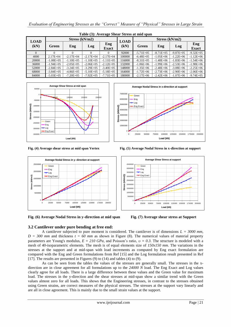
Graphical comparison of results of the stresses at the support and at mid- span are presented in Figures

(2) to (7). Tables (1), (2) and (3) show the stresses at mid-span. The results of the true Cauchy stresses are also

shown. At mid-span the results for the direct stresses are almost identical for the Log and Eng exact

formulations. The slight differences may be attributed to the large strain value at mid-span. The Green values

vary greatly from the correct values and are almost zero in the x-direction for maximum load. The differences in

the shear stress values are mainly due to the assumption that the shear strain is small in the formulations other

than Eng Exact. The results for the direct stresses at the support are in close agreement. Those for the shear

stresses at the support are in close agreement for Eng Exact and Log formulations. The shear values from the

Eng formulation are approximate. The shear values from the Green formulation differ largely from the correct

values as expected.



Fig. (1) Cantilever plate with vertical load at free end

Table (1): Average Nodal Stress in x-direction at mid span

LOAD

(kN)

Stress (kN/m2)

LOAD

(kN)

Stress (kN/m2)

Green Eng Log Eng

Exact Green Eng Log

Eng

Exact 0 0 0 0 0 92000 -5.64E+06 -5.84E+06 -6.63E+06 -4.86E+06

4000 -2.99E+05 -2.99E+05 -2.99E+05 -2.99E+05 100000 -5.82E+06 -5.83E+06 -6.65E+06 -4.51E+06

20000 -1.48E+06 -1.50E+06 -1.51E+06 -1.49E+06 116000 -5.89E+06 -5.09E+06 -5.70E+06 -2.82E+06

36000 -2.62E+06 -2.71E+06 -2.80E+06 -2.66E+06 132000 -5.47E+06 -3.03E+06 -2.79E+06 6.57E+05

52000 -3.69E+06 -3.89E+06 -4.14E+06 -3.75E+06 148000 -4.42E+06 8.10E+05 2.94E+06 6.54E+06

68000 -4.63E+06 -4.94E+06 -5.41E+06 -4.59E+06 164000 -2.62E+06 6.94E+06 1.24E+07 1.55E+07

84000 -5.37E+06 -5.67E+06 -6.38E+06 -4.95E+06 180000 8.12E+04 1.58E+07 2.63E+07 2.81E+07

Fig. (2): Average Nodal Stress in x-direction at mid span Fig. (3): Average Nodal Stress in y-direction at mid span

Table (2): Average Nodal Stress in y-direction at mid span

LOA

D

(kN)

Stress (kN/m2)

LOAD

(kN)

Stress (kN/m2)

Green Eng Log Eng

Exact Green Eng Log

Eng

Exact 0 0 0 0 0 92000 3.74E+05 9.81E+05 1.01E+06 1.99E+06

4000 2.42E+04 2.44E+04 2.44E+04 2.43E+04 100000 6.92E+05 1.68E+06 1.90E+06 3.02E+06

20000 1.20E+05 1.28E+05 1.38E+05 1.20E+05 116000 1.63E+06 3.81E+06 4.82E+06 6.08E+06

36000 1.98E+05 2.27E+05 2.77E+05 1.77E+05 132000 3.08E+06 7.24E+06 9.81E+06 1.09E+07

52000 2.22E+05 2.53E+05 3.65E+05 9.64E+04 148000 5.18E+06 1.24E+07 1.76E+07 1.80E+07

68000 1.35E+05 7.97E+04 2.34E+05 2.89E+05 164000 8.06E+06 1.96E+07 2.88E+07 2.79E+07

84000 1.39E+05 4.81E+05 3.91E+05 1.22E+06 180000 1.19E+07 2.93E+07 4.42E+07 4.11E+07

Average Nodal Stress in y-direction at mid span

-5000000

0

5000000

10000000

15000000

20000000

25000000

30000000

35000000

40000000

45000000

50000000

0 25000 50000 75000 100000 125000 150000 175000 200000

Load (kN)

Str

ess (

kN

/m2)

Green

Eng

Log

Eng Exact

L = 2.5 m

y P/2

x D = 1 m

P/2

Average Nodal Stress in x-direction at mid span

-10000000

-5000000

0

5000000

10000000

15000000

20000000

25000000

30000000

0 25000 50000 75000 100000 125000 150000 175000 200000

Load (kN)

Str

ess (

kN

/m2)

Green

Eng

Log

Eng Exact



Table (3): Average Shear Stress at mid span

LOAD

(kN)

Stress (kN/m2) LOAD

(kN)

Stress (kN/m2)

Green Eng Log Eng

Exact Green Eng Log

Eng

Exact 0 0 0 0 0 92000 -5.71E+05 -8.71E+05 -9.87E+05 -9.32E+05

4000 2.17E+04 -2.17E+04 -2.17E+04 -2.17E+04 100000 -6.48E+05 -1.05E+06 -1.22E+06 -1.12E+06

20000 -1.08E+05 -1.10E+05 -1.10E+05 -1.11E+05 116000 -8.31E+05 -1.48E+06 -1.83E+06 -1.54E+06

36000 -1.94E+05 -2.05E+05 -2.06E+05 -2.12E+05 132000 -1.06E+06 -1.99E+06 -2.53E+06 -1.98E+06

52000 -2.84E+05 -3.24E+05 -3.29E+05 -3.40E+05 148000 -1.35E+06 -2.48E+06 -3.08E+06 -2.25E+06

68000 -3.84E+05 -4.86E+05 -5.10E+05 -5.18E+05 164000 -1.72E+06 -2.73E+06 -2.90E+06 -2.06E+06

84000 -5.03E+05 -7.20E+05 -7.92E+05 -7.71E+05 180000 -2.17E+06 -2.42E+06 -1.07E+06 -9.74E+05

Fig. (4) Average shear stress at mid span Vertex Fig. (5) Average Nodal Stress in x-direction at support

Fig. (6) Average Nodal Stress in y-direction at mid span Fig. (7) Average shear stress at Support

3.2 Cantilever under pure bending at free end:

A cantilever subjected to pure moment is considered. The cantilever is of dimensions L = 3000 mm,

D = 300 mm and thickness t = 60 mm as shown in Figure (8). The numerical values of material property

parameters are Young's modulus, E = 210 GPa, and Poisson’s ratio, = 0.3. The structure is modeled with a

mesh of 40-isoparametric elements. The mesh is of equal elements size of 150x150 mm. The variations in the

stresses at the support and at mid-span with load increments as computed by Eng exact formulation are

compared with the Eng and Green formulations from Ref [15] and the Log formulation result presented in Ref

[17]. The results are presented in Figures (9) to (14) and tables (4) to (9).

As can be seen from the tables the values of the stresses are generally small. The stresses in the x-

direction are in close agreement for all formulations up to the 24000 N load. The Eng Exact and Log values

clearly agree for all loads. There is a large difference between these values and the Green value for maximum

load. The stresses in the y-direction and the shear stresses at mid-span show a similar trend with the Green

values almost zero for all loads. This shows that the Engineering stresses, in contrast to the stresses obtained

using Green strains, are correct measures of the physical stresses. The stresses at the support vary linearly and

are all in close agreement. This is mainly due to the small strain values at the support.

Average Nodal Stress in x-direction at support

0

10000000

20000000

30000000

40000000

50000000

60000000

70000000

0 25000 50000 75000 100000 125000 150000 175000 200000

Load (kN)

Str

ess (

kN

/m2)

Green

Eng

Log

Eng Exact

Average Shear Stress at support

0

5000000

10000000

15000000

20000000

25000000

30000000

35000000

40000000

45000000

0 25000 50000 75000 100000 125000 150000 175000 200000

Load (kN)

Str

ess (

kN

/m2))

Green

Eng

Log

Eng Exact

Average Shear Stress at mid span

-3500000

-3000000

-2500000

-2000000

-1500000

-1000000

-500000

0

500000

0 50000 100000 150000 200000

Load (kN)

Str

ess (

kN

/m2)

Green

Eng.

Log

Eng Exact

Average Nodal Stress in y- direction at support

0

5000000

10000000

15000000

20000000

25000000

0 25000 50000 75000 100000 125000 150000 175000 200000

Load (kN)

Str

ess (

kN

/m2)

Green

Eng

Log

Eng Exact



Figure 8: Cantilever under pure bending


Stress (N/mm2) LOAD

(N) Eng Exact Eng (Geom) Green Log

0 0 0 0 0

1.23E+00 1.24E+00 1.22E+00 1.24E+00 6000

2.43E+00 2.47E+00 2.41E+00 2.50E+00 12000

3.37E+00 3.54E+00 3.49E+00 3.58E+00 18000

3.63E+00 4.09E+00 4.35E+00 3.94E+00 24000

2.61E+00 3.58E+00 4.84E+00 2.71E+00 30000

Fig. (9): Average Nodal Stress in x-direction at mid span Fig. (10): Average Nodal Stress in y-direction at mid span


Stress (N/mm2) LOAD


0 0 0 0 0

9.13E-02 9.59E-02 9.75E-02 9.62E-02 6000

7.57E-02 1.21E-01 1.66E-01 1.05E-01 12000

3.18E-01 1.50E-01 1.33E-01 2.86E-01 18000

1.54E+00 1.10E+00 1.15E-01 1.67E+00 24000

4.18E+00 3.26E+00 7.18E-01 4.92E+00 30000

Table (6): Average Shear Stress at mid span Stress (N/mm

2) LOAD


0 0 0 0 0

2.67E-03 1.26E-03 6.77E-04 4.47E-05 6000

2.23E-02 1.48E-02 5.56E-03 1.50E-02 12000

8.97E-02 6.87E-02 2.32E-02 8.82E-02 18000

2.48E-01 2.02E-01 6.56E-02 2.83E-01 24000

5.40E-01 4.43E-01 1.47E-01 6.39E-01 30000


-1

0

1

2

3

4

5

6

0 5000 10000 15000 20000 25000 30000 35000

Load (N)

Str

ess (

N/m

m2)

Eng Exac

Geom

Green

Log

L = 3 m

P

P

x

y

D = 0.3 m


0

1

2

3

4

5

6

0 5000 10000 15000 20000 25000 30000 35000

Load (N)

Str

ess (

N/m

m2)

Eng Excat

Geom

Green

Log



Fig. (11) Average shear stress at mid-span Fig. (12) Average Nodal Stress in x-direction at support

Table (7): Average Nodal Stress in x-direction at support

Stress (N/mm2) LOAD


0 0 0 0 0

1.82E+00 1.80E+00 1.81E+00 1.78E+00 6000

3.66E+00 3.58E+00 3.64E+00 3.50E+00 12000

5.54E+00 5.35E+00 5.47E+00 5.19E+00 18000

7.44E+00 7.12E+00 7.31E+00 6.86E+00 24000

9.36E+00 8.90E+00 9.15E+00 8.52E+00 30000

Table (8): Average Nodal Stress in y direction at support

Stress (N/mm2) LOAD


0 0 0 0 0

9.13E-02 9.59E-02 9.75E-02 9.62E-02 6000

7.57E-02 1.21E-01 1.66E-01 1.05E-01 12000

3.18E-01 1.50E-01 1.33E-01 2.86E-01 18000

1.54E+00 1.10E+00 1.15E-01 1.67E+00 24000

4.18E+00 3.26E+00 7.18E-01 4.92E+00 30000

Fig. (13): Average Nodal Stress in y-direction at support Fig. (14): Average Shear Stress at support

Table (9): Average Shear Stress at support

Stress (N/mm2) LOAD


0 0 0 0 0

1.24E+00 1.25E+00 1.23E+00 1.23E+00 6000

2.50E+00 2.52E+00 2.43E+00 2.44E+00 12000

3.77E+00 3.82E+00 3.61E+00 3.64E+00 18000

5.05E+00 5.14E+00 4.77E+00 4.81E+00 24000

6.36E+00 6.49E+00 5.90E+00 5.97E+00 30000


0

1

2

3

4

5

6

7

8

9

10

0 5000 10000 15000 20000 25000 30000 35000

Load (N)

Str

ess (

N/m

m2)

Eng Excat

Geom

Green

Log


0

1

2

3

4

5

6

7

0 5000 10000 15000 20000 25000 30000 35000

Load (N)

Str

ess (

N/m

m2)

Eng Exac

Geom

Green

Log

Average Shear Stress at mid span

-0.1

0

0.1

0.2

0.3

0.4

0.5

0.6

0.7

0 5000 10000 15000 20000 25000 30000 35000

Load (N)

Str

ess (

N/m

m2)

Eng Exac

Geom

Green

Log

Average Nodal Stress in y-direction at support

0

0.5

1

1.5

2

2.5

3

3.5

0 5000 10000 15000 20000 25000 30000 35000

Load (N)

Str

ess (

N/m

m2)

Eng Exac

Geom

Green

Log



3.3 Clamped beam under point force A beam with two-fixed ends is considered. The beam is of length L = 200 mm, height D = 10 mm and

thickness 1 mm as shown in Figure (15). The numerical values for material property parameters are Young's

modulus, E = 210 GPa, Poisson's ratio, = 0.3. The beam is modeled with a mesh of 20-elementes.

The variation of the stresses at the support and at mid-span with the load increments as computed from

the Eng Exact formulation and for the approximate Eng and Green formulations (Ref. [15]), are compared with

the true stresses(Ref. [17]) in Figures (16) to (21).

Fig. (15): Clamped beam under point force

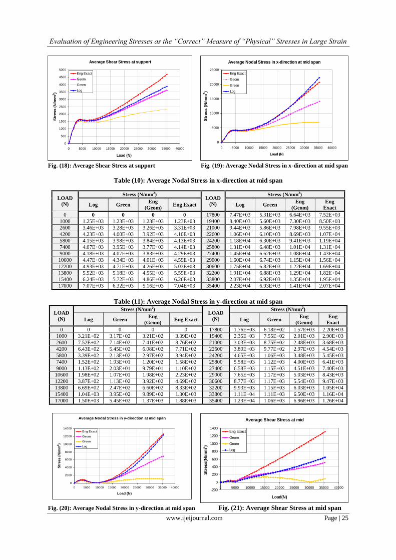
Tables (10), (11) and (12) show the values for average nodal stresses at mid-span. Very large loads

were applied in example resulting in large strains.

There is a marked difference between the Green and the other formulations’ values for the stresses at

the support for large load values. This is expected for cases of large strain. The Eng Exact values are the closest

to the Log (Cauchy) values for direct stresses. A similar trend is shown by the values of the stresses in the x-

direction at mid span with a maximum percentage difference between the Eng Exact and Log values of about

7% (around 69% for the Green and 37% for Eng). The stress at mid-span in the y-direction shows a similar

variation with the Eng Exact and Log values in close agreement and continuously increasing and the Green

values almost constant and close to zero. The maximum difference between the Eng Exact values and Eng

values is around 45%. This clearly shows the effect of assuming that the shear strain is small. The Eng Exact

shear stresses at mid-span values are large, compared to the other values, and are almost of a linear variation.

The Log and Eng shear values are in close agreement. This results from the assumption that the shear strain is

small in these formulations. The Green shear values at mid-span are very small compared to the values from the

other formulations and are of a non- uniform alternating nature. Thus, the Green strain formulation is not

suitable for evaluating the correct physical stresses. Also, the assumption that the shear strain is small limits the

use of the approximate Eng formulation for cases of small strain. Table (13) and Figure (22) show the maximum

principal stresses at mid-span for the Log and Eng Exact formulations. These are almost identical with a

maximum difference of about 6%. Hence, the stresses obtained using the Eng Exact formulation are considered

to be the correct measure of the physical stresses in large strain GNL.

Fig. (16): Average Nodal Stress in x-direction at support Fig. (17): Average Nodal Stress in y-direction at support

Average Nodal Stress in y-direction at support

0

500

1000

1500

2000

2500

3000

0 5000 10000 15000 20000 25000 30000 35000 40000

Load (N)

Str

es

s (

N/m

m2)

Eng Exact

Geom

Green

Log

L = 200 mm

y P

x D = 10 mm


0

1000

2000

3000

4000

5000

6000

7000

8000

9000

0 5000 10000 15000 20000 25000 30000 35000 40000

Load (N)

Str

ess (

N/m

m2)

Eng Exact

Geom

Green

Log



Fig. (18): Average Shear Stress at support Fig. (19): Average Nodal Stress in x-direction at mid span



LOAD

(N)

Stress (N/mm2) LOAD

(N)

Stress (N/mm2)

Log Green Eng

(Geom) Eng Exact Log Green

Eng

(Geom)

Eng

Exact

0 0 0 0 0 17800 1.76E+03 6.18E+02 1.57E+03 2.20E+03

1000 3.21E+02 3.17E+02 3.21E+02 3.39E+02 19400 2.35E+03 7.55E+02 2.01E+03 2.90E+03

2600 7.52E+02 7.14E+02 7.41E+02 8.76E+02 21000 3.03E+03 8.75E+02 2.48E+03 3.68E+03

4200 6.43E+02 5.45E+02 6.08E+02 7.71E+02 22600 3.80E+03 9.77E+02 2.97E+03 4.54E+03

5800 3.39E+02 2.13E+02 2.97E+02 3.94E+02 24200 4.65E+03 1.06E+03 3.48E+03 5.45E+03

7400 1.52E+02 1.93E+01 1.20E+02 1.58E+02 25800 5.58E+03 1.12E+03 4.00E+03 6.41E+03

9000 1.13E+02 2.03E+01 9.79E+01 1.10E+02 27400 6.58E+03 1.15E+03 4.51E+03 7.40E+03

10600 1.98E+02 1.07E+01 1.98E+02 2.23E+02 29000 7.65E+03 1.17E+03 5.03E+03 8.43E+03

12200 3.87E+02 1.13E+02 3.92E+02 4.69E+02 30600 8.77E+03 1.17E+03 5.54E+03 9.47E+03

13800 6.69E+02 2.47E+02 6.60E+02 8.33E+02 32200 9.93E+03 1.15E+03 6.03E+03 1.05E+04

15400 1.04E+03 3.95E+02 9.89E+02 1.30E+03 33800 1.11E+04 1.11E+03 6.50E+03 1.16E+04

17000 1.50E+03 5.45E+02 1.37E+03 1.88E+03 35400 1.23E+04 1.06E+03 6.96E+03 1.26E+04

Fig. (20): Average Nodal Stress in y-direction at mid span Fig. (21): Average Shear Stress at mid span


0

5000

10000

15000

20000

25000

0 5000 10000 15000 20000 25000 30000 35000 40000

Load (N)

Str

ess (

N/m

m2)

Eng Exact

Geom

Green

Log

Average Shear Stress at mid

-200

0

200

400

600

800

1000

1200

1400

0 5000 10000 15000 20000 25000 30000 35000 40000

Load(N)

Str

ess(N

/mm

2)

Eng Exact

Geom

Green

Log

LOAD

(N)

Stress (N/mm2) LOAD

(N)

Stress (N/mm2)

Log Green Eng


Eng

(Geom)

Eng

Exact

0 0 0 0 0 17800 7.47E+03 5.31E+03 6.64E+03 7.52E+03

1000 1.25E+03 1.23E+03 1.23E+03 1.23E+03 19400 8.40E+03 5.60E+03 7.30E+03 8.50E+03

2600 3.46E+03 3.28E+03 3.26E+03 3.31E+03 21000 9.44E+03 5.86E+03 7.98E+03 9.55E+03

4200 4.23E+03 4.00E+03 3.92E+03 4.10E+03 22600 1.06E+04 6.10E+03 8.69E+03 1.07E+04

5800 4.15E+03 3.98E+03 3.84E+03 4.13E+03 24200 1.18E+04 6.30E+03 9.41E+03 1.19E+04

7400 4.07E+03 3.95E+03 3.77E+03 4.14E+03 25800 1.31E+04 6.48E+03 1.01E+04 1.31E+04

9000 4.18E+03 4.07E+03 3.83E+03 4.29E+03 27400 1.45E+04 6.62E+03 1.08E+04 1.43E+04

10600 4.47E+03 4.34E+03 4.01E+03 4.59E+03 29000 1.60E+04 6.74E+03 1.15E+04 1.56E+04

12200 4.93E+03 4.71E+03 4.26E+03 5.03E+03 30600 1.75E+04 6.82E+03 1.22E+04 1.69E+04

13800 5.52E+03 5.18E+03 4.55E+03 5.59E+03 32200 1.91E+04 6.88E+03 1.29E+04 1.82E+04

15400 6.24E+03 5.72E+03 4.86E+03 6.26E+03 33800 2.07E+04 6.92E+03 1.35E+04 1.95E+04

17000 7.07E+03 6.32E+03 5.16E+03 7.04E+03 35400 2.23E+04 6.93E+03 1.41E+04 2.07E+04


0

500

1000

1500

2000

2500

3000

3500

4000

4500

5000

0 5000 10000 15000 20000 25000 30000 35000 40000

Load (N)

Str

ess (

N/m

m2)

Eng Exact

Geom

Green

Log


0

2000

4000

6000

8000

10000

12000

14000

0 5000 10000 15000 20000 25000 30000 35000 40000

Load (N)

Str

ess (

N/m

m2)

Eng Exact

Geom

Green

Log



Table (12): Average Shear Stress at mid span

LOAD

(N)

Stress (N/mm2) LOAD

(N)

Stress (N/mm2)

Log Green Eng


Eng

(Geom)

Eng

Exact

0 0 0 0 0 17800 2.42E+02 1.26E+02 2.45E+02 5.14E+02

1000 3.73E-01 1.12E+00 1.43E+00 1.87E+00 19400 2.70E+02 1.18E+02 2.63E+02 5.82E+02

2600 2.11E+01 1.31E+01 1.07E+01 3.90E+01 21000 3.01E+02 1.08E+02 2.82E+02 6.52E+02

4200 1.12E+01 2.21E+00 8.19E+00 2.74E+01 22600 3.33E+02 9.55E+01 3.01E+02 7.23E+02

5800 2.74E+01 4.11E+01 5.19E+01 3.50E+01 24200 3.66E+02 8.01E+01 3.21E+02 7.94E+02

7400 6.55E+01 7.47E+01 9.21E+01 1.03E+02 25800 4.02E+02 6.24E+01 3.42E+02 8.66E+02

9000 9.75E+01 9.85E+01 1.25E+02 1.66E+02 27400 4.38E+02 4.24E+01 3.63E+02 9.38E+02

10600 1.25E+02 1.14E+02 1.52E+02 2.27E+02 29000 4.76E+02 2.04E+01 3.87E+02 1.01E+03

12200 1.51E+02 1.24E+02 1.75E+02 2.88E+02 30600 5.16E+02 3.49E+00 4.12E+02 1.08E+03

13800 1.76E+02 1.29E+02 1.96E+02 3.50E+02 32200 5.57E+02 2.92E+01 4.40E+02 1.16E+03

15400 2.01E+02 1.31E+02 2.16E+02 4.14E+02 33800 5.99E+02 5.66E+01 4.70E+02 1.23E+03

17000 2.28E+02 1.28E+02 2.35E+02 4.80E+02 35400 6.43E+02 8.55E+01 5.02E+02 1.31E+03

Table (13) Maximum Principal Stress at Mid-span

LOAD

(N)

Stress (N/mm2)

LOAD

Stress (N/mm2)

LOAD

(N)

Stress (N/mm2)

Log Eng

Exact Log

Eng

Exact Log

Eng

Exact

0 0.0 0.0 12200 4935.0 5048.0 24200 11819.0 11996.0

1000 1250.0 1230.0 13800 5526.0 5616.0 25800 13121.0 13210.0

2600 3460.0 3311.0 15400 6248.0 6294.0 27400 14524.0 14425.0

4200 4230.0 4100.0 17000 7079.0 7084.0 29000 16027.0 15740.0

5800 4150.0 4130.0 18600 7931.0 8054.0 30600 17530.0 17054.0

7400 4071.0 4143.0 20200 8923.0 9076.0 32200 19134.0 18371.0

9000 4182.0 4297.0 21800 10015.0 10178.0 33800 20737.0 19687.0

10600 4474.0 4602.0 23400 11217.0 11390.0 35400 22341.0 20907.0

Fig. (22) Maximum Principal Stress at Mid-span

IV. CONCLUSIONS Based on the results of the numerical examples, it can be concluded that:

1. The Total Lagrangian solutions based on the Green strains and 2nd

Piola-Kirchhoff stresses while being not

suitable for evaluating the correct physical stresses are necessary for use as a base for the solutions based on

Engineering stresses.

2. The exact Engineering strain based formulation results in correct physical stresses, which are very close to

the true Cauchy stresses especially for small and moderately large strains. Bearing in mind the fact that the

elastic constants are evaluated using these stresses, these formulations must be used when stresses are

required in a Total Lagrangian analysis.

3. The formulation based on approximate Engineering strains give excellent results in structures wherein the

shear strains are small.

Max. Principal stress at mid-span

0

5000

10000

15000

20000

25000

0 5000 10000 15000 20000 25000 30000 35000 40000

Load (N)

Str

ess (

N/m

m2)

Log

Eng Exact



4. The use of Logarithmic strains is necessary when the exact true stresses are required. The results from the

Log formulation presented here can be further enhanced by removing the restriction of small shear strains.

5. The formulation based on the exact Engineering strains can be easily extended to three-dimensional

analysis.

REFRENCES [1] Yang, Y. B. and Kuo, S. R., Theory and Analysis of Nonlinear Framed Structures, Prentice Hall, Simon & Schuster (Asia), 1998,

Singapore.

[2] Crisfield, M. A., Non-linear Finite Element Analysis of Solids and Structures, Volume 1, John Wiley & Sons Ltd., August 1997,

Chichester, England. [3] Zienkiewicz O. C. and Taylor, R. L., The Finite Element Method for Solids and Structural Mechanics, 6th edition , Butterworth

Heinemann 2005, Elsevier.

[4] Mohamed, A. E., A Small Strain Large Rotation Theory and Finite Element Formulation of Thin Curved Beams, Ph.D. Thesis, 1983, The City University, London.

[5] Belytschko, T., Finite Elements for Nonlinear Continua & Structures, North-Westren University, 1998, Evanston.

[6] Marinkovic`, D., Koppe, H. and Gabbert, U., Degenerated shell element for geometrically nonlinear analysis of thin-walled piezoelectric active structures, Smart Mater. Struct. 17, 2008, 015030 (10pp), IOP Publications, G.B.

[7] Wood, R. D. and Zienkiewicz, O. C., Geometrically Nonlinear Finite Element Analysis of Beams, Frames, Arches and Axisymmetric

Shells, Computers & Structures, 1977, Vol.7, pp 725-735, PergamonPress, G.B. [8] Surana, K. S. and Sorem, R. M., Geometrically Nonlinear Formulation for Three Dimensional Curved Beam Elements with Large

Rotations, Int. J. Num. Meth. Engng., 1989, Vol.28, 43-73.

[9] Djermane, M., Chelghoum, A. ,Amieur, B. and Labbaci, B., Linear and Nonlinear Thin Shell Analysis using a Mixed Finite with Drilling Degrees of Freedom, Int. J. Applied Engng. Research, 2006, Vol. 1 No. (2) pp 217-236.

[10] Bonet, J. and Wood, R.D., Nonlinear Continuum Mechanics for Finite Element Analysis, CambridgeUniversity Press, 1997, Cambridge, U.K.

[11] Mohamed, A. E. and Adam, F. M., Large Deformation Finite Element Analysis of Shell Structures, Journal of Science &

Technology, June 2003, Vol.4-No. 2, 47-58, SUST, Khartoum, Sudan. [12] Adam, F. M. and Elzubair, A., Large Deformation Finite Element Analysis of Shells, Degenerated Eight Nodes Shell Element, LAP

LAMBERT Academic Publishing, 2012, Germany.

[13] Akasha Hilal, N. M., Development of Geometrically Nonlinear Finite Element Program using Plane Stress/Strain Elements based on Engineering and True Stress Measures, Ph. D. Thesis, SUST, October 2009, Khartoum, Sudan.

[14] Akasha, N. M. and Mohamed, A. E., Geometrically Nonlinear Analysis using Plane Stress/Strain Elements based on Alternative

Strain Measures”, Journal of Science & Technology; Engng. Comp. Sciences, June 2012, Vol. 13- No. 1- 1-12, SUST, Khartoum, Sudan.

[15] Akasha, N. M. and Mohamed, A. E., Evaluation of Engineering Stress for Geometrically Nonlinear Plane Stress/Strain Problems,

JASER, June 2012, Vol. 2, No. 2, , 115-125, Design for Scientific Renaissance. [16] Greco, M. and Ferreira, I. P., Logarithmic strain measure applied to the nonlinear formulation for space truss analysis, Finite

Elements in Analysis and Design, 2009, 45, 632-639.

[17] Akasha, N. M. and Mohamed, A. E., Evaluation of True Stress for Geometrically Nonlinear Plane Stress/Strain Problems, JASER, March 2012, Vol.2, No.1, 68-79, Design for Scientific Renaissance.

evaluation of engineering stresses as the “correct” measure of “physical” stresses in large...

Technology

exact engineering stresses

civil engineering

mentioned stresses

exact engineering strains

exact engineering geometric

nonlinear problems

true cauchy stresses

lagrangian formulations