Steady Couette flows of elastoviscoplastic fluids arenon-unique

I. Cheddadi1, P. Saramito2, and F. Graner3,4

1INRIA Paris - Rocquencourt, BANG team, Domaine de Voluceau,Rocquencourt, B.P. 105, 78153 Le Chesnay, France

ibrahim.cheddadi@inria.fr

2Laboratoire Jean Kuntzmann, UMR 5524 Univ. J. Fourier - Grenoble Iand CNRS, BP 53, F-38041 Grenoble cedex, France

3BDD, Institut Curie, CNRS UMR 3215 and INSERM U 934, 26 rued’Ulm, F-75248 Paris cedex 05, France

4Matiere et Systemes Complexes (MSC), UMR 7057 CNRS & UniversiteParis Diderot, 10 rue Alice Domon et Leonie Duquet, 75205 Paris Cedex 13,

France

Abstract

The Herschel-Bulkley rheological fluid model includes terms representing viscosityand plasticity. In this classical model, below the yield stress the material is strictlyrigid. Complementing this model by including elastic behaviour below the yield stressleads to a description of an elastoviscoplastic (EVP) material such as an emulsionor a liquid foam. We include this modification in a completely tensorial descriptionof cylindrical Couette shear flows. Both the EVP model parameters, at the scaleof a representative volume element, and the predictions (velocity, strain and stressfields) can be readily compared with experiments. We perform a detailed study of theeffect of the main parameters, especially the yield strain. We discuss the role of thecurvature of the cylindrical Couette geometry in the appearance of localisation; wedetermine the value of the localisation length and provide an approximate analyticalexpression. We then show that, in this tensorial EVP model of cylindrical Couetteshear flow, the normal stress difference strongly influences the velocity profiles, whichcan be smooth or non-smooth according to the initial conditions on the stress. Thisfeature could explain several open questions regarding experimental measurements on

1

eθ

er

y

x

(a) (b)

r0

re

V

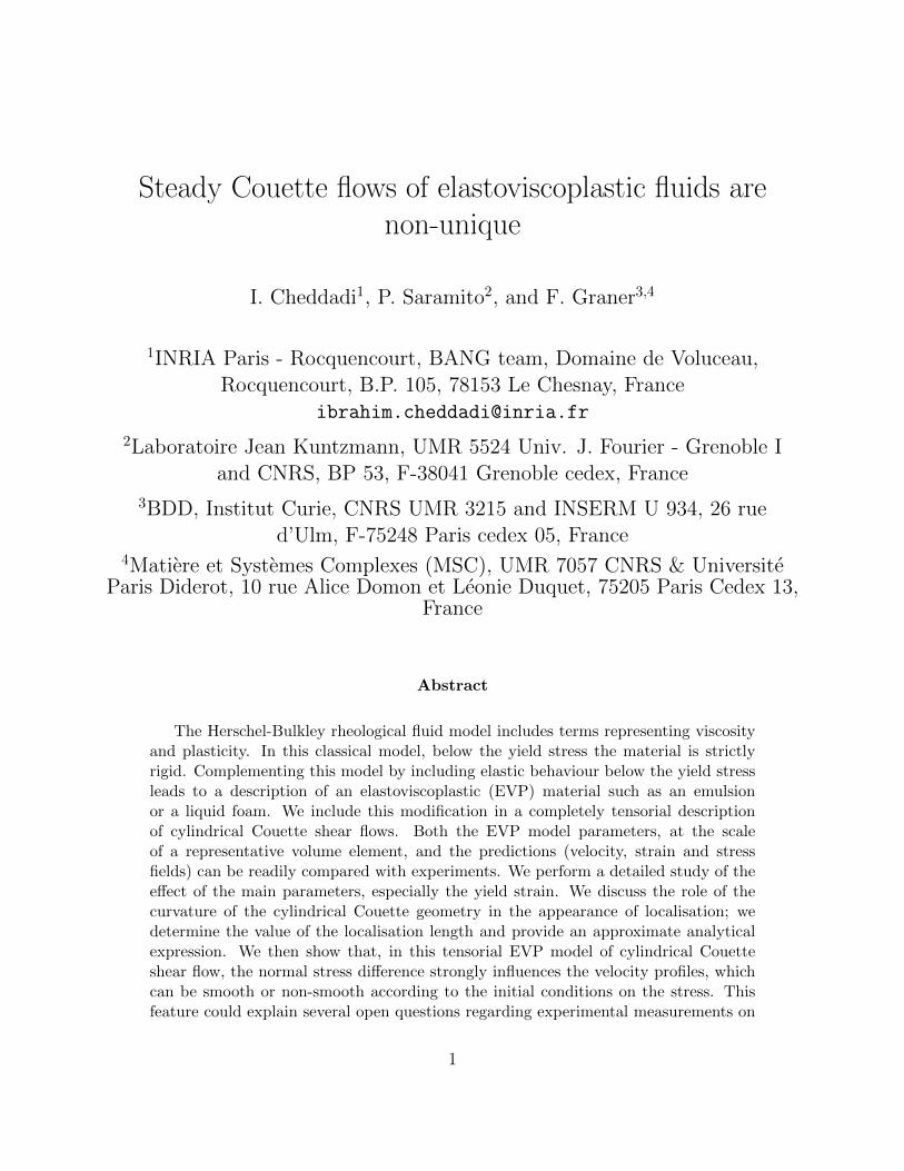
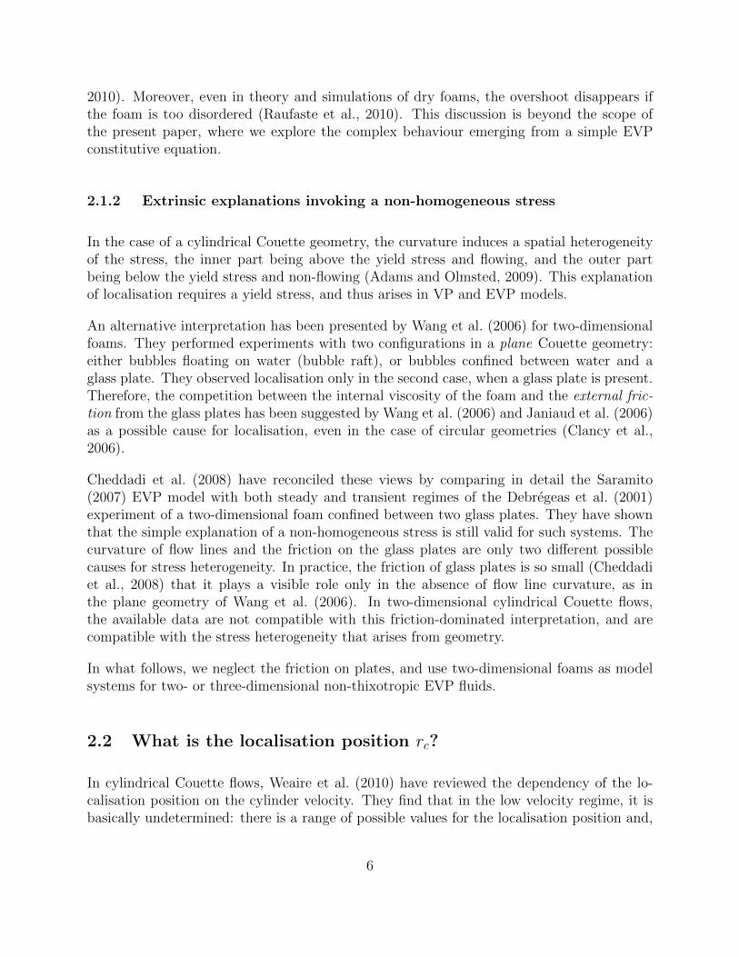
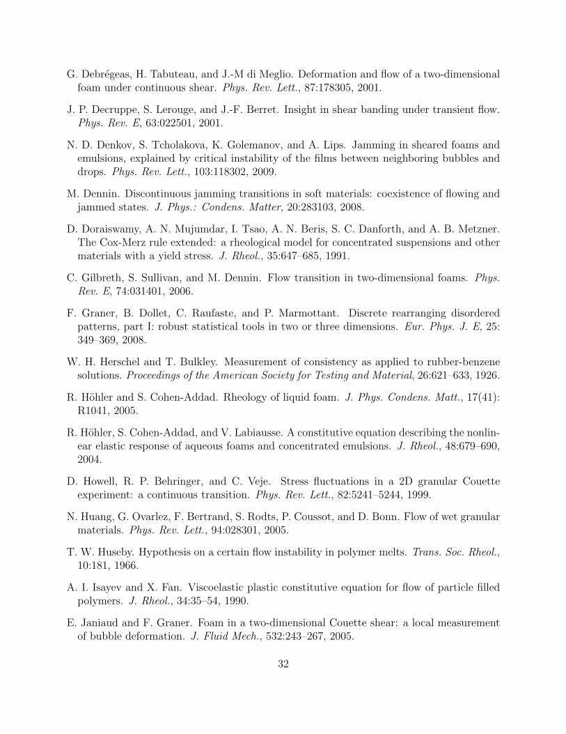
Figure 1: Experimental set-up for a two-dimensional circular shear flow of a foam confinedbetween two horizontal plates. (a) definition of the geometric and kinematic parameters ;(b) picture of the confined two-dimensional liquid foam (from Debregeas et al. (2001)): theinternal radius is r0 = 71 mm.

Couette flows for various EVP materials such as emulsions or liquid foams, includingthe non-reproducibility that has been reported in flows of foams. We then discussthe suitability of Couette flows as a way to measure rheological properties of EVPmaterials.

Keywords: elastoviscoplastic / viscoelastoplastic fluids ; non-Newtonian fluids ; Couetteexperiment ; liquid foam ; suspensions ; mathematical modelling.

1 Introduction

Localisation is a phenomenon often observed in two- or three-dimensional shear flows ofcomplex materials: Coussot et al. (2002) observed it for emulsions, Salmon et al. (2003a)for colloids, and Howell et al. (1999); Mueth et al. (2000); Losert et al. (2000); Huang et al.(2005) for wet granular materials. It consists of a coexistence between a region localisednear a moving boundary, where the material flows like a liquid, and another region wherethe material behaves like a solid.

Since the pioneering experiment of Debregeas et al. (2001) (Fig. 1), liquid foams (gas bubblesdispersed within a continuous liquid phase, as explained by Weaire and Hutzler (1999) andCantat et al. (2010)) have been widely used for experimental, theoretical and numericalstudies of localisation (for reviews see e.g. Hohler and Cohen-Addad (2005); Schall and van

2

Hecke (2010); Barry et al. (2011)). Their discrete units, the gas bubbles, are easy to observe(especially in two dimensions) and to manipulate. Moreover, they display simultaneouselastic, viscous, plastic behaviours (referred to as elastoviscoplastic, or EVP), thus coveringa wide range of behaviours observed in many complex materials.

The aim of this paper is to show that including tensorial elasticity in the classical viscoplasticHerschel-Bulkley (VP) model leads to many improvements in the understanding of Couetteflows of non-thixotropic EVP fluids such as emulsions, liquid foams, or carbopol gel. Thesematerials exhibit normal stresses that arise from the local anisotropy (hence the necessityof a tensorial description) of the elasticity related to their micro-structure. Localisationcan appear if the material yields, that is, if the material is plastic; in the regions belowthe yield strain, the normal stresses can remain finite even in a steady-state flow. If, inaddition, viscous dissipation occurs during plastic events, elasticity is coupled to viscosity inthe flowing region, so that the normal stresses are coupled to the velocity gradient, even inthe Couette geometry.

Cheddadi et al. (2008, 2009, 2011a) have previously explored this approach with the Saramito(2007) model (Bingham-like plastic dissipation), for cylindrical Couette flows of liquid foamsand other EVP flows around an obstacle; they have successfully explained the observationsof normal stresses components measured by Janiaud and Graner (2005) in the experimentaldata of Debregeas et al. (2001).

In the present work, the theoretical predictions of the Saramito (2009) model are comparedwith experimental measurements, including shear and normal stresses when available. Thismodel is an extension of the Saramito (2007) model, that includes a Herschel-Bulkley-likeplastic dissipation.

We study the influence of the dimensionless rheological parameters, including the yield strainand the cylindrical Couette geometry curvature (introduced in section 3). For simplicity, wefocus here on the low velocity regime corresponding to most published foam Couette flowexperiments; we postpone, for future work, analysis of both the quasistatic regime whereviscosity plays no visible role, studied in simulations (Wyn et al., 2008; Raufaste et al., 2010),and the high velocity regime where viscous and friction effects are dominant (see e.g. Katgertet al. (2008, 2009, 2010)). The inclusion of elasticity and of tensorial description are twoessential features of the present modelling, leading to three predictions not captured by scalarand/or VP models. First, we show that normal stresses that depend on the preparation ofthe material (Labiausse et al., 2007) can persist as residues even in steady flow. Second,we predict that velocity flow profiles are either smooth or non-smooth depending on themeasured value of the stress tensor. Third, as a consequence of these two results, two- andthree-dimensional cylindrical Couette flows of EVP materials are non-unique, even in steadystate. To summarise, the effect we describe in this paper is not specific to a given materialmicrostructure, but is more generally a consequence of the material’s visco-elasto-plasticityand of the specifically tensorial nature of the Couette flow.

3

The outline of the paper is as follows. Section 2 reviews and discusses the main open ques-tions found in the literature, which we address here. Section 3 discusses some constitutiveequations for EVP materials, in particular the EVP model of Saramito (2009). Section 4presents the solutions of this model and some of the main features which are absent fromVP models: the effect of initial conditions, memory effects, non-uniqueness, and non-smoothsolutions; we also explain how such EVP model can be compared to actual experimentaldata. Section 5 examines how variations of the EVP model parameters affect these flowfeatures, and provides an approximate analytical expression for the localisation length (eq.15). Section 6 discusses the consequences of our results. Section 7 summarises our findings.

2 Open questions

During the last ten years there has been extensive debate on the Couette flow of variouscomplex fluids, raising some theoretical questions (see eg. Schall and van Hecke (2010)):

• What is the physical origin of localisation?

• Where does the material localise?

• Why do some experiments report smooth profiles at the localisation position and someothers experiments report non-smooth ones?

Before we examine the status of these questions, we first need to clarify the vocabulary andhypotheses used in the literature:

• We assume here that the materials of interest can be described using continuum me-chanics: this implies that there is a representative volume element (RVE). The RVEshould be smaller than the scale of the global flow, but large enough so that one candefine: (i) variables such as stresses, strains, velocity gradient; and (ii) parameters,such as elastic modulus, yield strain and viscosity. Note that in an EVP materialstress, strain and deformation rate are variables which can be independently defined,and measured in situ if the material can be imaged in full details (Graner et al., 2008).

• Since the phrase “shear banding” (Vermant, 2001) is used to describe different things,we prefer not to use it. We instead use “smooth” (resp: “non-smooth”) to indicatethat the velocity gradient is continuous (resp: discontinuous).

• The word “localisation” is a historical term used consistently to mean “coexistence ofrigid and flowing regions”. We thus use it here.

4

• In cylindrical Couette flows the localisation radius, denoted as rc, admits several pos-sible definitions (see Gilbreth et al. (2006) or section 7.3 of Weaire et al. (2010)). Here,we choose to define rc as the position separating the flowing region from the rigid one,or equivalently as the limiting value of the radius at which the deformation rate is zero.

• There are at least two different ways, one in mathematics and one in rheology, usedto define the norm of a tensor, and thus the von Mises criterion regarding the yieldstrain and stress: we choose the mathematical one, presented below (see eq. (4) anddiscussion thereafter).

2.1 What is the physical origin of the localisation?

There are several explanations for the origin of the localisation; many of them are reviewedand discussed by Schall and van Hecke (2010).

Coussot et al. (2002) used MRI methods to measure the local velocity in three-dimensionalcylindrical Couette flows of other EVP materials such as carbopol gel, and more generallyyield stress fluids such as bentonite suspensions and cement paste. Despite the apparentsimplicity of shear flows, a common description of these experiments is still lacking (seeOvarlez et al. (2009) for a review): on the one hand, thixotropic materials exhibit an intrinsiccritical shear rate, i.e. these materials cannot flow homogeneously at a shear rate smaller thana critical value, which is characteristic of the material; on the other hand, non-thixotropicmaterials may or may not exhibit a critical shear rate (that does not seem to be intrinsic tothe material), as discussed below in section 2.3. We focus here on non-thixotropic materialsand try to explain this peculiar behaviour.

2.1.1 Intrinsic explanations invoking a non-monotonic constitutive equation

In complex materials which display a shear-induced structural transition, a possible source oflocalisation is the coexistence of two different shear rates at the same stress, that is, the shearstress versus shear rate curve is multi-valued (Huseby, 1966; Berret et al., 1994; Porte et al.,1997; Decruppe et al., 2001; Benito et al., 2010). In fact, foam experiments (Khan et al.,1988) and simulations (Kabla et al., 2007; Okuzono and Kawasaki, 1995; Raufaste et al.,2010) suggest that in the quasi-static regime the shear stress versus shear strain curve passesthrough an overshoot before reaching a plateau, thus being multi-valued (Clancy et al., 2006;Weaire et al., 2009, 2010).

This explanation is probably not generally applicable to foams in Couette experiments: foamsusually contain at least a few percent liquid, so that their yield strain is lower than for ideallydry foams (Marmottant et al., 2008) and the overshoot becomes undectable (Raufaste et al.,

5

2010). Moreover, even in theory and simulations of dry foams, the overshoot disappears ifthe foam is too disordered (Raufaste et al., 2010). This discussion is beyond the scope ofthe present paper, where we explore the complex behaviour emerging from a simple EVPconstitutive equation.

2.1.2 Extrinsic explanations invoking a non-homogeneous stress

In the case of a cylindrical Couette geometry, the curvature induces a spatial heterogeneityof the stress, the inner part being above the yield stress and flowing, and the outer partbeing below the yield stress and non-flowing (Adams and Olmsted, 2009). This explanationof localisation requires a yield stress, and thus arises in VP and EVP models.

An alternative interpretation has been presented by Wang et al. (2006) for two-dimensionalfoams. They performed experiments with two configurations in a plane Couette geometry:either bubbles floating on water (bubble raft), or bubbles confined between water and aglass plate. They observed localisation only in the second case, when a glass plate is present.Therefore, the competition between the internal viscosity of the foam and the external fric-tion from the glass plates has been suggested by Wang et al. (2006) and Janiaud et al. (2006)as a possible cause for localisation, even in the case of circular geometries (Clancy et al.,2006).

Cheddadi et al. (2008) have reconciled these views by comparing in detail the Saramito(2007) EVP model with both steady and transient regimes of the Debregeas et al. (2001)experiment of a two-dimensional foam confined between two glass plates. They have shownthat the simple explanation of a non-homogeneous stress is still valid for such systems. Thecurvature of flow lines and the friction on the glass plates are only two different possiblecauses for stress heterogeneity. In practice, the friction of glass plates is so small (Cheddadiet al., 2008) that it plays a visible role only in the absence of flow line curvature, as inthe plane geometry of Wang et al. (2006). In two-dimensional cylindrical Couette flows,the available data are not compatible with this friction-dominated interpretation, and arecompatible with the stress heterogeneity that arises from geometry.

In what follows, we neglect the friction on plates, and use two-dimensional foams as modelsystems for two- or three-dimensional non-thixotropic EVP fluids.

2.2 What is the localisation position rc?

In cylindrical Couette flows, Weaire et al. (2010) have reviewed the dependency of the lo-calisation position on the cylinder velocity. They find that in the low velocity regime, it isbasically undetermined: there is a range of possible values for the localisation position and,

6

moreover, the size of this range diverges when the velocity decreases. There are two ques-tions: is there a hidden variable which fixes the localisation position? for a given experiment,is the position predictable?

To answer these questions, in section 5 we explicitly determine the localisation position, andstudy its dependence on model parameters and initial conditions.

2.3 Why smooth and/or non-smooth profiles?

0

0.5

1

0 0.1 0.2 0.3 0.4 0.5r−r0∆r

vθ(r)

V

(a)

liquid foam, exp.present computation

0

0.5

1

0 0.25 0.5 0.75 1r−r0∆r

vθ(r)

V(b)

0

0.05

0.1

0.15

0.2 0.3

suspension 4.6%, exp.present computation

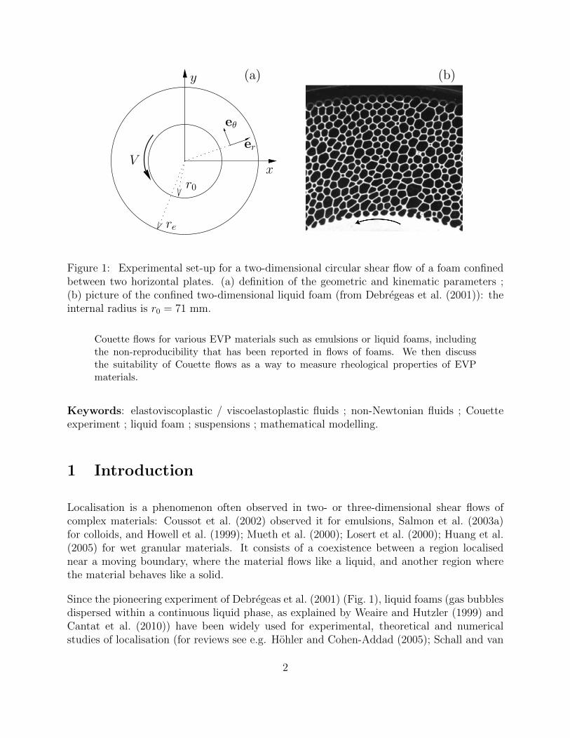
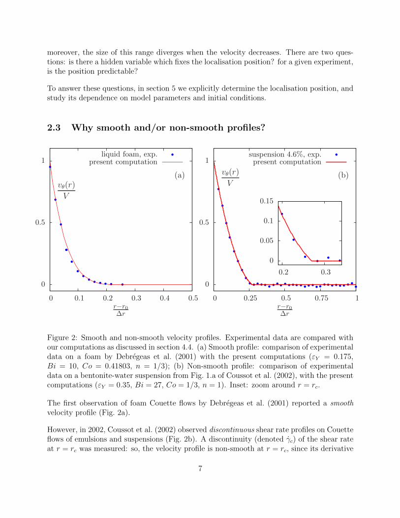
Figure 2: Smooth and non-smooth velocity profiles. Experimental data are compared withour computations as discussed in section 4.4. (a) Smooth profile: comparison of experimentaldata on a foam by Debregeas et al. (2001) with the present computations (εY = 0.175,Bi = 10, Co = 0.41803, n = 1/3); (b) Non-smooth profile: comparison of experimentaldata on a bentonite-water suspension from Fig. 1.a of Coussot et al. (2002), with the presentcomputations (εY = 0.35, Bi = 27, Co = 1/3, n = 1). Inset: zoom around r = rc.

The first observation of foam Couette flows by Debregeas et al. (2001) reported a smoothvelocity profile (Fig. 2a).

However, in 2002, Coussot et al. (2002) observed discontinuous shear rate profiles on Couetteflows of emulsions and suspensions (Fig. 2b). A discontinuity (denoted γc) of the shear rateat r = rc was measured: so, the velocity profile is non-smooth at r = rc, since its derivative

7

is related to the shear rate. Such non-smooth profiles were found by others between 2003and 2008: for worm-like micelles by Salmon et al. (2003a), for lyotropic lamellar systemsby Salmon et al. (2003b), for Couette foam flows by Lauridsen et al. (2004); Gilbreth et al.(2006); Dennin (2008); Krishan and Dennin (2008), and interpreted theoretically by Denkovet al. (2009); Clancy et al. (2006); Weaire et al. (2010).

Surprisingly, in 2008-2010, experiments published by Katgert et al. (2008, 2009, 2010), Cous-sot and Ovarlez (2010), and Ovarlez et al. (2010) showed smooth velocity profiles and contin-uous shear rates at r = rc: γc equals zero. Note that some papers with contradictory resultsshared either an author (Coussot et al., 2002; da Cruz et al., 2002; Huang et al., 2005; Cous-sot and Ovarlez, 2010) or a set-up, the bubble raft (Lauridsen et al., 2004; Gilbreth et al.,2006; Dennin, 2008; Krishan and Dennin, 2008; Katgert et al., 2008, 2009, 2010).

Coussot and Ovarlez (2010) explained this discrepancy by questioning the quality of theexperiments: “previous data on a specific foam (Rodts et al., 2005) were probably affectedby experimental artefacts”. Similarly, Ovarlez et al. (2010) explain that “Our measurementsdemonstrate that three-dimensional foams do not exhibit observable signatures of [discontin-uous] shear banding. This contrasts with the results of Rodts et al. (2005) and da Cruz et al.(2002) which we have shown to pose several experimental problems” and mention that “thecase of bubble rafts is still unclear”.

Our results emphasise the intrinsic sensitivity of the equations to the sample history (Benitoet al., 2010); this could explain why experimental artifacts such as impurities (Rodts et al.,2005) or bubble rupture (da Cruz et al., 2002) could yield drastic changes in observations.Even when experimental artifacts are eliminated, our results regarding the effect of trappedstresses due to initial conditions provide a deep reason to explain why, according to theset-up or foam preparation, either a smooth or a non-smooth profile could appear.

3 Constitutive equation

3.1 Brief review of EVP models

A number of closely related models have appeared in the literature (see Saramito (2007)for a review). Table 1 distinguishes models with respect to their behaviour before and afteryielding, their applicability to three-dimensional general flows, and to the existence of a proofthat the dissipation is positive.

We now discuss the mathematical formulation and properties of some of these models. Theequations are written in two dimensions with polar coordinates to fit with the cylindricalCouette geometry. Table 2 lists the corresponding dimensionless parameters. In each model

8

contribution before yielding after yielding 3D TH

Schwedoff (1900) rigid solid VE fluidBingham (1922) rigid solid Newtonian fluid X XHerschel and Bulkley (1926) rigid solid power-law fluid X XOldroyd (1947) elastic solid Newtonian fluid X XIsayev and Fan (1990) elastic solid VE fluid X XDoraiswamy et al. (1991) elastic solid power-law fluid XPuzrin et al. (2003) elastic solid VE solid X XSaramito (2007) VE solid VE fluid X XBenito et al. (2008) VE solid VE fluid X XSaramito (2009) VE solid power-law VE fluid X X

Table 1: Summary of the referenced EVP models. The 3D column is marked when the modelhas been written in a general tensorial sense, e.g. with objective derivatives. The TH columnis also marked when the model has a positive dissipation according to the second law ofthermodynamics. The italic mark X in the 3D or the TH columns means that the corre-sponding property was derived after publication of this model. For instance, the Binghamand the Herschel-Bulkley models were first proposed in a one-dimensional simple shear flowcontext, then extended to three dimensions, and finally found to satisfy the second law ofthermodynamics.

the constitutive equation is closed with equations for momentum and mass balance, andappropriate Couette flow boundary and initial conditions. Since external forces and inertiaare negligible here (see section 2.1 and Cheddadi et al. (2008)), the momentum balancereduces to

∇ · τ = 0, (1)

where τ is the stress tensor. The material is assumed to be incompressible, so the massbalance is

∇ · v = 0, (2)

where v is the velocity.

3.2 VP model: Herschel-Bulkley

Herschel and Bulkley (1926) proposed a power-law variant of the viscoplastic Bingham (1922)

9

symbol name definition physical meaning typical range

εY yield strainτY2G

(eq. 11) elastoplasticity [0, 0.5]

Bi BinghamτY ∆r

ηV(eq. 5) viscoplasticity [0, 100]

Co curvaturere − r0

re(eq. 6) curvature ]0, 1[

n power-law index (eq. 3) shear thinning [0.3, 1]

We WeissenbergηV

G∆r=

2εYBi

(eq. 9) viscoelasticity [0, 0.04]

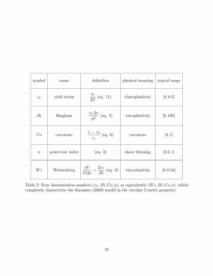
Table 2: Four dimensionless numbers (εY , Bi, Co, n), or equivalently (We,Bi, Co, n), whichcompletely characterise the Saramito (2009) model in the circular Couette geometry.

10

model (see also Oldroyd (1947)): τ = 2K|D|n−1D + τYD

|D| when |D| 6= 0,

|τd| ≤ τY otherwise,

or equivalently: max

(0,|τd| − τY2K|τd|n

) 1n

τ = D, (3)

where D = (∇v + ∇vT )/2 is the deformation rate tensor, |D| =√DijDij its Euclidian

norm, and (∇v)ij = (∂jvi) is the velocity gradient tensor. The so-called deviatoric stress τdis defined according to the spatial dimension in which the flow is investigated: τd = τ − 1

NI,

where I is the identity matrix, and N = 1, 2 or 3. We focus here on two-dimensional flowsand take N = 2. Here, τY > 0 is the yield stress, K > 0 is the consistency parameter, andn > 0 is the power-law index.

The von Mises criterion, |τd| ≤ τY , involves the Euclidian norm of the deviatoric part of thestress. In cylindrical coordinates it is written:

|τd| =(

2τ 2rθ +

(τrr − τθθ)2

2

) 12

. (4)

Note that, favouring the shear stress, some authors use a slightly different definition of

the deviatoric stress norm (Raufaste et al., 2010): (τ 2rθ + (τrr − τθθ)2/4)

12 . This rheological

definition would lead to an alternative, equivalent model: keeping the same equation(3), itwould only multiply the deviatoric stress norm |τd| by 2−1/2, the yield stress τY by 2−1/2,and the consistency K by 2(n−1)/2.

In the circular Couette geometry, V denotes the velocity of the inner cylinder and ∆r = re−r0

the width of the gap. Note that η = K(V/∆r)n−1 has the dimension of a viscosity and thatη = K when n = 1. The dimensionless Bingham number is

Bi =τY ∆r

ηV. (5)

It compares the yield stress τY with a characteristic viscous stress ηV/∆r. Let us alsointroduce the dimensionless number Co:

Co = 1− r0

re, (6)

that quantifies the curvature of the circular Couette geometry. When the two radii are close,this number is close to zero. Conversely, when the curvature is extreme, e.g. r0 becomessmall, this number tends to one.

The Herschel-Bulkley model predicts localisation in the circular Couette geometry, as a resultof the stress heterogeneity. Its position rc can be numerically computed (see appendix A,equation (16)).

11

The Herschel-Bulkley model reduces to the Bingham one when n = 1, to a power-law fluidwhen τY = 0, and to a Newtonian fluid when n = 1 and τY = 0. The shear thinningbehaviour is associated with 0 < n < 1 and the (less usual) shear thickening behaviour withn > 1.

3.3 VE model: Oldroyd

Oldroyd (1950) proposed the following viscoelastic model:

η

G

∇τ +τ = 2ηD, (7)

where G > 0 is the elastic modulus and η/G is a relaxation time. The total stress isσ = 2η2D+ τ where η2 is a second viscosity, often called the solvent viscosity in the contextof polymer solutions. When η2 = 0, the Oldroyd model reduces to the so-called Maxwell

model. The upper-convected tensorial derivative∇τ is defined by

∇τ=

∂τ

∂t+ v.∇τ − τ.∇vT −∇v.τ. (8)

The dimensionless Weissenberg number is

We =ηV

G∆r. (9)

It compares the characteristic viscous stress ηV/∆r with the elastic modulus G. When1/G = 0, the Oldroyd model reduces to a Newtonian one.

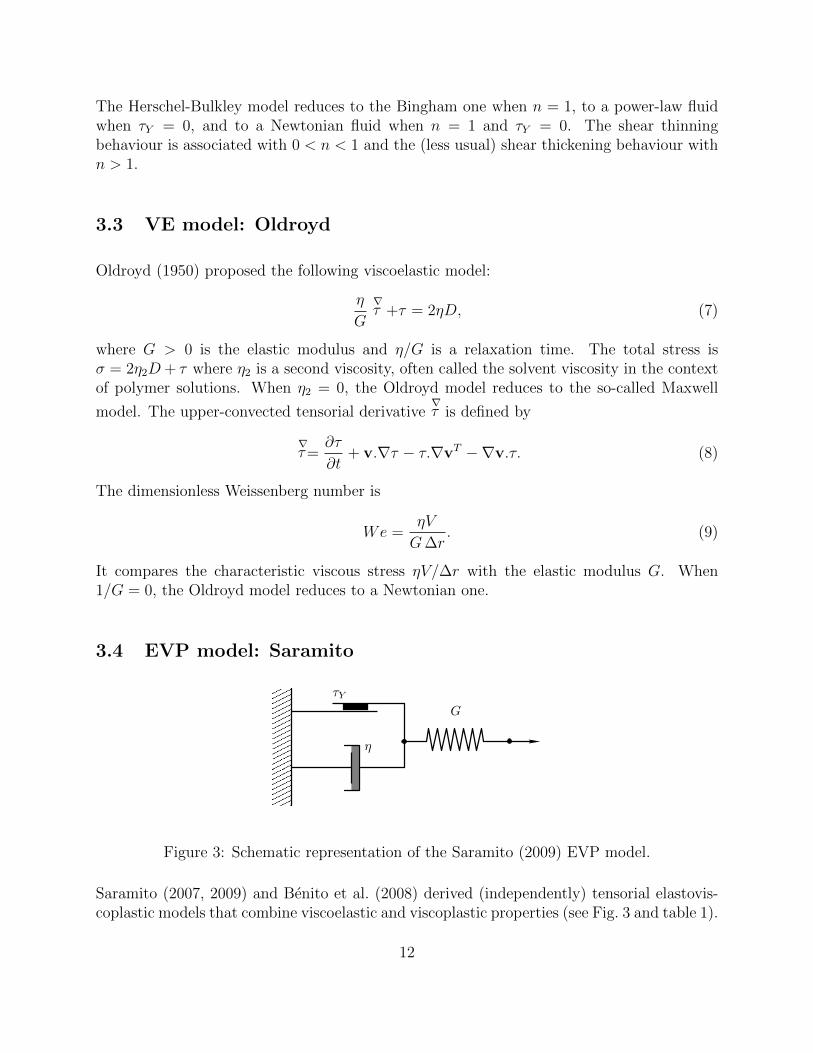
3.4 EVP model: Saramito

τY

η

G

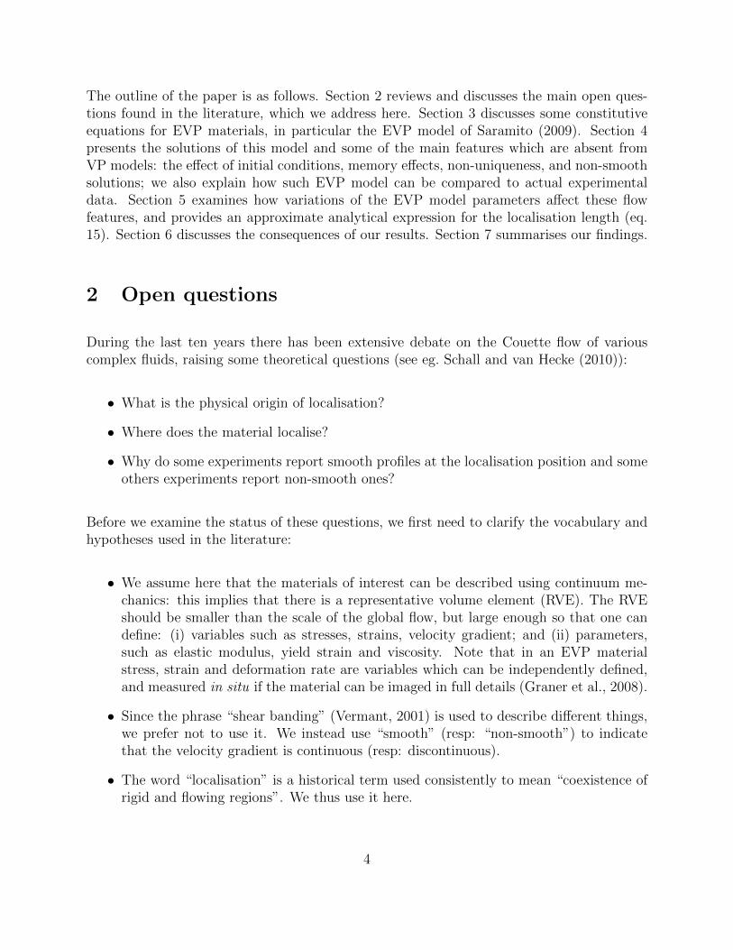
Figure 3: Schematic representation of the Saramito (2009) EVP model.

Saramito (2007, 2009) and Benito et al. (2008) derived (independently) tensorial elastovis-coplastic models that combine viscoelastic and viscoplastic properties (see Fig. 3 and table 1).

12

They satisfy the second law of thermodynamics and match the behaviour of non-thixotropicEVP materials like foams and emulsions: elastic solid before yielding and viscoelastic flowafter yielding.

The EVP model presented by Saramito (2009) is simple enough to allow for the numericalresolution (with good convergence, see appendix B) of the associated partial differentialequations even in intricate two- (Cheddadi et al., 2011a) and three-dimensional geometries,and is thus suitable for practical and industrial purposes. It is written:

1

2G

∇τ + max

(0,|τd| − τY2K|τd|n

) 1n

τ = D. (10)

When 1/G = 0 we obtain the Herschel-Bulkley model, eq. (3). Conversely, when n = 1 andτY = 0 we obtain the Oldroyd model, eq. (7). Finally, when both 1/G = 0, τY = 0 andn = 1, the model is Newtonian.

In addition to the independent dimensionless numbers (We,Bi, Co, n) already introducedfor the Herschel-Bulkley and Oldroyd models, we define the elastic yield strain εY as

εY =τY2G

=BiWe

2. (11)

This dimensionless parameter is a measure of the softness and deformability of the material.It has been shown to be the main parameter for the characterisation of EVP materials (Ched-dadi et al., 2011a) and is often easier to measure from experiments than the yield stress (Mar-mottant et al., 2008). The four independent dimensionless numbers (εY , Bi, Co, n) com-pletely characterise the problem (table 2), like (We,Bi, Co, n).

From now on, the Saramito (2009) model will be refered to as “the EVP model”, while theHerschel-Bulkley model will be refered to as “the VP model”.

4 Overview of the solutions of the EVP model

4.1 Homogeneous flows: transient response to a simple shear

Saramito (2007, 2009) studied simple flows in a geometry without stress heterogeneity, suchas uniaxial extensional flow, oscillating shear flow or simple shear flow. To enable comparisonwith the circular Couette geometry (section 4.2), we first study the prediction of the EVPmodel in simple shear flow. The fluid is initially at rest: at t = 0, τ = 0. Then for t > 0, aconstant shear rate γ is applied.

The solution τ(t) is then computed from eq. (10). As long as there is no stress heterogeneity,the EVP model does not predict any localisation. Figs. 4a,b plot the normalised shear

13

0

1

2

3

0 2 4 6 8

tγ

(a)η+S (t, γ)

Kγn−1

n = 1

n = 0.5n = 0.2

0

1

2

3

4

0 2 4 6 8

tγ

(b)N+1 (t, γ)

2Kγnn = 1

n = 0.5

n = 0.2

100

101

10−2 10−1 100 101 102

We = Kγn−1/G

n = 1 (c)ηS(γ)

Kγn−1

Bi = 4

Bi = 2Bi = 1

Bi = 0100

101

10−2 10−1 100 101 102

We

n = 0.5 (d)ηS(γ)

Kγn−1

Bi = 4

Bi = 2Bi = 1

Bi = 0

Figure 4: Start-up shear flow for We = ηγ/G = Kγn−1/G = 1 and Bi = τY /(Kγn) = 1:

(a) normalised shear stress growth coefficient η+S (t, γ) vs normalised time; (b) normalised

first normal stress difference N+1 (t, γ) vs normalised time. Steady shear flow: shear stress

coefficient ηS(γ) vs We for various values of Bi: (c) n = 1; (d) n = 0.5.

14

stress growth coefficient η+S = τ/γ and the first normal stress difference N1 = τ11 − τ22 with

respect to the applied shear γt. At first, when the stress in the material is still below theyield stress τY , the shear stress increases linearly with time while the first normal differenceincreases quadratically : the material behaves as an elastic solid obeying the Poynting law(Hohler et al., 2004). Such a non linear phenomenon has been seen experimentally in foams(Labiausse et al., 2007). After this initial elastic transient, saturation occurs at large appliedshear: the stress components tend to a constant value as the applied shear tends to infinity.At the transition to the steady state, one can observe an overshoot of the shear stress thatis more pronounced for small values of n.

Fig. 4c,d plot the steady shear viscosity ηS = limt→∞ η+S versus We. For 0 < n < 1, the

shear viscosity decreases monotonically while it tends to a plateau when n = 1. Thus, whenn < 1, the material is shear thinning. Observe that the value of Bi controls the viscosityplateau at small values of We while it has less influence on the viscosity for large values ofWe.

In summary, before yielding, the material behaves as a linear elastic solid while after yieldingit is described by a a nonlinear viscoelastic model through the power-law index n.

4.2 Cylindrical Couette geometry: startup flow

We can now study how the stress heterogeneity due to the cylindrical Couette geometrymodifies the simple shear flow presented in section 4.1.

Let us consider an EVP material described by eqs. (1),(2),(10), initially at rest, i.e. suchthat v = 0 and |τd| < τY . For t > 0, the inner cylinder moves with a velocity V > 0 andthe flow develops throughout the gap. The initial spatial distribution of stress reflects thepreparation of the material (Labiausse et al., 2007). At first, while |τd| < τY , no plasticityoccurs and the equations can be solved explicitly for n = 1 (appendix C). The componentτrr is constant and equal to its initial condition, while the shear stress τrθ(r, t) is linear inthe shear strain:

τrθ(r, t) = τrθ(r, 0)− G

2

1− CoCo2(2− Co)

(∆r

r

)2V t

∆r, (12)

and the material develops normal stresses which are quadratic in the shear strain:

τθθ(r, t) = τθθ(r, 0) +G

2

(1− Co

Co2(2− Co)

(∆r

r

)2V t

∆r

)2

. (13)

Below the yield stress, the material exhibits the same elastic behaviour as in simple shear,except for the 1/r2 spatial heterogeneity of the shear stress. Because of this heterogeneity, thenorm of the deviatoric stress |τd| first reaches the yield stress τY at the inner boundary. The

15

plasticity dissipates the applied deformation and a steady state is rapidly reached, as shownby Cheddadi et al. (2008). When no external force such as friction is present, the saturationpropagates instantaneously throughout the gap (see Cheddadi et al. (2008)); therefore, theduration of the transient is of the same order of magnitude as the duration of the elasticregime.

4.3 Cylindrical Couette geometry: steady-state solutions

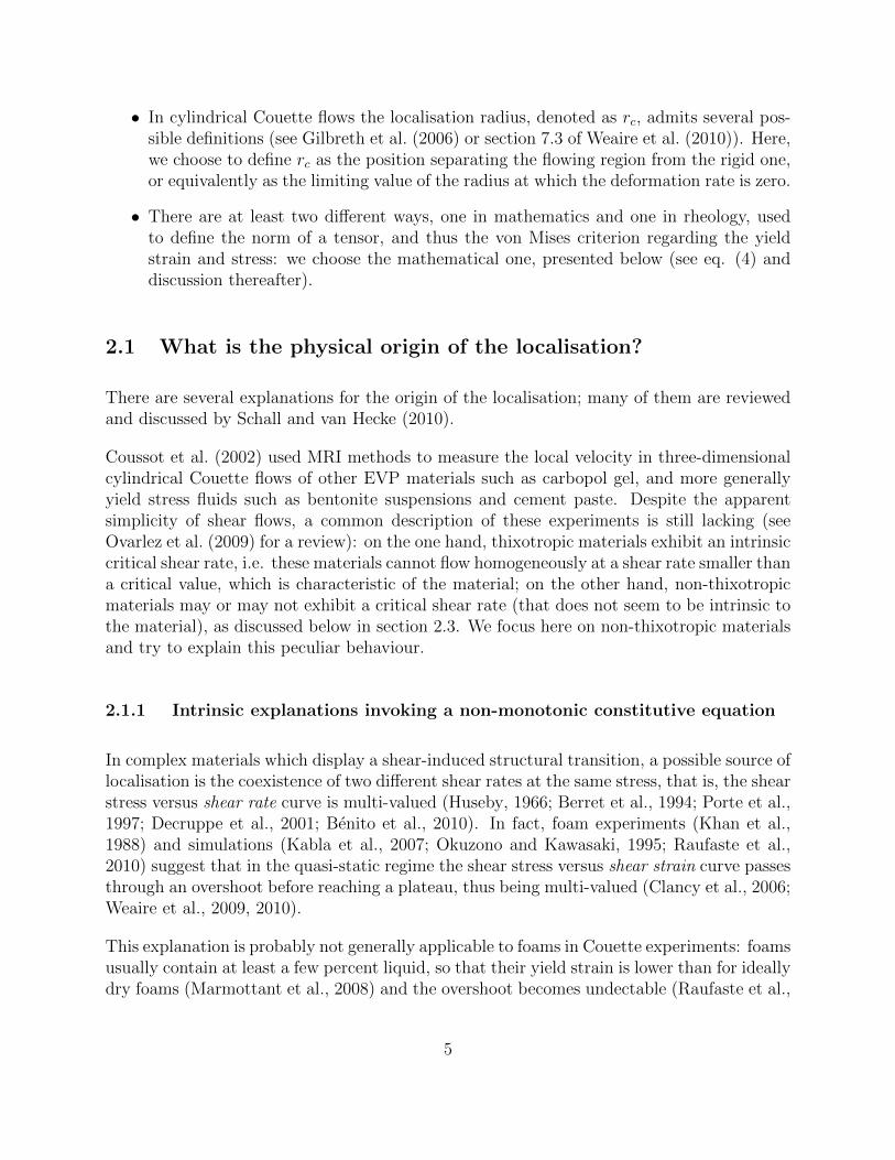
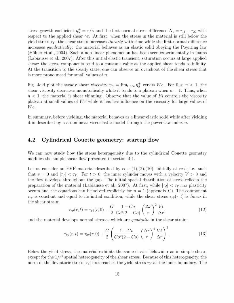
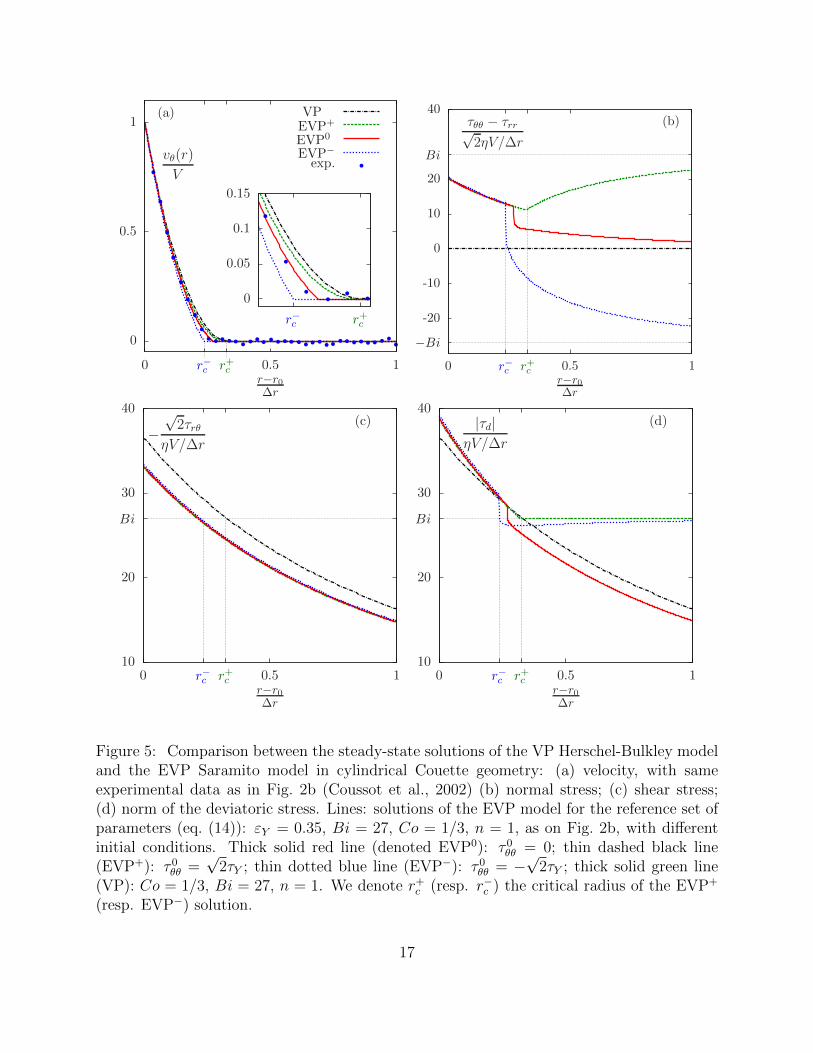
We now review some of the new insights gained from the tensorial EVP model, with anemphasis on the differences with scalar and/or VP models. Fig. 5 shows all the componentsof some solutions of the EVP model, for a set of parameters used as reference (eq. (14) andFig. 2b), and compares them to the VP model. The exploration of these parameters willbe presented in section 5. We define the critical shear rate γc as the jump of γ = 2Drθ atr = rc: it is visible as the slope of the velocity profile (see for instance Fig. 5a).

4.3.1 Range of possible initial conditions

The EVP constitutive equation (10) includes derivatives of the elastic stress tensor with re-spect to time and therefore allows the study of transient flows, as has been done by Cheddadiet al. (2008). This in turn requires to specify an initial condition that reflects the prepa-ration of the material before the beginning of the experiment. In particular, the tensorialframework allows us to study various initial normal stresses.

Three different constant values for τθθ are chosen. We denote by EVP0 the case where thecomponents of the initial stress are all set to zero. We then explore two limit cases, in whichthe component τθθ is such that the norm of the initial deviatoric stress tensor is |τd(r, θ, t=0)| = τY , while the other stress components are zero τrθ(r, θ, t=0) = τrr(r, θ, t=0) = 0. Wethus introduce the two cases EVP± corresponding to initial stresses τθθ(r, θ, t=0) = ±

√2τY .

Note that the component τrr(r, θ, t) remains constant and equal to its initial value zero in thecylindrical Couette geometry (see eq.(10)). We denote by r+

c (resp. r−c ) the critical radiuscorresponding to EVP+ (resp. EVP−).

4.3.2 Results

The results from the EVP model are dramatically different to the results from the VP model,for which the (steady-state) velocity is unique, the normal stress components are zero andthe localisation length rc is also unique for a given set of its parameters.

16

0

0.5

1

0 r−c r+c 0.5 1r−r0∆r

vθ(r)

V

(a)

0

0.05

0.1

0.15

r−c r+c

VPEVP+

EVP0

EVP−exp.

−Bi

-20

-10

0

10

20

Bi

40

0 r−c r+c 0.5 1r−r0∆r

τθθ − τrr√2ηV/∆r

(b)

10

20

Bi

30

40

0 r−c r+c 0.5 1r−r0∆r

−√2τrθ

ηV/∆r

(c)

10

20

Bi

30

40

0 r−c r+c 0.5 1r−r0∆r

|τd|ηV/∆r

(d)

Figure 5: Comparison between the steady-state solutions of the VP Herschel-Bulkley modeland the EVP Saramito model in cylindrical Couette geometry: (a) velocity, with sameexperimental data as in Fig. 2b (Coussot et al., 2002) (b) normal stress; (c) shear stress;(d) norm of the deviatoric stress. Lines: solutions of the EVP model for the reference set ofparameters (eq. (14)): εY = 0.35, Bi = 27, Co = 1/3, n = 1, as on Fig. 2b, with differentinitial conditions. Thick solid red line (denoted EVP0): τ 0

θθ = 0; thin dashed black line(EVP+): τ 0

θθ =√

2τY ; thin dotted blue line (EVP−): τ 0θθ = −

√2τY ; thick solid green line

(VP): Co = 1/3, Bi = 27, n = 1. We denote r+c (resp. r−c ) the critical radius of the EVP+

(resp. EVP−) solution.

17

Effect of the initial conditions. Surprisingly, Fig. 5 shows that the steady-state solutiondepends on the initial conditions. We find that they lead to three different steady-statesolutions, both for the velocity profile (Fig. 5a) and for the stress (Fig. 5b-d). For a givenset of parameters (εY , Bi, Co, n), when the initial condition varies the EVP model predictsa continuous set of steady-state solutions.

Non-uniqueness of the localisation length. Depending on the initial condition, thecritical radius rc can reach any value in the range [r−c , r

+c ]; the highest critical shear rate is

reached for the solution with EVP−. We find that r+c = r0 + 0.33∆r is close to the value

predicted by the VP model, but r−c = r0 + 0.24∆r is significantly smaller, while the criticalradius r0

c = r0 + 0.28∆r for EVP0 is in between.

Memory effects. Unlike the VP model, the EVP model exhibits non-zero normal stresses(Fig. 5b): in the flowing region (r < rc) where plastic rearrangements occur continuously(|τd| > τY ), the normal stress is independent of the initial conditions, and the materialprogressively loses memory of the initial condition. Conversely, in the non-flowing region(r > rc and |τd| < τY ), the normal stress depends strongly on the initial conditions. Thematerial thus keeps a record of the initial conditions through residual normal stresses.

Smooth and non-smooth solutions. Unlike the VP model, the EVP model can exhibiteither smooth (EVP+), or non-smooth profiles (EVP0, EVP−): the velocity gradient and thenormal stress can be discontinuous at r = rc (Fig. 5a). Compared to EVP0, EVP− exhibits astronger localisation (r−c < r0

c ), a higher γc, and a higher jump of the normal stress (Fig. 5b).

4.3.3 Comment on the non-uniqueness of the steady-state solutions

First, we point out that, for each given initial condition, the corresponding time-dependentproblem is well-posed, its time-dependent solution is unique, and the associated steady-statesolution is unique too. Let us then analyse the sources of the non-uniqueness of the solution.

First, from a qualitative point of view, the non-uniqueness of the steady-state solution canbe related to the transient elastic regime: in the extreme EVP− case, the component τθθstarts with a negative value that quadratically evolves with time (eq. (13)); meanwhile, theshear stress develops throughout the gap (eq. (12)), and as its contribution to the von Misescriterion dominates that of the normal stresses (see eq. (4) and Figs. 5b,c), the yield stressvalue τY is reached while the normal stresses are still negative. In the flowing region nearthe inner cylinder, the plastic term is not zero anymore and strongly couples the componentof the normal stresses to the flow. Their value is prescribed by the flow and no longerdepends on the initial condition in the flowing region (Fig. 5b); it differs from the non-flowing region where the normal stresses profiles strongly depend on the initial condition.When the steady-state regime is reached, these two regions do not join up, which resultsin discontinuous normal stresses and shear rate. The jump decreases as the initial stress is

18

increased (solutions EVP0 and EVP+, Fig. 5).

Second, from a formal point of view, the VP model (eq. (3)) contains one non-linearity,related to the von Mises criterion. The EVP model (eq. (10)) adds a second nonlinear-ity contained in the Oldroyd derivative (eq. (8)). Due to the expression of this Oldroydderivative, the steady-state EVP equations do not reduce to the VP model. The additionalterm couples the normal stresses components with the shear stress and the velocity gradient(appendix D). Therefore, even though the velocity gradient reduces here to the shear com-ponent, the EVP steady-state solution develops non-zero normal stresses. This additionalnonlinearity, interacting with the von Mises criterion, causes non-uniqueness of the stressesin the vicinity of |τd| = τY , i.e. in the vicinity of r = rc.

4.4 Comparison with experiments

We explain here how the parameters of the EVP model were chosen in order to fit theexperimental data shown in Fig. 2.

4.4.1 Smooth velocity profiles: the Debregeas et al. experiment

In the foam experiment shown in Fig. 2a, image analysis was used to find the steady-statevelocity profiles Debregeas et al. (2001); it was reanalysed by Janiaud and Graner (2005) whomeasured the shear and normal components of the local elastic strain, in both the transientand steady-state regime.

In the experiment, a steady state is reached after a transient regime. The rotation directionis then inverted, and after a second transient another steady state is reached: this is whenmeasurements are recorded (Debregeas et al., 2001). To perform a comparison, we use theexperimental steady state as an initial condition, invert the rotation, compute the numericalsolution until a first steady state is reached, then again invert the rotation, and compare thecorresponding steady state with experiments.

The value of the curvature number is fixed by the geometry:

Co = 1− r0

re= 1− 71

122≈ 0.41803.

We have to adjust the value of the three remaining parameters: εY , Bi, n. We focus on thesteady-state measurements of elastic strain and velocity.

We start with the yield strain εY ; this parameter is independent of the velocity and exerts alarge effect on the elastic strain ε(e) = τrθ/(2G) (see Cheddadi et al. (2011b)). We find thatεY = 0.175 allows a good fit of the measured value of the shear elastic strain (Fig. 6a). The

19

0

0.1

εY0.2

0.3

0 rc 0.5 1r−r0∆r

τ

2G

(a)

τrθ/(√2G) exp.

EVPd

τθθ/(2√2G) exp.

EVPd

τrr/(2√2G) exp.

EVPd

0

0.1

εY0.2

0.3

0 rc 0.5 1r−r0∆r

|τd|2G

(b)

exp.EVPd

Figure 6: The stress tensor: comparison of computations and experiments: (a) components;(b) norm of the tensor. Lines: computations with εY = 0.175, Bi = 10, Co = 0.41803,n = 1/3. Symbols: experiments (Debregeas et al., 2001) analysed by Janiaud and Graner(2005); errors bars have been provided by E. Janiaud (private communication).

initial normal components of the strain are not affected (Fig. 6b) by the successive rotationsin the region r > rc, and remain below the yield strain εY : this region undergoes reversibleelastic deformation.

Then we have to adjust the values of Bi and n. These parameters have much less effect thanεY on the profiles of ε(e), but they do affect the localisation length and the smoothness of thesolution (see Cheddadi et al. (2011b)). As this experiment exhibits a very smooth transitionfrom the flowing to the non-flowing region (exponential-like decrease of the velocity), oursensitivity analysis (see below, section 5.4) yields a good agreement with the data when usinga small value of the power-law index, n = 1/3.

The localisation length can be measured from the experiment: rc − r0 ≈ 0.3 ∆r; we canuse this information in the EVP model, taking advantage of the fact that the localisation isa VP effect and is mostly determined by the underlying VP model. This last model yieldsa relation between the values of rc, Bi, and n (see appendix A, equation (16)): with thechosen value of Co and n = 1/3, it yields Bi ≈ 7.6. This value is slightly adjusted in theEVP model in order to improve the fit: we obtain a better fit of the velocity profile withBi = 10.

20

4.4.2 Non-smooth profiles: the Coussot et al. experiment

The experiment shown in Fig. 2b was made with a bentonite-water suspension, usingMRI (Coussot et al., 2002). MRI measurements provide a precise and sharp velocity profilethat could not be obtained with foams (section 6.1). We use it here to explore the solutionsof the EVP model, without claiming to explain the particular properties of bentonite (whichis thixotropic) or any other specific material.

For this experiment, only the steady-state velocity has been measured, which makes it moredifficult to evaluate precisely the parameters of the EVP model. Since the normal stressesare not measured, we take an initial condition set to zero for the sake of simplicity. As thevelocity profile is quite abrupt in the vicinity of r = rc, we choose n = 1 for the power-lawindex. Then, as for the previous experiment, we evaluate the Bingham number Bi under thecondition that the critical radius predicted by the underlying VP model matches the valuein the experiment (rc−r0 = 0.28 ∆r). From this point, the slope of velocity at r = rc (whichis directly related to the critical shear rate) can be adjusted by tuning the yield strain εY .The best fit is obtained with εY = 0.35 and Bi = 27.

5 Sensitivity to the parameters

Now, we study how the range [r−c , r+c ] and the critical shear rate γc depend on the param-

eters of the EVP model. We explore the parameter space with the dimensionless numbers(εY , Bi, Co, n). It allows us to probe the effect of the imposed velocity V , through the Bing-ham number, as it is the only one that depends on V ; the geometry, through the curvaturenumber Co; and the two material parameters: the yield strain εY , and the power-law indexn. These parameters are varied around a reference set of parameters used for the comparisonwith Coussot et al. (2002) (section 4.4.2, Fig. 2b):

εY = 0.35, Bi = 27, n = 1, Co = 1/3. (14)

5.1 Effect of the inner cylinder velocity V

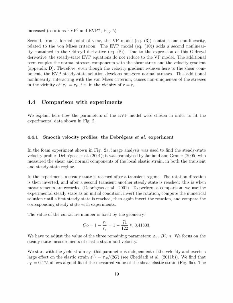
The effect of the imposed velocity V is probed through Bi, which is varied in the range[10, 60] around the reference value Bi = 27. If V0 is the velocity associated with this referencevalue, the range of Bi corresponds roughly to the range [V0/3, 3V0] for the velocity. Observeon Fig. 7a that when the Bingham number Bi increases then rc decreases and the size ofthe zero-velocity zone increases. The critical radius r+

c almost matches the critical radiuspredicted by the VP model. The flow becomes more localised and the gap between r−c andr+c also decreases slowly. The marker represents our reference solution (on Fig. 7a). We

21

0

0.25

0.5

0 25 50

Bi

r±c − r0∆r

(a)

0

1

2

3

4

5

0 25 50

Bi

−∆r

V0γc

(b)

Figure 7: Effect of the Bingham number Bi. (a) r−c and r+c . Red bars: five examples of the

range in which (rc−r0)/δr varies. Black cross: parameters as (14) together with τ(t=0) = 0.Solid black line: value predicted by the VP model with the same parameters except thatεY = 0. From Coussot et al. (2002) we get V0/∆r = 0.67 s−1. (b) Corresponding values ofγc.

observe on Fig. 7b that γc is almost constant when Bi varies. Varying the velocity affectsthe size of the zero-velocity zone, but has little effect upon the possible abruptness of thesolution, nor on the range [r−c , r

+c ].

5.2 Effect of the curvature Co

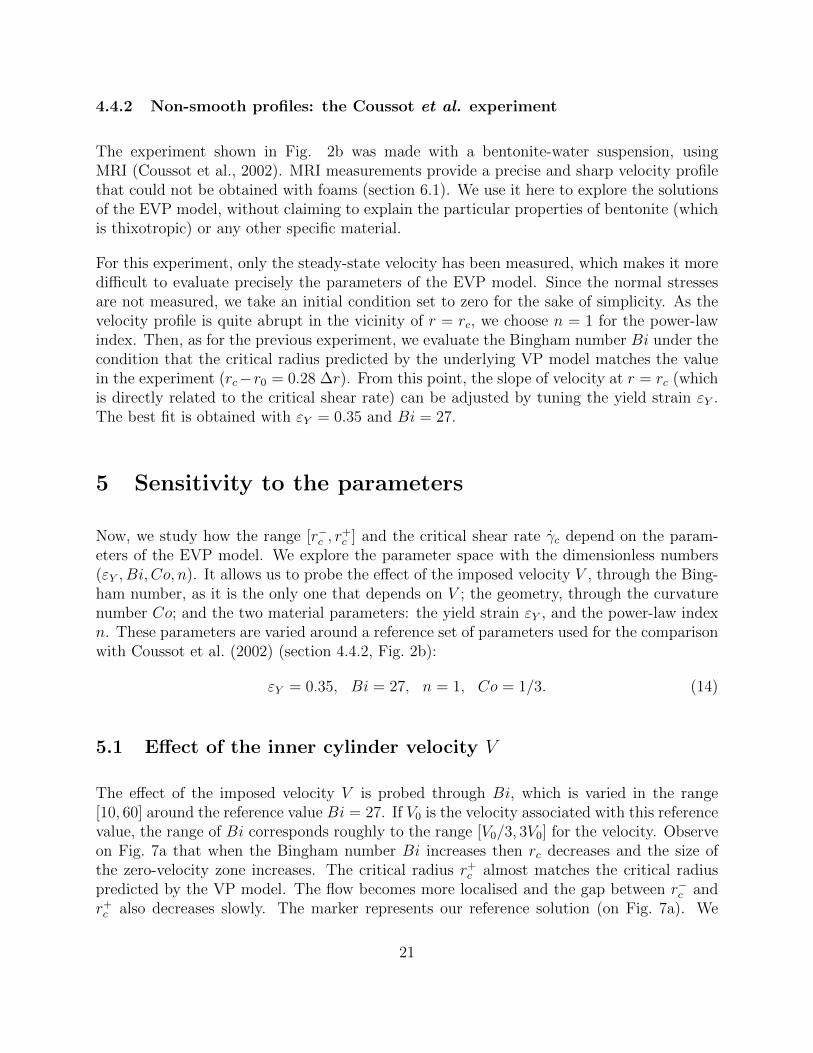
The curvature number Co explores the effect of the curvature of the geometry. Recall thatCo → 0 corresponds to the plane Couette, with a homogeneous stress throughout the gap,while Co close to one corresponds to cylindrical Couette with a tiny central cylinder, anda highly heterogeneous stress. Observe on Fig. 8 that the size of the zero-velocity zonedecreases when Co tends to one. The critical radius r+

c of the smooth solution is wellpredicted by the VP model. Note also that the difference r+

c − r−c decreases with Co: thus,when rc is close to r0, the effect of the initial condition on the localisation length is lessvisible. Also the maximal discontinuity γc of the critical shear rate increases with Co.

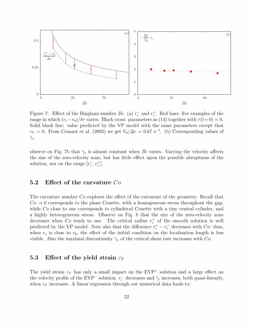
5.3 Effect of the yield strain εY

The yield strain εY has only a small impact on the EVP+ solution and a large effect onthe velocity profile of the EVP− solution: r−c decreases and γc increases, both quasi-linearly,when εY increases. A linear regression through our numerical data leads to:

22

0

0.25

0.5

0 110

13

12

34

910

1

Co

r±c − r0∆r

(a)

0

1

2

3

4

5

6

7

0 110

13

12

34

910

1

Co

−∆r

Vγc

(b)

Figure 8: Effect of the curvature Co: same caption as Fig. 7.

r−c − r0

∆r≈ −0.23 εY + 0.33

−∆r

Vγc ≈ 5.5 εY . (15)

Note that both the range r+c − r−c and the discontinuity γc increase with εY . Accordingly,

when εY vanishes, r−c = r−c and γc = 0: the solution is unique and smooth: there is noelasticity and the model reduces to the VP one.

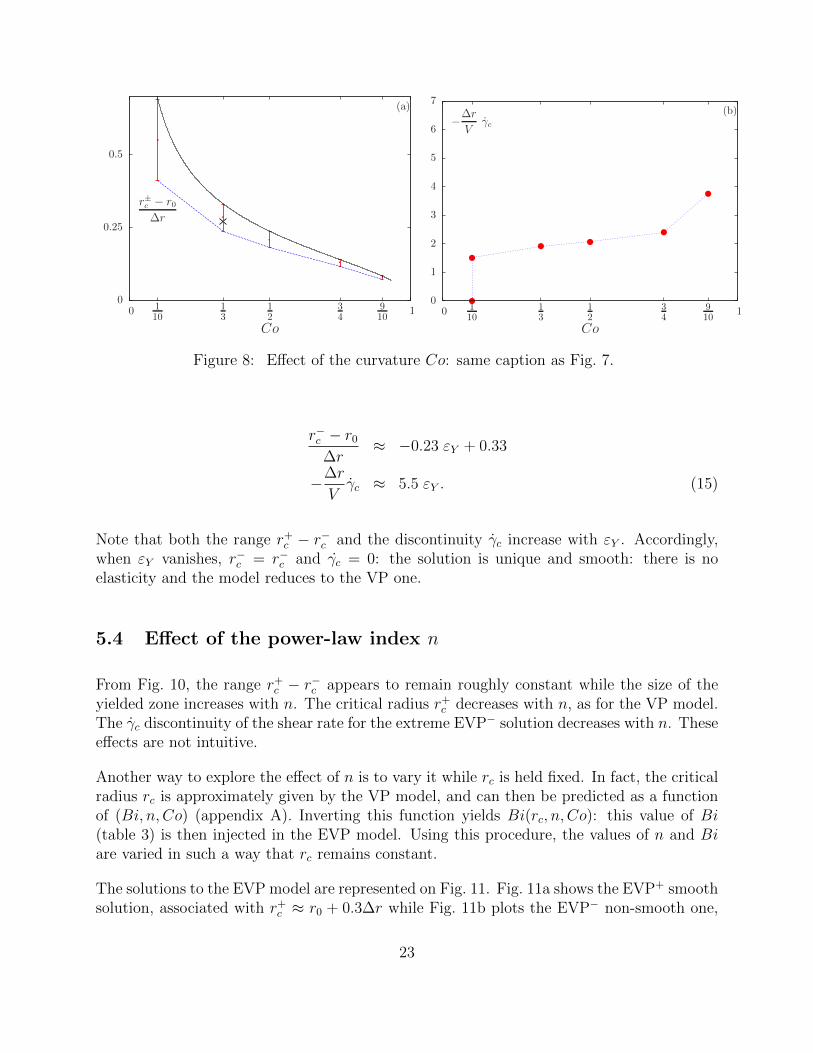
5.4 Effect of the power-law index n

From Fig. 10, the range r+c − r−c appears to remain roughly constant while the size of the

yielded zone increases with n. The critical radius r+c decreases with n, as for the VP model.

The γc discontinuity of the shear rate for the extreme EVP− solution decreases with n. Theseeffects are not intuitive.

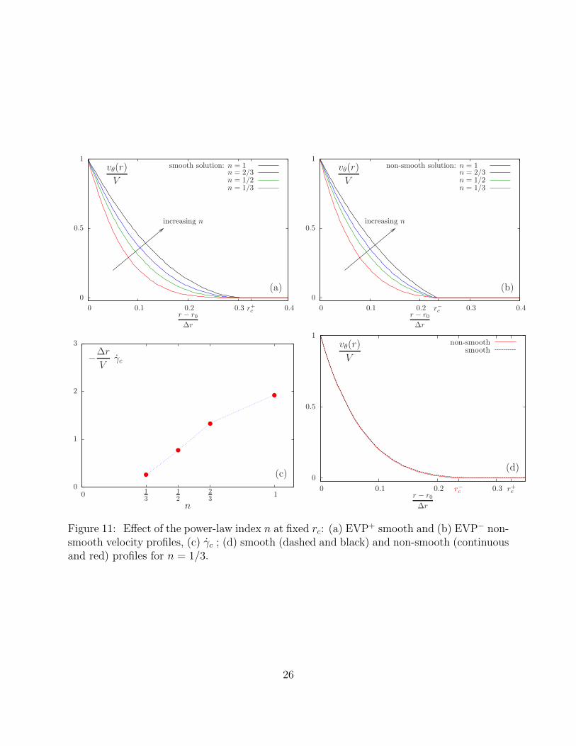
Another way to explore the effect of n is to vary it while rc is held fixed. In fact, the criticalradius rc is approximately given by the VP model, and can then be predicted as a functionof (Bi, n, Co) (appendix A). Inverting this function yields Bi(rc, n, Co): this value of Bi(table 3) is then injected in the EVP model. Using this procedure, the values of n and Biare varied in such a way that rc remains constant.

The solutions to the EVP model are represented on Fig. 11. Fig. 11a shows the EVP+ smoothsolution, associated with r+

c ≈ r0 + 0.3∆r while Fig. 11b plots the EVP− non-smooth one,

23

0

0.25

0.5

0 0.5 1

εY

r±c − r0∆r

(a)

0

1

2

3

4

5

0 0.5 1

εY

−∆r

Vγc

(b)

Figure 9: Effect of the yield strain εY : same caption as Fig. 7. Dashed lines: fits of theEVP− solutions to the data.

n 1/3 1/2 2/3 1Bi 9.54785 12.7851 16.6489 27

Table 3: Effect of the power-law index n while rc remains fixed: values of n and correspondingvalues of Bi (εY = 0.35, Co = 1/3).

with r−c ≈ r0 + 0.23∆r. Note that both r+c and r−c are now roughly constant, and that the

velocity profile is more curved when n is small.

Fig. 11c shows γc: observe that the discontinuity decreases rapidly when n decreases. Forn = 1/3, the non-smoothness becomes imperceptible, while the EVP+ smooth and EVP−

non-smooth profiles are very close and almost indiscernable, as shown on Fig. 11d. Notethat even when n = 1/3, there are still multiple solutions, and the range for rc remains aslarge as [r−c − r0, r

+c − r0] ≈ [0.23, 0.3]∆r, despite the fact that these solutions share similar

curved profiles.

6 Discussion

6.1 Smooth and non-smooth profiles

The debate about smooth and non-smooth velocity profiles, mentioned in the introduction,is difficult to address experimentally, for two reasons.

24

0

0.25

0.5

0 13

12

23

1

n

r±c − r0∆r

(a)

0

1

2

3

4

5

6

7

0 13

12

23

1

n

−∆r

Vγc

(b)

Figure 10: Effect of the power-law index n: same caption as Fig. 7.

First, since the steady-state solution is not unique, both smooth and non-smooth profilescan be observed in the same experiment. This depends on the residual stresses due tothe initial preparation, which are usually not reproducible and are certainly difficult tosuppress (Labiausse et al., 2007; Raufaste et al., 2010), or on the presence of some impurities.This high sensitivity might explain some discrepancies in the literature, and the difficulty tosettle the debates regarding localisation.

Second, the experiments in foams are not always precise enough to discriminate betweensmooth and non-smooth transitions. Fig. 12 compares experimental measurements and thetwo solutions: EVP+, the smooth one, with dashed lines, and EVP−, the non-smooth one,with solid lines. Experiments were performed with bubble rafts, and in order to reflectthe absence of top and bottom plates, the fluid viscosity is introduced in computations asa second Newtonian viscosity η2 with a viscosity ratio α = η/(η + η2) (Saramito, 2007,2009). In that case, the smooth solution predicts r+

c = r0 + 0.65∆r and the non-smoothone r−c = r0 + 0.43∆r together with a critical shear rate γc = 0.33 V/∆r. Observe thatneither the smooth or the non-smooth solutions can be distinguished from the experimentalmeasurements.

6.2 Is Couette flow suitable for caracterizing EVP materials?

6.2.1 Flow geometry

We recommend to study flows where residual stresses do not affect the understanding andmeasurements. Other requirements should include: well-defined boundary conditions; a goodseparation of scale between the discrete units, the representative volume element (RVE) and

25

0

0.5

1

0 0.1 0.2 0.3 r+c 0.4r − r0∆r

vθ(r)

V

(a)

increasing n

smooth solution: n = 1n = 2/3n = 1/2n = 1/3

0

0.5

1

0 0.1 0.2 r−c 0.3 0.4r − r0∆r

vθ(r)

V

(b)

increasing n

non-smooth solution: n = 1n = 2/3n = 1/2n = 1/3

0

1

2

3

0 13

12

23

1

n

−∆r

Vγc

(c) 0

0.5

1

0 0.1 0.2 r−c 0.3 r+cr − r0∆r

vθ(r)

V

(d)

non-smoothsmooth

Figure 11: Effect of the power-law index n at fixed rc: (a) EVP+ smooth and (b) EVP− non-smooth velocity profiles, (c) γc ; (d) smooth (dashed and black) and non-smooth (continuousand red) profiles for n = 1/3.

26

0

0.5

1

0 0.2 0.4 0.6 0.8 1r−r0∆r

vθ(r)

Ωr

0.85

0.9

0.95

1

1.05

0.3 0.4 0.5 0.6

exp.EVP− solutionEVP+ solution

Figure 12: Foam showing abrupt velocity profile. Comparison of experimental data,from Gilbreth et al. (2006), Fig. 1, with model (εY = 0.2, Bi = 1.3, Co = 0.63333, n = 1,α = 0.2) for both smooth EVP+ and non-smooth EVP− (τθθ(t=0) = ±

√2Bi) solutions.

27

the global flow scale; the possibility to have a large variation of the control parameters such asvelocity (and in foams, liquid fraction and bubble size dispersity); a variety of measurementsproviding stringent tests on the EVP model and its parameters. We have shown usingexperiments and models that a foam flow around an obstacle (Stokes flow) meets theserequirements (Cheddadi et al., 2011a).

Couette flows, due to their simple geometry, have a long history of being used to probe therheology of Newtonian fluids. They are also suitable for complex liquids such as VE or VPmaterials. However, the present study questions their use in EVP materials, and especiallyin foams, which are usually excellent model materials to perform in-lab experiments. In fact,in EVP materials, the initial conditions and the preparation method create residual stresseswhich are difficult to remove and affect the flow, which thus becomes non-unique and poorlycontrolled. Care is necessary to interpret the results. Future experimental work could tryto deepen our understanding of localisation and to test our predictions by working in thefollowing two directions.

6.2.2 Sample preparation

The control of the sample preparation, and of the initial normal stresses, is important.Obtaining different (although uncontrolled) initial conditions should be reasonably easy bytrying different methods to fill the experimental cell.

Choosing these initial stresses is less easy, but possible for instance by performing a highvelocity pre-shear in the reverse direction. If the shear rate is high enough so that nolocalisation is observed in the steady-state regime, the normal stresses reach a value largerthan

√2τY . Whatever the initial loading of the material, it has been irreversibly erased

by the plastic rearrangements. After such a pre-shear, one should observe smooth velocityprofiles, with no critical shear rate. We have numerically checked that after such a highvelocity pre-shear the EVP model predicts a smooth solution (similar to EVP+), even withthe EVP− initial loading, that would lead without pre-shear to a non-smooth solution.

Suppressing these initial stresses is approximately (but not completely) possible by a carefulsample deposition in the experimental cell (Labiausse et al., 2007). Complete suppressionwould for instance require applying cycles of oscillating strain of amplitude which begins ataround twice the yield strain and then gradually decreases to zero (Raufaste et al., 2010);since these cycles have to be performed in each of the three dimensions, such suppression ofinitial stress would require a dedicated experiment and is in fact easier in simulations.

Finally, some coarsening materials such as foams become gradually isotropic with time, sothat their trapped stresses slowly decrease (Hohler and Cohen-Addad, 2005).

We emphasize the fact that these two last procedures tend to suppress normal stresses and

28

therefore correspond to the EVP0 initial loading and non-smooth solutions.

6.2.3 Measurements of parameters and variables

We recommend to perform local measurements of strain or stress. In situ measurementof strain is purely geometric and independent of any knowledge of the sample physics: itcan be performed on most systems where the positions of each discrete constituent objectis measurable (Graner et al., 2008), which includes two-dimensional foams (Janiaud andGraner, 2005; Marmottant et al., 2008) or colloids. In situ measurements of stresses arepossible with similar methods by measuring the positions of the discrete constituents andhaving some knowledge of their physical interactions, for instance in two-dimensional foams(Marmottant et al., 2008), or in birefringent materials by using photoelasticity (Miller et al.,1996).

Model parameters are all measurable in principle. Note that the yield strain or stress re-quires a tensorial measurement, and thus normal differences components (Labiausse et al.,2007). Again, local measurements of strain can help in measuring the yield strain directly(Marmottant et al., 2008).

7 Summary

We solve here a tensorial model for the cylindrical Couette flow of elastic, viscous, plasticmaterials. We provide an approximate expression for the rheology versus different materialparameters. In turn, our predictions are compared with experiments. We show that thereis a complex interplay between elasticity, viscosity and plasticity, which together (but notseparately) account for experimental observations. Even in such a simple geometry, the ori-entational effects are important, so that a tensorial EVP description is necessary to capturemany aspects of the physics: reversible elastic deformation (both shear and normal com-ponents) below τY , following the Poynting law; memory of the preparation of the materialthrough the initial stress condition, and consequently non-uniqueness of the steady flow andpersistent residual normal stresses; possible appearance of non-smooth solutions. The nor-mal stresses can be interpreted as an intrinsic structure parameter at the macroscopic level,and therefore independent of the underlying microstructure. These features can be predictedneither by VP models nor by VE models.

We have computed numerically the value of the localisation length versus different parametersso that we can guide experimentalists to design experiments that may or may not exhibitsuch effects: the effects of the initial conditions are more visible for instance when εY is large;or when the dissipation exponent n is large; or when the velocity is large, but small enough

29

to allow for a localisation within the gap; or when the heterogeneity from the geometry issmall, but large enough to allow for a localisation within the gap.

Altogether, our results provide a validation of the continuous material description, a de-termination of EVP material parameters, and an in-depth understanding of their complexrheology. Finally, it appears that the steady Couette flow, which has stimulated so manydebates, is neither robust nor unique. Despite its apparent simplicity, it involves numerousparameters, such as the initial conditions for the stress tensor, and is difficult to use in prac-tice. Couette flow experiments could be complemented with flows in other geometries, witha stronger dependence in time and/or space.

Acknowledgements

We warmly thank S. Cox and G. Ovarlez for detailed comments on the manuscript, M.Dennin and E. Janiaud for providing data, S. Cohen-Addad, B. Dollet and C. Gay forfruitful discussions, the French Groupe de Recherches “Mousses et Emulsions”, C. Gay andC. Philippe-Barache for funding the travels for collaborations. FG thanks D. Weaire forintense discussions and questions which stimulated this work.

30

References

J. M. Adams and P. D. Olmsted. Nonmonotonic models are not necessary to obtain shearbanding phenomena in entangled polymer solutions. Phys. Rev. Lett., 10:067801, 2009.

J. D. Barry, D. Weaire, and S. Hutzler. Nonlocal effects in the continuum theory of shearlocalisation in 2d foams. Phil. Mag. Lett., 91:432–440, 2011.

S. Benito, C.-H. Bruneau, T. Colin, C. Gay, and F. Molino. An elasto-visco-plastic modelfor immortal foams or emulsions. Eur. Phys. J. E, 25:225–251, 2008.

S. Benito, F. Molino, C.-H. Bruneau, T. Colin, and C. Gay. Shear bands in a continuummodel of foams: how a 3d homogeneous material may seem inhomogeneous in 2d. preprint,2010. URL http://arxiv.org/abs/1011.0521.

J.-F. Berret, D. C. Roux, and G. Porte. Isotropic-to-nematic transition in wormlike micellesunder shear. Europ. Phys. Journal E, 4:1261–1279, 1994.

E. C. Bingham. Fluidity and plasticity. Mc Graw-Hill, New-York, USA, 1922.

I. Cantat, S. Cohen-Addad, F. Elias, F. Graner, R. Hohler, O. Pitois, F. Rouyer, andA. Saint-Jalmes. Les mousses: structure et dynamique. Belin, Paris, 2010.

I. Cheddadi, P. Saramito, C. Raufaste, P. Marmottant, and F. Graner. Numerical modellingof foam Couette flows. Eur. Phys. J. E, 27:123–133, 2008.

I. Cheddadi, P. Saramito, C. Raufaste, P. Marmottant, and F. Graner. Erratum to numericalmodelling of foam Couette flows. Eur. Phys. J. E, 28:479–480, 2009.

I. Cheddadi, P. Saramito, B. Dollet, C. Raufaste, and F. Graner. Understanding and pre-dicting viscous, elastic, plastic flows. Eur. Phys. J. E. Soft matter, 34:11001, 2011a.

I. Cheddadi, P. Saramito, and F. Graner. Stationary Couette flows of elastoviscoplastic fluids(supplementary information), 2011b. [URL will be inserted by AIP].

R. J. Clancy, E. Janiaud, D. Weaire, and S. Hutzler. The response of 2D foams to continuousapplied shear in a Couette rheometer. Eur. Phys. J. E, 21:123–132, 2006.

P. Coussot and G. Ovarlez. Physical origin of shear-banding in jammed systems. Eur. Phys.J. E, 33:183–188, 2010.

P. Coussot, J. S. Raynaud, F. Bertrand, P. Moucheront, J. P. Guilbaud, H. T. Huynh,S. Jarny, and D. Lesueur. Coexistence of liquid and solid phases in flowing soft-glassymaterials. Phys. Rev. Lett., 88:218301, 2002.

F. da Cruz, F. Chevoir, D. Bonn, and P. Coussot. Viscosity bifurcation in granular materials,foams, and emulsion. Phys. Rev. E, 66:051305, 2002.

31

G. Debregeas, H. Tabuteau, and J.-M di Meglio. Deformation and flow of a two-dimensionalfoam under continuous shear. Phys. Rev. Lett., 87:178305, 2001.

J. P. Decruppe, S. Lerouge, and J.-F. Berret. Insight in shear banding under transient flow.Phys. Rev. E, 63:022501, 2001.

N. D. Denkov, S. Tcholakova, K. Golemanov, and A. Lips. Jamming in sheared foams andemulsions, explained by critical instability of the films between neighboring bubbles anddrops. Phys. Rev. Lett., 103:118302, 2009.

M. Dennin. Discontinuous jamming transitions in soft materials: coexistence of flowing andjammed states. J. Phys.: Condens. Matter, 20:283103, 2008.

D. Doraiswamy, A. N. Mujumdar, I. Tsao, A. N. Beris, S. C. Danforth, and A. B. Metzner.The Cox-Merz rule extended: a rheological model for concentrated suspensions and othermaterials with a yield stress. J. Rheol., 35:647–685, 1991.

C. Gilbreth, S. Sullivan, and M. Dennin. Flow transition in two-dimensional foams. Phys.Rev. E, 74:031401, 2006.

F. Graner, B. Dollet, C. Raufaste, and P. Marmottant. Discrete rearranging disorderedpatterns, part I: robust statistical tools in two or three dimensions. Eur. Phys. J. E, 25:349–369, 2008.

W. H. Herschel and T. Bulkley. Measurement of consistency as applied to rubber-benzenesolutions. Proceedings of the American Society for Testing and Material, 26:621–633, 1926.

R. Hohler and S. Cohen-Addad. Rheology of liquid foam. J. Phys. Condens. Matt., 17(41):R1041, 2005.

R. Hohler, S. Cohen-Addad, and V. Labiausse. A constitutive equation describing the nonlin-ear elastic response of aqueous foams and concentrated emulsions. J. Rheol., 48:679–690,2004.

D. Howell, R. P. Behringer, and C. Veje. Stress fluctuations in a 2D granular Couetteexperiment: a continuous transition. Phys. Rev. Lett., 82:5241–5244, 1999.

N. Huang, G. Ovarlez, F. Bertrand, S. Rodts, P. Coussot, and D. Bonn. Flow of wet granularmaterials. Phys. Rev. Lett., 94:028301, 2005.

T. W. Huseby. Hypothesis on a certain flow instability in polymer melts. Trans. Soc. Rheol.,10:181, 1966.

A. I. Isayev and X. Fan. Viscoelastic plastic constitutive equation for flow of particle filledpolymers. J. Rheol., 34:35–54, 1990.

E. Janiaud and F. Graner. Foam in a two-dimensional Couette shear: a local measurementof bubble deformation. J. Fluid Mech., 532:243–267, 2005.

32

E. Janiaud, D. Weaire, and S. Hutzler. Two-dimensional foam rheology with viscous drag.Phys. Rev. Lett., 97:038302, 2006.

A. Kabla, J. Scheibert, and G. Debregeas. Quasistatic rheology of foams I. Oscillating strain.J. Fluid Mech., 587:23–44, 2007.

G. Katgert, M. E. Mobius, and M. van Hecke. Rate dependence and role of disorder inlinearly sheared two-dimensional foams. Phys. Rev. Lett., 101:058301, 2008.

G. Katgert, A. Latka, M. E. Mobius, and M. van Hecke. Flow in linearly sheared two-dimensional foams: From bubble to bulk scale. Phys. Rev. E, 79:066318, 2009.

G. Katgert, B. P. Tighe, M. E. Mobius, and M. M. van Hecke. Couette flow of two-dimensional foams. Europhys. Lett., 90:54002, 2010.

S. A. Khan, C. A. Schnepper, and R. C. Armstrong. Foam rheology: III. Measurement ofshear flow properties. J. Rheol., 32:69–92, 1988.

K. Krishan and M. Dennin. Viscous shear banding in foam. Phys. Rev. E, 78:051504, 2008.

V. Labiausse, R. Hohler, and S. Cohen-Addad. Shear induced normal stress differences inaqueous foams. J. Rheol., 51:479–492, 2007.

J. Lauridsen, G. Chanan, and M. Dennin. Velocity profiles in slowly sheared bubble rafts.Phys. Rev. Lett., 93(1):018303, 2004.

W. Losert, L. Bocquet, T. C. Lubensky, and J. P. Gollub. Particle dynamics in shearedgranular matter. Phys. Rev. Lett., 85:1428–1431, 2000.

P. Marmottant, C. Raufaste, and F. Graner. Discrete rearranging disordered patterns, partII: 2D plasticity, elasticity and flow of a foam. Eur. Phys. J. E, 25:371–384, 2008.

B. Miller, C. O’Hern, and R. P. Behringer. Stress fluctuations for continuously shearedgranular materials. Phys. Rev. Lett., 77:3110, 1996.

D. M. Mueth, G. F. Debregeas, G. S. Karczmar, P. J. Eng, S. R. Nagel, and H. M. Jaeger.Signatures of granular microstructure in dense shear flows. Nature, 406:385–389, 2000.

T. Okuzono and K. Kawasaki. Intermittent flow behavior of random foams: a computerexperiment on foam rheology. Phys. Rev. E, 51:1246–1253, 1995.

J. G. Oldroyd. A rational formulation of the equations of plastic flow for a Bingham fluid.Proc. Cambridge Philos. Soc., 43:100–105, 1947.

J. G. Oldroyd. On the formulation of rheological equations of states. Proc. Roy. Soc. LondonA, 200:523–541, 1950.

33

G. Ovarlez, S. Rodts, X. Chateau, and P. Coussot. Phenomenology and physical origin ofshear localization and shear banding in complex fluids. Rheol. Acta, 48:831–844, 2009.

G. Ovarlez, K. Krishan, and S. Cohen-Addad. Investigation of shear banding in three-dimensional foams. Europhys. Lett., 91:68005, 2010.

G. Porte, J.-F. Berret, and J. Harden. Inhomogeneous flows of complex fluids: mechanicalinstability versus non-equilibrium phase transition. Eur. Phys. J. E, 7:459–472, 1997.

A. M. Puzrin, A. M. Asce, and G. T. Houlsby. Rate-dependent hyperplasticity with internalfunctions. Journal of Engineering Mechanics, 129:252–263, 2003.

C. Raufaste, S. J. Cox, P. Marmottant, and F. Graner. Discrete rearranging disorderedpatterns: prediction of elastic and plastic behavior, and application to two-dimensionalfoams. Phys. Rev. E, 81:031404, 2010.

S. Rodts, J. C. Baudez, and P. Coussot. From discrete to continuum flow in foams. Europhys.Lett., 69:636–642, 2005.

J.-B. Salmon, A. Colin, S. Manneville, and F. Molino. Velocity profiles in shear-bandingwormlike micelles. Phys. Rev. Lett., 90:228303, 2003a.

J.-B. Salmon, S. Manneville, and A. Colin. Shear banding in a lyotropic lamellar phase. ii.temporal fluctuations. Phys. Rev. E, 68:051504, 2003b.

P. Saramito. A new constitutive equation for elastoviscoplastic fluid flows. J. Non NewtonianFluid Mech., 145:1–14, 2007.

P. Saramito. A new elastoviscoplastic model based on the Herschel-Bulkley viscoplasticity.J. Non Newtonian Fluid Mech., 158:154–161, 2009.

P. Saramito. Efficient C++ finite element computing with Rheolef. CNRS and LJK,2011. URL http://www-ljk.imag.fr/membres/Pierre.Saramito/rheolef/rheolef.

pdf. http://www-ljk.imag.fr/membres/Pierre.Saramito/rheolef/rheolef.pdf.

P. Schall and M. van Hecke. Shear bands in matter with granularity. Annu. Rev. FluidMech., 42:67–88, 2010.

T. Schwedoff. La rigidite des liquides. In Congres Int. Physique, Paris, volume 1, pages478–486, 1900.

J. Vermant. Large-scale structures in sheared colloidal dispersions. Curr. Opin. Coll. Int.Sci., 6:489–495, 2001.

Y. Wang, K. Krishan, and M. Dennin. Impact of boundaries on velocity profiles in bubblerafts. Phys. Rev. E, 73:031401, 2006.

D. Weaire and S. Hutzler. The physics of foam. Oxford University Press, UK, 1999.

34

D. Weaire, R. J Clancy, and S Hutzler. A simple analytical theory of localisation in 2d foamrheology. Philosophical Magazine Letters, 89:294–296, 2009.

D. Weaire, J. D. Barry, and S. Hutzler. The continuum theory of shear localization intwo-dimensional foam. J. Phys.: Condens. Matter, 22:193101, 2010.

A. Wyn, I. T. Davies, and S. J. Cox. Simulations of two-dimensional foam rheology: local-ization in linear Couette flow and the interaction of settling discs. Eur. Phys. J. E, 26:81–89, 2008.

35

A Herschel-Bulkley solution in cylindrical geometry

When εY = 0 the EVP model reduces to the VP one, and the velocity profile is given by

vθ(r) =

(√2 r2

c τYK

) 1n

r

∫ rc

r

1

s

(1

s2− 1

r2c

) 1n

ds

In the case where the flow is driven by the inner boundary, the critical radius rc is given bythe following expression:

τY =K√2 r2

c

v(r0)

r0

∫ rc

r0

1

s

(1

s2− 1

r2c

) 1n

ds

n

.

It expresses also in dimensionless variables:

Bi =√

2

(∆r

rc

)2 r0

∆r

∫ rc/∆r

r0/∆r

1

s

(1

s2−(

∆r

rc

)2) 1

n

ds

−n , (16)

For fixed values of n and rc, the corresponding value of Bi for the VP model, denoted asBivp(n, rc), can be easily computed by using numerical integration. Conversely, for given Biand n, the value of rc associated to the VP model, denoted as rvp

c (n,Bi), can be obtainedfrom a small numerical computation (Fig. 13a).

Fig. 13a plots rc as a function of the Bingham number Bi, for εY = 0 (VP model) andCo = 1/3, and different values of the power-law index n. Note that the value Co = 1/3corresponds to the geometry of the experiment by Coussot et al. (2002) as shown on Fig. 2b.In this geometry, the localisation is observed as long as rc/∆r < re/∆r = 1/Co. The VPmodel predicts that rc decreases with the Bingham number: the zero-velocity zone developsand the localisation effect is more pronounced. Observe also that the localisation effect ismore pronounced when n decreases at fixed values of Bi and Co. The rc value associated tothe VP model is denoted as rc,vp(n,Bi) and its inverse function as Bivp(n, rc). At fixed n,rc depends on Bi roughly as a power-law:

rc(Bi, n)− r0

∆r≈ 1.82Biβn . (17)

Fig. 13b represents βn vs n. A nonlinear regression leads to the dotted line of equation:

βn ≈ −0.38n2 + 0.88n− 1.02, (18)

36

10−3

10−2

10−1

1

1 10 102 103 104 105 106

Bi

rvpc (n,Bi)− r0∆r

n = 1n = 2/3n = 1/2n = 1/3

-1

-0.75

-0.5

13

12

23 1

n

βn

Figure 13: VP model (εY = 0, Co = 1/3): (a) localisation rc = rvpc (Bi, n) versus the

Bingham number Bi, for different values of the power-law index n ; (b) index βn vs n forthe power-law (rc(Bi, n)− r0)/∆r ≈ 1.82Biβn . Dotted line: eq. (18).

0

0.05

0.10

0.15

0.2 r−c 0.3r−r0∆r

vθ(r)

V

(a)

h/∆r = 1/8001/4001/2001/100

−Bi

-20

-10

0

10

20

Bi

0 r−c 0.5 1r−r0∆r

τθθ − τrr√2ηV/∆r

(b)

h/∆r = 1/8001/4001/2001/100

Figure 14: Convergence vs mesh refinement for the EVP− non-smooth solution (εY = 0.35,Bi = 27, Co = 1/3, n = 1) as on Fig. 5.

37

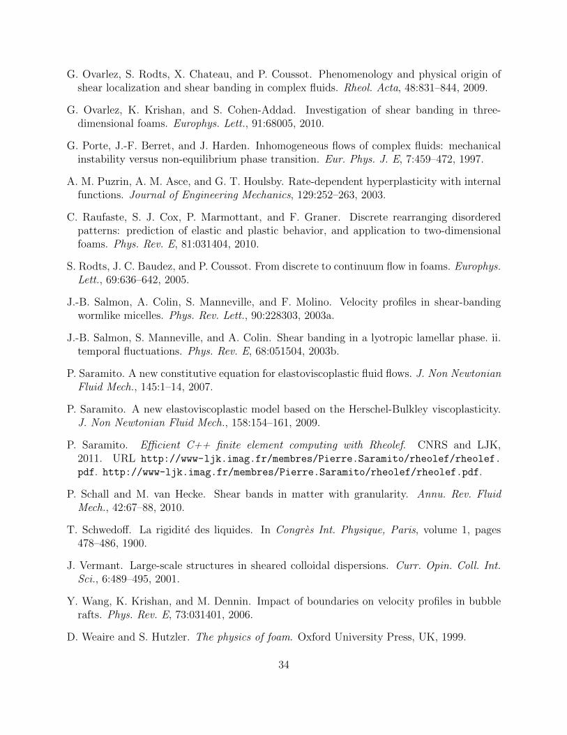
B Numerical method

The velocity is approximated by continuous affine finite elements while the stress componentsare piecewise constant over the mesh. The code is implemented by using the C + + Rheoleffinite element library (Saramito, 2011). The stopping criteria for a steady solution is satisfiedwhen the residual term is less than 10−8. Fig. 14 shows the convergence versus the mesh sizeh at the vicinity of r = rc for the EVP− non-smooth steady solution presented on Fig. 5.Observe that the numerical method presents excellent convergence properties, despite thenon-smoothness of the solution: the velocity is non-differentiable (Fig. 14a) while normalstress is discontinuous (Fig. 14b).

C Calculations for startup flow

The initial condition is such that v = 0 and |τd| < τY throughout the gap. For t > 0, theinner cylinder moves with a velocity V > 0. The calculations that follow are valid as longas no plasticity occurs.

Eq. (23) yields τrθ = −C(t)/r2, where C(t) depends only on time. With n = 1, eq. (19)yields τrr = 0 if we choose τrr(r, 0) = 0 in the initial condition. As a results, eq. (20) implies

Drθ = −C′(t)

2Gr2.

Using the fact thatDrθ = 1/2×r ∂(v/r)∂r

, and the boundary conditions v(r0, t) = V ; v(re, t) = 0,we find

C ′(t) =G

2

r0r2e

r2e − r2

0

V,

and

Drθ = − r0r2e

r2e − r2

0

V

4r2= − 1− Co

4Co2(2− Co)

(∆r

r

)2V

∆r.

The expressions (12) and (13) of τrθ(r, t) and τθθ(r, t) follow from eqs. (20) and (21).

38

D Equations in cylindrical geometry

The velocity field is v = (0, vθ, 0) in cylindrical (r, θ, z) coordinates. The elastoviscoplasticconstitutive equation in cylindrical coordinates writes:

1

2G

∂τrr∂t

+ max

(0,|τ d| − τY2K|τ d|n

) 1n

τrr = 0, (19)

1

2G

(∂τrθ∂t− 2Drθτrr

)+ max

(0,|τ d| − τY2K|τ d|n

) 1n

τrθ = Drθ, (20)

1

2G

(∂τθθ∂t− 4Drθτrθ

)+ max

(0,|τ d| − τY2K|τ d|n

) 1n

τθθ = 0, , (21)

with |τ d| =(2τ 2rθ + 1

2(τrr − τθθ)2

)1/2. Here, D = (∇v +∇vT )/2 is the rate of strain tensor,

K denotes a generalised viscosity (Saramito, 2009). The conservation of momentum writes:

∂p

∂r− ∂τrr

∂r− τrr − τθθ

r= 0, (22)

− 1

r2

∂

∂r

(r2τrθ

)= 0 (23)

This system of equations is closed by boundary conditions for the velocity at the inner andexternal cylinders, respectively r = r0 and r = re (Fig. 1a), and by initial conditions forboth the velocity vθ and the elastic stress τ .

39

Stationary Couette flows of elastoviscoplastic fluids are non-unique:

supplementary info

I. Cheddadi, P. Saramito and F. Graner

November 4, 2011

1 Parameters used for the simulations

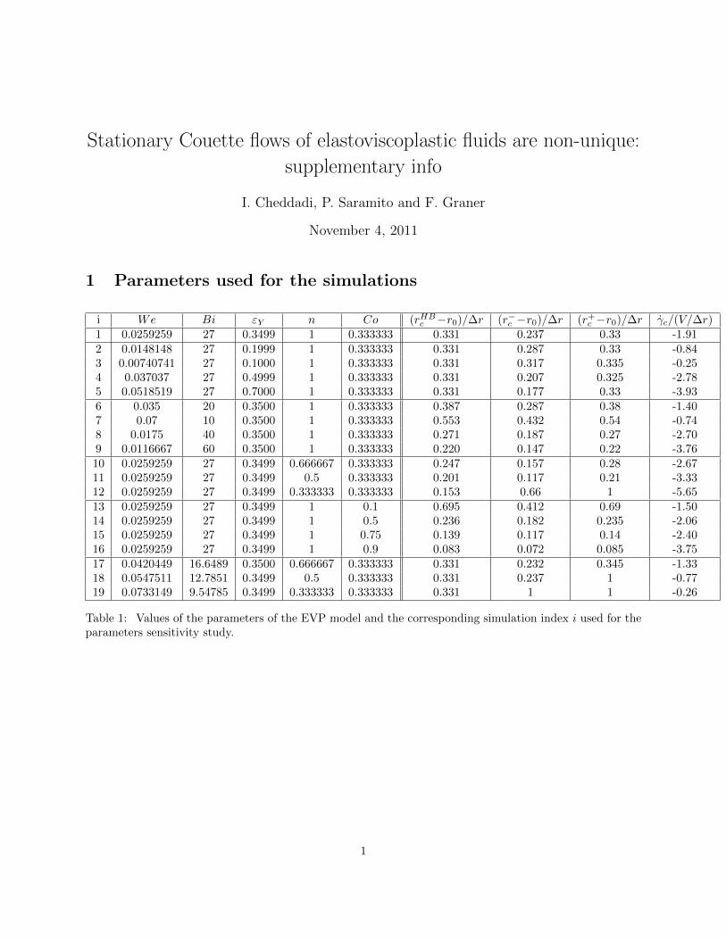
i We Bi εY n Co (rHBc −r0)/∆r (r−c −r0)/∆r (r+c −r0)/∆r γc/(V/∆r)1 0.0259259 27 0.3499 1 0.333333 0.331 0.237 0.33 -1.912 0.0148148 27 0.1999 1 0.333333 0.331 0.287 0.33 -0.843 0.00740741 27 0.1000 1 0.333333 0.331 0.317 0.335 -0.254 0.037037 27 0.4999 1 0.333333 0.331 0.207 0.325 -2.785 0.0518519 27 0.7000 1 0.333333 0.331 0.177 0.33 -3.936 0.035 20 0.3500 1 0.333333 0.387 0.287 0.38 -1.407 0.07 10 0.3500 1 0.333333 0.553 0.432 0.54 -0.748 0.0175 40 0.3500 1 0.333333 0.271 0.187 0.27 -2.709 0.0116667 60 0.3500 1 0.333333 0.220 0.147 0.22 -3.7610 0.0259259 27 0.3499 0.666667 0.333333 0.247 0.157 0.28 -2.6711 0.0259259 27 0.3499 0.5 0.333333 0.201 0.117 0.21 -3.3312 0.0259259 27 0.3499 0.333333 0.333333 0.153 0.66 1 -5.6513 0.0259259 27 0.3499 1 0.1 0.695 0.412 0.69 -1.5014 0.0259259 27 0.3499 1 0.5 0.236 0.182 0.235 -2.0615 0.0259259 27 0.3499 1 0.75 0.139 0.117 0.14 -2.4016 0.0259259 27 0.3499 1 0.9 0.083 0.072 0.085 -3.7517 0.0420449 16.6489 0.3500 0.666667 0.333333 0.331 0.232 0.345 -1.3318 0.0547511 12.7851 0.3499 0.5 0.333333 0.331 0.237 1 -0.7719 0.0733149 9.54785 0.3499 0.333333 0.333333 0.331 1 1 -0.26

Table 1: Values of the parameters of the EVP model and the corresponding simulation index i used for theparameters sensitivity study.

1

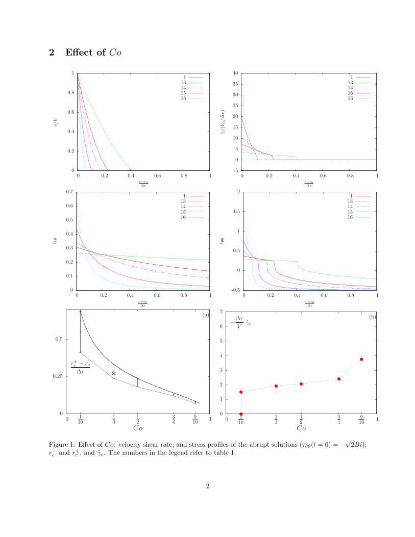
2 Effect of Co

0

0.2

0.4

0.6

0.8

1

0 0.2 0.4 0.6 0.8 1

v/V

r−r0∆r

113141516

-5

0

5

10

15

20

25

30

35

40

0 0.2 0.4 0.6 0.8 1

γ/(V0/∆

r)

r−r0∆r

113141516

0

0.1

0.2

0.3

0.4

0.5

0.6

0.7

0 0.2 0.4 0.6 0.8 1

ε rθ

r−r0∆r

113141516

-0.5

0

0.5

1

1.5

2

0 0.2 0.4 0.6 0.8 1

ε θθ

r−r0∆r

113141516

0

0.25

0.5

0 110

13

12

34

910

1

Co

r±c − r0∆r

(a)

0

1

2

3

4

5

6

7

0 110

13

12

34

910

1

Co

−∆r

Vγc

(b)

Figure 1: Effect of Co: velocity shear rate, and stress profiles of the abrupt solutions (τθθ(t = 0) = −√

2Bi);r−c and r+c , and γc. The numbers in the legend refer to table 1.

2

3 Effect of Bi

0

0.2

0.4

0.6

0.8

1

0 0.2 0.4 0.6 0.8 1

v/V

r−r0∆r

16789

-2

0

2

4

6

8

10

12

14

0 0.2 0.4 0.6 0.8 1

γ/(V0/∆

r)

r−r0∆r

16789

0.1

0.15

0.2

0.25

0.3

0.35

0.4

0 0.2 0.4 0.6 0.8 1

ε rθ

r−r0∆r

16789

-0.5

-0.4

-0.3

-0.2

-0.1

0

0.1

0.2

0.3

0.4

0.5

0.6

0 0.2 0.4 0.6 0.8 1

ε θθ

r−r0∆r

16789

0

0.25

0.5

0 25 50

Bi

r±c − r0∆r

(a)

0

1

2

3

4

5

0 25 50

Bi

−∆r

V0γc

(b)

Figure 2: Effect of Bi: velocity shear rate, and stress profiles of the abrupt solutions (τθθ(t = 0) = −√

2Bi);r−c and r+c , and γc. The numbers in the legend refer to table 1. V0 is the velocity that corresponds to simu1.

3

4 Effect of εY

0

0.2

0.4

0.6

0.8

1

0 0.2 0.4 0.6 0.8 1

v/V

r−r0∆r

12345

-1

0

1

2

3

4

5

6

7

8

9

0 0.2 0.4 0.6 0.8 1

γ/(V0/∆

r)

r−r0∆r

12345

0

0.1

0.2

0.3

0.4

0.5

0.6

0 0.2 0.4 0.6 0.8 1

ε rθ

r−r0∆r

12345

-1

-0.5

0

0.5

1

1.5

0 0.2 0.4 0.6 0.8 1

ε θθ

r−r0∆r

12345

0

0.25

0.5

0 0.5 1

εY

r±c − r0∆r

(a)

0

1

2

3

4

5

0 0.5 1

εY

−∆r

Vγc

(b)

Figure 3: Effect of εY : velocity shear rate, and stress profiles of the abrupt solutions (τθθ(t = 0) = −√

2Bi);r−c and r+c , and γc. The numbers in the legend refer to table 1.

4

4.1 Effect of n

0

0.2

0.4

0.6

0.8

1

0 0.2 0.4 0.6 0.8 1

v/V

r−r0∆r

1101112

-5

0

5

10

15

20

25

30

0 0.2 0.4 0.6 0.8 1

γ/(V0/∆

r)

r−r0∆r

1101112

0.1

0.12

0.14

0.16

0.18

0.2

0.22

0.24

0.26

0.28

0.3

0.32

0 0.2 0.4 0.6 0.8 1

ε rθ

r−r0∆r

1101112

-0.5

-0.4

-0.3

-0.2

-0.1

0

0.1

0.2

0.3

0.4

0 0.2 0.4 0.6 0.8 1

ε θθ

r−r0∆r

1101112

0

0.25

0.5

0 13

12

23

1

n

r±c − r0∆r

(a)

0

1

2

3

4

5

6

7

0 13

12

23

1

n

−∆r

Vγc

(b)

Figure 4: Effect of n: velocity shear rate, and stress profiles of the abrupt solutions (τθθ(t = 0) = −√

2Bi);r−c and r+c , and γc. The numbers in the legend refer to table 1.

5

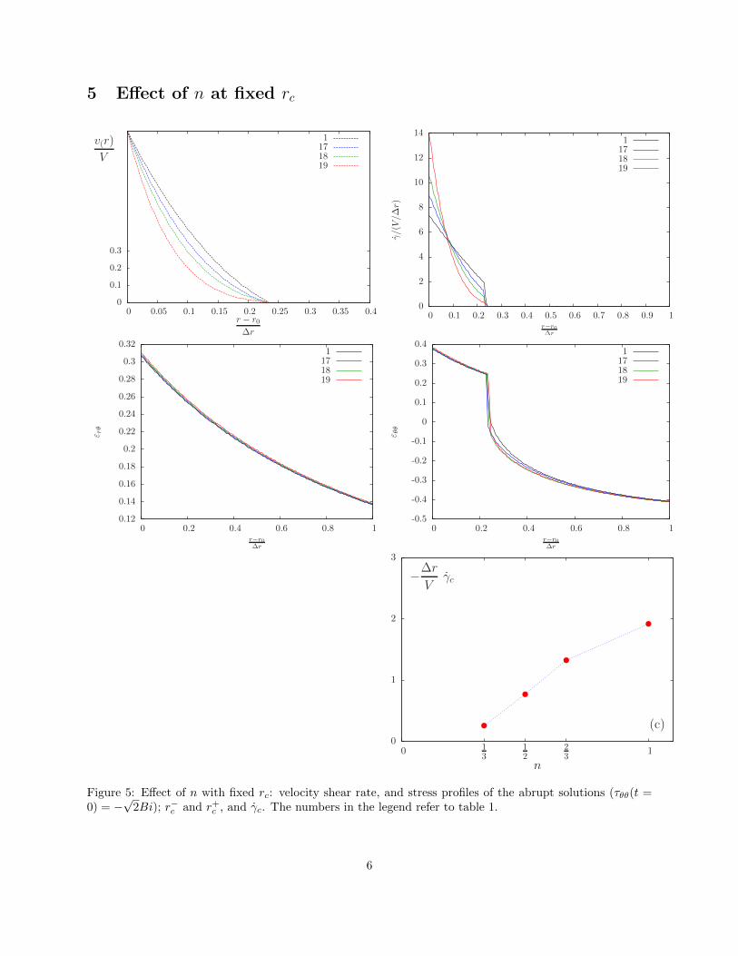
5 Effect of n at fixed rc

0

0.1

0.2

0.3

0 0.05 0.1 0.15 0.2 0.25 0.3 0.35 0.4r − r0∆r

v(r)

V

1171819

0

2

4

6

8

10

12

14

0 0.1 0.2 0.3 0.4 0.5 0.6 0.7 0.8 0.9 1

γ/(V/∆

r)

r−r0∆r

1171819

0.12

0.14

0.16

0.18

0.2

0.22

0.24

0.26

0.28

0.3

0.32

0 0.2 0.4 0.6 0.8 1

ε rθ

r−r0∆r

1171819

-0.5

-0.4

-0.3

-0.2

-0.1

0

0.1

0.2

0.3

0.4

0 0.2 0.4 0.6 0.8 1

ε θθ

r−r0∆r

1171819

0

1

2

3

0 13

12

23

1

n

−∆r

Vγc

(c)

Figure 5: Effect of n with fixed rc: velocity shear rate, and stress profiles of the abrupt solutions (τθθ(t =0) = −

√2Bi); r−c and r+c , and γc. The numbers in the legend refer to table 1.

6