RIGHT:

URL:

CITATION:

AUTHOR(S):

ISSUE DATE:

TITLE:

Evaluation of Earthquake-Induced LocalDamage in Steel Moment-Resisting FramesUsing Wireless Piezoelectric Strain Sensing(Dissertation_全文 )

Li, Xiaohua

Li, Xiaohua. Evaluation of Earthquake-Induced Local Damage in Steel Moment-Resisting Frames Using WirelessPiezoelectric Strain Sensing. 京都大学, 2015, 博士(工学)

2015-09-24

https://doi.org/10.14989/doctor.k19299

許諾条件により本文は2016-09-24に公開

  

Evaluation of Earthquake-Induced Local Damage in

Steel Moment-Resisting Frames Using Wireless

Piezoelectric Strain Sensing

2015

Xiaohua LI

  

 

-i-  

TABLE OF CONTENTS

CHAPTER 1 Introduction

1.1 Background and motivation 1-1

1.2 Objectives 1-3

1.3 Organization 1-3

REFERENCES 1-4

LIST OF PUBLICATIONS 1-8

CHAPTER 2 Scheme of local damage evaluation using wireless piezoelectric

strain sensing

2.1 Overview 2-1

2.2 Influence of local damage on moment distribution 2-1

2.3 Scheme of local damage evaluation 2-5

2.3.1 Concept 2-5

2.3.2 Wireless piezoelectric strain measurement 2-7

2.3.3 Pre-identified damage-prone region and reference point 2-8

2.4 Summary 2-9

REFERENCES 2-9

CHAPTER 3 Strain-based damage index for evaluating seismically induced

beam fracture

3.1 Overview 3-1

3.2 General formulation of damage index 3-1

3.3 Signal processing for extracting damage index 3-4

3.4 Five-story steel frame testbed 3-5

3.4.1 Design of testbed 3-5

3.4.2 Experiment views 3-7

3.5 Preliminary verifications 3-10

3.5.1 Measurement system 3-10

 

-ii-  

3.5.2 Excitations 3-11

3.5.3 Damage patterns 3-12

3.5.4 Damage cases 3-12

3.5.5 Test results 3-13

3.6 Summary 3-18

REFERENCES 3-19

CHAPTER 4 Sensitivity investigation of strain-based damage index

4.1 Overview 4-1

4.2 Numerical studies with a nine-story steel moment-resisting frame 4-1

4.2.1 Nine stories building model 4-1

4.2.2 Analysis model 4-2

4.2.3 Data preprocessing 4-6

4.2.4 Simulation results 4-8

4.3 Sensitivity study using the five-story steel frame testbed 4-11

4.3.1 Excitations for vibration tests 4-12

4.3.2 Sensor location 4-13

4.3.3 Results and discussions 4-15

4.4 Summary 4-20

REFERENCES 4-21

CHAPTER 5 Simplified derivation of a damage curve for seismic beam fracture

5.1 Overview 5-1

5.2 Damage curve 5-1

5.3 Simplified method 5-2

5.3.1 Simplified frame 5-2

5.3.2 Analytical model 5-4

5.3.3 Parametric analysis 5-7

5.3.4 Simplified closed-form expression 5-11

5.4 Verifications 5-14

5.4.1 SAC nine-story steel moment-resisting frame 5-14

5.4.2 Five-story steel frame testbed 5-20

5.5 Summary 5-23

 

-iii-  

REFERENCES 5-24

CHAPTER 6 Decoupling interaction between multiple beam fractures

6.1 Overview 6-1

6.2 Influence of moment release 6-1

6.3 Decoupling method 6-3

6.4 Numerical studies 6-4

6.5 Experimental investigations 6-10

6.6 Summary 6-14

REFERENCES 6-15

CHAPTER 7 Conclusions and future studies

7.1 Conclusions 7-1

7.2 Future studies 7-3

REFERENCES 7-5

 

Acknowledgments

 

-iv-  

 

1-1  

CHAPTER 1

Introduction

1.1 Background and motivation

Steel moment-resisting frame buildings have been widely adopted in earthquake-prone areas

since the early 1970s, due to their excellent features such as ease construction, architectural and

functional versatility, and high plastic deformation capacity. The seismic design of these buildings

allowed that structural elements deform in-elastically in large earthquakes, which is useful for

dissipating energy. Nevertheless, welds and/or bolts at beam-to-column connections are not

sufficiently ductile for high stress states. After a great earthquake, these buildings excited by severe

ground shaking may suffer brittle fractures and/or bolt slippage at beam-to-column connections,

which possibly classify them to be unsafe for occupancy. As witnessed in the 1994 Northridge

earthquake and 1995 Kobe earthquake, a large number of steel moment-resisting frames suffered

brittle fractures at steel beam-to-column connections [1-3]. The most commonly observed fracture

damage initiated at the weld toe on bottom flange near the weld access hole. In some cases, severe

brittle fractures extended to the web and the whole moment resisting connections failed.

Post-quake safety evaluation and decision-making on re-occupancy for the earthquake-affected

steel buildings depends on the results of the inspection of damage to beam-to-column connections

in frames. Conventionally, non-destructive evaluation (NDE) techniques such as visual examination

and ultrasonic testing were used to detect seismic local damage. Nonetheless, these methods require

extensive costs and labors because steel members are covered with fire-proofing and architectural

finishes. Moreover, in the surveys of steel moment-resisting frames affected by the 1994 Northridge

earthquake and 1995 Kobe earthquake, while many damaged connections were discovered,

numerous connections that remained intact had to be inspected because of obvious damage in

concrete slabs or nonstructural elements around these connections.

 

1-2  

Structural health monitoring (SHM), which enables structural engineers or owners to evaluate

damage in structures in a prompt and objective manner, is acknowledged as one of promising tools

to support rapid damage assessment and decision-making following earthquakes [4]. At present, a

few important steel buildings located at metropolitan areas with high seismicity have installed SHM

systems as an extension of strong ground motion monitoring systems, where the floor responses

(e.g., acceleration and velocity) are primarily measured [5-9]. For SHM applications, damage

identification methods, such as modal parameter-based method [10], inter-story drift ratio-based

method [11], seismic wave propagation method [12], and time series analysis method [13], which

utilize the global characteristics of buildings (e.g., acceleration responses, modal frequency and

mode shape, and inter-story drift ratio) have been extensively studied over the past few decades.

Experimental investigations into these methods demonstrated that they estimated the health

conditions of buildings to some extent, but encountered serious challenges to give reliable

information of localized damage on structural members. For example, through a series of shaking

table testing in which various levels of realistic seismic damage were reproduced for a high-rise

steel building specimen at the E-Defense facility in Japan, Ji et al. [14] demonstrated that the

natural frequencies of the specimen decreased by 4.1%, 5.4%, and 11.9% on average for three

damage levels respectively, while the mode shapes changed very little. The changes in the modal

properties were largely influenced by cracks in concrete slabs and barely provided the accurate

location and extent of seismic damage on individual steel members. Besides, through the same

testing, Chung [15] reported large variations in seismic damage at beam-column connections at the

same floor level that experienced nearly identical deformation due to large uncertainties in materials

and hysteresis behaviors of members and connections.

With the development of microprocessor and wireless communication technologies and

declining in cost, wireless sensing as an alternative to wire monitoring has the potential to

fundamentally change health monitoring technology [16-18]. Wireless sensing is a spatially

distributed autonomous sensor network. Its features are wireless communication, on-board

computation, small size and low cost. Wireless sensing allows largely increasing the density of

sensors installed in large-scale civil structures with reasonable investments. Moreover, as strain

responses directly reflect the local damage information of the monitored structural members [19-22],

piezoelectric strain sensors (e.g., lead zirocondate titanate (PZT) and polyvinylidene fluoride

(PVDF)) which have high sensitivity, wide frequency range, and long-term durability, open up

another new opportunity to improve conventional health monitoring [23-26]. Thus, by combining

wireless sensing with piezoelectric strain sensors, one can form dense-array wireless strain sensing

systems for localized damage detection in steel moment-resisting frame buildings.

 

1-3  

1.2 Objectives

The target of this dissertation is to develop a localized damage evaluation method specifically

designed for detecting and quantifying seismically induced fractures to beam-to-column

connections in steel moment-resisting frame buildings, which enables to rapidly and reliably

estimate the remaining capacity of the earthquake-affected buildings and thus support post-quake

decision-making on re-occupancy. In this dissertation, the following topics are studied.

(1) A high-sensitivity wireless strain sensing system is developed to measure strain responses

under small-amplitude dynamic loads (e.g., ambient vibration and minor earthquake ground

shaking).

(2) A strain-based damage index is presented from a comparative study of strain responses

measured on steel beams at the intact conditions and after major earthquakes for evaluating

seismically induced beam fractures.

(3) The sensitivity of the strain-based damage index to measurement environments and various

structural parameters is investigated. It includes the independency of the damage index on input

excitations and vibrational modes, the influence of sensor location on the damage index, the effect

of interaction between multiple damages on the damage index, and the general applicability of the

damage index.

(4) A closed-form expression of damage curve for single damage condition is derived to quantify

the damage extent of beam fractures. The damage curve expresses the damage index as a function

of reduction in bending stiffness of the fractured section.

(5) A decoupling method of estimating the damage index for multiple damages is presented for

damage quantification of multiple beam fractures using the presented damage curve.

1.3 Organization

The dissertation comprises seven chapters. Chapter 1 introduces the background and motivation,

and aims of the research. Chapters 2 to 6 contain the main contents of the thesis: (1) scheme of

localized damage evaluation with wireless piezoelectric stain sensing; (2) general formulation of

strain-based damage index; (3) sensitivity study of the damage index; (4) derivation of damage

curve for single damage condition; (5) decoupling method of estimating damage index for multiple

damages. Chapter 7 summarizes the main findings of the dissertation.

Chapter 2 introduces the conceptual scheme of localized damage evaluation using wireless

piezoelectric strain sensing. Local damage such as brittle fracture at beam ends changes the

 

1-4  

distribution of bending moments in steel moment-resisting frames. When frames behave linearly,

the bending moments can be estimated by measuring strain responses. Thus, local damage can be

identified from strain information. In the scheme, a wireless strain sensing system formed of a

wireless sensor network and polyvinylidene fluoride strain sensors is designed to monitor strain

responses. Moreover, the pre-identification of damage-prone region in steel frames using demand

prediction methods is discussed.

Chapter 3 presents a strain-based damage index that is capable of evaluating seismically induced

beam fractures in steel moment-resisting frames. The damage index is formulated from a

comparative study of dynamic strain responses of steel beams monitored under ambient vibration

before and after earthquakes. Then, a step-by-step signal processing procedure for extracting the

damage index is presented. Finally, the effectiveness of the damage index and the associated

wireless strain sensing system are examined with a series of vibration tests using a five-story steel

frame testbed.

Chapter 4 further investigates the sensitivity of the presented damage index to measurement

environments and various structural parameters. The sensitivity of the damage index is examined

through numerical studies with a nine-story steel moment-resisting frame and experimental studies

using the five-story steel frame testbed.

Chapter 5 presents a closed-form expression of damage curve where strain-based damage index

is a function of reduction in beam bending stiffness induced by fracture. The damage curve allows

quantitative evaluation on earthquake-induced fractures on beams. In addition, this chapter

demonstrates that the presented damage curve is generally applicable for common multi-story

multi-bay steel moment-resisting frames. The effectiveness of the damage curve is verified

numerically using a nine-story steel moment-resisting frame model and experimentally using the

one-quarter-scale five-story steel frame testbed.

Chapter 6 presents a decoupling method of estimating damage index for multiple beam fractures

in order to quantify their damage extents using the damage curve presented in Chapter 5. Firstly, the

mechanism of moment release and influence is demonstrated with a simple sub-frame. Then, the

framework and algorithm of the decoupling method is presented. Finally, the effectiveness of the

decoupling method is verified numerically through a nine-story steel moment-resisting frame and

experimentally using the five-story steel frame testbed.

REFERENCES

[1] Nakashima M. (1995). Reconnaissance report on damage to steel buildings structures

 

1-5  

observed from the 1995 Hyogoken-Nanbu (Hanshin/Awaji) earthquake, Abridged English

edition. Steel Committee of Kinki Branch, the Architectural Institute of Japan (AIJ).

[2] Mahin S. (1998). Lessons from damage to steel buildings during the Northridge earthquake.

Engineering Structures, 20(4-6): 261-270.

[3] Youssef N., Bonowitz D., and Gross J. (1995). A survey of steel moment-resisting frame

buildings affected by the 1994 northridge earthquake. NISTIR 5625.

[4] Celebi M., Sanli A., Sinclair M., Gallant S., and Radulescu D. (2004). Real-time seismic

monitoring needs of a building owner - and the solution: a cooperative effort. Earthquake

Spectra, 20(2): 333-346.

[5] Kalkan E., Banga K., Ulusoy H. S., Fletcher J. P. B., Leith W. S., Reza S., and Cheng T.

(2012). Advanced earthquake monitoring system for U.S. Department of Veterans Affairs

medical buildings—instrumentation. U.S. Geological Survey Open-File Report 2012–1241,

143 p.

[6] Naeim F., Hagie H., Alimoradi A., and Miranda E. (2005). Automated post-earthquake

damage assessment and safety evaluation of instrumented buildings. A Report to CSMIP

(JAMA Report No. 2005–10639), John A. Martin & Associates.

[7] Rahmani M., and Todorovska M. (2015). Structural health monitoring of a 54-story steel-

frame building using a wave method and earthquake records. Earthquake Spectra, 31(1): 501-

525.

[8] Rodgers J., and Celebi M. (2006). Seismic response and damage detection analyses of an

instrumented steel moment-framed building. Journal of Structural Engineering, 132(10):

1543-1552.

[9] Siringoringo D., and Fujino Y. (2015). Seismic response analyses of an asymmetric base-

isolated building during the 2011 Great East Japan (Tohoku) Earthquake. Structural control

and health monitoring, 22: 71-90.

[10] Fan W., Qiao P. (2011). Vibration-based damage identification methods: a review and

comparative study. Structural health monitoring, 10(1): 83-111.

[11] Naeim, F., Lee, H., Hagie, H., Bhatia, H., Alimoradi, A., and Miranda, E. (2006). Three-

dimensional analysis, real-time visualization, and automated post-earthquake damage

assessment of buildings. Struct. Design Tall Spec. Build., 15: 105-138.

[12] Todorovska M., Trifunac M. (2008). Impulse response analysis of the Van Nuys 7-storey hotel

during 11 earthquakes and earthquake damage detection. Structural Control and Health

Monitoring, 15(1): 90-116.

[13] Sohn H., Farrar C. (2001). Damage diagnosis using time series analysis of vibration signals.

 

1-6  

Smart Materials and Structures, 10(3): 446-451.

[14] Ji X, Fenves G, Kajiwara K, and Nakashima M. (2011). Seismic damage detection of a full-

scale shaking table test structure. Journal of Structural Engineering, 137(6): 14-21. DOI:

10.1061/(ASCE)ST.1943-541X.0000278.

[15] Chung Y. (2010). Existing performance and effect of retrofit of high-rise steel buildings

subjected to long-period ground motions. Doctoral Dissertation, Kyoto University, Japan,

September, 2010.

[16] Lynch P. J. (2005). Design of a wireless active sensing unit for localized structural health

monitoring. Struct. Control Health Monit., 12: 405-423.

[17] Spencer Jr B. F., Ruiz-Sandoval M. E., and Kurata N. (2004). Smart sensing technology:

opportunities and challenges. Struct. Control Health Monit., 11: 349-368.

[18] Park J., Sim S., and Jung H. (2013). Wireless sensor network for decentralized damage

detection of building structures. Smart Structures and Systems, 12(3-4): 399-414.

[19] Li S., Wu Z. (2007). Development of distributed long-gage fiber optic sensing system for

structural health monitoring. Structural health monitoring, 6(2): 133-143.

[20] Hong W., Wu Z., Yang C., Wan C., and Wu G. (2012). Investigation on the damage

identification of bridges using distributed long-gauge dynamic macrostrain response under

ambient excitation. Journal of Intelligent Material Systems and Structures, 23(1): 85-103.

[21] Razi P., Esmaeel R., and Taheri F. (2013). Improvement of a vibration-based damage

detection approach for health monitoring of bolted flange joints in pipelines. Structural health

monitoring, 12(3): 207-224.

[22] Mujica L., Vehi J., Staszewski W., and Worden K. (2008). Impact damage detection in aircraft

composites using knowledge-based reasoning. Structural health monitoring, 7(3): 215-230.

[23] Park G., and Inman D. (2007). Structural health monitoring using piezoelectric impedance

measurements. Philosophical Transactions of the Royal Society A, 365: 373-392.

[24] Cuc A., Giurgiutiu V., Joshi S., and Tidwell Z. (2007). Structural health monitoring with

piezoelectric wafer active sensors for space applications. AIAA Journal, 45(12): 2838-2850.

[25] Najib A., Emmanuel M., Jamal A., Farouk B., Sébastien G., and Youssef Z. (2011).

Application of Piezoelectric Transducers in Structural Health Monitoring Techniques.

Advances in Piezoelectric Transducers, Dr. Farzad Ebrahimi (Ed.), ISBN: 978-953-307-931-

8, InTech, Available from: http://www.intechopen.com/books/advances-in-piezoelectric-

transducers/application-of-piezoelectrictransducers-in-structural-health-monitoring-

techniques

[26] Giurgiutiu V., Zagrai A., and Bao J. (2002). Piezoelectric wafer embedded active sensors for

 

1-7  

aging aircraft structural health monitoring. Structural Health Monitoring, 1(1): 41-61.

 

1-8  

LIST OF PUBLICATIONS

Journal papers

[1] Li X., Kurata M., and Nakashima M. (2015). “Simplified derivation of a damage curve for

seismically induced beam fracture in steel moment-resisting frames.” Journal of Structural

Engineering (ASCE). (under review)

[2] Li X., Kurata M., and Nakashima M. (2015). “Evaluating damage extent of fractured beams

in steel moment-resisting frames using dynamic strain responses.” Earthquake Engineering &

Structural Dynamics, 44, 563-581. DOI: 10.1002/eqe.2536.

[3] Kurata M., Li X., Fujita K., and Yamaguchi M. (2013). “Piezoelectric dynamic strain

monitoring for detecting local seismic damage in steel buildings.” Smart Materials and

Structures, 22, 115002. DOI:10.1088/0964-1726/22/11/115002.

[4] Li X., Kurata M., Fujita K., Yamaguchi M., and Nakashima M. (2013). “Detection of Local

Damage in Steel Moment-Resisting Frames Using Wireless PVDF Sensing,” Journal of

Constructional Steel, Japanese Society of Steel Construction, 21, 259-264.

[5] Li X., Gong M., and Xie L. (2011). “Structural physical parameter identification using

Bayesian estimation based on multi-resolution analysis: formulation and verification.”

Engineering Mechanics, 28(1):12-18. (in Chinese)

[6] Li X., Xie L., and Gong M. (2010). “Structural physical parameter identification using

Bayesian estimation with Markov Chain Monte Carlo methods.” Journal of Vibration and

Shock, 29(4):59-63. (in Chinese)

International conference papers

[1] Li X., Kurata M., and Nakashima M. (2013). “Dynamic strain monitoring for detecting

fracture damage at beam-ends in steel moment-resisting frames.” Proceedings of the 6th

International Conference on Structural Health Monitoring of Intelligent Infrastructure, Hong

Kong, China.

[2] Kurata M., Li X., Fujita K., He L., and Yamaguchi M. (2013). “PVDF piezo film as dynamic

strain sensor for local damage detection of steel frame buildings.” Proc. SPIE 8692, Sensors

and Smart Structures Technologies for Civil, Mechanical, and Aerospace Systems 2013,

86920F. doi:10.1117/12.2009554.

[3] Kurata M., Fujita K., Li X., Yamazaki T., and Yamaguchi M. (2013). “Development of cyber-

based autonomous structural integrity assessment system for building structures.” Proc. SPIE

 

1-9  

8692, Sensors and Smart Structures Technologies for Civil, Mechanical, and Aerospace

Systems 2013, 86924E. doi:10.1117/12.2009589.

[4] Suzuki A., Kurata M., Li X., Minegishi K., Tang Z., and Burton A. (2015). “Quantification of

seismic damage in steel beam-column connection using PVDF strain sensors and model-

updating technique.” Proc. SPIE 9435, Sensors and Smart Structures Technologies for Civil,

Mechanical, and Aerospace Systems 2015, 94352E. doi:10.1117/12.2085300.

Domestic conference papers

[1] Li X., Kurata M., and Nakashima M. (2012). “Story stiffness identification of full-scale test

structure using Bayesian model updating method.” Summaries of Technical Papers of Annual

Meeting Kinki branch, AIJ, No.52, pp.85-88.

[2] Li X., Kurata M., and Nakashima M. (2012). “Story stiffness identification of full-scale test

structure using Bayesian model updating method.” Summaries of technical papers of annual

meeting 2012 (構造 II), AIJ, pp.589-590.

[3] Kurata M., Li X., Fujita K., Yamaguchi M., He L., and Nakashima M. (2013). “Detection of

beam-end fracture by monitoring dynamic strain in steel structures: Part 1. Concept and

testbed design.” Summaries of technical papers of annual meeting 2013 (構造 II), AIJ, pp.89-

90.

[4] Li X., Kurata M., Fujita K., Yamaguchi M., and Nakashima M. (2013). “Detection of beam-

end fracture by monitoring dynamic strain in steel structures: Part 2. Vibration testing.”

Summaries of technical papers of annual meeting 2013 (構造 II), AIJ, pp.91-92.

[5] Yamazaki T., Fujita K., Kurata M., and Li X. (2013). “Cyber-aided dense array monitoring for

autonomous visualization of local damage extent in steel buildings: Part 1. Design of cyber

platform.” Summaries of technical papers of annual meeting 2013 (構造 II), AIJ, pp.101-102.

[6] Fujita K., Kurata M., Li X., and Yamazaki T. (2013). “Cyber-aided dense array monitoring for

autonomous visualization of local damage extent in steel buildings: Part 2. Benchmark

testing.” Summaries of technical papers of annual meeting 2013 (構造 II), AIJ, pp.103-104.

[7] Kurata M., Li X., Fujita K., Yamaguchi M., and He L. (2013). “Strain-based monitoring of

local damage in steel structures: Part I Concept and testbed design.” Summaries of Technical

Papers of Annual Meeting Kinki branch, AIJ, No.53, pp.169-172.

[8] Li X., Kurata M., Fujita K., and Yamaguchi M. (2013). “Dynamic strain monitoring for local

damage detection in steel structures: Part 2. Experimental results.” Summaries of Technical

Papers of Annual Meeting Kinki branch, AIJ, No.53, pp.173-176.

 

1-10  

[9] Li X., Kurata M., and Nakashima M. (2014). “Sensitivity study of dynamic strain-based

damage index for evaluating beam damage in steel buildings.” Summaries of Technical

Papers of Annual Meeting Kinki branch, AIJ, No.54, pp.177-180.

[10] Li X., Kurata M., and Nakashima M. (2014). “Damage quantification of beam seismic

fracture in steel buildings.” Summaries of technical papers of annual meeting 2014 (構造 II),

AIJ, pp.109-110.

 

2-1  

CHAPTER 2

Scheme of local damage evaluation using wireless piezoelectric strain

sensing

2.1 Overview

In steel moment-resisting frames, local damage such as seismically-induced fractures on steel

beams changes the distribution of bending moments sustained by members. The moment

distribution is independent of external loadings when it is evaluated at a natural vibrational mode. In

practice, for the frames behaving linearly, the bending moments can be estimated by measuring

strain responses in the members. Thus, local damage can be evaluated by monitoring strain

responses. This chapter introduces a scheme of seismically-induced local damage evaluation using

wireless piezoelectric strain sensing. Firstly, the influence of local damage on moment distributions

in steel frames is illustrated using a simple frame. Then, the scheme of local damage evaluation is

presented.

2.2 Influence of local damage on moment distribution

Inclusion of local damage on steel beams reduces the bending moments resisted by the damaged

beams, which attributes mainly to the decreases of the bending stiffness of the beams. The

following analytical study for a simple frame demonstrates a quantitative relationship between the

reduction in the modal bending moment and a beam fracture.

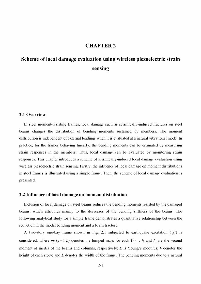
A two-story one-bay frame shown in Fig. 2.1 subjected to earthquake excitation )(tu g is

considered, where mi ( 2,1i ) denotes the lumped mass for each floor; Ib and Ic are the second

moment of inertia of the beams and columns, respectively; E is Young’s modulus; h denotes the

height of each story; and L denotes the width of the frame. The bending moments due to a natural

 

2-2  

mode are obtained using the equivalent static forces method [1]. At any instant of time t, the

equivalent static forces fs(t) = [f1(t), f2(t)] associated with a natural mode are the external forces that

act on the frame as illustrated in Fig. 2.1.

Fig. 2.1 Two-story frame model

To simplify the formulation, we note that

( 1)L a h a , (2.1a)

)10( kIkI cb . (2.1b)

where a denotes the aspect ratio of the frame and k denotes the stiffness ratio between the beams

and columns. Assuming that the frame behaves linearly under small amplitude excitations, the

bending moments at points A and B at any instant of time t are calculated by the force method of

structural analysis as

1 1 2 2( ) ( ) ( )AM t A f t A f t , (2.2a)

3 1 4 2( ) ( ) ( )BM t A f t A f t . (2.2b)

where A1, A2, A3, and A4 are:

1 2 2

6

180 90 5

ahkA

k ak a

, (2.3a)

0.1L

0.1L

L

h

h

EIb

EIc

EIc

m2

m1

EIc

EIc

A

B

)(tug

Damaged part:

)(2 tf

)(1 tf

)10( bEI

 

2-3  

2

2 2 2

36 24

180 90 5

hk ahkA

k ak a

, (2.3b)

2

3 2 2

36 6

180 90 5

hk ahkA

k ak a

, (2.3c)

2

4 2 2

72 18

180 90 5

hk ahkA

k ak a

. (2.3d)

In modal analysis, the equivalent static forces fs(t) associated with a natural mode (e.g., the ith

mode, i = 1, 2) can be expressed as

2( ) ( )is i it q t mΦf , or 1 12 1

2 2 2

( )( )

( )

ii

i i

f t mq t

f t m

(2.4)

where i and iΦ are the ith modal frequency and mode shape, respectively, and )(tqi is the modal

coordinate for the ith mode. Equation (2.4) indicates that the relationship between equivalent static

forces corresponding to the first and second floor masses is constant for a linear vibrating system

where the mode shape is invariant:

2 1( ) ( )if t u f t (2.5)

where 2 2 1 1/i i iu m m .

The bending moments at points A and B due to the ith mode at any instant of time t are

expressed as follows.

22

1 121

(24 36 )

80 90( ) ( )

5

6ii i

A ik ak a

a k hku ahkM t m q t

, (2.6a)

22

1 12

6 (3 12 ) 6 (

180

6 )( ) )

9 5(

0

ii i

B ik

hk a k u hk a kM t

ak at m q

. (2.6b)

 

2-4  

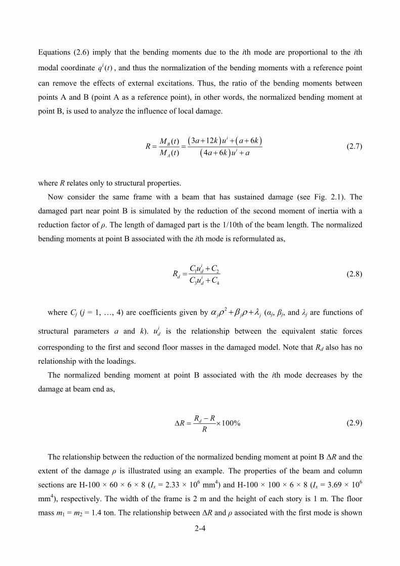
Equations (2.6) imply that the bending moments due to the ith mode are proportional to the ith

modal coordinate )(tqi , and thus the normalization of the bending moments with a reference point

can remove the effects of external excitations. Thus, the ratio of the bending moments between

points A and B (point A as a reference point), in other words, the normalized bending moment at

point B, is used to analyze the influence of local damage.

3 12 6( )

( ) 4 6

iB

iA

a k u a kM tR

M t a k u a

(2.7)

where R relates only to structural properties.

Now consider the same frame with a beam that has sustained damage (see Fig. 2.1). The

damaged part near point B is simulated by the reduction of the second moment of inertia with a

reduction factor of ρ. The length of damaged part is the 1/10th of the beam length. The normalized

bending moments at point B associated with the ith mode is reformulated as,

1 2

3 4

id

d id

C u CR

C u C

(2.8)

where Cj (j = 1, …, 4) are coefficients given by 2j j j (αj, βj, and λj are functions of

structural parameters a and k). idu is the relationship between the equivalent static forces

corresponding to the first and second floor masses in the damaged model. Note that Rd also has no

relationship with the loadings.

The normalized bending moment at point B associated with the ith mode decreases by the

damage at beam end as,

100%dR RR

R

(2.9)

The relationship between the reduction of the normalized bending moment at point B ΔR and the

extent of the damage ρ is illustrated using an example.  The properties of the beam and column

sections are H-100 × 60 × 6 × 8 (Ix = 2.33 × 106 mm4) and H-100 × 100 × 6 × 8 (Ix = 3.69 × 106

mm4), respectively. The width of the frame is 2 m and the height of each story is 1 m. The floor

mass m1 = m2 = 1.4 ton. The relationship between ΔR and ρ associated with the first mode is shown

 

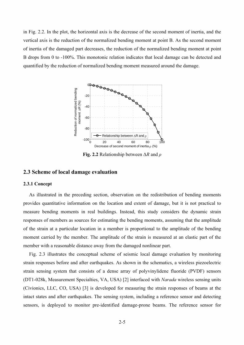
2-5  

in Fig. 2.2. In the plot, the horizontal axis is the decrease of the second moment of inertia, and the

vertical axis is the reduction of the normalized bending moment at point B. As the second moment

of inertia of the damaged part decreases, the reduction of the normalized bending moment at point

B drops from 0 to -100%. This monotonic relation indicates that local damage can be detected and

quantified by the reduction of normalized bending moment measured around the damage.

Fig. 2.2 Relationship between ΔR and ρ

2.3 Scheme of local damage evaluation

2.3.1 Concept

As illustrated in the preceding section, observation on the redistribution of bending moments

provides quantitative information on the location and extent of damage, but it is not practical to

measure bending moments in real buildings. Instead, this study considers the dynamic strain

responses of members as sources for estimating the bending moments, assuming that the amplitude

of the strain at a particular location in a member is proportional to the amplitude of the bending

moment carried by the member. The amplitude of the strain is measured at an elastic part of the

member with a reasonable distance away from the damaged nonlinear part.

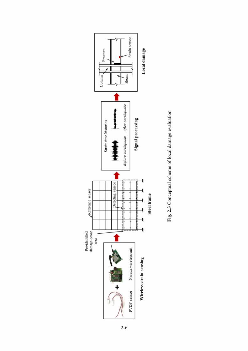
Fig. 2.3 illustrates the conceptual scheme of seismic local damage evaluation by monitoring

strain responses before and after earthquakes. As shown in the schematics, a wireless piezoelectric

strain sensing system that consists of a dense array of polyvinylidene fluoride (PVDF) sensors

(DT1-028k, Measurement Specialties, VA, USA) [2] interfaced with Narada wireless sensing units

(Civionics, LLC, CO, USA) [3] is developed for measuring the strain responses of beams at the

intact states and after earthquakes. The sensing system, including a reference sensor and detecting

sensors, is deployed to monitor pre-identified damage-prone beams. The reference sensor for

0 20 40 60 80 100-100

-80

-60

-40

-20

0

Decrease of second moment of inertia (%)

Re

du

ctio

n o

f no

rma

lize

d b

en

din

g

mo

me

nt

R (

%)

Relationship between R and

 

2-6  

Fig

. 2.3

Con

cept

ual s

chem

e of

loca

l dam

age

eval

uati

on

 

2-7  

normalization is used to eliminate the effects of the excitations. The detecting sensor near probable

damage is used to detect and quantify the local damage. The re-distribution of the bending moment

associated with a natural mode is estimated from the dynamic strain response using signal

processing techniques.

2.3.2 Wireless piezoelectric strain measurement

With the emergence of wireless sensing and piezoelectric materials technologies, one can form

dense-array wireless strain sensing systems for large-scale civil structures with reasonable

investments. Thus, this study develop a wireless piezoelectric strain measurement system

particularly designed for monitoring steel moment-resisting frames using PVDF sensors and

customized wireless sensing units.

The PVDF sensor comprises of a flexible film with silver ink screen printed electrodes covered

by insulating urethane coating. While conventional foil strain gauges are resistive sensors and

require a switch box to convert strain into voltage, the PVDF sensors generate electric charge and

produce voltage in proportion to compressive or tensile mechanical stress or strain, making it an

ideal dynamic strain gauge. The biggest advantage of the PVDF film is its high sensitivity about 60

dB higher than the voltage output of a foil strain gage. This enables the PVDF sensor to measure the

strain time history in steel beams under small dynamic loadings such as ambient vibrations. By

removing a static load from a fixed-supported single beam, the calibration factor of PVDF sensor

attached to a steel beam was estimated approximately as 12mV per micro strain. The other notable

advantages of the PVDF sensor include 1) flexibility for easy deployment, 2) a broad-band

operating frequency throughout the high audio (>1 kHz) and ultrasonic (up to 100 MHz) range, 3)

long term durability with an operating temperature range of −40 to +60°C.

Due to these advantages, PVDF films have been utilized in applications of local damage

detection of civil and mechanical structures in recent decades [4-8]. Wang et al. (1999) proposed an

in-situ method for monitoring the tension of stayed cables of cable-stayed bridges through

embedding PVDF sensors into the cables [4]. Yu et al. (2011) presented a wireless measurement

system with PVDF sensors for monitoring the structural impact responses and the detection of

damage in a bridge model [7].

An emerging wireless technology has great potential for reducing the cost and effort associated

with the installation of the sensing system. The Narada wireless unit is designed with an on-board

analog-to-digital converter (ADC) supporting high-speed data collection (up to 100 kHz) on four

sensor channels [3]. The resolution of the ADC is 16-bits which is often considered a minimum

 

2-8  

resolution for ambient response monitoring. The Narada communicates on the 2.4 GHz IEEE

802.15.4 radio standard (IEEE 2006) using a Texas Instruments CC2420 transceiver. The output

power of the CC2420 transceiver can be varied from 0 to −25 dB with the highest power setting (0

dB) achieving a line-of-sight communication range of approximately 100 m when a 2.2 dBi swivel

antenna (Titanis 2.4 GHz Swivel SMA Antenna) is equipped. The communication range can be

further extended with the use of a high gain antenna.

2.3.3 Pre-identified damage-prone region and reference point

Steel moment-resisting frames have been popular in many regions of high seismicity. Most

codes and design guidelines adopt the strong-column and weak-beam philosophy in design of steel

moment-resisting frames. This design philosophy enhances overall seismic resistance and prevents

development of a soft-story mechanism in a multistory frame. Thus, properly designed steel frames

are prone to suffer seismic damage at beams rather than at columns. This allows the local damage

evaluation system deployed only to beams.

Seismic damage to beam-to-column connections in the steel moment-resisting frames relates to

story deformation demands, i.e., maximum inter-story drift. Thus, damage-prone beams can be pre-

identified using the demand prediction methods, such as inelastic time history analysis and

pushover analysis. This will greatly reduce the density of the wireless strain sensing system. Several

floors likely sustaining large deformation are particularly monitored.

Reference point needs to be located in the undamaged floor for evaluating damage on beams. A

floor with small deformation (e.g., the roof) is recommended for the reference point where the

concrete slabs and beams at the floor remain undamaged. A twenty-story steel moment-resisting

frame was studies to illustrate the procedure to identify damage-prone floors and to select

undamaged floors for a reference point. The twenty-story steel moment-resisting frame designed

according to the pre-Northridge design practice in Los Angeles, California was used. This frame

was intensively studied in the SAC steel project and whose details were in FEMA-355C [9].

Inelastic time history analyses were conducted to predict the maximum story drifts under

earthquake ground motions. The analysis was conducted using the finite element analysis software,

SAP2000. The frame subjected to the 2/50 set of SAC Los Angeles ground motion records was

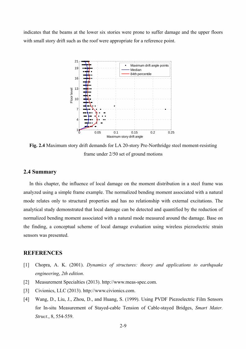
studied [9]. Fig. 2.4 illustrates the maximum story drifts under twenty ground motions, and the

median and 84th percentile values. The maximum story drifts had a very large dispersion in the

lower six stories, and a smaller dispersion in the upper stories. The median and 84th percentile

values of the maximum story drifts were larger at the lower six stories than at the upper stories. This

 

2-9  

indicates that the beams at the lower six stories were prone to suffer damage and the upper floors

with small story drift such as the roof were appropriate for a reference point.

Fig. 2.4 Maximum story drift demands for LA 20-story Pre-Northridge steel moment-resisting

frame under 2/50 set of ground motions

2.4 Summary

In this chapter, the influence of local damage on the moment distribution in a steel frame was

analyzed using a simple frame example. The normalized bending moment associated with a natural

mode relates only to structural properties and has no relationship with external excitations. The

analytical study demonstrated that local damage can be detected and quantified by the reduction of

normalized bending moment associated with a natural mode measured around the damage. Base on

the finding, a conceptual scheme of local damage evaluation using wireless piezoelectric strain

sensors was presented.

REFERENCES

[1] Chopra, A. K. (2001). Dynamics of structures: theory and applications to earthquake

engineering, 2th edition.

[2] Measurement Specialties (2013). http://www.meas-spec.com.

[3] Civionics, LLC (2013). http://www.civionics.com.

[4] Wang, D., Liu, J., Zhou, D., and Huang, S. (1999). Using PVDF Piezoelectric Film Sensors

for In-situ Measurement of Stayed-cable Tension of Cable-stayed Bridges, Smart Mater.

Struct., 8, 554-559.

0 0.05 0.1 0.15 0.2 0.251

4

7

10

13

16

19

21

Maximum story drift angle

Flo

or

leve

l

Maximum drift angle pointsMedian84th percentile

 

2-10  

[5] Liao, W., Wang, D., and Huang, S. (2001). Wireless monitoring of cable tension of cable-

stayed bridge using PVDF piezoelectric films, Journal of Intelligent Material Systems and

Structures, 12, 331-339.

[6] Sumali, H., Meissner, K., and Cudney, H. (2001). A piezoelectric array for sensing vibration

modal coordinates,” Sensors and Actuators A, 93, 123-131.

[7] Yu, Y., Zhao, X., Wang, Y., and Ou, J. (2011). A study on PVDF sensor using wireless

experimental system for bridge structural local monitoring, Telecommunication System, 1-10.

[8] Huha, Y-H., Kim, J., Lee, J., Hong, S., and Park, J. (2011). Application of PVDF film sensor

to detect early damage in wind turbine blade components, Procedia Engineering, 10, 3304-

3309.

[9] FEMA-355C (2000). State of the art report on systems performance of steel moment frames

subject to earthquake ground shaking.

 

3-1  

CHAPTER 3

Strain-based damage index for evaluating seismically induced beam

fracture

3.1 Overview

The primary objective of this chapter is to present and formulate a damage index from strain

responses that is capable of evaluating seismically induced beam fractures in steel moment-resisting

frames. In this chapter, first a novel damage index based on the monitoring of dynamic strain

responses of steel beams under ambient vibration before and after earthquakes is formulated. Then,

a step-by-step signal processing procedure for extracting the damage index is presented. Finally, the

effectiveness of the damage index and the associated wireless strain sensing system are examined

with a series of vibration tests using a five-story steel frame testbed.

3.2 General formulation of damage index

This section formulates a damage index directly from the bending strain responses of steel beams.

It is assumed that the amplitude of the bending strain at elastic part of the beams (i.e., outside of the

beam-end region that may sustain plastic deformation) is proportional to the amplitude of the

bending moment carried by the beam. The damage index is defined as the ratio of the bending strain

responses of beams in undamaged and damaged frames. The strain responses are obtained under

small dynamic loads (e.g., ambient vibrations and minor earthquake ground motions).

When an n-story steel moment-resisting frame is subject to lateral dynamic loads such as ground

motions, at any instant of time t, the equivalent static forces

1 2 1( ) [ ( ), ( ), , ( ), , ( ), ( )]Ti n nF t f t f t f t f t f t act on the frame as external forces, as illustrated in

 

3-2  

Fig. 3.1. Suppose the frame vibrates linearly under small-amplitude excitations, at instant of time t,

a bending strain response measured at any beam can be formulated as

1 1 2 2 1 11

( ) ( ) ( ) ( ) ( ) ( ) ( )n

i i n n n n i ii

t f t f t f t f t f t f t

, (3.1)

where αi (i = 1,…, n) is an influence factor of the equivalent static force fi(t), which relates only to

the structural properties (i.e., material and geometric properties) and is unaffected by the

characteristics of external excitations. Since the equivalent static forces associated with the jth mode

vibration are

2( ) ( )j j j jF t q t M , (3.2)

the bending strain response of the beam associated with the jth mode is expressed as

2

1

( ) ( )n

j j j i i iji

t q t m

, (3.3)

where ωj and 1 2 1[ , , , , , , ]Tj j j ij n j nj are the jth modal frequency and mode shape;

1 2 1, , , , , ,i n ndiag m m m m mM is the mass matrix for the frame in which mi (i = 1,…, n) is

the floor mass; and ( )jq t is the modal coordinate for the jth mode.

Fig. 3.1 n-story steel moment-resisting frame under equivalent static forces

Now consider the ratio of the bending strain responses of beams associated with the jth mode at

any two different positions A and B (position A as a reference point) at any instant time t:

f1(t)

f2(t)

fi(t)

fi+1

(t)

fn-1

(t)

fn(t)

B

A

 

3-3  

2

1 1

2

1 1

( )( )

( ) ( )

n nB B

B j j i i ij i i ijj i i

n nAA Aj

j j i i ij i i iji i

q t m mt

t q t m m

. (3.4)

The obtained ratio of the bending strain responses only relates to the structural properties of the

frame, and has no relationship with external excitations.

In practice, errors or uncertainties in data measurement and signal processing (e.g., time-

synchronization errors, outliers, and distortion with filters) affect the instantaneous bending stain

responses associated with the jth mode vibration, which are estimated as a peak in the frequency

domain response, especially when the signal-to-noise (S/N) ratio is not large with small-amplitude

excitations. Therefore, given the bending strain time histories with a time interval of ∆t (each

including k points) at two positions A and B, the ratio of the root mean square (RMS) of these two

time histories under the jth mode vibration is considered as

21 12 22

0 1 0 11 2 12 22

10 1 0

1 1( ) ( )

1 1( ) ( )

p k p kn nB B B

B j j i i ij j i i ijj p i p i

p k nA p kn AAj Ai i ijj j i i ij j

ip i p

p t m q p t mk kRMS

mp tRMS m q p tk k

. (3.5)

The RMS ratio for the two bending strain time histories in Equation (3.5) equals the instantaneous

relative bending strain in Equation (3.4) if there are no errors or uncertainties.

Two strain sensors S1 and S2 are placed on the bottom flanges of beams at positions A and B in

Fig. 3.1, respectively, to detect seismic damage at the beam-end near position B. S1 at position A is

used as a reference sensor, which is assumed to be far away from damaged beams in the frame to

guarantee that the bending strain at S1 is hardly affected by the seismic damage. S2 is near the

damage as a detecting sensor. In the undamaged condition, the relative RMS value of the bending

strain time histories at the two sensors S1 and S2 associated with the jth mode is expressed as

22

11

1

1

nS

Si i ijj

ij nS

Sji i ij

i

mRMSR

mRMS

, (3.6)

 

3-4  

while under the damaged condition, it is expressed as

22

11

1

1

nS

Si i ijjd i

j nSSji i ij

i

mRMSR

mRMS

, (3.7)

where the variables with top bars are for the damaged condition. Finally, the damage index DI

based on the bending strain responses of beams for detecting seismic damage on beams in steel

moment-resisting frames can be defined as follows

100%dj j

j

R RDI

R

. (3.8)

Note that fracture at beam-ends has two influential factors on the bending strain responses

measured by S2: (1) the bending strain decreases because of the reduction in the bending moment

resisted by the damaged beam; and (2) the bending strain is affected by local strain redistribution

around the fractured section. If sensor S2 is located in the region unaffected by the local strain

redistribution, DI is proportional to the reduction of the bending moment.

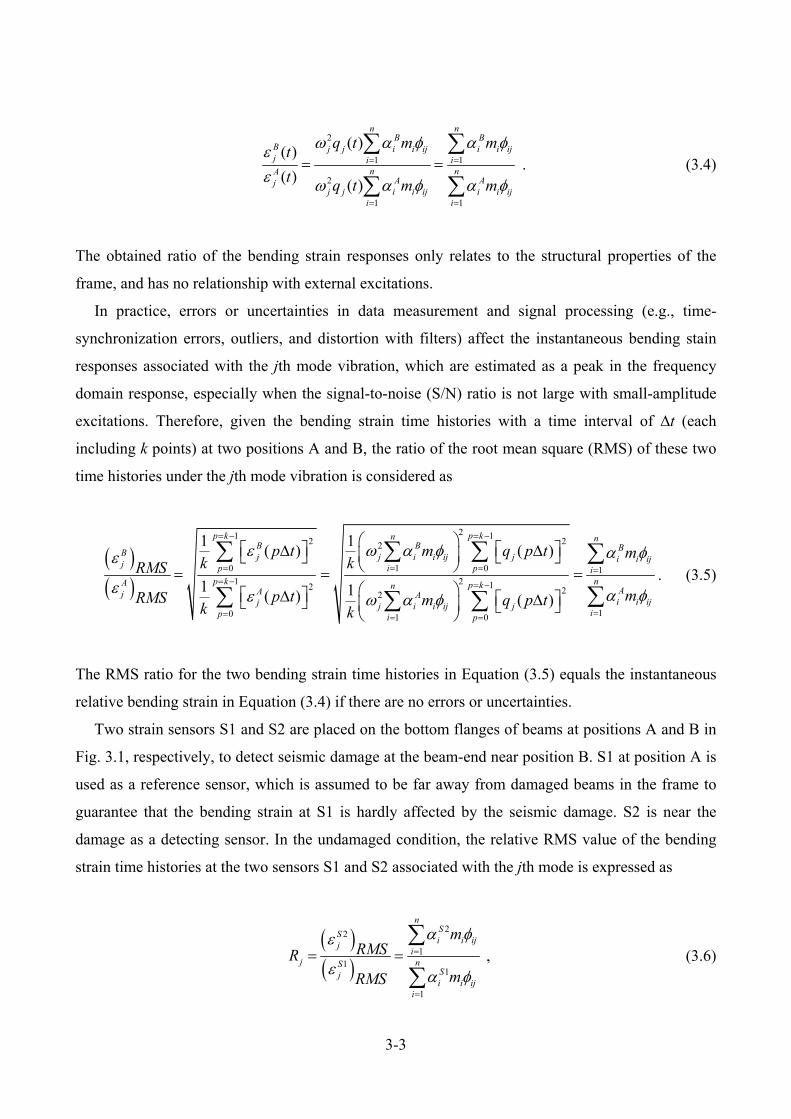
3.3 Signal processing for extracting damage index

In signal processing, the strain time histories associated with a vibration mode is obtained by

applying a narrow-band-pass filter at the frequency of interest as the transient strain responses of

the structural members in the frame are a combination of responses associated with the various

vibration modes of the frame. Fig. 3.2 shows the flowchart of the step-by-step procedure for

calculating the damage index DI. First, raw dynamic strain data of steel beams is preprocessed with

data cleaning techniques (e.g., the removal of drifts and false points). Second, one mode of the steel

moment-resisting frame is selected and the strain responses associated with the selected mode are

extracted using band-pass filters. Third, the RMS values of the filtered strain data are calculated and

then normalized by the RMS value of a reference position. Finally, damage information (existence,

location, and extent) is extracted from the damage index DI calculated in Equation (3.8) at each

detecting sensor.

 

3-5  

Fig. 3.2 Step-by-step procedure to extract damage index

3.4 Five-story steel frame testbed

The performance of the developed local damage evaluation strategy was verified with a steel

frame testbed. The study using a sensing system deployed on a real building is ideal but it is very

rare to acquire an opportunity to simulate damage in buildings. Therefore, a five-story steel frame

testbed that accommodates earthquake-induced fracture at beam ends was constructed at the

Disaster Prevention Research Institute (DPRI), Kyoto University, for promoting structural health

monitoring related studies.

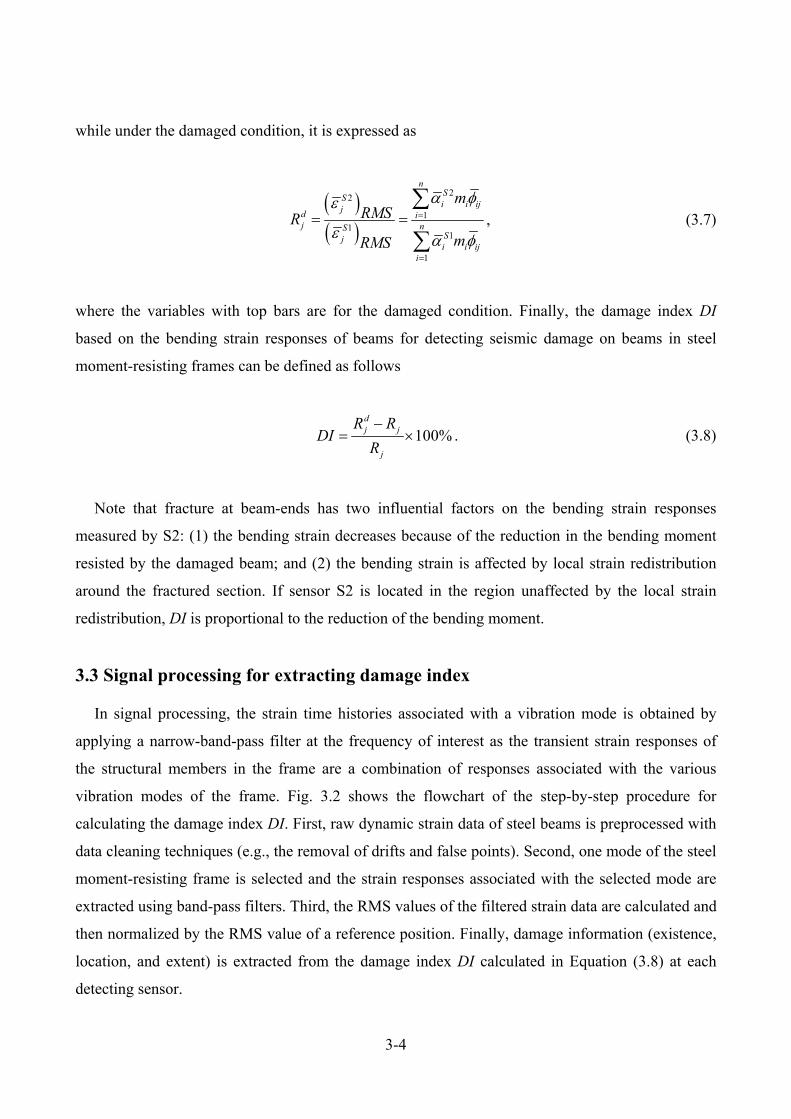
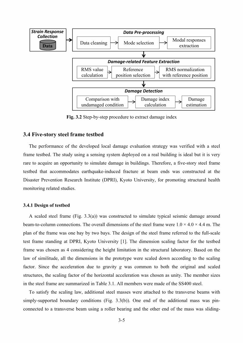
3.4.1 Design of testbed

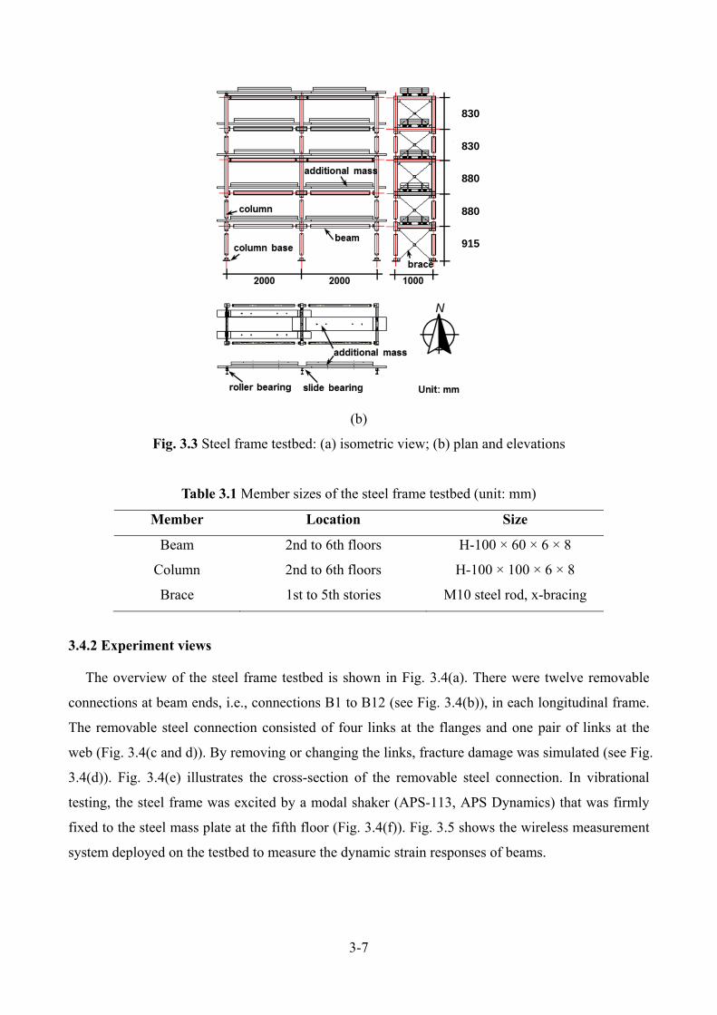
A scaled steel frame (Fig. 3.3(a)) was constructed to simulate typical seismic damage around

beam-to-column connections. The overall dimensions of the steel frame were 1.0 × 4.0 × 4.4 m. The

plan of the frame was one bay by two bays. The design of the steel frame referred to the full-scale

test frame standing at DPRI, Kyoto University [1]. The dimension scaling factor for the testbed

frame was chosen as 4 considering the height limitation in the structural laboratory. Based on the

law of similitude, all the dimensions in the prototype were scaled down according to the scaling

factor. Since the acceleration due to gravity g was common to both the original and scaled

structures, the scaling factor of the horizontal acceleration was chosen as unity. The member sizes

in the steel frame are summarized in Table 3.1. All members were made of the SS400 steel.

To satisfy the scaling law, additional steel masses were attached to the transverse beams with

simply-supported boundary conditions (Fig. 3.3(b)). One end of the additional mass was pin-

connected to a transverse beam using a roller bearing and the other end of the mass was sliding-

Strain Response Collection  

Data

 Data Pre‐processing

Data cleaning Mode selection Modal responses

extraction

 Damage‐related Feature Extraction

RMS value calculation

Reference position selection

RMS normalization with reference position

 

Damage Detection

Comparison with undamaged condition

Damage index calculation

Damage estimation

 

3-6  

supported by a Teflon plate so that the high stiffness of the additional mass did not constrain the

deformation of the longitudinal beams. With the additional mass, the natural frequencies of the

testbed frame became those of the original frame multiplied by the square root of the dimension

scaling factor.

Seismic damage was simulated at the removable steel connections located at the second, third,

and fifth floors. As seen in the enlarged drawing in Fig. 3.3(a), the longitudinal beams in the x

direction and column were connected to a joint using removable steel links and structural bolts. The

dimensions of the steel links were defined so that the second moments of inertia at the removable

connections were equal to those of the connected beams or columns.

(a)

 

3-7  

(b)

Fig. 3.3 Steel frame testbed: (a) isometric view; (b) plan and elevations

Table 3.1 Member sizes of the steel frame testbed (unit: mm)

Member Location Size

Beam 2nd to 6th floors H-100 × 60 × 6 × 8

Column 2nd to 6th floors H-100 × 100 × 6 × 8

Brace 1st to 5th stories M10 steel rod, x-bracing

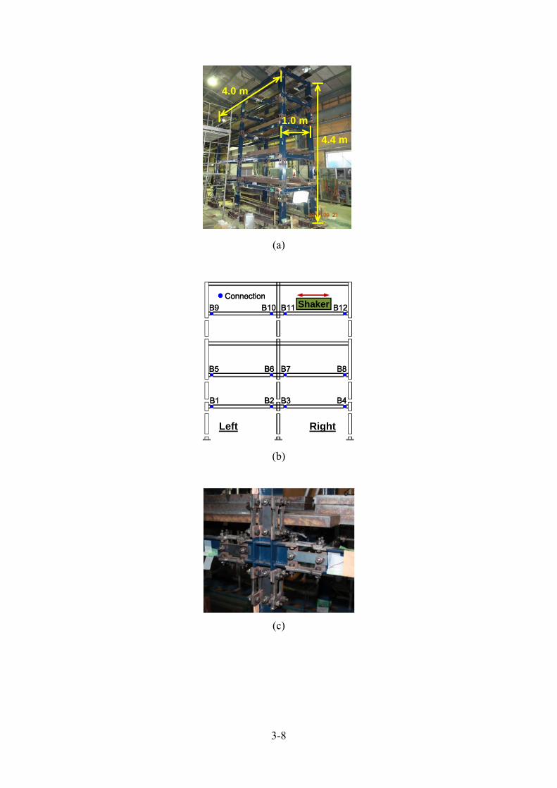
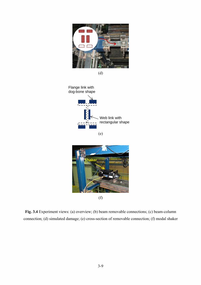
3.4.2 Experiment views

The overview of the steel frame testbed is shown in Fig. 3.4(a). There were twelve removable

connections at beam ends, i.e., connections B1 to B12 (see Fig. 3.4(b)), in each longitudinal frame.

The removable steel connection consisted of four links at the flanges and one pair of links at the

web (Fig. 3.4(c and d)). By removing or changing the links, fracture damage was simulated (see Fig.

3.4(d)). Fig. 3.4(e) illustrates the cross-section of the removable steel connection. In vibrational

testing, the steel frame was excited by a modal shaker (APS-113, APS Dynamics) that was firmly

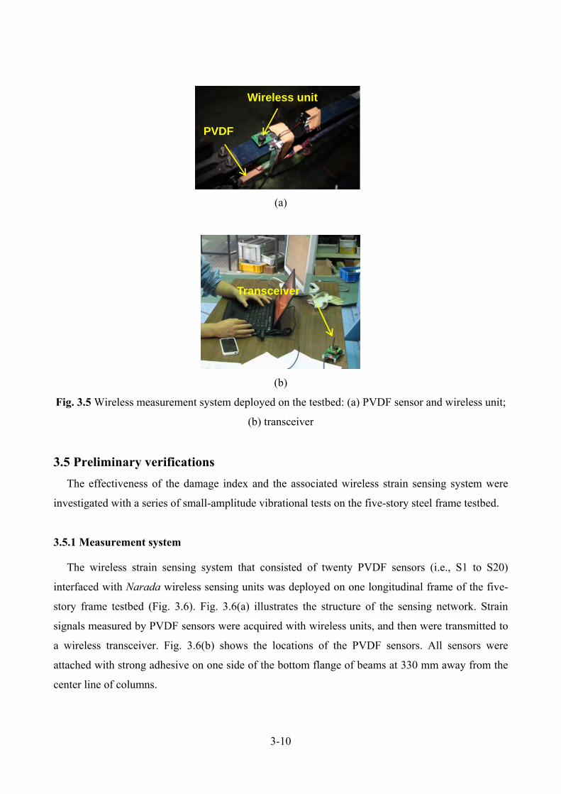
fixed to the steel mass plate at the fifth floor (Fig. 3.4(f)). Fig. 3.5 shows the wireless measurement

system deployed on the testbed to measure the dynamic strain responses of beams.

830

830

880

880

915

 

3-8  

(a)

(b)

(c)

Left Right

Shaker

4.4 m

1.0 m

4.0 m

 

3-9  

(d)

(e)

(f)

Fig. 3.4 Experiment views: (a) overview; (b) beam removable connections; (c) beam-column

connection; (d) simulated damage; (e) cross-section of removable connection; (f) modal shaker

Flange link with dog-bone shape

Web link with rectangular shape

Shaker

 

3-10  

(a)

(b)

Fig. 3.5 Wireless measurement system deployed on the testbed: (a) PVDF sensor and wireless unit;

(b) transceiver

3.5 Preliminary verifications

The effectiveness of the damage index and the associated wireless strain sensing system were

investigated with a series of small-amplitude vibrational tests on the five-story steel frame testbed.

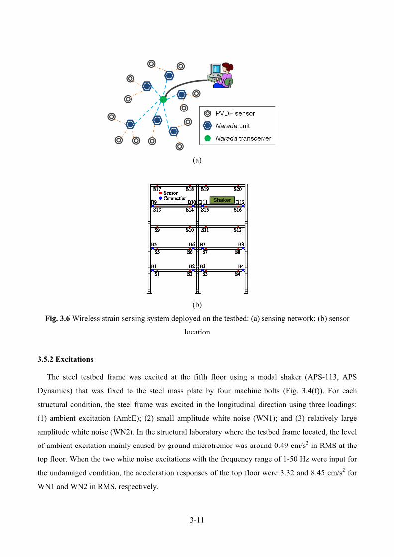
3.5.1 Measurement system

The wireless strain sensing system that consisted of twenty PVDF sensors (i.e., S1 to S20)

interfaced with Narada wireless sensing units was deployed on one longitudinal frame of the five-

story frame testbed (Fig. 3.6). Fig. 3.6(a) illustrates the structure of the sensing network. Strain

signals measured by PVDF sensors were acquired with wireless units, and then were transmitted to

a wireless transceiver. Fig. 3.6(b) shows the locations of the PVDF sensors. All sensors were

attached with strong adhesive on one side of the bottom flange of beams at 330 mm away from the

center line of columns.

Transceiver

Wireless unit

PVDF

 

3-11  

(a)

(b)

Fig. 3.6 Wireless strain sensing system deployed on the testbed: (a) sensing network; (b) sensor

location

3.5.2 Excitations

The steel testbed frame was excited at the fifth floor using a modal shaker (APS-113, APS

Dynamics) that was fixed to the steel mass plate by four machine bolts (Fig. 3.4(f)). For each

structural condition, the steel frame was excited in the longitudinal direction using three loadings:

(1) ambient excitation (AmbE); (2) small amplitude white noise (WN1); and (3) relatively large

amplitude white noise (WN2). In the structural laboratory where the testbed frame located, the level

of ambient excitation mainly caused by ground microtremor was around 0.49 cm/s2 in RMS at the

top floor. When the two white noise excitations with the frequency range of 1-50 Hz were input for

the undamaged condition, the acceleration responses of the top floor were 3.32 and 8.45 cm/s2 for

WN1 and WN2 in RMS, respectively.

PVDF sensor

Narada unit

Narada transceiver

 

Shaker

 

3-12  

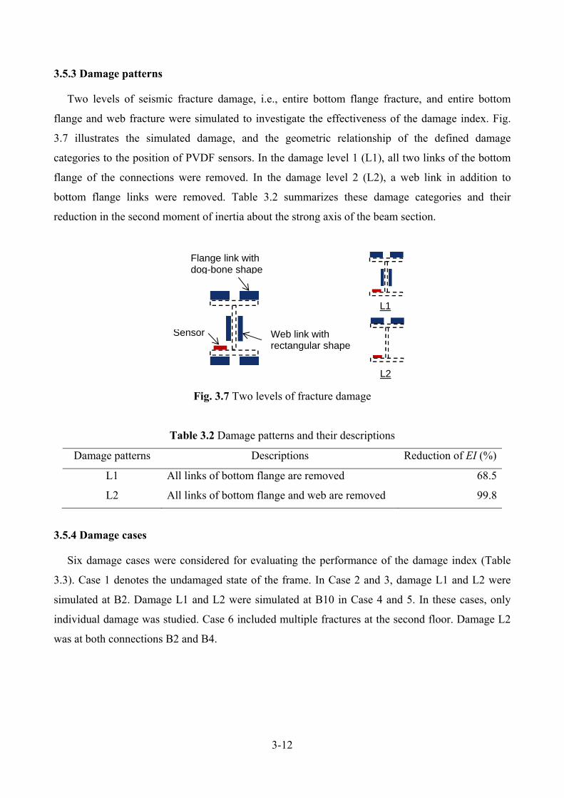
3.5.3 Damage patterns

Two levels of seismic fracture damage, i.e., entire bottom flange fracture, and entire bottom

flange and web fracture were simulated to investigate the effectiveness of the damage index. Fig.

3.7 illustrates the simulated damage, and the geometric relationship of the defined damage

categories to the position of PVDF sensors. In the damage level 1 (L1), all two links of the bottom

flange of the connections were removed. In the damage level 2 (L2), a web link in addition to

bottom flange links were removed. Table 3.2 summarizes these damage categories and their

reduction in the second moment of inertia about the strong axis of the beam section.

Fig. 3.7 Two levels of fracture damage

Table 3.2 Damage patterns and their descriptions

Damage patterns Descriptions Reduction of EI (%)

L1 All links of bottom flange are removed 68.5

L2 All links of bottom flange and web are removed 99.8

3.5.4 Damage cases

Six damage cases were considered for evaluating the performance of the damage index (Table

3.3). Case 1 denotes the undamaged state of the frame. In Case 2 and 3, damage L1 and L2 were

simulated at B2. Damage L1 and L2 were simulated at B10 in Case 4 and 5. In these cases, only

individual damage was studied. Case 6 included multiple fractures at the second floor. Damage L2

was at both connections B2 and B4.

Sensor

Flange link with dog-bone shape

Web link with rectangular shape

L1

L2

 

3-13  

Table 3.3 Damage cases

Damage cases Locations of removable connections and associated damage patterns

Case 1 Undamaged state

Case 2 B2 (L1)

Case 3 B2 (L2)

Case 4 B10 (L1)

Case 5 B10 (L2)

Case 6 B2 (L2), B4 (L2)

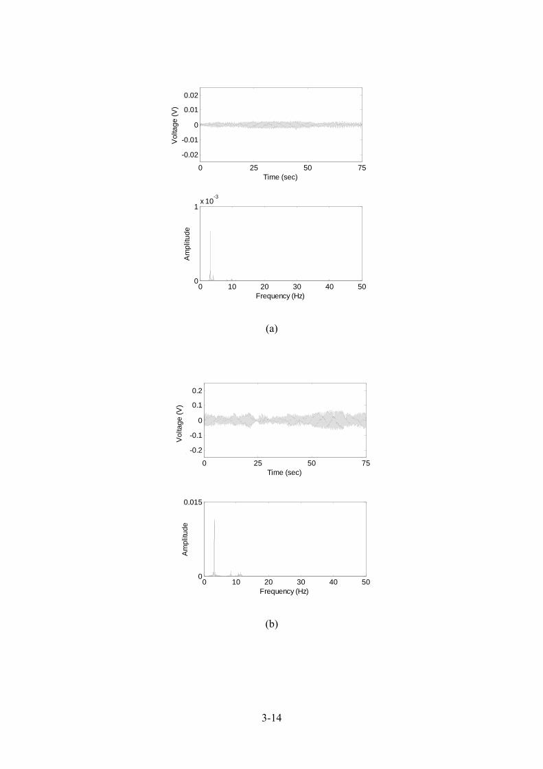
3.5.5 Test results

In each measurement, a strain time history was measured for 75 sec with a sampling rate of 100

Hz. Fig. 3.8 shows the dynamic strain responses at the undamaged condition in voltage and their

amplitude spectra at the beam of the second floor (S2 in Fig. 3.6(b)) under three excitations. The

dynamic characteristics of the testbed frame were evaluated from the floor acceleration responses

under large amplitude white noise excitation (WN2) using the Frequency Domain Decomposition

(FDD) method. The acceleration records were measured at a sampling rate of 100 Hz. The

identified frequencies were 3.16 and 8.33 Hz for the first and second modes in the undamaged

condition, respectively. Compared to the identified two frequencies from acceleration records, the

frequencies of 3.15 and 8.33 Hz obtained from the peaks in the amplitude spectra of the measured

strain responses have differences of less than 0.5%. This indicates that the wireless strain sensing

system was effective and sufficiently sensitive for monitoring strain responses even under ambient

vibrations.

 

3-14  

(a)

(b)

0 25 50 75

-0.02

-0.01

0

0.01

0.02

Time (sec)V

olta

ge

(V

)

0 10 20 30 40 500

1x 10

-3

Frequency (Hz)

Am

plit

ud

e

0 25 50 75

-0.2

-0.1

0

0.1

0.2

Time (sec)

0 10 20 30 40 500

0.015

Frequency (Hz)

-

-Vo

ltag

e (

V)

1

Am

plit

ud

e

 

3-15  

(c)

Fig. 3.8 Measured signals at S2: (a) AmbE; (b) WN1; (c) WN2

The strain response associated with the first mode was used for computing the damage index.

Considering the change in the first mode frequency with relation to the extent of damage, a band-

pass filter of 2.7–3.3 Hz was selected to obtain the dynamic strain associated with the first mode.

Then, the RMS values of each of the filtered strain responses was normalized by the RMS values of

the reference strain data measured at the beam of the top floor (i.e., S20 in Fig. 3.6(b)).

The damage index at all the sensor locations was evaluated for the undamaged condition and the

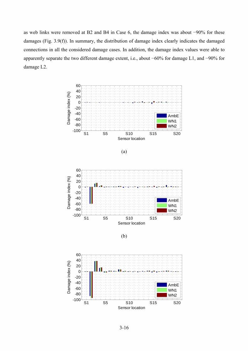
other five damaged cases described in Table 3.3. Fig. 3.9 shows the damage index results for the

undamaged and damaged cases under three different excitations. At the undamaged condition, the

variation of the damage index was less than 7% for all the input excitations (Fig. 3.9(a)). Fig. 3.9(b)

shows the results for Case 2 where the entire bottom flange links were removed at B2 near S2. The

damage index of −60% at S2 clearly indicates the existence of severe damage at B2. In addition, the

damage index of +18% at S3 also indicates damage at nearby connections. Fig. 3.9(c) shows the

results for Case 3 where all the links of the bottom flange and web were removed at B2. With the

removal of both the web and the flange links, the damage index at S2 decreased by 90%, indicating

severe damage at B2. As in Case 2, the damage index at the nearby sensors increased (by 35% at

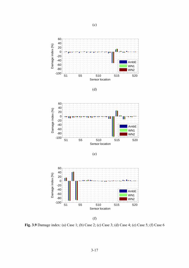
S3). Similarly, the damage index of about −60% and −90% in Case 4 and 5 corresponded to the

damage L1 and L2 at the connection B10 (Fig. 3.9(d and e)). When all bottom flange links as well

0 25 50 75

-0.2

-0.1

0

0.1

0.2

Time (sec)

0 10 20 30 40 500

0.04

Frequency (Hz)

-

-Vo

ltag

e (

V)

1

Am

plit

ud

e

 

3-16  

as web links were removed at B2 and B4 in Case 6, the damage index was about −90% for these

damages (Fig. 3.9(f)). In summary, the distribution of damage index clearly indicates the damaged

connections in all the considered damage cases. In addition, the damage index values were able to

apparently separate the two different damage extent, i.e., about −60% for damage L1, and −90% for

damage L2.

(a)

(b)

S1 S5 S10 S15 S20-100

-80-60

-40-20

020

4060

Sensor location

Dam

ag

e in

dex

(%)

AmbEWN1WN2

S1 S5 S10 S15 S20-100

-80-60

-40-20

020

4060

Sensor location

Dam

ag

e in

dex

(%)

AmbEWN1WN2

S1 S5 S10 S15 S20-100

-80-60

-40-20

020

4060

Sensor location

Dam

ag

e in

dex

(%)

AmbEWN1WN2

 

3-17  

(c)

(d)

(e)

(f)

Fig. 3.9 Damage index: (a) Case 1; (b) Case 2; (c) Case 3; (d) Case 4; (e) Case 5; (f) Case 6

S1 S5 S10 S15 S20-100

-80-60

-40-20

020

4060

Sensor location

Dam

ag

e in

dex

(%)

AmbEWN1WN2

S1 S5 S10 S15 S20-100

-80-60

-40-20

0

204060

Sensor location

Dam

ag

e in

dex

(%)

AmbEWN1WN2

S1 S5 S10 S15 S20-100

-80-60

-40-20

020

4060

Sensor location

Da

ma

ge

ind

ex

(%)

AmbEWN1WN2

 

3-18  

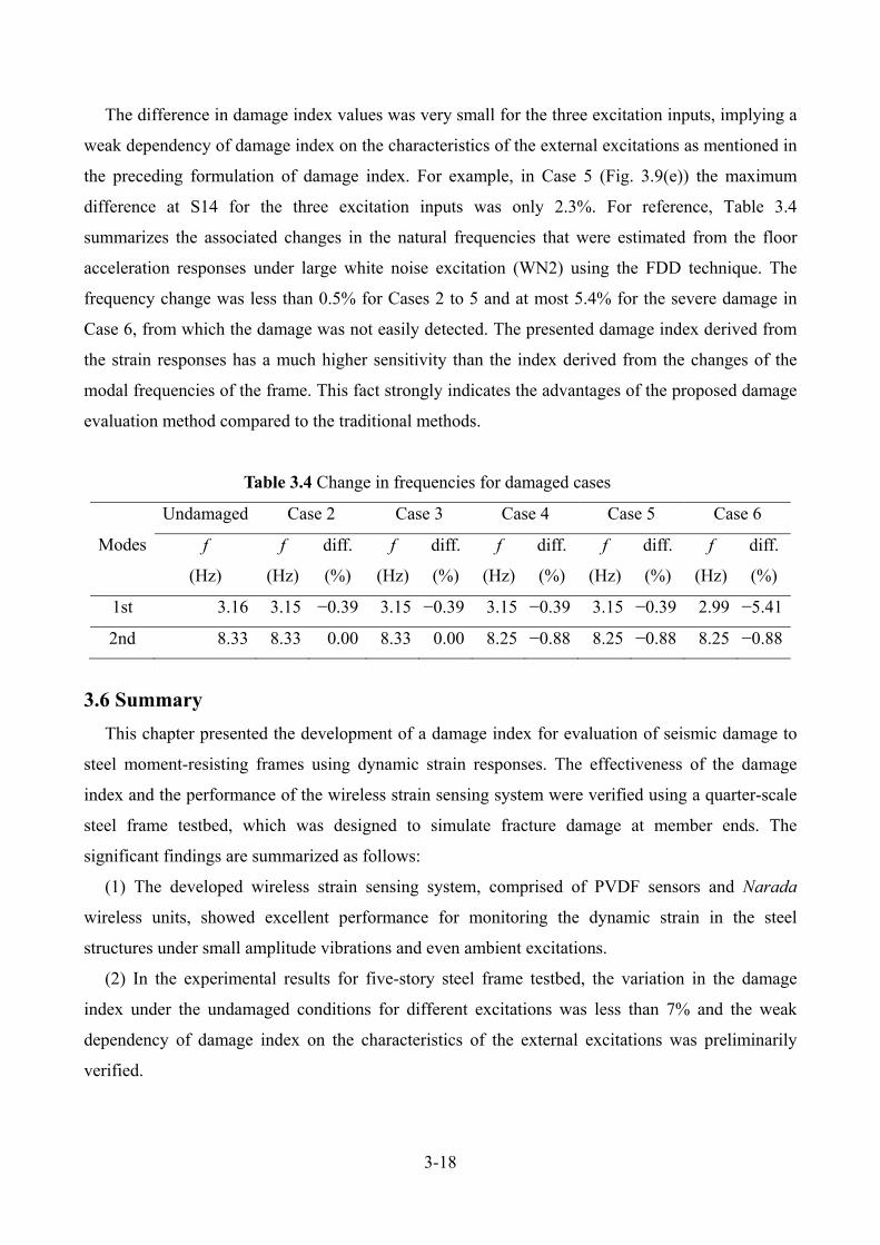
The difference in damage index values was very small for the three excitation inputs, implying a

weak dependency of damage index on the characteristics of the external excitations as mentioned in

the preceding formulation of damage index. For example, in Case 5 (Fig. 3.9(e)) the maximum

difference at S14 for the three excitation inputs was only 2.3%. For reference, Table 3.4

summarizes the associated changes in the natural frequencies that were estimated from the floor

acceleration responses under large white noise excitation (WN2) using the FDD technique. The

frequency change was less than 0.5% for Cases 2 to 5 and at most 5.4% for the severe damage in

Case 6, from which the damage was not easily detected. The presented damage index derived from

the strain responses has a much higher sensitivity than the index derived from the changes of the

modal frequencies of the frame. This fact strongly indicates the advantages of the proposed damage

evaluation method compared to the traditional methods.

Table 3.4 Change in frequencies for damaged cases

Modes

Undamaged Case 2 Case 3 Case 4 Case 5 Case 6

f

(Hz)

f

(Hz)

diff.

(%)

f

(Hz)

diff.

(%)

f

(Hz)

diff.

(%)

f

(Hz)

diff.

(%)

f

(Hz)

diff.

(%)

1st 3.16 3.15 −0.39 3.15 −0.39 3.15 −0.39 3.15 −0.39 2.99 −5.41

2nd 8.33 8.33 0.00 8.33 0.00 8.25 −0.88 8.25 −0.88 8.25 −0.88

3.6 Summary

This chapter presented the development of a damage index for evaluation of seismic damage to

steel moment-resisting frames using dynamic strain responses. The effectiveness of the damage

index and the performance of the wireless strain sensing system were verified using a quarter-scale

steel frame testbed, which was designed to simulate fracture damage at member ends. The

significant findings are summarized as follows:

(1) The developed wireless strain sensing system, comprised of PVDF sensors and Narada

wireless units, showed excellent performance for monitoring the dynamic strain in the steel

structures under small amplitude vibrations and even ambient excitations.

(2) In the experimental results for five-story steel frame testbed, the variation in the damage

index under the undamaged conditions for different excitations was less than 7% and the weak

dependency of damage index on the characteristics of the external excitations was preliminarily

verified.

 

3-19  

(3) The damaged locations were successfully identified in the tests using the distribution of

damage index values. Moreover, the damage index values for the various severity levels showed

clear discrete values that would enable the quantification of seismic fracture damage.

REFERENCES

[1] Iemura. H., Igarashi, A., Fujiwara, T., and Toyooka, A. (2000). Full-scale Verification Test of

Dynamic Response Control Techniques for Strong Earthquakes, the Proceedings of 12th

World Conference of Earthquake Engineering, 1795.

 

3-20  

 

4-1  

CHAPTER 4

Sensitivity investigation of strain-based damage index

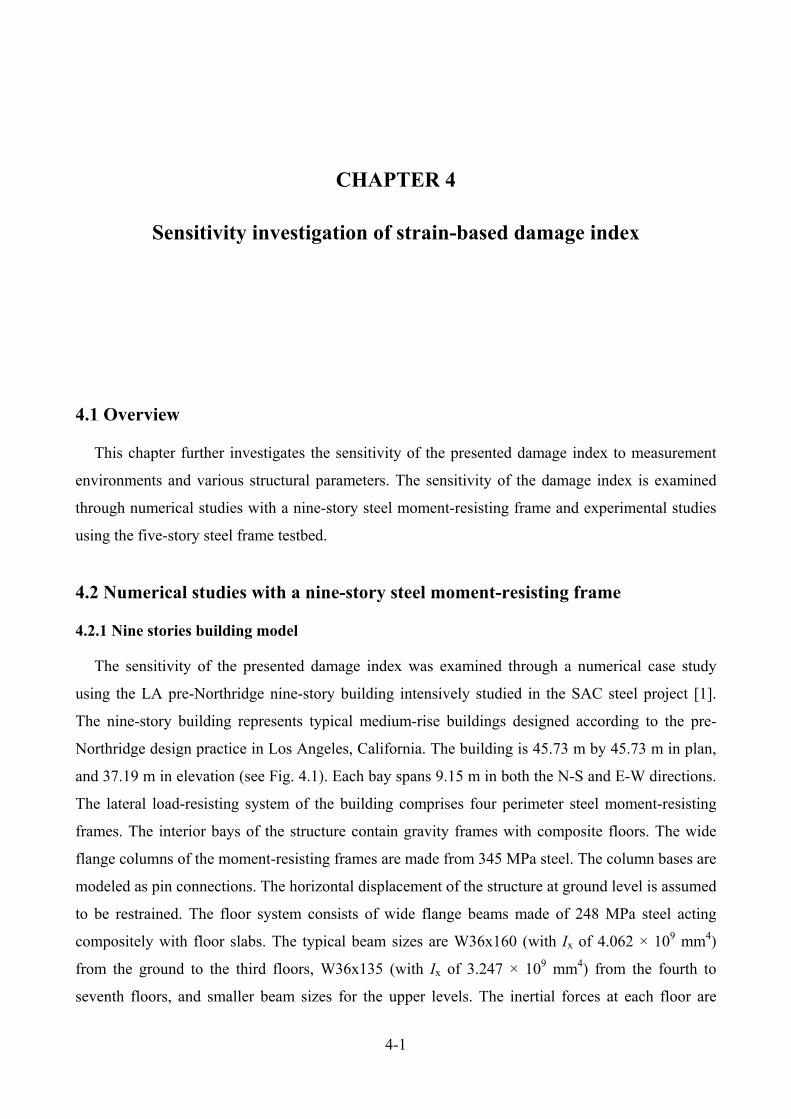
4.1 Overview

This chapter further investigates the sensitivity of the presented damage index to measurement

environments and various structural parameters. The sensitivity of the damage index is examined

through numerical studies with a nine-story steel moment-resisting frame and experimental studies

using the five-story steel frame testbed.

4.2 Numerical studies with a nine-story steel moment-resisting frame

4.2.1 Nine stories building model

The sensitivity of the presented damage index was examined through a numerical case study

using the LA pre-Northridge nine-story building intensively studied in the SAC steel project [1].

The nine-story building represents typical medium-rise buildings designed according to the pre-

Northridge design practice in Los Angeles, California. The building is 45.73 m by 45.73 m in plan,

and 37.19 m in elevation (see Fig. 4.1). Each bay spans 9.15 m in both the N-S and E-W directions.

The lateral load-resisting system of the building comprises four perimeter steel moment-resisting

frames. The interior bays of the structure contain gravity frames with composite floors. The wide

flange columns of the moment-resisting frames are made from 345 MPa steel. The column bases are

modeled as pin connections. The horizontal displacement of the structure at ground level is assumed

to be restrained. The floor system consists of wide flange beams made of 248 MPa steel acting

compositely with floor slabs. The typical beam sizes are W36x160 (with Ix of 4.062 × 109 mm4)

from the ground to the third floors, W36x135 (with Ix of 3.247 × 109 mm4) from the fourth to

seventh floors, and smaller beam sizes for the upper levels. The inertial forces at each floor are

 

4-2  

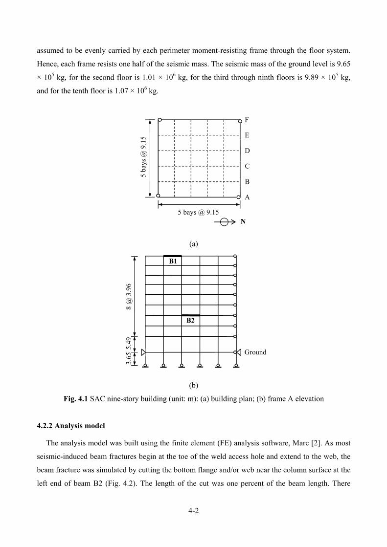
assumed to be evenly carried by each perimeter moment-resisting frame through the floor system.

Hence, each frame resists one half of the seismic mass. The seismic mass of the ground level is 9.65

× 105 kg, for the second floor is 1.01 × 106 kg, for the third through ninth floors is 9.89 × 105 kg,

and for the tenth floor is 1.07 × 106 kg.

(a)

(b)

Fig. 4.1 SAC nine-story building (unit: m): (a) building plan; (b) frame A elevation

4.2.2 Analysis model

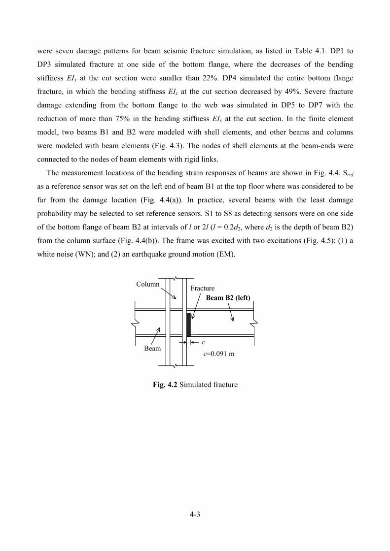
The analysis model was built using the finite element (FE) analysis software, Marc [2]. As most

seismic-induced beam fractures begin at the toe of the weld access hole and extend to the web, the

beam fracture was simulated by cutting the bottom flange and/or web near the column surface at the

left end of beam B2 (Fig. 4.2). The length of the cut was one percent of the beam length. There

5 ba

ys @

9.1

5

5 bays @ 9.15

A

B

C

D

E

F

N

3.65

5.4

9 8

@ 3

.96

Ground

B1

B2

 

4-3  

were seven damage patterns for beam seismic fracture simulation, as listed in Table 4.1. DP1 to

DP3 simulated fracture at one side of the bottom flange, where the decreases of the bending

stiffness EIx at the cut section were smaller than 22%. DP4 simulated the entire bottom flange

fracture, in which the bending stiffness EIx at the cut section decreased by 49%. Severe fracture

damage extending from the bottom flange to the web was simulated in DP5 to DP7 with the

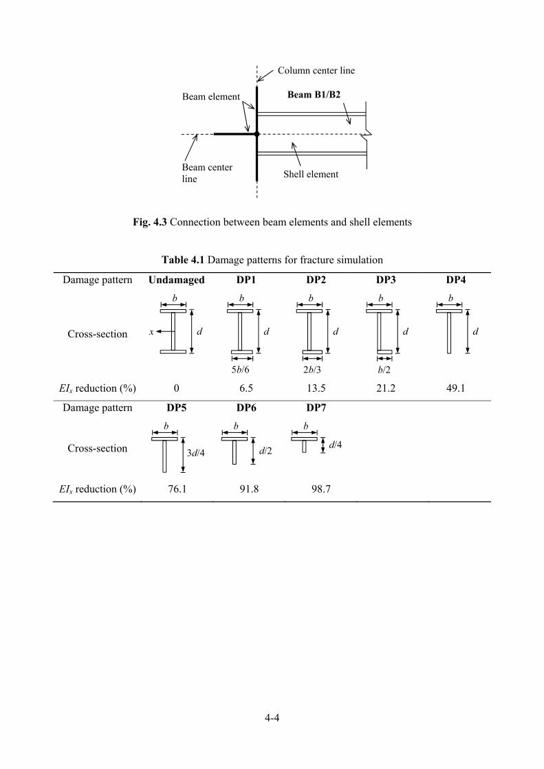
reduction of more than 75% in the bending stiffness EIx at the cut section. In the finite element

model, two beams B1 and B2 were modeled with shell elements, and other beams and columns

were modeled with beam elements (Fig. 4.3). The nodes of shell elements at the beam-ends were

connected to the nodes of beam elements with rigid links.

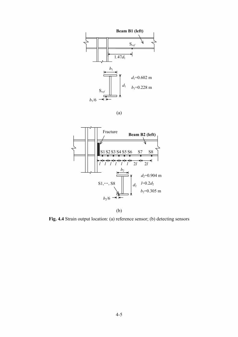
The measurement locations of the bending strain responses of beams are shown in Fig. 4.4. Sref

as a reference sensor was set on the left end of beam B1 at the top floor where was considered to be

far from the damage location (Fig. 4.4(a)). In practice, several beams with the least damage

probability may be selected to set reference sensors. S1 to S8 as detecting sensors were on one side

of the bottom flange of beam B2 at intervals of l or 2l (l = 0.2d2, where d2 is the depth of beam B2)

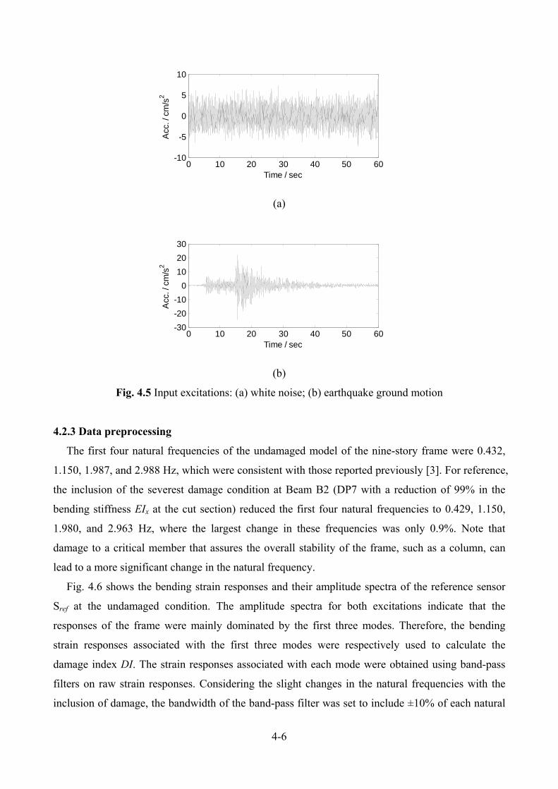
from the column surface (Fig. 4.4(b)). The frame was excited with two excitations (Fig. 4.5): (1) a

white noise (WN); and (2) an earthquake ground motion (EM).

Fig. 4.2 Simulated fracture

Column

Beam B2 (left)

 

c

Fracture

c=0.091 mBeam

 

4-4  

Fig. 4.3 Connection between beam elements and shell elements

Table 4.1 Damage patterns for fracture simulation

Damage pattern Undamaged DP1 DP2 DP3 DP4

Cross-section

EIx reduction (%) 0 6.5 13.5 21.2 49.1

Damage pattern DP5 DP6 DP7

Cross-section

EIx reduction (%) 76.1 91.8 98.7

Column center line

Beam B1/B2

Beam center line

Beam element

Shell element

 

b

d x 

b

d

5b/6

 

b

d

2b/3

 

b

d

b/2

 

b

d

 

b

3d/4  

b

d/2

b

d/4

 

4-5  

(a)

(b)

Fig. 4.4 Strain output location: (a) reference sensor; (b) detecting sensors

1.47d1

Beam B1 (left)

Sref

d1=0.602 m

b1=0.228 m

 

Sref

b1

b1/6

d1

Beam B2 (left)

S1

l

Fracture

d2=0.904 m

b2=0.305 m

S2 S3 S4 S5 S6 S7 S8

l l l ll 2l2lb2

b2/6

S1,…,S8 d2l=0.2d2

 

 

4-6  

(a)

(b)

Fig. 4.5 Input excitations: (a) white noise; (b) earthquake ground motion

4.2.3 Data preprocessing

The first four natural frequencies of the undamaged model of the nine-story frame were 0.432,

1.150, 1.987, and 2.988 Hz, which were consistent with those reported previously [3]. For reference,

the inclusion of the severest damage condition at Beam B2 (DP7 with a reduction of 99% in the

bending stiffness EIx at the cut section) reduced the first four natural frequencies to 0.429, 1.150,

1.980, and 2.963 Hz, where the largest change in these frequencies was only 0.9%. Note that

damage to a critical member that assures the overall stability of the frame, such as a column, can

lead to a more significant change in the natural frequency.

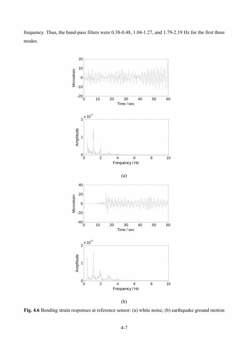
Fig. 4.6 shows the bending strain responses and their amplitude spectra of the reference sensor

Sref at the undamaged condition. The amplitude spectra for both excitations indicate that the

responses of the frame were mainly dominated by the first three modes. Therefore, the bending

strain responses associated with the first three modes were respectively used to calculate the

damage index DI. The strain responses associated with each mode were obtained using band-pass

filters on raw strain responses. Considering the slight changes in the natural frequencies with the

inclusion of damage, the bandwidth of the band-pass filter was set to include ±10% of each natural

0 10 20 30 40 50 60-10

-5

0

5

10

Time / secA

cc. /

cm

/s2

0 10 20 30 40 50 60-30

-20

-10

0

10

20

30

Time / sec

Acc

. / c

m/s

2

 

4-7  

frequency. Thus, the band-pass filters were 0.38-0.48, 1.04-1.27, and 1.79-2.19 Hz for the first three

modes.

(a)

(b)

Fig. 4.6 Bending strain responses at reference sensor: (a) white noise; (b) earthquake ground motion

0 10 20 30 40 50 60-20

-10

0

10

20

Time / sec

Mic

rost

rain

0 2 4 6 8 100

1

2x 10

-6

Frequency / Hz

Am

plitu

de

0 10 20 30 40 50 60-40

-20

0

20

40

Time / sec

Mic

rost

rain

0 2 4 6 8 100

1

2x 10

-6

Frequency / Hz

Am

plitu

de

 

4-8  

4.2.4 Simulation results

The sensitivity of the presented damage index to input excitation, vibrational mode, the selection

of reference data, and sensor location were studied using the constructed analysis model.

4.2.4.1 Independency on excitations and modes

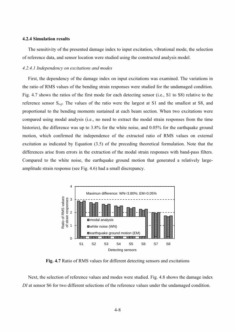
First, the dependency of the damage index on input excitations was examined. The variations in

the ratio of RMS values of the bending strain responses were studied for the undamaged condition.

Fig. 4.7 shows the ratios of the first mode for each detecting sensor (i.e., S1 to S8) relative to the

reference sensor Sref. The values of the ratio were the largest at S1 and the smallest at S8, and

proportional to the bending moments sustained at each beam section. When two excitations were

compared using modal analysis (i.e., no need to extract the modal strain responses from the time

histories), the difference was up to 3.8% for the white noise, and 0.05% for the earthquake ground

motion, which confirmed the independence of the extracted ratio of RMS values on external

excitation as indicated by Equation (3.5) of the preceding theoretical formulation. Note that the

differences arise from errors in the extraction of the modal strain responses with band-pass filters.

Compared to the white noise, the earthquake ground motion that generated a relatively large-

amplitude strain response (see Fig. 4.6) had a small discrepancy.

Fig. 4.7 Ratio of RMS values for different detecting sensors and excitations

Next, the selection of reference values and modes were studied. Fig. 4.8 shows the damage index

DI at sensor S6 for two different selections of the reference values under the undamaged condition.

0

1

2

3

4

S1 S2 S3 S4 S5 S6 S7 S8

Rat

io o

f RM

S v

alue

sof

str

ain

resp

onse

s

Detecting sensors

Maximun difference: WN=3.80%; EM=0.05%

modal analysis

white noise (WN)

earthquake ground motion (EM)

 

4-9  

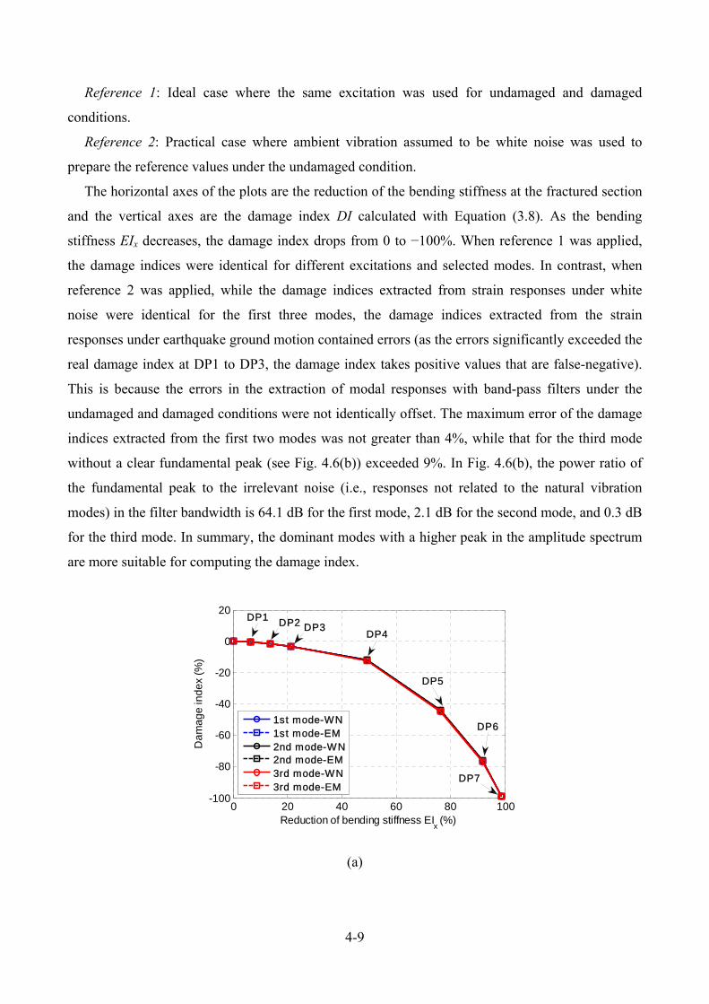
Reference 1: Ideal case where the same excitation was used for undamaged and damaged

conditions.

Reference 2: Practical case where ambient vibration assumed to be white noise was used to

prepare the reference values under the undamaged condition.

The horizontal axes of the plots are the reduction of the bending stiffness at the fractured section

and the vertical axes are the damage index DI calculated with Equation (3.8). As the bending

stiffness EIx decreases, the damage index drops from 0 to −100%. When reference 1 was applied,

the damage indices were identical for different excitations and selected modes. In contrast, when

reference 2 was applied, while the damage indices extracted from strain responses under white

noise were identical for the first three modes, the damage indices extracted from the strain

responses under earthquake ground motion contained errors (as the errors significantly exceeded the

real damage index at DP1 to DP3, the damage index takes positive values that are false-negative).

This is because the errors in the extraction of modal responses with band-pass filters under the

undamaged and damaged conditions were not identically offset. The maximum error of the damage

indices extracted from the first two modes was not greater than 4%, while that for the third mode

without a clear fundamental peak (see Fig. 4.6(b)) exceeded 9%. In Fig. 4.6(b), the power ratio of

the fundamental peak to the irrelevant noise (i.e., responses not related to the natural vibration

modes) in the filter bandwidth is 64.1 dB for the first mode, 2.1 dB for the second mode, and 0.3 dB

for the third mode. In summary, the dominant modes with a higher peak in the amplitude spectrum

are more suitable for computing the damage index.

(a)

0 20 40 60 80 100-100

-80

-60

-40

-20

0

20

Reduction of bending stiffness EIx (%)

Da

ma

ge

ind

ex

(%)

1st mode-WN1st mode-EM2nd mode-WN2nd mode-EM3rd mode-WN3rd mode-EM

DP5

DP2DP1DP3

DP4

DP6

DP7

 

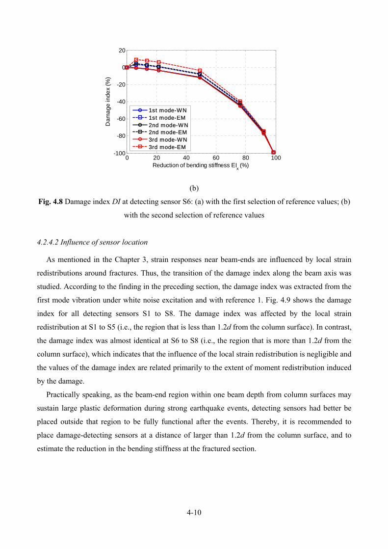
4-10  

(b)

Fig. 4.8 Damage index DI at detecting sensor S6: (a) with the first selection of reference values; (b)

with the second selection of reference values

4.2.4.2 Influence of sensor location

As mentioned in the Chapter 3, strain responses near beam-ends are influenced by local strain

redistributions around fractures. Thus, the transition of the damage index along the beam axis was

studied. According to the finding in the preceding section, the damage index was extracted from the

first mode vibration under white noise excitation and with reference 1. Fig. 4.9 shows the damage

index for all detecting sensors S1 to S8. The damage index was affected by the local strain

redistribution at S1 to S5 (i.e., the region that is less than 1.2d from the column surface). In contrast,

the damage index was almost identical at S6 to S8 (i.e., the region that is more than 1.2d from the

column surface), which indicates that the influence of the local strain redistribution is negligible and

the values of the damage index are related primarily to the extent of moment redistribution induced

by the damage.

Practically speaking, as the beam-end region within one beam depth from column surfaces may

sustain large plastic deformation during strong earthquake events, detecting sensors had better be

placed outside that region to be fully functional after the events. Thereby, it is recommended to

place damage-detecting sensors at a distance of larger than 1.2d from the column surface, and to

estimate the reduction in the bending stiffness at the fractured section.

0 20 40 60 80 100-100

-80

-60

-40

-20

0

20

Reduction of bending stiffness EIx (%)

Da

ma

ge

ind

ex

(%)

1st mode-WN1st mode-EM2nd mode-WN2nd mode-EM3rd mode-WN3rd mode-EM

 

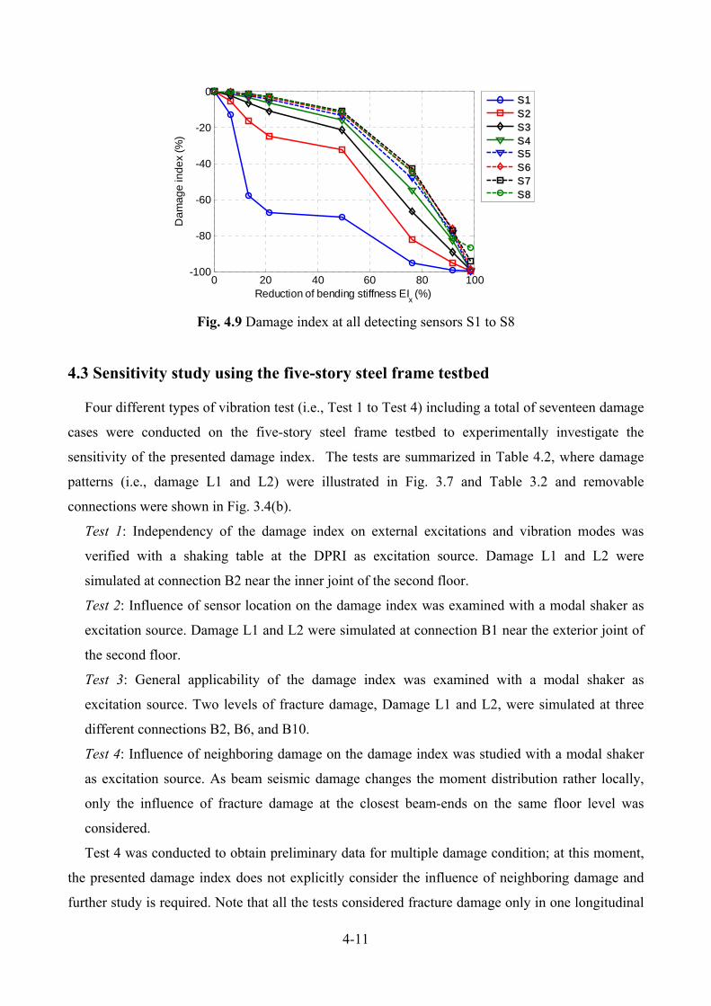
4-11  

Fig. 4.9 Damage index at all detecting sensors S1 to S8

4.3 Sensitivity study using the five-story steel frame testbed

Four different types of vibration test (i.e., Test 1 to Test 4) including a total of seventeen damage

cases were conducted on the five-story steel frame testbed to experimentally investigate the

sensitivity of the presented damage index.  The tests are summarized in Table 4.2, where damage

patterns (i.e., damage L1 and L2) were illustrated in Fig. 3.7 and Table 3.2 and removable

connections were shown in Fig. 3.4(b).

Test 1: Independency of the damage index on external excitations and vibration modes was

verified with a shaking table at the DPRI as excitation source. Damage L1 and L2 were

simulated at connection B2 near the inner joint of the second floor.

Test 2: Influence of sensor location on the damage index was examined with a modal shaker as

excitation source. Damage L1 and L2 were simulated at connection B1 near the exterior joint of

the second floor.

Test 3: General applicability of the damage index was examined with a modal shaker as

excitation source. Two levels of fracture damage, Damage L1 and L2, were simulated at three

different connections B2, B6, and B10.

Test 4: Influence of neighboring damage on the damage index was studied with a modal shaker

as excitation source. As beam seismic damage changes the moment distribution rather locally,

only the influence of fracture damage at the closest beam-ends on the same floor level was

considered.

Test 4 was conducted to obtain preliminary data for multiple damage condition; at this moment,

the presented damage index does not explicitly consider the influence of neighboring damage and

further study is required. Note that all the tests considered fracture damage only in one longitudinal

0 20 40 60 80 100-100

-80

-60

-40

-20

0

Reduction of bending stiffness EIx (%)

Da

ma

ge

ind

ex

(%)

S1S2S3S4S5S6S7S8

 

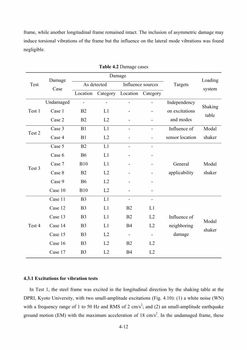
4-12  

frame, while another longitudinal frame remained intact. The inclusion of asymmetric damage may

induce torsional vibrations of the frame but the influence on the lateral mode vibrations was found

negligible.

Table 4.2 Damage cases

Test Damage

Case

Damage

Targets Loading

system As detected Influence sources

Location Category Location Category

Test 1

Undamaged - - - - Independency

on excitations

and modes

Shaking

table Case 1 B2 L1 - -

Case 2 B2 L2 - -

Test 2 Case 3 B1 L1 - - Influence of

sensor location

Modal

shaker Case 4 B1 L2 - -

Test 3

Case 5 B2 L1 - -

General

applicability

Modal

shaker

Case 6 B6 L1 - -

Case 7 B10 L1 - -

Case 8 B2 L2 - -

Case 9 B6 L2 - -

Case 10 B10 L2 - -

Test 4

Case 11 B3 L1 - -

Influence of

neighboring

damage

Modal

shaker

Case 12 B3 L1 B2 L1

Case 13 B3 L1 B2 L2

Case 14 B3 L1 B4 L2

Case 15 B3 L2 - -

Case 16 B3 L2 B2 L2

Case 17 B3 L2 B4 L2

4.3.1 Excitations for vibration tests

In Test 1, the steel frame was excited in the longitudinal direction by the shaking table at the

DPRI, Kyoto University, with two small-amplitude excitations (Fig. 4.10): (1) a white noise (WN)

with a frequency range of 1 to 50 Hz and RMS of 2 cm/s2; and (2) an small-amplitude earthquake

ground motion (EM) with the maximum acceleration of 18 cm/s2. In the undamaged frame, these

 

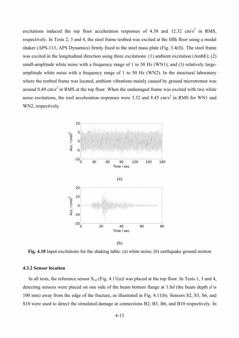
4-13  

excitations induced the top floor acceleration responses of 4.38 and 12.32 cm/s2 in RMS,

respectively. In Tests 2, 3 and 4, the steel frame testbed was excited at the fifth floor using a modal

shaker (APS-113, APS Dynamics) firmly fixed to the steel mass plate (Fig. 3.4(f)). The steel frame

was excited in the longitudinal direction using three excitations: (1) ambient excitation (AmbE); (2)

small-amplitude white noise with a frequency range of 1 to 50 Hz (WN1); and (3) relatively large-

amplitude white noise with a frequency range of 1 to 50 Hz (WN2). In the structural laboratory

where the testbed frame was located, ambient vibrations mainly caused by ground microtremor was

around 0.49 cm/s2 in RMS at the top floor. When the undamaged frame was excited with two white

noise excitations, the roof acceleration responses were 3.32 and 8.45 cm/s2 in RMS for WN1 and

WN2, respectively.

(a)

(b)

Fig. 4.10 Input excitations for the shaking table: (a) white noise; (b) earthquake ground motion

4.3.2 Sensor location

In all tests, the reference sensor Sref (Fig. 4.11(a)) was placed at the top floor. In Tests 1, 3 and 4,

detecting sensors were placed on one side of the beam bottom flange at 1.0d (the beam depth d is

100 mm) away from the edge of the fracture, as illustrated in Fig. 4.11(b). Sensors S2, S3, S6, and

S10 were used to detect the simulated damage at connections B2, B3, B6, and B10 respectively. In

0 30 60 90 120 150 180-10

-5

0

5

10

Time / sec

Acc

. / c

m/s

2

0 20 40 60 80-20

-10

0

10

20

Time / sec

Acc

. / c

m/s

2

 

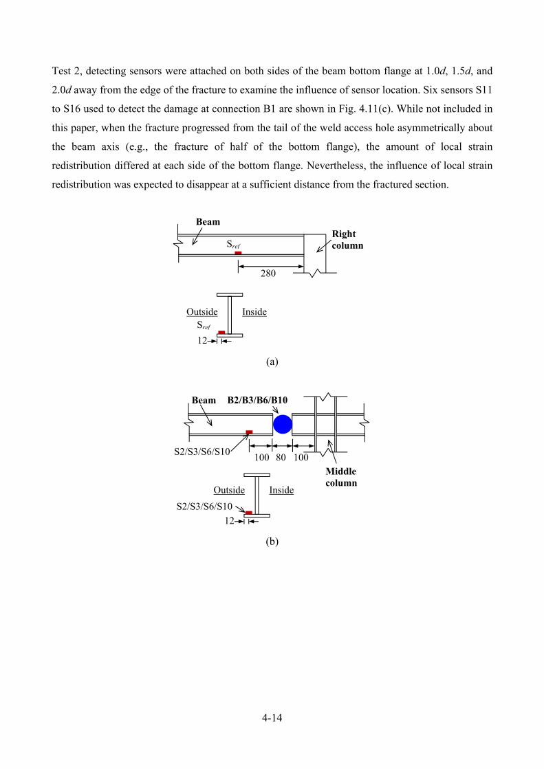
4-14  

Test 2, detecting sensors were attached on both sides of the beam bottom flange at 1.0d, 1.5d, and

2.0d away from the edge of the fracture to examine the influence of sensor location. Six sensors S11

to S16 used to detect the damage at connection B1 are shown in Fig. 4.11(c). While not included in

this paper, when the fracture progressed from the tail of the weld access hole asymmetrically about

the beam axis (e.g., the fracture of half of the bottom flange), the amount of local strain

redistribution differed at each side of the bottom flange. Nevertheless, the influence of local strain

redistribution was expected to disappear at a sufficient distance from the fractured section.

(a)

(b)

280

Right column

Beam

Sref

Outside  

12

InsideSref

100Middle column

Beam

S2/S3/S6/S1080 100

Outside  

12

Inside

B2/B3/B6/B10

S2/S3/S6/S10

 

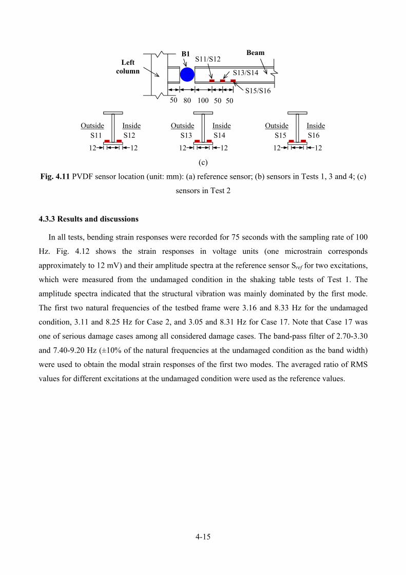
4-15  

(c)

Fig. 4.11 PVDF sensor location (unit: mm): (a) reference sensor; (b) sensors in Tests 1, 3 and 4; (c)

sensors in Test 2

4.3.3 Results and discussions

In all tests, bending strain responses were recorded for 75 seconds with the sampling rate of 100

Hz. Fig. 4.12 shows the strain responses in voltage units (one microstrain corresponds

approximately to 12 mV) and their amplitude spectra at the reference sensor Sref for two excitations,

which were measured from the undamaged condition in the shaking table tests of Test 1. The

amplitude spectra indicated that the structural vibration was mainly dominated by the first mode.

The first two natural frequencies of the testbed frame were 3.16 and 8.33 Hz for the undamaged

condition, 3.11 and 8.25 Hz for Case 2, and 3.05 and 8.31 Hz for Case 17. Note that Case 17 was

one of serious damage cases among all considered damage cases. The band-pass filter of 2.70-3.30

and 7.40-9.20 Hz (±10% of the natural frequencies at the undamaged condition as the band width)

were used to obtain the modal strain responses of the first two modes. The averaged ratio of RMS

values for different excitations at the undamaged condition were used as the reference values.

Outside  

12

Inside S11

12

S12 Outside  

12

InsideS13

12

S14Outside  

12

Inside S15

12

S16

Left column

BeamS11/S12

50 80 100 50 50

S13/S14

S15/S16

B1

 

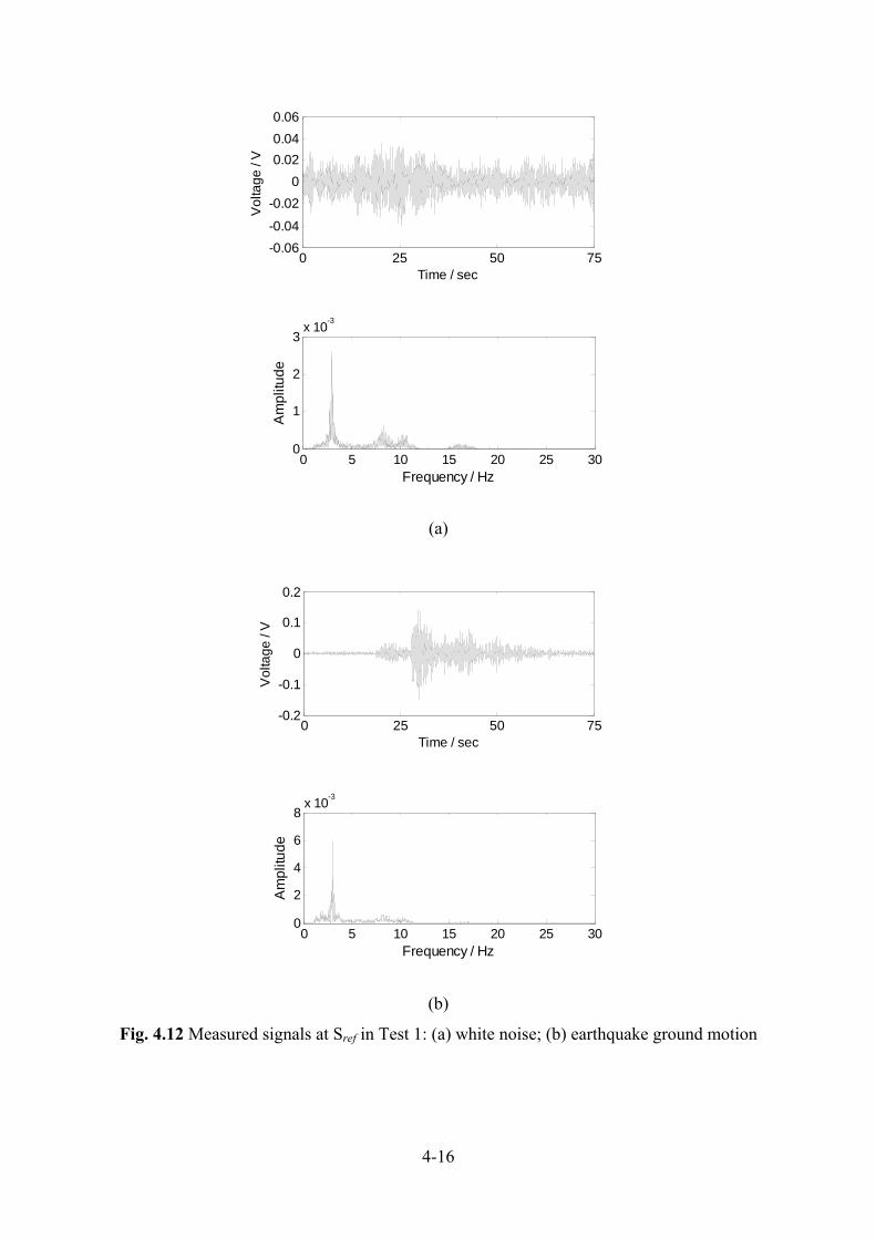
4-16  

(a)

(b)

Fig. 4.12 Measured signals at Sref in Test 1: (a) white noise; (b) earthquake ground motion

0 25 50 75-0.06

-0.04

-0.02

0

0.02

0.04

0.06

Time / sec

Vo

ltag

e /

V

0 5 10 15 20 25 300

1

2

3x 10

-3

Frequency / Hz

Am

plitu

de

0 25 50 75-0.2

-0.1

0

0.1

0.2

Time / sec

Vo

ltag

e /

V

0 5 10 15 20 25 300

2

4

6

8x 10

-3

Frequency / Hz

Am

plitu

de

 

4-17  

4.3.3.1 Test 1

Fig. 4.13 shows the ratios of RMS values of strain responses between sensor S2 and reference

sensor Sref for the first mode. The largest difference in the ratio values between the two different

excitations was 0.78%, which verified independency of the extracted ratio on external excitations as

observed in the preceding theoretical formulation and numerical simulations.

The damage indices of sensor S2 for detecting damage L1 and L2 at connection B2 are

summarized in Table 4.3. In Case 1 with damage L1, i.e., entire bottom flange fracture with the

reduction of 68.5% in the bending stiffness, the damage indices were about −60% for both

excitations with the use of the first mode vibrations but changed to −70% with the use of the second

mode vibrations. Compared to the damage index extracted from the first mode, the damage index of

the second mode had larger discrepancy as the modal strain responses were weak and unclear (see

Fig. 4.12). In Case 2 with damage L2, i.e., entire bottom flange and web fracture with the decrease

of 99.8% in the bending stiffness, the damage indices were smaller than −90% for two excitations

with the first mode vibrations and slightly decreased with the second mode vibrations. As a result,

the dominant modes with clear modal responses and high S/N ratios are highly desirable to increase

the accuracy of the calculation of damage index.

4.3.3.2 Test 2

Table 4.4 summarizes the results of Test 2 for different sensor locations. When damage L1 was

considered at connection B1 in Case 3, the damage indices at sensors S11 and S12, both placed at

100 mm (i.e., the beam depth) away from the edge of the fracture, were about −50%, whereas the

damage indices at sensors S13 and S14, both at 150 mm (i.e., one and half beam depths) away from

the edge, were around −35% to −37%. The damage indices at sensors S15 and S16, both attached at

200 mm (i.e., two beam depths) away from the edge, were −32% to −36% and consistent with those

at S13 and S14. When damage L2 was considered at connection B1 in Case 4, the damage index at

the six sensors S11 to S16 was less than −85%. Compared to the damage index of about −95% at

sensors S11 and S12, the damage index at sensors S13 to S16 had slight changes of 10%, which was

consistent with the findings in the preceding numerical simulations for severe damage DP7; strain

sensors needed to be set within two beam depths to guarantee the monotonic relation between the

damage index and the reduction of bending stiffness. Note that the values at the different sides of

the flange (e.g., S13 and S14, and S15 and S16) varied by 5% with beam torsional vibrations

observed when web links were removed. In conclusion, in order to obtain a stable relation between

the damage index and the reduction of bending stiffness, like the damage index curves for sensors

 

4-18  

S6 to S8 in Fig. 4.9, detecting sensors need to be placed with the distance of at least 1.5d but no

farther than 2.0d from fracture damage as recommended by the previous simulations using the SAC

nine-story frame.

Fig. 4.13 Ratio of RMS of strain responses at S2 and Sref for the first mode in Test 1

Table 4.3 Damage index for detecting damage at connection B2 in Test 1

Mode Excitation Damage index (%)

Undamaged Case 1 Case 2

1st mode WN 0.0 -59.5 -93.5

EM 0.0 -59.7 -93.4

2nd mode WN -1.0 -68.9 -96.5

EM 1.0 -68.4 -96.7

Table 4.4 Damage index for detecting damage at connection B1 in Test 2

Damage

case Excitation

Damage index (%)

S11 S12 S13 S14 S15 S16

Case 3

AmbE -47.9 -51.6 -35.0 -36.3 -32.3 -35.5

WN1 -47.8 -51.6 -35.3 -36.3 -34.0 -33.7

WN2 -48.9 -52.1 -35.9 -37.4 -35.0 -35.4

Case 4

AmbE -96.5 -94.9 -93.2 -89.6 -90.0 -85.1

WN1 -96.9 -95.0 -93.7 -90.2 -90.2 -85.1

WN2 -97.0 -95.0 -93.8 -90.2 -90.3 -84.9

0

1

2

3

4

Undamaged Case 1 Case 2

Rat

io o

f RM

S v

alue

s of

str

ain

resp

onse

s

Damage cases

Maximun difference = 0.78%

WN

EM

 

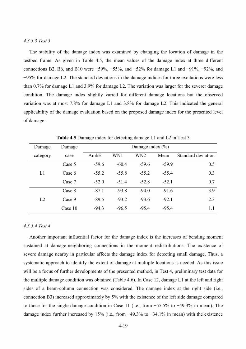
4-19  

4.3.3.3 Test 3

The stability of the damage index was examined by changing the location of damage in the

testbed frame. As given in Table 4.5, the mean values of the damage index at three different

connections B2, B6, and B10 were −59%, −55%, and −52% for damage L1 and −91%, −92%, and

−95% for damage L2. The standard deviations in the damage indices for three excitations were less

than 0.7% for damage L1 and 3.9% for damage L2. The variation was larger for the severer damage

condition. The damage index slightly varied for different damage locations but the observed

variation was at most 7.8% for damage L1 and 3.8% for damage L2. This indicated the general

applicability of the damage evaluation based on the proposed damage index for the presented level

of damage.

Table 4.5 Damage index for detecting damage L1 and L2 in Test 3

Damage

category

Damage

case

Damage index (%)

AmbE WN1 WN2 Mean Standard deviation

L1

Case 5 -59.6 -60.4 -59.6 -59.9 0.5

Case 6 -55.2 -55.8 -55.2 -55.4 0.3

Case 7 -52.0 -51.4 -52.8 -52.1 0.7

L2

Case 8 -87.1 -93.8 -94.0 -91.6 3.9

Case 9 -89.5 -93.2 -93.6 -92.1 2.3

Case 10 -94.3 -96.5 -95.4 -95.4 1.1

4.3.3.4 Test 4

Another important influential factor for the damage index is the increases of bending moment

sustained at damage-neighboring connections in the moment redistributions. The existence of

severe damage nearby in particular affects the damage index for detecting small damage. Thus, a

systematic approach to identify the extent of damage at multiple locations is needed. As this issue

will be a focus of further developments of the presented method, in Test 4, preliminary test data for

the multiple damage condition was obtained (Table 4.6). In Case 12, damage L1 at the left and right

sides of a beam-column connection was considered. The damage index at the right side (i.e.,

connection B3) increased approximately by 5% with the existence of the left side damage compared

to those for the single damage condition in Case 11 (i.e., from −55.5% to −49.3% in mean). The

damage index further increased by 15% (i.e., from −49.3% to −34.1% in mean) with the existence

 

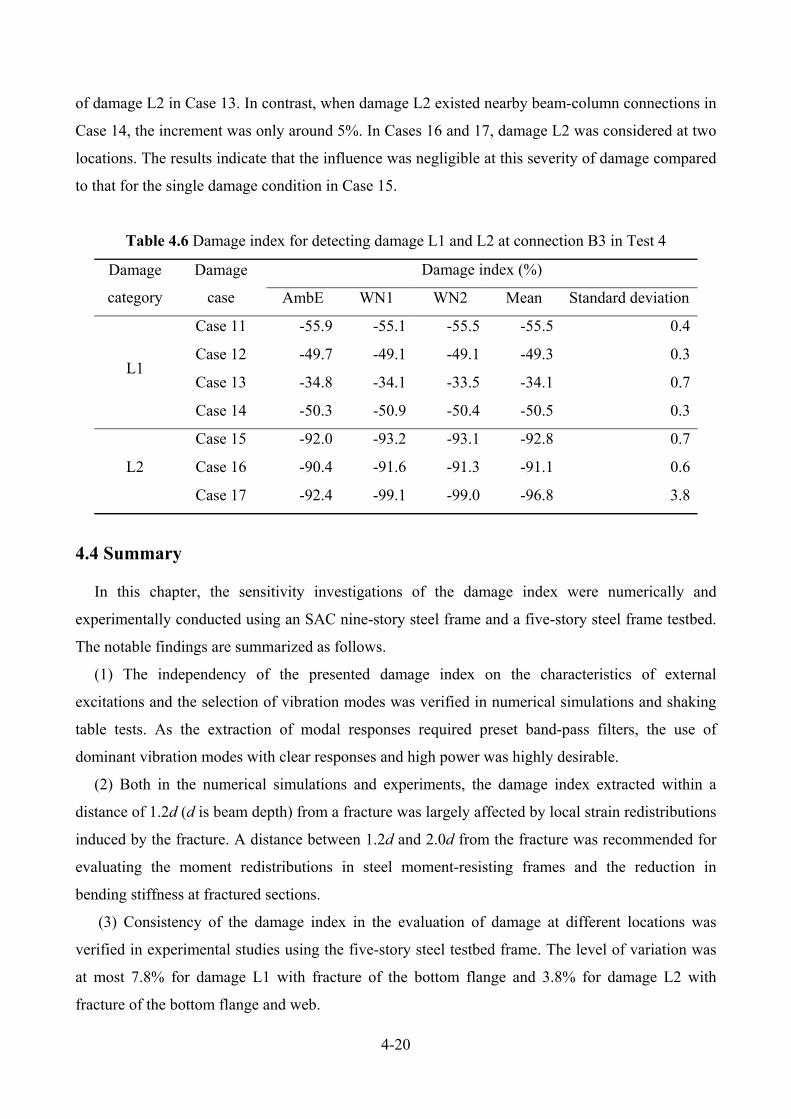
4-20  

of damage L2 in Case 13. In contrast, when damage L2 existed nearby beam-column connections in

Case 14, the increment was only around 5%. In Cases 16 and 17, damage L2 was considered at two

locations. The results indicate that the influence was negligible at this severity of damage compared

to that for the single damage condition in Case 15.

Table 4.6 Damage index for detecting damage L1 and L2 at connection B3 in Test 4

Damage

category

Damage

case

Damage index (%)

AmbE WN1 WN2 Mean Standard deviation

L1

Case 11 -55.9 -55.1 -55.5 -55.5 0.4

Case 12 -49.7 -49.1 -49.1 -49.3 0.3

Case 13 -34.8 -34.1 -33.5 -34.1 0.7

Case 14 -50.3 -50.9 -50.4 -50.5 0.3

L2

Case 15 -92.0 -93.2 -93.1 -92.8 0.7

Case 16 -90.4 -91.6 -91.3 -91.1 0.6

Case 17 -92.4 -99.1 -99.0 -96.8 3.8

4.4 Summary

In this chapter, the sensitivity investigations of the damage index were numerically and

experimentally conducted using an SAC nine-story steel frame and a five-story steel frame testbed.

The notable findings are summarized as follows.

(1) The independency of the presented damage index on the characteristics of external

excitations and the selection of vibration modes was verified in numerical simulations and shaking

table tests. As the extraction of modal responses required preset band-pass filters, the use of

dominant vibration modes with clear responses and high power was highly desirable.

(2) Both in the numerical simulations and experiments, the damage index extracted within a

distance of 1.2d (d is beam depth) from a fracture was largely affected by local strain redistributions

induced by the fracture. A distance between 1.2d and 2.0d from the fracture was recommended for

evaluating the moment redistributions in steel moment-resisting frames and the reduction in

bending stiffness at fractured sections.

(3) Consistency of the damage index in the evaluation of damage at different locations was

verified in experimental studies using the five-story steel testbed frame. The level of variation was

at most 7.8% for damage L1 with fracture of the bottom flange and 3.8% for damage L2 with

fracture of the bottom flange and web.

 

4-21  

(4) The increases of the damage index at damage-neighboring connections were verified using a

preliminary study considering multiple damage condition. The interaction between neighboring

damage at the same beam-column connections was much larger than at different connections. The

explicit effects will be further studied for the damage quantification of multiple beam fractures.

REFERENCES

[1] FEMA-355C. (2000). State of the art report on systems performance of steel moment frames

subject to earthquake ground shaking.

[2] MSC Software Corporation. (2015). http://www.mscsoftware.com/product/marc.

[3] Ohtori Y, Christenson RE, Spencer BF, Dyke SJ. (2004). Benchmark control problems for

seismically excited nonlinear buildings. Journal of Engineering Mechanics, 130(4): 366-385.

 

4-22  

 

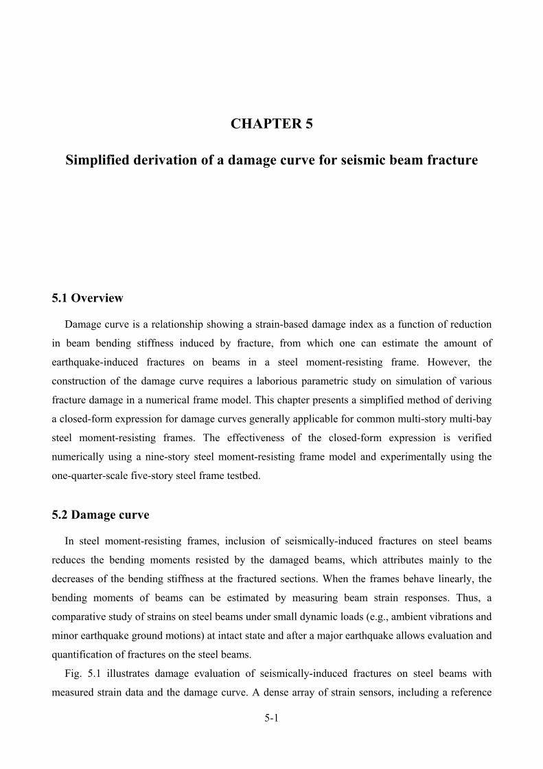
5-1  

CHAPTER 5

Simplified derivation of a damage curve for seismic beam fracture

5.1 Overview

Damage curve is a relationship showing a strain-based damage index as a function of reduction

in beam bending stiffness induced by fracture, from which one can estimate the amount of

earthquake-induced fractures on beams in a steel moment-resisting frame. However, the

construction of the damage curve requires a laborious parametric study on simulation of various

fracture damage in a numerical frame model. This chapter presents a simplified method of deriving

a closed-form expression for damage curves generally applicable for common multi-story multi-bay

steel moment-resisting frames. The effectiveness of the closed-form expression is verified

numerically using a nine-story steel moment-resisting frame model and experimentally using the

one-quarter-scale five-story steel frame testbed.

5.2 Damage curve

In steel moment-resisting frames, inclusion of seismically-induced fractures on steel beams

reduces the bending moments resisted by the damaged beams, which attributes mainly to the

decreases of the bending stiffness at the fractured sections. When the frames behave linearly, the

bending moments of beams can be estimated by measuring beam strain responses. Thus, a

comparative study of strains on steel beams under small dynamic loads (e.g., ambient vibrations and

minor earthquake ground motions) at intact state and after a major earthquake allows evaluation and

quantification of fractures on the steel beams.

Fig. 5.1 illustrates damage evaluation of seismically-induced fractures on steel beams with

measured strain data and the damage curve. A dense array of strain sensors, including a reference

 

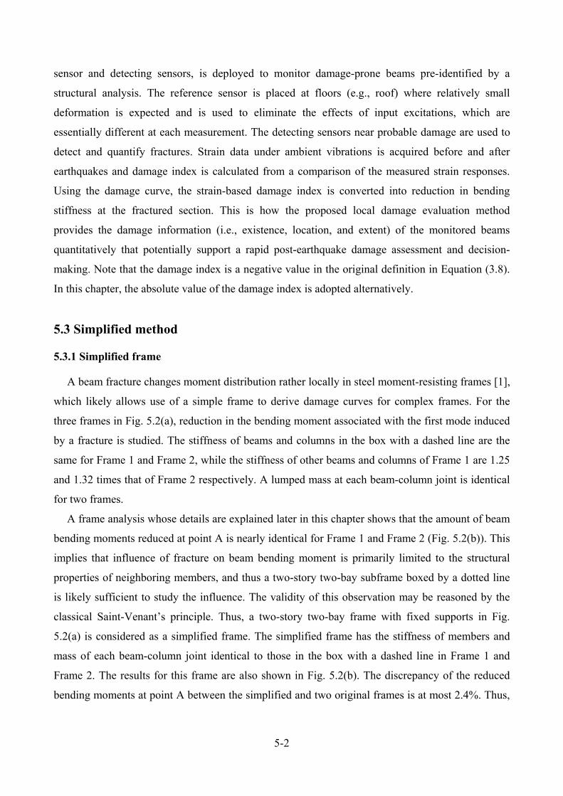
5-2  

sensor and detecting sensors, is deployed to monitor damage-prone beams pre-identified by a

structural analysis. The reference sensor is placed at floors (e.g., roof) where relatively small

deformation is expected and is used to eliminate the effects of input excitations, which are

essentially different at each measurement. The detecting sensors near probable damage are used to

detect and quantify fractures. Strain data under ambient vibrations is acquired before and after

earthquakes and damage index is calculated from a comparison of the measured strain responses.

Using the damage curve, the strain-based damage index is converted into reduction in bending

stiffness at the fractured section. This is how the proposed local damage evaluation method

provides the damage information (i.e., existence, location, and extent) of the monitored beams

quantitatively that potentially support a rapid post-earthquake damage assessment and decision-

making. Note that the damage index is a negative value in the original definition in Equation (3.8).

In this chapter, the absolute value of the damage index is adopted alternatively.

5.3 Simplified method

5.3.1 Simplified frame

A beam fracture changes moment distribution rather locally in steel moment-resisting frames [1],

which likely allows use of a simple frame to derive damage curves for complex frames. For the

three frames in Fig. 5.2(a), reduction in the bending moment associated with the first mode induced

by a fracture is studied. The stiffness of beams and columns in the box with a dashed line are the

same for Frame 1 and Frame 2, while the stiffness of other beams and columns of Frame 1 are 1.25

and 1.32 times that of Frame 2 respectively. A lumped mass at each beam-column joint is identical

for two frames.

A frame analysis whose details are explained later in this chapter shows that the amount of beam

bending moments reduced at point A is nearly identical for Frame 1 and Frame 2 (Fig. 5.2(b)). This

implies that influence of fracture on beam bending moment is primarily limited to the structural

properties of neighboring members, and thus a two-story two-bay subframe boxed by a dotted line

is likely sufficient to study the influence. The validity of this observation may be reasoned by the

classical Saint-Venant’s principle. Thus, a two-story two-bay frame with fixed supports in Fig.

5.2(a) is considered as a simplified frame. The simplified frame has the stiffness of members and

mass of each beam-column joint identical to those in the box with a dashed line in Frame 1 and

Frame 2. The results for this frame are also shown in Fig. 5.2(b). The discrepancy of the reduced

bending moments at point A between the simplified and two original frames is at most 2.4%. Thus,

 

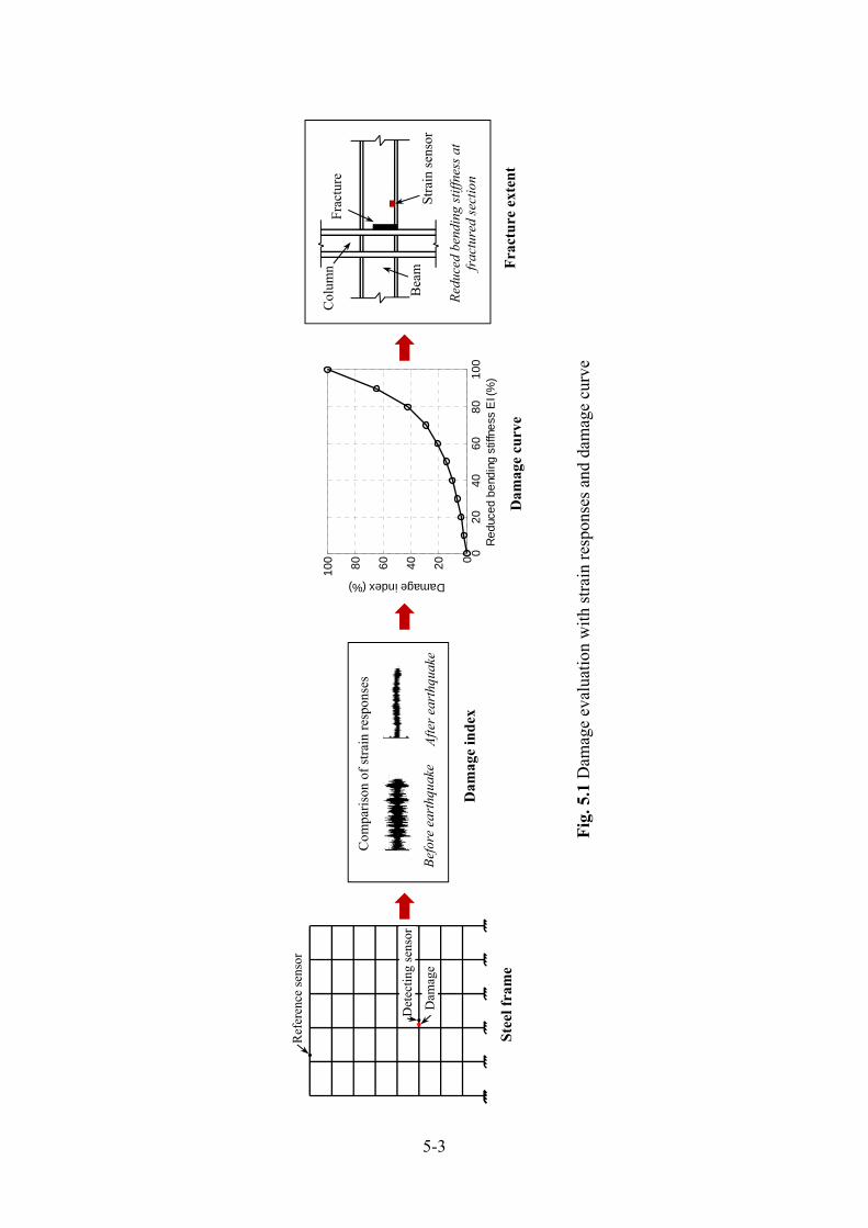
5-3  

Dam

age

ind

ex

Com

pari

son

of s

trai

n re

spon

ses

Bef

ore

eart

hqua

ke

Aft

er e

arth

quak

e

02

04

06

08

01

00

0

20

40

60

80

10

0

Re

duc

ed b

end

ing

stif

fne

ss E

I (%

)

Damage index (%)

Dam

age

curv

e

Col

umn

Fra

ctur

e

Bea

mS

trai

n se

nsor

Fra

ctu

re e

xten

t

Red

uced

ben

ding

sti

ffne

ss a

t fr

actu

red

sect

ion

Dam

age

Det

ecti

ng s

enso

r

Ref

eren

ce s

enso

r

Ste

el f

ram

e

Fig

. 5.1

Dam

age

eval

uati

on w

ith

stra

in r

espo

nses

and

dam

age

curv

e 

 

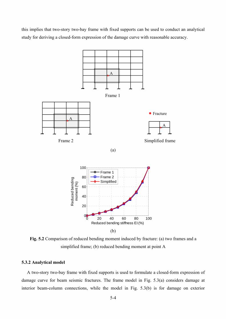
5-4  

this implies that two-story two-bay frame with fixed supports can be used to conduct an analytical

study for deriving a closed-form expression of the damage curve with reasonable accuracy.

(a)

(b)

Fig. 5.2 Comparison of reduced bending moment induced by fracture: (a) two frames and a

simplified frame; (b) reduced bending moment at point A

5.3.2 Analytical model

A two-story two-bay frame with fixed supports is used to formulate a closed-form expression of

damage curve for beam seismic fractures. The frame model in Fig. 5.3(a) considers damage at

interior beam-column connections, while the model in Fig. 5.3(b) is for damage on exterior

0 20 40 60 80 1000

20

40

60

80

100

Reduced bending stiffness EI (%)

Re

du

ced

be

nd

ing

mo

me

nt (

%)

Frame 1Frame 2Simplified

  A

Frame 1

  A

Frame 2 Simplified frame

A

Fracture

 

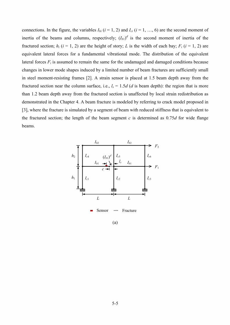
5-5  

connections. In the figure, the variables Ibi (i = 1, 2) and Ici (i = 1, …, 6) are the second moment of

inertia of the beams and columns, respectively; (Ib1)d is the second moment of inertia of the

fractured section; hi (i = 1, 2) are the height of story; L is the width of each bay; Fi (i = 1, 2) are

equivalent lateral forces for a fundamental vibrational mode. The distribution of the equivalent

lateral forces Fi is assumed to remain the same for the undamaged and damaged conditions because

changes in lower mode shapes induced by a limited number of beam fractures are sufficiently small

in steel moment-resisting frames [2]. A strain sensor is placed at 1.5 beam depth away from the

fractured section near the column surface, i.e., ls = 1.5d (d is beam depth): the region that is more

than 1.2 beam depth away from the fractured section is unaffected by local strain redistribution as

demonstrated in the Chapter 4. A beam fracture is modeled by referring to crack model proposed in

[3], where the fracture is simulated by a segment of beam with reduced stiffness that is equivalent to

the fractured section; the length of the beam segment c is determined as 0.75d for wide flange

beams.

(a)

h2

h1

F1

F2

Ic1

Ib1

L

c

(Ib1)d

ls

Ic2 Ic3

Ic4 Ic5 Ic6

Ib1

Ib2 Ib2

L

Sensor Fracture

 

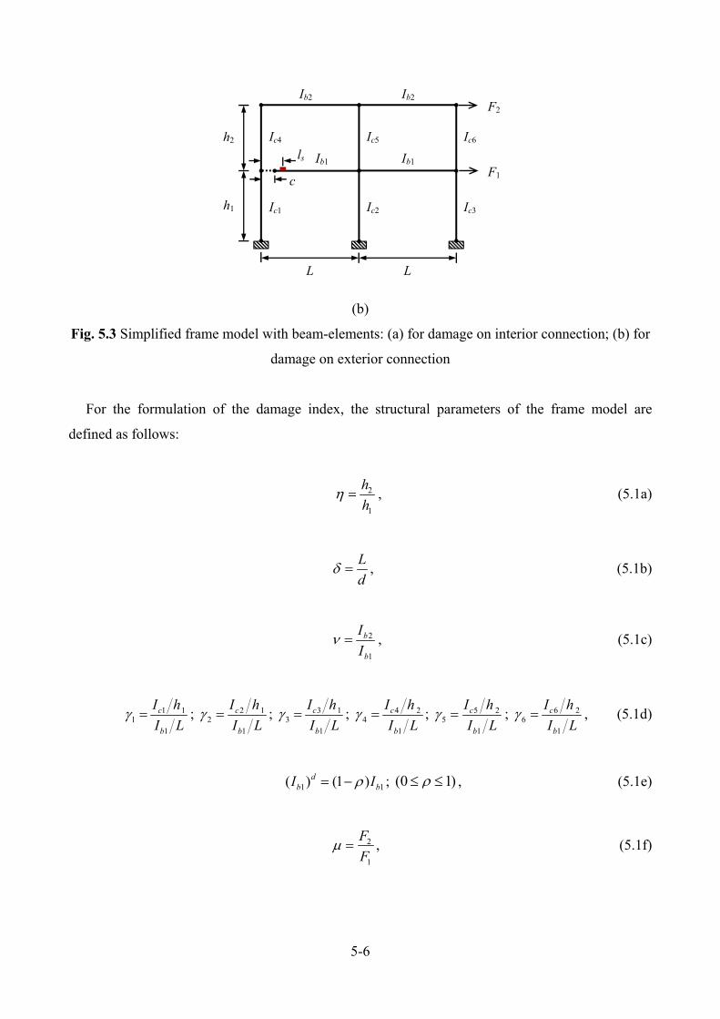
5-6  

(b)

Fig. 5.3 Simplified frame model with beam-elements: (a) for damage on interior connection; (b) for

damage on exterior connection

For the formulation of the damage index, the structural parameters of the frame model are

defined as follows:

2

1

h

h , (5.1a)

L

d , (5.1b)

2

1

b

b

I

I , (5.1c)

1 11

1

c

b

I h

I L ; 2 1

21

c

b

I h

I L ; 3 1

31

c

b

I h

I L ; 4 2

41

c

b

I h

I L ; 5 2

51

c

b

I h

I L ; 6 2

61

c

b

I h

I L , (5.1d)

1 1( ) (1 )db bI I ; (0 1) , (5.1e)

2

1

F

F , (5.1f)

h2

h1

F1

F2

Ic1

Ib1

L

c

ls

Ic2 Ic3

Ic4 Ic5 Ic6

Ib1

Ib2 Ib2

L

 

5-7  

where η is the height ratio between two stories; δ is the span-depth ratio of the fractured beam; ν is

the stiffness ratio between the beams at two floors; γi (i=1, …, 6) are the stiffness ratios of the

column to the beam; ρ is the reduction in the second moment of inertia at the fractured section

(normally expressed as a percentage), i.e., the reduction of bending stiffness at fractured section; μ

is the lateral force ratio between two floors.

The damage index DI, which is equal to the changes of the bending moments at sensor location

between the undamaged and damaged conditions, is a function of reduction in the bending stiffness

at the fractured section ρ as follows:

21 2 3

21 2 3

100%A A A

DIB B B

, (5.2)

where A1, A2, A3, B1, B2, and B3 are coefficients that are a function of structural parameters η, δ, ν, γi

(i=1, …, 6), and μ.

5.3.3 Parametric analysis

The sensitivity of the damage index to the structural parameters η, δ, ν, γi (i=1, …, 6), and μ are

investigated to simplify Equation (5.2). Considering that the structural parameters for common steel

moment-resisting frames vary: 0.5≤ η ≤1; 8≤ δ ≤28; 0.2≤ ν ≤5; 0.5≤ γi ≤2.5 for exterior columns,

0.5≤ γi ≤5 for inner columns; 0.2≤ μ ≤10, two sets of the simplified frames, i.e., Set A for damage

on interior connection; Set B for damage on exterior connection, are considered in parametric

analysis (Table 5.1).

Fig. 5.4 shows the damage curves for all the considered frames. The horizontal axes of the plots

are the reduced bending stiffness at the fractured section and the vertical axes are the damage index

computed with Equation (5.2). In the plots of Subset 1, Subset 3 to Subset 10, Subset 11, and Subset

13 to Subset 20, the damage curves are almost the same for the parameters with different values. In

the plots of Subset 2 and Subset 12, the damage curve changes notably with different span-depth

ratios. The results indicate that the damage curve is primarily affected by the span-depth ratio, and

is insensitive to the other parameters. This is because these parameters that do not affect the damage

curve influence the bending moment distribution at undamaged and damaged conditions in a same

manner, i.e., the damage curve is normalized to these parameters. For the span-depth ratio, as the

beam depth closely relates to the equivalent beam length affected by fracture damage, its influence

 

5-8  

is larger to the bending moment distribution at the damaged conditions than that at the undamaged

conditions, i.e., the damage curve is not normalized to the span-depth ratio.

Table 5.1 Two sets of the simplified frames in parametric analysis

Set A

Default values: η = 1; δ = 10.11; ν = 1; γ1 = γ2 = γ3 = γ4 = γ5 = γ6 =2.13; μ =1.

Subset 1: η = {0.5, 0.6, 0.7, 0.8, 0.9, 1};

Subset 2: δ = {8, 12, 16, 20, 24, 28};

Subset 3: ν = {0.2, 0.6, 1, 3, 5};

Subset 4: γ1 = {0.5, 1, 3, 5};

Subset 5: γ2 = {0.5, 1, 3, 5};

Subset 6: γ3 = {0.5, 1, 3, 5};

Subset 7: γ4 = {0.5, 1, 3, 5};

Subset 8: γ5 = {0.5, 1, 3, 5};

Subset 9: γ6 = {0.5, 1, 3, 5};

Subset 10: μ = {0.2, 0.6, 1, 3, 5, 10}.

Set B

Default values: η = 1; δ = 10.11; ν = 1; γ1 = γ4 =1.61; γ2 = γ3 = γ5 = γ6 =2.13; μ =1.

Subset 11: η = {0.5, 0.6, 0.7, 0.8, 0.9, 1};

Subset 12: δ = {8, 12, 16, 20, 24, 28};

Subset 13: ν = {0.2, 0.6, 1, 3, 5};

Subset 14: γ1 = {0.5, 1, 1.5, 2, 2.5};

Subset 15: γ2 = {0.5, 1, 3, 5};

Subset 16: γ3 = {0.5, 1, 3, 5};

Subset 17: γ4 = {0.5, 1, 1.5, 2, 2.5};

Subset 18: γ5 = {0.5, 1, 3, 5};

Subset 19: γ6 = {0.5, 1, 3, 5};

Subset 20: μ = {0.2, 0.6, 1, 3, 5, 10}.

 

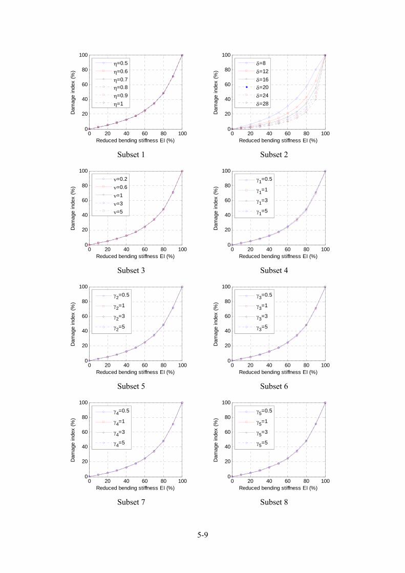
5-9  

Subset 1

Subset 2

Subset 3

Subset 4

Subset 5

Subset 6

Subset 7

Subset 8

0 20 40 60 80 1000

20

40

60

80

100

Reduced bending stiffness EI (%)

Dam

age

inde

x (%

)

=0.5

=0.6

=0.7

=0.8

=0.9

=1

0 20 40 60 80 1000

20

40

60

80

100

Reduced bending stiffness EI (%)

Dam

age

inde

x (%

)

=8

=12

=16

=20

=24

=28

0 20 40 60 80 1000

20

40

60

80

100

Reduced bending stiffness EI (%)

Dam

age

inde

x (%

)

=0.2

=0.6

=1

=3

=5

0 20 40 60 80 1000

20

40

60

80

100

Reduced bending stiffness EI (%)

Dam

age

inde

x (%

)

1=0.5

1=1

1=3

1=5

0 20 40 60 80 1000

20

40

60

80

100

Reduced bending stiffness EI (%)

Dam

age

inde

x (%

)

2=0.5

2=1

2=3

2=5

0 20 40 60 80 1000

20

40

60

80

100

Reduced bending stiffness EI (%)

Dam

age

inde

x (%

)

3=0.5

3=1

3=3

3=5

0 20 40 60 80 1000

20

40

60

80

100

Reduced bending stiffness EI (%)

Dam

age

inde

x (%

)

4=0.5

4=1

4=3

4=5

0 20 40 60 80 1000

20

40

60

80

100

Reduced bending stiffness EI (%)

Dam

age

inde

x (%

)

5=0.5

5=1

5=3

5=5

 

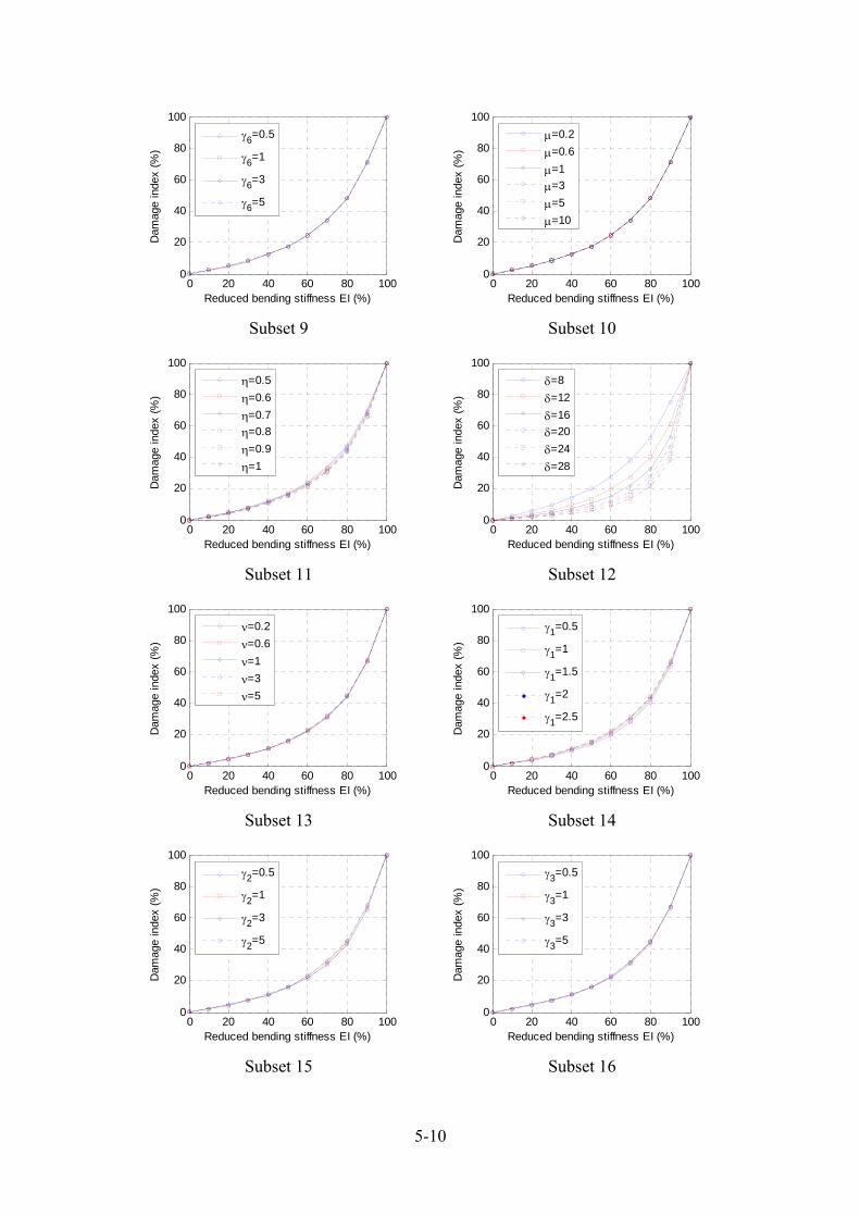
5-10  

Subset 9

Subset 10

Subset 11

Subset 12

Subset 13

Subset 14

Subset 15

Subset 16

0 20 40 60 80 1000

20

40

60

80

100

Reduced bending stiffness EI (%)

Dam

age

inde

x (%

)

6=0.5

6=1

6=3

6=5

0 20 40 60 80 1000

20

40

60

80

100

Reduced bending stiffness EI (%)

Dam

age

inde

x (%

)

=0.2

=0.6

=1

=3

=5

=10

0 20 40 60 80 1000

20

40

60

80

100

Reduced bending stiffness EI (%)

Dam

age

inde

x (%

)

=0.5

=0.6

=0.7

=0.8

=0.9

=1

0 20 40 60 80 1000

20

40

60

80

100

Reduced bending stiffness EI (%)

Dam

age

inde

x (%

)

=8

=12

=16

=20

=24

=28

0 20 40 60 80 1000

20

40

60

80

100

Reduced bending stiffness EI (%)

Dam

age

inde

x (%

)

=0.2

=0.6

=1

=3

=5

0 20 40 60 80 1000

20

40

60

80

100

Reduced bending stiffness EI (%)

Dam

age

inde

x (%

)

1=0.5

1=1

1=1.5

1=2

1=2.5

0 20 40 60 80 1000

20

40

60

80

100

Reduced bending stiffness EI (%)

Dam

age

inde

x (%

)

2=0.5

2=1

2=3

2=5

0 20 40 60 80 1000

20

40

60

80

100

Reduced bending stiffness EI (%)

Dam

age

inde

x (%

)

3=0.5

3=1

3=3

3=5

 

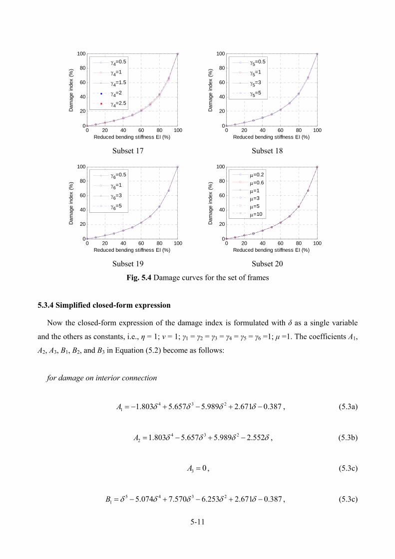
5-11  

Subset 17

Subset 18

Subset 19

Subset 20

Fig. 5.4 Damage curves for the set of frames

5.3.4 Simplified closed-form expression

Now the closed-form expression of the damage index is formulated with δ as a single variable

and the others as constants, i.e., η = 1; ν = 1; γ1 = γ2 = γ3 = γ4 = γ5 = γ6 =1; μ =1. The coefficients A1,

A2, A3, B1, B2, and B3 in Equation (5.2) become as follows:

for damage on interior connection

4 3 21 1.803 5.657 5.989 2.671 0.387A , (5.3a)

4 3 22 1.803 5.657 5.989 2.552A , (5.3b)

3 0A , (5.3c)

5 4 3 21 5.074 7.570 6.253 2.671 0.387B , (5.3c)

0 20 40 60 80 1000

20

40

60

80

100

Reduced bending stiffness EI (%)

Dam

age

inde

x (%

)

4=0.5

4=1

4=1.5

4=2

4=2.5

0 20 40 60 80 1000

20

40

60

80

100

Reduced bending stiffness EI (%)

Dam

age

inde

x (%

)

5=0.5

5=1

5=3

5=5

0 20 40 60 80 1000

20

40

60

80

100

Reduced bending stiffness EI (%)

Dam

age

inde

x (%

)

6=0.5

6=1

6=3

6=5

0 20 40 60 80 1000

20

40

60

80

100

Reduced bending stiffness EI (%)

Dam

age

inde

x (%

)

=0.2

=0.6

=1

=3

=5

=10

 

5-12  

5 4 3 22 2.000 8.345 7.570 6.253 2.552B , (5.3d)

5 43 3.271B , (5.3e)

for damage on exterior connection

4 3 21 1.502 4.659 5.014 2.280 0.328A , (5.3f)

4 3 22 1.502 4.659 5.014 2.161A , (5.3g)

3 0A , (5.3h)

5 4 3 21 4.272 5.608 4.791 2.280 0.328B , (5.3i)

5 4 3 22 2.000 7.042 5.608 4.791 2.161B , (5.3j)

5 43 2.770B , (5.3k)

Fig. 5.5 illustrates the damage curves derived from the simplified expression including numerical

error. When the reduced bending stiffness approaches 100%, the damage index exceeds 100% in the

cases where the span-depth ratio equals 8 and 10 for damage on interior connection and the span-

depth ratio equals 8 for damage on exterior connection. This is because when the reduced bending

stiffness is close to 100%, the values of numerator and denominator of Equation (5.2) are about zero

(Fig. 5.6) and thus bring some numerical error in those three cases. Practically, when the reduced

bending stiffness is more than 90%, i.e., almost complete fracture, the damage index is about 100%.

Hence, the damage index of more than 100% can be reasonably rectified as 100%.

 

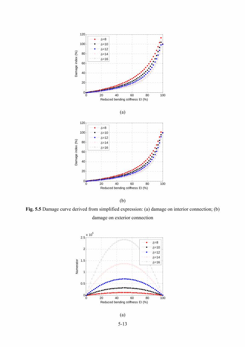
5-13  

(a)

(b)

Fig. 5.5 Damage curve derived from simplified expression: (a) damage on interior connection; (b)

damage on exterior connection

(a)

0 20 40 60 80 1000

20

40

60

80

100

120

Reduced bending stiffness EI (%)

Dam

age

inde

x (%

)

=8

=10

=12

=14

=16

0 20 40 60 80 1000

20

40

60

80

100

120

Reduced bending stiffness EI (%)

Dam

age

inde

x (%

)

=8

=10

=12

=14

=16

0 20 40 60 80 1000

0.5

1

1.5

2

2.5x 10

6

Reduced bending stiffness EI (%)

Num

erat

or

=8

=10

=12

=14

=16

 

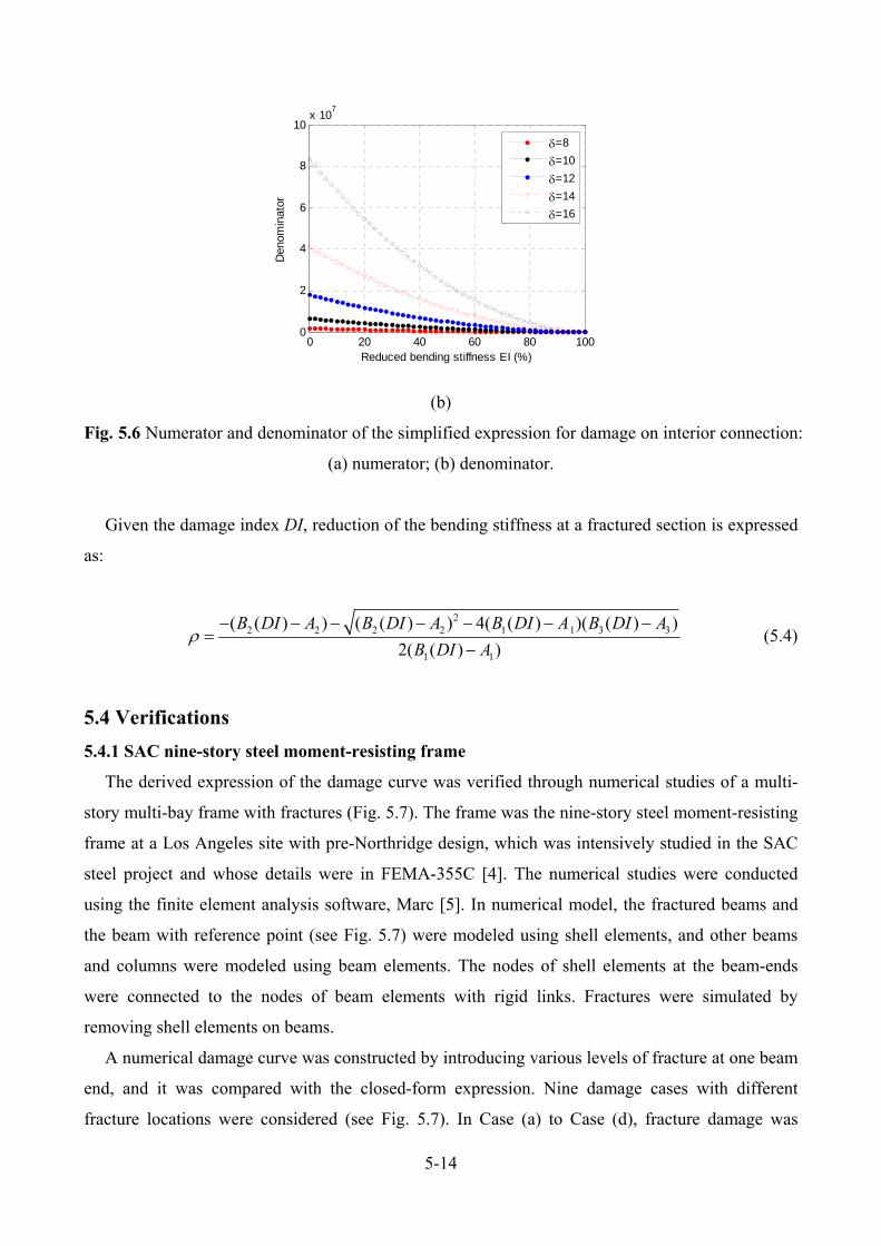
5-14  

(b)

Fig. 5.6 Numerator and denominator of the simplified expression for damage on interior connection:

(a) numerator; (b) denominator.

Given the damage index DI, reduction of the bending stiffness at a fractured section is expressed

as:

22 2 2 2 1 1 3 3

1 1

( ( ) ) ( ( ) ) 4( ( ) )( ( ) )

2( ( ) )

B DI A B DI A B DI A B DI A

B DI A

(5.4)

5.4 Verifications

5.4.1 SAC nine-story steel moment-resisting frame

The derived expression of the damage curve was verified through numerical studies of a multi-

story multi-bay frame with fractures (Fig. 5.7). The frame was the nine-story steel moment-resisting

frame at a Los Angeles site with pre-Northridge design, which was intensively studied in the SAC

steel project and whose details were in FEMA-355C [4]. The numerical studies were conducted

using the finite element analysis software, Marc [5]. In numerical model, the fractured beams and

the beam with reference point (see Fig. 5.7) were modeled using shell elements, and other beams

and columns were modeled using beam elements. The nodes of shell elements at the beam-ends

were connected to the nodes of beam elements with rigid links. Fractures were simulated by

removing shell elements on beams.

A numerical damage curve was constructed by introducing various levels of fracture at one beam

end, and it was compared with the closed-form expression. Nine damage cases with different

fracture locations were considered (see Fig. 5.7). In Case (a) to Case (d), fracture damage was

0 20 40 60 80 1000

2

4

6

8

10x 10

7

Reduced bending stiffness EI (%)

Den

omin

ator

=8

=10

=12

=14

=16

 

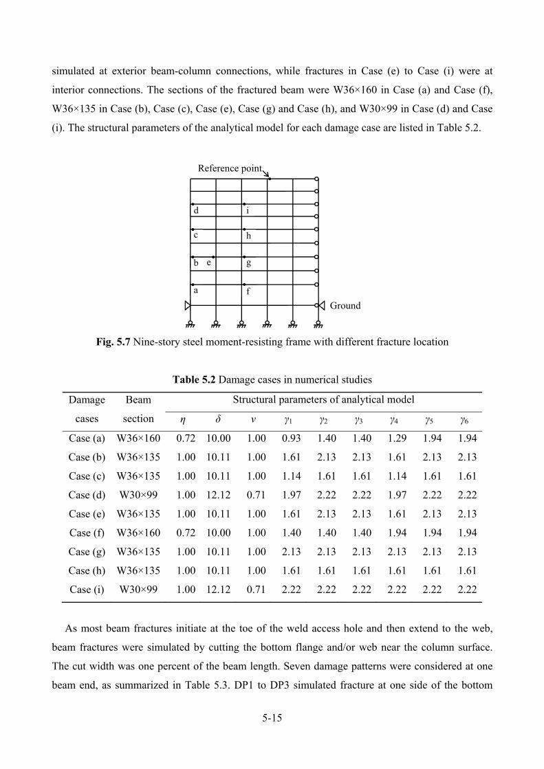
5-15  

simulated at exterior beam-column connections, while fractures in Case (e) to Case (i) were at

interior connections. The sections of the fractured beam were W36×160 in Case (a) and Case (f),

W36×135 in Case (b), Case (c), Case (e), Case (g) and Case (h), and W30×99 in Case (d) and Case

(i). The structural parameters of the analytical model for each damage case are listed in Table 5.2.

Fig. 5.7 Nine-story steel moment-resisting frame with different fracture location

Table 5.2 Damage cases in numerical studies

Damage

cases

Beam

section

Structural parameters of analytical model

η δ ν γ1 γ2 γ3 γ4 γ5 γ6

Case (a) W36×160 0.72 10.00 1.00 0.93 1.40 1.40 1.29 1.94 1.94

Case (b) W36×135 1.00 10.11 1.00 1.61 2.13 2.13 1.61 2.13 2.13

Case (c) W36×135 1.00 10.11 1.00 1.14 1.61 1.61 1.14 1.61 1.61

Case (d) W30×99 1.00 12.12 0.71 1.97 2.22 2.22 1.97 2.22 2.22

Case (e) W36×135 1.00 10.11 1.00 1.61 2.13 2.13 1.61 2.13 2.13

Case (f) W36×160 0.72 10.00 1.00 1.40 1.40 1.40 1.94 1.94 1.94

Case (g) W36×135 1.00 10.11 1.00 2.13 2.13 2.13 2.13 2.13 2.13

Case (h) W36×135 1.00 10.11 1.00 1.61 1.61 1.61 1.61 1.61 1.61

Case (i) W30×99 1.00 12.12 0.71 2.22 2.22 2.22 2.22 2.22 2.22

As most beam fractures initiate at the toe of the weld access hole and then extend to the web,

beam fractures were simulated by cutting the bottom flange and/or web near the column surface.

The cut width was one percent of the beam length. Seven damage patterns were considered at one

beam end, as summarized in Table 5.3. DP1 to DP3 simulated fracture at one side of the bottom

Ground

a f

b e g

c h

d i

Reference point

 

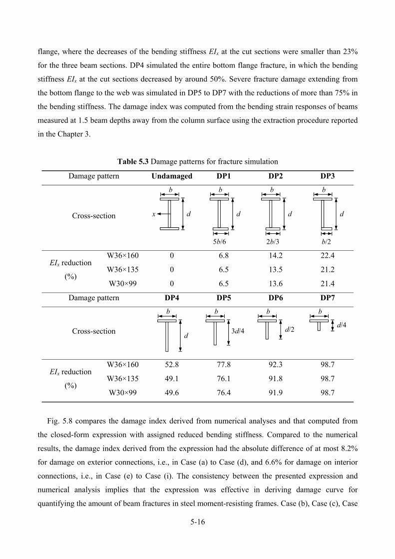
5-16  

flange, where the decreases of the bending stiffness EIx at the cut sections were smaller than 23%

for the three beam sections. DP4 simulated the entire bottom flange fracture, in which the bending

stiffness EIx at the cut sections decreased by around 50%. Severe fracture damage extending from

the bottom flange to the web was simulated in DP5 to DP7 with the reductions of more than 75% in

the bending stiffness. The damage index was computed from the bending strain responses of beams

measured at 1.5 beam depths away from the column surface using the extraction procedure reported

in the Chapter 3.

Table 5.3 Damage patterns for fracture simulation

Damage pattern Undamaged DP1 DP2 DP3

Cross-section

EIx reduction

(%)

W36×160 0 6.8 14.2 22.4

W36×135 0 6.5 13.5 21.2

W30×99 0 6.5 13.6 21.4

Damage pattern DP4 DP5 DP6 DP7

Cross-section

EIx reduction

(%)

W36×160 52.8 77.8 92.3 98.7

W36×135 49.1 76.1 91.8 98.7

W30×99 49.6 76.4 91.9 98.7

Fig. 5.8 compares the damage index derived from numerical analyses and that computed from

the closed-form expression with assigned reduced bending stiffness. Compared to the numerical

results, the damage index derived from the expression had the absolute difference of at most 8.2%

for damage on exterior connections, i.e., in Case (a) to Case (d), and 6.6% for damage on interior

connections, i.e., in Case (e) to Case (i). The consistency between the presented expression and

numerical analysis implies that the expression was effective in deriving damage curve for

quantifying the amount of beam fractures in steel moment-resisting frames. Case (b), Case (c), Case

b

dx

b

d

5b/6

b

d

2b/3

b

d

b/2

b

d

b

3d/4  

b

d/2

b

d/4

 

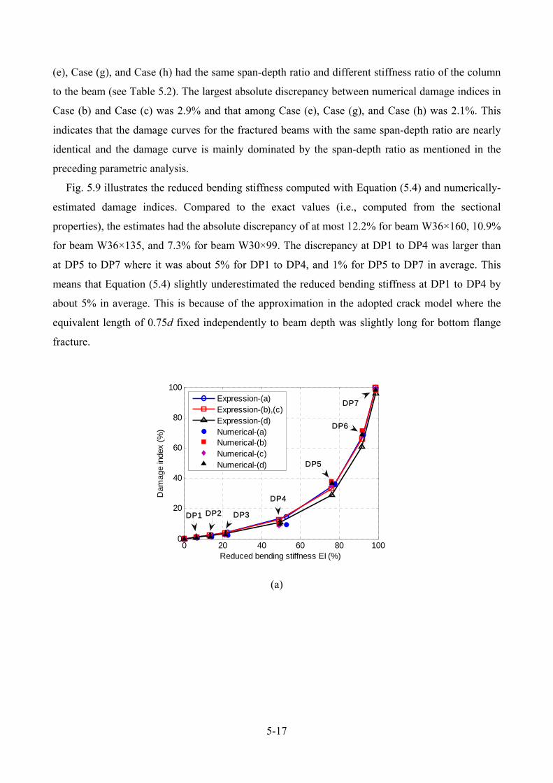
5-17  

(e), Case (g), and Case (h) had the same span-depth ratio and different stiffness ratio of the column

to the beam (see Table 5.2). The largest absolute discrepancy between numerical damage indices in

Case (b) and Case (c) was 2.9% and that among Case (e), Case (g), and Case (h) was 2.1%. This

indicates that the damage curves for the fractured beams with the same span-depth ratio are nearly

identical and the damage curve is mainly dominated by the span-depth ratio as mentioned in the

preceding parametric analysis.

Fig. 5.9 illustrates the reduced bending stiffness computed with Equation (5.4) and numerically-

estimated damage indices. Compared to the exact values (i.e., computed from the sectional

properties), the estimates had the absolute discrepancy of at most 12.2% for beam W36×160, 10.9%

for beam W36×135, and 7.3% for beam W30×99. The discrepancy at DP1 to DP4 was larger than

at DP5 to DP7 where it was about 5% for DP1 to DP4, and 1% for DP5 to DP7 in average. This

means that Equation (5.4) slightly underestimated the reduced bending stiffness at DP1 to DP4 by

about 5% in average. This is because of the approximation in the adopted crack model where the

equivalent length of 0.75d fixed independently to beam depth was slightly long for bottom flange

fracture.

(a)

0 20 40 60 80 1000

20

40

60

80

100

Reduced bending stiffness EI (%)

Dam

age

inde

x (%

)

Expression-(a)Expression-(b),(c)Expression-(d)Numerical-(a)Numerical-(b)Numerical-(c)Numerical-(d)

DP1 DP3

DP4

DP5

DP6

DP7

DP2

 

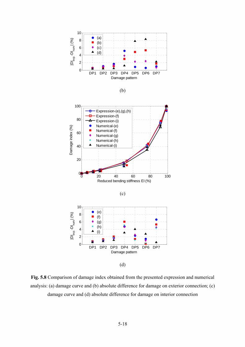
5-18  

(b)

(c)

(d)

Fig. 5.8 Comparison of damage index obtained from the presented expression and numerical

analysis: (a) damage curve and (b) absolute difference for damage on exterior connection; (c)

damage curve and (d) absolute difference for damage on interior connection

DP1 DP2 DP3 DP4 DP5 DP6 DP70

2

4

6

8

10

Damage pattern

|DI ex

p.-D

I num

.| (%

)

(a)(b)(c)(d)

0 20 40 60 80 1000

20

40

60

80

100

Reduced bending stiffness EI (%)

Dam

age

inde

x (%

)

Expression-(e),(g),(h)Expression-(f)Expression-(i)Numerical-(e)Numerical-(f)Numerical-(g)Numerical-(h)Numerical-(i)

DP1 DP2 DP3 DP4 DP5 DP6 DP70

2

4

6

8

10

Damage pattern

|DI ex

p.-D

I num

.| (%

)

(e)(f)(g)(h)(i)

 

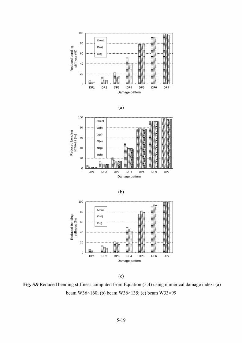
5-19  

(a)

(b)

(c)

Fig. 5.9 Reduced bending stiffness computed from Equation (5.4) using numerical damage index: (a)

beam W36×160; (b) beam W36×135; (c) beam W33×99

0

20

40

60

80

100

DP1 DP2 DP3 DP4 DP5 DP6 DP7

Red

uced

ben

ding

st

iffne

ss (

%)

Damage pattern

real

(a)

(f)

0

20

40

60

80

100

DP1 DP2 DP3 DP4 DP5 DP6 DP7

Red

uced

ben

ding

st

iffne

ss (

%)

Damage pattern

real

(b)

(c)

(e)

(g)

(h)

0

20

40

60

80

100

DP1 DP2 DP3 DP4 DP5 DP6 DP7

Red

uced

ben

ding

st

iffne

ss (

%)

Damage pattern

real

(d)

(i)

 

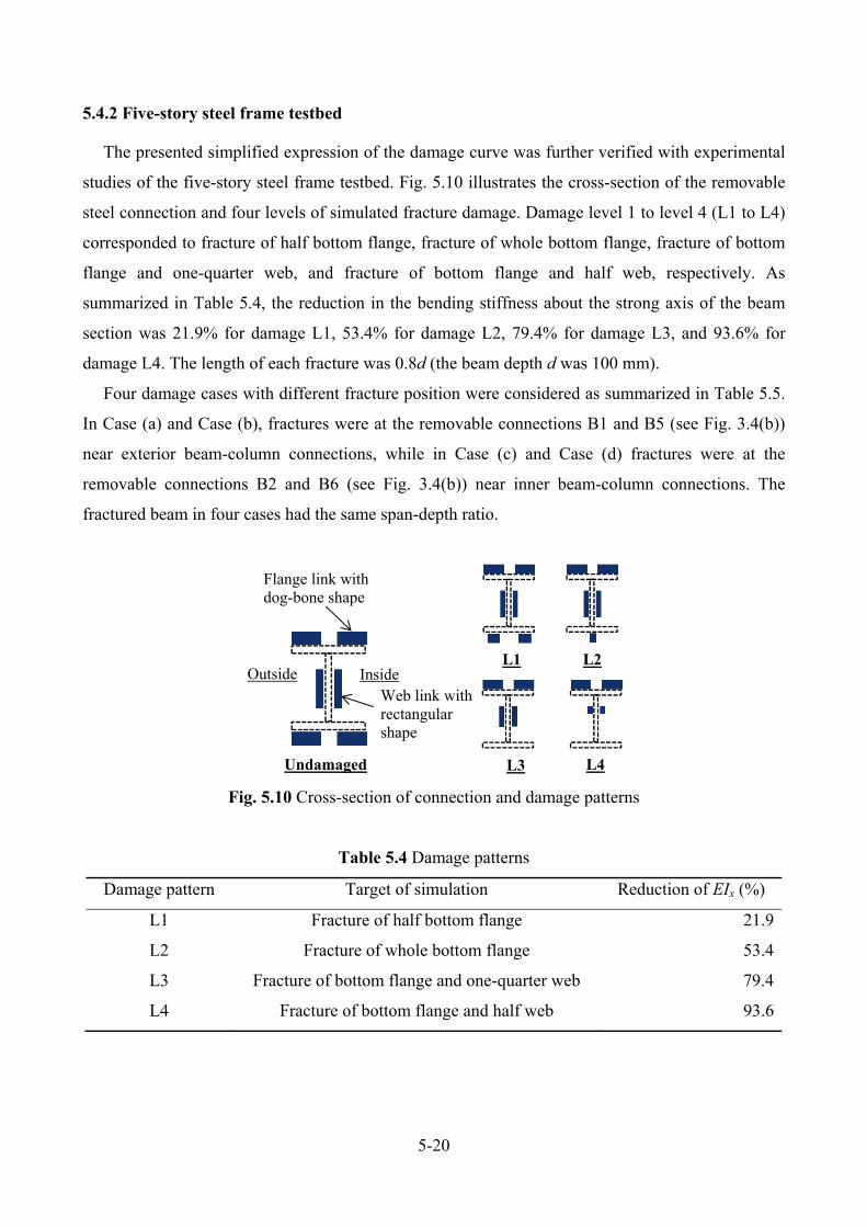
5-20  

5.4.2 Five-story steel frame testbed

The presented simplified expression of the damage curve was further verified with experimental

studies of the five-story steel frame testbed. Fig. 5.10 illustrates the cross-section of the removable

steel connection and four levels of simulated fracture damage. Damage level 1 to level 4 (L1 to L4)

corresponded to fracture of half bottom flange, fracture of whole bottom flange, fracture of bottom

flange and one-quarter web, and fracture of bottom flange and half web, respectively. As

summarized in Table 5.4, the reduction in the bending stiffness about the strong axis of the beam

section was 21.9% for damage L1, 53.4% for damage L2, 79.4% for damage L3, and 93.6% for

damage L4. The length of each fracture was 0.8d (the beam depth d was 100 mm).

Four damage cases with different fracture position were considered as summarized in Table 5.5.

In Case (a) and Case (b), fractures were at the removable connections B1 and B5 (see Fig. 3.4(b))

near exterior beam-column connections, while in Case (c) and Case (d) fractures were at the

removable connections B2 and B6 (see Fig. 3.4(b)) near inner beam-column connections. The

fractured beam in four cases had the same span-depth ratio.

Fig. 5.10 Cross-section of connection and damage patterns

Table 5.4 Damage patterns

Damage pattern Target of simulation Reduction of EIx (%)

L1 Fracture of half bottom flange 21.9

L2 Fracture of whole bottom flange 53.4

L3 Fracture of bottom flange and one-quarter web 79.4

L4 Fracture of bottom flange and half web 93.6

Flange link with dog-bone shape

Web link with rectangular shape

Outside InsideL1 L2

L3 L4Undamaged

 

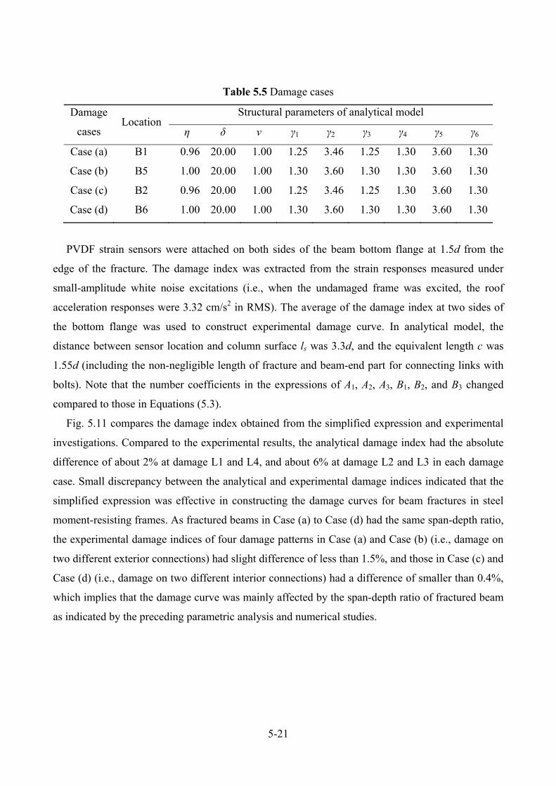
5-21  

Table 5.5 Damage cases

Damage

cases Location

Structural parameters of analytical model

η δ ν γ1 γ2 γ3 γ4 γ5 γ6

Case (a) B1 0.96 20.00 1.00 1.25 3.46 1.25 1.30 3.60 1.30

Case (b) B5 1.00 20.00 1.00 1.30 3.60 1.30 1.30 3.60 1.30

Case (c) B2 0.96 20.00 1.00 1.25 3.46 1.25 1.30 3.60 1.30

Case (d) B6 1.00 20.00 1.00 1.30 3.60 1.30 1.30 3.60 1.30

PVDF strain sensors were attached on both sides of the beam bottom flange at 1.5d from the

edge of the fracture. The damage index was extracted from the strain responses measured under

small-amplitude white noise excitations (i.e., when the undamaged frame was excited, the roof

acceleration responses were 3.32 cm/s2 in RMS). The average of the damage index at two sides of

the bottom flange was used to construct experimental damage curve. In analytical model, the

distance between sensor location and column surface ls was 3.3d, and the equivalent length c was

1.55d (including the non-negligible length of fracture and beam-end part for connecting links with

bolts). Note that the number coefficients in the expressions of A1, A2, A3, B1, B2, and B3 changed

compared to those in Equations (5.3).

Fig. 5.11 compares the damage index obtained from the simplified expression and experimental

investigations. Compared to the experimental results, the analytical damage index had the absolute

difference of about 2% at damage L1 and L4, and about 6% at damage L2 and L3 in each damage

case. Small discrepancy between the analytical and experimental damage indices indicated that the

simplified expression was effective in constructing the damage curves for beam fractures in steel

moment-resisting frames. As fractured beams in Case (a) to Case (d) had the same span-depth ratio,

the experimental damage indices of four damage patterns in Case (a) and Case (b) (i.e., damage on

two different exterior connections) had slight difference of less than 1.5%, and those in Case (c) and

Case (d) (i.e., damage on two different interior connections) had a difference of smaller than 0.4%,

which implies that the damage curve was mainly affected by the span-depth ratio of fractured beam

as indicated by the preceding parametric analysis and numerical studies.

 

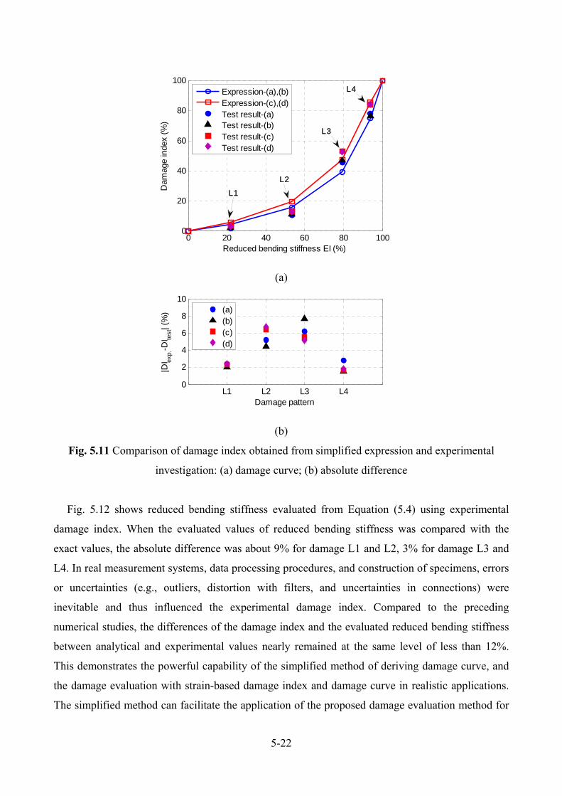
5-22  

(a)

(b)

Fig. 5.11 Comparison of damage index obtained from simplified expression and experimental

investigation: (a) damage curve; (b) absolute difference

Fig. 5.12 shows reduced bending stiffness evaluated from Equation (5.4) using experimental

damage index. When the evaluated values of reduced bending stiffness was compared with the

exact values, the absolute difference was about 9% for damage L1 and L2, 3% for damage L3 and

L4. In real measurement systems, data processing procedures, and construction of specimens, errors

or uncertainties (e.g., outliers, distortion with filters, and uncertainties in connections) were

inevitable and thus influenced the experimental damage index. Compared to the preceding

numerical studies, the differences of the damage index and the evaluated reduced bending stiffness

between analytical and experimental values nearly remained at the same level of less than 12%.

This demonstrates the powerful capability of the simplified method of deriving damage curve, and

the damage evaluation with strain-based damage index and damage curve in realistic applications.

The simplified method can facilitate the application of the proposed damage evaluation method for

0 20 40 60 80 1000

20

40

60

80

100

Reduced bending stiffness EI (%)

Dam

age

inde

x (%

)

Expression-(a),(b)Expression-(c),(d)Test result-(a)Test result-(b)Test result-(c)Test result-(d)

L1

L2

L3

L4

L1 L2 L3 L40

2

4

6

8

10

Damage pattern

|DI ex

p.-D

I test

| (%

)

(a)(b)(c)(d)

 

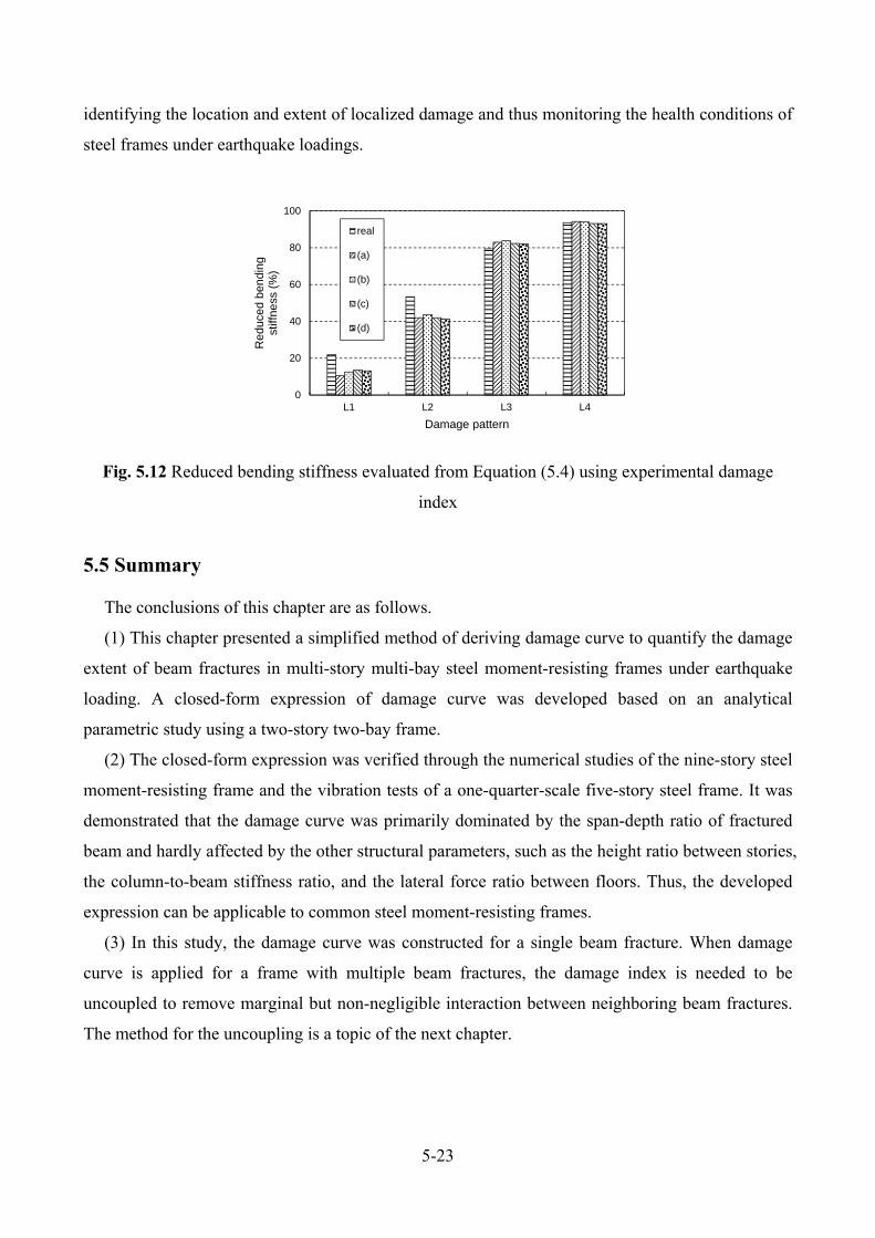
5-23  

identifying the location and extent of localized damage and thus monitoring the health conditions of

steel frames under earthquake loadings.

Fig. 5.12 Reduced bending stiffness evaluated from Equation (5.4) using experimental damage

index

5.5 Summary

The conclusions of this chapter are as follows.

(1) This chapter presented a simplified method of deriving damage curve to quantify the damage

extent of beam fractures in multi-story multi-bay steel moment-resisting frames under earthquake

loading. A closed-form expression of damage curve was developed based on an analytical

parametric study using a two-story two-bay frame.

(2) The closed-form expression was verified through the numerical studies of the nine-story steel

moment-resisting frame and the vibration tests of a one-quarter-scale five-story steel frame. It was

demonstrated that the damage curve was primarily dominated by the span-depth ratio of fractured

beam and hardly affected by the other structural parameters, such as the height ratio between stories,

the column-to-beam stiffness ratio, and the lateral force ratio between floors. Thus, the developed

expression can be applicable to common steel moment-resisting frames.

(3) In this study, the damage curve was constructed for a single beam fracture. When damage

curve is applied for a frame with multiple beam fractures, the damage index is needed to be

uncoupled to remove marginal but non-negligible interaction between neighboring beam fractures.

The method for the uncoupling is a topic of the next chapter.

0

20

40

60

80

100

L1 L2 L3 L4

Red

uced

ben

ding

st

iffne

ss (

%)

Damage pattern

real

(a)

(b)

(c)

(d)

 

5-24  

REFERENCES

[1] Nakashima M., Minami T., and Mitani I. (2000). Moment Redistribution Caused by Beam

Fracture in Steel Moment Frames. J. Struct. Eng., 126(1): 137–144.

[2] Ji X., Fenves G., Kajiwara K., and Nakashima M. (2011). Seismic damage detection of a full-

scale shaking table test structure. Journal of Structural Engineering, 137(6): 14-21.

[3] Sinha J. K., Friswell M. I., and Edwards S. (2002). Simplified models for the location of

cracks in beam structures using measured vibration data. Journal of Sound and Vibration,

251(1):13-38.

[4] FEMA-355C. (2000). State of the art report on systems performance of steel moment frames

subject to earthquake ground shaking.

[5] MSC Software Corporation. (2015). http://www.mscsoftware.com/product/marc.

 

 

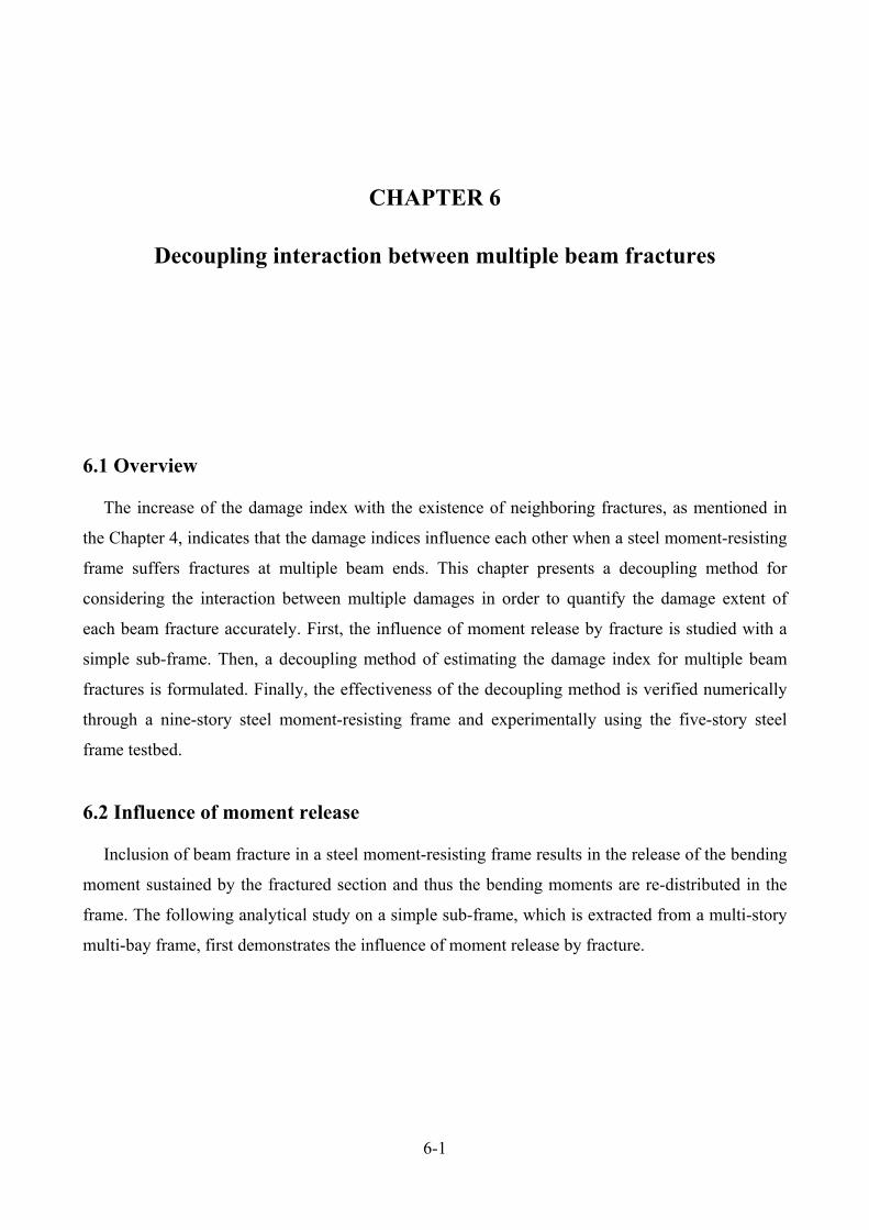
6-1  

CHAPTER 6

Decoupling interaction between multiple beam fractures

 

 

 

 

6.1 Overview

The increase of the damage index with the existence of neighboring fractures, as mentioned in

the Chapter 4, indicates that the damage indices influence each other when a steel moment-resisting

frame suffers fractures at multiple beam ends. This chapter presents a decoupling method for

considering the interaction between multiple damages in order to quantify the damage extent of

each beam fracture accurately. First, the influence of moment release by fracture is studied with a

simple sub-frame. Then, a decoupling method of estimating the damage index for multiple beam

fractures is formulated. Finally, the effectiveness of the decoupling method is verified numerically

through a nine-story steel moment-resisting frame and experimentally using the five-story steel

frame testbed.

6.2 Influence of moment release

Inclusion of beam fracture in a steel moment-resisting frame results in the release of the bending

moment sustained by the fractured section and thus the bending moments are re-distributed in the

frame. The following analytical study on a simple sub-frame, which is extracted from a multi-story

multi-bay frame, first demonstrates the influence of moment release by fracture.

 

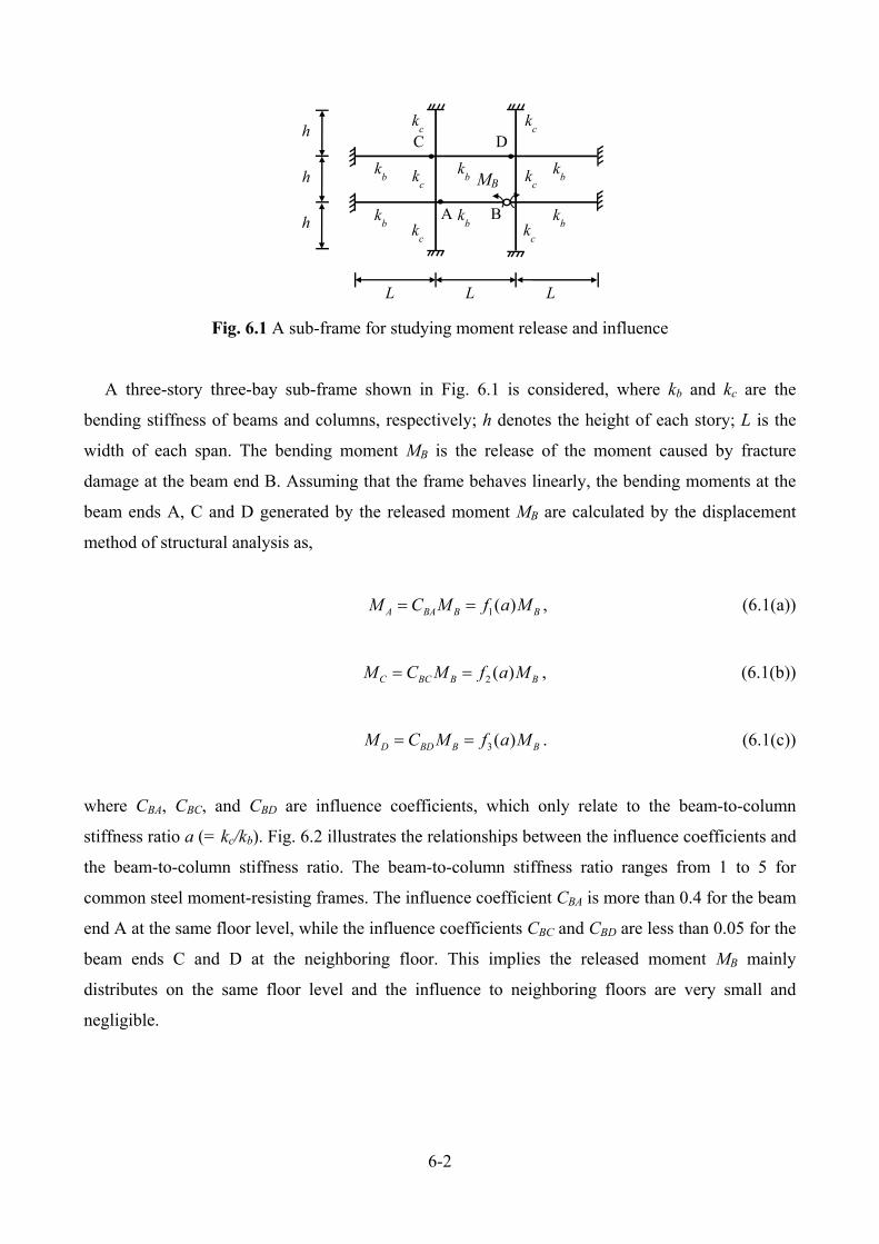
6-2  

Fig. 6.1 A sub-frame for studying moment release and influence

A three-story three-bay sub-frame shown in Fig. 6.1 is considered, where kb and kc are the

bending stiffness of beams and columns, respectively; h denotes the height of each story; L is the

width of each span. The bending moment MB is the release of the moment caused by fracture

damage at the beam end B. Assuming that the frame behaves linearly, the bending moments at the

beam ends A, C and D generated by the released moment MB are calculated by the displacement

method of structural analysis as,

1( )A BA B BM C M f a M , (6.1(a))

2 ( )C BC B BM C M f a M , (6.1(b))

3( )D BD B BM C M f a M . (6.1(c))

where CBA, CBC, and CBD are influence coefficients, which only relate to the beam-to-column

stiffness ratio a (= kc/kb). Fig. 6.2 illustrates the relationships between the influence coefficients and

the beam-to-column stiffness ratio. The beam-to-column stiffness ratio ranges from 1 to 5 for

common steel moment-resisting frames. The influence coefficient CBA is more than 0.4 for the beam

end A at the same floor level, while the influence coefficients CBC and CBD are less than 0.05 for the

beam ends C and D at the neighboring floor. This implies the released moment MB mainly

distributes on the same floor level and the influence to neighboring floors are very small and

negligible.

kc

kc

kc

MB

A B

C D

kc

kc

kc

kb

kb

kb

kb

kb

kb

L L L

h

h

h

 

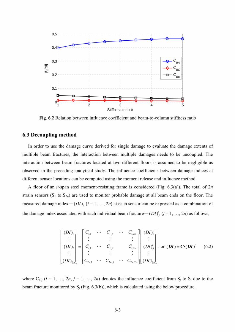
6-3  

Fig. 6.2 Relation between influence coefficient and beam-to-column stiffness ratio

6.3 Decoupling method

In order to use the damage curve derived for single damage to evaluate the damage extents of

multiple beam fractures, the interaction between multiple damages needs to be uncoupled. The

interaction between beam fractures located at two different floors is assumed to be negligible as

observed in the preceding analytical study. The influence coefficients between damage indices at

different sensor locations can be computed using the moment release and influence method.

A floor of an n-span steel moment-resisting frame is considered (Fig. 6.3(a)). The total of 2n

strain sensors (S1 to S2n) are used to monitor probable damage at all beam ends on the floor. The

measured damage index― ( )iDI (i = 1, …, 2n) at each sensor can be expressed as a combination of

the damage index associated with each individual beam fracture― ( ) jDI (j = 1, …, 2n) as follows,

1,1 1, 1,21 1

,1 , ,2

2 ,1 2 , 2 ,22 2

( ) ( )

( ) ( )

( ) ( )

j n

i i j i ni j

n n j n nn n

C C CDI DI

C C CDI DI

C C CDI DI

, or ( ) ( )DI C DI (6.2)

where Ci, j (i = 1, …, 2n, j = 1, …, 2n) denotes the influence coefficient from Sj to Si due to the

beam fracture monitored by Sj (Fig. 6.3(b)), which is calculated using the below procedure.

1 2 3 4 50

0.1

0.2

0.3

0.4

0.5

Stiffness ratio a

|f i (a

)|

CBA

CBC

CBD

 

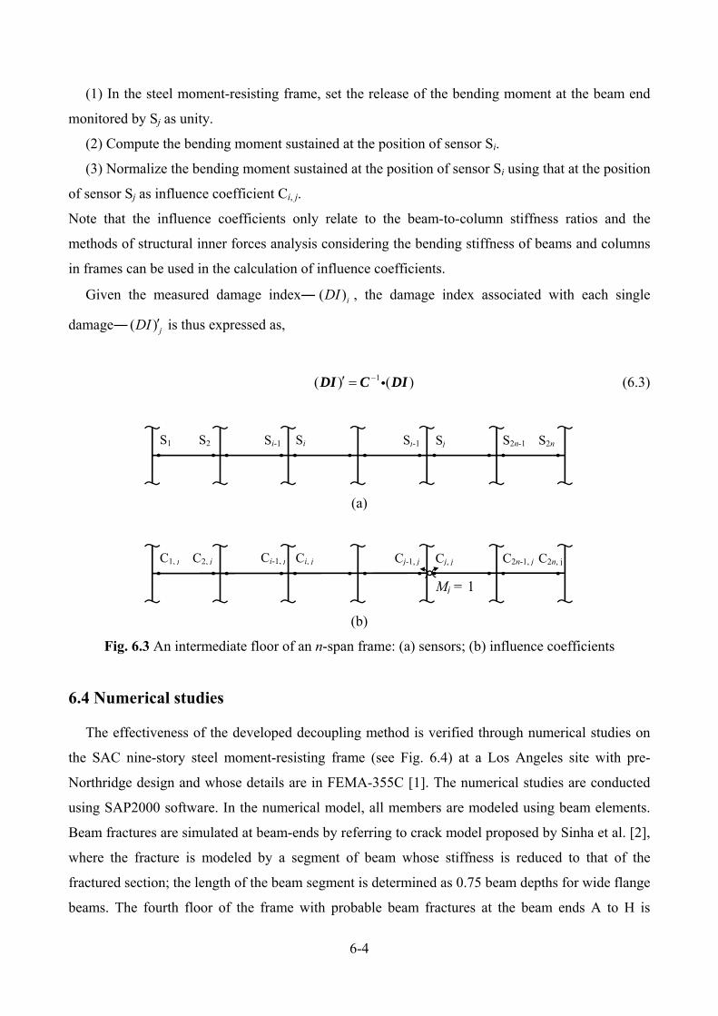
6-4  

(1) In the steel moment-resisting frame, set the release of the bending moment at the beam end

monitored by Sj as unity.

(2) Compute the bending moment sustained at the position of sensor Si.

(3) Normalize the bending moment sustained at the position of sensor Si using that at the position

of sensor Sj as influence coefficient Ci, j.

Note that the influence coefficients only relate to the beam-to-column stiffness ratios and the

methods of structural inner forces analysis considering the bending stiffness of beams and columns

in frames can be used in the calculation of influence coefficients.

Given the measured damage index― ( )iDI , the damage index associated with each single

damage― ( ) jDI is thus expressed as,

1( ) ( ) DI C DI (6.3)

(a)

(b)

Fig. 6.3 An intermediate floor of an n-span frame: (a) sensors; (b) influence coefficients

6.4 Numerical studies

The effectiveness of the developed decoupling method is verified through numerical studies on

the SAC nine-story steel moment-resisting frame (see Fig. 6.4) at a Los Angeles site with pre-

Northridge design and whose details are in FEMA-355C [1]. The numerical studies are conducted

using SAP2000 software. In the numerical model, all members are modeled using beam elements.

Beam fractures are simulated at beam-ends by referring to crack model proposed by Sinha et al. [2],

where the fracture is modeled by a segment of beam whose stiffness is reduced to that of the

fractured section; the length of the beam segment is determined as 0.75 beam depths for wide flange

beams. The fourth floor of the frame with probable beam fractures at the beam ends A to H is

S1 S2 Si Sj-1 S2n-1 S2n SjSi-1

C1, j C2, j Ci, j Cj-1, j C2n-1, j C2n, j Cj, jCi-1, j

Mj = 1

 

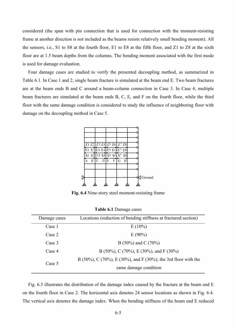
6-5  

considered (the span with pin connection that is used for connection with the moment-resisting

frame at another direction is not included as the beams resists relatively small bending moment). All

the sensors, i.e., S1 to S8 at the fourth floor, E1 to E8 at the fifth floor, and Z1 to Z8 at the sixth

floor are at 1.5 beam depths from the columns. The bending moment associated with the first mode

is used for damage evaluation.

Four damage cases are studied to verify the presented decoupling method, as summarized in

Table 6.1. In Case 1 and 2, single beam fracture is simulated at the beam end E. Two beam fractures

are at the beam ends B and C around a beam-column connection in Case 3. In Case 4, multiple

beam fractures are simulated at the beam ends B, C, E, and F on the fourth floor, while the third

floor with the same damage condition is considered to study the influence of neighboring floor with

damage on the decoupling method in Case 5.

Fig. 6.4 Nine-story steel moment-resisting frame

Table 6.1 Damage cases

Damage cases Locations (reduction of bending stiffness at fractured section)

Case 1 E (10%)

Case 2 E (90%)

Case 3 B (50%) and C (70%)

Case 4 B (50%), C (70%), E (30%), and F (30%)

Case 5 B (50%), C (70%), E (30%), and F (30%); the 3rd floor with the

same damage condition

Fig. 6.5 illustrates the distribution of the damage index caused by the fracture at the beam end E

on the fourth floor in Case 2. The horizontal axis denotes 24 sensor locations as shown in Fig. 6.4.

The vertical axis denotes the damage index. When the bending stiffness of the beam end E reduced

S3 S4 S5

Ground

S1 S2 S6 S7 S8

E1 E2 E3 E4 E5 E6 E7 E8

Z1 Z2 Z3 Z4 Z5 Z6 Z7 Z8

A B C D E F G H

 

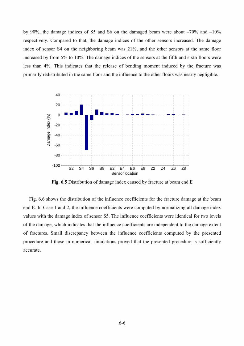
6-6  

by 90%, the damage indices of S5 and S6 on the damaged beam were about ‒70% and ‒10%

respectively. Compared to that, the damage indices of the other sensors increased. The damage

index of sensor S4 on the neighboring beam was 21%, and the other sensors at the same floor

increased by from 5% to 10%. The damage indices of the sensors at the fifth and sixth floors were

less than 4%. This indicates that the release of bending moment induced by the fracture was

primarily redistributed in the same floor and the influence to the other floors was nearly negligible.

Fig. 6.5 Distribution of damage index caused by fracture at beam end E

Fig. 6.6 shows the distribution of the influence coefficients for the fracture damage at the beam

end E. In Case 1 and 2, the influence coefficients were computed by normalizing all damage index

values with the damage index of sensor S5. The influence coefficients were identical for two levels

of the damage, which indicates that the influence coefficients are independent to the damage extent

of fractures. Small discrepancy between the influence coefficients computed by the presented

procedure and those in numerical simulations proved that the presented procedure is sufficiently

accurate.

S2 S4 S6 S8 E2 E4 E6 E8 Z2 Z4 Z6 Z8-100

-80

-60

-40

-20

0

20

40

Sensor location

Da

ma

ge

ind

ex

(%)

 

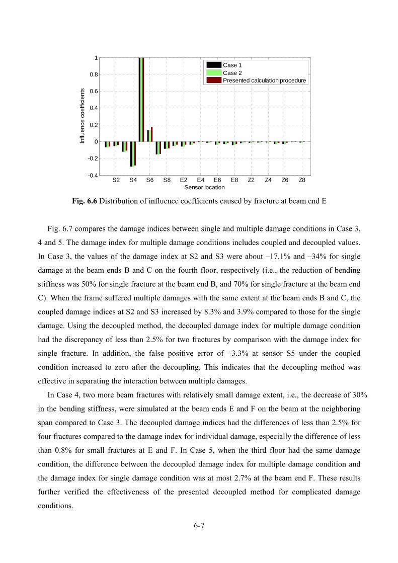
6-7  

Fig. 6.6 Distribution of influence coefficients caused by fracture at beam end E

Fig. 6.7 compares the damage indices between single and multiple damage conditions in Case 3,

4 and 5. The damage index for multiple damage conditions includes coupled and decoupled values.

In Case 3, the values of the damage index at S2 and S3 were about ‒17.1% and ‒34% for single

damage at the beam ends B and C on the fourth floor, respectively (i.e., the reduction of bending

stiffness was 50% for single fracture at the beam end B, and 70% for single fracture at the beam end

C). When the frame suffered multiple damages with the same extent at the beam ends B and C, the

coupled damage indices at S2 and S3 increased by 8.3% and 3.9% compared to those for the single

damage. Using the decoupled method, the decoupled damage index for multiple damage condition

had the discrepancy of less than 2.5% for two fractures by comparison with the damage index for

single fracture. In addition, the false positive error of ‒3.3% at sensor S5 under the coupled

condition increased to zero after the decoupling. This indicates that the decoupling method was

effective in separating the interaction between multiple damages.

In Case 4, two more beam fractures with relatively small damage extent, i.e., the decrease of 30%

in the bending stiffness, were simulated at the beam ends E and F on the beam at the neighboring

span compared to Case 3. The decoupled damage indices had the differences of less than 2.5% for

four fractures compared to the damage index for individual damage, especially the difference of less

than 0.8% for small fractures at E and F. In Case 5, when the third floor had the same damage

condition, the difference between the decoupled damage index for multiple damage condition and

the damage index for single damage condition was at most 2.7% at the beam end F. These results

further verified the effectiveness of the presented decoupled method for complicated damage

conditions.

S2 S4 S6 S8 E2 E4 E6 E8 Z2 Z4 Z6 Z8-0.4

-0.2

0

0.2

0.4

0.6

0.8

1

Sensor location

Influ

en

ce c

oe

ffici

en

ts

Case 1Case 2Presented calculation procedure

 

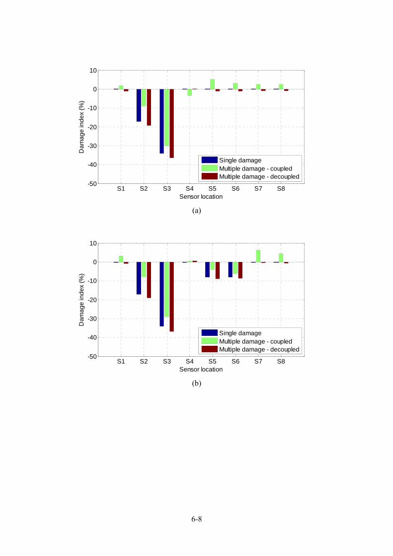
6-8  

(a)

(b)

S1 S2 S3 S4 S5 S6 S7 S8-50

-40

-30

-20

-10

0

10

Sensor location

Da

ma

ge

ind

ex

(%)

Single damageMultiple damage - coupledMultiple damage - decoupled

S1 S2 S3 S4 S5 S6 S7 S8-50

-40

-30

-20

-10

0

10

Sensor location

Da

ma

ge

ind

ex

(%)

Single damageMultiple damage - coupledMultiple damage - decoupled

 

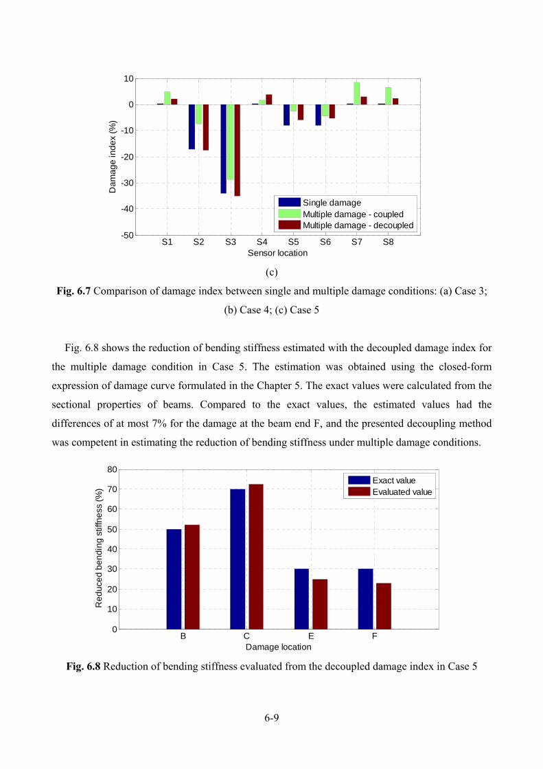
6-9  

(c)

Fig. 6.7 Comparison of damage index between single and multiple damage conditions: (a) Case 3;

(b) Case 4; (c) Case 5

Fig. 6.8 shows the reduction of bending stiffness estimated with the decoupled damage index for

the multiple damage condition in Case 5. The estimation was obtained using the closed-form

expression of damage curve formulated in the Chapter 5. The exact values were calculated from the

sectional properties of beams. Compared to the exact values, the estimated values had the

differences of at most 7% for the damage at the beam end F, and the presented decoupling method

was competent in estimating the reduction of bending stiffness under multiple damage conditions.

Fig. 6.8 Reduction of bending stiffness evaluated from the decoupled damage index in Case 5

S1 S2 S3 S4 S5 S6 S7 S8-50

-40

-30

-20

-10

0

10

Sensor location

Da

ma

ge

ind

ex

(%)

Single damageMultiple damage - coupledMultiple damage - decoupled

B C E F0

10

20

30

40

50

60

70

80

Damage location

Re

du

ced

be

nd

ing

stif

fne

ss (

%)

Exact valueEvaluated value

 

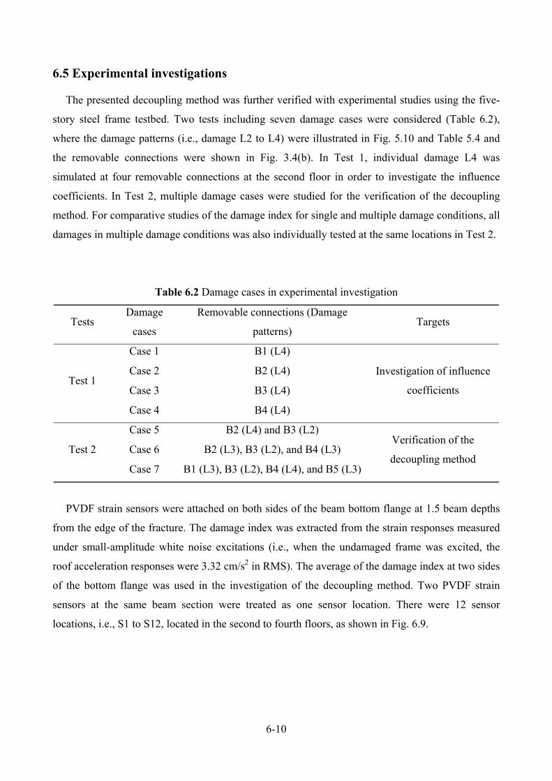
6-10  

6.5 Experimental investigations

The presented decoupling method was further verified with experimental studies using the five-

story steel frame testbed. Two tests including seven damage cases were considered (Table 6.2),

where the damage patterns (i.e., damage L2 to L4) were illustrated in Fig. 5.10 and Table 5.4 and

the removable connections were shown in Fig. 3.4(b). In Test 1, individual damage L4 was

simulated at four removable connections at the second floor in order to investigate the influence

coefficients. In Test 2, multiple damage cases were studied for the verification of the decoupling

method. For comparative studies of the damage index for single and multiple damage conditions, all

damages in multiple damage conditions was also individually tested at the same locations in Test 2.

Table 6.2 Damage cases in experimental investigation

Tests Damage

cases

Removable connections (Damage

patterns) Targets

Test 1

Case 1 B1 (L4)

Investigation of influence

coefficients

Case 2 B2 (L4)

Case 3 B3 (L4)

Case 4 B4 (L4)

Test 2

Case 5 B2 (L4) and B3 (L2) Verification of the

decoupling method Case 6 B2 (L3), B3 (L2), and B4 (L3)

Case 7 B1 (L3), B3 (L2), B4 (L4), and B5 (L3)

PVDF strain sensors were attached on both sides of the beam bottom flange at 1.5 beam depths

from the edge of the fracture. The damage index was extracted from the strain responses measured

under small-amplitude white noise excitations (i.e., when the undamaged frame was excited, the

roof acceleration responses were 3.32 cm/s2 in RMS). The average of the damage index at two sides

of the bottom flange was used in the investigation of the decoupling method. Two PVDF strain

sensors at the same beam section were treated as one sensor location. There were 12 sensor

locations, i.e., S1 to S12, located in the second to fourth floors, as shown in Fig. 6.9.

 

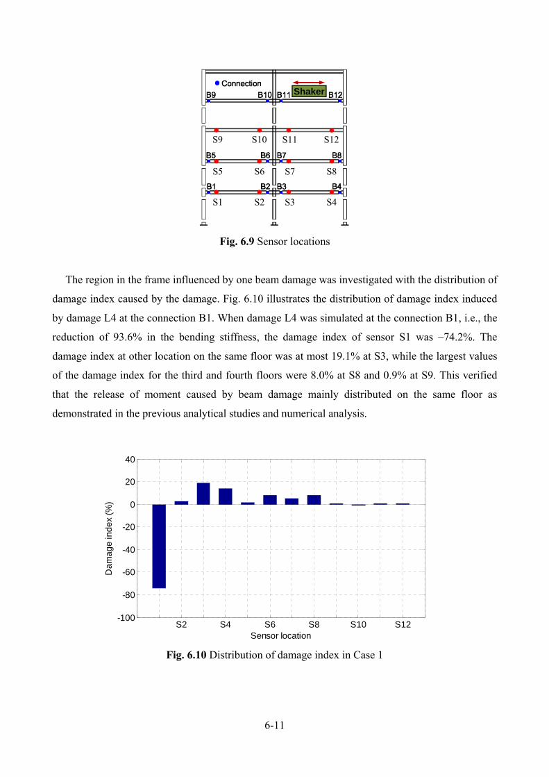
6-11  

Fig. 6.9 Sensor locations

The region in the frame influenced by one beam damage was investigated with the distribution of

damage index caused by the damage. Fig. 6.10 illustrates the distribution of damage index induced

by damage L4 at the connection B1. When damage L4 was simulated at the connection B1, i.e., the

reduction of 93.6% in the bending stiffness, the damage index of sensor S1 was ‒74.2%. The

damage index at other location on the same floor was at most 19.1% at S3, while the largest values

of the damage index for the third and fourth floors were 8.0% at S8 and 0.9% at S9. This verified

that the release of moment caused by beam damage mainly distributed on the same floor as

demonstrated in the previous analytical studies and numerical analysis.

Fig. 6.10 Distribution of damage index in Case 1

S2 S4 S6 S8 S10 S12-100

-80

-60

-40

-20

0

20

40

Sensor location

Da

ma

ge

ind

ex

(%)

Shaker

S1 S2 S3 S4

S5 S6 S7 S8

S9 S10 S11 S12

 

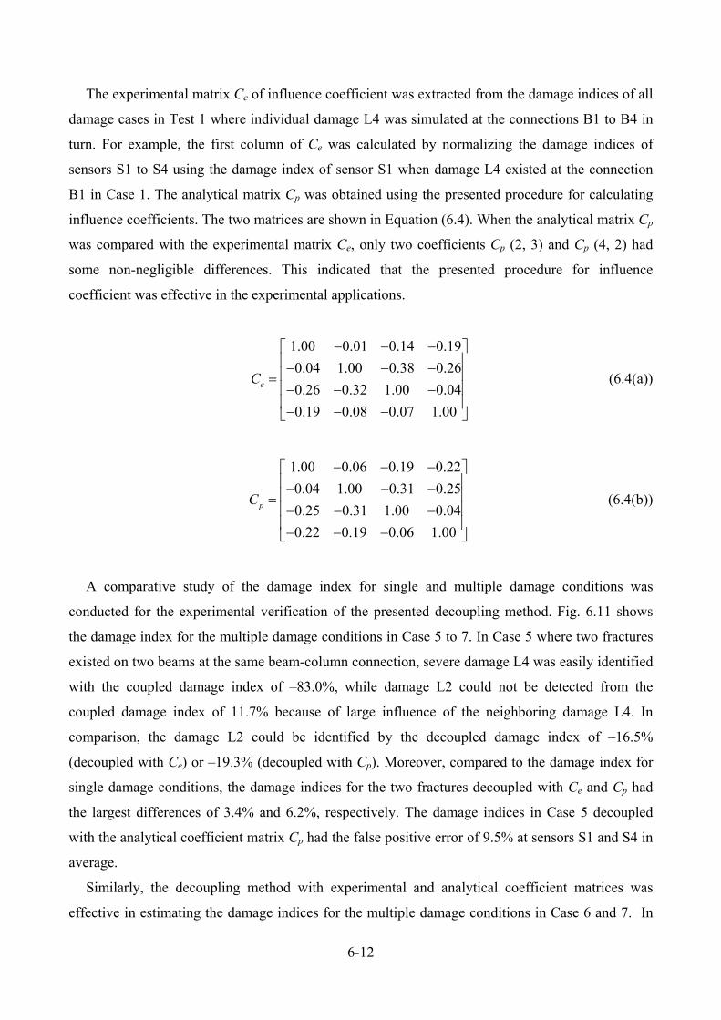
6-12  

The experimental matrix Ce of influence coefficient was extracted from the damage indices of all

damage cases in Test 1 where individual damage L4 was simulated at the connections B1 to B4 in

turn. For example, the first column of Ce was calculated by normalizing the damage indices of

sensors S1 to S4 using the damage index of sensor S1 when damage L4 existed at the connection

B1 in Case 1. The analytical matrix Cp was obtained using the presented procedure for calculating

influence coefficients. The two matrices are shown in Equation (6.4). When the analytical matrix Cp

was compared with the experimental matrix Ce, only two coefficients Cp (2, 3) and Cp (4, 2) had

some non-negligible differences. This indicated that the presented procedure for influence

coefficient was effective in the experimental applications.

1.00 0.01 0.14 0.19

0.04 1.00 0.38 0.26

0.26 0.32 1.00 0.04

0.19 0.08 0.07 1.00

eC

(6.4(a))

1.00 0.06 0.19 0.22

0.04 1.00 0.31 0.25

0.25 0.31 1.00 0.04

0.22 0.19 0.06 1.00

pC

(6.4(b))

A comparative study of the damage index for single and multiple damage conditions was

conducted for the experimental verification of the presented decoupling method. Fig. 6.11 shows

the damage index for the multiple damage conditions in Case 5 to 7. In Case 5 where two fractures

existed on two beams at the same beam-column connection, severe damage L4 was easily identified

with the coupled damage index of ‒83.0%, while damage L2 could not be detected from the

coupled damage index of 11.7% because of large influence of the neighboring damage L4. In

comparison, the damage L2 could be identified by the decoupled damage index of ‒16.5%

(decoupled with Ce) or ‒19.3% (decoupled with Cp). Moreover, compared to the damage index for

single damage conditions, the damage indices for the two fractures decoupled with Ce and Cp had

the largest differences of 3.4% and 6.2%, respectively. The damage indices in Case 5 decoupled

with the analytical coefficient matrix Cp had the false positive error of 9.5% at sensors S1 and S4 in

average.

Similarly, the decoupling method with experimental and analytical coefficient matrices was

effective in estimating the damage indices for the multiple damage conditions in Case 6 and 7. In

 

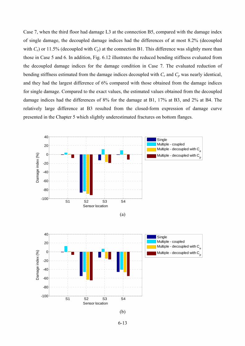
6-13  

Case 7, when the third floor had damage L3 at the connection B5, compared with the damage index

of single damage, the decoupled damage indices had the differences of at most 8.2% (decoupled

with Ce) or 11.5% (decoupled with Cp) at the connection B1. This difference was slightly more than

those in Case 5 and 6. In addition, Fig. 6.12 illustrates the reduced bending stiffness evaluated from

the decoupled damage indices for the damage condition in Case 7. The evaluated reduction of

bending stiffness estimated from the damage indices decoupled with Ce and Cp was nearly identical,

and they had the largest difference of 6% compared with those obtained from the damage indices

for single damage. Compared to the exact values, the estimated values obtained from the decoupled

damage indices had the differences of 8% for the damage at B1, 17% at B3, and 2% at B4. The

relatively large difference at B3 resulted from the closed-form expression of damage curve

presented in the Chapter 5 which slightly underestimated fractures on bottom flanges.

(a)

(b)

S1 S2 S3 S4-100

-80

-60

-40

-20

0

20

40

Sensor location

Da

ma

ge

ind

ex

(%)

SingleMultiple - coupledMultiple - decoupled with C

e

Multiple - decoupled with Cp

S1 S2 S3 S4-100

-80

-60

-40

-20

0

20

40

Sensor location

Da

ma

ge

ind

ex

(%)

SingleMultiple - coupledMultiple - decoupled with C

e

Multiple - decoupled with Cp

 

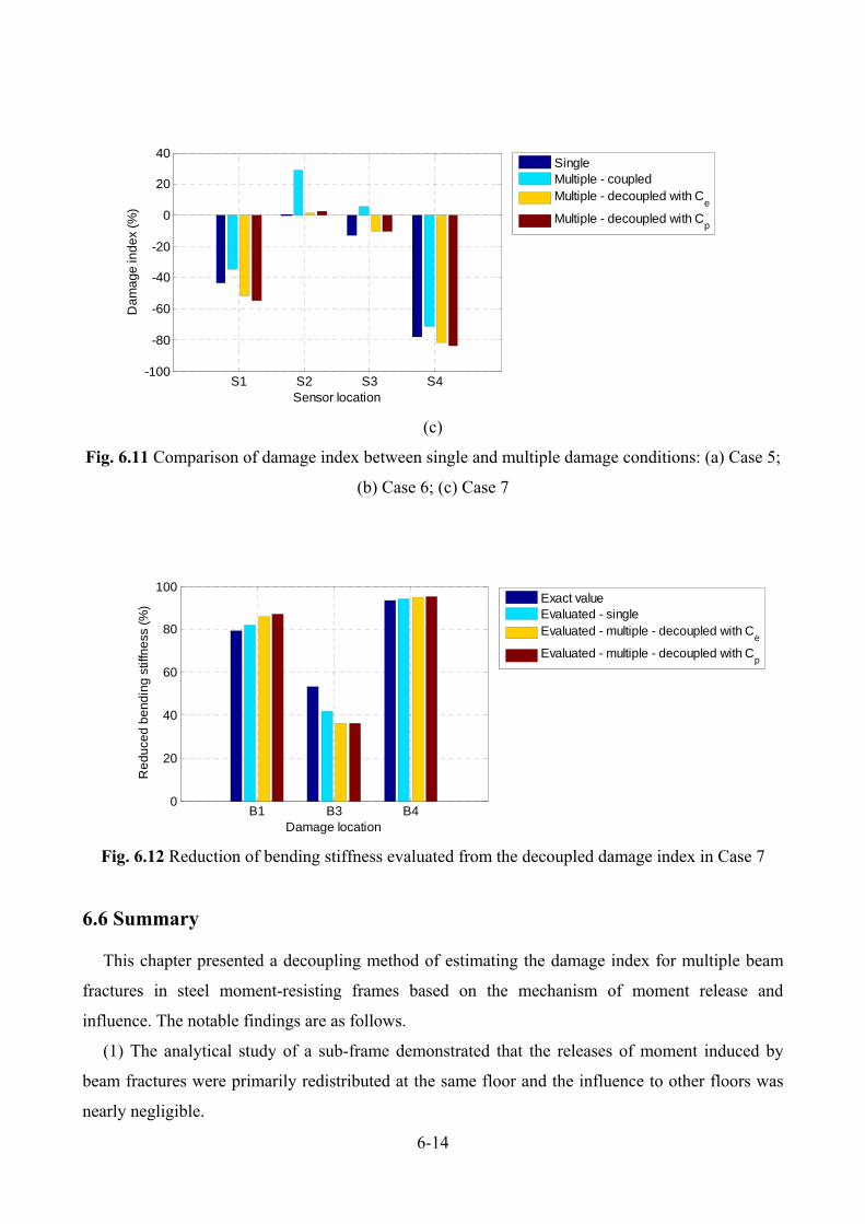
6-14  

(c)

Fig. 6.11 Comparison of damage index between single and multiple damage conditions: (a) Case 5;

(b) Case 6; (c) Case 7

Fig. 6.12 Reduction of bending stiffness evaluated from the decoupled damage index in Case 7

6.6 Summary

This chapter presented a decoupling method of estimating the damage index for multiple beam

fractures in steel moment-resisting frames based on the mechanism of moment release and

influence. The notable findings are as follows.

(1) The analytical study of a sub-frame demonstrated that the releases of moment induced by

beam fractures were primarily redistributed at the same floor and the influence to other floors was

nearly negligible.

S1 S2 S3 S4-100

-80

-60

-40

-20

0

20

40

Sensor location

Da

ma

ge

ind

ex

(%)

SingleMultiple - coupledMultiple - decoupled with C

e

Multiple - decoupled with Cp

B1 B3 B40

20

40

60

80

100

Damage location

Re

du

ced

be

nd

ing

stif

fne

ss (

%)

Exact valueEvaluated - singleEvaluated - multiple - decoupled with C

e

Evaluated - multiple - decoupled with Cp

 

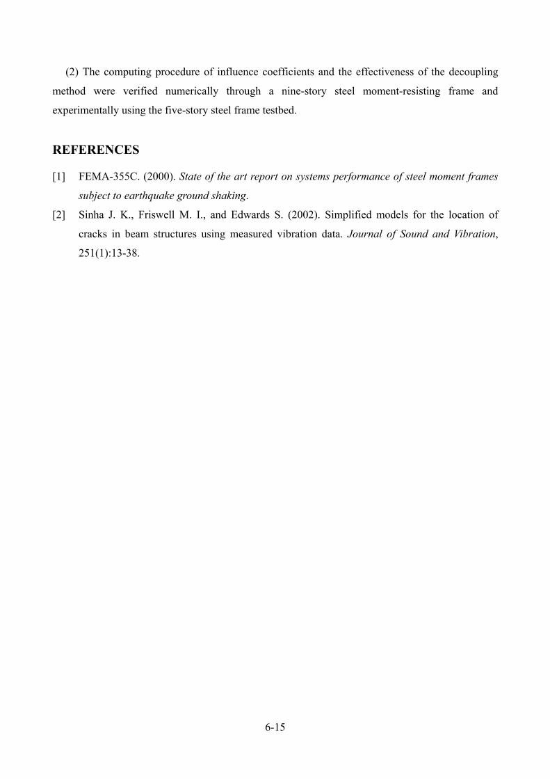
6-15  

(2) The computing procedure of influence coefficients and the effectiveness of the decoupling

method were verified numerically through a nine-story steel moment-resisting frame and

experimentally using the five-story steel frame testbed.

REFERENCES

[1] FEMA-355C. (2000). State of the art report on systems performance of steel moment frames

subject to earthquake ground shaking.

[2] Sinha J. K., Friswell M. I., and Edwards S. (2002). Simplified models for the location of

cracks in beam structures using measured vibration data. Journal of Sound and Vibration,

251(1):13-38.

 

6-16  

 

7-1  

CHAPTER 7

Conclusions and future studies

7.1 Conclusions

This dissertation developed a localized damage evaluation method specifically designed for

detecting and quantifying seismically-induced beam fractures to beam-to-column connections in

steel moment-resisting frames. The proposed method would facilitate rapid and reliable estimation

on the remaining capacity of the earthquake-affected steel buildings and thus support post-quake

decision-making on re-occupancy. The effectiveness of the method was investigated through

numerical studies with a nine-story steel moment-resisting frame and experimental studies using the

five-story steel frame testbed. In this dissertation, the notable findings are summarized as follows.

Chapter 2: Concept of local damage evaluation

(1) In steel moment-resisting frames, local damage such as seismically-induced fractures on steel

beams changes the distribution of bending moments sustained by members. In practice, when the

frames behave linearly under small amplitude vibrations, the bending moments can be estimated by

measuring strain responses on the members. Based on these physical mechanisms, a concept of

seismically-induced local damage evaluation method using wireless piezoelectric strain sensing was

presented.

Chapter 3: Strain-based damage index

(1) A novel damage index was formulated using a comparative study of the bending strain

responses of beams associated with a natural mode between the undamaged and damaged frames.

The damage index was proved to be independent of external excitations and vibrational modes.

 

7-2  

(2) The developed wireless piezoelectric strain sensing system, comprised of PVDF sensors and

Narada wireless units, showed excellent performance for monitoring the dynamic strain in the steel

structures under small amplitude vibrations and even ambient excitations.

(3) In the experimental results for the five-story steel frame testbed, variation in the damage

index under the undamaged conditions was less than 7% for different excitations, and weak

dependency of damage index on the characteristics of the external excitations was preliminarily

verified.

(4) Damaged locations were successfully identified in the tests using the distribution of damage

index values. Moreover, the damage index values for various severity levels showed clear discrete

values that would enable the quantification of seismic fracture damage.

Chapter 4: Sensitivity investigation of the damage index

(1) Independency of the presented damage index on the characteristics of external excitations

and the selection of vibration modes was verified in numerical simulations and shaking table tests.

As the extraction of modal responses required preset band-pass filters, the use of dominant vibration

modes with clear responses and high power was highly desirable.

(2) Both in the numerical simulations and experiments, the damage index extracted from a

distance not more than 1.2d (d is the beam depth) from a fracture was largely affected by local

strain redistributions induced by the fracture. A distance between 1.2d and 2.0d from the fracture

was recommended for evaluating the moment redistributions in steel moment-resisting frames and

the reduction in bending stiffness at fractured sections.

(3) Consistency of the damage index in the evaluation of damage at different locations was

verified in experimental studies using the five-story steel testbed frame. The level of variation was

at most 7.8% for fracture on the bottom flange, and 3.8% for fracture of the bottom flange and web.

(4) The increases of the damage index at damage-neighboring connections were verified using a

preliminary experimental study considering multiple damage conditions. The interaction between

neighboring damage at the same beam-column connections was much more significant than that

observed at different connections.

Chapter 5: Simplified derivation of damage curve

(1) A closed-form expression of damage curve was derived from an analytical parametric study

using a two-story two-bay frame. The damage curve was a relationship that represents the strain-

based damage index as a function of the reduction in beam bending stiffness induced by fracture.

 

7-3  

(2) The presented damage curve was dominated primarily by the span-depth ratio of fractured

beam and hardly affected by the other structural parameters, such as the height ratio between stories,

the column-to-beam stiffness ratio, and the lateral force ratio between floors.

(3) The damage curve was demonstrated to be capable of evaluating the amount of earthquake-

induced fractures on beams for common multi-story multi-bay steel moment-resisting frames

through numerical studies conducted for a nine-story steel moment-resisting frame and

experimental investigations using a one-quarter-scale five-story steel frame testbed.

Chapter 6: Decoupling interaction between multiple damage

(1) An analytical study of a sub-frame demonstrated that the releases of moment induced by

beam fractures were primarily redistributed at the same floor and the influence to other floors was

nearly negligible.

(2) A decoupling method of estimating the damage index for multiple beam fractures was

presented based on the mechanism of moment release and influence.

(3) The effectiveness of the decoupling method was verified numerically through a nine-story

steel moment-resisting frame and experimentally using the five-story steel frame testbed.

7.2 Future studies

The proposed method in this dissertation is a strategy for local damage evaluation in steel

moment-resisting frames, which provides damage information (i.e., existence, location, and extent)

of the monitored beams and thus potentially supports rapid post-earthquake damage assessment and

decision-making on re-occupancy for the earthquake-affected steel buildings.

Future studies are needed to develop a prototype of rapid post-earthquake damage and safety

evaluation program by integrating global characteristics with local damage information for steel

moment-resisting frames. The notable features and functions of the program will be (1) instant

inspection of local damage, (2) rapid assessment of damage state, (3) re-occupancy safety

evaluation based on identified local damage. The program will be capable of providing reliable

damage and safety information to support decision making on re-occupancy and recovery. Proposed

topics are as follows.

(1)  Damage state assessment using story drift-based fragility functions updated with local

damage information

 

7-4  

As illustrated in the CSMIP-3DV [1] software systems, the drift-based fragility functions derived

from experimental data for structural components is widely used in the SHM-based post-earthquake

damage condition assessment. Once the story drift is obtained from measured data, the probability

of damage state for floor levels and entire buildings can be estimated through fragility functions.

Nonetheless, in steel moment-resisting frames, because of the hysteresis behaviors of members and

connections involving large uncertainties, the story drift-based fragility functions are not necessarily

effective in damage assessment. For instance, a story experiencing an inter-story drift of 1.5% has a

5% probability of not having damage, 44% of having slight damage, 46% of experiencing moderate

damage, and 5% of sustaining severe damage. This result would make decision makers indecisive.

The local damage identified with the presented local damage evaluation method is evidence of

damage in buildings. This valuable information can be used to update the developed fragility

functions with Bayesian inference to reduce uncertainties. With this background, a method of

updating story drift-based fragility function with identified local damage information for rapid

damage condition assessment will be studied.

(2) Re-occupancy safety evaluation based on identified local damage

After a damaging earthquake, when an earthquake-affected building undergoes local damage on

structural members that are identified through a health monitoring system, most important is to

determine if the identified damage affects the structural safety of the buildings for re-occupancy.

Except the buildings suffered obviously severe damage and near collapse, other buildings need to

be assessed on their ability to resist future loadings. The commonly accepted evaluation approaches

for seismic safety are based mainly on the residual strength and stiffness of the damaged buildings

relative to the current code requirements and pre-earthquake conditions, and the probability of

collapse of the damaged buildings induced by a given hazard (usually 50% chance of exceedance in

50 years). Thus, the safety evaluation methods based on residual capacity (i.e., strength and

stiffness) and probability of collapse under a given hazard will be investigated and their feasibility

for application to the proposed program will be studied.

(3) Design of rapid post-earthquake damage and safety evaluation program

Compared to existing programs where only damage condition information estimated from global

characteristics is provided for post-earthquake decision-making, the proposed program will be

designed to further include local damage-based damage condition assessment and safety estimation.

This program will achieve two-stage assessments: rapid damage state assessment and re-occupancy

safety evaluation. For instance, after an earthquake, the program immediately conducts the rapid

 

7-5  

damage state assessment. If the building probably experienced unsafe damage state, the program

warns the users in the building to evacuate in a short time. Then, the program continues the re-

occupancy safety evaluation. If the building keeps 90% of the capacity compared to the pre-

earthquake condition, the decision makers may make the judgement of re-occupancy. To realize

these functions in the proposed program, a framework and procedure of the rapid post-earthquake

damage and safety evaluation program and the design of an associated computer program will be

studied.

REFERENCES

[1] Naeim F., Hagie H., Alimoradi A., and Miranda E. (2005). Automated post-earthquake

damage assessment and safety evaluation of instrumented buildings. A Report to CSMIP

(JAMA Report No. 2005–10639), John A. Martin & Associates.

 

7-6  

 

I  

Acknowledgments

I would like to express my sincere gratitude to the many people who helped in the preparation of

this doctoral dissertation.

Professor Masayoshi Nakashima, my supervisor of the doctoral research. With his guidance,

encouragements, and unlimited supports, all went smoothly during my doctoral study. In

addition, I am most grateful for his patience to my many flaws. His enthusiasm, critical

thinking, and rigorous attitude to research also affected me a lot. It is a great honor to be his

student.

Professor Masahiro Kurata, my vice-supervisor for this dissertation. From beginning to end,

he spent extensive time and labor on this research. He discussed this research with me

weekly, and provided substantive suggestions and insightful comments. I really appreciate

his limitless help and supports to complete this research, and many works in the

experiments, writing, and publication.

Two members of the dissertation committee: Professor Izuru Takewaki and Professor

Hiroshi Kawase. They reviewed this thesis, and provided many perceptive suggestions for

improvement.

Mrs Chisato Gamou. I am grateful for her much assistance in office affairs.

SHM group members: Professor Kohei Fujita, Dr Tang Zhenyun, Dr Bai Yongtao, Ms

Mayako Yamaguchi, Ms Kaede Minegishi, Ms Akiko Suzuki, Mr Hiromichi Nishino, and

Mr Shota Shinmoto. They helped each experimental investigation, and discussed with me

each problem. From them, I learned a lot.

Student members in Nakashima-Kurata lab: Dr Takehiko Asai, Dr Hongsong Hu, Dr

Konstantinos Skalomenos, Ms Francesca Barbagallo, Mr Lei Zhang, Mr Hiroyuki Inamasu,

Ms Miho Sato, Ms Ikumi Hamashima, Mr Yu Otsuki, Mr Hironari Shimada, Mr Tadahisa

Takeda, Mr Deng Kailai, Dr Kazuhiro Hayashi, Dr Po-Chien Hsiao, Dr Xuchuan Lin, Dr

Yundong Shi, Dr Yunbiao Luo, Dr Liusheng He, Mr. Ryosuke Nishi, Mr. Takuma Togo and

so on. They helped a lot in my research and daily life. We had many happy moments and

shared much interesting experience.

Ministry of Education, Culture, Sports, Science and Technology (MEXT), Japan. MEXT

provided four-year scholarship for my study in Japan.

 

II  

My family. I am very grateful to my parents and my brother for their endless love, supports,

encouragements, and concerns during my study in Japan.

June 13th, 2015

Xiaohua Li