evaluation of air quality models with near-road monitoring
TRANSCRIPT

Cooperative Research Program
TTI: 0-6943
Technical Report 0-6943-R1
Evaluation of Air Quality Models with Near-Road
Monitoring Data: Technical Report
in cooperation with the
Federal Highway Administration and the
Texas Department of Transportation
http://tti.tamu.edu/documents/0-6943-R1.pdf
TEXAS A&M TRANSPORTATION INSTITUTE
COLLEGE STATION, TEXAS


Technical Report Documentation Page 1. Report No.
FHWA/TX-20/0-6943-R1
2. Government Accession No.
3. Recipient's Catalog No.
4. Title and Subtitle
EVALUATION OF AIR QUALITY MODELS WITH NEAR-ROAD
MONITORING DATA: TECHNICAL REPORT
5. Report Date
Published: October 2020 6. Performing Organization Code
7. Author(s)
Reza Farzaneh, Suriya Vallamsundar, Rohit Jaikumar, Madhu Venugopal,
Mohammad Askariyeh, Jeremy Johnson, Wen-Whai Li, Mayra C. Chavez,
and Ivan M. Ramirez
8. Performing Organization Report No.
Report 0-6943-R1
9. Performing Organization Name and Address
Texas A&M Transportation Institute
The Texas A&M University System
College Station, Texas 77843-3135
10. Work Unit No. (TRAIS)
11. Contract or Grant No.
Project 0-6943 12. Sponsoring Agency Name and Address
Texas Department of Transportation
Research and Technology Implementation Office
125 E. 11th Street
Austin, Texas 78701-2483
13. Type of Report and Period Covered
Technical Report:
November 2016–August 2019 14. Sponsoring Agency Code
15. Supplementary Notes
Project performed in cooperation with the Texas Department of Transportation and the Federal Highway
Administration.
Project Title: Evaluation of Air Quality Models with Near-Road Monitoring Data
URL: http://tti.tamu.edu/documents/0-6943-R1.pdf 16. Abstract
Air dispersion models (air quality models) are used in evaluation of transportation projects to ensure their compliance
with federal regulations including the National Environmental Policy Act and transportation conformity quantitative
hot-spot analysis requirements. The literature indicates a wide range of variabilities involved in the modeling process
for the particulate matter (PM) hot-spot analysis. Sparse real-world data have limited the ability to evaluate the
variabilities involved in the PM hot-spot analysis process. Availability of near-road monitoring data has provided a
new source of data to address this gap.
The objective of this study was to perform a modeling evaluation of the regulatory hot spot analysis and conduct a data
research of the near-road monitoring observations to evaluate the potential association between the near-road PM2.5
concentrations and the key parameters. The study was performed for two case study sites in Texas, namely Houston
and Fort Worth. The modeling process evaluation consisted of investigating the model behavior and variabilities
involved in the PM2.5 hot-spot process through a series of sensitivity analyses.
The results of the modeling variability analysis highlighted significant variations of the estimated near-road
concentrations as a result of typical modeling options and data sources used in conducting a PM2.5 hot-spot analysis.
The range of variability was highest for the model options, followed by model choice, and data source. In addition to
sensitivity analysis, the data exploration indicated that the background concentration is the dominating factor in
estimating the near-road PM2.5 concentrations. Traffic volume and speed were found to have a relatively weak
association with the near-road concentrations of PM2.5 for the two case study sites. Wind direction and speed were
found to have a stronger association with the concentrations; however, the lack of hourly near-road concentration data
at the time of this study prevented a detailed analysis of this potential correlation at an hourly resolution. 17. Key Words
Near-road, Monitoring, Air Dispersion, AERMOD,
CAL3QHCR, Data Research, Particulate Matter, Hot-
Spot Analysis, Model Evaluation, and Sensitivity
Analysis, Transportation Conformity, NEPA
18. Distribution Statement
No restrictions. This document is available to the public
through NTIS:
National Technical Information Service
Alexandria, Virginia
http://www.ntis.gov 19. Security Classif. (of this report)
Unclassified
20. Security Classif. (of this page)
Unclassified
21. No. of Pages
170
22. Price
Form DOT F 1700.7 (8-72) Reproduction of completed page authorized


EVALUATION OF AIR QUALITY MODELS WITH NEAR-ROAD
MONITORING DATA: TECHNICAL REPORT
by
Reza Farzaneh
Associate Research Engineer
Suriya Vallamsundar
Assistant Research Scientist
Rohit Jaikumar
Associate Transportation Researcher
Madhu Venugopal
Associate Research Scientist
Mohammad Askariyeh
Graduate Assistant in Research
Jeremy Johnson
Research Specialist II
Texas A&M Transportation Institute
and
Wen-Whai Li
Professor
Mayra C. Chavez
Graduate Research Associate
Ivan M. Ramirez
Graduate Research Assistant
The University of Texas at El Paso
Report 0-6943-R1
Project 0-6943
Project Title: Evaluation of Air Quality Models with Near-Road Monitoring Data
Performed in cooperation with the
Texas Department of Transportation
and the Federal Highway Administration
Published: October 2020
TEXAS A&M TRANSPORTATION INSTITUTE
College Station, Texas 77843-3135


v
DISCLAIMER
This research was performed in cooperation with the Texas Department of Transportation
(TxDOT) and the Federal Highway Administration (FHWA). The contents of this report reflect
the views of the authors, who are responsible for the facts and the accuracy of the data presented
herein. The contents do not necessarily reflect the official view or policies of the FHWA or
TxDOT. This report does not constitute a standard, specification, or regulation.
The United States Government and the State of Texas do not endorse products or manufacturers.
Trade or manufacturers’ names appear herein solely because they are considered essential to the
object of this report.

vi
ACKNOWLEDGMENTS
This project was conducted in cooperation with TxDOT and FHWA. The authors thank the
Project Manager, Wade Odell, and the Project Committee, Jackie Ploch and Tim Wood from
TxDOT, and Michael Claggett from FHWA for their guidance and oversight during the course of
this project. Authors also thank their TTI colleagues Bob Huch and Bahar Dadashova for their
help on the data exploration tasks, and Tara Ramani, Jolanda Prozzi, and Joe Zietsman for their
support throughout the study. Authors also thank the North Central Texas Council of
Governments (NCTCOG), and Houston-Galveston Area Council (HGAC) for their help with the
travel demand model inputs.

vii
TABLE OF CONTENTS
Page
List of Figures ................................................................................................................................ x List of Tables ............................................................................................................................... xii Chapter 1: Introduction ............................................................................................................... 1
Background and Research Goal .................................................................................................. 1 Project Scope and Context .......................................................................................................... 3
Research Plan .............................................................................................................................. 4 Organization of Report ............................................................................................................... 5
Chapter 2: Literature Review and State-of-Practice ................................................................. 7
Introduction ................................................................................................................................. 7 Air Quality Models and Regulatory Context .............................................................................. 7
Air Dispersion Models ............................................................................................................ 7
Regulatory Context of Dispersion Models.............................................................................. 8 CALINE3 Series and AERMOD Model Description and Evolution ..................................... 9 Review of Studies on Model Evaluation............................................................................... 10
Key Components of PM Hot-Spot Analysis ............................................................................. 16 Overall Framework ............................................................................................................... 17
Traffic Data Characterization ............................................................................................... 18 Emission Modeling ............................................................................................................... 20
Near-Road Air Quality .............................................................................................................. 25
Near-Road Pollutant Concentrations .................................................................................... 26 Near-Road Monitoring Stations and Regulatory Processes .................................................. 27
Review of Studies Focusing on Near-Road Data.................................................................. 29 Summary ................................................................................................................................... 32
Chapter 3: Study Design and Case Study Protocols ................................................................ 33 Introduction ............................................................................................................................... 33 Methodology ............................................................................................................................. 33
Data Selection Metrics .............................................................................................................. 34 Input Data ................................................................................................................................. 37
Track 1: Data Exploration Research ..................................................................................... 38
Track 2: Modeling ................................................................................................................. 39 Summary ................................................................................................................................... 42
Chapter 4: Data Exploration Research..................................................................................... 43 Introduction ............................................................................................................................... 43
Methods and Data ..................................................................................................................... 43 Methods ................................................................................................................................. 43 Data Acquisition ................................................................................................................... 44
Results ....................................................................................................................................... 50 Distribution of Near-Road Pollutants ................................................................................... 51 Near-Road Concentration and Meteorology ......................................................................... 52 Near-Road Concentration and Traffic Activity .................................................................... 56 Near-Road and Background Concentrations......................................................................... 60 Correlation Matrix ................................................................................................................ 64

viii
Summary ................................................................................................................................... 67 Chapter 5: Modeling Approach and Data ................................................................................ 69
Introduction ............................................................................................................................... 69 Traffic Activity Data ................................................................................................................. 70 MOVES Modeling .................................................................................................................... 71 Air Dispersion Modeling .......................................................................................................... 73
Step 1 .................................................................................................................................... 73
Step 2 .................................................................................................................................... 75 Step 3 .................................................................................................................................... 76
Background Concentration ....................................................................................................... 76 Method 1: Single Station Estimate ....................................................................................... 77 Method 2: Arithmetic Mean .................................................................................................. 77
Method 3: Weighted Mean Estimate by Inverse Distance .................................................... 78
Method 4: Weighted Mean by Inverse Distance Squared..................................................... 78 Method 5: Normalized Arithmetic Mean Estimate ............................................................... 78
Other Tools and Methods ......................................................................................................... 79
Summary ................................................................................................................................... 81 Chapter 6: Modeling Scenarios and Results ............................................................................ 83
Introduction ............................................................................................................................... 83
Modeling Scenarios .................................................................................................................. 83 Traffic Data Characterization ............................................................................................... 83
Emission Modeling ............................................................................................................... 84 Meteorological Data Processing ........................................................................................... 84 Air Dispersion Modeling ...................................................................................................... 85
Model Set-up ............................................................................................................................. 87
Modeling Results ...................................................................................................................... 93 Traffic Activity Data ............................................................................................................. 94 MOVES Modeling ................................................................................................................ 95
Meteorology .......................................................................................................................... 95 Land Use ............................................................................................................................... 95
Air Dispersion Parameters .................................................................................................... 96 Summary ................................................................................................................................... 97
Chapter 7: Qualitative Evaluation ............................................................................................ 99
Introduction ............................................................................................................................... 99 Modeling Scenarios .................................................................................................................. 99 Design Values and Hot-Spot Analysis .................................................................................... 100
Key Findings ........................................................................................................................... 116 Chapter 8: Findings and Conclusions ..................................................................................... 119
Track 1—Data Exploration ..................................................................................................... 119 Track 2—Modeling Sensitivity Analysis ............................................................................... 120
References .................................................................................................................................. 123 Appendix A: Meteorological Data ........................................................................................... 131
Meteorological Data Processing for AERMOD ..................................................................... 131
Meteorological Files Required by AERMET ..................................................................... 132 Meteorological Files Generated by AERMET.................................................................... 134
Meteorological Data Processing for CAL3QHCR ................................................................. 134

ix
Consistency between AERMET and PCRAMMET Outputs ................................................. 137 Appendix B: Background Concentration ............................................................................... 139
Results and Discussion ........................................................................................................... 139 Annual Average PM2.5 Concentrations ................................................................................... 139 24-hr Average PM2.5 Concentrations ...................................................................................... 142 Highest Ten 24-hr Average PM2.5 Concentrations ................................................................. 143
Appendix C: Time Series Plots ................................................................................................ 147
Traffic Aggregation ................................................................................................................ 147 Meteorological Data ............................................................................................................... 150 Source Type ............................................................................................................................ 153 Land Use ................................................................................................................................. 154 Model Choice: CAL3QHCR, Met Data ................................................................................. 155

x
LIST OF FIGURES
Page
Figure 1. Project Tasks. .................................................................................................................. 5 Figure 2. Overall Modeling Framework. ...................................................................................... 18 Figure 3. Traffic Data Sources and Uses. ..................................................................................... 19 Figure 4. MOVES Emission Modeling. ........................................................................................ 21 Figure 5. Air Dispersion Modeling Process. ................................................................................. 22
Figure 6. Near-Road and Ambient Monitoring Stations in Texas. ............................................... 28 Figure 7. Overall Modeling Framework. ...................................................................................... 34 Figure 8. Key Differences between Track 1 and Track 2. ............................................................ 41
Figure 9. Study Design: Track 1 and Track 2. .............................................................................. 42 Figure 10. Near-Road and Ambient Monitoring Stations in Texas. ............................................. 44 Figure 11. Location of Houston Near-Road Monitoring Station. ................................................. 45
Figure 12. Location of Fort Worth Near-Road Monitoring Station. ............................................. 46 Figure 13. Location of TxDOT (STARS-II) Traffic Counters near Houston Monitor. ................ 47 Figure 14. Location of TxDOT (STARS-II) Traffic Counter near Fort Worth Monitor. ............. 48
Figure 15. Ambient Monitoring Stations Surrounding Houston Near-Road Monitor. ................. 49 Figure 16. Ambient Monitoring Stations Surrounding Fort Worth Near-Road Monitor. ............ 50
Figure 17. Relative Frequency and Statistics of Air Pollutants Monitored at Houston Site. ....... 51 Figure 18. Relative Frequency and Statistics of Air Pollutants Monitored at Fort Worth
Site. ....................................................................................................................................... 52
Figure 19. Wind Rose for a) Houston Site; b) Fort Worth Site .................................................... 53 Figure 20. Polar Concentration Roses for Houston Site. .............................................................. 54
Figure 21. Polar Concentration Roses for Fort Worth Site. .......................................................... 55 Figure 22. Distribution of Atmospheric Stability Classes for Houston Site. ................................ 56
Figure 23. Variation of Houston Near-Road PM2.5 with Atmospheric Stability and
Background Concentration. .................................................................................................. 56
Figure 24. Variation of Near-Road PM2.5 with Traffic Activity for Houston Site. ...................... 57 Figure 25. Variation of Near-Road PM2.5 with Traffic Activity for Fort Worth Site. .................. 58 Figure 26. Variation of Near-Road PM2.5 Increment with Traffic Activity for Houston
Site. ....................................................................................................................................... 58
Figure 27. Variation of Near-Road and Near-Road Increment PM2.5 with Traffic Speed. ........... 59 Figure 28. Variation of Near-Road PM2.5 with Background Concentration at Houston
Site. ....................................................................................................................................... 61 Figure 29. Variation of Near-Road PM2.5 with Background Concentration at Fort Worth
Site. ....................................................................................................................................... 62 Figure 30. Comparison of 24-Hour PM2.5 Concentrations at Houston Site to that
Measured at Other Regional Stations.................................................................................... 63
Figure 31. Comparison of 24-Hour PM2.5 Concentrations at Fort Worth Site to that
Measured at Other Regional Stations.................................................................................... 63 Figure 32. Correlation Matrix for PM2.5 for Houston Site. ........................................................... 65 Figure 33. Correlation Matrix for PM2.5 for Fort Worth Site. ...................................................... 66 Figure 34. Flow of Data for Modeling. ......................................................................................... 69 Figure 35. Roadway Network Links Extracted from TDM for Fort Worth. ................................ 71

xi
Figure 36. Roadway Network Links Extracted from TDM for Houston. ..................................... 71 Figure 37. Air Dispersion Modeling. ............................................................................................ 73
Figure 38. Area and Volume Source Representation of a Roadway Link. ................................... 86 Figure 39. AERMOD Area Source and Receptor Placement for Fort Worth. ............................. 89 Figure 40. AERMOD Area Source and Receptor Placement for Houston Site............................ 90 Figure 41. PM2.5 Concentrations around the Fort Worth Near-Road Monitoring Station. ........... 93 Figure 42. Boxplot of Model Results and Near-Road Monitoring Concentrations – Fort
Worth. ................................................................................................................................. 103 Figure 43. Boxplot of Model Results and Near-Road Monitoring Concentrations –
Houston. .............................................................................................................................. 104 Figure 44. Comparison of Modeling Results for Different Traffic Aggregation Methods –
Fort Worth. .......................................................................................................................... 107
Figure 45. Comparison of Modeling Results for Different Traffic Aggregation Methods –
Houston. .............................................................................................................................. 107 Figure 46. Comparison of Modeling Results for Different Meteorological Data – Fort
Worth. ................................................................................................................................. 109
Figure 47. Comparison of Modeling Results for Different Meteorological Data –
Houston. .............................................................................................................................. 110 Figure 48. Modeling Results for Area and Volume Source Types – Fort Worth. ...................... 111
Figure 49. Modeling Results for Area and Volume Source Types – Houston. .......................... 112 Figure 50. Modeling Results for Land Use Parameter in AERMOD – Fort Worth. .................. 113
Figure 51. Modeling Results for Land Use Parameter in AERMOD – Houston. ...................... 113 Figure 52. Modeling Results for AERMOD and CAL3QHCR – Fort Worth. ........................... 115 Figure 53. Modeling Results for AERMOD and CAL3QHCR – Houston. ............................... 115

xii
LIST OF TABLES
Page
Table 1. Differences between CALINE Series Models and AERMOD. ...................................... 11 Table 2. Input Data Parameters for Air Dispersion Modeling. ..................................................... 23 Table 3. Data Selection Metrics for Case Study Site Selection. ................................................... 35 Table 4. Data Selection Metrics at the Near-Road Monitoring Stations. ..................................... 36 Table 5. Input Parameters for MOVES2014a Runs...................................................................... 72
Table 6. GIS Data Inputs and Sources. ......................................................................................... 80 Table 7. Difference between Area and Volume Sources in AERMOD. ...................................... 85 Table 8. Scenario Development. ................................................................................................... 88
Table 9. Input Data Parameters for Fort Worth Site. .................................................................... 91 Table 10. Input Data Parameters for Houston Site. ...................................................................... 92 Table 11. Model Statistics for Different Scenarios at Fort Worth Site. ........................................ 94
Table 12. Model Statistics for Different Scenarios at Houston Site. ............................................ 94 Table 13. Scenario Categorization. ............................................................................................... 99 Table 14. Range of Variability of Different Model Parameters. ................................................ 116

1
CHAPTER 1:
INTRODUCTION
BACKGROUND AND RESEARCH GOAL
Federal transportation air quality regulations have increased the emphasis on near-road exposure
to mobile source pollutants in recent years. Air dispersion models are used for assessing near-
field impacts of mobile source emissions. These models are very important in ensuring that
federally funded transportation projects can move forward in air quality non-attainment1 and
attainment-maintenance2 areas. The adoption of quantitative project-level air quality analyses for
transportation projects in the past decade has greatly increased the application of air dispersion
models in transportation project assessment and documentation. Air dispersion modeling is now
an important part of Texas Department of Transportation (TxDOT) procedures to ensure
compliance with federal regulations including National Environmental Policy Act (NEPA) and
transportation conformity requirements for hot-spot analysis.
Among the air dispersion models, the California LINE Source Dispersion Model (CALINE3)
series of models and the American Meteorological Society (AMS)/Environmental Protection
Agency (EPA) Regulatory MODel (AERMOD) are predominantly used for regulatory
applications involving transportation sources. Since the mid-1990s, the CALINE3 series of
models (CALINE3) and its variates CAL3QHC, CAL3QHCR) have been used extensively by
the state departments of transportation (DOTs). These models were developed specifically for
modeling roadway applications and have been validated against observations adjacent to
roadways [1], [2]. AERMOD, initially developed for industrial sources, is currently
recommended by EPA for a wide range of regulatory applications including highways in all
types of terrain [3].
On July 14, 2015, EPA proposed to update its Guideline on Air Quality Models [3], which
focused on replacing the CALINE3 series of models with AERMOD for transportation source
applications. The revision impacts project-level transportation conformity quantitative hot-spot
analysis conducted using either CAL3QHCR or AERMOD for particulate matter (PM) and
project-level carbon monoxide (CO) hot-spot analysis performed using CAL3QHC. This shift
from CALINE3 series to AERMOD has implications for TxDOT and Texas metropolitan
planning organizations (MPOs) in terms of modeling skills availability, increased cost and effort,
extended timeline for analysis, quality control, and interpretation of results.
1 A non-attainment area is an area found to have air quality worse than the levels specified in the National Ambient
Air Quality Standards (NAAQS) as defined in the Clean Air Act Amendments of 1970. 2 Attainment maintenance areas are geographic areas that were previously classified as nonattainment but are
currently consistently meeting the NAAQS. Portion of the city of El Paso is currently designated as attainment
maintenance for CO.

2
In response to EPA’s proposed revisions to the Guideline on Air Quality Models, the Federal
Highway Administration (FHWA) and state DOTs stated concerns on the limited validation
efforts for the model replacement rule related to transportation applications. One main reason
cited for limited comparative studies is the lack of real-world measurements. Obtaining these
measurements through air quality monitors can be expensive and requires detailed quality
assurance processes. Moreover, limited model comparison studies in literature have mixed
results, which points to not having a consistent trend or pattern between the model
concentrations predicted by the CALINE3 model series and those by the AERMOD model, when
comparisons were made to real-world field observations. On December 20, 2016, EPA passed
the final rule revising the Guideline on Air Quality Models. For transportation applications, the
final rule replaces CALINE3 models with AERMOD for refined mobile source applications
including PM pollution (PM2.5, PM10) hot-spot analyses. EPA retained the use of CAL3QHC for
CO hot-spot analyses, typically performed as a screening analysis. The transition period for the
use of AERMOD for the refined modeling applications was extended to 3 years. The effective
date for the final regulation on Guidelines on Air Quality Models is May 22, 2017 [4].
Another development in the federal air quality regulations landscape is the establishment of near-
road monitoring requirements throughout the United States for monitoring near-road pollutant
concentration levels. The past roadside monitoring and modeling studies [5], [6] have exhibited
that vehicular pollutants decay to background levels within a few hundred meters from the edge
of the roadway. Near-road exposures have recently been documented to cause an array of health
effects, such as asthma, reduced lung function, adverse birth outcomes, and pulmonary mortality.
In February 2010, EPA established a new primary (i.e., health-based) 1-hour nitrogen dioxide
(NO2) NAAQS of 100 ppb and retained the current primary annual NAAQS of 53 ppb [7].
EPA has also announced new minimum monitoring requirements for the NO2 monitoring
network in support of the new 1-hour NO2 NAAQS. The primary objective of the requirement is
to establish a base of monitors to characterize NO2 concentrations in near-road environments
across the country so that ambient concentrations, relative to the NAAQS can be assessed. As
part of the requirement, state and local air monitoring agencies are required to install near-road
monitors at locations where peak hourly NO2 concentrations are expected to occur within the
near-road environment in larger urban areas. Factors such as traffic volumes, fleet mix, roadway
design, traffic congestion patterns, local terrain or topography, and meteorology are taken into
consideration in determining where a required near-road NO2 monitor should be placed. A
secondary objective of the requirement is to establish a near-road monitoring network to support
multipollutant monitoring efforts (PM2.5, CO). EPA also encourages states to measure other
pollutants, meteorology, and traffic volume. Currently, there are six near-road monitoring
stations in Texas, all located in major urban areas. These monitoring sites record data on ambient
air concentration of select pollutants and meteorological conditions; two of the six sites measure
multiple pollutants.

3
The new monitoring requirements have resulted in the availability of high-quality and continuous
ambient monitoring data from several near-road sites nationwide. These data can potentially be
used for a number of applications, including policy activities related to NAAQS, understanding
the impact of roadways on air quality especially for near-road exposure along high traffic roads,
and refining and verifying methods and models used to estimate near-road concentrations and
exposures.
This research project, Evaluation of Air Quality Models with Near-Road Monitoring Data, was
conducted by researchers at the Texas A&M Transportation Institute (TTI) and the University of
Texas at El Paso for TxDOT to provide insight into the regulatory-oriented hot-spot analysis and
the impact of traffic activities on near-road PM concentration. The project goal is twofold:
• Provide TxDOT with an evaluation of the variabilities of the modeling process of the
regulatory PM hot-spot analysis for key parameters.
• Conduct a data exploration of the near-road monitoring observations to evaluate the
potential association between the near-road PM2.5 concentrations and the key factors.
PROJECT SCOPE AND CONTEXT
This project focused on the near-road concentrations of PM2.5, especially the evaluation of the
potential association between PM2.5 and key traffic, meteorology, and background concentration
parameters and the variability of the hot-spot modeling process as a result of different input
parameters including the model choice (AERMOD versus CAL3QHCR). It is envisioned that the
work of this project would benefit TxDOT and its partner agencies by providing the necessary
information to:
• Prioritize the resources needed for project-level and hot-spot analysis.
• Evaluate and interpret the modeling results from a hot-spot analysis, especially for the
range of potential variabilities.
• Use near-road monitoring data to understand the extent of the potential impact of traffic
on PM2.5 in the near-road environment.
Researchers performed a sensitivity analysis for the regulatory-oriented PM2.5 hot-spot analysis.
For the modeling part, the team focused on CAL3QHCR, which is used extensively by state
DOTs and AERMOD, which is EPA’s preferred dispersion model for near-road applications and
is scheduled to become the only regulatory-approved dispersion model for “refined modeling in
transportation conformity determinations” in May 2020.
Currently, ambient pollutant concentrations collected at six near-road monitoring sites in Texas’
major urban areas. This monitoring is being undertaken by Texas Commission on Environmental
Quality (TCEQ) in response to the federal requirements in support of the required ambient air
monitors in the near-road environment. Researchers performed data research of the near-road

4
monitoring observations to evaluate the potential association between the near-road PM
concentrations and the key traffic, meteorology, and background concentration parameters.
Researchers used a case study approach that consisted of the following major steps:
• Assess the state-of-practice and define and establish case studies. A case study is
considered as a specific extent of the highway relative to a selected near-road monitoring
station, over a particular time period (e.g., hours or days).
• Perform modeling for the case studies. The modeling process involved a series of tasks,
including characterizing traffic activity, mobile source emissions modeling, and
dispersion modeling.
• Perform sensitivity analysis. The team conducted a sensitivity analysis to evaluate the
variabilities/uncertainties involved in the modeling components of the hot-spot process.
This analysis translated to assessing the variabilities of the modeling results as a result of
changes to key input parameters from each of the modeling components of traffic,
emissions, air dispersion, meteorology, and background concentration.
• Perform data research. Researchers obtained and complied one year of data for 24-hour
averaged near-road PM2.5 concentrations from monitoring stations and their
corresponding traffic, meteorology, and background concentration data. The used
statistical tools and data exploration methods in an interactive visual software
environment, Power BI, to characterize the potential correlation between these key
factors and the near-road concentrations of PM2.5.
• Analyze case study results. The results obtained from multiple model runs of the
emissions and air dispersion models shall be compiled and the variabilities involved in
the PM2.5 concentrations obtained from the models shall be assessed and qualitatively
evaluated with the observations obtained from near-road monitoring stations. The intent
of this step is to bridge the two elements (i.e., modeling and near-road observations) to
understand the potential impacts of traffic and other key factors on the near-road PM2.5
concentrations in a broader decision-making context.
RESEARCH PLAN
Figure 1 shows the research plan and the task flow. Task 1 is a state-of-practice assessment,
which is followed by the development of a case study protocol in Task 2. Modeling case studies
to characterize the variability of PM2.5 hot-spot modeling results were conducted in Tasks 3. The
data research on the near-road PM2.5 monitoring data was performed in Task 4. The research
methodologies, results, and recommendations are compiled and presented as a final project
report and a project summary report.

5
Figure 1. Project Tasks.
ORGANIZATION OF REPORT
The project tasks are discussed in the following seven chapters. Chapter 2 is a comprehensive
assessment of the state-of-the-practice, followed by Chapter 3, which outlines the study design
and case study protocol development. Chapter 4 discusses the findings from the near-road
monitoring data exploration effort, and Chapter 5 covers the modeling approach and data used
for the sensitivity analysis of the modeling process. Chapter 6 presents the results of the
modeling sensitivity analysis, and Chapter 7 discusses a qualitative evaluation of the modeling
results for the data from near-road monitoring sites. Chapter 8 discusses the findings and
conclusions for the work performed in this project and areas for future research.
Develop Case Study Protocol and Access Required Datasets
Traffic DataLocal Specific
Data
Meteorological
Data
Near-road
Monitoring Data
Emission
Modeling Dispersion
Modeling
Perform Data Research on Near-Road Monitoring Data
Data Exploration
Task 2
Task 3
Task 4
Perform State-of-Practice AssessmentTask 1
Conduct Emission and Air Dispersion Modeling
Data Processing
and
Input Preparation
Develop Final Project Documentation
Research Report
Task 5
Project Summary Report
Potential Use of Near-
Road Monitoring Data
Sensitivity
Analysis
Comparison with
Hot Spot Analysis


7
CHAPTER 2:
LITERATURE REVIEW AND STATE-OF-PRACTICE
INTRODUCTION
An extensive literature review and state-of-practice assessment was conducted as part of this
project, covering the following topics:
• Air dispersion models, regulatory requirements, and a literature review of studies focused
on model validation, model performance or sensitivity to key parameters and a model
comparative assessment between AERMOD and CALINE3 model series.
• Key modeling components involved in air dispersion modeling, including a review of
traffic data sources, model input data sources and process of emission, and air dispersion
modeling, and background concentration.
• Near-road pollutant dispersion patterns, history, and regulations behind establishing near-
road monitoring stations followed by recent studies focused on the pollutant data
collected from the near-road monitoring stations.
This chapter summarizes key findings from the literature review and state-of-practice.
AIR QUALITY MODELS AND REGULATORY CONTEXT
This section overviews air dispersion modeling, followed by their regulatory requirements. As
the focus of this research project is limited to air dispersion models that are used for project-level
transportation conformity and NEPA analysis of transportation projects, detailed model
descriptions are provided only for the AERMOD and CALINE3 series of models. The section
also describes the broad differences between AERMOD and CALINE3 (specifically
CAL3QHCR) and the section concludes with a review of model evaluation studies in the
literature.
Air Dispersion Models
Air dispersion models are widely used to estimate how airborne pollutants, emitted from
stationary or mobile sources, disperse in the atmosphere and how their concentrations vary over
time and space. An air dispersion model is a mathematical simulation that describes the
transportation and dispersion of air pollutants in the atmosphere. These concentration estimates
are often used as proxies for assessing localized air quality and human health impacts. Pollutant
dispersion depends on several factors that include the fate and transport3 properties of pollutants,
meteorological and land use conditions, and strength of the emission source. The air dispersion
model produces pollutant concentration estimates for specific averaging time periods, and for
3 Fate and transport properties relate to the physical and chemical processes that impact the dispersion of pollutants
in the atmosphere and how these pollutants may be altered while they are transported.

8
any number of pre-defined receptor locations (usually placed at an average human breathing
height).
There are four main types of models for modeling pollutant concentration:
• Gaussian plume dispersion model.
• Atmospheric box model.
• Source apportionment model.
• Computational fluid dynamics model.
Among these models, Gaussian models are more widely used because of their simplicity and
ease-of-use. These models are developed based on the assumption that dispersion is a mechanical
process that tends to disperse in certain directions and at certain rates during dispersion.
Gaussian models assume that emissions and meteorological conditions are in a steady state over
the model time step, which is typically based on an hourly time step. This approach results in a
resolved plume with the emissions distributed throughout the plume according to a Gaussian
distribution. Though steady-state Gaussian models conserve the mass of the primary pollutant
throughout the plume, they can still take into account a limited consideration of first-order
removal processes (e.g., wet and dry deposition) and limited chemical conversion (e.g., OH
oxidation) [3]. Due to the steady-state assumption, Gaussian plume models are generally
considered applicable to distances less than 50 km (31.07 mi), beyond which modeled
predictions of plume impact are likely conservative [8]. The locations of these impacts are
expected to be unreliable due to changes in meteorology that are likely to occur during the travel
time. These simplifying assumptions of Gaussian based models, while limiting their application
for more complex and large-scale applications, have made them the most popular tools for near-
field analysis such as project-level, localized hot-spot analysis [8].
Regulatory Context of Dispersion Models
Air dispersion models have regulatory applications in ensuring compliance of federally
supported projects with NAAQS, as set forth by EPA. These models also have a significant role
in determining the effect of projects on the human environment within the context of NEPA.
Other regulatory applications include new source review and prevention of significant
deterioration regulations. These models are addressed in Appendix A of the EPA’s Guideline on
Air Quality Models (also published as Appendix W of 40 CFR Part 51 [3]). In the latest revisions
to the Guidelines on Air Quality Models (Appendix W), EPA has replaced CALINE3 model
series (CALINE3, CAL3QHC, and CAL3QHCR) with AERMOD as the preferred model for
refined modeling for mobile source applications. Previously, EPA’s transportation conformity
guidance for PM hot-spot analyses [9] listed both CAL3QHCR and AERMOD as approved
dispersion models for highway and intersection projects. However, the new revisions [3] to
Guidelines on Air Quality Models replaced CAL3QHCR with AERMOD for PM hot-spot
analyses. For assessing CO impacts for NEPA analysis, screening techniques using CAL3QHC

9
are recommended by EPA given the relatively low CO background concentrations (BC)
nationwide.
CALINE3 Series and AERMOD Model Description and Evolution
As the focus of this research project is limited to CALINE3 series and AERMOD, detailed
descriptions are only provided for these models in this section.
CALINE Series of Models
The California LINE Source Dispersion Model is a near-roadway Gaussian air-dispersion model
developed by the California DOT and designed to predict air pollutant concentrations near-
roadways for emissions from vehicles operating under free-flow conditions. Different versions of
the CALINE model were developed over time, while the initial version of CALINE3 was
authorized by EPA in 1980 to be used for nonreactive pollutants near the highways. Several
enhancements were made on CALINE3 model, resulting in CAL3QHC, CAL3QHCR, and
CALINE4 models to be developed. The CALINE3 was incorporated into the more refined
CAL3QHC and CAL3QHCR models, and they are collectively referred to as CALINE3 series of
models. The CALINE3 series has been recognized as appropriate for regulatory use in specific
roadway applications for CO and PM analyses. CALINE4 model was approved by EPA for use
only in the state of California.
CALINE3 uses a series of finite line elements (sources) to represent highway links and sums up
the incremental concentration from each element. However, it does not permit the direct
estimation of the contribution of emissions from idling vehicles [10]. CAL3QHC enhances
CALINE3 by incorporating methods for estimating queue lengths and the contribution of
emissions from idling vehicles. The model permits the estimation of total air pollution
concentrations from both moving and idling vehicles. CAL3QHCR, a refined version of
CAL3QHC, uses the same basic algorithm as the CAL3QHC model. Enhancements include
incorporation of up to a year of detailed meteorological data, along with vehicular emissions,
traffic volume, and signalization data in one run, whereas CAL3QHC was designed to process
one hour of meteorological, emissions, traffic, and signalization data in a single run.
CAL3QHCR incorporates various concentration-averaging algorithms (1-hour, 8-hour, 24-hour,
and annual concentrations), compared with the maximum hourly average algorithm in
CAL3QHC. CAL3QHCR has some built-in assumptions, mostly related to the model
application. Wind speed should be at least one meter per second (m/s), and speeds below 1 m/s
have not been validated for the model. The model is also highly sensitive to very low mixing
heights [9].
AERMOD
The AMS/EPA Regulatory MODel was introduced as EPA’s preferred dispersion model in 2005
after a 10-year cooperation between EPA and AMS. AERMOD represents an advance in the

10
formulation of a steady-state, Gaussian plume model. AERMOD was developed as a
replacement for the EPA’s Industrial Source Complex (ISC) Model, ISC3, by incorporating
parameterization of the planetary boundary layer (PBL) and a few other minor modifications.
PBL is the turbulent air layer next to the earth’s surface that is affected by the surface heating
and friction from its contact with the planetary surface. Vertical mixing and turbulence are strong
in this layer. Above the PBL is the free atmosphere, which is nonturbulent or only intermittently
turbulent. Height of the PBL typically ranges from a few hundred meters at night to 1 to 2 km
during the day. There are two types of PBL: the convective boundary layer (CBL) and the stable
boundary layer (SBL). CBL is driven by surface heating during the daytime and has moderate to
strong vertical mixing, whereas SBL is driven by surface cooling during nighttime and has little
or no vertical mixing. AERMOD uses Gaussian distribution in both the horizontal and the
vertical directions in the SBL, similar to CAL3QHC. For the CBL, AERMOD uses Gaussian
distribution in the horizontal and bi-Gaussian distribution in the vertical direction, and the
concentration is calculated as a weighted average of two distributions [11]. Other minor
modifications to ISC3 include the modeling of plume interaction with terrain, surface releases,
building downwash, and urban dispersion [12].
AERMOD uses a more advanced method to characterize stability compared to CALINE model
series. AERMOD uses a continuous function called Monin-Obukhov length to characterize
atmospheric stability. AERMOD can model several sources and receptors, handling multiple
years of meteorological data simultaneously, and offers options for varying emission rates by
different time scales, such as by season, month, and hour-of-day. AERMOD has the option of
modeling roadway links in the form of area or volume sources. The three-dimensional volume
source representation of a line source would well characterize the initial vertical plume
dispersion (e.g., rail lines, conveyor belts). Whereas, the two-dimensional area source
representation of a line source is suitable for characterizing ground-level sources with no plume
rise (e.g., viaduct, storage piles) [13]. There are two regulatory components for AERMOD: the
meteorological preprocessor (AERMET) and the terrain data preprocessor (AERMAP). Other
non-regulatory components of AERMOD include AERSCREEN, which is the screening version
of AERMOD; AERSURFACE, surface characteristics preprocessor; and BPIPRIME, a
multibuilding dimensions program for PRIME applications.
Review of Studies on Model Evaluation
Although AERMOD and CAL3QHCR are Gaussian-based models, they fundamentally differ in
the way atmospheric stability is represented. Atmospheric stability is a measure of the amount of
vertical turbulence in the atmosphere, which translates into its ability to mix pollutants.
AERMOD incorporates the concept of PBL based on more recent atmospheric science,
compared to CALINE3 where stability is represented by discrete stability classes—from A
(unstable) to F (stable) [14]. CALINE3 models were developed specifically for modeling
roadway applications and have been validated against observations adjacent to roadways [1],

11
[10]. Although AERMOD was initially developed for point sources, AERMOD has been
approved for a wide range of regulatory applications including roadways. Table 1 lists major
differences between AERMOD and CALINE series models (CAL3QHC/CAL3QHCR). Review
of studies in literature on model evaluation is broadly discussed under three categories, namely
model validation, model performance or sensitivity to key parameters, and model comparative
assessment between CALINE3 model series and AERMOD. This section summarizes studies
that focused on different aspects of dispersion models including validation and performance
evaluation.
Table 1. Differences between CALINE Series Models and AERMOD.
Description CALINE Series Models
(CAL3QHC/CAL3QHCR) AERMOD
Model Formulation
Gaussian based model designed to
model vehicular queues at
signalized intersections
Gaussian based model based
on recent atmospheric science
with PBL parameterization
Atmospheric stability is represented
by discrete stability classes A
(unstable) to F (stable) developed
by Pasquill
AERMOD uses a more
advanced method to
characterize stability; it uses a
continuous function called
Monin-Obukhov length to
characterize atmospheric
stability.
Modeling Options
Represents all sources as line
sources
Flexible in representing
different types of sources as
point, line, area, and volume
sources
CAL3QHC: one hour of
meteorological data
CAL3QHCR: A single year of
meteorological data can be
incorporated at a time. For refined
PM analyses that require multiple
model runs to cover a period of five
years, this translates to processing a
total of 20 model runs.
Multiple years of
meteorological data can be
processed simultaneously. For
refined PM analyses, this
translates to a single model run
for five years of
meteorological data.
CAL3QHC: Concentration
estimates produced for a maximum
hourly averaging period
CAL3QHCR: 1-hour, 8-hour, 24-
hour, and annual averaging period
Optional Output (maximum,
average) in any desired time
frame (1-hour, 8-hour, 24-
hour, annual)

12
Description CALINE Series Models
(CAL3QHC/CAL3QHCR) AERMOD
Modeling Components
Meteorological preprocessor for
CAL3QHC/CAL3QHCR is
Meteorological Processor for
Regulatory Models (MPRM)
Meteorological preprocessors
AERMET, AERSURFACE
and AERMINUTE. Terrain
preprocessor AERMAP.
Multibuilding dimension
program BPIPRIME.
Model Inputs
Traffic Volume Y Y
Emission Factors Y Y
Signalization Data Y
Wind Speed and Direction Y Y
Temperature, Surface
Roughness Y Y
Stability Class Y N
Albedo, Bowen ratio, Sky
Cover, Precipitation, Relative
Humidity, Sea Level and
Station Pressure
N Y
Model Validation
Since the mid-1990s, the CALINE model series have been used extensively by several state
DOTs. These models were developed specifically for modeling roadway applications and have
been validated against observations adjacent to roadways [1], [10]. The model verification was
conducted using the data from the following five separate field studies:
• Caltrans Intersection study (CO measurement at an intersection in Sacramento in 1980)
[15].
• Caltrans Highway 99 Tracer Experiment (an extensive tracer study along a section of
Highway 99 in Sacramento, in 1981–1982).
• General Motors Sulfate Dispersion Experiment (A tracer study to simulate traffic flow of
5,462 vehicles per hour along a four lane freeway in Michigan, in 1975) [16].
• Illinois EPA Freeway/Intersection Study (measurements of CO concentrations at two
different urban sites located outside of Chicago in 1978) [17].
• EPA NO2/O3 Sampler Siting Study (continuous monitoring of NO, NO2, and O3 along a
section of the San Diego Freeway in Los Angeles, in 1978) [18].
Several of these studies were based on tracer gas releases. The verification methods included six
statistical measures of (a) the ratio of the largest 5 percent of the measured concentrations to the
largest 5 percent of the predicted concentrations, (b) the difference between the predicted and
measured proportion of exceedances of a concentration threshold or air quality standard, (c)

13
Pearson’s correlation coefficient for the paired measured and predicted concentrations, (d) the
temporal component of Pearson’s correlation coefficient, (e) the spatial component of Pearson’s
correlation coefficient, and (f) the root-mean-square of the difference between the paired
measured and predicted concentrations.
The AERMOD modeling system has been extensively evaluated across a wide range of scenarios
based on numerous field studies, including tall stacks in flat and complex terrain settings, sources
subject to building downwash influences, and low-level non-buoyant sources [19]. These studies
involve four short-term tracer studies and six conventional long-term sulfur-dioxide (SO2)
monitoring data bases in various settings. The purpose of these studies was to be sure that
AERMOD has been tested in the various types of environments for which it will be used. These
field studies include: The Prairie Grass Study [20], The Kincaid SF6 Study [21], The
Indianapolis Study [22], The Kincaid SO2 Study [23], The Lovett Power Plant Study [24], The
Baldwin Power Plant Study [25], The Clifty Creek Power Plant Study [26], The Martins Creek
Steam Electric Station Study [27], The Westvaco Corporation Study [28], and The Tracy Power
Plant Study [29]. The evaluation of AERMOD’s performance with real-world data is based on
the robust highest concentration (RHC)4 statistics. It was concluded that AERMOD has shown
consistently good performance, based on the RHC metric, consistently within the range of 10 to
40 percent [3].
Model Performance or Sensitivity to Key Parameters
In terms of model sensitivity to key input parameters, Zhou and Sperling [28] showed that
CAL3QHC under predicted pollutant concentrations of CO and NOx in densely populated cities
with mixed traffic and high-rise buildings for a case study in China. The modeled estimates that
CO concentrations for the uncovered (open) road segment was about 25 percent below measured
values. For the covered arterial (overhead expressway), the model values only accounted for
25 percent of the actual measured concentrations because the overhead expressway formed a
closed space, altering in unpredicted ways the dispersion of emissions. Gokhale and Raokhande
[29] found PM concentrations from CAL3QHC to match the measured concentrations
reasonably well in a case study in India. Abdul-Wahab [30] found CAL3QHC to under predict
CO concentrations by around 15 percent to the measured values at an urban intersection in
Muscat, Oman. Validation of CAL3QHC in this study was done by reference to real
measurements at eight receptors sites. Possible reasons for the under prediction could be
explained by certain default assumptions (e.g., default vehicle fleet composition data that assume
that the vehicle fleet in Oman is similar to that in the United States) used to run the CAL3QHC
model. Jacomino et al. [31] found CAL3QHC to under predict PM concentration compared to
monitored concentration in a case study in Brazil, which they attributed to the presence of street
4 RHC is a statistical estimator for the highest concentration. It is determined from a tail exponential fit to the high
end of the frequency distribution of observed and predicted values. The number of points used for the fit is arbitrary,
but usually ranges between 10 and 25.

14
canyons and contributions from other non-road sources. Fractional bias of −0.1 for PM10 and
−0.3 for PM2.5 was obtained by comparing the modeled with monitored concentrations, which
indicates that the model is underestimating the maximum observed value.
Zou et al. [32] evaluated the sensitivity of AERMOD and found that urban/rural dispersion
coefficients and terrain conditions have limited influence on the model’s performance. Long et
al. [33] evaluated the sensitivity of AERMOD to input parameters in the San Francisco area for
three source types, including a turbine source (elevated), a backup diesel generator (ground level
point source), and a gas dispensing facility (volume source). They found AERMOD results to be
very sensitive to surface roughness compared to solar radiation, cloud cover, urban population,
ambient temperature, and albedo, whereas the sensitivity to surface roughness varied as a
function of the source type. Previous studies have shown that AERMOD is highly sensitive to
wind speed and direction [34] and to surface roughness length [35], [36]. Faulkner et al. [35]
found pollutant concentrations from AERMOD to be sensitive to surface roughness (very
sensitive to values below 0.4 m), wind speed (very sensitive to values below 10 m/s),
temperature, albedo, and cloud cover. Schroeder and Schewe [37] showed how different study
radii and different locations of the meteorological towers affected the surface roughness, which
in turn affected the concentration estimates. All these studies show the importance of
incorporating accurate site-specific meteorology and topography data in the modeling analysis.
Model Comparison
Model comparison studies are broadly covered under two categories, namely studies that focus
on comparing only the modeled estimates between different models and studies that compare the
modeled estimates with real-world data. In terms of model comparison without real-world
observations, many studies [38]–[41] were conducted to compare the modeled concentrations
between AERMOD and CALINE3 model series for passive roadway sources. Claggett [38]
presented a comparison of three modeling procedures for predicting pollutant concentrations
near highways using (i) CAL3QHCR, (ii) AERMOD with a defined emission source area
(AERMOD AREA), and (iii) AERMOD with a defined emission source volume (AERMOD
VOLUME). Trends in model predictions are presented in terms of normalized concentrations
(concentrations × wind speed / emission rate). Variations in normalized concentration predictions
were presented as a function of downwind distance, atmospheric stability, and wind angle with
respect to the highway. The CAL3QHCR, AERMOD AREA, and AERMOD VOLUME
modeling procedures exhibited widely differing prediction trends. The study found AERMOD
AREA source characterization to render the highest concentrations at roadside followed by
CAL3QCHR and AERMOD VOLUME source characterization.
Lin and Vallamsundar [42] conducted a modeling of motor vehicle generated PM in Illinois’s
PM2.5 nonattainment and maintenance areas with a focus on identifying data needs and gaps in
PM2.5 hot-spot modeling. The major finding was that many factors (including model selection,
meteorological condition, calendar year, geographic location, and traffic conditions) were at

15
work in various degrees in the case of PM2.5 hot-spot modeling. Vallamsundar and Lin [40]
performed a comparative assessment between CAL3QHCR, and AERMOD area source
characterization in predicting near-highway PM2.5 concentrations based on PM quantitative
project-level hot-spot analysis for a highway case study in Joliet, Illinois. The study found that
the AERMOD area source characterization produce higher predictions of annual average PM2.5
concentrations by a factor of 2.1 compared to CAL3QHCR. Difference in concentration
estimates was attributed to the fundamental difference between the two models (i.e., the way
atmospheric stability was represented).
Radonjic et al. [41] performed a model inter-comparison of CAL3QHCR, ISCST3, AERMOD,
and CALPUFF for a hypothetical road segment and examined different averaging periods and
land use conditions. The authors used CAL3QHCR as a reference model for comparative
assessments because it has been widely validated against field observations around roadway
sources. The study found that CALPUFF buoyant source best approximates CAL3QHCR
followed by ISCST3 while AERMOD was found to over predict by up to a factor of four to six
(depending on the averaging period and surface roughness). The authors highlighted the need to
incorporate a line source algorithm in ISCST3 and AERMOD to make the results more reliable
and modeling easier.
In a model comparison study for predicting benzene concentrations at a roadway intersection,
Westerlund and Cooper [39] found AERMOD volume source characterization to produce the
highest concentration followed by CAL3QHC, CAL3QHCR, and AERMOD AREA source
characterization. By changing just, the source characterization type from area to volume in
AERMOD, the study found the predicted one-hour and annual maximums to increase roughly by
100 percent and 560 percent, respectively. The study suggested a refinement to AERMOD for
use as a highway model and that could potentially be addressed by the inclusion of some type of
line source characterization (as in CALINE models). AERMOD model, although based on more
recent science than CAL3QHCR, was fundamentally developed for point source applications,
and there is still much uncertainty about its use as a highway model, which could be potentially
addressed.
Model comparison studies validated against real-world field observations for roadway sources
are limited. Literature points to three studies [38], [43], [44] that validated AERMOD and
CALINE3 series of models with observed concentrations. Heist et al. [43] performed a model
inter-comparison study to assess the abilities of AERMOD (area and volume sources),
CALINE3, CALINE4, and other air dispersion models (ADMS, and RLINE) in capturing near-
road tracer gas concentrations. Model estimates were compared to on-site measurements from
two experimental studies performed in Idaho and California. Overall the study found all models
except CALINE3 series, to have similar overall performance statistics, while CALINE3 series
produced larger degree of scatter in their concentration estimates. AERMOD appeared to have
the best performance among all models evaluated, generating the closest estimates to the

16
measured highest concentrations. Heist et al. [43] suggested that the differences might be related
to how the dispersion parameters were characterized in the models. While CALINE3 and
CALINE4 based dispersion parameters on the Pasquill–Gifford stability categories, RLINE,
ADMS, and AERMOD derive their dispersion parameters from the more advanced Monin–
Obukhov similarity theory.
Contrary to the findings from the study by Heist et al. [43], Chen et al. [39], and Clagget and Bai
[33] found AERMOD to under predict PM concentrations compared to observed data. Chen et al.
[44] compared modeled estimates with observed concentrations at a sampling site in Sacramento,
CA. While the study found CALINE4 and CAL3QHC results paired in space and time to match
the observed concentrations moderately well, AERMOD was found to under-predict the
observed concentrations. However, Chen et al. did not recommend CALINE4, and CAL3QHC
for estimating concentrations at places where stable, steady-state meteorological conditions are
not achieved. Nevertheless, the authors suggested, based on the evidence, that AERMOD
appears to under predict concentrations and the fact that more meteorological data and user effort
are required to run AERMOD, that either CALINE4 or CAL3QHC should be the first choice for
project-level analyses. Clagget and Bai [38] found both CAL3QHCR and AERMOD to under
predict the observed PM2.5 concentration at a signalized intersection in Sacramento, CA. The
study found that model predictions made by CAL3QHCR were greater than the measured values
by a factor of two whereas AERMOD significantly under predicted the values.
Many studies have pointed out significant variability in the predicted AERMOD concentrations
for inert pollutants, depending on the source type used [38], [45], [46]. Some studies have
reported similar findings (i.e., higher concentrations predicted with an area source
characterization) while others have reported the opposite (i.e., higher concentrations predicted
with a volume source characterization). Pasch et al. [46] conducted an analysis on a hypothetical
freeway widening project, and showed an AERMOD area-source characterization to produce PM
concentrations 2.6 times higher than that predicted by using a few (i.e., 22) large volume sources
for characterizing the freeway; however, the concentration difference was reduced to only
10 percent higher if a large number of (i.e., 968) small volume sources were used for
characterizing the freeway. Claggett and Bai reported that higher PM concentrations were
predicted by AERMOD for a signalized intersection in California when the emission source was
characterized as an area source as opposed to a volume source. Clagget [38] found AERMOD
AREA source characterization to produce highest concentrations at roadside followed by
CAL3QCHR and AERMOD VOLUME source characterization. Schewe [37] reported 1.8 to 3.8
times higher concentration predictions from AERMOD for highways configured as volume
sources than those configured as area sources.
KEY COMPONENTS OF PM HOT-SPOT ANALYSIS
This section discusses the key modeling components involved in air dispersion modeling. The
models and approaches described here include those used for meeting regulatory requirements

17
(conformity and NEPA analyses). Also, the section presents the overall framework for traffic,
emissions, and dispersion modeling, followed by details of each modeling component in the
subsequent subsections.
Overall Framework
Air dispersion modeling of roadway emissions requires several types of input data, including
traffic, emission rates, meteorological, and other project-specific data. Figure 2 shows the overall
framework including the key modeling components involved in air dispersion modeling.
Modeling roadways as a source of emissions for both emissions and air dispersion modeling
require traffic data as input. Major sources of traffic data used for emissions and air dispersion
modeling include the federal Highway Performance Monitoring System (HPMS) database,
TxDOT’s Statewide Traffic Analysis and Reporting System (STARS-II) database, metropolitan
area travel demand models (TDM), and traffic from project-level analysis. Other traffic sources
that are being explored include vehicle and truck GPS probe data.
Emission rates required for air dispersion modeling are obtained through emission modeling
using the EPA’s MOVES emission model. The MOVES emission model uses traffic data such as
speed, volume, fleet mix, and other locally specific data related to meteorology, vehicle age
distribution, and fuel parameters, to generate total emissions (in grams) or emission factors
(grams per mile or grams per vehicle) at the roadway link level.
The dispersion of the traffic related emissions in the atmosphere is modeled using CAL3QHCR
and AERMOD models. The source (roadway link) specific emission rates from the MOVES
model are passed on to the air dispersion models and are assigned project-specific dimensions,
orientations, and properties to reflect site conditions. Site-specific meteorological and land use
conditions are incorporated into the air dispersion models. Based on the implementation of the
Gaussian dispersion process, air dispersion models (CAL3QHCR and AERMOD) estimate
pollutant concentrations at discrete receptor locations.

18
Figure 2. Overall Modeling Framework.
Traffic Data Characterization
This section overviews traffic data that are required for emissions and air dispersion modeling
including data from traffic simulation models and use of traditional and emerging sources of
traffic data.
Traditionally, the traffic data for air quality analysis come from regional TDM and case-specific
traffic analysis based on short-term (e.g., 24 hours) observations. However, non-traditional
sources of traffic data have steadily gained ground in the past few years, both in terms of
quantity/coverage and quality. These data sources are easier to access (e.g., web-based) and
provide hourly or sub-hourly details of the traffic on a section of the road. Traffic data, at a
minimum, include traffic volumes and speeds, and fleet composition at the roadway link level.
The traffic data must be consistent with the location and timeframe of the desired analysis. Listed
below are the sources of traffic data that researchers have access to and will use in this project:

19
• TDM.
• HPMS.
• TxDOT STARS-II.
• National Performance Research Data Set (NPMRDS).
• INRIX data.
TDM is considered the traditional traffic data sources for NEPA air quality analyses. HPMS is a
national dataset used by the FHWA to support decisions on the physical condition, safety,
service, efficiency of the national highway system, and federal highway funding, but is also used
by organizations such as the EPA, MPOs, and transportation researchers. STARS-II data expand
upon the data collected in Texas for the HPMS. The data are used to meet FHWA reporting
requirements and for validation of TDM. NPMRDS and INRIX provide traffic data derived from
vehicle probe-based data collected from mobile phones, vehicles, and portable navigation
devices. Figure 3 summarizes each of these data sources.
Figure 3. Traffic Data Sources and Uses.
Data Sources
Federal State (TxDOT, MPOs) Private Providers
HPMS(Highway
Performance
Monitoring System)
Supports Allocation of Federal Highway
Funds to States
STARS-II(Statewide Traffic
Analysis and Reporting
System)
Provides Required Highway Data to
FHWA and is the
Primary Validation for
the TDM
NPMRDS(National
Performance Research
Data Set) Provides
Data for the Freight Performance
Measures (FPM) and
Urban Congestion
Report (UCR)
TDM(Traffic Demand Model)
Provides Support for the
State Implementation Plan and MSAT Analyses
HERE(Formerly
Navteq)
INRIXProvides Speed
Validation for
the TDM
RHiNo(Roadway/Highway
Inventory Network)
Provides a GIS
Representation of STARS-II Data
DTA(Dynamic Traffic
Assignment) Provides
Dynamic Link-Level Traffic
Data
Traffic Analysis For
Highway DesignProject-Level K-Factor, ADT,
and Turning Movement
Estimates for TAQA Analyses
Land-Use
Forecasting
Vehicle Probe
Data
Traffic Count
Data
As
of
Dec
20
16

20
Emission Modeling
Transportation-related sources of pollution can typically be classified as on-road, referring to
vehicles used for moving passengers and/or freight, and off-road, referring to vehicles and
equipment used for purposes other than on-road such as aircraft and locomotives [47]. The Clean
Air Act (CAA; 42 U.S.C. 7401) is the comprehensive federal law that regulates air emissions
from on-road and off-road sources and defines the EPA’s responsibilities for protecting public
health and improving the nation’s air quality [48]. CAA requires EPA to set and enforce clean air
standards that contribute to the improvement in human health. Also, CAA requires EPA to
develop and regularly update emissions factors and emissions estimation models for all
emissions sources in the United States. EPA has employed several emissions estimation models
that are used in the support of emissions estimation to suffice these mandates.
EPA’s newest emission model, MOVES, has improved capabilities compared to its predecessors
and has replaced the EPA’s MOBILE macroscopic emission model for regulatory emission
estimation purposes.
The key distinctive features of MOVES that are perceived superior to its predecessors are:
• It uses a modal based approach rather than an average speed-based approach for emission
rate estimation.
• It uses a MySQL database management versus an external excel spreadsheet data
management system.
• It has the capability to estimate emissions at geographical scale ranging from national,
regional, or county level to a single roadway link.
• It can be used to estimate both emissions and emission rates.
• It includes more sophisticated greenhouse gas and energy consumption estimation
methods.
MOVES uses a modal-based approach to estimate emissions compared to the average speed-
based driving cycle approach used in MOBILE. A modal based approach refers to developing
emission rates for a unique combination of modes (or bins) based on vehicle operating conditions
and vehicle characteristics. The bins that classify vehicle activities according to vehicle
characteristics are called source bins. These characteristics correspond to weight class, fuel type,
technology, standard, and horsepower range. The bins that classify vehicle activities according to
vehicle operating conditions are called operating mode bins. These characteristics correspond to
speed and vehicle specific power. Vehicle specific power refers to the power demand placed on
the engine. After distributing the vehicle activities into source and operating mode bins, MOVES
estimate the fraction of vehicle activities in each of these bins, and then develops a unique
emission rate for each combination of bins.

21
A significant feature available in MOVES is the ability to support quantitative project-level
emissions assessments using detailed travel activity data. The MOVES project-scale analysis
function is the most spatially explicit modeling level in MOVES as it calculates emissions from a
single roadway link, a group of specific roadway links, and an off-network common area (e.g.,
transit terminal or park-and-ride lot).
MOVES requires inputs from two broad categories illustrated in Figure 4:
• Site-specific traffic information, including traffic volumes, fleet composition, and vehicle
activity at the roadway link level.
• Local-specific inputs, including regional-level vehicle age distribution meteorology, fuel
supply, and inspection/maintenance (I/M) program parameters.
Figure 4. MOVES Emission Modeling.
Air Dispersion Modeling
AERMOD and CAL3QHCR estimates pollutant dispersion with a Gaussian-based equation that
incorporates factors that account for the rate the plume disperses in each direction, reflection
from the ground and plume rise [14]. The dispersion modeling process consists of three broad
steps as shown in Figure 5.

22
Figure 5. Air Dispersion Modeling Process.
Step 1: consists of obtaining the base imagery, specifying model control parameters, securing
emission, meteorological, and land use data. Base imagery shows the geographical locations
corresponding to the study area and helps in geographically coding the sources and receptors.
The model control parameters refer to specifying the pollutant type, pollutant properties, and
averaging period, etc. Three types of data are required for processing the meteorological data,
namely: 1) land use data that represent surface characteristics, 2) surface data collected at
airports by the National Weather Service (NWS), and 3) upper air sounding data collected by
NWS [49]. The land use data are obtained from the U.S. Geological Survey (USGS) Land Use
database [50]. The raw data are processed by different meteorological preprocessors depending
on the air dispersion model. The preprocessors for AERMOD corresponds to AERMET,
AERMAP, AERMINUTE, and AERSURFACE and for CAL3QHCR the preprocessor used is
MPRM. The preprocessors convert the emissions into a format compatible for the air dispersion
model.
Step 2: consists of characterizing the emission sources (roadway links) and placing receptors.
The emission source (roadway link) characteristics are defined based on the roadway link
orientation, geometry, and travel activity. Pollutant concentration levels are calculated at discrete
receptor locations, placed at an average adult breathing height of 1.8 m.
Step 3: Running Dispersion Model: consists of running the air dispersion model with files
obtained from the first and second stage. The air dispersion models produce pollutant
concentration estimates for the desired averaging time period at all receptors. Table 2 lists the
input parameters required for air dispersion modeling.
Detailed description of the steps, and input data preparation involved with air dispersion
modeling is provided in Chapter 5.

23
Table 2. Input Data Parameters for Air Dispersion Modeling.
Modeling Parameters Inputs
Base Imagery
Geographical locations corresponding to the study area.
Base imagery can be in form of electronic CADD drawings, shape files, or
satellite imagery.
Model Control Parameters
Pollutant: PM2.5, CO or NOx
Averaging Period: hourly, 24 hours or annual
Pollutant Properties: deposition and settling
Land use types: urban or rural to incorporate the urban heat island effect
Emission Factors (EFs)
EFs are normalized with reference to time and source dimensions.
CAL3QHCR requires EFs in form of grams per vehicle mile (grams/mile)
and AERMOD requires EFs in form of grams per second per source area
(grams/sec-m2) for area source type characterization.
Source Characterization
Sources are defined based on:
Roadway link orientation,
Physical dimensions of roadway links, and
Travel activity that corresponds to volume and speed.
CAL3QHCR can model roadway sources as line segments. AERMOD can
model roadway sources as a series of volume or area sources. Area source
type approach will be used for this project.
Receptor Characterization
Receptors are placed at a finer spacing near the sources and the spacing is
increased with distance from the source.
Receptors are placed at an average human breathing height.
Meteorology data
Three types of data required for processing meteorological data consist of:
Surface data that measure characteristics of lower layers of the atmosphere
Upper air data that measure characteristics that changes with height in the
atmosphere
Land use data that represent surface characteristics
Options for meteorological data
TCEQ preprocessed AERMOD compatible data
Use of CAL3Rmet for converting AERMOD compatible data to be
compatible for CAL3QHCR
Raw data will be processed through AERMET and MPRM to be compatible
for AERMOD and CAL3QHCR
Background Concentration
Background air quality includes pollutant concentrations occurring due to area-wide or regional
sources. BC accounts for a significant portion of the PM concentration with studies showing BC
to account for 90–95 percent of near-road PM concentration. The contribution of roadway
emissions to the near-road PM2.5 concentrations varies significantly due to the uncertainties and
variabilities involved in local meteorology, traffic activity, vehicle fleet, source-receptor
geometry, time, day, and season of the year. DeWinter et al. [51] reported that proximity to a
high traffic roadway results only in a small increment of PM2.5 concentrations (an average of
1.2 μg/m3 with a standard deviation of 0.2 μg/m3) from the BC recorded at other urban-scale
locations. This increment represents, on average, a 13 to 15 percent increase depending on how

24
close the near-road monitor is away from the roadway. Vallamsundar and Lin [52] estimated that
only approximately 5 percent of the near-road PM2.5 can be attributed to the emissions from the
road segment, based on a project-level MOVES-AERMOD emission and air dispersion modeling
analysis. A recent study conducted in Netherlands suggested that the urban PM2.5 and PM10
concentrations are dominated by the regional background and PM emission from local sources
contribute less than 15 percent to the near-road sites [53].
Determination of the regional PM BC, thus is an important step in the PM hot-spot process as the
BC is combined with project specific incremental concentrations to determine the design value
and compliance with the air quality standards. As required in EPA’s guidelines for transportation
conformity hot-spot analysis, the analysis must calculate project-specific contribution and
background concentration using EPA’s recommended procedures. The project-specific
contribution is estimated through the use of MOVES emission and AERMOD air dispersion
modeling [9]. The compliance with the NAAQS is then determined by comparing the design
value (or the sum of the modeled concentration from the project and the background
concentration) to the respective NAAQS. Design value is conceptually defined as the sum of the
modeled representative concentration resulted from the project and the background
concentration. Therefore, the success of a compliance study depends on a reliable background
concentration estimate. An overestimated background concentration will inevitably result in
overestimation of the air quality impacts and potentially jeopardize the implementation of a
transportation project whereas an underestimation will underestimate the impacts and
unintentionally increase risks to the public’s health.
Sources that are included in the background concentration are different for different pollutants
with PM typically involving more complex types of emissions sources. PM hot-spot regulations
require the background monitor to be as representative of the project area as possible considering
similar density/mix of sources, land use, topography, etc. The simplest and most common
approach is to use ambient monitoring data from surrounding monitoring stations located
predominantly upwind (based on meteorological conditions) of the case study area to provide
information about BC from sources around the case study. In situations where a single ambient
monitor is not sufficiently representative of the project area, several monitors surrounding the
project area could be used by interpolating the ambient data using a weighted inverse distance
averaging or advanced geo-statistical approaches. Closest monitors often located predominantly
upwind (based on meteorological conditions) from the case study are likely to be representative.
For predicting future background concentration, chemical transport models or using an on-road
mobile source adjustment factor are recommended.
Studies in literature have used different approaches to estimate the background monitor based on
either ambient monitoring data or modeling results. The FHWA study to evaluate mobile source
air toxics in the near-roadway environment suggested a background station to be located
approximately 1000 m (approximately 3000 ft) [54] from the roadway and not located near any

25
major pollutant source. Olvera et al. [55] estimated the background concentration from the same
near-road monitoring station under certain considerations that correspond to hours when the
traffic activity is minimal or absent such as overnight time periods and based on the upwind-
downwind relationship between the monitor and the roadways such as when the monitor is in the
upwind direction from the roadways. McKendry [56] identified ambient monitoring stations that
represent regional level of air pollutants and are not affected by local emission sources, called
relatively clean sites, using a literature review of local activities and observed concentrations.
The Transportation Pooled Fund Study, conducted by Sonoma Technology, determined the
background concentration based on a set of concentrations obtained from different ambient
monitoring stations located within a specific radius covering interested area [57]. In this regard,
they used the average concentrations of ambient monitoring stations located at areas with radius
of 25, 50, and 100 km. Two difference approaches were used to calculate the background
concentration at different radius near the near-road monitoring station. The two approaches
correspond to: 1) Distance-based approach in which the difference between the regional
concentrations measured at ambient monitoring stations within different radii of the near-road
monitoring station and 2) Correlation-based approach in which the difference between the
ambient monitoring stations and the near-road monitoring station are weighted by the extent of
correlation between the near-road monitoring station and the surrounding ambient stations such
that if a near-road site and a regional site are influenced by the same regional conditions, total
concentrations at the two sites should be highly correlated.
Regional-scale air quality models have been used to estimate background concentration, such as
the Community Multiscale Air Quality (CMAQ). These models are used to simulate the transport
and formation of air pollutants formed by chemical reactions among precursor species that are
emitted from various sources. The primary issues with using such regional models is the issue of
double counting the contribution from local sources (or contribution from the project).
Arunachalam et al. combined space-time ordinary kriging of observations with outputs from the
CMAQ model [58]. This technique was applied to support an exposure study in Detroit,
Michigan, for PM2.5 and NOx. In order to eliminate the problem of double counting the
contribution from local sources, the study employed two regional model simulations: one for the
base case, in which all emission sources are included, and one in which the emissions modeled
for the local source are excluded. The difference in concentrations between these two simulations
provided an estimate of the background concentration excluding the contribution from the local
source.
NEAR-ROAD AIR QUALITY
This section reviews literature on near-road pollutant dispersion patterns and overviews near-
road and ambient monitoring stations established in Texas. Also, this section describes the
history and regulations behind establishing near-road monitoring stations followed by recent
studies focused on the pollutant data collected from the near-road monitoring stations.

26
Near-Road Pollutant Concentrations
Traffic-related air pollution has a profound impact on human health because of the quantity of
pollutants emitted and the relatively proximity between the source and the population. Prior
studies have documented the adverse impacts of traffic-related air pollution on cardiovascular
health in adults [59]–[61]. Emerging evidence suggests that close residential proximity to traffic
is particularly harmful to children. Schoolchildren living 30–300 m from a major roadway have
increased arterial stiffness [62], increased carotid intima-media thickness [63], decreased
academic performance [64], increased absenteeism [65], and increased clinical asthma symptoms
[66]. According to the 2015 national household survey, 16.88 million households in the United
States lived within half a block from a four-or-more-lane highway, railroad, or airport in 2011.
This implies that approximately 43.5 million people were exposed to high levels of traffic
emissions in 2011, using an average people per household of 2.58 for that year. The numbers are
consistent with a widely quoted statistic of 22 million total housing units and 45 million of the
population living near traffic facilities [67], [68]. EPA recognized the potentially detrimental
effects of air pollution on public health and established NAAQS to a) provide air pollution data
to the general public in a timely manner, b) support compliance with ambient air quality
standards and emissions strategy development, and c) support for air pollution research studies.
Observations of pollutant concentrations at near-road monitoring stations are affected by many
factors related to transportation (such as traffic volume, vehicle fleet, vehicle age and
maintenance, speed, emission control device), local meteorology (such as wind direction, wind
speed, temperature, pressure), terrain topography (such as roadway-receptor configuration, road
condition, source, and receptor elevations), and presence of other local sources. Karner et al. [5]
analyzed 41 roadside monitoring studies between 1978 and 2008 and concluded that almost all
pollutants decay to background levels at a distance 115 m to 570 m from the edge of the road and
the decay rate varies from one pollutant to another except PM2.5, which achieved the background
level by 990 m. This may not seem to agree well with the estimates derived from a typical
Gaussian line source model, especially for PM2.5. Venkatram et al. [6] examined the effect of
wind direction on near-road concentration observations by analyzing data from three near-road
pollution measurements and by using the AERMOD dispersion model. Using the line source
algorithm built in the AERMOD model, Venkatram et al. [6] showed that the concentration of an
inert pollutant decays rapidly to less than 1/5 of its initial strength, 100 m in the direction normal
to the roadway. For a short-lived pollutant,5 the off-road concentration would be reduced to 1/10
of its initial strength.
Recently, Cahill et al. [69] conducted a near-road air quality study using the highway safety flare
as a unique source tracer for the fine PM emissions from a highly traveled roadway. Fine PM
was found to be essentially undiluted at distances well beyond 200 m. The discrepancy was
attributed to many uncontrollable factors, such as the existence of sound walls for at-grade
5 Due to evaporation, photolysis, chemical reaction, deposition, among other mechanisms.

27
freeways, elevated or filled section of a freeway, canopy vegetation, and classification of
atmospheric stability condition. Nevertheless, this gross mismatch between the downwind
concentrations and the model estimates shows the need for further model improvement.
Near-Road Monitoring Stations and Regulatory Processes
The following covers the information on near-road monitoring stations in Texas and the
regulatory requirements for pollutants that are being measured.
Near-Road Monitoring Stations in Texas
In response to the EPA’s near-road air pollution monitoring requirements, TCEQ [70] first
focused on complying with the directly applicable federal requirements listed in 40 CFR Part 58,
Appendix D, Section 4.3.2 by primarily prioritizing potential sites based on annual average daily
traffic (AADT) ranking (Phase 1). TCEQ considered road segment fleet equivalent AADT (FE-
AADT) rankings, but did not rely solely on FE-AADT in the prioritization of potential sites since
FE-AADT is not a specific siting requirement under [68]. TCEQ then reevaluated each roadway
segment and viability in Phase 2. TCEQ using these criteria selected six locations for placing the
near-road monitoring stations. While NOx (including NO, and NO2 as required by the Code of
Federal Register [71]) and CO are recorded hourly, only integrated 24-hour average PM2.5
samples are required to be collected every 6th days but TCEQ expanded their sampling program
by collecting integrated PM2.5 sample every 3rd day. Surface meteorological parameters such as
wind direction, wind speed, temperature, and atmospheric pressure are collected hourly at these
stations. Figure 6 shows the distribution of these monitors (6 out of the 25 are near-road
monitors) in Texas.

28
Figure 6. Near-Road and Ambient Monitoring Stations in Texas.
Regulatory Requirements for Nitrogen Dioxide (NO2)
The Code of Federal Register [68] requires one microscale near-road monitor in each core based
statistical area (CBSA) with a population of 500,000 or more persons to be located near a major
road with high AADT counts. An additional near-road monitor is required in each CBSA with a
population of 2,500,000 or more persons. In Texas, these new regulations resulted in the need for
eight new near-road monitors. In the first phase, one near-road monitor was placed in each of the
designated CBSAs of Houston, Dallas, Austin, and San Antonio by January 2014. In the second
phase, TCEQ deployed additional near-road monitors in CBSAs of Houston and Dallas (one
each) by January 2015. The final phase includes one near-road monitor to be deployed in each of
the CBSAs of El Paso and McAllen-Edinburg-Mission by January 2017.
During the selection process, TCEQ received AADT and Fleet Equivalent (FE) AADT rankings
from TxDOT. The above-referenced CFR regulation states “The near-road NO2 monitoring
stations shall be selected by ranking all road segments within a CBSA by AADT and then
identifying a location or locations adjacent to those highest ranked road segments, considering
fleet mix, roadway design, congestion patterns, terrain, and meteorology, where maximum
hourly NO2 concentrations are expected to occur.” Therefore, TCEQ first sorted the list of road

29
segments provided by TxDOT in descending order by AADT ranking. Through coordination
with the EPA Region 6, boundaries for ranked road segments were defined as encompassing the
area along the roadway of the traffic counting sensors up to the point of a major roadway
intersection or significant traffic divergence. TCEQ then conducted a physical site
reconnaissance to locate potential sites within that segment. Additional logistical factors required
by Code of Federal Register [72] were also considered, including distance from obstructions,
power availability, and sufficient space to accommodate the monitoring station and equipment
[73].
Regulatory Requirements for Carbon Monoxide (CO)
The Code of Federal Register [74], [75] require high sensitivity CO monitors at National Core
Multipollutant Monitoring Stations (NCore) sites and at one Type 2 Photochemical Assessment
Monitoring Station (PAMS) site (or maximum ozone precursor emissions impact site) per ozone
nonattainment area, which also collect data on three carbonyl compounds (formaldehyde,
acetaldehyde, and acetone) every three hours during the O3 monitoring period. The Code of
Federal Register [76] also requires the deployment of CO monitors at near-road sites in CBSAs
of greater than 1,000,000 people. In compliance with the near-road requirements, TCEQ
deployed CO monitors at the Fort Worth California Parkway North (AQS 484391053) in Dallas-
Fort Worth-Arlington CBSA and Houston North Loop (AQS 482011052) in Houston-The
Woodlands-Sugar Land CBSA in early 2015.
Regulatory Requirements for Particulate Matter of 2.5 Micrometers or Less (PM2.5)
The Code of Federal Register [77] requires PM2.5 monitoring in Metropolitan Statistical Areas
(MSA) with populations greater than 500,000 people and in MSAs with lower populations if
measured PM2.5 design values for an MSA are within 85 percent of the PM2.5 annual average
NAAQS of 12 μg/m3. In addition, the Code of Federal Register [7] requires a minimum of one
PM2.5 sampler in each CBSA with a population equal to or greater than 2,500,000 people to be
located at a near-road NO2 monitoring station. Furthermore, the Code of Federal Register [74]
requires PM2.5 monitoring at NCore sites. This requirement resulted in the need to add a PM2.5
monitor at five of the new sites including Houston North Loop CAMS 1052 and Fort Worth
California Parkway CAMS 1053 [73].
Review of Studies Focusing on Near-Road Data
In response to increased evidence between near-road air pollution exposure and adverse health
effects, in 2010, EPA established requirements for a new national air quality monitoring network
that include the characterization of NO2 in the near-road environment. Specifically [68], requires
microscale near-road NO2 monitors for CBSAs with populations of 500,000 or more persons. An
additional near-road NO2 monitoring station is required for any CBSA with a population of
2,500,000 persons or more, or in any CBSA with a population of 500,000 or more persons that

30
has one or more roadway segments with 250,000 or greater AADT counts to monitor a second
location of expected maximum hourly concentrations. The requirement to install near-road NO2
monitoring stations in CBSAs having populations between 500,000 and 1 million by January 1,
2017, was removed by EPA on December 30, 2016 [71]. This was because of two factors,
namely (a) current near-road monitoring exhibited air quality levels in urban areas with larger
populations to be below the NO2 NAAQS; and (b) near-road NO2 concentrations is not expected
to be above the health-based NAAQS in smaller urban areas. This action does not change the
requirements for near-road NO2 monitors in more populated areas (greater than one million
persons), area-wide NO2 monitoring, or monitoring of NO2 in areas with susceptible and
vulnerable populations.
The near-road NO2 monitoring stations should be selected by ranking all road segments within a
CBSA by AADT and then by identifying a location or locations adjacent to those highest ranked
road segments, considering fleet mix, roadway design, congestion patterns, terrain, and
meteorology, where maximum hourly NO2 concentrations are expected to occur and siting
criteria can be met in accordance with the Code of Federal Register [68]. In addition,
measurements at required near-road NO2 monitor sites using chemiluminescence Federal
Reference Methods (FRMs) must include at a minimum: NO, NO2, and NOX. The Code of
Federal Register [76], [77] further requires that at least one PM2.5 monitor and one CO monitor
to be collocated at a near-road NO2 station.
EPA initiated a near-road pilot study immediately after the promulgation of the 2010 NO2
monitoring requirements to better understand the selection of monitoring sites and distribution of
pollutant concentrations. The pilot study concluded that near-road NO2 concentrations tended to
be highest at locations nearest the roadway and near those roads with highest traffic [46]. The
study also discovered that near-road NO2 concentrations in five studied cities were all less than
the one-hour NAAQS for NO2 and that the average near-road NO2 concentrations were higher
than the BC observed at non-near-road sites.
The State of Maryland conducted a three and a half-year study at a Maryland State Highway
Administration monitoring site [78]. The study concluded that there were no exceedances of the
24-hour or annual NAAQS for PM2.5 during the studied period and that the near-road PM2.5
concentrations were consistently higher than that measured at background locations. The
Maryland study also suggested that the PM2.5 impacts of traffic emissions are not immediately
noticeable at a distance of 150 m (500 feet) from the roadway and that approximately 14 percent
of PM2.5 collected at the near-road site could be attributed to the roadway sources, based on
source apportionment analysis and AERMOD air dispersion modeling. The contribution of
roadway emissions to the near-road PM2.5 concentrations could vary significantly due to the
uncertainties and variabilities involved in local meteorology, traffic count, vehicle fleet, source-
receptor geometry, time, day, and season of the year. Near-road PM monitoring sites are exposed
not only to the traffic emissions from the immediately adjacent road segments but also to the PM

31
emissions from other point, area, and mobile sources in the regional, urban, and local
environments.
Near-road air quality data became more available in the United States since 2014 when state and
local air pollution control agencies began to collect NO2, CO, and PM2.5 data and reported to the
EPA’s Air Quality System (AQS) database. At the request of Washington State DOT, Sonoma
Technology [79] gathered, processed, and conducted a national-scale review of near-road air
pollutant concentrations using the 2014–2015 AQS data. The database developed represents the
best available and most complete data for near-road monitors in the United States since they
were quality-controlled by the air monitoring agencies and certified by the states. Sonoma
Technology also gathered state-reported AADT of the major roads associated with each of the
official near-road monitoring stations to understand how concentrations varied by factors such as
location, distance to roadway, and traffic volume at the near-road monitors.
It was discovered that CO concentrations were typically 1 ppm or less, although several
comparatively high CO concentrations (greater than four ppm) were observed at near-road
locations in three cities. All the one-hour values were well below the CO one-hour NAAQS of
35 ppm. Of the 66 locations with sites reporting NO2 data to AQS, only three one-hour daily
maximum NO2 concentrations and five hourly observations were above the NAAQS of 100 ppb
for NO2. For PM2.5 data, sites in Denver, Colorado; Houston, Texas; Long Beach, California;
Ontario, California; and Phoenix, Arizona, recorded PM2.5 annual averages for 2015 greater than
the annual average NAAQS of 12 μg/m3. However, of these sites, only Long Beach and Ontario
reported a full year of data for 2015, while Houston had three quarters of the year of data. There
were 33 days in 2015 at 12 near-road locations that had 24-hour PM2.5 concentrations above
35 μg/m3. Only three of the sites, Denver, Ontario, and Long Beach, had a 98th percentile of
24-hour PM2.5 concentrations greater than 35 μg/m3. Phoenix had a 98th percentile of
34.5 μg/m3.
CO concentrations at near-road monitoring stations were consistently detected at levels well
below the NAAQS as demonstrated in the Sonoma Technology [79] and near-road air
monitoring data reported by TCEQ, as discussed in the following section. Similarly, majority of
near-road NO2 concentrations (except for a few marginal readings <1 percent of the data)
measured by the near-road monitoring stations are found to be lower than the NAAQS. PM2.5, on
the other hand, does appear to have relatively higher readings and thus require additional
evaluation. It is important to understand how these high near-road PM2.5 concentrations relate to
traffic, urban-scale concentrations and meteorology, and what the predictors of high near-road
concentrations are [46]. Building upon the data collected from the near-road monitors,
researchers from Sonoma Technology plan to perform comparisons between near-road
measurements, and modeling results using AERMOD and CAL3QHCR. Two case study sites
will be selected from the candidates in the database based on data availability, roadway
configuration, traffic volumes, and the relationship between near-road and regional air quality

32
measurements. Their intention is to select project/facility types that are appropriate for model-to-
monitor comparisons, are of interest to state DOTs, and represent different project/facility types.
SUMMARY
This chapter summarizes the findings from the literature review and state-of-practice assessment
covering background information on key subjects including overview of air dispersion models,
studies that focused on model validation and performance evaluation, and comparative
assessments between AERMOD and CALINE3 model series. The chapter summarizes the
literature on near-road pollutant dispersion patterns and near-road and ambient monitoring
stations established in Texas.
Overall, the findings of model comparative assessment with a focus on transportation
applications indicate highly mixed results for all models, depending on the averaging period,
source type, case study setting (i.e., land use and meteorological conditions), and the analytical
approach. This could be, in part, due to limited model comparison studies focusing on comparing
modeled estimates with real-world field observations. The literature review highlights a need for
more detailed model comparative assessment with real world data to assess the performance of
EPA-recommended air dispersion models, which is especially critical for regulatory applications
such as the transportation conformity and NEPA analysis of transportation projects. The
emergence of a rich source of real-world air quality data from near-road monitoring stations,
combined with traffic, emission, and air dispersion modeling, has created an opportunity to
address this need.
This chapter has highlighted two key challenges for the analyses performed in this project. The
first is the near-road monitor concentrations of PM2.5 that were available at the time of this
project are measured at a 24-hour averaging period once every three days. The second is that the
detailed traffic activity data in the proximity of the near-road monitoring station are not always
available. The following chapters explain how these challenges were overcome during the
modeling and data analysis steps.

33
CHAPTER 3:
STUDY DESIGN AND CASE STUDY PROTOCOLS
INTRODUCTION
Task 2 of this research project focused on developing the study design and case study protocols
for evaluating the air dispersion models. This chapter briefly discusses the methodology, study
design, metrics used in the selection of the case study sites, and key input data parameters and
their data sources.
METHODOLOGY
From the literature review, researchers found two main domains characterizing near-road
pollutant concentrations. First domain relates to the near-road monitoring stations established by
EPA based on an increased epidemiological evidence of traffic related air pollutant and adverse
health effects in the near-road environment. This requirement resulted in the availability of high-
quality and continuous near-road concentration and weather data as several near-road sites
nationwide are operational and measuring complete years of pollutant levels around the country.
The near-road data have been increasingly used for several applications including the near-road
exposure assessment, evaluation of low-cost sensors, roadside barrier design, etc. Next domain is
air dispersion models that are an important component in regulatory processes to ensure
compliance with air quality standards and for localized exposure and concentration assessment.
The objective of this research project is to evaluate the air dispersion modeling process
(specifically the PM hot-spot analysis) and qualitatively evaluate the process and the
uncertainties involved with the near-road concentration data. Researchers developed two tracks
for achieving this objective:
• Track 1- Data Research: exploration of the near-road monitoring observations to
evaluate the potential association between the near-road PM concentrations and the key
traffic, meteorology, and background concentration parameters. This near-road data
research resulted in an understanding of the contributing factors and identifying the
conditions that result in high near-road PM concentrations.
• Track 2- Modeling: dispersion modeling to investigate the model behavior and
variabilities involved in the PM hot-spot process through a series of sensitivity analyses.
The study results shall help to communicate the uncertainties involved in the hot-spot
process with the decision makers and the public and help to interpret the results in the
proper context.
Combining the two tracks, researchers qualitatively assessed the results from the different
modeling scenarios with the near-road monitoring data and evaluate the potential of using near-
road monitoring data in lieu or in conjunction with modeling to meet the requirements of the PM

34
hot-spot analysis for transportation projects. Researchers employed a case-study-based approach
for both tracks. A case study is considered as a specific extent of the roadway relative to a
selected near-road monitoring station, over a particular time period. A set of evaluation criteria
were used by researchers to identify the case study sites. As part of case study protocol
development, researchers identified tools, input parameters, and data sources for performing
modeling (Task 3) and data exploration research (Task 4). Figure 7 shows an overview of the
study design and case study protocols developed by researchers and is described in the following
sections.
Figure 7. Overall Modeling Framework.
DATA SELECTION METRICS
Researchers used the following data quality metrics as listed in Table 3 for selecting the
appropriate case study site location.
Model-to-Monitor
Evaluation
Traffic Data
Meteorological Data
MOVES Local Specific
Data
Statistical Tools
MOVES Model
Meteorological
Preprocessors
GIS Tools
Monitoring DataAERMOD, CAL3QHCR
Near-road Monitoring
Stations
Ambient Monitoring
Stations
Data Selection Metrics
• AADT
• Distance to closest roadway
• Pollutant Measured
• Other major sources
• Geometric Considerations
• Topography
• Data Availability
Selected Monitoring
Stations
Track 1 Track 2
Data exploration research
CO, NO2, and PM2.5
Project level hot-spot
modeling procedure
PM2.5
Qualitative Evaluation
of
Modeling Scenarios
with Near-road
Monitoring Data
Real-world data (Traffic, meteorology and
background concentration)
Modeling components (Traffic, emissions, air dispersion,
meteorology and background
concentration)
Case Study Site Selection
Data Sources Tools and Models
Study Design

35
Table 3. Data Selection Metrics for Case Study Site Selection.
Data Quality Metrics Description
AADT As the objective is to evaluate near-road pollutant concentrations, sites
with a higher AADT are considered so that the impact from the roadways
are greater. FHWA study [54] suggested a threshold of 150,000 AADT for
monitoring site selection. The study also suggested the site location should
be selected for which traffic count and/or fleet mix are expected to vary
substantially on a time-of-day, day-of-week, and seasonal scale. Federal
Title 40 CFR Part 58 [7] requirement stipulates that sites must be deployed
near major roadways with high AADT counts with consideration to fleet
mix, roadway design, congestion patterns, terrain, and meteorology.
Distance to closest
highway
Monitoring sites should be located closer to a major roadway. Federal
Title 40 CFR Part 58 [7] requires the near-road monitoring site to be
located within 50 m of the road segments and away from obstructions or
obstacles. An FHWA study suggested site locations should not be selected
for which other major sources are within 1 kilometer of any of the
monitoring site. These major sources may include large arterial roadways
(AADT > 25,000), large industrial operations, and combustion sources.
Pollutant Measured Availability of specific pollutant monitoring data.
Presence of major sources
other than highway
Monitoring sites should be selected away from potentially confounding air
pollution sources other than highways. The presence other sources will
make the interpretation of the impact of roadway emissions difficult.
Geometric considerations Sites with a complicated geometry (such as multiple ramps, multiple
freeways at different elevations, etc.) could make the characterization of
the impact of roadway emissions contribution difficult.
Topography Relatively flat terrain helps in ensuring the roadway emissions impact the
monitoring site in an unperturbed manner. An FHWA study recommends
site locations be selected where the average terrain does not exceed
5 percent grade over any 100 m section of land within 300 m distance
from the roadway where the monitoring site is located.
Data availability Data availability, quality, and resolution is a key consideration for both
site selection and performing the model-to-monitor evaluation. Such data
refers to traffic measures (AADT, speed and fleet mix), meteorological
data, and monitoring data.
Researchers used geographic information system (GIS) data, traffic, land use, and meteorological
data to help with the site selection process. ArcGIS 10.3 was used to create the maps showing the
case study site location and WRPLOT View by Lakes Environment6 was used to create wind
rose plots for the meteorological data. A summary of the near-road air monitoring stations in
Texas are listed in Table 4 according to the data selection metrics provided in Table 4.
6 WRPLOT is a commercial software to help with the plotting of the wind roses based on the meteorological data.

36
Table 4. Data Selection Metrics at the Near-Road Monitoring Stations.
AQS
Number 481131067 482011066 484531068 480291069 484391053 482011052
TCEQ
CAMS 1067 1066 1068 1069 1053 1052
Site Name
Dallas
LBJ
Freeway
Houston
Southwest
Freeway
Austin
North
Interstate 35
San Antonio
Interstate 35
Fort Worth
California
Parkway
North
Houston
North Loop
Core Based
Statistical
Area
Dallas-Fort
Worth-
Arlington
Houston-
The
Woodlands-
Sugar Land
Austin-
Round Rock
San
Antonio-
New
Braunfels
Dallas-Fort
Worth-
Arlington
Houston-
The
Woodlands-
Sugar Land
2015
Population 7,102,796 6,656,947 2,000,860 2,384,075 7,102,796 6,656,947
Phase 1 1 1 1 2 2
AADT
Ranking 15 1 7 21 36 46
FE-AADT
Ranking 7 1 10 3 90 46
Pollutants
Monitored NOx NOx
NOx, CO,
PM2.5
NOx, CO,
PM2.5
NOx, CO,
PM2.5
NOx, CO,
PM2.5
Distance
to Nearest
Traffic
Lane (m)
24 24 27 20 15 15
Only two stations, Stations 1052 (Houston North Loop) and 1053 (Ft Worth), meet the data
selection metrics in terms of having quality assessed PM2.5 monitoring data. While NOx
(including NO, and NO2 as required by the Code of Federal Register) and CO are recorded
hourly, PM2.5 samples are collected at 24-hour averaging period one-in-three days for Houston
and Fort Worth. The near-road monitoring stations at Austin and San Antonio recently started
monitoring PM2.5 at an hourly averaging period from fall 2018, but these monitors were not
considered for this study.

37
INPUT DATA
This section overviews the key input data parameters and their associated data sources:
• Traffic Activity Data: Traffic activity such as flow, speed, etc. and vehicle
characteristics such as age distribution, fuel type, vehicle-mix on the major roads near the
monitoring stations are crucial for model-to-monitor evaluation. The traffic data must be
compatible with spatial and temporal attributes of the concentration data from the near-
road monitors. These key traffic activity data parameters correspond to traffic volume,
traffic speed, vehicle miles traveled mix, hourly and seasonal travel factors. The data
sources from which traffic volume information can be obtained in close proximity to the
monitoring stations corresponds to TDM, TxDOT permanent traffic recorder stations,
TxDOT saturation and local traffic counts, and emerging data sources such as NPMRDS,
Roadway/highway inventory network (RHiNo), INRIX, etc.
• MOVES Local-Specific Input Data: MOVES requires inputs from two broad categories
1) Site-specific traffic information, including traffic volumes, fleet composition, and
vehicle activity at the roadway link level, and 2) Local-specific inputs, including
regional-level vehicle age distribution meteorology, fuel supply, and I/M program
parameters. The first category of data is obtained from traffic activity data sources and
the second category of data are obtained from the inputs used for regional state
implementation plan emission inventories from TCEQ.
• Meteorological Data: Meteorology and land use data are a major factor that affect
pollutant dispersion in the atmosphere. One of the key factors in producing credible
pollutant concentration estimates is the use of meteorological data that are as
representative as possible of the case study site. Raw meteorological data are obtained
from the databases maintained by the National Climatic Data Center (NCDC) and U.S.
Department of the Interior. The raw data are processed using meteorological
preprocessors such as AERMET, AERSURFACE, AERMINUTE, and MPRM. Details
of meteorological data processing are provided in Appendix A. TCEQ has pre-processed
meteorological data [80] in one-year and five-year data sets for all 256 counties in Texas
using AERMET version 12345.
• Monitoring Data: near-road pollutant concentrations corresponding to PM2.5, NOx
(including NO and NO2), and CO are obtained from the near-road monitoring stations.
On-site meteorological parameters measured at the near-road monitoring station included
wind speed, direction, dry bulb temperature, and relative humidity. Atmospheric stability,
which is a key factor influencing the mixing and dilution of pollutants, is obtained from
processing the meteorological data obtained from the closest weather station from the
near-road monitoring stations. Onsite traffic data are obtained from the TxDOT STARS-
II traffic counter located close to the near-road monitoring stations. BC include pollutant
concentrations occurring due to area-wide or regional sources. BC data are obtained from

38
the surrounding ambient monitoring stations located upwind and near the near-road
monitoring stations.
Modeling components and tools employed are described in detail in Chapter 5.
STUDY DESIGN
This section outlines the study design used by researchers to evaluate the air quality models in
the context of the PM hot-spot modeling process. The study design consists of two main goals as
listed below:
• Communicate the uncertainties involved in the PM hot-spot modeling process with the
public and decision makers and help to interpret the results in the proper context.
Researchers employed sensitivity analyses to characterize the modeling process’s
behavior in response to variability in select input parameters.
• Understand conditions where relatively high near-road PM concentrations have been
observed. Researchers used a data exploration approach to assess the variations in near-
road concentrations for key parameters related to traffic, meteorology, and background
concentration.
• Qualitatively evaluate the modeling scenario results with the near-road concentrations.
Researchers developed two tracks to address the goals listed above.
Track 1: Data Exploration Research
Researchers used a data research approach to assess the variations in near-road concentrations
for key parameters related to traffic, meteorology, and background concentration. The data
research resulted in an understanding of the relationship and potential correlation between the
near-road concentrations for key factors related to traffic activity, meteorology, background
concentration, and other factors. The data research included the following key parameters to
assess the association with the near-road concentration data:
• Near-road Monitoring Data.
─ PM2.5.
─ CO.
─ NO2.
• Traffic Activity Data.
─ Volume.
─ Speed.
• Meteorological Data.
─ Wind Speed.
─ Wind Direction.

39
─ Atmospheric Stability.
─ Background Concentrations.
Data research was conducted for 120 days in calendar year 2016 for both Fort Worth and
Houston sites. These days correspond to the days when PM2.5 measurements were made. In
consultation with the project committee, the year 2016 was chosen because this was when the
first full year of near-road monitoring data was available. Traffic, meteorological, and
background concentration data corresponding to the days of PM2.5 measurements were obtained.
Researchers used statistical analyses methods to quantitatively characterize the associations
between these key factors and characterized trends and conditions that led to high concentration
events and the potential contribution from on-road mobile sources.
Track 2: Modeling
The modeling components or steps involved in a PM hot-spot process are listed below:
• Traffic data characterization.
• Emission modeling.
• Meteorological data processing.
• Air dispersion modeling.
• Background concentration estimation.
The uncertainties within each step can propagate through the entire modeling chain. For
example, traffic volume and speed data may come from traffic management systems, regional
TDM, and traffic microsimulation models. Emission quantities generated by EPA’s mobile
source emission model, MOVES, require local inputs for key parameters such as vehicle fleet
characteristics, fuel parameters, etc. Air dispersion models typically require emission quantity
input, meteorology, land use surface, traffic volume and speed, and receptor location input. The
different sets of input parameters, data sources, and data resolution contribute to a great amount
of uncertainty of PM hot-spot analyses’ results. Studies have shown a careful selection of input
parameters for all steps is required to avoid undesired variability in the concentration results
[32], [37]. Characterizing the sensitivity associated with the individual modeling components
and the impact on the overall modeling chain helps TxDOT and its partner agencies to:
• Better prioritize modeling and data resources by focusing modeling efforts on those
inputs that have the greatest impact on the overall modeling results.
• Effectively communicate the uncertainties of the modeling results with the public and
decision makers.
Researchers used a series of sensitivity analysis to evaluate the variabilities/uncertainties
involved in the modeling components for both the case study sites. This translates to assessing
the sensitivities of the models’ outputs to key input parameters from each of the modeling

40
components as listed above. For the baseline scenario, researchers used parameters according to
the PM hot-spot process. The alternative scenarios focused on the methods and values that are
not strictly defined in the regulatory guidance documents. Researchers identified the following
parameters categorized by the modeling components for the alternative scenarios:
• Traffic Activity Data—Traffic data considering different averaging period.
• Emission Modeling:
o Different level of detail in the fleet mix data (regional versus site specific data).
o Meteorology (regional versus site specific data).
• Air Dispersion Modeling:
o Model selection (AERMOD or CAL3QHCR).
o Source type (area or volume sources in AERMOD, line sources in CAL3QHCR).
o Urban heat island effect.
o Source definition.
• Meteorological Data:
o One-year onsite versus 5-years off-site data.
o Offsite meteorological data classified by different surface roughness.
• Background Concentration—Different methods to calculate background concentration
using single, multiple, or same near-road monitor.
Key differences between Track 1 and Track 2 in terms of objectives, and parameters evaluated,
are shown as a flowchart in Figure 8. Findings obtained from Track 1 and Track 2 will be
combined to qualitatively assess how the regulatory hot-spot process compares with the near-
road monitoring data and assess the potential of the near-road monitoring data to be used in lieu
or in conjunction of modeling (Figure 9). Background concentration representing pollutant
concentrations occurring due to regional sources accounts for a significant portion of near-road
PM2.5 concentrations. The near-road monitoring stations measures pollutant concentrations
occurring from a combination of localized sources (especially from roadways due to their
proximity) and regional sources. The air dispersion models estimate the incremental
concentration specifically coming from roadway sources and is combined with the background
concentration obtained from ambient monitoring stations. Due to this, qualitative model
evaluation is performed by comparing the near-road monitoring data with the modeled results
combined with and without the background concentration.

41
Figure 8. Key Differences between Track 1 and Track 2.
Houston
Fort Worth
Track 1
Data Exploration Research
Parameters Evaluated
Traffic• Volume• Speed
Meteorology • Wind speed
• Wind direction • Atmospheric StabilityBackground Concentration
• Ambient Monitors
Objective
• Assess correlation between near-road PMand key parameters
• Characterize trends that leads to high PM events
Track 2
Modeling
Objective
• Communicate the ranges of variabilities involved in the process
• Identify inputs that have the greatest impact
Parameters Evaluated
Traffic• Different sourcesEmissions
• Fleet mix, Meteorology, Emission Processes
Air Dispersion• Model selection and Source
type, Land use
Meteorology • Onsite vs offsite
Background Concentration• Ambient Monitors
Pollutants
PM2.5, CO, NO2, NO, and NOx
Pollutants
PM2.5
Calendar year 2016
24-hour averaging
Period

42
Figure 9. Study Design: Track 1 and Track 2.
SUMMARY
For the selection of case study sites, researchers considered different selection metrics and
selected two sites (Houston and Fort Worth) for detailed analysis. The research work is divided
into two parallel tracks. Track 1 corresponds to performing a data exploration research to
evaluate associations between near-road monitoring data and key traffic, meteorology, and
background concentration. Track 2 corresponds to evaluating the variabilities involved in the
different modeling components of the PM hot-spot analysis process. The following chapters
cover each track in further detail.

43
CHAPTER 4:
DATA EXPLORATION RESEARCH
INTRODUCTION
This chapter uses data exploration research to assess the variations in near-road concentrations
for key parameters related to traffic activity, meteorology, and regional background
concentrations. The data exploration effort showed the relationship and potential correlation
between the near-road concentrations for key factors related to traffic activity, meteorology,
background concentration, and other factors.
Researchers evaluated the near-road monitoring data collected at the two near-road monitoring
stations (Houston [Continuous Air Monitoring Station (CAMS) 1052] and Fort Worth [CAMS
1053]) and the potential associations between near-road monitoring concentrations and key
parameters. As the next step, the data evaluated in this chapter will be combined with the
modeling results from Chapter 5 and Chapter 6 focused on evaluating the uncertainties involved
in the different modeling components in the context of the PM hot-spot process. The two
chapters will be combined to assess how the different modeling scenarios qualitatively compare
with the near-road data in Chapter 7.
This chapter documents the researchers’ efforts and findings from Task 4. Methods and Data
section describes the methods and data inputs used for Task 4 for both the near-road monitoring
stations followed by a discussion of the results obtained in Results section. Finally, the summary
and next steps are provided in Summary section.
METHODS AND DATA
This section overviews the methods and data used for data exploration research conducted as part
of Task 3. It overviews the methods followed by a description of the data. The different tools
used for the analysis are also discussed in this section.
Methods
In Task 4, researchers performed a detailed assessment of the Houston and Fort Worth near-road
monitoring stations for the year 2016 along with real-time onsite monitored meteorological
variables and traffic activity data. The assessment focused on gaining a better understanding of
the relationship and potential correlation between the near-road PM2.5 concentrations for key
factors related to traffic activity (volume, speed, fleet mix, time of day), meteorology (wind
speed, wind direction, atmospheric stability), and background concentration.
The main objectives of Task 4 are to 1) analyze how the near-road concentration levels compare
with the National Ambient Air Quality Standards (NAAQS), 2) examine the association between
near-road concentrations, traffic activity parameters, and meteorological conditions, and 3)

44
compare the near-road concentrations with surrounding ambient concentration levels, evaluate
the difference between the two, and assess the near-road increment. The near-road increment
refers to the contribution from traffic and is computed as a difference between the near-road
concentration and the surrounding background concentration. The assessment is performed using
statistical and data mining tools that helped characterize the trends and conditions that
contributed to high near-road PM2.5 concentration levels, influence of key parameters, and their
interrelationships.
Data Acquisition
Near-Road Monitoring Data
In accordance to the Code of Federal Register [77], TCEQ installed 21 24-hour PM2.5 FRM
monitors and 47 continuous PM2.5 monitors in 2015 and expected to expand the total number of
FRM monitors to 25 throughout the state. Figure 6 shows the distribution of these monitors (6
out of the 25 are near-road monitors) in Texas.
Figure 10. Near-Road and Ambient Monitoring Stations in Texas.
Houston North Loop CAMS is located north of the I-410 Highway in Harris County, Texas, and
was activated on April 13, 2015. Samplers at this site include CO, NO/NO2/NOx, PM2.5,
temperature, wind direction, wind speed, and peak wind gust. The distance of this site to the

45
nearest traffic lane of I-410 is 15 m (approximately 49 ft), and the sampling probe height is 4 m
above the ground. The monitor is located 1.5 miles west of a major I-610 and I-45 interchange.
Figure 11 shows the location of the Houston site. As visualized in Figure 11, predominant wind
direction is from the southeast to northwest. The wind data indicated that the station was
downwind of the highway emissions approximately 60 percent of the time.
The Fort Worth California Parkway North near-road emissions monitor is located at 1198
California Parkway North, TX, 76115. It has an elevation of 214.9 m from the sea level and
currently monitors CO, NOx including NO and NO2, PM2.5, temperature, wind speed, wind
direction, and peak wind gust. The distance of this site to the nearest traffic lane of I-20 is 15 m
(approximately 49 ft). As shown in Figure 12, predominant wind direction is from the southeast
to northwest.
Figure 11. Location of Houston Near-Road Monitoring Station.

46
Figure 12. Location of Fort Worth Near-Road Monitoring Station.
Traffic Activity Data
Onsite traffic data were obtained from the TxDOT STARS-II traffic counter located close to the
near-road monitoring stations. STARS II supports a broader range of traffic measurements, at
increased spatial and temporal resolutions than are available within the federal HPMS. The
STARS-II data are available through a public web browser provided to TxDOT by MS2
Transportation Traffic Analytics [81] using the Transportation Data Management System
Software [82]. Data include traffic volume, vehicle classification, speed, and weigh-in-motion
and are available in detail report (e.g., AADT by year, AADT by day of week by month for year,
average hourly traffic by day of week for year) or in listing report formats (e.g., AADT by day of
week by direction for month or year). The parameters used for data exploration include AADT,
traffic speed, fleet mix, and FE-AADT. FE-AADT is calculated as follows:
FE AADT = (AADT – HD counts) + (HD counts * 10)
The “10” value in the equation is the Heavy Duty (HD) to Light Duty vehicle NOx emission
ratio. This is based on an interpretation of NOx emission factors from EPA’s regulatory MOVES
model using national defaults [83].
Traffic data were obtained from the TxDOT counters (Figure 13) located on I-610 (westbound
STARS-II ID - 102SP157WBSR and eastbound STARS-II ID - 102SP157EBSR). These

47
counters are located at about 130 m south of the Houston near-road monitor (CAMS 1052).
Hourly estimates of traffic volume for 2016 for each direction of the highway were used. Fleet
mix data were also obtained from a TxDOT traffic counter (STARS-II ID HP852) located
1.2 miles west of the near-road monitoring station. The fleet mix data were available only for
2015 and are used assuming the same fleet mix for the analysis year of 2016. In case of Fort
Worth near-road monitoring station, the closest traffic counter (STARS-II ID S297) is located
5 miles away as shown in Figure 14. Due to the lack of any traffic counters near the Fort Worth
site, the counter located 5 miles is used for the data exploration effort.
Figure 13. Location of TxDOT (STARS-II) Traffic Counters near Houston Monitor.

48
Figure 14. Location of TxDOT (STARS-II) Traffic Counter near Fort Worth Monitor.
Meteorological Data
On-site meteorological parameters measured at the near-road monitoring station included wind
speed, direction, dry bulb temperature, and relative humidity. Atmospheric stability, which is a
key factor influencing the mixing and dilution of pollutants, is obtained from processing the
surface and upper air data using AERMET, AERSURFACE, and AERMINUTE tools (24). The
range of wind direction was divided into downwind and upwind categories. The wind direction
in the range between 90o–180o and 180o–270o is classified as downwind and between 0o–90o and
270o–360o is classified as upwind. For Houston site, surface data were obtained from the
International Airport of Houston (IAH), and upper air data were obtained from Lake Charles
(LCH). For Fort Worth site, surface data were obtained from Fort Worth Meacham Airport
(KFTW) and upper air data were obtained from Fort Worth upper air station (FTW). Detailed
description of the meteorological data processing is provided in Chapter 6.
Background Concentration Data
Background concentrations (BC) include pollutant concentrations occurring due to area-wide or
regional sources. BC data are obtained from the surrounding ambient monitoring stations located
upwind and near the near-road monitoring stations. Four ambient monitoring stations (CAMS 1,
35, 403, and 416) within a 20-mile distance are used as shown in Figure 15. The wind patterns
are quite similar between the near-road and other CAMS stations southeast to CAMS 1052.
However, for the Clinton station (C403), wind pattern is dominated more in southwest direction.

49
This may be due to a possible drainage northwest-southeast that exists between Houston
metropolitan area and Galveston Bay by the Gulf of Mexico.
Background concentrations for the Fort Worth near-road monitoring station was obtained from
two ambient monitoring stations, Midlothian OFW (CAMS 52), Denton Airport South (CAMS
56), and Haws Athletic Center (CAMS 310) located within a radius of 20 miles from CAM1053.
The wind patterns for CAMS 52 and CAMS 56 ambient stations are similar to that of CAMS
1053 as shown in Figure 16. CAMS 310 station does not record meteorological data. The BC
data are used to determine the near-road PM2.5 increment computed as the difference between the
near-road concentrations and the background concentration. Chapter 5 provides a detailed
description of the background concentration data processing.
Figure 15. Ambient Monitoring Stations Surrounding Houston Near-Road Monitor.
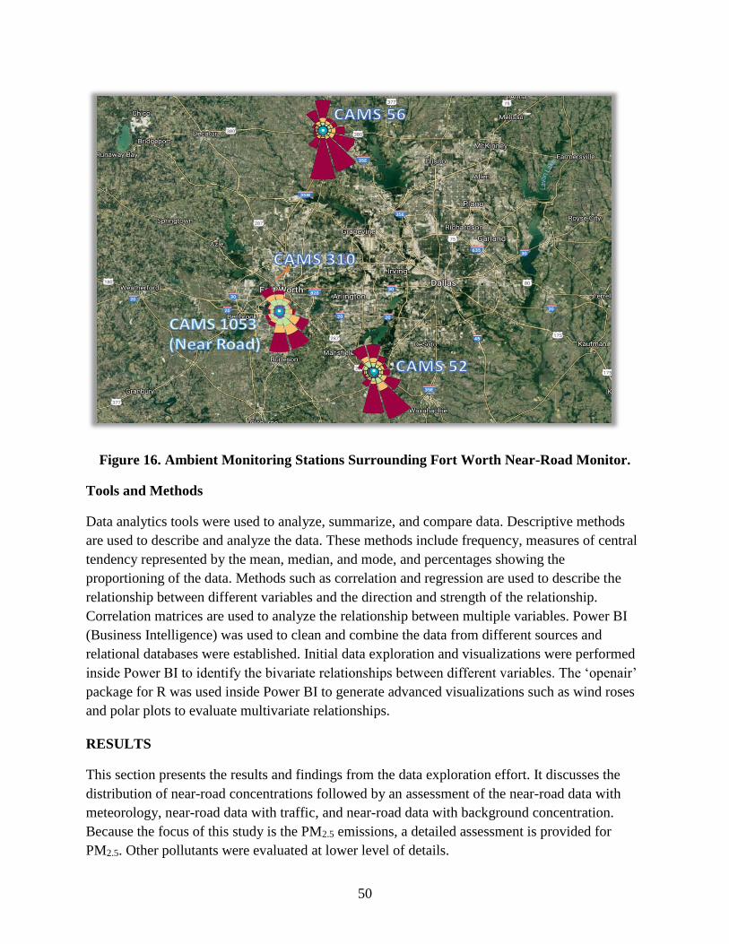
50
Figure 16. Ambient Monitoring Stations Surrounding Fort Worth Near-Road Monitor.
Tools and Methods
Data analytics tools were used to analyze, summarize, and compare data. Descriptive methods
are used to describe and analyze the data. These methods include frequency, measures of central
tendency represented by the mean, median, and mode, and percentages showing the
proportioning of the data. Methods such as correlation and regression are used to describe the
relationship between different variables and the direction and strength of the relationship.
Correlation matrices are used to analyze the relationship between multiple variables. Power BI
(Business Intelligence) was used to clean and combine the data from different sources and
relational databases were established. Initial data exploration and visualizations were performed
inside Power BI to identify the bivariate relationships between different variables. The ‘openair’
package for R was used inside Power BI to generate advanced visualizations such as wind roses
and polar plots to evaluate multivariate relationships.
RESULTS
This section presents the results and findings from the data exploration effort. It discusses the
distribution of near-road concentrations followed by an assessment of the near-road data with
meteorology, near-road data with traffic, and near-road data with background concentration.
Because the focus of this study is the PM2.5 emissions, a detailed assessment is provided for
PM2.5. Other pollutants were evaluated at lower level of details.

51
Distribution of Near-Road Pollutants
The near-road monitoring data were compared with the NAAQS levels. This comparison is for
only research purposes and not meant to assess or verify attainment status as designated by EPA.
The near-road sites investigated in this study do not have sufficient data to determine whether a
NAAQS violation may have occurred. NAAQS calculations require three years of valid
monitoring data.
Figure 17 and Figure 18 show the distribution of NO2, CO, and PM2.5 in the form of a frequency
distribution and box plot where the red dotted lines indicate the NAAQS levels. Based on the
data for 2016, both Houston and Fort Worth site do not appear to have high concentrations at a
frequency enough to violate the NAAQS.
Figure 17. Relative Frequency and Statistics of Air Pollutants Monitored at Houston Site.

52
Figure 18. Relative Frequency and Statistics of Air Pollutants Monitored at Fort Worth
Site.
Near-Road Concentration and Meteorology
Meteorology has a strong impact on the pollutant dispersion. Researchers evaluated the influence
of key meteorological parameters on near-road concentrations. Figure 19 shows the wind rose
plot that represents the frequency of occurrence of wind direction and wind speed categories for
both near-road stations. The predominant wind direction for both stations is from the southwest
to northeast, and both stations are downwind of the highway emissions for more than 50 percent
of the time based on the data collected for 2016.

53
Figure 19. Wind Rose for a) Houston Site; b) Fort Worth Site
Polar concentration plots that present the frequency of occurrence of pollutant concentrations
categorized by wind direction and wind speed for CO, NO2, and PM2.5 are shown in Figure 20
and Figure 21 for Houston and Fort Worth sites, respectively. For the Houston site, high CO
concentrations were observed when the station was downwind of the traffic emissions, with the
highest observed when winds are blowing from the southeast. Ninety-six percent of highest NO2
readings occurred when the station was downwind from the highway and further NO2 peaking
observed during evening peak hours (4–10 p.m.). Compared to CO and NO2, PM2.5 is more
distributed in the southeast and southwest quadrant, which implies there could be other factors
influencing its distribution. Peaking for all the pollutants are found to occur during wind speeds
lower than 5 mph.
For the Fort Worth site, high NO2 and CO concentrations are also observed during low wind
conditions (wind speed lower than 5 mph) and to some extent in the predominant direction as
shown in Figure 21. However, unlike the Houston site, a clear indication of majority of high
concentrations occurring when the station is downwind of highway emissions is not observed
with the Fort Worth site. For PM2.5, peak concentrations are observed in the predominant
southeast direction when the winds are blowing over the highway in contrast to the Houston site,
indicating traffic could be a contributor of PM2.5 at the Fort Worth site.

54
Figure 20. Polar Concentration Roses for Houston Site.

55
Figure 21. Polar Concentration Roses for Fort Worth Site.
Atmospheric stability affects the dispersion of vehicle emissions downwind of the roadways and
is governed by heat and momentum forces in the environment. Atmospheric stability is classified
into unstable (convective conditions), stable (low transport and dispersion), and neutral (in-
between). AERMOD uses a continuous function called Monin-Obukhov length to characterize
atmospheric stability. The three categories of stability represented as a function of the Monin-
Obukhov length are defined as follows:
• Extremely unstable (0 to −100 m).
• Unstable (−100 to −105 m).
• Stable (0 to 105 m), and neutral (greater than 105 m).
CO NO2
PM2.5

56
Figure 22 shows the hourly distribution of atmospheric stability classes for the Houston site. The
near-road PM2.5 concentration trends that were monitored for the highest 10 days in 2016 were
compared to the corresponding trends of the hourly BC and atmospheric stability conditions as
shown in Figure 23. This trend comparison suggests that although high concentration levels seem
to correspond with stable conditions, a clear trend is not observed between the parameters.
Figure 22. Distribution of Atmospheric Stability Classes for Houston Site.
Figure 23. Variation of Houston Near-Road PM2.5 with Atmospheric Stability and
Background Concentration.
Near-Road Concentration and Traffic Activity
The near-road PM2.5 concentrations are evaluated against AADT, FE-AADT, and number of
trucks as shown in Figure 24. High PM2.5 concentration values (i.e., greater than 15 ug/m3) are
observed when AADT value is about 200,000 or FE-AADT is 300,000 (corresponding to 12,000
truck AADT). The very low R2 obtained from linear regression plots indicate a weak correlation
between near-road PM2.5 and traffic metrics. A similar trend was observed for Fort Worth site
with a low R2 value and high PM2.5 concentrations at AADT above 100,000 vehicles as shown in
Figure 25. Due to the lack of data on vehicle classification, variation of the near-road
concentrations at Fort Worth site is presented only for AADT.
Atmospheric Stability

57
Figure 24. Variation of Near-Road PM2.5 with Traffic Activity for Houston Site.

58
Figure 25. Variation of Near-Road PM2.5 with Traffic Activity for Fort Worth Site.
A very slight increase in R2 is found when the near-road increment is combined with AADT
(Figure 26), which indicates a minor influence of traffic activity on the near-road measurements
for the Houston site. But no such increase in R2 is noted for the Fort Worth site. The traffic
counter is located relatively far from the near-road monitor.
Figure 26. Variation of Near-Road PM2.5 Increment with Traffic Activity for Houston Site.
As seen in both Figure 25 and Figure 26, data points are found to cluster around AADT of
around 200,000 indicating a low day-to-day variation level of traffic activity. The weak
correlation presented here is consistent with the findings from DeWinter et al. [51].
y = 2E-05x + 5.8602R² = 0.0313
0
5
10
15
20
0 20000 40000 60000 80000 100000 120000 140000
PM
2.5
Co
nce
ntr
atio
n (
ug/
m3
)
AADT
PM2.5 >15 µg/m3

59
Evaluation of traffic speed is performed only for the Houston site due to the lack of speed data
for Fort Worth site. Figure 27 shows variation of near-road PM2.5 and near-road increment PM2.5
with traffic speed through concentration roses where the dots with different colors represent
PM2.5 concentrations of varying magnitude, and the quadrants represent the wind direction, and
the circles represent traffic speed obtained from the traffic counter. Similar to the traffic volume,
high PM2.5 values are found to cluster around traffic speed ranging between 50 to 60 mph. The
near-road PM2.5 concentration data used in this study are 24-hour averages. It is expected that a
data set with a higher time resolution (e.g., hourly records) would better explain the potential
effect of influential variables.
Figure 27. Variation of Near-Road and Near-Road Increment PM2.5 with Traffic Speed.
Near-road PM2.5
Near-road Increment

60
Near-Road and Background Concentrations
Figure 28 and Figure 29 compare near-road PM2.5 to that measured at other regional stations for
Houston and Fort Worth sites, respectively. The regional monitoring stations record the PM2.5
concentrations in hourly averaged format. The near-road PM2.5 concentrations are found to
exhibit a strong similarity with various regional CAMS stations with R2 ranging from 0.83 to
0.91. This finding is in line with other studies that found the near-road concentrations to be
dominated by background concentrations.
Figure 30 and Figure 31 show a timeseries of the 24-hour PM2.5 concentrations at near-road
stations and at the hourly data from other regional stations for the same day. The 24-hour
averaged PM2.5 concentrations obtained at both the near-road stations exhibits a strong similarity
to the regional CAMS stations. However, both near-road monitors are found to measure higher
PM2.5 concentrations compared to the surrounding ambient monitoring stations. Researchers
calculated an average near-road increment of 1.98 µg/m3 or 19.39 percent and 0.54 µg/m3 or
6.5 percent for the Houston and Fort Worth sites, respectively. These near-road increments are
comparable with the average near-road increment of 15 percent estimated by DeWinter et al.
[51] and less than 22 percent increment reported by Karner et al. [5].

61
Figure 28. Variation of Near-Road PM2.5 with Background Concentration at Houston Site.

62
Figure 29. Variation of Near-Road PM2.5 with Background Concentration at Fort Worth Site.

63
Figure 30. Comparison of 24-Hour PM2.5 Concentrations at Houston Site to that Measured
at Other Regional Stations.
Figure 31. Comparison of 24-Hour PM2.5 Concentrations at Fort Worth Site to that
Measured at Other Regional Stations.

64
Correlation Matrix
A correlation matrix is developed for near-road PM2.5 concentrations that are categorized by
wind direction categories. The wind direction in the range between 90o–180o and 180o–270o are
classified as downwind and between 0o–90o and 270o–360o are classified as upwind. The matrix
represents the correlation between variables and each cell in the matrix represents the strength of
the correlation.
Figure 32 and Figure 33 show the correlation matrix for PM2.5 against key parameters
categorized by upwind and downwind directions for Houston and Fort Worth sites, respectively.
Unlike CO and NO2 where different parameters are identified as influential under different wind
direction conditions, only background concentration is found to have an impact on PM2.5 in both
wind directions. This indicates a very strong correlation between near-road PM2.5 and regional
background concentrations.

65
Figure 32. Correlation Matrix for PM2.5 for Houston Site.

66
Figure 33. Correlation Matrix for PM2.5 for Fort Worth Site.

67
SUMMARY
A comprehensive analysis was performed to evaluate the near-road monitoring data for key
meteorological, traffic, and background concentration data. Researchers used statistical methods
and data analytics tools to perform data exploration research on near-road concentration data
recorded in 2016 by the Houston and Fort Worth near-road monitoring stations. Key findings
from this chapter are as follows:
• NAAQS: Based on the data collected for 2016, the near-road monitoring stations in
Houston and Fort Worth did not appear to have high concentrations of CO, PM2.5, and
NO2 at a frequency enough to violate the NAAQS.
• Meteorology: Both wind direction and wind speed are found to have an impact on CO
and NO2, with high concentrations occurring during low wind speeds and downwind
conditions (i.e., when the monitor is downwind from the roadway in the southeast
direction). This observation indicates that traffic could be a major factor influencing the
distribution of CO and NO2 concentrations during the downwind conditions. PM2.5 is
more distributed in the southeast and southwest quadrant, which implies there could be
other factors influencing its distribution. A clear association between all pollutant
concentrations and atmospheric stability was not observed.
• Traffic: A very weak correlation was observed between the traffic parameters (AADT,
FE-AADT, truck volume, and traffic speed) and PM2.5 concentrations. However, traffic
parameters are found to have an influence on NO2 and CO concentrations during
downwind conditions.
• Background Concentration: Results showed that the coefficient of determination (R2) to
vary between 0.83 and 0.91 for near-road PM2.5 and background PM2.5 concentrations
monitored at surrounding monitoring stations. The changes in near-road PM2.5
concentrations are found to correlate more with the changes of surrounding background
levels values than by any other parameters. On average, there was a 12.8 percent
(1.32 µg/m3) increment at near-road stations compared to ambient monitoring stations.
The findings obtained in this study are consistent with prior studies that found near-road
PM2.5 concentration to be dominantly influenced by regional background concentration
levels compared to traffic and meteorological parameters.


69
CHAPTER 5:
MODELING APPROACH AND DATA
INTRODUCTION
This section discusses the key modeling components involved in air dispersion modeling. The
models and approaches described here include those used for meeting regulatory requirements
(conformity and NEPA analyses). Figure 34 shows the flow of data in the overall framework
used for modeling.
Figure 34. Flow of Data for Modeling.
Air dispersion modeling of roadway emissions requires several types of input data, including
traffic, emission rates, meteorological, and other project-specific data. Modeling roadways as a
source of emissions for both emissions and air dispersion modeling require traffic data as input.
Major sources of traffic data used for emissions and air dispersion modeling include the federal
Emission Modeling
Local Specific Data Inputs
- Vehicle Age Distribution- Fuel Supply- Meteorology
- I/M Program
Traffic Data Inputs
- Traffic Volume- Fleet Composition- Average Speed
Air Dispersion Modeling
Emission Factors (EFs)
EFs assigned to sources
Meteorological Data
Model Control Parameters
Pollutant Type, Averaging Period,
pollutant properties etc.
Base Imagery Source Characterization
- Source Dimensions
- Dispersion Parameters
Receptor Placement
- Receptor Location
- Height
ResultsConcentration estimates at discrete receptors
Traffic Data Characterization
Data Required
Traffic volume, Speed
Fleet Mix, Roadway type etc.
Data Sources
HPMS, STARS-II, Travel demand model, and
other sources (INRIX, NPMRDS)

70
HPMS database, TxDOT’s STARS-II database, metropolitan area TDM, and traffic from
project-level analysis.
Emission rates required for air dispersion modeling are obtained through emission modeling
using the EPA’s MOVES emission model. The MOVES emission model uses traffic data such as
speed, volume, fleet mix, and other locally specific data related to meteorology, vehicle age
distribution, and fuel parameters, to generate total emissions (in grams) or emission factors
(grams per mile or grams per vehicle) at the roadway link level. The dispersion of the traffic
related emissions in the atmosphere is modeled using CAL3QHCR and AERMOD models. The
source (roadway link) specific emission rates from the MOVES model are passed on to the air
dispersion models and are assigned project-specific dimensions, orientations, and properties to
reflect site conditions.
Site-specific meteorological and land use conditions are incorporated into the air dispersion
models. Based on the implementation of the Gaussian dispersion process, air dispersion models
(CAL3QHCR and AERMOD) estimate pollutant concentrations at discrete receptor locations.
Determination of the regional PM BC is an important step in the PM hot-spot process as the BC
is combined with project specific incremental concentrations to determine the design value and
compliance with the air quality standards [9]. Design value is conceptually defined as the sum of
the modeled representative concentration resulted from the project and the background
concentration. The project-specific contribution is estimated using MOVES emission and
AERMOD air dispersion modeling [9]. BC is estimated using concentrations measured by
surrounding ambient monitoring stations. Statistical and GIS tools are used for data analyses of
the modeled estimates. This chapter describes the different modeling components and their
corresponding data requirements and sources.
TRAFFIC ACTIVITY DATA
Researchers examined the available traffic data for the study areas. The team determined that the
traffic activity data were not available for all the links in the study areas, so they used outputs of
regional TDM for both case study sites. TDM network for the 12-county DFW area was
provided by the North Central Texas Council of Governments (NCTCOG). Similarly, the 8-
county TDM outputs for Houston Galveston area was provided by Houston Galveston Area
Council (HGAC). The TDM outputs were provided for AM peak, PM Peak, Off Peak, and night
time. The links were processed to estimate hourly traffic outputs using TTI TDM link-based
method [84]. The roadway network links and associated traffic data (volume, speed) close to the
Houston and Fort Worth near-road monitoring sites were extracted as shown in Figure 35 and
Figure 36 and further processed for dispersion modeling analysis.

71
Figure 35. Roadway Network Links Extracted from TDM for Fort Worth.
Figure 36. Roadway Network Links Extracted from TDM for Houston.
TDM outputs extracted correspond to the traffic volume and traffic speed. Following PM hotspot
analysis guidelines for a worst-case scenario, maximum hourly traffic volume in each of four
daily time periods (morning peak [6–9 a.m.], midday [9 a.m.–4 p.m.], evening peak [4–7 p.m.],
and overnight [7 p.m.–6 a.m.]) and for corresponding volume weighted average speed for each
time period (four periods) were obtained and used in emission estimation process.
MOVES MODELING
Emission rates required for air dispersion modeling are obtained through emission modeling
using the EPA’s MOVES (MOVES2014a) emission model. MOVES requires information for

72
vehicle types, ages, fuel types, and the emissions parameters to estimate emission rates.
Researchers used the latest MOVES2014a inputs in combination with TTI’s State
Implementation Plan-quality inventory development methodology, designed for use with
MOVES. MOVES RunSpecs or MRS provides instructions for how and what data to be used for
estimating emission rates. Table 5 provides the RunSpecs information used for estimating
emission rates that were used in this study. One RunSpec and one county database per area are
required for each MOVES run. Each RunSpec was designed to produce a separate,
corresponding MOVES output database (i.e., one output database per run). There were 64 MRS
input files and 64 county databases, and correspondingly 64 MOVES input and output databases,
produced under this task.
Table 5. Input Parameters for MOVES2014a Runs.
Input Item Description
Run Specification
Scale Project Scale
Calculation Type Emission Rate
Geographic Bounds Tarrant County, Harris County TX
Time Period Analysis Years: 2016
Seasons: Summer (July), Fall (Oct), Spring (April),
Winter (Jan)
Time-of-day: AM Peak (6–9 a.m.), PM Peak (4–7 p.m.),
Midday (9 a.m.–4 p.m.), and Overnight (8 p.m.–6 a.m.)
Road Type Rural and Urban Restricted and Unrestricted Access
Vehicle Type All
Pollutant Type PM2.5
Emission Process Running Exhaust, Crankcase Running Exhaust, Brake
and Tire Wear
Project Data Manager (Project Specific Input Data)
Link Length One mile
Average Speed Ranging from 2.5 mph to 75 mph at 1 mph increment
Additionally, re-suspended dust emissions factors from paved roads (i.e., TDM roadway links)
were developed according to Equation 2 in AP-42 section 13.2.1 [85]. Finally, MOVES
composite emission factors are combined with re-suspended emission rates for each link for each
time period and season to be processed under dispersion modeling tools.

73
AIR DISPERSION MODELING
In this study both AERMOD and CALINE 3 were used to model two urban sites at Houston and
Fort Worth, Texas. Figure 37 shows the dispersion modeling process, which consists of three
steps, as described below.
Figure 37. Air Dispersion Modeling.
Step 1
This step consists of assembling the base imagery, processing meteorological and land use
conditions specific to the case study site, and specifying model control parameters.
Base Imagery
Base imagery of the case study site is obtained from Google Earth. The base imagery helps with
placing and geographically coding the sources and receptors.
Meteorological and Land Use Data
Meteorological and land use conditions are a major factor that affects pollutant dispersion in the
atmosphere. Three types of data are required for processing the meteorological data, namely:
• Surface data that measure characteristics of lower layers of the atmosphere.
• Upper air data that measure characteristics that change with height in the atmosphere
(such as temperature).
• Land use data that represent surface characteristics.
According to the EPA’s Guideline on Air Quality Models (40 CFR Appendix W to Part 51), “the
meteorological data used as input to an air quality model should be selected on the basis of
spatial and climatological (temporal) representativeness as well as the ability of the individual

74
parameters selected to characterize the transport and dispersion conditions in the area of
concern” [3]. The use of 5 years of adequately representative (off-site) NWS meteorological data
or at least 1 year of site-specific meteorological data is required. As part of Task 3, the team
developed the meteorological inputs using both methods for the case study sites (i.e., the five
consecutive years [2012–2016] of off-site meteorological data using nearby NWS airport data
and the two years [2015–2016] of on-site meteorological data using site-specific data).
The raw data are processed using meteorological preprocessors to produce data in a format
compatible for AERMOD, and CAL3QHCR. Preprocessors used for AERMOD correspond to
AERMINUTE, AERSURFACE and AERMET, and MIXGHT and PCRAMMET for
CAL3QHCR. Process of generating model compatible meteorological data is provided in
Appendix A.
Specific to the AERMOD model, TCEQ produces pre-processed AERMOD-compatible off-site
meteorological data for all counties in the state of Texas. For each county, TCEQ produces three
sets of meteorological data corresponding to three categories of surface roughness (low, medium,
and high). Based on the surface roughness obtained through processing of case study site-
specific land use data, appropriate meteorological data were recommended to be used. Surface
roughness values ranging from 0.001 m to 0.1 m represent the low surface roughness category,
values ranging from 0.1 m to 0.7 m represent medium surface roughness. and high surface
roughness category represent surface roughness length values ranging from 0.7 to 1.5 m [70].
Model Control Parameters
In addition to assembling data corresponding to emissions, meteorology, and land use, the first
step also consists of defining the model control parameters for the air dispersion model.
General Parameters
The model control parameters are used to specify the pollutant type (PM2.5), pollutant properties
(no deposition and settling), and averaging period (hourly, 24-hours and annual) for which the
concentration estimates are modeled.
Urban Heat Island Effect
The land use designation in air dispersion models is represented in two ways:
• Use of meteorological data from a representative urban/rural site.
• Use of dispersion option for indicating use of urban heat island.
For urban areas, the model activates the urban heat effect, a term used to describe urban areas
that are hotter than nearby rural areas, especially at night, mainly because of heat retention by
urban materials. Because of this heat retention, the vertical motion of the air is increased through

75
convection, thereby leading to the increased dispersion of pollutants [86]. CAL3QHCR allows
the user to prompt the urban heat island effect by specifying U for urban and R for rural land use
in the input file. AERMOD accounts for urban dispersion effects by activating a switch as on for
urban and off for rural areas and also requires the urban area population to determine the degree
of urban heat island effect occurring in a specific urban area.
Step 2
This step involves characterizing the emission sources (i.e., adjacent roadway links), processing
emission factors in a format compatible for air dispersion modeling and placing receptors.
Source Characterization
AERMOD can model roadway line source as a series of volume or area sources. CAL3QCHR
models roadway links only as line sources. Sources in both models are defined based on the:
• Travel activity that corresponds to volume and speed.
• Physical dimensions.
• Orientation.
For example, a single source can be used for a roadway link if the entire link has the same travel
activity and no change in geometry. However, for a curved link with the same travel activity,
more than one source is required to be used to preserve the geometry. The BREEZE AERMOD
and BREEZE ROADS models, commercial propriety software developed by Trinity Consultants
Inc., which provides an unaltered, user-friendly, window-based version of the EPA-approved
AERMOD model with pre- and post-processors, is used to help with the source and receptor
coding with AERMOD and CAL3QHCR, respectively.
Dispersion Parameters
The following dispersion parameters are used in AERMOD air dispersion modeling, based on
the methodology specified in the EPA guidance [9]:
─ Initial Vertical Dispersion Coefficient
According to EPA hot-spot guidance [13], the initial vertical dispersion dimension is
assumed to be about 1.7 times the average vehicle height, to account for the effects of
vehicle-induced turbulence. For light-duty vehicles, this height is about 2.6 m, using an
average vehicle height of 1.53 m, or 5 ft. For heavy-duty vehicles, this height is about
6.8 m, using an average vehicle height of 4.0 m. The AERMOD User’s Guide
recommends that the initial vertical dispersion coefficient (σzo) to be estimated for a
surface-based area/volume source by dividing the initial vertical dimension by 2.15. For
typical light-duty vehicles, this figure corresponds to a σzo of 1.2 m. For typical heavy-
duty vehicles, this figure corresponds to a σzo of 3.2 m. For roadway links having a

76
combination of light-duty and heavy-duty traffic, the guidance recommends the
coefficient to be calculated as a combination of their respective σzo values by using a
traffic volume-weighted or emissions-weighted average.
─ Source Release Height
Source release height is the height at which wind effectively begins to affect the plume
and is estimated from the midpoint of the initial vertical dimension. For moving light-
duty vehicles, this is about 1.3 m. For moving heavy-duty vehicles, it is 3.4 m. Similar to
σzo, the source release height for roadways with a combination of light duty and heavy-
duty vehicles is calculated using a traffic volume-weighted or emissions-weighted
average.
─ Emission Rates from MOVES
Characterization of emission sources consists of defining their dimensions and
designating the rate at which the source produces emissions. Emission rates obtained
from MOVES are converted into a format compatible for the air dispersion model and the
source type used. AERMOD requires a composite ER (in grams/sec/m2) for the area
source approach and ER (in grams/sec) for volume source approach. CAL3QCHR
requires ER in form of grams/vehicle-mile.
─ Receptor Placement
Receptors are locations in the study area where an air dispersion model estimates
pollutant concentration. As per the EPA guidance, receptors should be located throughout
the study area in publicly accessible areas where high PM concentrations would be
expected. Receptor spacing near the source (roadways) should be of sufficient resolution
to capture the concentration gradient around the locations of maximum-modeled
concentrations. Receptors are placed at a height of 1.8 m above the ground. For
evaluating modeling results with the near-road data, receptors are placed at the near-road
monitoring location for both study sites. In addition, concentration contour maps are
generated by placing grid receptors at varying spacing from the roadway links.
Step 3
This step consists of multiple runs of the air dispersion models using files prepared in Steps 1
and 2. Model outputs include pollutant concentration estimates at different averaging time
period. The annual average concentrations presented in this study are all-period averages of non-
zero hourly concentrations.
BACKGROUND CONCENTRATION
Background air quality includes pollutant concentrations occurring due to area-wide or regional
sources. The EPA’s guidance on hot-spot analysis states that BC should be as representative as
possible for the area where the project site is located. Ideal BC for a near-road site without the
influence of traffic emissions are rarely available. For an area surrounded by multiple
background ambient PM2.5 monitors, EPA recommended that the data should be analyzed by

77
statistical or mapping methods to develop a BC for use in the hot-spot analysis. Four methods,
based on either a single station or multiple stations, are recommended by EPA for developing the
BC. However, no specific guidance was provided on which method is preferred for an area.
In this study, researchers used seven methods to estimate BC for the case study sites. Four of the
methods are suggested by EPA for BC estimation. The data used in this analysis were obtained
from onsite weather station at the near-road monitoring location and multiple urban-scale
stations surrounding the two case study sites. Statistical analyses and performance of each
method were compared to determine the best approach for BC estimation. To test the methods,
one station is designated as the target station and its data were treated as observations while the
data from other stations were used to developed background concentration estimates. In other
words, the PM2.5 concentration, 𝑥𝑖,𝑗, represents a concentration observed at station i and at a time
step j.
xi,j = PM2.5 concentrations, i = 1, …, m and j = 1, …, n
where
m: Number of stations
n: Number of data records
The methods are described as follows.
Method 1: Single Station Estimate
𝑦𝑖,𝑗𝑠 = 𝑥𝑘,𝑗 (𝑘 ≠ 𝑖) (4)
The single station approach looks for a station that best represents the background concentration
for the project site. Factors to be considered in selecting the best representative background site
for the project site include distance to the project area, located upwind and similarity in terms of
land use, meteorological, and mix of sources. Surface or boundary layer parameters such as
surface albedo, Bowen ratio, and roughness for the sites were obtained from the National Land
Cover Dataset and processed using the AERSURFACE model. The surface characteristics within
5 km of all site were judged to be very similar. A close look of the land use distribution indicates
that most of the sites can be described as residential communities of high and low intensity
combined with moderate commercial, industrial, and transportation facilities. Without a clear
distinction in the topologic and meteorological conditions among these sites, the most
representative single station was selected based only on the shortest distance to the project site.
Method 2: Arithmetic Mean
The arithmetic mean approach provides an estimate by taking the average of concurrent data
from all available background sites:

78
𝑦𝑖,𝑗 = 1
𝑚−1[( ∑ 𝑥𝑘,𝑗
𝑚𝑘=1 ) − 𝑥𝑖,𝑗] (5)
Method 3: Weighted Mean Estimate by Inverse Distance
This method provides an average weighted by the inverse of the distance to the study site. The
distance matrix is defined as 𝐷𝑖𝑠𝑡𝑎𝑛𝑐𝑒𝑖,𝑘 = 𝐷𝑖𝑠𝑡𝑎𝑛𝑐𝑒 𝑏𝑒𝑡𝑤𝑒𝑒𝑛 𝑠𝑡𝑎𝑡𝑖𝑜𝑛 𝑖 𝑎𝑛𝑑 𝑘 and the
weighting factor Weight1i,k is:
𝑊𝑒𝑖𝑔ℎ𝑡1𝑖,𝑘 =
1
𝐷𝑖𝑠𝑡𝑎𝑛𝑐𝑒𝑖,𝑘
∑1
𝐷𝑖𝑠𝑡𝑎𝑛𝑐𝑒𝑖,𝑘
𝑚𝑘=1𝑘≠𝑖
, 𝑘 ≠ 𝑖 (6)
and 𝑊𝑒𝑖𝑔ℎ𝑡1𝑖,𝑘 = 0, 𝑖𝑓 𝑘 = 𝑖
The estimate zi,j is obtained as:
𝑧𝑖,𝑗 = ∑ (𝑥𝑘,𝑗 ∙𝑚𝑘=1 𝑊𝑒𝑖𝑔ℎ𝑡1𝑖,𝑘) (7)
Method 4: Weighted Mean by Inverse Distance Squared
This method is similar to Method 3 except the weighting factor is represented by the inverse of
the distance to the square. The weighting factor Weight2i,k is defined as:
𝑊𝑒𝑖𝑔ℎ𝑡2𝑖,𝑘 =
1
(𝐷𝑖𝑠𝑡𝑎𝑛𝑐𝑒𝑖,𝑘)2
∑1
(𝐷𝑖𝑠𝑡𝑎𝑛𝑐𝑒𝑖,𝑘)2𝑚𝑘=1𝑘≠𝑖
, 𝑘 ≠ 𝑖 (8)
and 𝑊𝑒𝑖𝑔ℎ𝑡2𝑖,𝑘 = 0, 𝑖𝑓 𝑘 = 𝑖
The estimate wi,j is:
𝑤𝑖,𝑗 = ∑ (𝑥𝑘,𝑗 ∙𝑚𝑘=1 𝑊𝑒𝑖𝑔ℎ𝑡2𝑖,𝑘) (9)
Method 5: Normalized Arithmetic Mean Estimate
This method seeks to preserve the trend of the time series data at each station by normalizing the
time series data at each station by its own annual average. The normalized data Xi,j becomes:
𝑋𝑖,𝑗 =𝑥𝑖,𝑗
1
𝑛∑ 𝑥𝑖,𝑗
𝑛𝑗=1
, 𝑖 = 1, ⋯ , 𝑚, 𝑗 = 1, ⋯ , 𝑛 (10)
The normalized estimate becomes Yi,j and the estimate can be retrieved by multiplying Yi,j by
the annual average of yi,j:
𝑌𝑖,𝑗 = 1
𝑚−1[( ∑ 𝑋𝑘,𝑗
𝑚𝑘=1 ) − 𝑋𝑖,𝑗] (11)

79
𝑦𝑖,𝑗𝑁 = 𝑌𝑖,𝑗 ∙ (
1
𝑛∙ ∑ 𝑦𝑖,𝑗
𝑛1 ) (12)
Method 6: Normalized Inverse Distance Estimate
Similar to Method 5, the normalized inverse distance estimate is Zi,j and the estimate can be
retrieved by multiplying Zi,j by the annual average of yi,j:
𝑍𝑖,𝑗 = ∑ (𝑋𝑘,𝑗 ∙𝑚𝑘=1 𝑊𝑒𝑖𝑔ℎ𝑡1𝑖,𝑘) (13)
𝑧𝑖,𝑗𝑁 = 𝑍𝑖,𝑗 ∙ (
1
𝑛∙ ∑ 𝑧𝑖,𝑗
𝑛1 ) (14)
Method 7: Normalized Inverse Distance Squared Estimate
The normalized inverse distance squared estimate Wi,j and the estimate wi,j is:
𝑊𝑖,𝑗 = ∑ (𝑋𝑘,𝑗 ∙𝑚𝑘=1 𝑊𝑒𝑖𝑔ℎ𝑡2𝑖,𝑘) (15)
𝑤𝑖,𝑗𝑁 = 𝑊𝑖,𝑗 ∙ (
1
𝑛∙ ∑ 𝑤𝑖,𝑗
𝑛1 ) (16)
Appendix B presents detailed discussions of the methodology.
OTHER TOOLS AND METHODS
Data analytics tools were used to analyze, summarize, and compare data. Descriptive methods
are used to describe and analyze the data. These methods include frequency, measures of central
tendency represented by the mean, median, and mode, and percentages showing the
proportioning of the data. Methods such as correlation and regression are used to describe the
relationship between different variables as well as the direction and strength of the relationship.
Correlation matrices are used to analyze the relationship between multiple variables. Power BI
(Business Intelligence) was used to clean and combine the data from different sources and
relational databases were established. Initial data exploration and visualizations were performed
inside Power BI to identify the bivariate relationships between different variables. The ‘openair’
package for R was used inside Power BI to generate advanced visualizations such as wind roses
and polar plots to evaluate multivariate relationships.
Over the recent year, the availability of GIS data has increased both in quantity and quality.
Moreover, the realization of easy-to-use GIS software and GIS tools has made application of
GIS-based decision support tools more practical. ArcGIS has been one of the most population
software widely used for GIS applications and will be used for this project. ArcGIS will be used
to create the maps used in the near-road monitoring siting, case study site selection process,
characterization of traffic data, selection of suitable meteorological stations, etc. Table 6 shows

80
the GIS data inputs and data sources for this project. Numerous map layers are created, and the
near-road monitoring site selection criteria were applied to select the near-road monitoring sites
for the model-to-monitor evaluation. Traffic data from different sources and other spatial data
related to roadway network and topography are combined with the near-road monitoring
locations to decide the appropriate traffic data source for characterizing traffic near the near-road
monitoring station. Location of surface and upper air stations are combined with the near-road
monitoring stations to select the appropriate stations for obtaining meteorological data specific to
the case study site. In addition to these applications, GIS will be also be used in form of base
imagery to help with the coding of emission sources and receptors.
Table 6. GIS Data Inputs and Sources.
Data Input Source Comments
Traffic Data TxDOT Traffic Counts, AADT, RHiNo, STARS, etc.
MPO and Local
Governments
Local Traffic Counts, TDM
Other Data Sources INRIX, NPMRDS, Google, etc.
Road Network
TxDOT Current and Future
MPO Current and Future
Topography TCEQ Geocoded based on X and Y coordinates obtained
from TCEQ
https://www.tceq.texas.gov/airquality/monops/site
s/air-mon-sites
Near-road Monitoring
Station Locations
Google Earth https://www.google.com/earth/
TCEQ Air monitoring location and parameters collected
Pollutant
Concentration
TCEQ/EPA https://www.tceq.texas.gov/airquality/monops/site
s/air-mon-sites
Aerial Imagery Google Earth https://www.google.com/earth/
Presence of other air
pollution sources,
water bodies and
points of interest
Land Use (U.S. Geological
Survey)
https://www.usgs.gov/
Meteorology TCEQ https://www.tceq.texas.gov/permitting/air/nav/dat
asets.html
NCDC https://www.ncdc.noaa.gov/data-access/land-
based-station-data/land-based-datasets/automated-
surface-observing-system-asos

81
SUMMARY
This chapter overviews the different modeling components involved in the PM hot-spot
modeling process. Track 2 of this research project is focusing on evaluating key modeling
parameters within each of these modeling components. The following chapters overview the
different modeling scenarios and the results obtained.


83
CHAPTER 6:
MODELING SCENARIOS AND RESULTS
INTRODUCTION
Task 3 of this research project focused on evaluating the air dispersion modeling process of PM
hot-spot analysis. Researchers used a series of sensitivity analyses to investigate the variabilities
in AERMOD and CAL3QHC models’ outputs in the context of regulatory PM hot-spot analysis.
The modeling components included in the sensitivity analyses correspond to traffic activity,
emissions estimation, air dispersion modeling, meteorology information, and background
concentration as described in Chapter 5. As part of the sensitivity analysis, researchers set-up a
baseline case (“baseline”) that corresponds to the regulatory PM hot-spot analysis process (i.e.,
all parameters are defined according to the PM hot-spot analysis requirements). Alternative
scenarios are set-up based on alternative methods and values corresponding to each of the key
modeling components. The sensitivity analysis was performed for the Fort Worth and Houston
near-road monitoring stations measuring. This chapter describes the different modeling scenarios
developed and the results obtained for both the case study sites.
MODELING SCENARIOS
Researchers developed different modeling scenarios corresponding to the key modeling
components involved with the PM hot-spot process. The modeling components correspond to
traffic activity characterization, emission modeling, air dispersion modeling, meteorological
data, and background concentration. The different input parameters evaluated correspond to
those parameters that are ambiguous or not clearly defined to state agencies or practitioners when
implementing the hot-spot modeling process following the EPA guidance. These scenarios are
discussed in this section.
Traffic Data Characterization
EPA recommends a minimum of 16 MOVES runs necessary for a PM hot-spot modeling to
capture changes in emission rate due to changes in ambient conditions [87]. These 16 models
runs correspond to four weekday time periods as morning peak AM (6–9 a.m.), midday MD (9
a.m.–4 p.m.), evening peak PM (4–7 p.m.), and overnight ON ( 7 p.m.–6 a.m.) for four
representative months as January (winter season), April (spring), July (summer), and October
(fall). To account for the worst-case scenario, the peak-hour traffic in each period was used as a
constant rate for all the hours in the corresponding period. Results from each of the four hours
from four periods were extrapolated to cover the entire day and the results of these 16 model
runs were extrapolated to cover the whole year. To test the sensitivity of the traffic data, three
scenarios were considered:

84
• Baseline Scenario: Use the peak-hour traffic for four time periods.
• Scenario 1: Use average hour traffic for four time periods.
• Scenario 2: Use hourly traffic for 24 hours.
Emission Modeling
For MOVES emission analysis, EPA guidance recommends using inputs consistent with inputs
used for regional emission analysis. These inputs correspond to meteorology, fuel supply, and
age distribution. Alternative scenarios were set up to evaluate the difference based on local case
study specific MOVES inputs:
• Baseline Scenario: MOVES inputs consistent with inputs used for regional emission
analysis.
• Scenario 3: Case-study specific input corresponding to meteorological (temperature and
humidity) data obtained from near-road onsite parameters.
Meteorological Data Processing
Onsite versus Offsite Meteorological Data
For PM hot-spot analysis, EPA recommends using either one year of onsite meteorological data
or five years of latest available offsite meteorological. Specific to Texas, TCEQ produces
AERMET processed meteorological data for three sets of surface roughness. Depending on the
site-specific surface roughness (SR), the appropriate data are used. Researchers selected the
following scenarios:
• Baseline Scenario: On year of onsite meteorological data.
• Scenario 4: Five years of offsite meteorological data corresponding to offsite low surface
roughness.
• Scenario 5: Five years of offsite meteorological data corresponding to offsite medium
surface roughness.
• Scenario 6: Five years of offsite meteorological data corresponding to offsite high surface
roughness.
Land Use Designation
Guidelines on deciding the urban/rural representativeness of a source are given in [88], in which
a land use classification or population density method should be employed. In most cases the
first approach may suffice. If not, the latter approach may be taken. In reality, a project site may
be situated in an area that is ambiguous to either definition above. In that case, a different
designation of the project site will affect the model results. The question is by how much. To
evaluate the effect of an incorrect land use designation, the team developed Scenario 7 to
evaluate the impact of land use designation of a modeling site on the near-road PM2.5

85
concentration levels—Scenario 7: Land use designation was changed from urban to rural while
traffic parameters and site geometry were unchanged.
Air Dispersion Modeling
Source Type
EPA guidance recommends modeling roadway links as area or volume sources for PM hot-spot
analysis. Table 7 lists the difference between the two sources.
Table 7. Difference between Area and Volume Sources in AERMOD.
Area Source in AERMOD Volume Source in AERMOD
Definition Area sources are flat, two-dimensional
spaces from which emissions originate.
They are more appropriate for near
ground level sources with no plume rise
(viaduct, storage piles).
Volume sources are three-dimensional
spaces from which emissions originate.
They are more appropriate for line sources,
which have some initial plume depth (rail
lines, conveyor belts).
Algorithm Area sources models emissions with a
uniform distribution across the roadway
link and are not distributed beyond the
edge of a roadway link.
Area sources does not incorporate the
plume meander algorithm that accounts
for the laternal back-and-forth shifting
of an emission plume under low wind
conditions.
Volume sources model emissions with a
Gaussian distribution, that represents a
decrease in emission density, both
horizontally and vertically as the distance
from the roadway increases.
Volume sources incorporates the plume
meander algorithm.
Exclusion
Zone
Area sources does not have the
exclusion zone and can calculate
concentrations at receptors within the
source.
Volume sources have an exclusion zone
where concentrations are not calculation,
in other words if a receptor is located in the
exclusion zone, volume source will not
calculate any concentrations at that
receptor. Exclusion zone is the region
((2.15 × Sigma Y) + 1 meter)) from the
center of the volume.
Runtime A fewer number of area sources are
required to represent a given roadway
link compared to volume source as
shown in Figure 38.
More volume sources are required to
represent a given roadway link compared
to area sources. Because of a larger
number of sources required to characterize
a given link, processing times are longer
both in terms of model set-up and run time.

86
Figure 38. Area and Volume Source Representation of a Roadway Link.
Scenario 8 was designed to evaluate the differences in concentration estimates using area and
volume source characterization—Scenario 8: roadway links were characterized as volume
sources.
Model Comparison
Comparison was made to evaluate the variation in outputs between CAL3QHCR and AERMOD:
• Scenario 9: CAL3QHCR was used to estimate the near-road concentrations. Input
parameters were consistent with AERMOD baseline (Baseline Scenario).
• Scenario 10: this scenario was set up to evaluate CAL3QHCR with offsite meteorological
data.
Based on these parameters listed above different scenarios were developed as shown in the Table
8.
Background Concentration
For both case study sites, the annual average PM2.5 concentrations developed from different
methods (described in Chapter 5 and Appendix B) are evaluated using different performance
metrics. These metrics used in this study are described below:
• Normalized Mean Bias (NMB) is a measure of the average deviation from actual
observation (between −1 and ∞). The NMB represents the average model bias normalized
by the mean of observations, with considering (positive and negative) direction of the
errors.
• Normalized Mean Error (NME) is a measure of the averaged absolute deviation without
considering direction of differences between prediction and observation (between 0 and
∞). Contrary to the NMB, in the NME the absolute deviations are summed instead of the
differences, and we have equal weight of underestimation and overestimation.
Roadway Link

87
• Normalized Root Mean Square Error (NRMSE) is a measure of the square root of the
average of the squared differences between prediction and actual observation (between 0
and ∞). The root mean squared error (RMSE) represents standard deviation of the
differences between predicted and observed values. In RMSE, the squared differences are
averaged, and the measure gives a relatively high weight to large errors compared with
the mean error.
In practice, the statistics are based on finite samples of several sets of concentrations, and do not
represent sampling variability. Researchers used a statistical technique known as bootstrapping
to account for the sampling variability in the predictions [89]. The bootstrap is a resampling
method to estimate standard error of a specific performance measure computed from resampled
dataset. The bootstrap procedure follows the basic steps:
1) Resample a given data set a specified number of times. In other words, generate new
estimates 𝑥𝑖,𝑗(1)
, 𝑥𝑖,𝑗(2)
, ⋯ , 𝑥𝑖,𝑗(𝐵)
where B is the bootstrap sample size (e.g., B=5,000).
2) Calculate a specific statistic from each sample (i.e., calculate 5,000 sets of the estimates
for each method). For example, generate 𝑦𝑖,𝑗(1)
, 𝑦𝑖,𝑗(2)
, ⋯ , 𝑦𝑖,𝑗(𝐵)
and calculate 5,000 sets of
NRMSE based on the prediction using inverse distance.
3) Find the standard deviation of the distribution of that statistic. Bootstrapped standard
deviations are obtained to compare sampling variabilities of the statistic (i.e., NRMSE)
between the seven methods.
For both case study sites, the annual average PM2.5 concentrations developed from different
methods were found, in general, acceptable except the single station approach that is selected
based on shortest distance to a target station. Normalized methods appear to perform better than
non-normalized methods with higher accuracy. Among the normalized methods, predictions
made by normalized inverse distance squared method appear to be slightly better than other
models, based on the statistical metrics for annual, 24-hr, and highest 10 24-hr average PM2.5
concentrations.
MODEL SET-UP
Table 8 shows the modeling scenarios developed for both case study sites. Table 9 and Table 10
list the modeling parameters used for the Fort Worth and Houston sites, respectively. Figure 39
and Figure 40 show the model set-up for the Fort Worth and Houston sites, respectively.

88
Table 8. Scenario Development.
Scenario Model Traffic Emissions Meteorology
Dispersion
Parameters Notes
Baseline AERMOD Maximum Regulatory
MOVES inputs Onsite (1 year) Area Baseline for all runs
Scenario 1 AERMOD Average Regulatory Onsite Area Effect of using
different traffic inputs Scenario 2 AERMOD Hourly Regulatory Onsite Area
Scenario 3 AERMOD Maximum Onsite MOVES
Inputs Onsite Area
Effect of using
different inputs for
emission estimation
Scenario 4 AERMOD Maximum Regulatory Offsite (5 years)
(Low SR) Area
Effect of using
different
meteorological data
for dispersion
modeling
Scenario 5 AERMOD Maximum Regulatory Offsite (Med SR) Area
Scenario 6 AERMOD Maximum Regulatory Offsite (High SR) Area
Scenario 7 AERMOD Maximum Regulatory Onsite Area, Rural Effect of urban heat
island effect
Scenario 8 AERMOD Maximum Regulatory Onsite Volume
Effect of different
source type in
AERMOD
Scenario 9 CAL3QHCR Maximum Regulatory Onsite (1 year) Line Effect of different
meteorological data
with different
dispersion model Scenario 10 CAL3QHCR Maximum Regulatory Offsite (5 years) Line
*SR: Surface Roughness

89
Figure 39. AERMOD Area Source and Receptor Placement for Fort Worth.
(a) Fort Worth

90
Figure 40. AERMOD Area Source and Receptor Placement for Houston Site.
(b) Houston

91
Table 9. Input Data Parameters for Fort Worth Site.
Modeling
Parameters Inputs
Base Imagery − Google Earth image covering the case study extent
Model Control
Parameters
− Pollutant: PM2.5
− Averaging Period: 24 hours and annual
− Pollutant Properties: No deposition and settling
− CONC: Specifies that concentration values will be calculated
− FLAT: Specifies that the terrain is flat
Meteorology
− Offsite pre-processed meteorological data consisting of surface, upper air and
land use data representative of case study location is obtained from TCEQ for
five years (2012 to 2016)
− A year (2016) of raw surface data is obtained from Fort Worth Meacham Airport,
upper air data at Fort Worth, and site-specific meteorological parameters (such as
dry bulb temperature, wind direction, and wind speed) are obtained from the Fort
Worth near-road monitoring station
Source
Characterization
− Sources are defined based on (1) travel activity (2) physical dimensions and (3)
orientation
− AERMOD Area source: case study site was modeled with a total of 59 area
sources
− AERMOD Volume source: case study site was modeled with a total of 2606
volume sources
− CAL3QHCR Line source: case study was modeled with 57-line sources
Emission Factor
− ERs from MOVES
− ERs are normalized with reference to time, and source properties (dimensions,
volume) to produce ERs in grams/sec/m2 for area source and grams/second for
volume source approach in AERMOD, grams/vehicle-mile for line source
approach in CAL3QHCR
− EMISFACT-HROFDY: This option is to specify a variable emission rate for the
sources. The rates vary by the hour of the day
Dispersion
Parameters
− Source release height was set at 1.487 m and an initial vertical dispersion of
1.384 m were used
− URBANOPT: Sources are modeled as urban to account for the urban heat island
effect
− Urban roughness length of 1 m is used, and MSA population of 6,426,214 for
AERMOD. For CAL3QHCR modeling, surface roughness was set to 0.01 m as
the default value
Receptor
Characterization
− Receptors positioned at a height of 1.8 m, are placed at the near-road monitoring
station for sensitivity analysis
− For contour plot showing the spatial concentration distribution, grid receptors are
placed starting at 5 m–50 m at a spacing of 15 m, 50 m–200 m at a spacing of
50 m, and 100 m–500 m at 100 m spacing resulting in a total of 1,272 receptors
Output − PM2.5 estimates at 24-hr averaging period at all receptor locations are estimated

92
Table 10. Input Data Parameters for Houston Site.
Modeling
Parameters Inputs
Base Imagery − Google Earth image covering the case study extent
Model Control
Parameters
− Pollutant: PM2.5
− Averaging Period: 24 hours and annual
− Pollutant Properties: No deposition and settling
− CONC: Specifies that concentration values will be calculated
− FLAT: Specifies that the terrain is flat
Meteorology
− Offsite pre-processed meteorological data consisting of surface, upper air and
land use data representative of case study location is obtained from TCEQ for
five years (2012 to 2016)
− A year (2016) of raw surface data is obtained from George Bush
Intercontinental Airport, upper air data at Houston, and site-specific
meteorological parameters (such as dry bulb temperature, wind direction, and
wind speed) are obtained from the Houston near-road monitoring station
Source
Characterization
− Sources are defined based on (1) travel activity, (2) physical dimensions, and
(3) orientation
− AERMOD Area source: case study site was modeled with a total of 29 area
sources
− CAL3QHCR Line source: case study was modeled with 29-line sources
Emission Factor
− ERs from MOVES
− ERs are normalized with reference to time, and source properties (dimensions,
volume) to produce ERs in grams/sec/m2 for area source and grams/second for
volume source approach in AERMOD, grams/vehicle-mile for line source
approach in CAL3QHCR
− EMISFACT-HROFDY: This option is to specify a variable emission rate for
the sources. The rates vary by the hour of the day.
Dispersion
Parameters
− Source release height was set at 1.487 m and an initial vertical dispersion of
1.384 m were used
− URBANOPT: Sources are modeled as urban to account for the urban heat
island effect
− Urban roughness length of 1 m is used, and MSA population of 6,490,180 for
AERMOD. For CAL3QHCR modeling, surface roughness was set to 0.01 m as
the default value.
Receptor
Characterization
− Receptors positioned at a height of 1.8 m and are placed at the near-road
monitoring station for sensitivity analysis
− Grid receptors were placed in the same fashion as that for the Fort Worth site
Output − PM2.5 estimates at 24-hr averaging period at all receptor locations are estimated

93
MODELING RESULTS
Figure 41 shows concentration maps showing the PM2.5 dispersion patterns around the near-road
monitoring location. Higher concentrations are obtained close to Interstate I-20 on the eastbound
traffic direction. For model evaluation, only results obtained at the receptor location
corresponding to the near-road monitoring station were evaluated.
Figure 41. PM2.5 Concentrations around the Fort Worth Near-Road Monitoring Station.
The modeling results for different scenarios were extracted and imported into Power BI7
software for data analysis. A series of contour plots, time series plots, and model statistics
corresponding to mean, median, standard deviation, 98th percentile, and ratio8 of modeling
results without background concentration to the near-road monitoring data were developed to
understand the influence of different parameters on the model performance. The results for
different scenarios for Fort Worth and Houston are listed in Table 11 and Table 12, respectively.
7 Power BI is a data visualization software provided by Microsoft.
8 The modeling results are compared with the near-road monitoring data only in the context of the PM hot-spot
analysis and not to evaluate the models with respect to the near-road data.
Near-road monitoring site
station

94
Table 11. Model Statistics for Different Scenarios at Fort Worth Site.
Scenario Average
Concentration
(µg/m3)
98th Percentile
Concentration
(µg/m3)
Percent
variation from
Baseline (%)
Uncertainty
Area
Baseline 12.91 31.86 Baseline
Scenario 1 12.20 32.02 −5.50% Traffic
Parameters Scenario 2 11.21 29.04 −13.17%
Scenario 3 12.91 31.86 0.00% Emissions
Scenario 4 12.31 31.29 −4.65%
Meteorology Scenario 5 11.14 29.88 −13.71%
Scenario 6 10.43 28.42 −19.21%
Scenario 7 13.75 39.04 6.51% Land Use
Scenario 8 11.78 30.09 −8.75% Air Dispersion
Parameters Scenario 9 11.56 29.37 −10.46%
Scenario 10 10.46 27.95 −18.98%
Table 12. Model Statistics for Different Scenarios at Houston Site.
Scenario Average
Concentration
(µg/m3)
98th Percentile
Concentration
(µg/m3)
Percent
variation from
Baseline (%)
Uncertainty
Area
Baseline 12.87 27.36 Baseline
Scenario 1 11.39 24.63 32.73 Traffic
Parameters Scenario 2 11.38 24.34 33.08
Scenario 3 12.91 27.42 −0.82 Emissions
Scenario 4 12.84 29.42 1.86
Meteorology Scenario 5 11.5 25.85 32.02
Scenario 6 10.51 23.71 53.99
Scenario 7 13.73 33.76 −17.81 Land Use
Scenario 8 12.59 25.65 3.05 Air Dispersion
Parameters Scenario 9 12.22 26.86 15.23
Scenario 10 10.84 24.91 47.40
Traffic Activity Data
Sensitivity analysis was conducted to evaluate the effect of different aggregation of traffic
activity inputs on concentrations estimates. Baseline scenario based on EPA’s recommendation
of peak-hour traffic in each of four time periods was compared alternative scenarios with using

95
average traffic in each of four time periods and hourly traffic for each hour of the day. Use of
hourly traffic estimates and modeling each hour of the day resulted in concentrations that are
found to be 66 percent lower than using four distinct time periods with peak traffic estimates.
Use of average traffic data compared to peak traffic data for four time periods resulted in lower
concentrations by 21 percent.
MOVES Modeling
Sensitivity analysis was done by using temperature and humidity values measured at the case
study site compared to inputs consistent with regional emission analysis. The concentration
difference was found to be less than 1 percent between the runs.
Meteorology
EPA guidance recommends the use of either one year of onsite or latest available five years of
offsite meteorological data for PM hot-spot analysis. Sensitivity analyses found the offsite
meteorological data to produce lower concentration estimates by 27 percent for Houston and
47 percent for Fort Worth. The difference was found to be similar for both AERMOD and
CAL3QHCR models. Further, sensitivity analysis was conducted to evaluate the difference in
using different offsite data categorized by low, medium, and high surface roughness (SR). Both
the case study sites were found to belong to the medium SR category. Incorrectly using the low
SR data instead of medium SR was found to produce higher concentration estimates by
43 percent for Houston and 58 percent for Fort Worth. On the other hand, using the high SR data
instead of medium SR was found to produce lower concentration estimates by 31 percent for
Houston and 35 percent for Fort Worth. The results are expected because as the SR (i.e., height
of obstacles to the wind flow) increases, the concentration estimates decrease because of
increased dispersion and mixing of pollutants.
Land Use
The study also found that AERMOD to be sensitive to the urban/rural classification of a case
study site. Urban/rural classification of a site is determined using corresponding meteorological
data and activation of urban/rural switch. Sensitivity analysis was conducted to evaluate the
difference in concentration through an incorrect switch activation. Both case study sites were
found to be urban and the corresponding urban meteorological data were used. However, the
switch was set to rural, and the results were found to be 18 percent higher for Houston and
22 percent for Fort Worth compared to the correct urban switch.

96
Air Dispersion Parameters
Choice of Source Type in AERMOD
Studies have pointed out significant variability in the predicted AERMOD concentrations for
inert pollutants, depending on the source type used [38], [46], [90]. Some studies have reported
similar findings (i.e., higher concentrations predicted with an area source characterization), while
others have reported the opposite (i.e., higher concentrations predicted with a volume source
characterization). Pasch et al. [46] conducted an analysis on a hypothetical freeway widening
project, and showed AERMOD area source characterization to produce 2.6 times higher PM
concentrations compared with a few (i.e., 22) large volume sources; however, the concentration
difference was only 10 percent higher for area sources compared with many (i.e., 968) small
volume sources. Claggett and Bai [38] found AERMOD area source characterization to produce
highest concentrations at roadside followed by CAL3QCHR followed by AERMOD volume
source characterization. Schewe [90] reported 1.8 to 3.8 times higher concentration predictions
from AERMOD for highways configured as volume sources compared with those configured as
area sources. Similar to studies, this study found volume sources to produce concentration
estimates by 26 percent lower compared to area sources for the Fort Worth site.
Choice of Air Dispersion Model
EPA previously recommended use of either AERMOD or CAL3QHCR for conducting PM hot-
spot analyses [3]. In December 2016, EPA replaced CAL3QHCR and approved the use of only
AERMOD model for refined PM hot-spot analysis and provided a transition period of 3 years for
the revision [40]. Sensitivity analysis was conducted to evaluate the difference in concentration
estimates between AERMOD and CAL3QHCR models. Comparison between the models found
AERMOD area sources to result in higher estimates by 58 percent for Fort Worth and 22 percent
for Houston. For model comparison, there has been mixed reviews in literature. While Clagget
[38], Vallamsundar and Lin [40], and Rajonic et al. [41] found AERMOD to produce higher
concentrations compared to CAL3QHCR, a study by Westerlund and Cooper [39] found
CALINE3 models to produce higher concentrations compared to AERMOD. For model
comparison with field observations, Chen et al. [44] compared CALINE4, CAL3QHCR, and
AERMOD for near-road PM2.5 and found a moderate match only between CALINE,
CAL3QHCR with observed concentration as AERMOD underestimated PM2.5 concentrations.
Heist et al. [43] performed a model inter-comparison between RLINE, AERMOD, ADMS, and
CALINE models for simulating near-road pollutant dispersion. Overall, they found all models
except CALINE to have similar overall performance statistics, while CALINE produced larger
degree of scatter in their concentration estimates.
Background Concentration
Accurate estimation of background concentrations is a critical component for estimating the
design value to show compliance with NAAQS for transportation conformity hot-spot analysis.

97
Seven methods were evaluated (with four of them suggested by EPA) for estimating background
concentration using data from multiple background ambient monitoring stations and by
resampling of the same data set using bootstrapping technique. For the two identified project
areas in Texas, the PM2.5 pollution pattern at the surrounding ambient monitoring stations are
similar. The annual average PM2.5 concentration developed from different methods are, in
general, acceptable except the single station approach that is selected based on shortest distance
to a target station. Normalized methods were found to be performing better than non-normalized
methods with higher accuracy. Among the normalized methods, predictions made by normalized
inverse distance squared method appear to be slightly better than other models, based on the
statistical metrics for annual, 24-hr, and highest 10 24-hr average PM2.5 concentrations.
SUMMARY
The process of PM hot-spot analysis involves emissions and dispersion modeling that is
combined with traffic and background concentration data. Several variables (traffic activity data,
emission rates, land use, meteorology, etc.) that are inputs into these modeling components have
a high degree of variability to them. Further, due to the presence of several modeling
components in the framework, discrepancies at each component can tend to propagate through
the entire modeling chain leading to uncertainty in the results. Possible sources of error or
uncertainty could occur in the input data preparation, assumptions, and model formulation. The
goal of Track 2 is to investigate the model behavior and uncertainties involved in the PM hot-
spot modeling process through a series of sensitivity analyses. The analyses evaluated changes in
the modeled PM2.5 estimates for changes in key input parameters corresponding to traffic
activity, emissions estimation, air dispersion modeling, meteorology information, and
background concentration.
The findings obtained through these modeling exercises points to the fact that there are many
factors (e.g., traffic data aggregation, type of meteorological data, background concentration
estimation, and land use) that impact the PM concentration estimates at various degrees, both at
an individual modeling component level and cumulative on the entire modeling chain. In
addition, quality assurance at every step of the modeling process is required to avoid
questionable variations in the near-road concentrations and the resulting design values. The
relation between modeling and decision-making can be improved by reporting the modeling
results in terms of distribution or ranges in addition to reporting the single value result. This
would provide decision-makers an idea of the level of uncertainty associated with the results.
Communicating the uncertainty levels would demonstrate that the purpose of the modeling chain
is not to output a single value but rather to provide information on the range of expected
outcomes (such as a confidence interval) and their associated probabilities. The following
chapters combine track 1 and track 2 and describe the qualitative evaluation of the modeling
scenarios with the near-road monitoring data.


99
CHAPTER 7:
QUALITATIVE EVALUATION
INTRODUCTION
This chapter discusses the qualitative evaluation of the modeling results with the near-road
monitoring data. The evaluation was performed for all the modeling scenarios as discussed in
Chapter 6. Statistical methods and data analytics tools are used to perform the evaluation for both
case study sites.
MODELING SCENARIOS
Modeling scenarios developed for the case study sites corresponding to the key modeling
parameters in the PM hot-spot process are shown in Table 8, Chapter 6. These scenarios can be
broadly grouped into three major sources of variability as shown in Table 13.
Table 13. Scenario Categorization.
Scenarios corresponding to variability in the data source related to different averaging or
resolution such as traffic data averaging, and effect of using local-specific inputs for emission
estimation are grouped under Data Source variability. Scenarios corresponding to variability
resulted from different options within the model, such as use of volume source type and rural or
urban land use in AERMOD, are grouped under Model Option. Scenarios corresponding to
variability caused by using a different air dispersion model (CAL3QHCR) are categorized under
Model Choice.
Source of
Variability
Modeling
Component Scenario
Dispersion
Model Description
Baseline
AERMOD
Baseline for all runs
Data
Source
Traffic
Parameters
Scenario 1 Effect of using different traffic inputs
Scenario 2
Emissions Scenario 3 Effect of using different inputs for
emission estimation
Meteorology
Scenario 4 Effect of using different meteorological
data for dispersion modeling Scenario 5
Scenario 6
Model
Option
Land Use Scenario 7 Effect of urban heat island effect
Air
Dispersion
Scenario 8 Effect of volume source type
Model
Choice
Scenario 9 CAL3QHCR
Effect of different meteorological data
with different dispersion model Scenario 10

100
Variability analyzed for the background concentration are considered separately from these
scenarios mainly because of background’s significant proportion of near-road PM2.5 compared to
roadway contribution. As discussed in Chapter 5, among the seven different methods used to
estimate the background concentration, estimations made by the normalized inverse distance
squared method found to be slightly better than other models for both study sites. Accordingly,
the background concentrations estimated by this method is used for all scenarios to calculate the
expected near-road PM2.5 concentrations (i.e., background + roadway traffic contribution from
the modeling results).
The expected near-road PM2.5 concentrations are qualitatively assessed with the measurements
from the near-road monitoring station for the same sampling days. Qualitative evaluation is
performed because of the uncertainties involved in separating the near-road concentration into
concentrations caused by the roadways (modeled by air dispersion models) and concentration
occurring due to area-wide sources (captured by ambient monitoring stations). Qualitative
assessment is performed in the form of box plots and density histograms providing a visual
comparison between modeling results and near-road monitoring data.
DESIGN VALUES AND HOT-SPOT ANALYSIS
In the regulatory air quality analysis context, the air quality design value for a specific criteria
pollutant is defined as “the mathematically determined pollutant concentration at a particular
site” that must be reduced or maintained at or below the corresponding NAAQS to assure
attainment [91]. EPA sets the primary NAAQS thresholds based on assessments of pollutants’
adverse health effects. NAAQS thresholds for ambient PM2.5 has two components [92]:
• An annual average value over a 3-year period, which mainly focuses on the protection
from long-term exposures.
• A 24-hour averaging period that is designed to provide protection against days with high
peak concentrations (i.e., short-term exposure).
A design value used in conjunction with a short-term-oriented NAAQS threshold therefore must
look at the upper end of the distribution of ambient concentrations to provide appropriate
protection against the expected adverse effect for the majority of the population that is
particularly susceptible to the negative impacts of the pollutant. In the case of PM2.5 emissions,
the short-term design value is calculated using the average of three consecutive years’ 98th
percentile concentrations of 24-hour values for each of those years.

101
The PM2.5 design values are used for two main regulatory applications:
• Area designation: which is based on ambient monitoring observations to determine the
level of control needed to reduce the pollutant concentration to the NAAQS levels.
• Conformity analysis and determination: which is mainly based on emissions modeling
results for future years (in the case of regional conformity) and/or air dispersion modeling
results for a specific change to the transportation network (in the case of hot-spot analysis
for project level conformity).
The use of a single statistics (e.g., 98th percentile or the mean) as a design value has been very
effective in regulatory applications that require comparing modeling results to a NAAQS
threshold. However, for applications such as model performance evaluations and variability
assessments, it is very important to perform such evaluations based on more information on the
underlying data distributions. Frequency distribution histograms are a very common and
important method of visualizing data to inspect a sample population’s data for its underlying
distribution. In the context of model performance evaluation and sensitivity analysis of
dispersion models’ outputs, a histogram is a critical tool for:
• Investigating the trend of the data from the overall shape of the frequency distribution.
• Identifying outliers and understanding their potential effect on the design values.
• Detecting and explaining changes in underlying data even if the design value does not
change.
To better demonstrate the changes of the modeling results and how they qualitatively compare to
field observations, researchers report the results as histograms with the mathematical 98th
percentiles of the distributions identified on them. The 98th percentiles shown on the histograms
in this chapter are not calculated according to EPA’s recommended hot-spot analysis
methodology that requires multiple years of data; they are rather meant to serve as indicators of
the upper end of the expected concentrations.
RESULTS
The concentration outputs from dispersion models represent the incremental changes in PM2.5
concentrations as a result of the modeled sources (i.e., the PM2.5 from vehicles). These
incremental values were combined with the estimated background concentrations for each
sampling day calculated using the normalized inverse distance square method methodology as
described in Chapter 5.

102
Box Plots
The comparison between the different scenarios (model results combined with background
concentration) and the near-road monitoring station data for Fort Worth and Houston are shown
in box plots in Figure 42, and Figure 43, respectively.

103
Figure 42. Boxplot of Model Results and Near-Road Monitoring Concentrations – Fort Worth.

104
Figure 43. Boxplot of Model Results and Near-Road Monitoring Concentrations – Houston.

105
Box plot is a compact way of visually presenting the data, comparing distributions and
identifying outliers. A box plot displays a few key statistical metrics, corresponding to the
median, quartiles, interquartile range, and potential outliers. The bottom of each box represents
the first quartile (25th percentile), top of the box is the third quartile (75th percentile), and the line
in the middle is the median (50th percentile). The size of the box shows the variability involved
in the data (i.e., bigger box indicates higher data variability). The box plot has whiskers above
and below each box to give additional information about the spread of the data. Whiskers are
drawn from the upper and lower hinges indicating the variability outside the interquartile range.
In both Figure 42 and Figure 43, the combined model and background concentrations are
consistently higher than the observed values from the near-road monitoring stations. All
scenarios are positively skewed as they have a longer whisker in the positive direction than in the
negative direction, implying that the mean is greater than the median. For the Fort Worth site, the
median values for all scenarios are in the range of 11 to 14 µg/m3 while the near-road data have a
median of 7.5 µg/m3. The median values for the Houston site are in the range of 10 to 13 µg/m3,
which are closer to median of the near-road data, which is 10 µg/m3. The highest combined
model and background concentrations are consistently higher than that of the highest
concentrations observed at the near-road monitoring stations in both locations across all the
scenarios. For the both sites, the highest values are found to approach a theoretical maximum of
30 µg/m3.
With the exception of Scenario 7, all the scenarios have lower concentrations than the baseline
for both the locations. Scenario 7 corresponds to selecting the rural land use pattern parameter
within the AERMOD model, which yielded higher concentrations due to the lack of
incorporation of the urban heat island effect. Using onsite specific parameters in the MOVES
emission model (scenario 3) did not result in much variation compared to the baseline. Hence,
scenario 3 is not further explored in detail in the following sections.
Density Histograms
In addition to box-plots, the results are also presented in density histograms, to estimate the
probability distribution of the concentration. The height of each bar is proportional to the
frequency of cases in each category, or area of each block is equal to the number of cases within
each range. The distributions of the modeled combined with background concentration and the
near-road monitoring data are overlaid on each other. The shape and spread of the two
distributions help in the qualitative evaluation of model performance with the near-road data and
the influence of different model parameters for different scenarios. Also, the 98th percentile
values are annotated for each of the scenarios to better understand the figures. This 98th
percentile corresponds to the numerical 98th percentile and is different from the 98th percentile

106
recommended by EPA guidance for the PM hot-spot analysis process.9 The section is divided
into the different subsections representing the three sources of variability categories.
Data Source: Traffic Averaging
Results for scenario 1 (average traffic volume) and scenario 2 (hourly traffic volume) are shown
in Figure 44 and Figure 45 for Fort Worth and Houston, respectively. Concentrations for both
scenarios are found to be lower than the baseline case that uses the peak traffic volume for the
entire time period. The distribution of Scenario 2, which is based on hourly traffic data without
any aggregation, is closer to that of the observed near-road concentrations compared to scenario
1. These results could indicate that hourly traffic volume data may result in more realistic
modeled concentrations.
9 Researchers did not follow the procedure recommended by EPA hot-spot guidelines because our evaluation is
conducted for one year of modeling, background concentration data and monitoring versus using three years of
background concentration and averaging over five years of meteorological data.

107
Figure 44. Comparison of Modeling Results for Different Traffic Aggregation Methods – Fort Worth.
Figure 45. Comparison of Modeling Results for Different Traffic Aggregation Methods – Houston.

108
Data Source: Meteorology
Figure 46 and Figure 47 represent the distributions of model results using different
meteorological data compared with near-road data from Fort Worth and Houston, respectively.
The concentrations are found to decrease with increasing surface roughness with minimum
concentrations obtained for high surface roughness values. Comparing the offsite (medium SR)
with the baseline onsite, the offsite meteorological data are found to be lower than the onsite
scenario. This trend could be attributed to the higher wind speeds observed with the offsite data,
which could have resulted in increased modeled dispersion and lower concentrations [93].

109
Figure 46. Comparison of Modeling Results for Different Meteorological Data – Fort Worth.

110
Figure 47. Comparison of Modeling Results for Different Meteorological Data – Houston.

111
Model Option: Source Type
The results from the volume sources in Scenario 8 are shown in Figure 48 and Figure 49 for Fort
Worth and Houston, respectively. The 98th percentile concentrations for volume sources for both
sites are found to be lower than that of the baseline. The lower concentrations using volume
sources in AERMOD may be attributed to the different treatment of emission dispersion
compared to area sources and the incorporation of plume meander algorithm for volume sources.
The distribution corresponding to volume sources is found to be closer to the near-road
concentrations when compared to the area sources.
Figure 48. Modeling Results for Area and Volume Source Types – Fort Worth.

112
Figure 49. Modeling Results for Area and Volume Source Types – Houston.
Model Option: Land Use
The dispersion model configuration in AERMOD was changed to rural from urban to study the
impact of urban heat island effect. The results show much higher concentrations for the rural
case in comparison to the baseline as shown in Figure 50 and Figure 51 for Fort Worth and
Houston, respectively. The lower concentrations in the urban setting are due to the incorporation
of urban heat island effect in predicting the pollutant dispersion patterns. The implication of this
finding is that if a project site is misclassified as rural then the resulting concentrations will not
be representative of the site.

113
Figure 50. Modeling Results for Land Use Parameter in AERMOD – Fort Worth.
Figure 51. Modeling Results for Land Use Parameter in AERMOD – Houston.
Model Choice: CAL3QHCR + Meteorological Data
Two different modeling scenarios were performed using the CAL3QHCR model with onsite
(Scenario 10) and offsite (Scenario 9) meteorological data. The results are shown in Figure 52
and Figure 53 for the Fort Worth and Houston sites, respectively. The concentrations are found
to be lower compared to that of AERMOD for both sets of meteorological data. Implication of
this finding is that concentration results could be completely different depending on which model

114
is used. The difference in concentrations may be attributed to the difference in the underlying
methodology, incorporation of parameters, and different treatment of the same parameter (such
as atmospheric stability is represented by discrete classes in CAL3QHCR compared to a
continuous value in AERMOD) by the two models. For the two sites studied in this project, the
concentration distribution and the 98th percentile for CAL3QHCR model’s results seem to match
the distribution of the near-road concentration better than that of AERMOD model’s results.
Researchers acknowledge these results are site-specific and cannot be generalized without
further detailed investigation using data from more sites.

115
Figure 52. Modeling Results for AERMOD and CAL3QHCR – Fort Worth.
Figure 53. Modeling Results for AERMOD and CAL3QHCR – Houston.
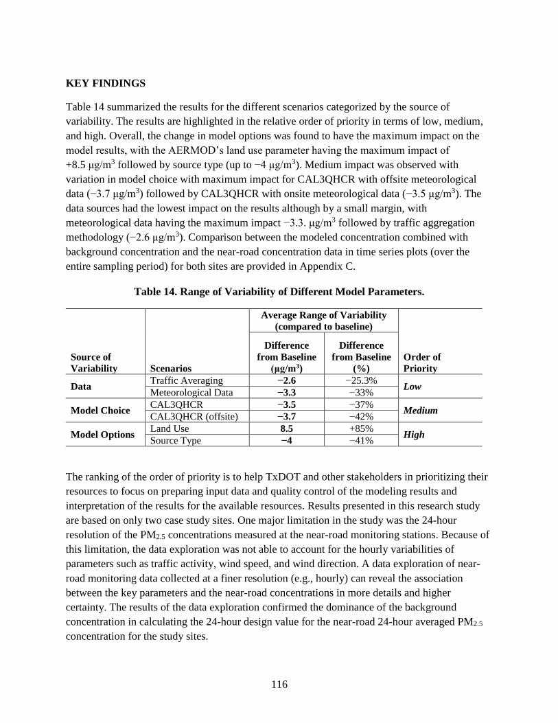
116
KEY FINDINGS
Table 14 summarized the results for the different scenarios categorized by the source of
variability. The results are highlighted in the relative order of priority in terms of low, medium,
and high. Overall, the change in model options was found to have the maximum impact on the
model results, with the AERMOD’s land use parameter having the maximum impact of
+8.5 μg/m3 followed by source type (up to −4 μg/m3). Medium impact was observed with
variation in model choice with maximum impact for CAL3QHCR with offsite meteorological
data (−3.7 μg/m3) followed by CAL3QHCR with onsite meteorological data (−3.5 μg/m3). The
data sources had the lowest impact on the results although by a small margin, with
meteorological data having the maximum impact −3.3. μg/m3 followed by traffic aggregation
methodology (−2.6 μg/m3). Comparison between the modeled concentration combined with
background concentration and the near-road concentration data in time series plots (over the
entire sampling period) for both sites are provided in Appendix C.
Table 14. Range of Variability of Different Model Parameters.
Source of
Variability Scenarios
Average Range of Variability
(compared to baseline)
Order of
Priority
Difference
from Baseline
(μg/m3)
Difference
from Baseline
(%)
Data Traffic Averaging −2.6 −25.3%
Low Meteorological Data −3.3 −33%
Model Choice CAL3QHCR −3.5 −37%
Medium CAL3QHCR (offsite) −3.7 −42%
Model Options Land Use 8.5 +85%
High Source Type −4 −41%
The ranking of the order of priority is to help TxDOT and other stakeholders in prioritizing their
resources to focus on preparing input data and quality control of the modeling results and
interpretation of the results for the available resources. Results presented in this research study
are based on only two case study sites. One major limitation in the study was the 24-hour
resolution of the PM2.5 concentrations measured at the near-road monitoring stations. Because of
this limitation, the data exploration was not able to account for the hourly variabilities of
parameters such as traffic activity, wind speed, and wind direction. A data exploration of near-
road monitoring data collected at a finer resolution (e.g., hourly) can reveal the association
between the key parameters and the near-road concentrations in more details and higher
certainty. The results of the data exploration confirmed the dominance of the background
concentration in calculating the 24-hour design value for the near-road 24-hour averaged PM2.5
concentration for the study sites.

117
Together, the data exploration research and modeling analyses highlight the fact that both the
near-road air quality and the PM hot-spot modeling process are complex, involving a myriad of
parameters and factors on both the distribution and quantification of the PM concentrations. The
results highlighted significant variation as a result of typical modeling options and data sources
used in conducting a PM hot-spot analysis. These factors are found to impact both at an
individual level and at a cumulative level. The availability of the near-road data presents an
opportunity to qualitatively evaluate the different variabilities involved in the hot-spot process
qualitatively. It is very important for the air quality modelers and stakeholders to be aware of
these variations and interpret the results in the proper context.


119
CHAPTER 8:
FINDINGS AND CONCLUSIONS
This research project explored the potential of using the near-road concentration data measured
at near-road monitors in evaluating the potential variabilities involved in the regulatory PM hot-
spot process. The project involved the following main elements:
• State-of-the-practice review.
• Data exploration research of the near-road monitoring observations to evaluate the
potential association between the near-road PM2.5 concentrations and the key factors.
• Sensitivity analysis to evaluate the variabilities of the modeling process involved in the
regulatory PM hot-spot analysis for key parameters.
The state-of-the-practice review highlights the emergence of real-world air quality data from
near-road monitoring stations in the recent years that can be used for various applications. Also,
it identifies a gap in the current research in evaluating the variabilities involved in the modeling
components of the PM hot-spot process used to evaluate near-road pollutant concentration levels.
Combining the two, this new source of real-world data can be explored to assess the variabilities
involved with the PM hot-spot process. Two sites (Houston and Fort Worth) were selected based
on different selection metrics for detailed data exploration (Track 1) and model sensitivity
analysis (Track 2).
The key findings from this research project are as follows.
TRACK 1—DATA EXPLORATION
Researchers performed a data exploration research on the near-road monitoring data to evaluate
the potential association between the near-field pollutant concentrations and key meteorological,
traffic, and background concentration data. The key findings from the data exploration effort are
summarized as follows:
• The descriptive statistics from the near-road monitoring stations indicate that at both sites
the concentrations of CO, PM2.5, and NO2 appear to be below the NAAQS limits based
on the data available. This simple comparison with NAAQS is only for research purposes
and is performed as an initial step of understanding the range of the data.
• Both wind direction and wind speed are found to have an influence on CO and NO2.
Higher concentration levels are found to occur during low wind speeds and downwind
conditions (i.e., when the monitor is downwind from the freeway). This observation
demonstrates that traffic during downwind conditions could be a major factor influencing
the distribution of CO and NO2 levels. PM2.5 concentrations were found to be more
widely distributed in both southwest and southeast directions, indicating there could be
other factors that influence the concentration distributions.

120
• A relatively weak correlation between freeway traffic parameters (AADT, FE-AADT,
volume, and traffic speed) and near-road concentrations of PM2.5 was observed. During
the downwind conditions, traffic parameters are found to have more impact on NO2 and
CO levels.
• The determination coefficient (R2) for near-road PM2.5 and background PM2.5 levels
varied between 0.83 and 0.91. Changes in concentrations of near-road PM2.5 are found to
correlate more with changes in concentrations of nearby ambient monitors representing
regional contribution than with any other parameters.
• On average, the near-road increment (i.e., the difference between the near-road
concentration and background concentration) was found to be 2.4 µg/m3 (or
12.8 percent). This increment could be attributed to the potential impact of traffic
measured at the near-road monitors.
TRACK 2—MODELING SENSITIVITY ANALYSIS
Researchers formulated 10 scenarios to evaluate the variability for different data sources, model
options, and model choices involved in the PM2.5 hot-spot process. Researchers evaluated the
scenarios in the form of probably density histograms and qualitatively compared the scenarios to
the near-road monitoring data to investigate the key components affecting the sensitivity of the
modeling process. The key findings from the modeling sensitivity analysis effort are summarized
as follows:
• The modeling exercise points to the fact that are many factors in the PM hot-spot process
that impact the estimated concentrations. These factors are found to affect the PM
concentration estimates both at the individual modeling element level and cumulative
across the entire modeling chain.
• The results highlight the importance of careful selection and processing of input
parameters for activity/traffic, emissions, and air dispersion components. As highlighted
by the sensitivity analysis, quality assurance at every step of the modeling process is
required to ensure valid concentration results.
• The relationship between modeling and decision-making can be enhanced by reporting
the outcomes of modeling in terms of distribution or ranges in addition to reporting the
outcome of single design value. The distribution information would provide a better
understanding of the variabilities in the modeling results and help interpret the results in
the proper context.
• Communicating the modeling results in probability density histograms would help
demonstrate that the modeling process produces a range of concentrations (i.e., a
spectrum of likely concentrations) in addition to the single design value representing a
specific risk to the human health as formulated by EPA.

121
In conclusion, the findings from this study provided a systematic assessment of the variabilities
in the hot-spot modeling results as caused by different assumptions and parameters and provided
an evaluation of the impact of traffic activities and other factors on the near-road PM2.5
concentrations. Overall, the findings indicate that the background concentration is the
dominating factor in estimating the near-road PM2.5 concentrations. Traffic volume and speed
were found to have a relatively weak association with the near-road concentrations. Wind
direction and speed were found to have a correlation with the concentrations; however, the lack
of hourly near-road concentrations data at the time of this study prevented researchers from a
detailed analysis of this potential correlation at an hourly resolution.
The results of the modeling variability analysis highlighted significant variations of the estimated
near-road concentrations as a result of typical modeling options and data sources used in
conducting a PM hot-spot analysis. The range of variability was highest for the land use selection
option (up to 8.5 μg/m3) and lowest for traffic averaging method (up to 2.6 μg/m3). Researchers
used several methods to estimate the background concentration, including the recommended
method in the PM hot-spot analysis guidance document. The background results from the two
study sites showed a low variability among the different methods (up to 1.1 μg/m3).
During this project, researchers identified several areas of future research that can build on the
project findings and advance better understanding of the PM hot-spot modeling results and
potential applications of near-road monitoring data in evaluating the net impact of traffic on the
near-road environment. Potential areas of future research are as follows:
• The use of real-world travel time and traffic data obtained from radar sensors, GPS,
cellphone, or similar sources to study detailed traffic behavior around the study sites.
These data sources can provide data that are representative of real-world behavior, for a
large sample of vehicles, in a cost-effective manner.
• Conducting further investigation of the near-road monitoring data to build a detailed
understanding of the true impact of traffic activities on near-road air quality and potential
improvements to the quantitative hot-spot analysis process. Researchers identified the
following opportunities for further research on near-road monitoring data:
− This study focused on the PM2.5 concentrations. An opportunity exists to expand the
data exploration to other pollutants that are being measured at the near-road
monitoring stations (e.g., NO2 and CO).
− The near-road PM2.5 monitoring data that were available at the time of this study had
a 24-hour resolution. The lack of hourly near-road concentrations data limited the
scope of the data research performed in this study. There are now two near-road
monitoring sites in Texas (Austin and San Antonio) that measure PM2.5
concentrations at an hourly resolution. A data exploration of these hourly
observations can provide better understanding of the impact of traffic activity and
other parameters on the near-road air quality.

122
− At the time of this study, only one complete year of near-road concentration data was
available. In addition to making a larger sample, the design values could be
established using data from three or more complete years. The design value could be
used for more detailed comparison with the modeling results.
• Accurate estimation of background concentrations is a critical component of estimating
the design value in the hot-spot analysis. Researchers developed a novel approach to
select the best methodology for a specific site. This approach is based on the evaluation
of analytical seven methods using data from multiple background ambient monitoring
stations and applying a resampling technique. This approach was applied to the two case
studies performed in this project. The results showed a relatively low variability among
the different methods, which may be caused by a relatively flat terrain and urban land
use. It is recommended to evaluate the performance of the proposed approach for a more
diverse set of areas and investigate potential trends and opportunities for streamlining this
important step of the hot-spot analysis.
• The sensitivity analysis of the PM2.5 hot-spot analysis modeling process that was
conducted in this study included two case study sites that are in warm climate, urban land
use, and in a relatively flat terrain. A modeling sensitivity analysis to include monitoring
sites across a diverse set of geographic scales, configurations, climates, and land uses
would provide a better understanding of the overall trends in near-road air quality. This
knowledge would be very important in revising and streamlining the hot-spot analysis
process.
• The availability of the near-road data has created an opportunity to explore whether the
data can be used for screening purposes and streaming the hot-spot analysis for a
particular pollutant.

123
REFERENCES
[1] Benson and P. E, “Caline4 - a Dispersion Model for Predicting Air Pollutant
Concentrations Near Roadways. Final Report,” Calif. Dep. Transp., vol. FHWA/CA/TL,
p. 277, 1984.
[2] US EPA, “Addendum to the User’s Guide to CAL3QHC Version 2.0 (CAL3QHCR
User’s Guide),” 1995.
[3] US EPA, “Appendix W to Part 51—Guideline on Air Quality Models,” 2015. [Online].
Available: https://www3.epa.gov/ttn/scram/appendix_w-2016.htm. [Accessed: 24-Jun-
2019].
[4] U.S. Environmental Protection Agency, “Guideline on Air Quality Models,” Fed. Regist.,
vol. 82, no. 10, pp. 5182–5235, 2017.
[5] A. A. Karner, D. S. Eisinger, and D. A. Niemeier, “Near-roadway air quality:
Synthesizing the findings from real-world data,” Environ. Sci. Technol., vol. 44, no. 14,
pp. 5334–5344, 2010.
[6] A. Venkatram, M. Snyder, V. Isakov, and S. Kimbrough, “Impact of wind direction on
near-road pollutant concentrations,” Atmos. Environ., vol. 80, pp. 248–258, Dec. 2013.
[7] Code of Federal Register, “Title 40CFR Part 58.10,” 2017.
[8] N. S. Holmes and L. Morawska, “A review of dispersion modelling and its application to
the dispersion of particles: An overview of different dispersion models available,” Atmos.
Environ., vol. 40, no. 30, pp. 5902–5928, Sep. 2006.
[9] US EPA, “Transportation Conformity Guidance for Quantitative Hot - spot Analyses in
PM 2.5 and PM 10 Nonattainment and Maintenance Areas,” 2010.
[10] US EPA, “User’s Guide to CAL3QHC Version 2.0: A Modeling Methodology for
Predicting Pollutant Concentrations Near Roadway Intersections (Revised).” Office of Air
Quality Planning and Standards, Research Triangle Park, NC, p. EPA-454/R-92-006R,
1995.
[11] A. J. Cimorelli et al., “AERMOD: A Dispersion Model for Industrial Source Applications.
Part I: General Model Formulation and Boundary Layer Characterization,” J. Appl.
Meteorol., vol. 44, no. 5, pp. 682–693, May 2005.
[12] US EPA, “Addendum User’s Guide for the Aermod Meteorological Preprocessor,” 2011.
[13] US EPA, “AERMOD : Description of model formulation,” 2004.
[14] D. B. Turner, Workbook of atmospheric dispersion estimates : an introduction to
dispersion modeling. Lewis Publishers, 1994.

124
[15] R. R. Peter, K. O. Pinkerman, E. C. Shirley, and California. Transportation Laboratory.,
Variables affecting air quality instrument operation : interim report. 1977.
[16] S. H. Cadle, D. P. Chock, P. R. Monson, and J. M. Heuss, “General Motors Sulfate
Dispersion Experiment: Experimental Procedures and Results,” J. Air Pollut. Control
Assoc., vol. 27, no. 1, pp. 33–38, Jan. 1977.
[17] M. Claggett, J. Shrock, and K. E. Noll, “Carbon monoxide near an urban intersection,”
Atmos. Environ., vol. 15, no. 9, pp. 1633–1642, Jan. 1981.
[18] C. E. Rodes and D. M. Holland, “Variations of NO, NO2 and O3 concentrations
downwind of a Los Angeles freeway,” Atmos. Environ., vol. 15, no. 3, pp. 243–250, Jan.
1981.
[19] US EPA, “AERMOD: Latest Features and Evaluation Results,” 2003.
[20] M. Barad, Project Prairie Grass, a field program in diffusion. Bedford Mass.: United
States Air Force Air Research and Development Command Air Force Cambridge
Research Center Geophysical Research Directorate Atmospheric Analysis Laboratory,
1958.
[21] M.-K. Liu and G. E. Moore, “Diagnostic validation of plume models at a plains site,” Rep.
EPRI/Elektric power Res. inst., 1984.
[22] Anon, “URBAN POWER PLANT PLUME STUDIES.,” Jan. 1988.
[23] N. E. Bowne, R. J. Londergan, D. R. Murray, and H. S. Borenstein, “Overview, results,
and conclusions for the EPRI plume model validation and development project: Plains
Site. EPRI EA--3074,” Electr. Power Res. Institute, Palo Alto, CA, 1983.
[24] D. B. Turner, L. W. Bender, and J. O. Paumier, “EVALUATION OF THE TUPOS AIR
QUALITY DISPERSION MODEL USING DATA FROM THE EPRI KINCAID FIELD
STUDY,” Atmos. Environ., vol. 25, no. 10, pp. 2187–2201, 1991.
[25] S. R. Hanna and J. C. Chang, “Hybrid plume dispersion model (HPDM) improvements
and testing at three field sites,” Atmos. Environ. Part A. Gen. Top., vol. 27, no. 9, pp.
1491–1508, Jun. 1993.
[26] TRC, “Evaluation of Rural Air Quality Simulation Models,” Research Triangle Park, NC,
1982.
[27] TRC, “Air Quality Model Performance Evaluation and Comparison Study for Martins
Creek Steam Electric Station,” Windsor, CT, 1994.
[28] H. Zhou and D. Sperling, “Traffic emission pollution sampling and analysis on urban
streets with high-rising buildings,” Transp. Res. Part D Transp. Environ., vol. 6, no. 4, pp.
269–281, Jul. 2001.

125
[29] S. Gokhale and N. Raokhande, “Performance evaluation of air quality models for
predicting PM10 and PM2.5 concentrations at urban traffic intersection during winter
period,” Sci. Total Environ., vol. 394, no. 1, pp. 9–24, May 2008.
[30] S. A. Abdul-Wahab, “An Application and Evaluation of the CAL3QHC Model for
Predicting Carbon Monoxide Concentrations from Motor Vehicles Near a Roadway
Intersection in Muscat, Oman,” Environ. Manage., vol. 34, no. 3, pp. 372–382, Sep. 2004.
[31] V. Jacomino, F. Tavares, A. Barreto, and E. Dutra, “Study of the dispersion process of
vehicular emissions at a specific site in Belo Horizonte using numerical simulation,” in
WIT Transactions on Biomedicine and Health, 2009, vol. 14, pp. 23–34.
[32] B. Zou, Y. Zeng, H. Liu, H. Zhang, Y. Qiu, and B. F. Zhan, “Sensitivity analysis of
AERMOD in modeling local air quality under different model options,” 2010 4th Int.
Conf. Bioinforma. Biomed. Eng. iCBBE 2010, pp. 1–4, 2010.
[33] G. E. Long and G. E. Long, “An analysis of AERMOD sensitivity to input parameters in
the San Francisco Bay Area.” AMS, 24-Aug-2004.
[34] R. Steib, “Regulatory Modelling Activity in Hungary,” in Advances in Air Pollution
Modeling for Environmental Security, Berlin/Heidelberg: Springer-Verlag, pp. 337–347.
[35] W. B. Faulkner, B. W. Shaw, and T. Grosch, “Sensitivity of Two Dispersion Models
(AERMOD and ISCST3) to Input Parameters for a Rural Ground-Level Area Source,” J.
Air Waste Manage. Assoc., vol. 58, no. 10, pp. 1288–1296, Oct. 2008.
[36] E. Carper and E. Ottersburg, “Sensitivity Analysis Study Considering the Selection of
Appropriate L…,” 2004.
[37] A. J. Schroeder and G. J. Schewe, “Sensitivity of AERMOD to Meteorological Data Sets
Based on Varying Surface Roughness,” in Air and Waste Management Annual Conference
and Exhibition, 2009, pp. 1–15.
[38] M. Claggett, “Comparing Predictions from the CAL3QHCR and AERMOD Models for
Highway Applications,” Transp. Res. Rec. J. Transp. Res. Board, vol. 2428, no. 2, pp. 18–
26, 2014.
[39] K. Westerlund and C. Cooper, “Modeling Concentrations of Air Toxics near Intersections
and Freeways in Florida,” J. Environ. Eng., vol. 140, no. 1, p. pp 92-99, Jan. 2014.
[40] S. Vallamsundar and J. Lin, “Sensitivity Test Analysis of MOVES and AERMOD
models,” 92nd Transportation Research Board Annual Meeting, vol. paper #13-. p. 19,
2013.
[41] Z. Radonjic, D. B. Chambers, and J. Kikaldy, “Modelling Line Sources (Roads) Using
CAL3QHCR, ISC3, AERMOD and CALPUFF,” in Air and Waste Management Annual
Conference and Exhibition, 2003.

126
[42] P. By, J. Lin, and S. Vallamsundar, “TRANSPORTATION CONFORMITY
PARTICULATE MATTER HOT-SPOT AIR QUALITY MODELING Transportation
Conformity Particulate Matter Hot-Spot Air Quality Modeling Illinois Center for
Transportation,” 2013.
[43] D. Heist et al., “Estimating near-road pollutant dispersion: A model inter-comparison,”
Transp. Res. Part D Transp. Environ., vol. 25, pp. 93–105, Dec. 2013.
[44] H. Chen, S. Bai, D. Eisinger, D. Niemeier, and M. Claggett, “Predicting Near-Road PM 2.5
Concentrations,” Transp. Res. Rec. J. Transp. Res. Board, vol. 2123, no. 1, pp. 26–37,
Jan. 2009.
[45] M. Claggett, “Improvements to the CAL3QHCR Model,” 2014.
[46] A. Pasch, S. Bai, D. Eisinger, K. Craig, J. Andrews, and J. P. Elder, “PM Hot-Spot
Analysis Using AERMOD and EMFAC2011: Technical Issues and Lessons Learned,” in
Transportation Research Board Annual Meeting, 2012.
[47] L. Yu et al., PEMS-based Approach to Developing and Evaluating Driving Cycles for Air
Quality Assessment. Center for Transportation Training and Research, Texas Southern
University, 2010.
[48] U. EPA, “Overview of the Clean Air Act and Air Pollution.”
[49] N. W. Service, “NWS GIS Portal.” [Online]. Available: https://www.weather.gov/gis/.
[Accessed: 24-Jun-2019].
[50] USGS, “Land Use Database,” 2017. [Online]. Available:
https://archive.usgs.gov/archive/sites/landcover.usgs.gov/index.html. [Accessed: 24-Jun-
2019].
[51] J. L. DeWinter, S. G. Brown, A. F. Seagram, K. Landsberg, and D. S. Eisinger, “A
national-scale review of air pollutant concentrations measured in the U.S. near-road
monitoring network during 2014 and 2015,” Atmos. Environ., vol. 183, no. April, pp. 94–
105, 2018.
[52] S. Vallamsundar and J. Lin, “Sensitivity Test Analysis of MOVES and AERMOD
models,” in 92st Annual Meeting of the Transportation Research Board, 2013.
[53] M. P. Keuken et al., “Source contributions to PM2.5 and PM10 at an urban background
and a street location,” Atmos. Environ., vol. 71, no. x, pp. 26–35, 2013.
[54] FHWA, “Detailed Monitoring Protocol for U.S. 95 Settlement Agreement. National Near-
Road Study 2017,” 2017.
[55] H. A. Olvera, M. Lopez, V. Guerrero, H. Garcia, and W.-W. Li, “Ultrafine particle levels
at an international port of entry between the US and Mexico: Exposure implications for
users, workers, and neighbors,” J. Expo. Sci. Environ. Epidemiol., vol. 23, no. 3, pp. 289–

127
298, 2013.
[56] I. G. Mckendry, “Background Concentrations of PM 2.5 and Ozone in British Columbia,
Canada EXECUTIVE SUMMARY,” 2006.
[57] J. L. DeWinter, S. G. Brown, A. F. Seagram, K. Landsberg, and D. S. Eisinger, “A
national-scale review of air pollutant concentrations measured in the U.S. near-road
monitoring network during 2014 and 2015,” Atmos. Environ., vol. 183, pp. 94–105, Jun.
2018.
[58] S. Arunachalam et al., “A Method for Estimating Urban Background Concentrations in
Support of Hybrid Air Pollution Modeling for Environmental Health Studies,” Int. J.
Environ. Res. Public Health, vol. 11, no. 10, pp. 10518–10536, Oct. 2014.
[59] G. Hoek et al., “A review of land-use regression models to assess spatial variation of
outdoor air pollution,” Atmos. Environ., vol. 42, no. 33, pp. 7561–7578, Oct. 2008.
[60] J. A. Araujo, “Particulate air pollution, systemic oxidative stress, inflammation, and
atherosclerosis.,” Air Qual. Atmos. Health, vol. 4, no. 1, pp. 79–93, Nov. 2010.
[61] B. Hoffmann et al., “Residential Exposure to Traffic Is Associated With Coronary
Atherosclerosis,” Circulation, vol. 116, no. 5, pp. 489–496, Jul. 2007.
[62] A. Iannuzzi et al., “Air pollution and carotid arterial stiffness in children,” Cardiol.
Young, vol. 20, no. 2, pp. 186–190, Apr. 2010.
[63] R. X. Armijos, M. M. Weigel, O. B. Myers, W.-W. Li, M. Racines, and M. Berwick,
“Residential Exposure to Urban Traffic Is Associated with Increased Carotid Intima-
Media Thickness in Children,” J. Environ. Public Health, vol. 2015, pp. 1–11, 2015.
[64] F. D. Gilliland et al., “The effects of ambient air pollution on school absenteeism due to
respiratory illnesses.,” Epidemiology, vol. 12, no. 1, pp. 43–54, Jan. 2001.
[65] L. Lei Chen, Brian L. Jennison, Wei Ya, B. L. Jennison, W. Yang, and S. T. Omaye,
“Elementary School Absenteeism and Air Pollution,” Inhal. Toxicol., vol. 12, no. 11, pp.
997–1016, Jan. 2000.
[66] J. K. Wendt, E. Symanski, T. H. Stock, W. Chan, and X. L. Du, “Association of short-
term increases in ambient air pollution and timing of initial asthma diagnosis among
medicaid-enrolled children in a metropolitan area,” Environ. Res., vol. 131, pp. 50–58,
May 2014.
[67] Office of Research & Development, “EPA’S EMERGING NEAR-ROAD AMBIENT
MONITORING NETWORK: A PROGRESS REPORT,” 2013.
[68] Government Publishing Office, “Federal Register Title 40CFR Part 58, Appendix D.,”
2017.

128
[69] T. A. Cahill et al., “Artificial ultra-fine aerosol tracers for highway transect studies,”
Atmos. Environ., vol. 136, pp. 31–42, Jul. 2016.
[70] TCEQ, “Air Dispersion Modeling Team Initiative to Update Meteorological Data,” 2013.
[71] Government Publishing Office, “Federal Register Vol. 81, No 251.,” 2016.
[72] Code of Federal Regulations, “Appendix E to Part 58—Probe and Monitoring Path Siting
Criteria for Ambient Air Quality Monitoring.” [Online]. Available:
https://www.ecfr.gov/cgi-
bin/retrieveECFR?gp=&r=PART&n=40y6.0.1.1.6#ap40.6.58.0000_0nbspnbspnbsp.e.
[Accessed: 25-Jun-2019].
[73] Texas Commission on Environmental Quality, “2016 Annual Monitoring Network Plan.”
[74] Code of Federal Register, “Title 40CFR Part 58, Appendix D, Section 3.0.,” 2017.
[75] Code of Federal Register, “Title 40CFR Part 58, Appendix D, Section 5.0.,” 2017.
[76] Code of Federal Register, “Title 40CFR Part 58, Appendix D, Section 4.2.,” 2017.
[77] Code of Federal Register, “Title 40CFR Part 58, Appendix D, Section 4.7.,” 2017.
[78] H. Ginzburg et al., “Monitoring study of the near-road PM 2.5 concentrations in
Maryland,” J. Air Waste Manage. Assoc., vol. 65, no. 9, pp. 1062–1071, Sep. 2015.
[79] I. Sonoma Technology, “National Near-Road Data Assessment: Draft Report No. 2 With
2015 Data,” 2016.
[80] TCEQ, “Meteorological Data Sets for AERMOD.,” 2016.
[81] Midwestern Software Solutions, “MS2 Transportation Traffic Analytics.” [Online].
Available: https://www.ms2soft.com/. [Accessed: 24-Jun-2019].
[82] TxDOT, “Traffic Count Database System (TCDS).” [Online]. Available:
https://txdot.ms2soft.com/tcds/tsearch.asp?loc=Txdot&mod=TCDS. [Accessed: 24-Jun-
2019].
[83] US EPA, “Near-road NO2 Monitoring Technical Assistance Document EPA-454/B-12-
002,” Research Triangle Park, NC, 2012.
[84] Texas A&M Transportation Institute, “MOVES2014a-Based Travel Demand Model Link
Emissions Estimation Method,” 2016.
[85] US EPA, “AP-42: Section 13.2.1 Paved Roads,” 2016.
[86] US EPA, “Heat Island Effect,” 2016.
[87] USEPA, “Interim Joint Technical Assessment Report: Light-Duty Vehicle Greenhouse

129
Gas Emission Standards and Corporate Average Fuel Economy Standards for Model
Years 2017-2025,” 2010.
[88] US EPA, “Air Quality Dispersion Modeling - Preferred and Recommended Models
AERMOD.”
[89] B. Efron and R. Tibshirani, An introduction to the bootstrap. Chapman & Hall, 1994.
[90] G. J. Schewe, “Using AERMOD in PM2.5 and PM10 Conformity Hot-Spot Analysis,” in
Transportation Planning, Land Use, and Air Quality Conference, 2011.
[91] US EPA, “ATTACHMENT A Critical Design Value Estimation and Its Applications,”
2011.
[92] US EPA, “National Ambient Air Quality Standards for Particulate Matter.”
[93] M. J. Barnes et al., “Spatially-varying surface roughness and ground-level air quality in an
operational dispersion model,” Environ. Pollut., vol. 185, pp. 44–51, 2014.
[94] N. W. S. US Department of Commerce, NOAA, “NWS GIS Portal.” [Online]. Available:
https://www.weather.gov/gis/. [Accessed: 20-Nov-2018].
[95] USGS, “The USGS Land Cover Institute (LCI).” [Online]. Available:
https://landcover.usgs.gov/. [Accessed: 20-Nov-2018].
[96] US EPA, “User Guide for the Aermod Meteorological Preprocessor User Guide for the
Aermod Meteorological Preprocessor,” Research Triangle Park, NC, 2016.
[97] M. O’Donnel, “Course # 296 Health Risk Assessments and Dispersion Modeling.” 2014.
[98] US EPA, “AERSURFACE User’s Guide,” 2013.
[99] US EPA, “PCRAMMET USER’S GUIDE,” 1999.
[100] US EPA, “User Instructions: Computing Twice-Daily Mixing Heights from Upper Air
Soundings and Hourly Temperatures,” 1998.
[101] US EPA, “Memo: Procedures for Substituting Values for Missing NWS Meteorological
Data for Use in Regulatory Air Quality Models.” 1992.


131
APPENDIX A: METEOROLOGICAL DATA
A detailed overview of the meteorological data processing for AERMOD, and CAL3QHCR is
provided in sections A1, and A2, respectively. Section A3 overviews the methodology that was
used to achieve consistency between the meteorological data files between the two models.
METEOROLOGICAL DATA PROCESSING FOR AERMOD
Meteorological conditions strongly impact the pollutant dispersion in the atmosphere. Three
types of data are required for processing the meteorological data, namely, surface data that
measure characteristics of lower layers of the atmosphere, upper air data that measure
characteristics that change with height in the atmosphere (such as temperature), and land use data
that represent surface characteristics. For this study, the raw meteorological and land use data
were obtained from the following sources:
• Automated Surface Observing Stations (ASOS).
• National Weather Station databases (NWS).
• U.S. Geological survey land use database (USGS).
The ASOS and NWS databases are owned and maintained by NCDC and National Oceanic and
Atmospheric Administration (NOAA) under the U.S. Department of Commerce [94]. USGS land
use database is a national archive for remotely sensed images of Earth’s land surface maintained
by the U.S. Department of the Interior [95]. USGS land use database is a national archive for
remotely sensed images of Earth’s land surface maintained by the U.S. Department of the
Interior. Figure A1 shows the process of meteorological data processing for AERMOD. The raw
data are processed using meteorological preprocessors namely, AERMINUTE, AERMET, and
AERSURFACE to produce data in a format compatible for AERMOD. High resolution wind
data are processed by AERMINUTE preprocessor in the first step. One of the main concerns in
using NWS surface data directly for AERMOD is the presence of high incidence of calm and
missing wind data. AERMOD cannot accurately simulate dispersion with calm/missing winds.
To reduce this, NCDC started archiving raw one-minute data logged by automated stations.
AERMINUTE is used to process the one-minute data to produce hourly wind speed and direction
averages to improve the quality of surface data obtained from the NWS. The second step consists
of obtaining the land cover surface characteristics from the AERSURFACE preprocessor.
AERSURFACE processes the land cover data (specific to the case study location) from the
USGS database and produces surface characteristics.

132
Figure A1. Meteorological and Land Use Processing for AERMOD.
These surface characteristics relate to the following parameters:
• Albedo: fraction of total incident solar radiation that is reflected back to space without
absorption.
• Bowen ratio: amount of surface moisture conditions.
• Surface roughness (height of obstacles to the wind flow).
In the third step, AERMET incorporates surface and upper data from the NWS database and
combines them with the hourly wind speed and direction averages produced by AERMINUTE
and land cover surface data (albedo, surface roughness, and Bowen’s ratio) from AERSURFACE
to produce output files for AERMOD. The two files produced by AERMET consist of a
boundary layer parameter (.SFC) file that includes turbulence parameters, mixing height, and
friction velocity. The second file (.PFL) contains the vertical profile of winds, temperature, and
standard deviation of the fluctuating components of the wind. These two files are directly
incorporated into AERMOD. According to EPA [12], AERMET shall be used to preprocess all
meteorological data, be it observed or prognostic, for use with AERMOD in regulatory
applications, and the AERMINUTE processor, in most cases, should be used to process 1-minute
ASOS wind data for input to AERMET when processing NWS ASOS sites in AERMET.
Meteorological Files Required by AERMET
Details of the input files required by AERMET meteorological preprocessor is provided in this
section.

133
Surface Input
The surface input file is acquired from NCDC of NOAA. The hourly surface data for all
available years are placed in a file transfer protocol server at the link
ftp://ftp.ncdc.noaa.gov/pub/data/noaa/. The users can identify the desired stations and years of
data by looking up the table in the file, isd_history.txt, located in the ftp site.
Onsite Input
The onsite input file has to be created based on what parameters are desired in accordance to
input requirements as specified by EPA [96]. Each column of the created data set should
represent one parameter. For this project, the parameters to be used are day, month, year, hour,
precipitation amount, temperature, dew point temperature, wind speed, wind direction, standard
deviation of horizontal wind, and relative humidity. The data for these parameters can be
retrieved, as a CSV file, from NOAA’s Local Climatological Data at the link
https://www.ncdc.noaa.gov/cdo-web/datatools/lcd. The Texas Commission on Environmental
Quality (TCEQ) also provides a number of selected years of site-specific onsite data for many
Texas air monitoring stations, and the parameters can also be found at their TAMIS website.
Upper Air Input
Upper air data are recorded at unevenly, sparsely distributed locations throughout the United
States. Selection of the closest upper air data for use in air dispersion modeling requires special
attention as only certain stations record data at a certain time so the closest upper air station to
the point of interest can be far away from the modeling domain. The data can be retrieved from
NOAA’s Radiosonde Database at https://ruc.noaa.gov/raobs/.
AERMINUTE Input
A potential concern related to the use of ISD meteorological data for air dispersion modeling is
the often high incidence of calms and variable wind conditions. In the reporting of surface
weather data, a calm wind is defined as a wind speed less than 3 knots and is assigned a value of
0 knots. In addition, the wind direction may be reported as missing if the wind direction varies
more than 60 degrees during the 2-minute averaging period for the observation [97]. To reduce
the number of calms and missing winds in the surface data, the 1-minute ASOS wind data are
used to calculate hourly average wind speed and directions, which are used to backfill the
missing data and calms in the ISD data. This ASOS minute data can be found in the NCDC
database, the same link as the previously discussed surface data. The ASOS data contain both
TD 6405 and TD 6406 formatted files. For the purpose of creating a meteorological file, the data
start with 6405 followed by the desired year were used. As the ASOS minute files are unusually
large, they need to be downloaded separately based on the months required.

134
AERSURFACE Input
The AERSURFACE processor is developed to compute surface characteristic values such as
albedo, Bowen ratio, and surface roughness length, in a modeling domain for use in AERMET
[98]. Similar to AERMINUTE, data from AERSURFACE can be created or simplified by
dividing the area of study into different sectors and giving each sector an albedo, Bowen ratio,
and surface roughness. For this project, the AERSURFACE program was run using National
Land Cover Data from 1992 (NLCD 92) from the United States Geological Survey at the
following link: https://www.mrlc.gov/viewerjs/.
Meteorological Files Generated by AERMET
Five consecutive years (2012–2016) of off-site surface meteorological data were generated for
use in the dispersion modeling for both Houston and Fort Worth near-road case study sites. Two
years (2015–2016) of site-specific meteorological parameters were generated from AERMET by
using the on-site data from the near-road monitoring stations (TCEQ’s CAMS C1052 and
C1053) in conjunction with respective upper air, ISD, and ASOS data. Each file is named with
index codes in the following fashion:
File Name= Site_Surface_Upper_Year_SR.File
Site = Onsite or offsite
Surface = Station ID for surface data
Upper = Station ID for upper air data
Year = year of data in 2 digits
SR = Surface Roughness (High: 1 m; Medium: 0.5 m; Low: 0.05 m; S: Site-specific from
AERSURFACE)
File = File extension, PFL for profile data and SFC for surface data
For example, File ONSITE_IAH_LCH_15H.SFC is the site-specific (ONSITE) hourly surface
data (SFC) for the year of 2015 using upper air data from Lake Charles (LCH), surface data from
Houston International Airport (IAH), and surface roughness of 1 m (H) for AERMOD modeling.
METEOROLOGICAL DATA PROCESSING FOR CAL3QHCR
Unlike AERMOD, CAL3QHCR can only process up to a year of hourly meteorological data. A
meteorological file for CAL3QHCR must include wind vector (degrees), wind speed
(meters/sec), ambient temperature (K), stability class, and mixing heights. These files can also be
created using available EPA auxiliary meteorological processors and meteorological data. Data
from the NWS or NCDC formatted data can be processed through EPA’s meteorological
processors and accessory programs such as, the Meteorological Processor for Regulatory Models
(MPRM), PCRAMMET, or RAMMET programs, as recommended by EPA [99]. However,
currently NCDC has ceased to process NWS or NCDC formatted data for use in any of the
meteorological processors.

135
Among the EPA-recommended meteorological processors, PCRAMMET is selected for this
study because it has been widely used by EPA in preparing NWS data for use in the Agency’s
short-term air quality dispersion models such as CAL3QHCR, ISCST3, CRSTER, RAM,
MPTER, BLP, SHORTZ, and COMPLEX1 [96]. The minimum input data requirements to
PCRAMMET are the twice-daily mixing heights, hourly surface observations of wind speed and
wind direction, dry bulb temperature, opaque cloud cover, ceiling height, and station pressure, if
calculating dry deposition. These parameters can be obtained from the NCDC database with the
exception of the twice-daily mixing heights. Since the NCDC no longer provides the mixing
height data, it needs to be independently processed by using the EPA’s Mixing Height Program
(MIXHTS) program in conjunction with surface data and radiosonde upper air files [100].
Details of the input files required by PCRAMMET meteorological preprocessor is provided in
this section.
HUSWO Surface Meteorological Data
Both PCRAMMET and MIXHTS can read surface meteorological data in either HUSWO,
SCRAM, or CD-144 formats. Because the NCDC does not provide meteorological data in these
readable formats, data must be arranged in one of these formats using a text editor or other
methods. The HUSWO format was selected for this study to process on-site and off-site surface
meteorological data.
A combination of LCD data and ISD was used for creating the surface meteorological data files
for (a) its greater degree of completeness and inclusion of ceiling height and sky cover, required
inputs for MIXHTS and (b) maintaining data consistency between AERMET and PCRAMMET
outputs. Two years (2015–2016) of site-specific meteorological parameters (such as dry bulb
temperature, wind direction, and wind speed) for the Houston site were obtained from the TCEQ
CAM stations C1052 to develop site-specific meteorological files, and from C1053 for the Fort
Worth site.
Table A1 shows the HUWSO format parameters in the meteorological data file, units, and the
source and station code used to download meteorological data. Some parameters are not used in
CAL3QHCR or MIXHTS but must be included in the HUSWO format chosen; these parameters
are preserved in the file but filled with missing data identifiers. PCRAMMET assumes the
HUSWO data were retrieved in English units. Therefore, wind speeds in HUSWO are converted
from miles per hour to meters per second (m/s). Wind speeds below 1.0 m/s (calms included) are
set to 1.0 m/s before computations are made in PCRAMMET [99]. Missing wind direction and
wind speed values from the CAMS stations are replaced by the averages of the adjacent values,
the previous and next hour of data. This missing data treatment was performed for time periods
of less than 4 hours. Data missed for more than 4 hours are left untreated and flagged with
missing data. This method is recommended by the EPA for data sets that are less than 90 percent
complete [101].

136
Table A1. HUSWO Meteorological Data File.
Parameter Units Data Source Data Source Station
1 Station ID Station Number (WBAN) NCDC IAH, FTW
2 Time Year-Month-Day-Hour NCDC IAH, FTW
3 Global Radiation Nearest Tenth Watt Per Meter
Squared
- -
4 Direct Radiation Nearest Tenth Watt Per Meter
Squared
- -
5 Total Sky Cover Amount of Sky Dome (In Tenths)
Covered by Clouds. 99 = Missing
NCDC IAH, FTW
6 Opaque Sky Cover Amount of Sky Dome (In Tenths)
Covered by Clouds. 99 = Missing
NCDC IAH, FTW
7 Dry Bulb Temperature Degrees Fahrenheit TAMIS C1052, C1053
8 Dew Point Temp Degrees Fahrenheit NCDC IAH, FTW
9 Relative Humidity Percent NCDC IAH, FTW
10 Station Pressure Hundredths Of Inches NCDC IAH, FTW
11 Wind Direction Degrees TAMIS C1052, C1053
12 Wind Speed Miles Per Hour (Mph) TAMIS C1052, 1053
13 Visibility Miles NCDC IAH, FTW
14 Ceiling Height Feet IEM IAH, FTW
15 Present Weather Code NCDC IAH, FTW
16 ASOS Cloud Layer 1 Sky Condition Code 00-09 - -
17 ASOS Cloud Layer 2 Sky Condition Code 00-09 - -
18 ASOS Cloud Layer 3 Sky Condition Code 00-09 - -
19 Hourly Precipitation Hundredths of Inches NCDC IAH,FTW
20 Snow Depth Inches NCDC IAH, FTW
MIXHTS Mixing Height Data
MIXHTS requires two input files, the HUSWO surface file and a separate radiosonde upper air
data file, which can be obtained from the National Oceanic and Atmospheric Administration
(NOAA) database. The output of MIXHTS provides the mixing height data file needed for use in
PCRAMMET. Missing mixing height values were found with the previously stated method of
averaging the adjacent values from the previous and next entry of data.
Meteorological Files Generated by PCRAMMET
Meteorological files generated by PCRAMMET for CAL3QHCR modeling are named the same
way as discussed in Section A.2 with additional identifier in the extension:
File Name= Site_Surface_Upper_Year_SR.File
Site = Onsite or offsite
Surface = Station ID for surface data
Upper = Station ID for upper air data
Year = year of data in 2 digits

137
SR = Surface Roughness (N: not requires)
File = File extension, ISC for surface data.
For example, File ONSITE_IAH_LCH_15_N.ISC is the site-specific (ONSITE) hourly surface
data (ISC) for the year of 2015 using upper air data from Lake Charles (LCH), surface data from
Houston International Airport (IAH), and no specified surface roughness (N) for CAL3QHR
modeling.
CONSISTENCY BETWEEN AERMET AND PCRAMMET OUTPUTS
In order to evaluate the sensitivities of non-meteorology related parameters (such as source
characterization and time-varying emission) on the concentrations estimated by AERMOD and
CAL3QHR, it is important to ensure consistent meteorological data files are used for both
models. During the quality control process, researchers found that the hourly wind direction and
wind speed generated by AERMET and PCRAMMET did not agree with each other completely.
The ASOS 1-minute data are used to supplement the ISD surface hourly meteorological data in
AERMINUTE because ISD hourly surface meteorological data often include high incidence of
calms and variable wind conditions [97]. Although using the same ISD and ASOS data for the
same site, the algorithms used by NCDC (for processing the LCD and ISD combination file) and
by EPA (for processing the SFC file) to process the data appear to be different and may be the
reason for the discrepancies in wind direction and wind speed. In addition, there are inherent
differences in the reporting of wind speed among ISD, LCD, and TCEQ TAMIS. In reporting the
wind speed, LCD reports only integer mile/hr. winds whereas ISD and TCEQ TAMIS report to
one tenth of 1 m/sec.
In the treatment of calm condition, PCRAMMET assigns zero values for all wind speeds of less
than or equal to 1 m/sec whereas AERMET not only assigns zero values but also defaults the
wind direction to 0 degree for all wind speeds of less than or equal to 1 m/sec. On the contrary,
the TCEQ TRAMIS database (for site-specific data) reports wind speed to 0.1 m/sec with no
treatment of the wind direction. Both models treat the calm wind or missing meteorological data
conditions similarly. Both models set the concentration values to zero for that hour and calculate
the average by summing each valid (non-calm) 1-hour average concentration and dividing by the
total number of non-calm hours or 75 percent of the total number of hours in the period,
whichever is greater [2].
Consistency between the meteorological data files is achieved by replacing the wind speed and
wind direction in the ISC data files (used in CAL3QHCR) with the corresponding values in SFC
files (used in AERMOD) at the input stage of the CAL3QHCR file processing (i.e., before input
into MIXHTS and PCRAMMET). Figure A2 shows the general procedure followed in this study
in processing meteorological data from the input stage until the final stage data needed to ensure
consistency between the dispersion models.

138
SFC: AERMET output file WD: Wind Direction
PFL: AERMET output file LCD: Local Climatological Data
ISD: Integrated Surface Data system MIXHTS: EPA’s Mixing Height Program
WS: Wind Speed ISC: CAL3QHCR output file
Figure A2. Flowcharts for Consistency in Wind Direction and Wind Speed between
AERMET and PCRAMMET Outputs.

139
APPENDIX B: BACKGROUND CONCENTRATION
A detailed discussion of the analysis and results are provided in this appendix.
RESULTS AND DISCUSSION
The TCEQ PM2.5 monitoring network is designed to meet the SLAMS network and NCore
requirements [70]. This monitoring network provides data for near-road and regional background
applications. All background stations selected in this study were designed to support compliance
with NAAQS and research in air pollution studies (Title 40 CFR Part 58, Appendix D). They are
located at a distance clear of highway emissions (highway is considered as a roadway with more
than 50,000) and are representative of the area’s background concentration levels.
The 2-year quarterly time-series plots of the 24-hour average PM2.5 concentrations measured in
the Houston and Fort Worth areas are shown in Figure B1. Some high PM2.5 episodes recurring
around the same time of the year. For instance, high PM2.5 days occurred around middle of
March, May, June, and early July 7 each year for the Houston area, and around mid-June, and
early July and October 8 for the Fort Worth area. Furthermore, the time series data for the
background concentrations were noted to be strongly correlated with a well-defined trend for
both the case study sites. This is an indication of persistent meteorology and emission patterns
prevailing in both areas. A seasonal PM2.5 episode is observed in both cities around the
Independence Day when high traffic, intense outdoor BBQ activities, and excessive fireworks
(all considered major sources of PM2.5 emission) takes place.
ANNUAL AVERAGE PM2.5 CONCENTRATIONS
The annual average concentration at each background station is listed in Table B1 for the
Houston and Fort Worth areas. The annual average developed from the hourly data set was found
to be slightly different from that developed from the 24-hr dataset due to the treatment of missing
data in constructing the data set, as described in the previous section. Because the normalized
methods (Methods 5, 6, and 7) preserve the same annual averages as the non-normalized ones
(Methods 2, 3, and 4), their mean values and the comparison statistics are the same as their
respective counterparts. These values are therefore not included in the tables. Annual averages
for the same year was found to be varying within a narrow range (±10 percent from the all site
average) for both cities. Annual averages at the same site fluctuate from one year (2015) to
another (2016) with a magnitude of up to 15 percent. Given the small increment (<15 percent) in
PM2.5 concentrations observed at near-road monitors that can be attributed to the traffic
emissions, this magnitude of variation is significant especially when it is used for PM design
value calculation that hinges predominantly on the background concentration.

140
Figure B1. 24-hr Average PM2.5 Data for the Houston and Fort Worth Areas.

141
Table B1. Method Comparison Based on PM2.5 Annual Averages at 7 Sites in Houston.
The values for the performance metrics NMB, NME, RMSE, and NRMSE are shown in Table
B1. Smallest number in each column is bold. The non-normalized and normalized inverse
distance squared methods appear to provide the best estimates except occasionally (in the case of
Houston sites in 2016) Method 1, based on the shortest distance to the target site and, also
provided good estimates.
Annual Average, µg/m3 All sites NMB NME RMSE NRMSE
Method 1 2 3 4 5 6 7 Average - - - - - - µg/m3 - - -
Hourly Data Houston 2015
Observation 9.40 11.35 10.59 10.24 8.44 8.59 9.59 9.74
Method 1 10.24 10.24 11.35 11.35 10.24 8.44 9.40 10.18 0.04 0.09 1.00 0.10
Method 2, 5 9.80 9.47 9.60 9.66 9.96 9.93 9.77 9.74 0.00 0.10 1.14 0.12
Method 3, 6 10.02 9.87 10.14 10.17 10.09 9.86 9.78 9.99 0.03 0.08 1.01 0.10
Method 4, 7 10.23 10.16 10.67 10.72 10.14 9.69 9.78 10.20 0.05 0.08 0.96 0.10
24-hr Data
Observation 9.48 11.44 10.63 10.33 8.47 8.70 9.64 9.81
Method 1 10.33 10.33 11.44 11.44 10.33 8.47 9.48 10.26 0.05 0.09 1.03 0.10
Method 2, 5 9.87 9.54 9.68 9.73 10.04 10.00 9.84 9.81 0.00 0.10 1.15 0.12
Method 3, 6 10.10 9.94 10.22 10.24 10.17 9.92 9.85 10.06 0.03 0.08 1.02 0.10
Method 4, 7 10.30 10.23 10.75 10.79 10.22 9.75 9.85 10.27 0.05 0.08 0.97 0.10
Hourly Data Houston 2016
Observation 8.62 9.87 9.86 8.88 8.19 7.72 9.33 8.93
Method 1 8.88 8.88 9.87 9.87 8.88 8.19 8.62 9.03 0.01 0.07 0.68 0.08
Method 2, 5 8.98 8.77 8.77 8.93 9.05 9.13 8.86 8.93 0.00 0.09 0.88 0.10
Method 3, 6 9.07 8.97 9.05 9.21 9.03 9.01 8.86 9.03 0.01 0.08 0.79 0.09
Method 4, 7 9.15 9.13 9.39 9.53 9.03 8.87 8.85 9.14 0.02 0.08 0.73 0.08
24-hr Data
Observation 8.69 9.96 9.96 8.97 8.25 7.79 9.41 9.00
Method 1 8.97 8.97 9.96 9.96 8.97 8.25 8.69 9.11 0.01 0.07 0.69 0.08
Method 2, 5 9.05 8.84 8.84 9.01 9.13 9.21 8.93 9.00 0.00 0.09 0.90 0.10
Method 3, 6 9.15 9.05 9.12 9.29 9.11 9.08 8.94 9.11 0.01 0.08 0.80 0.09
Method 4, 7 9.23 9.22 9.47 9.61 9.11 8.95 8.93 9.22 0.02 0.08 0.74 0.08
Hourly Data Ft. Worth 2015
Observation 8.91 7.86 8.46 8.08 --- --- --- 8.33
Method 1 8.08 8.08 7.86 7.86 --- --- --- 7.97 -0.04 0.06 0.53 0.06
Method 2, 5 8.13 8.48 8.28 8.41 --- --- --- 8.33 0.00 0.06 0.53 0.06
Method 3, 6 8.11 8.33 8.08 8.19 --- --- --- 8.18 -0.02 0.05 0.50 0.06
Method 4, 7 8.09 8.26 7.96 8.03 --- --- --- 8.08 -0.03 0.05 0.52 0.06
24-hr Data
Observation 8.84 7.83 8.42 8.03 --- --- --- 8.28
Method 1 8.03 8.03 7.83 7.83 --- --- --- 7.93 -0.04 0.05 0.52 0.06
Method 2, 5 8.10 8.43 8.24 8.37 --- --- --- 8.28 0.00 0.06 0.52 0.06
Method 3, 6 8.07 8.29 8.04 8.15 --- --- --- 8.14 -0.02 0.05 0.49 0.06
Method 4, 7 8.05 8.22 7.93 7.99 --- --- --- 8.05 -0.03 0.05 0.51 0.06
Hourly Data Ft. Worth 2016
Observation 8.05 8.11 8.03 7.90 --- --- --- 8.02
Method 1 7.90 7.90 8.11 8.11 --- --- --- 8.01 0.16 0.16 1.43 0.18
Method 2, 5 8.02 7.99 8.02 8.07 --- --- --- 8.02 0.00 0.01 0.11 0.01
Method 3, 6 8.01 7.97 8.04 8.08 --- --- --- 8.03 0.00 0.01 0.12 0.02
Method 4, 7 8.01 7.96 8.06 8.10 --- --- --- 8.03 0.00 0.01 0.13 0.02
24-hr Data
Observation 8.07 8.16 8.08 7.93 --- --- --- 8.06
Method 1 7.93 7.93 8.16 8.16 --- --- --- 8.04 -0.01 0.02 0.18 0.02
Method 2, 5 8.06 8.03 8.05 8.11 --- --- --- 8.06 0.00 0.01 0.11 0.01
Method 3, 6 8.05 8.01 8.08 8.12 --- --- --- 8.07 0.00 0.01 0.13 0.02
Method 4, 7 8.04 7.99 8.10 8.14 --- --- --- 8.07 0.00 0.01 0.13 0.02

142
24-HR AVERAGE PM2.5 CONCENTRATIONS
Overall sums of the performance measures across all sites for the 24-hr PM2.5 concentration
estimation are reported in Table B2 for both cities. NMB and NME for the 24-hr data represent
the deviations of daily PM2.5 concentrations from the observations. The bias from the
observations are significantly reduced by normalized methods, as seen in the tables where NMBs
and NMEs for normalized methods (Methods 5–7) are much less than that reported for non-
normalized methods (Methods 1–4). On the contrary, the spread of model predictions for the 24-
hr observations are shown by RMSE and NRMSE, where the smaller the value, the better the
prediction. All normalized methods were found to perform better than the non-normalized
methods, although the NRMSE values were different only slightly among the normalized
methods. The method using normalized arithmetic mean has performed well for both areas in
year 2015, based on the RMSE and NRMSE calculations. Accuracy has improved best (i.e., with
having the smallest measure statistics) in the model predictions using normalized arithmetic
mean for 2015 Houston, 2015 and 2016 Fort Worth data. Normalized inverse distance method
was found to be most accurate in estimating 2016 Houston observations, based on either RMSE
or NRMSE results. There is a significant tendency of overestimation in Houston Site 5, and
moderate tendency in Houston Site 6 and Fort Worth Site 4 for year 2015.
NRMSE values by stations for both project areas and years are shown in Table B3. The NRMSE
value for any method for Site 5 in Houston 2015 data was found to be 2–3 times greater than the
rest of sites, up to 2 times for Site 6 of Houston and Site 4 of Fort Worth. This poor accuracy can
be attributed to a few outliers in the data or different pollution pattern caused by local sources.
As seen in Figure 15, Houston Site 5 (Deer Park) is located approximately 6 miles from the
Tabbs Bay and 20 miles from the city center, whereas Houston Site 6 (Baytown) is located at
where the Buffalo Bayou enters the Galveston Bay and is approximately 30 miles from the city
center. These locations are constantly downwind of the daily sea breeze and are close to many
petroleum refinery facilities. Their geographical locations being away from the city center and
unique local emission sources maybe the reasons for the significant deviation in PM2.5
concentrations compared to other stations, although the deviation was less noticeable in 2016. In
general, single station method (Method 1) performs worse than the multiple stations methods.
Bootstrapped standard deviations based on the NRMSE for assessing the sampling variabilities
in between the methods are shown in Table B2. Although normalized arithmetic mean and
inverse distance methods have more improved accuracy than non-normalized methods, as shown
in the summary of NRMSEs, the standard deviations of our normalized methods do not vary
significantly compared with non-normalized methods.

143
Table B2. Summary of Performance Measures using Bootstrap Resampling.
Year 2015 Year 2016
Houston NMB NME RMSE NRMSE SD NMB NME RMSE NRMSE SD
Method 1 0.354 1.567 20.210 2.160 0.022 0.113 0.884 10.351 1.148 0.009
Method 2 0.082 1.355 17.086 1.798 0.018 0.061 0.918 10.342 1.155 0.008
Method 3 0.250 1.304 16.410 1.740 0.018 0.134 0.869 9.879 1.105 0.008
Method 4 0.388 1.310 16.558 1.761 0.018 0.214 0.872 9.948 1.112 0.008
Method 5 0.000 1.177 1.579 1.579 0.014 0.000 0.719 0.937 0.937 0.008
Method 6 0.000 1.177 1.582 1.582 0.014 0.000 0.699 0.911 0.911 0.008
Method 7 0.000 1.199 1.616 1.616 0.014 0.000 0.718 0.933 0.933 0.008
Ft. Worth
Method 1 −0.162 0.654 7.957 0.964 0.016 −0.008 0.575 6.409 0.799 0.015
Method 2 0.012 0.548 6.617 0.800 0.016 0.000 0.458 5.040 0.628 0.011
Method 3 −0.059 0.542 6.575 0.796 0.015 0.002 0.471 5.205 0.649 0.011
Method 4 −0.104 0.543 6.632 0.803 0.015 0.004 0.491 5.450 0.680 0.012
Method 5 0.000 0.519 0.764 0.764 0.015 0.000 0.457 0.622 0.622 0.010
Method 6 0.000 0.521 0.766 0.766 0.015 0.000 0.470 0.641 0.641 0.011
Method 7 0.000 0.524 0.773 0.773 0.015 0.000 0.490 0.669 0.669 0.011
HIGHEST TEN 24-HR AVERAGE PM2.5 CONCENTRATIONS
High 24-hour average PM2.5 concentrations at near-road monitors are of particular interest to
transportation engineers because a 24-hour PM2.5 design value is defined by EPA as the average
of the 98th percentile values in a year over 3 consecutive years. In determining if a transportation
project is in compliance with the NAAQS, the sum of the 98th background concentration and the
98th percentile of the PM2.5 concentration estimate predicted from air dispersion modeling of the
transportation project enhanced emissions is compared to the NAAQS, regardless whether the
98th percentile background concentration occurs concurrently to the 98th percentile traffic
emission induced PM concentration. These values encompass the 98th percentile value of a
year’s PM2.5 record, which is the background 24-hr average concentration used in developing the
PM2.5 design value in a hot-spot analysis. Accuracy in the estimation of the highest ten 24-hr
average concentrations are evaluated separately in terms of NRMSE. The all-site averaged
NRMSE for the highest 10 24-hr averages are shown in Table B3.

144
Table B3. All Site Averaged NRMSE for the Highest 10 24-hr Averages.
NRMSE
Location Houston Fort Worth
Method 2015 2016 2015 2016
1 0.22 0.11 0.17 0.17
2 0.20 0.11 0.16 0.11
3 0.18 0.11 0.16 0.12
4 0.17 0.11 0.16 0.12
5 0.21 0.11 0.16 0.11
6 0.19 0.11 0.16 0.12
7 0.17 0.11 0.16 0.12
Estimation by all the methods provides for the highest 10 values in a year except Method 1 were
found to be good. Larger variability was observed in the calculated NRMSE values for Houston
2015 data due to poor quality of the data, as discussed previously, observed at two of the
stations. Both Method 2 and Method 5 were observed to perform slightly better than other
methods if one does not consider the Houston 2015 data. The comparison of observed and
modeled PM2.5 concentration estimates for Fort Worth Site 2 are shown in Figure B2. The
highest five concentrations (data above the 98th percentile based on the available 252 days of
data and circled in the figure) were captured quite well by all the methods while the peak values
were overestimated by the worst method (Method 1). The comparison between predictions and
observations at all sites for Methods 5 and 7 are illustrated in Figure B3. High concentrations
observed at all sites are well captured by both methods. Although the differences between
methods do not seem much (less than 20 percent), the impact on a hot-spot air quality conformity
analysis could be significant because 1) the magnitude of this difference may be equivalent to or
greater than the modeled concentration increment resulting from the project being analyzed for
hot-spot analysis; and 2) the times of occurrences for the high background concentrations are
predictable from the background stations such that the current application of a 98th percentile
background concentration from other stations as the background concentration at a target site,
regardless of the time of occurrence, may be overly conservative and inaccurate.

145
Figure B2. Comparison of Predicted vs. Observed PM2.5 Concentrations by Different
Methods.

146
Figure B3. Comparison of Predicted vs. Observed PM2.5 Concentrations by Method 5 and
Method 7 for the Fort Worth Sites.

147
APPENDIX C: TIME SERIES PLOTS
The comparison of time series plots between the modeled PM2.5 concentration combined with the
background concentration and the near-road monitor is provided in this appendix.
TRAFFIC AGGREGATION
At Fort Worth site, the PM2.5 concentration of near-road monitor are lower than that of the model
with background over the entire year as seen from Figure C1 and Figure C2. At Houston site, the
near-road monitor’s PM2.5 concentration exceeded the model with background during the spring
with few peaks, but overall the trend is lower across other seasons.

148
Figure C1. Effect of Traffic Data Aggregation for Fort Worth.

149
Figure C2. Effect of Traffic Data Aggregation for Houston.

150
METEOROLOGICAL DATA
The comparison of time series of PM2.5 concentrations from near-road monitor and model with
background for two sites are shown in Figure C3 and Figure C4. The variation of time series
with use of different meteorological datasets are explored.

151
Figure C3. Effect of Meteorological Data for Fort Worth.

152
Figure C4. Effect of Meteorological Data for Houston.

153
SOURCE TYPE
The time series plots corresponding to Scenario 8, which uses volume sources instead of area
sources of baseline are shown in Figure C5 and Figure C6 for Fort Worth and Houston site. The
volume sources results are lower across all seasons in comparison to that of the area sources for
both the sites.
Figure C5. Effect of Source Type for Fort Worth.
Figure C6. Effect of Source Type for Houston.

154
LAND USE
To evaluate the effect of land use, the model configuration was changed from urban to rural for
Scenario 7. The time series plots are shown in Figure C7 and Figure C8 for both the sites. The
rural land use case resulted in a higher model prediction in comparison to the urban land use
across all seasons for both the sites.
Figure C7. Effect of Land Use Type for Fort Worth.
Figure C8. Effect of Land Use Type for Houston.

155
MODEL CHOICE: CAL3QHCR, MET DATA
Two different scenarios were performed using CAL3QHCR with onsite (Scenario 10) and offsite
(Scenario 9) meteorology data. The results shown in Figure C9 and Figure C10 for Fort Worth
and Houston sites, respectively, are found to be lower compared to that of AERMOD for both
sets of meteorological data.

156
Figure C9. AERMOD and CAL3QHCR Results – Fort Worth.

157
Figure C10. AERMOD and CAL3QHCR Results – Houston.
