evaluation complexity in smooth constrained and...
TRANSCRIPT

Evaluation complexity in smooth constrainedand unconstrained optimization
Philippe Toint (with Coralia Cartis and Nick Gould)
Namur Center for Complex Systems (naXys), University of Namur, Belgium
PGMO, Paris, September 2012

Cubic regularization for unconstrained problems
The problem
We consider the unconstrained nonlinear programming problem:
minimize f (x)
for x ∈ IRn and f : IRn → IR smooth.
Important special case: the nonlinear least-squares problem
minimize f (x) = 12‖F (x)‖2
for x ∈ IRn and F : IRn → IRm smooth.
Philippe Toint (naXys) September 2012 2 / 52
Cubic regularization for unconstrained problems
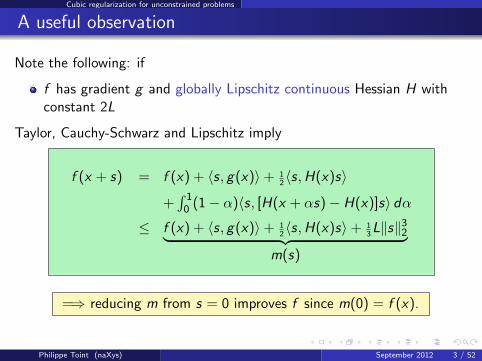
A useful observation
Note the following: if
f has gradient g and globally Lipschitz continuous Hessian H withconstant 2L
Taylor, Cauchy-Schwarz and Lipschitz imply
f (x + s) = f (x) + 〈s, g(x)〉+ 12〈s,H(x)s〉
+∫ 1
0 (1− α)〈s, [H(x + αs)− H(x)]s〉 dα
≤ f (x) + 〈s, g(x)〉+ 12〈s,H(x)s〉+ 1
3L‖s‖3
2︸ ︷︷ ︸m(s)
=⇒ reducing m from s = 0 improves f since m(0) = f (x).
Philippe Toint (naXys) September 2012 3 / 52
Cubic regularization for unconstrained problems
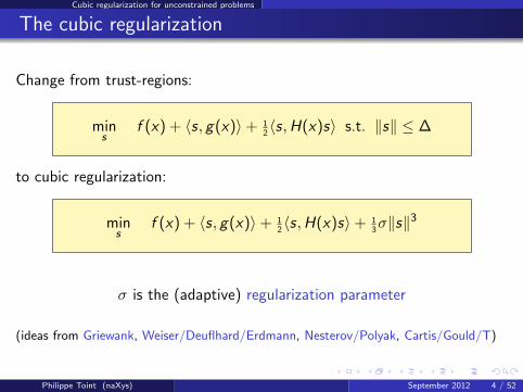
The cubic regularization
Change from trust-regions:
mins
f (x) + 〈s, g(x)〉+ 12〈s,H(x)s〉 s.t. ‖s‖ ≤ ∆
to cubic regularization:
mins
f (x) + 〈s, g(x)〉+ 12〈s,H(x)s〉+ 1
3σ‖s‖3
σ is the (adaptive) regularization parameter
(ideas from Griewank, Weiser/Deuflhard/Erdmann, Nesterov/Polyak, Cartis/Gould/T)
Philippe Toint (naXys) September 2012 4 / 52
Cubic regularization for unconstrained problems
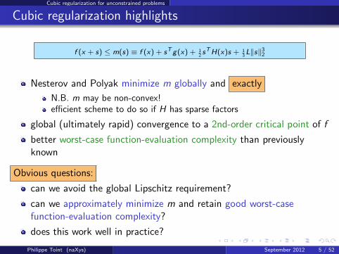
Cubic regularization highlights
f (x + s) ≤ m(s) ≡ f (x) + sT g(x) + 12sTH(x)s + 1
3L‖s‖3
2
Nesterov and Polyak minimize m globally and exactly
N.B. m may be non-convex!efficient scheme to do so if H has sparse factors
global (ultimately rapid) convergence to a 2nd-order critical point of f
better worst-case function-evaluation complexity than previouslyknown
Obvious questions:
can we avoid the global Lipschitz requirement?
can we approximately minimize m and retain good worst-casefunction-evaluation complexity?
does this work well in practice?
Philippe Toint (naXys) September 2012 5 / 52
Cubic regularization for unconstrained problems
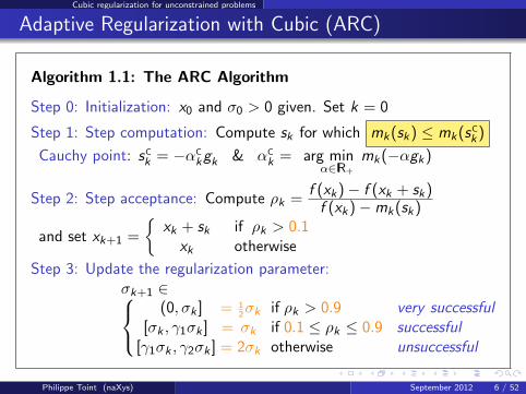
Adaptive Regularization with Cubic (ARC)
Algorithm 1.1: The ARC Algorithm
Step 0: Initialization: x0 and σ0 > 0 given. Set k = 0
Step 1: Step computation: Compute sk for which mk(sk) ≤ mk(sCk)
Cauchy point: sCk = −αC
kgk & αCk = arg min
α∈IR+
mk(−αgk)
Step 2: Step acceptance: Compute ρk =f (xk)− f (xk + sk)f (xk)−mk(sk)
and set xk+1 =
{xk + sk if ρk > 0.1
xk otherwise
Step 3: Update the regularization parameter:σk+1 ∈
(0, σk ] = 12σk if ρk > 0.9 very successful
[σk , γ1σk ] = σk if 0.1 ≤ ρk ≤ 0.9 successful[γ1σk , γ2σk ] = 2σk otherwise unsuccessful
Philippe Toint (naXys) September 2012 6 / 52
Cubic regularization for unconstrained problems
Function-evaluation complexity (1)
How many function evaluations (iterations) are needed to ensure that
‖gk‖ ≤ ε?
So long as for very successful iterations σk+1 ≤ γ3σk for γ3 < 1
The basic ARC algorithm requires at most⌈κCε2
⌉function evaluations
for some κC independent of ε
c.f. steepest descent
Philippe Toint (naXys) September 2012 7 / 52

Cubic regularization for unconstrained problems
Function-evaluation complexity (2)
How many function evaluations (iterations) are needed to ensure that
‖gk‖ ≤ ε?
If H is globally Lipschitz, the s-rule is applied and additionallysk is the global (line) minimizer of mk(αsk) as a function of α,the ARC algorithm requires at most⌈
κSε3/2
⌉function evaluations
for some κS independent of ε.
c.f. Nesterov & PolyakNote: an O(ε−3) bound holds for convergence to second-order criticalpoints.
Philippe Toint (naXys) September 2012 8 / 52

Cubic regularization for unconstrained problems
Function-evaluation complexity (3)
Is the bound in O(ε−3/2) sharp? YES!!!
Construct a unidimensional example with
x0 = 0, xk+1 = xk +
(1
k + 1
) 13
+η
,
f0 =2
3ζ(1 + 3η), fk+1 = fk −
2
3
(1
k + 1
)1+3η
,
gk = −(
1
k + 1
) 23
+2η
, Hk = 0 and σk = 1,
Use Hermite interpolation on [xK , xk+1].
Philippe Toint (naXys) September 2012 9 / 52
Cubic regularization for unconstrained problems
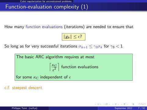
An example of slow ARC (1)
0 1 2 3 4 5 6 7 8 92.222
2.222
2.2221
2.2222
2.2222
2.2222
2.2223x 10
4
The objective function
Philippe Toint (naXys) September 2012 10 / 52
Cubic regularization for unconstrained problems
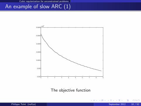
An example of slow ARC (2)
0 1 2 3 4 5 6 7 8 9−1
−0.9
−0.8
−0.7
−0.6
−0.5
−0.4
−0.3
−0.2
−0.1
0
The first derivative
Philippe Toint (naXys) September 2012 11 / 52
Cubic regularization for unconstrained problems
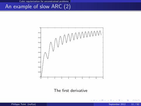
An example of slow ARC (3)
0 1 2 3 4 5 6 7 8 9−1
−0.5
0
0.5
1
1.5
The second derivative
Philippe Toint (naXys) September 2012 12 / 52

Cubic regularization for unconstrained problems
An example of slow ARC (4)
0 1 2 3 4 5 6 7 8 9−10
−5
0
5
10
15
20
The third derivative
Philippe Toint (naXys) September 2012 13 / 52

Cubic regularization for unconstrained problems
Minimizing the model
m(s) ≡ f + sT g + 12sTBs + 1
3σ‖s‖3
2
Small problems:
use More-Sorensen-like method with modified secular equation(also OK as long as factorization is feasible)
Large problems:
an iterative Krylov space method
approximate solution
Numerically sound procedures for computing exact/approximate steps
Philippe Toint (naXys) September 2012 14 / 52
Cubic regularization for unconstrained problems
The main features of adaptive cubic regularization
And the result is. . .
longer steps on ill-conditioned problems
(very satisfactory convergence analysis)
best function-evaluation complexity for nonconvex problems
good performance and reliability
Philippe Toint (naXys) September 2012 15 / 52

Cubic regularization for unconstrained problems
Numerical experience — small problems using Matlab
1 1.5 2 2.5 3 3.5 4 4.5 50
0.1
0.2
0.3
0.4
0.5
0.6
0.7
0.8
0.9
1
α
frac
tion
of p
robl
ems
for
whi
ch m
etho
d w
ithin
α o
f bes
t
Performance Profile: iteration count − 131 CUTEr problems
ACO − g stopping rule (3 failures)ACO − s stopping rule (3 failures)trust−region (8 failures)
Philippe Toint (naXys) September 2012 16 / 52
Unregularized methods
Without regularization ?
What is known for unregularized (standard) methods?
The steepest descent method requires at most⌈κCε2
⌉function evaluations
for obtaining ‖gk‖ ≤ ε.
Sharp???
Newton’s method (when convergent) requires at most
??? function evaluations
for obtaining ‖gk‖ ≤ ε.
Philippe Toint (naXys) September 2012 17 / 52
Unregularized methods
Slow steepest descent (1)
For steepest descent, the bound of⌈κCε2
⌉function evaluations
is sharp on functions with Lipschitz continuous gradients.
As before, construct a unidimensional example with
x0 = 0, xk+1 = xk + αk
(1
k + 1
) 12
+η
,
for some steplength αk > 0 such that
0 < α ≤ αk ≤ α < 2,
giving the step
skdef= xk+1 − xk = αk
(1
k + 1
) 12
+η
.
Philippe Toint (naXys) September 2012 18 / 52
Unregularized methods
Slow steepest descent (1)
Also set
f0 =1
2ζ(1 + 2η), fk+1 = fk − αk(1− 1
2αk)
(1
k + 1
)1+2η
,
gk = −(
1
k + 1
) 12
+η
, and Hk = 1,
Use Hermite interpolation on [xK , xk+1].
Philippe Toint (naXys) September 2012 19 / 52

Unregularized methods
An example of slow steepest descent (1)
0 1 2 3 4 5 6 72.4999
2.4999
2.4999
2.4999
2.4999
2.5
2.5
2.5
2.5
2.5x 10
4
The objective function
Philippe Toint (naXys) September 2012 20 / 52

Unregularized methods
An example of slow steepest-descent (2)
0 1 2 3 4 5 6 7−1
−0.9
−0.8
−0.7
−0.6
−0.5
−0.4
−0.3
−0.2
−0.1
0
The first derivative
Philippe Toint (naXys) September 2012 21 / 52
Unregularized methods
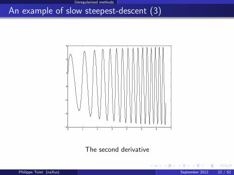
An example of slow steepest-descent (3)
0 1 2 3 4 5 6 7−3
−2
−1
0
1
2
3
The second derivative
Philippe Toint (naXys) September 2012 22 / 52

Unregularized methods
An example of slow steepest descent (4)
0 1 2 3 4 5 6 7−60
−40
−20
0
20
40
60
80
100
The third derivative
Philippe Toint (naXys) September 2012 23 / 52
Unregularized methods
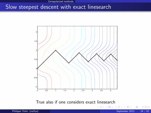
Slow steepest descent with exact linesearch
0 0.5 1 1.5 2 2.5 3 3.5 4
−1
−0.5
0
0.5
1
1.5
2
True also if one considers exact linesearch
Philippe Toint (naXys) September 2012 24 / 52
Unregularized methods
Slow Newton (1)
A big surprise:
Newton’s method may require as much as⌈κCε2
⌉function evaluations
to obtain ‖gk‖ ≤ ε on functions with bounded and (segment-wise) Lipschitz continuous Hessians.
Example now bi-dimensional
Philippe Toint (naXys) September 2012 25 / 52
Unregularized methods
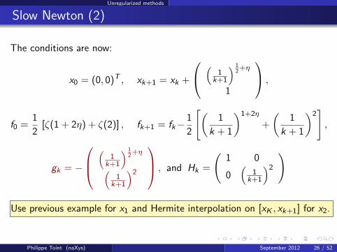
Slow Newton (2)
The conditions are now:
x0 = (0, 0)T , xk+1 = xk +
(1
k+1
) 12
+η
1
,
f0 =1
2[ζ(1 + 2η) + ζ(2)] , fk+1 = fk−
1
2
[(1
k + 1
)1+2η
+
(1
k + 1
)2],
gk = −
(
1k+1
) 12
+η(1
k+1
)2
, and Hk =
(1 0
0(
1k+1
)2
)
Use previous example for x1 and Hermite interpolation on [xK , xk+1] for x2.
Philippe Toint (naXys) September 2012 26 / 52

Unregularized methods
An example of slow Newton
24998.6779
24998.713424998.7134
24998.751924998.7519
24998.7939
24998.7939
24998.8371
24998.8371
24998.888324998.8883
24998.942724998.9427
24998.9427
24999.004824999.0048
24999.0048
24999.07724999.077
24999.077
24999.159324999.1593
24999.159324999.2568
24999.256824999.2568
24999.3789
24999.3789
24999.378924999.3789
24999.535124999.5351
24999.535124999.5351
24999.7591
24999.7591
24999.7591
25000.132125000.1321
25000.13210 1 2 3 4 5 6
0
5
10
15
The path of iterates on the objective’s contours
Philippe Toint (naXys) September 2012 27 / 52

Unregularized methods
More general second-order methods
Assume that, for β ∈ (0, 1], the step is computed by
(Hk + λk I )sk = −gk and 0 ≤ λk ≤ κs‖sk‖β
(ex: Newton, ARC, (TR), . . . )
The corresponding method may require as much as⌈κC
ε−(β+2)/(β+1)
⌉function evaluations
to obtain ‖gk‖ ≤ ε on functions with bounded and (segment-wise) β-Holder continuous Hessians.
Note: ranges form ε−2 to ε−3/2
ARC is optimal within this class
Philippe Toint (naXys) September 2012 28 / 52

Regularization techniques for constrained problems
The constrained case
Can we apply regularization to the constrained case?
Consider the constrained nonlinear programming problem:
minimize f (x)x ∈ F
for x ∈ IRn and f : IRn → IR smooth, and where
F is convex.
Main ideas:
exploit (cheap) projections on convex sets
define using the generalized Cauchy point idea
prove global convergence + function-evaluation complexity
Philippe Toint (naXys) September 2012 29 / 52

Regularization techniques for constrained problems
Constrained step computation (1)
mins
f (x) + 〈s, g(x)〉+ 12〈s,H(x)s〉+ 1
3σ‖s‖3
subject tox + s ∈ F
σ is the (adaptive) regularization parameter
Criticality measure: (as before)
χ(x)def=
∣∣∣∣ minx+d∈F ,‖d‖≤1
〈∇x f (x), d〉∣∣∣∣ ,
Philippe Toint (naXys) September 2012 30 / 52

Regularization techniques for constrained problems
The generalized Cauchy point for ARC
Cauchy step: Goldstein-like piecewise linear seach on mk along thegradient path projected onto F
FindxGCk = PF [xk − tGC
k gk ]def= xk + sGC
k (tGCk > 0)
such that
mk(xGCk ) ≤ f (xk) + κubs〈gk , sGC
k 〉 (below linear approximation)
and either
mk(xGCk ) ≥ f (xk) + κlbs〈gk , sGC
k 〉 (above linear approximation)
or‖PT (xGC
k )[−gk ]‖ ≤ κepp|〈gk , sGCk 〉| (close to path’s end)
no trust-region condition!
Philippe Toint (naXys) September 2012 31 / 52
Regularization techniques for constrained problems
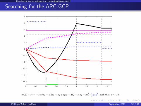
Searching for the ARC-GCP
0 0.2 0.4 0.6 0.8 1 1.2 1.4 1.6
−5
−4
−3
−2
−1
0
1
2
3
4
5
mk (0 + s) = −3.57s1 − 1.5s2 − s3 + s1s2 + 3s22 + s2s3 − 2s2
3 + 13‖s‖3 such that s ≤ 1.5
Philippe Toint (naXys) September 2012 32 / 52
Regularization techniques for constrained problems
A constrained regularized algorithm
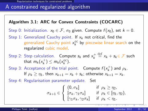
Algorithm 3.1: ARC for Convex Constraints (COCARC)
Step 0: Initialization. x0 ∈ F , σ0 given. Compute f (x0), set k = 0.
Step 1: Generalized Cauchy point. If xk not critical, find thegeneralized Cauchy point xGC
k by piecewise linear search on theregularized cubic model.
Step 2: Step calculation. Compute sk and x+k
def= xk + sk∈ F such
that mk(x+k ) ≤ mk(xGC
k ).
Step 3: Acceptance of the trial point. Compute f (x+k ) and ρk .
If ρk ≥ η1, then xk+1 = xk + sk ; otherwise xk+1 = xk .
Step 4: Regularisation parameter update. Set
σk+1 ∈
(0, σk ] if ρk ≥ η2,[σk , γ1σk ] if ρk ∈ [η1, η2),[γ1σk , γ2σk ] if ρk < η1.
Philippe Toint (naXys) September 2012 33 / 52
Regularization techniques for constrained problems
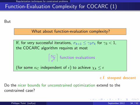
Function-Evaluation Complexity for COCARC (1)
But
What about function-evaluation complexity?
If, for very successful iterations, σk+1 ≤ γ3σk for γ3 < 1,the COCARC algorithm requires at most⌈
κCε2
⌉function evaluations
(for some κC independent of ε) to achieve χk ≤ ε
c.f. steepest descent
Do the nicer bounds for unconstrained optimization extend to theconstrained case?
Philippe Toint (naXys) September 2012 34 / 52

Regularization techniques for constrained problems
Function-evaluation complexity for COCARC (2)
As for unconstrained, impose a termination rule on the subproblemsolution:
Do not terminate solving minxk+s∈F mk(xk + s) before
χmk (x+
k ) ≤ min(κstop, ‖sk‖)χk
where
χmk (x)
def=
∣∣∣∣ minx+d∈F ,‖d‖≤1
〈∇xmk(x), d〉∣∣∣∣
c.f. the “s-rule” for unconstrained
Note: OK at local constrained model minimizers
Philippe Toint (naXys) September 2012 35 / 52
Regularization techniques for constrained problems
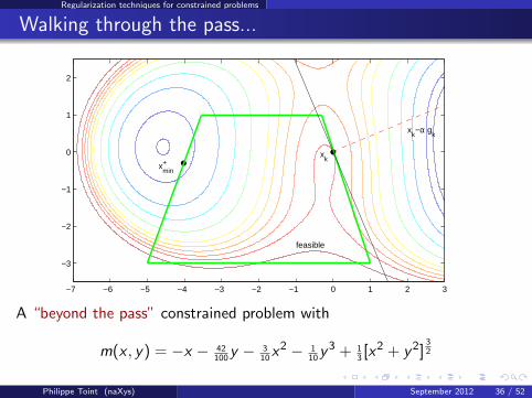
Walking through the pass...
xk
feasible
xk−α g
k
xmin+
−7 −6 −5 −4 −3 −2 −1 0 1 2 3
−3
−2
−1
0
1
2
A “beyond the pass” constrained problem with
m(x , y) = −x − 42100y − 3
10x2 − 1
10y3 + 1
3[x2 + y2]
32
Philippe Toint (naXys) September 2012 36 / 52
Regularization techniques for constrained problems
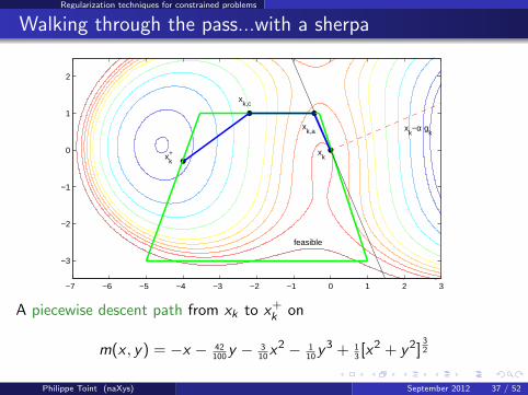
Walking through the pass...with a sherpa
xk
feasible
xk−α g
k
xk+
xk,c
xk,a
−7 −6 −5 −4 −3 −2 −1 0 1 2 3
−3
−2
−1
0
1
2
A piecewise descent path from xk to x+k on
m(x , y) = −x − 42100y − 3
10x2 − 1
10y3 + 1
3[x2 + y2]
32
Philippe Toint (naXys) September 2012 37 / 52
Regularization techniques for constrained problems
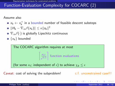
Function-Evaluation Complexity for COCARC (2)
Assume also
xk ← x+k in a bounded number of feasible descent substeps
‖Hk −∇xx f (xk)‖ ≤ κ‖sk‖2
∇xx f (·) is globally Lipschitz continuous
{xk} bounded
The COCARC algorithm requires at most⌈κCε3/2
⌉function evaluations
(for some κC independent of ε) to achieve χk ≤ ε
Caveat: cost of solving the subproblem! c.f. unconstrained case!!!
Philippe Toint (naXys) September 2012 38 / 52
Regularization techniques for constrained problems
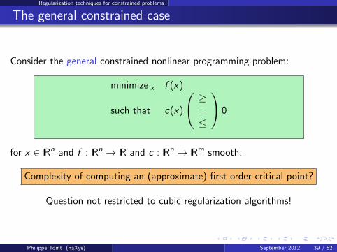
The general constrained case
Consider the general constrained nonlinear programming problem:
minimize x f (x)
such that c(x)
≥=≤
0
for x ∈ IRn and f : IRn → IR and c : IRn → IRm smooth.
Complexity of computing an (approximate) first-order critical point?
Question not restricted to cubic regularization algorithms!
Philippe Toint (naXys) September 2012 39 / 52

Regularization techniques for constrained problems
A detour: minimizing non-smooth composite functions
A useful tool (and an interesting question in itself): consider theunconstrained problem:
minimize x f (x) + h(c(x))
for x ∈ IRn and f : IRn → IR and c : IRn → IRm smooth and nonconvex, andh : IRm → IR non-smooth but convex (ex: h(·) = ‖ · ‖).First-order method: compute a step by solving the (convex) problem
minimize ‖s‖≤∆ `(x , s)def= f (x) + 〈g(x), s〉+ h(c(x) + J(x)s)
for some trust-region radius ∆ (also possible using quadratic regularization)(considered by Nesterov (2007, 2007), Cartis/Gould/T)
Philippe Toint (naXys) September 2012 40 / 52

Regularization techniques for constrained problems
Minimizing non-smooth composite functions (2)
Main result:
Assume f , c and h are globally Lipschitz continuous. Then the“algorithm” takes at most
O(ε−2) function evaluations
to achieveψ(xk) ≤ ε
where ψ(x) is a first-order criticality measure defined by
ψ(x)def= `(x , 0)− min
‖s‖≤1`(x , s).
Philippe Toint (naXys) September 2012 41 / 52
Regularization techniques for constrained problems
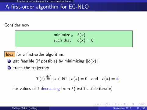
A first-order algorithm for EC-NLO
Consider now
minimize x f (x)such that c(x) = 0
Idea for a first-order algorithm:
1 get feasible (if possible) by minimizing ‖c(x)‖2 track the trajectory
T (t)def= {x ∈ IRn | c(x) = 0 and f (x) = t}
for values of t decreasing from f (first feasible iterate)
Philippe Toint (naXys) September 2012 42 / 52
Regularization techniques for constrained problems
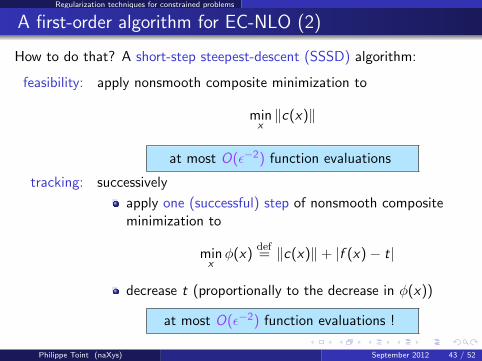
A first-order algorithm for EC-NLO (2)
How to do that? A short-step steepest-descent (SSSD) algorithm:
feasibility: apply nonsmooth composite minimization to
minx‖c(x)‖
at most O(ε−2) function evaluations
tracking: successively
apply one (successful) step of nonsmooth compositeminimization to
minxφ(x)
def= ‖c(x)‖+ |f (x)− t|
decrease t (proportionally to the decrease in φ(x))
at most O(ε−2) function evaluations !
Philippe Toint (naXys) September 2012 43 / 52

Regularization techniques for constrained problems
A view of Algorithm SSSD
Phase 2
Phase 1
Φ(x+,t)
Φ(x,t)
t
t+
ε2 f
||c||
ε−ε
Philippe Toint (naXys) September 2012 44 / 52

Regularization techniques for constrained problems
A complexity result for EC-NLO
Assume f , and c are globally Lipschitz continuous and fbounded below and above in an ε-neighbourhood of feasibil-ity. Then the SSSD algorithm takes at most
O(ε−2) function evaluations
to find an iterate xk with either
‖c(xk)‖ ≤ ε and ‖J(xk)y + gk‖ ≤ ε
for some y , or
‖c(xk)‖ > κfε and ‖J(xk)z‖ ≤ ε
for some z .
(κf ∈ (0, 1), user defined).
Philippe Toint (naXys) September 2012 45 / 52
Regularization techniques for constrained problems
Extensions to the general case
Also applies to inequality constrained problems
by replacing‖c(x)‖ by ‖min(c(x), 0)‖.
Philippe Toint (naXys) September 2012 46 / 52
Regularization techniques for constrained problems
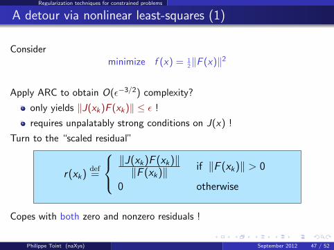
A detour via nonlinear least-squares (1)
Considerminimize f (x) = 1
2‖F (x)‖2
Apply ARC to obtain O(ε−3/2) complexity?
only yields ‖J(xk)F (xk)‖ ≤ ε !
requires unpalatably strong conditions on J(x) !
Turn to the “scaled residual”
r(xk)def=
‖J(xk)F (xk)‖‖F (xk)‖ if ‖F (xk)‖ > 0
0 otherwise
Copes with both zero and nonzero residuals !
Philippe Toint (naXys) September 2012 47 / 52
Regularization techniques for constrained problems
A detour via nonlinear least-squares (2)
Assume f has Lipschitz Hessian. Then the ARC algorithm takesat most
O(ε−3/2) function evaluations
to find an iterate xk with either ‖r(xk)‖ ≤ ε or ‖F (xk)‖ ≤ ε.
No requierement on regularity for J(x) !
Applicable in phase 1 of an algorithm for EC-NLO ?
Philippe Toint (naXys) September 2012 48 / 52
Regularization techniques for constrained problems
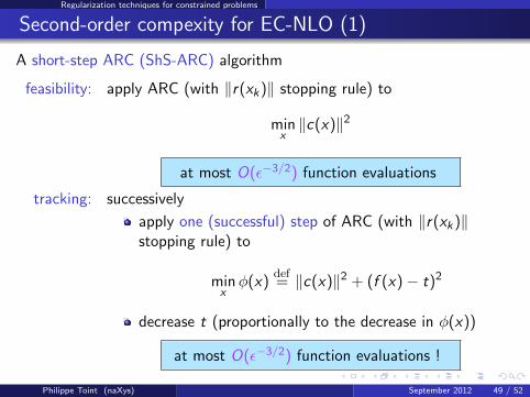
Second-order compexity for EC-NLO (1)
A short-step ARC (ShS-ARC) algorithm
feasibility: apply ARC (with ‖r(xk)‖ stopping rule) to
minx‖c(x)‖2
at most O(ε−3/2) function evaluations
tracking: successively
apply one (successful) step of ARC (with ‖r(xk)‖stopping rule) to
minxφ(x)
def= ‖c(x)‖2 + (f (x)− t)2
decrease t (proportionally to the decrease in φ(x))
at most O(ε−3/2) function evaluations !
Philippe Toint (naXys) September 2012 49 / 52

Regularization techniques for constrained problems
A view of Algorithm ShS-ARC
Phase 2
Phase 1
Φ(x+,t)
Φ(x,t)
t+
t
ε3/2
−ε ε||c||
f
Philippe Toint (naXys) September 2012 50 / 52
Regularization techniques for constrained problems
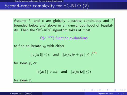
Second-order complexity for EC-NLO (2)
Assume f , and c are globally Lipschitz continuous and fbounded below and above in an ε-neighbourhood of feasibil-ity. Then the ShS-ARC algorithm takes at most
O(ε−3/2) function evaluations
to find an iterate xk with either
‖c(xk)‖ ≤ ε and ‖J(xk)y + gk‖ ≤ ε2/3
for some y , or
‖c(xk)‖ > κfε and ‖J(xk)z‖ ≤ ε
for some z .
Philippe Toint (naXys) September 2012 51 / 52

Conclusions
Conclusions
Many open questions . . . but very interesting
Analysis for unconstrained second-order optimality also possible
Jarre’s example ⇒ global optimization much harder
Algorithm design profits from complexity analysis
Many issues regarding regularizations still unresolved
ARC is optimal amongst second-order method
Many thanks for your attention!
Philippe Toint (naXys) September 2012 52 / 52