evaluation complexity in nonlinear optimization using...
TRANSCRIPT

Evaluation Complexity In Nonlinear OptimizationUsing Lipschitz-Continuous Hessians
Philippe Toint (with Coralia Cartis and Nick Gould)
Namur Center for Complex Systems (naXys), University of Namur, Belgium
Florianopolis, March 2014

Cubic regularization for unconstrained problems
The problem
We consider the unconstrained nonlinear programming problem:
minimize f (x)
for x ∈ IRn and f : IRn → IR smooth.
Important special case: the nonlinear least-squares problem
minimize f (x) = 12‖F (x)‖2
for x ∈ IRn and F : IRn → IRm smooth.
Philippe Toint (naXys)X BRAZOPT,Florianopolis, March 2014 2
/ 41

Cubic regularization for unconstrained problems
A useful observation
Note the following: if
f has gradient g and globally Lipschitz continuous Hessian H withconstant 2L
Taylor, Cauchy-Schwarz and Lipschitz imply
f (x + s) = f (x) + 〈s, g(x)〉+ 12〈s,H(x)s〉
+∫ 10 (1− α)〈s, [H(x + αs)− H(x)]s〉 dα
≤ f (x) + 〈s, g(x)〉+ 12〈s,H(x)s〉+ 1
3L‖s‖32︸ ︷︷ ︸
m(s)
=⇒ reducing m from s = 0 improves f since m(0) = f (x).
Philippe Toint (naXys)X BRAZOPT,Florianopolis, March 2014 3
/ 41

Cubic regularization for unconstrained problems
Approximate model minimization
Lipschitz constant L unknown ⇒ replace by adaptive parameter σk in themodel :
m(s)def= f (x) + sTg(x) + 1
2sTH(x)s + 1
3σk‖s‖32
Computation of the step:
1 minimize m(s) until an approximate first-order minimizer is obtained:
‖∇sm(s)‖ ≤ min[κstop, ‖s‖] ‖gk‖ and ”(before) line minimizer”
(s-rule)Note: no global optimization involved.
Philippe Toint (naXys)X BRAZOPT,Florianopolis, March 2014 4
/ 41

Cubic regularization for unconstrained problems
Adaptive Regularization with Cubic (ARC)
Algorithm 1.1: The ARC2 Algorithm
Step 0: Initialization: x0 and σ0 > 0 given. Set k = 0
Step 1: Step computation: Compute sk for which
‖∇sm(sk)‖ ≤ min[κstop‖sk‖]‖gk‖ and ”(before) line minimizer”
Step 2: Step acceptance: Compute ρk =f (xk)− f (xk + sk)
f (xk)−mk(sk)
and set xk+1 =
{xk + sk if ρk > 0.1
xk otherwise
Step 3: Update the regularization parameter:σk+1 ∈
(0, σk ] = 12σk if ρk > 0.9 very successful
[σk , γ1σk ] = σk if 0.1 ≤ ρk ≤ 0.9 successful[γ1σk , γ2σk ] = 2σk otherwise unsuccessful
Philippe Toint (naXys)X BRAZOPT,Florianopolis, March 2014 5
/ 41

Cubic regularization for unconstrained problems
Cubic regularization highlights
f (x + s) ≤ m(s) ≡ f (x) + sT g(x) + 12sT H(x)s + 1
3L‖s‖32
Nesterov and Polyak minimize m globally and exactly
N.B. m may be non-convex!efficient scheme to do so if H has sparse factors
global (ultimately rapid) convergence to a 2nd-order critical point of f
better worst-case function-evaluation complexity than previouslyknown
Obvious questions:
can we avoid the global Lipschitz requirement? YES!
can we approximately minimize m and retain good worst-casefunction-evaluation complexity? YES !
does this work well in practice? yes
Philippe Toint (naXys)X BRAZOPT,Florianopolis, March 2014 6
/ 41

Cubic regularization for unconstrained problems
Function-evaluation complexity (1)
How many function evaluations (iterations) are needed to ensure that
‖gk‖ ≤ ε?
If H is globally Lipschitz, the s-rule is applied and additionallysk is the global (line) minimizer of mk(αsk) as a function of α,the ARC2 algorithm requires at most⌈
κS
ε3/2
⌉function evaluations
for some κS independent of ε.
c.f. Nesterov & PolyakNote: an O(ε−3) bound holds for convergence to second-order criticalpoints.
Philippe Toint (naXys)X BRAZOPT,Florianopolis, March 2014 7
/ 41
Cubic regularization for unconstrained problems
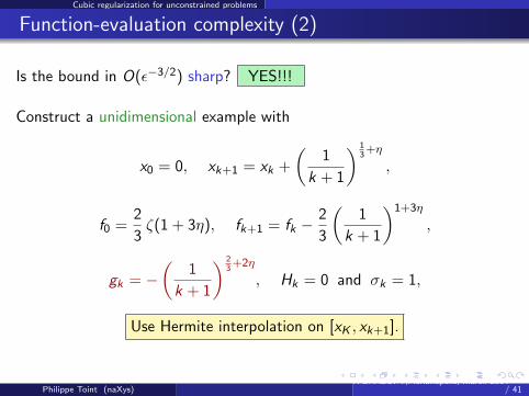
Function-evaluation complexity (2)
Is the bound in O(ε−3/2) sharp? YES!!!
Construct a unidimensional example with
x0 = 0, xk+1 = xk +
(1
k + 1
) 13+η
,
f0 =2
3ζ(1 + 3η), fk+1 = fk −
2
3
(1
k + 1
)1+3η
,
gk = −(
1
k + 1
) 23+2η
, Hk = 0 and σk = 1,
Use Hermite interpolation on [xK , xk+1].
Philippe Toint (naXys)X BRAZOPT,Florianopolis, March 2014 8
/ 41

Cubic regularization for unconstrained problems
An example of slow ARC2 (1)
0 1 2 3 4 5 6 7 8 92.222
2.222
2.2221
2.2222
2.2222
2.2222
2.2223x 10
4
The objective function
Philippe Toint (naXys)X BRAZOPT,Florianopolis, March 2014 9
/ 41

Cubic regularization for unconstrained problems
An example of slow ARC2 (2)
0 1 2 3 4 5 6 7 8 9−1
−0.9
−0.8
−0.7
−0.6
−0.5
−0.4
−0.3
−0.2
−0.1
0
The first derivative
Philippe Toint (naXys)X BRAZOPT,Florianopolis, March 2014 10
/ 41

Cubic regularization for unconstrained problems
An example of slow ARC2 (3)
0 1 2 3 4 5 6 7 8 9−1
−0.5
0
0.5
1
1.5
The second derivative
Philippe Toint (naXys)X BRAZOPT,Florianopolis, March 2014 11
/ 41
Cubic regularization for unconstrained problems
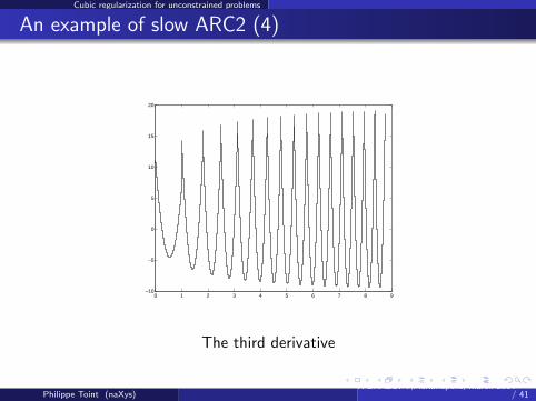
An example of slow ARC2 (4)
0 1 2 3 4 5 6 7 8 9−10
−5
0
5
10
15
20
The third derivative
Philippe Toint (naXys)X BRAZOPT,Florianopolis, March 2014 12
/ 41

Unregularized methods
Slow steepest descent (1)
The steepest descent method with requires at most⌈κC
ε2
⌉function evaluations
for obtaining ‖gk‖ ≤ ε.
NesterovSharp??? YES
Newton’s method (when convergent) requires at most
O(ε−2) function evaluations
for obtaining ‖gk‖ ≤ ε !!!!
Philippe Toint (naXys)X BRAZOPT,Florianopolis, March 2014 13
/ 41

Unregularized methods
Slow Newton (1)
Choose τ ∈ (0, 1)
gk = −
(
1k + 1
) 12+η(
1k + 1
)2
Hk =
(1 0
0(
1k + 1
)2
),
for k ≥ 0 and
f0 = ζ(1+2η)+π2
6, fk = fk−1−
1
2
[(1
k + 1
)1+2η
+
(1
k + 1
)2]
for k ≥ 1,
η = η(τ)def=
τ
4− 2τ=
1
2− τ− 1
2.
Philippe Toint (naXys)X BRAZOPT,Florianopolis, March 2014 14
/ 41

Unregularized methods
Slow Newton (2)
Hksk = −gk ,
and thus
sk =
(
1k + 1
) 12+η
1
,
x0 =
(00
), xk =
k−1∑j=0
(1
j + 1
) 12+η
k
.
Philippe Toint (naXys)X BRAZOPT,Florianopolis, March 2014 15
/ 41

Unregularized methods
Slow Newton (3)
qk(xk+1, yk+1) = fk + 〈gk , sk〉+ 12〈sk ,Hksk〉 = fk+1
0 0.5 1 1.5 2 2.5 3 3.5 4 4.5 50
1
2
3
4
5
6
7
8
9
10
The shape of the successive quadratic modelsPhilippe Toint (naXys)
X BRAZOPT,Florianopolis, March 2014 16/ 41

Unregularized methods
Slow Newton (4)
Define a support function sk(x , y) around (xk , yk)
Philippe Toint (naXys)X BRAZOPT,Florianopolis, March 2014 17
/ 41

Unregularized methods
Slow Newton (5)
A background function fBCK (y) interpolating fk values. . .
0 1 2 3 4 5 6 7 8 9 102.4998
2.4999
2.5
2.5
2.5
2.5001
2.5002x 10⁴
Philippe Toint (naXys)X BRAZOPT,Florianopolis, March 2014 18
/ 41

Unregularized methods
Slow Newton (6)
. . . with bounded third derivative
0 1 2 3 4 5 6 7 8 9 10−20
−15
−10
−5
0
5
Philippe Toint (naXys)X BRAZOPT,Florianopolis, March 2014 19
/ 41
Unregularized methods
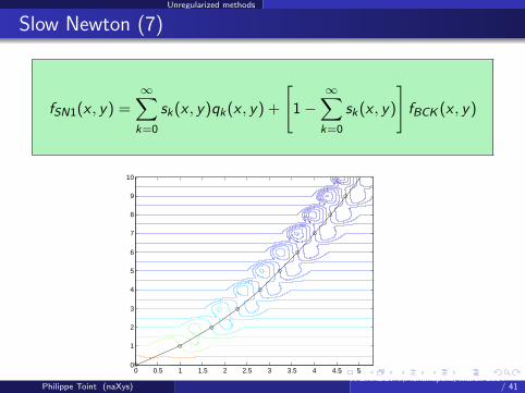
Slow Newton (7)
fSN1(x , y) =∞∑
k=0
sk(x , y)qk(x , y) +
[1−
∞∑k=0
sk(x , y)
]fBCK (x , y)
0 0.5 1 1.5 2 2.5 3 3.5 4 4.5 50
1
2
3
4
5
6
7
8
9
10
Philippe Toint (naXys)X BRAZOPT,Florianopolis, March 2014 20
/ 41

Unregularized methods
Slow Newton (8)
Some steps on a sandy dune. . .
Philippe Toint (naXys)X BRAZOPT,Florianopolis, March 2014 21
/ 41

Unregularized methods
More general second-order methods
Assume that, for β ∈ (0, 1], the step is computed by
(Hk + λk I )sk = −gk and 0 ≤ λk ≤ κs‖sk‖β
(ex: Newton, ARC2, Levenberg-Morrison-Marquardt, (TR2), . . . )
The corresponding method may require as much as⌈κC
ε−(β+2)/(β+1)
⌉function evaluations
to obtain ‖gk‖ ≤ ε on functions with bounded and (segment-wise) β-Holder continuous Hessians.
Note: ranges form ε−2 to ε−3/2
ARC2 is optimal within this class
Philippe Toint (naXys)X BRAZOPT,Florianopolis, March 2014 22
/ 41

Regularization techniques for constrained problems
The constrained case
Can we apply regularization to the constrained case?
Consider the constrained nonlinear programming problem:
minimize f (x)x ∈ F
for x ∈ IRn and f : IRn → IR smooth, and where
F is convex.
Ideas:
exploit (cheap) projections on convex sets
use appropriate termination criterion
χf (xk)def=
∣∣∣∣ minx+d∈F ,‖d‖≤1
〈∇x f (xk), d〉∣∣∣∣ ,
Philippe Toint (naXys)X BRAZOPT,Florianopolis, March 2014 23
/ 41
Regularization techniques for constrained problems
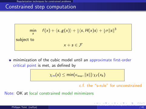
Constrained step computation
mins
f (x) + 〈s, g(x)〉+ 12〈s,H(x)s〉+ 1
3σ‖s‖3
subject tox + s ∈ F
minimization of the cubic model until an approximate first-ordercritical point is met, as defined by
χm(s) ≤ min(κstop, ‖s‖)χf (xk)
c.f. the “s-rule” for unconstrained
Note: OK at local constrained model minimizers
Philippe Toint (naXys)X BRAZOPT,Florianopolis, March 2014 24
/ 41

Regularization techniques for constrained problems
A constrained regularized algorithm
Algorithm 3.1: ARC for Convex Constraints (ARC2CC)
Step 0: Initialization. x0 ∈ F , σ0 given. Compute f (x0), set k = 0.
Step 1: Step calculation. Compute sk and x+k
def= xk + sk∈ F such
that χm(sk) ≤ min(κstop, ‖sk‖)χf (xk).
Step 2: Acceptance of the trial point. Compute f (x+k ) and ρk .
If ρk ≥ η1, then xk+1 = xk + sk ; otherwise xk+1 = xk .
Step 3: Regularisation parameter update. Set
σk+1 ∈
(0, σk ] if ρk ≥ η2,[σk , γ1σk ] if ρk ∈ [η1, η2),[γ1σk , γ2σk ] if ρk < η1.
Philippe Toint (naXys)X BRAZOPT,Florianopolis, March 2014 25
/ 41
Regularization techniques for constrained problems
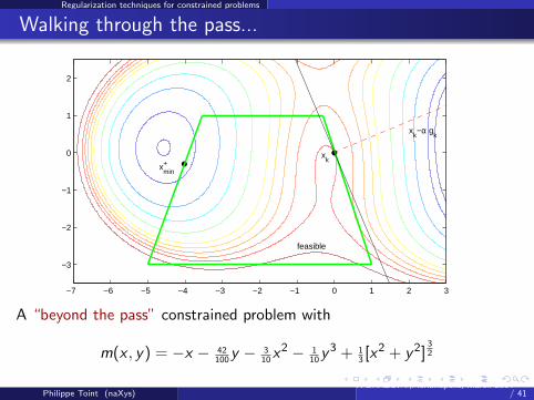
Walking through the pass...
xk
feasible
xk−α g
k
xmin+
−7 −6 −5 −4 −3 −2 −1 0 1 2 3
−3
−2
−1
0
1
2
A “beyond the pass” constrained problem with
m(x , y) = −x − 42100
y − 310
x2 − 110
y3 + 13[x2 + y2]
32
Philippe Toint (naXys)X BRAZOPT,Florianopolis, March 2014 26
/ 41

Regularization techniques for constrained problems
Walking through the pass...with a sherpa
xk
feasible
xk−α g
k
xk+
xk,c
xk,a
−7 −6 −5 −4 −3 −2 −1 0 1 2 3
−3
−2
−1
0
1
2
A piecewise descent path from xk to x+k on
m(x , y) = −x − 42100
y − 310
x2 − 110
y3 + 13[x2 + y2]
32
Philippe Toint (naXys)X BRAZOPT,Florianopolis, March 2014 27
/ 41

Regularization techniques for constrained problems
Function-Evaluation Complexity for ARC2CC
Assume also
xk ← x+k in a bounded number of feasible descent substeps
‖Hk −∇xx f (xk)‖ ≤ κ‖sk‖2
∇xx f (·) is globally Lipschitz continuous
{xk} bounded
The ARC2CC algorithm requires at most⌈κC
ε3/2
⌉function evaluations
(for some κC independent of ε) to achieve χf (xk) ≤ ε
Caveat: cost of solving the subproblem! c.f. unconstrained case!!!
Philippe Toint (naXys)X BRAZOPT,Florianopolis, March 2014 28
/ 41

Regularization techniques for constrained problems
The general constrained case
Consider now the general NLO (slack variables formulation):
minimize x f (x)such that c(x) = 0 and x ∈ F
Ideas for a second-order algorithm:
1 get feasible (if possible) by minimizing ‖c(x)‖2 such that x ∈ F2 track the trajectory
T (t)def= {x ∈ IRn | c(x) = 0 and f (x) = t}
for values of t decreasing from f (first feasible iterate) while preservingx ∈ F
Philippe Toint (naXys)X BRAZOPT,Florianopolis, March 2014 29
/ 41

Regularization techniques for constrained problems
A detour via unconstrained nonlinear least-squares (1)
Considerminimize f (x) = 1
2‖F (x)‖2
Apply ARC2 to obtain O(ε−3/2) complexity?
only yields ‖J(xk)F (xk)‖ ≤ ε !
requires unpalatably strong conditions on J(x) !
Turn to the “scaled residual”
∇x‖F (xk)‖def=
‖J(xk)TF (xk)‖
‖F (xk)‖if ‖F (xk)‖ > 0
0 otherwise
Copes with both zero and nonzero residuals !
Philippe Toint (naXys)X BRAZOPT,Florianopolis, March 2014 30
/ 41

Regularization techniques for constrained problems
A detour via unconstrained nonlinear least-squares (2)
Assume f has Lipschitz Hessian. Then the ARC2 algorithmtakes at most
O(ε−3/2) function evaluations
to find an iterate xk with either
∇x‖F (xk)‖ ≤ ε or ‖F (xk)‖ ≤ ε.
No requirement on regularity for J(x) !
Philippe Toint (naXys)X BRAZOPT,Florianopolis, March 2014 31
/ 41

Regularization techniques for constrained problems
... and via constrained nonlinear least-squares (1)
Consider now
minimize f (x) = 12‖F (x)‖2 such that x ∈ F
Remember termination rules:
χf (xk) ≤ ε (convex inequality constraints)
∇x‖F (xk)‖ ≤ ε (NLSQ)
For inequality-constrained nonlinear least-squares, combine these into
χ‖F (x)‖(xk) =
∣∣∣∣ minx+d∈F ,‖d‖≤1
〈∇x‖F (xk)‖, d〉∣∣∣∣ ≤ ε
Philippe Toint (naXys)X BRAZOPT,Florianopolis, March 2014 32
/ 41

Regularization techniques for constrained problems
... and via constrained nonlinear least-squares (2)
Assume f has Lipschitz Hessian. Then the ARC2CC algorithmtakes at most
O(ε−3/2) function evaluations
to find an iterate xk with either
χ‖F (x)‖(xk) ≤ ε or ‖F (xk)‖ ≤ ε.
Philippe Toint (naXys)X BRAZOPT,Florianopolis, March 2014 33
/ 41

Regularization techniques for constrained problems
Second-order complexity for general NLO (1)
Sketch of a short-step ARC2 (ARC2GC) algorithm
feasibility: apply ARC2CC (with ∇x‖F (xk)‖ stopping rule) to
minx‖c(x)‖2 such that x ∈ F
at most O(ε−3/2) function evaluations
tracking: successively
apply one (successful) step of ARC2CC (with∇x‖F (xk)‖ stopping rule) to
minxφ(x)
def= ‖c(x)‖2 + (f (x)− t)2 such that x ∈ F
decrease t (proportionally to the decrease in φ(x))
at most O(ε−3/2) function evaluations !
Philippe Toint (naXys)X BRAZOPT,Florianopolis, March 2014 34
/ 41
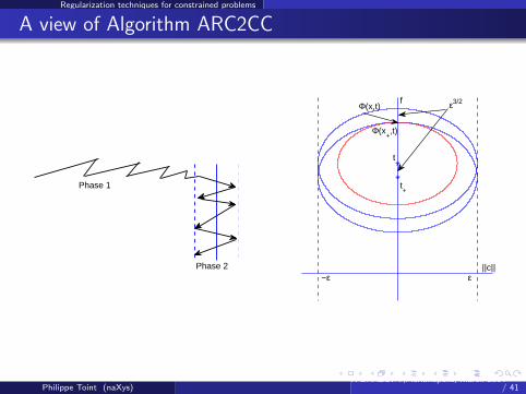
Regularization techniques for constrained problems
A view of Algorithm ARC2CC
Phase 2
Phase 1
Φ(x+,t)
Φ(x,t)
t+
t
ε3/2
−ε ε||c||
f
Philippe Toint (naXys)X BRAZOPT,Florianopolis, March 2014 35
/ 41

Regularization techniques for constrained problems
Second-order complexity for general NLO (2)
Under the “conditions stated above”, the ARC2CC algorithmtakes at most
O(ε−3/2) function evaluations
to find an iterate xk with either
‖c(xk)‖ ≤ δε and χL ≤ ‖(y , 1)‖ε2/3
for some Lagrange multiplier y and where
L(x , y) = f (x) + 〈y , c(x)〉,
or‖c(xk)‖ > δε and χ||c|| ≤ ε.
Philippe Toint (naXys)X BRAZOPT,Florianopolis, March 2014 36
/ 41

Conclusions
Conclusions
Complexity analysis for first-order critical points using second-ordermethods complete !
O(ε−3/2) (unconstrained, general constraints !)
Available also for first order methods :
O(ε−2) (unconstrained, general constraints !)
Jarre’s example ⇒ global optimization much harder
smooth functions littered with approximate critical points !
ARC2 is optimal amongst second-order method
More also known (unconstrained 2nd order criticality, DFO, etc)
Many thanks for your attention!
Philippe Toint (naXys)X BRAZOPT,Florianopolis, March 2014 37
/ 41