Working Paper 09-46 Departamento de Economía Economic Series (25) Universidad Carlos III de Madrid May 2009 Calle Madrid, 126 28903 Getafe (Spain) Fax (34) 916249875

Evaluating Value-at-Risk models via Quantile

Regression Wagner Piazza Gaglianone∗ Luiz Renato Lima† Oliver Linton‡ Daniel Smith§

14th May 2009

Abstract This paper is concerned with evaluating value at risk estimates. It is well known that using

only binary variables, such as whether or not there was an exception, sacrifices too much information. However, most of the specification tests (also called backtests) available in the literature, such as Christoffersen (1998) and Engle and Maganelli (2004) are based on such variables. In this paper we propose a new backtest that does not rely solely on binary variables. It is shown that the new backtest provides a sufficient condition to assess the finite sample performance of a quantile model whereas the existing ones do not. The proposed methodology allows us to identify periods of an increased risk exposure based on a quantile regression model (Koenker & Xiao, 2002). Our theoretical findings are corroborated through a Monte Carlo simulation and an empirical exercise with daily S&P500 time series. Keywords: Value-at-Risk, Backtesting, Quantile Regression. JEL Classification: C12, C14, C52, G11.

∗ Research Department, Central Bank of Brazil (e-mail: wagner.gaglianone@bcb.gov.br). † Corresponding author. Department of Economics, University of Illinois and Graduate School of Economics,

Getulio Vargas Foundation, Praia de Botafogo 190, s.1104, Rio de Janeiro, RJ 22.253-900, Brazil (e-mail: luizr@fgv.br). ‡ Department of Economics, London School of Economics, Houghton Street, London WC2A 2AE, United Kingdom

(e-mail: o.linton@lse.ac.uk). § Faculty of Business Administration, Simon Fraser University, 8888 University Drive, Burnaby BC V6P 2T8,

Canada (e-mail: drsmith@sfu.ca).

1 Introduction

Recent �nancial disasters have emphasized the need for accurate risk measures for �nancial institu-

tions. Value-at-Risk (VaR) models were developed in response to the �nancial disasters of the early

90s, and have become a standard measure of market risk, which is increasingly used by �nancial

and non-�nancial �rms as well. In fact, VaR is a statistical risk measure of potential losses, and

summarizes in a single number the maximum expected loss over a target horizon, at a particular

signi�cance level. Despite several other competing risk measures proposed in the literature, VaR

has e¤ectively become the cornerstone of internal risk management systems in �nancial institutions,

following the success of the J.P. Morgan (1996) RiskMetrics system, and nowadays form the basis

of the determination of market risk capital, since the 1996 Amendment of the Basel Accord.

Another advantage of VaR is that it can be seen as a coherent risk measure for a large class

of continuous distributions, that is, it satis�es the following properties: (i) subadditivity (the risk

measure of a portfolio cannot be greater than the sum of the risk measures of the smaller portfolios

that comprise it); (ii) homogeneity (the risk measure is proportional to the scale of the portfolio);

(iii) monotonicity (if portfolio Y dominates X, in the sense that each payo¤ of Y is at least as large

as the corresponding payo¤ of X, i.e., X � Y , then X must be of lesser or equal risk) and; (iv)

risk free condition (adding a risk-free instrument to a portfolio decreases the risk by the size of the

investment in the risk-free instrument).

Daníelsson et al. (2005) and Ibragimov and Walden (2007) show that for continuous random

variables either VaR is coherent and satis�es subadditivity or the �rst moment of the investigated

variable does not exist. In this sense, they show that VaR is subadditive for the tails of all fat

distributions, provided the tails are not super fat (e.g., Cauchy distribution). In this way, for a

very large class of distributions of continuous random variables, one does not have to worry about

subadditivity violations for a VaR risk measure.

A crucial issue that arises in this context is how to evaluate the performance of a VaR model.

According to Giacomini and Komunjer (2005), when several risk forecasts are available, it is desir-

able to have formal testing procedures for comparison, which do not necessarily require knowledge

of the underlying model, or, if the model is known, do not restrict attention to a speci�c estimation

procedure. The literature has proposed several tests (also known as "backtests"), such as Kupiec

(1995), Christo¤ersen (1998) and Engle and Manganelli (2004), mainly based on binary variables

(i.e., an indicator for whether the loss exceeded the VaR), from which statistical properties are de-

rived and further tested. More recently, Berkowitz et al. (2009) developed a uni�ed framework for

VaR evaluation and showed that the existing backtests can be interpreted as a Lagrange Multiplier

(LM) type of tests.

2

The existing backtests are based on orthogonality conditions between a binary variable and

some instruments. If the VaR model is correctly speci�ed, then this orthogonality condition holds

and one can therefore use it to derive an LM test. Monte carlo simulations have shown that such

tests have low power in �nite samples against a variety of misspeci�ed models. The problem arises

because binary variables are constructed to represent rare events. In �nite samples, it may be

the case that there are few extreme events, leading to a lack of the information needed to reject

a misspeci�ed model. In this case, a typical solution would be to either increase the sample size

or construct a new test that uses more information than the existing ones to reject a misspeci�ed

model.

The contribution of this paper is twofold. First we propose a random coe¢ cient model that

can be used to construct a Wald test for the null hypothesis that a given VaR model is correctly

speci�ed. To the best of our knowledge, no such framework exists in the current literature. It is well

known that although LM and Wald tests are asymptotically equivalent under the null hypothesis

and local alternatives, they can yield quite di¤erent results in �nite samples. We show in this paper

that the new test uses more information to reject a misspeci�ed model which makes it deliver more

power in �nite samples than any other existing test.

Another limitation of the existing tests is that they do not give any guidance as to how the VaR

models are wrong. The second contribution of this paper is to develop a mechanism by which we

can evaluate the local and global performance of a given VaR model and, therefore, �nd out why

and when it is misspeci�ed. By doing this, we can unmask the reasons of rejection of a misspeci�ed

model. This information could be used to reveal if a given model is under or over estimating risk,

if it reacts quickly to increases in volatility, or even to suggest possible model combinations that

would result in more accurate VaR estimates. Indeed, it has been proven that model combination

(see Issler and Lima, 2009) can increase the accuracy of forecasts. Since VaR is simply a conditional

quantile, it is also possible that model combination can improve the forecast of a given conditional

quantile or even of an entire density.

Our Monte Carlo simulations as well as our empirical application using the S&P500 series

corroborate our theoretical �ndings. Moreover, the proposed test is quite simple to compute and

can be carried out using software available for conventional quantile regression, and is applicable

even when the VaR does not come from a conditional volatility model.

This study is organized as follows: Section 2 de�nes Value-at-Risk and the model we use,

section 3 presents a quantile regression-based hypothesis test to evaluate VaRs. In Section 4,

we brie�y describe the existing backtests and establish a su¢ cient condition to assess a quantile

model. Section 5 shows the Monte Carlo simulation comparing the size and power of the competing

backtests. Section 6 provides an empirical exercise based on daily S&P500 series, and Section 7

3

concludes.

2 The Model

A Value-at-Risk model reports the maximum loss that can be expected, at a particular signi�cance

level, over a given trading horizon. If Rt denotes return of a portfolio at time t, and �� 2 (0; 1)denotes a (pre-determined) signi�cance level, then the respective VaR (Vt) is implicitly de�ned by

the following expression:

Pr [Rt < VtjFt�1] = ��; (1)

where Ft�1 is the information set available at time t� 1. From the above de�nition, it is clear that

Vt is the ��th conditional quantile of Rt. In other words, Vt is the one-step ahead forecast of the

��th quantile of Rt based on the information available up to period t� 1.From Equation (1) it is clear that �nding a VaR is equivalent to �nding the conditional quantile

of Rt. Following the idea of Christo¤ersen et al. (2001), one can think of generating a VaR measure

as the outcome of a quantile regression, treating volatility as a regressor. In this sense, Engle and

Patton (2001) argue that a volatility model is typically used to forecast the absolute magnitude

of returns, but it may also be used to predict quantiles. In this paper, we adapt the idea of

Christo¤ersen et al. (2001) to investigate the accuracy of a given VaR model. In particular, instead

of using the conditional volatility as a regressor, we simply use the VaR measure of interest (Vt).

We embed this measure in a general class of models for stock returns in which the speci�cation

that delivered Vt is nested as a special case. In this way, we can provide a test of the VaR model

through a conventional hypothesis test. Speci�cally, we consider that there is a random coe¢ cient

model for Rt, generated in the following way:

Rt = �0(Ut) + �1(Ut)Vt (2)

= x0t�(Ut); (3)

where Vt is Ft�1-measurable in the sense that it is already known at period t, Ut � iid U(0; 1),

and �i(Ut), i = 0; 1 are assumed to be comonotonic in Ut, with �(Ut) = [�0(Ut); �1 (Ut)]0 and

x0t = [1; Vt].

Proposition 1 Given the random coe¢ cient model (2) and the comonotonicity assumption of

�i(Ut), i = 0; 1, the �th conditional quantile of Rt can be written as

QRt (� j Ft�1) = �0(�) + �1 (�)Vt ; for all � 2 (0; 1): (4)

Proof. See appendix.

4

Now, recall what we really want to test: Pr (Rt � Vt j Ft�1) = ��, that is, Vt is indeed the ��th

conditional quantile of Rt. Therefore, considering the conditional quantile model (4), a natural way

to test for the overall performance of a VaR model is to test the null hypothesis

Ho :

(�0(�

�) = 0

�1 (��) = 1

(5)

against the general alternative.

The null hypothesis can be presented in a classical formulation as Ho :W�(��) = r, for the �xed

signi�cance level (quantile) � = ��, where W is a 2 � 2 identity matrix; �(��) = [�0(��); �1 (��)]0

and r = [0; 1]. Note that, due to the simplicity of our restrictions, the latter null hypothesis can

still be reformulated as Ho : �(��) = 0, where �(��) = [�0(��); (�1(��)� 1)]0. Notice that the nullhypothesis should be interpreted as a Mincer and Zarnowitz (1969) type-regression framework for

a conditional quantile model.

3 The Test Statistic and Its Null Distribution

Let b�(��) be the quantile regression estimator of �(��): The asymptotic distribution of b�(��) canbe derived following Koenker (2005, p.74), and it is normal with covariance matrix that takes the

form of a Huber (1967) sandwich:pT (b�(��)� �(��)) d! N(0; ��(1� ��)H�1

�� JH�1�� ) = N(0;���); (6)

where J = p limT!1

1T

TPt=1

xtx0t and H�� = p lim

T!11T

TPt=1

xtx0t[ft(QRt(�

�jxt)] under the quantile regression

model QRt(� j xt) = x0t�(�). The term ft(QRt(��jxt) represents the conditional density of Rt

evaluated at the quantile ��. Consistent estimators of J and H�� are computed by using, for

instance, the techniques in Koenker and Machado (1999). Given that we are able to compute the

covariance matrix of the estimated b�(�) coe¢ cients, we can now construct our hypothesis test toverify the performance of the Value-at-Risk model based on quantile regressions (hereafter, VQR

test).

De�nition 1: Let our test statistic be de�ned by

�V QR = T [b�(��)0(��(1� ��)H�1�� JH

�1�� )

�1b�(��)]: (7)

In addition, consider the following assumptions:

Assumption 1: Let xt be measurable with respect to Ft�1 and zt � fRt; xtg be a strictly station-ary process;

5

Assumption 2: (Density) Let Rt have conditional (on xt) distribution functions Ft, with continu-

ous Lebesgue densities ft uniformly bounded away from 0 and 1 at the points QRt(� j xt) =F�1t (� j xt) for all � 2 (0; 1);

Assumption 3: (Design) There exist positive de�nite matrices J and H� , such that for all � 2(0; 1):

J = p limT!1

1

T

TPt=1

xtx0t ; H� = p lim

T!1

1

T

TPt=1

xtx0t[ft(QRt(� j xt))]:

Assumption 4: maxi=1;:::;T kxik =pT

p! 0.

The asymptotic distribution of the VQR test statistic, under the null hypothesis thatQRt (�� j Ft�1) =

Vt, is given by Proposition 1 below, which is merely an application of Hendricks and Koenker (1992)

and Koenker (2005, Theorem 4.1) for a �xed quantile ��.

Proposition 2 (VQR test) Consider the quantile regression (4). Under the null hypothesis (5),

if assumptions (1)-(4) hold, then, the test statistic �V QR is asymptotically chi-squared distributed

with two degrees of freedom.

Proof. See appendix.

Remark 1: Assumption (1) together with comonotonicity of �i(Ut), i = 0; 1 guarantee the

monotonic property of the conditional quantiles. We recall the comment of Robinson (2006), in

which the author argues that comonotonicity may not be su¢ cient to ensure monotonic conditional

quantiles, in cases where xt can assume negative values. In our case, xt � 0: Assumption (2) relaxesthe iid assumption in the sense that it allows for non-identical distributions. Bounding the quantile

function estimator away from 0 and 1 is necessary to avoid technical complications. Assumptions

(2)-(4) are quite standard in the quantile regression literature (e.g., Koenker and Machado (1999)

and Koenker and Xiao (2002)) and familiar throughout the literature on M-estimators for regression

models, and are crucial to apply the CLT of Koenker (2005, Theorem 4.1).

Remark 2: Under the null hypothesis it follows that Vt = QRt (�� j Ft�1), but under the

alternative hypothesis the random nature of Vt, captured in our model by the estimated coe¢ cientsb�(��) 6= 0, can be represented by Vt = QRt (�� j Ft�1) + �t, where �t represents the measurement

error of the VaR on estimating the latent variableQRt (�� j Ft�1). Note that assumptions (1)-(4) are

easily satis�ed under the null and the alternative hypotheses. In particular, note that assumption

(4) under H1 implies that also �t is bounded.

6

Remark 3: Assumptions (1)-(4) do not restrict our methodology to those cases in which Vtis constructed from a conditional volatility model. Indeed, our methodology can be applied to a

broad number of situations, such as:

(i) The model used to construct Vt is known. For instance, a risk manager trying to construct

a reliable VaR measure. In such a case, it is possible that: (ia) Vt is generated from a conditional

volatility model, e.g., Vt = g(b�2t ), where g(�) is some function of the estimated conditional varianceb�2t , say from a GARCH model; or (ib) Vt is directly generated, for instance, from a CAViaR model

or an ARCH-quantile method (See Koenker & Zhao (1996) and Wu & Xiao (2002) for further

details);

(ii) Vt is generated from an unknown model, and the only information available is fRt; Vtg. Inthis case, we are still able to apply Proposition 1 as long as assumptions (1)-(4) hold. This might

be the case described in Berkowitz and O�Brien (2002), in which a regulator investigates the VaR

measure reported by a supervised �nancial institution;

(iii) Vt is generated from an unknown model, but besides fRt; Vtg a con�dence interval of Vt isalso reported. Suppose that a sequence fRt; Vt; V t; V tg is known, in which Pr

�V t < Vt < V t j Ft�1

�=

�, where [V t; V t] are respectively lower and upper bounds of Vt, generated (for instance) from a

bootstrap procedure, with a con�dence level � (see Christo¤ersen and Goncalves (2005), Hartz et.

al. (2006) and Pascual et al. (2006)). One could use this additional information to investigate the

considered VaR by making a connection between the con�dence interval of Vt and the previously

mentioned measurement error �t. The details of this route remain an issue to be further explored.

4 Existing Backtests

Recall that a correctly speci�ed VaR model at level �� is nothing other than the ��th conditional

quantile of Rt. The goal of the econometrician is to test the null hypothesis that Vt correctly

approximates the conditional quantile for a speci�ed level ��. In this section, we review some of

the existing backtests, which are based on an orthogonality condition between a binary variable

and some instruments. This framework is the basis of GMM estimation and o¤ers a natural way to

construct a Lagrange Multiplier (LM) test. Indeed, the current literature on backtesting is mostly

represented by LM type of tests. In �nite samples, the LM test and the Wald test proposed in this

paper can perform quite di¤erent. In particular, we will show that the test proposed in this paper

consider more information than some of the existing test and, therefore, it can deliver more power

in �nite sample.

7

We �rst de�ne a violation sequence by the following indicator function or hit sequence:

Ht =

(1 ; if Rt < Vt

0 ; if Rt � Vt: (8)

By de�nition, the probability of violating the VaR should always be

Pr(Ht = 1jFt�1) = ��: (9)

Based on these de�nitions, we now present some backtests usually mentioned in the literature to

identify misspeci�ed VaR models:

(i) Kupiec (1995): Some of the earliest proposed VaR backtests is due to Kupiec (1995),

which proposes a nonparametric test based on the proportion of exceptions. Assume a sample size

of T observations and a number of violations of N =TPt=1Ht. The objective of the test is to know

whether bp � N=T is statistically equal to ��:

Ho : p = E(Ht) = ��: (10)

The probability of observing N violations over a sample size of T is driven by a Binomial

distribution and the null hypothesis Ho : p = �� can be veri�ed through a LR test (also known as

the unconditional coverage test). This test rejects the null hypothesis of an accurate VaR if the

actual fraction of VaR violations in a sample is statistically di¤erent than ��. However, Kupiec

(1995) �nds that the power of his test is generally low in �nite samples, and the test becomes more

powerful only when the number of observations is very large.

(ii) Christo¤ersen (1998): The unconditional coverage property does not give any informa-

tion about the temporal dependence of violations, and the Kupiec (1995) test ignores conditioning

coverage, since violations could cluster over time, which should also invalidate a VaR model. In

this sense, Christo¤ersen (1998) extends the previous LR statistic to specify that the hit sequence

should also be independent over time. The author argues that we should not be able to predict

whether the VaR will be violated, since if we could predict it, then, that information could be used

to construct a better risk model. The proposed test statistic is based on the mentioned hit sequence

Ht, and on Tij that is de�ned as the number of days in which a state j occurred in one day, while

it was at state i the previous day. The test statistic also depends on �i, which is de�ned as the

probability of observing a violation, conditional on state i the previous day. It is also assumed that

the hit sequence follows a �rst order Markov sequence with transition matrix given by

� =

Previous day"1� �0 1� �1�0 �1

#current day (violation)

no violation(11)

8

Note that under the null hypothesis of independence, we have that � = �0 = �1 = (T01 + T11)=T ,

and the following LR statistic can, thus, be constructed:

LRind: = 2 ln

(1� �0)T00�T010 (1� �1)T10�T111(1� �)(T00+T10)�(T01+T11)

!: (12)

The joint test, also known as the �conditional coverage test�, includes the unconditional coverage

and independence properties. An interesting feature of this test is that a rejection of the conditional

coverage may suggest the need for improvements on the VaR model, in order to eliminate the

clustering behavior. On the other hand, the proposed test has a restrictive feature, since it only

takes into account the autocorrelation of order 1 in the hit sequence.

Berkowitz et al (2009) extended and uni�ed the existing tests by noting that the de-meaned

violations Hitt = Ht � �� form a martingale di¤erence sequence (m.d.s.). By the de�nition of the

violation, equations (8) and (9) imply that

E[HittjFt�1] = 0,

that is, the de-meaned violations form an m.d.s. with respect to Ft�1. This implies that Hitt isuncorrelated at all leads and lags. In other words, for any vector Xt in Ft�1 we must have

E[Hitt Xt] = 0; (13)

which constitutes the basis of GMM estimation. The framework based on such orthogonality

conditions o¤ers a natural way to construct a Lagrange Multiplier (LM) test. Indeed, if we allow

Xt to include lags of Hitt, Vt and its lags, then we obtain the well-known DQ test proposed by

Engle and Manganelli (2004), which we describe below.

(iii) Engle & Manganelli (2004) proposed a new test that incorporates a variety of alternatives.

Using the previous notation, the random variable Hitt = Ht��� is de�ned by the authors, in orderto construct the dynamic conditional quantile (DQ) test, which involves the following statistic:

DQ = (Hit0tXt[X0tXt]

�1X 0tHitt)=(T�(1� �)); (14)

where the vector of instruments Xt might include lags of Hitt, Vt and its lags). This way, Engle

& Manganelli (2004) test the null hypothesis that Hitt and Xt are orthogonal. Under their null

hypothesis, the proposed test statistic follows a �2q , in which q = rank(Xt). Note that the DQ

test can be used to evaluate the performance of any type of VaR methodology (and not only the

CAViaR family, proposed in their paper).

Several other related procedures can be immediately derived from the orthogonality condition

(13). For example, Chirsto¤ersen and Pelletier (2004) and Haas (2005) propose duration-based

9

tests to the problem of assessing VaR accuracy. However, as shown by the Monte-carlo experiment

in Berkowitz et. al. (2009), the DQ test in which Xt = Vt appears to be the best backtest for

1% VaR models, and other backtests generally have much lower power against misspeci�ed VaR

models. In the next section, we provide a link between the proposed VQR test and the DQ test,

and we give some reasons that suggest the VQR test should be more powerful than the DQ test in

�nite samples.

4.1 DQ versus VQR test

In the previous section we showed that the DQ test proposed by Engle and Manganelli (2004)

can be interpreted as a LM test. The orthogonality condition (13) constitutes the basis of GMM

estimation and therefore can be used to estimate the quantile regression model (4) under the null

hypothesis (5). It is well know that OLS and GMM are asymptotically equivalent. By analogy,

quantile regression estimation and GMM estimation are also known to be asymptotically equivalent

(see for instance, footnote 5 of Buchinsky, 1998, and the proofs of Powell, 1984). However, if the

orthogonality condition (13) provides a poor �nite-sample approximation of the objective function,

then GMM and quantile regression estimation will be quite di¤erent and the LM tests and Wald test

proposed in this paper will yield very di¤erent results. In order to compare the DQ test and our VQR

test, we consider the simplest case in which Xt = [1 Vt]0. As showed in Koenker (2005, pp. 32-37),

the quantile regression estimator minimizes the objective function R(�) =Pnt=1 �� (yt � x0t� (�)),

where �� (u) = �u1(u � 0) + (� � 1)u1(u < 0). Notice that �� is piecewise linear and continuousfunction, and it is di¤erentiable except at the points at which one or more residuals are zero. At

such points, R(�) has directional derivatives in all directions. The directional derivative of R in

direction w (OR(�;w)) is given by OR(�;w) =�Pnt=1 (yt � x0t�;�x0tw)x0tw, where

(u; v) =

(� � I(u < 0), if u 6= 0� � I(v < 0), if u = 0:

If at point �0, OR(�0; w) > 0 for all w 2 Rp with kwk = 1, then �0 minimizes R(�). Now, considerthe quantile problem which the VQR is based on. Therein, if we set yt = Rt, xt = [1 Vt]

0 and

�0 = [0 1]0, then the directional derivative becomes OR(�0; w)=�Pnt=1 (yt � x0t�0;�x0tw)x0tw,

where

�yt � x0t�0;�x0tw

�x0tw =

(Hitt [1 Vt]w, if ut 6= 0Hit�tx

0tw, if ut = 0;

and Hit�t = I([1 Vt]w < 0) � � . Notice that the function Hit is the same one de�ned by Engle

and Manganelli (2004) and that Hitt 6= Hit�t . According to Koenker (2005), there will be at least

10

p zero residuals where p is the dimension of �. This suggests that the orthogonality condition

n�1Pnt=1Hitt [1 Vt] = 0, does not imply OR(�0; w) > 0 for all w 2 R2 with kwk = 1. In this

case, the orthogonality condition is not su¢ cient to assess a performance of a quantile model Vt in

�nite samples. In practice, the VQR test is using more information than the DQ test to reject a

misspeci�ed model and, therefore, it can exhibit superior power in �nite samples than the DQ test.

Finally, it is possible to generalize this result for a list of instruments larger than Xt = [1 Vt]0 as

long as we rede�ne our quantile regression (4) to include other regressors besides an intercept and

Vt

Although the �rst order condition n�1Pnt=1Hitt [1 Vt] = 0 does not strictly imply in the optim-

ality condition OR(�0; w) > 0 in �nite samples, this does not prevent it from holding asymptoticallyif one makes an assumption that the number of zero residuals are op(1) (see the discussion in the

handbook chapter of Newey and McFadden (1994). Hence, the DQ test proposed by Engle and

Manganelli and our VQR test are asymptotically equivalent under the null hypothesis and local

alternatives. However, in �nite samples the orthogonality and the optimality conditions can be

quite di¤erent and the two tests can therefore yield very di¤erent results

Finally, notice that if OR(�0; w) > 0 for all w 2 R2 with kwk = 1; then n�1Pnt=1Hitt [1 Vt] = 0.

Therefore, the DQ test is implied by the VQR when the VaR model is correctly speci�ed. Intuitively

this happens because if Vt = QRt(�� j Ft�1), then Vt will provide a �lter to transform a (possibly)

serially correlated and heteroskedastic time series into a serially independent sequence of indicator

functions.

In sum, the above results suggest that there are some reasons to prefer the VQR test over the

DQ test since the former can have more power in �nite sample and be equivalent to the latter

under the null hypothesis. A small Monte Carlo simulation is conducted in Section 4 to verify these

theoretical �ndings as well as to compare the VQR test with the existing ones in terms of power

and size.

5 Monte Carlo simulation

In this section we conduct a simulation experiment to investigate the �nite sample properties of the

VQR test. In particular we are interested in showing under which conditions our theoretical �ndings

are observed in �nite samples. We consider, besides the VQR test, the unconditional coverage test

of Kupiec (1995), the conditional coverage test of Christo¤ersen (1998) and the out-of-sample DQ

test of Engle and Manganelli (2004), in which we considered the instruments Xt = [1 Vt]0. We look

at the one-day ahead forecast and simulate 5,000 sample paths of length T +Te observations, using

the �rst Te = 250 observations to compute the initial values of (18) with T = f250; 500; 1000; 2500g

11

(i.e., approximately 1, 2, 4, and 10 years of daily data).

Asymptotic critical values are used in this monte carlo experiment, but bootstrap methods

could also be considered to compute �nite-sample critical values. For example, for the VQR test

we could have employed the bootstrap method proposed by Parzen et al (1994). For the Kupiec,

Christor¤ersen and DQ tests, �nite-sample critical values could be computed by using the method

proposed by Dufour (2006). Bootstrap based critical values are more di¢ cult to be computed by

a �nancial institution on a daily basis. On the other hand, asymptotic critical values may not be

accurate enough in small samples. As the results in this section show, asymptotic critical values

are reasonably accurate for sample size of 4 years of daily observations, which is not a restriction

for many �nancial institutions.

Nonetheless, the lack of accuracy in asymptotic critical values can give rise to size distortions

especially for samples as small as T = 250. In order to avoid that these size distortions favor some

tests in terms of power, we will compute the so called size-adjusted power. In the size-adjusted

power, the 5% critical value is going to correspond to the 5% quantile of the test statistic distribution

under the null hypothesis. In doing this, we eliminate any power performance of tests caused by

the use of asymptotic critical values. Of course, if the empirical size is close to the nominal one,

which is 5%, then size-adjusted and asymptotic power will be close to each other as well.

We start evaluating the empirical size of 5% tests. To assess the size of the tests we will

assume that the correct data-generating process is a zero mean, unit unconditional variance normal

innovation-based GARCH model:

Rt = �t"t; t = 1; :::; T , (15)

�2t = (1� �� �) + � � y2t�1 + � � �2t�1; (16)

where � = 0:05 and � = 0:90, and "t � iidN(0; 1). We therefore compute the true VaR as

Vt = �t��1�� (17)

where ��1�� denotes the �� quantile of a standard normal random variable. Since we are computing

5% tests, we should expect that under the null hypothesis each test would reject the correctly

speci�ed model Vt = �t��1�� 5% of times.

Table 1 reports the size of tests for �� = 1% and �� = 5%, one can see that the asymptotic

critical values do not do a good job when �� = 1% and sample size as small as T = 250. In this

case there are few observations around the 1% quantile of Rt implying an inaccurate estimation of

QRt(0:01 j Ft�1). The VQR test responds to it by rejecting the null model more frequently than5% of the time. However, we can see that if we allow for larger samples, the empirical size of the

12

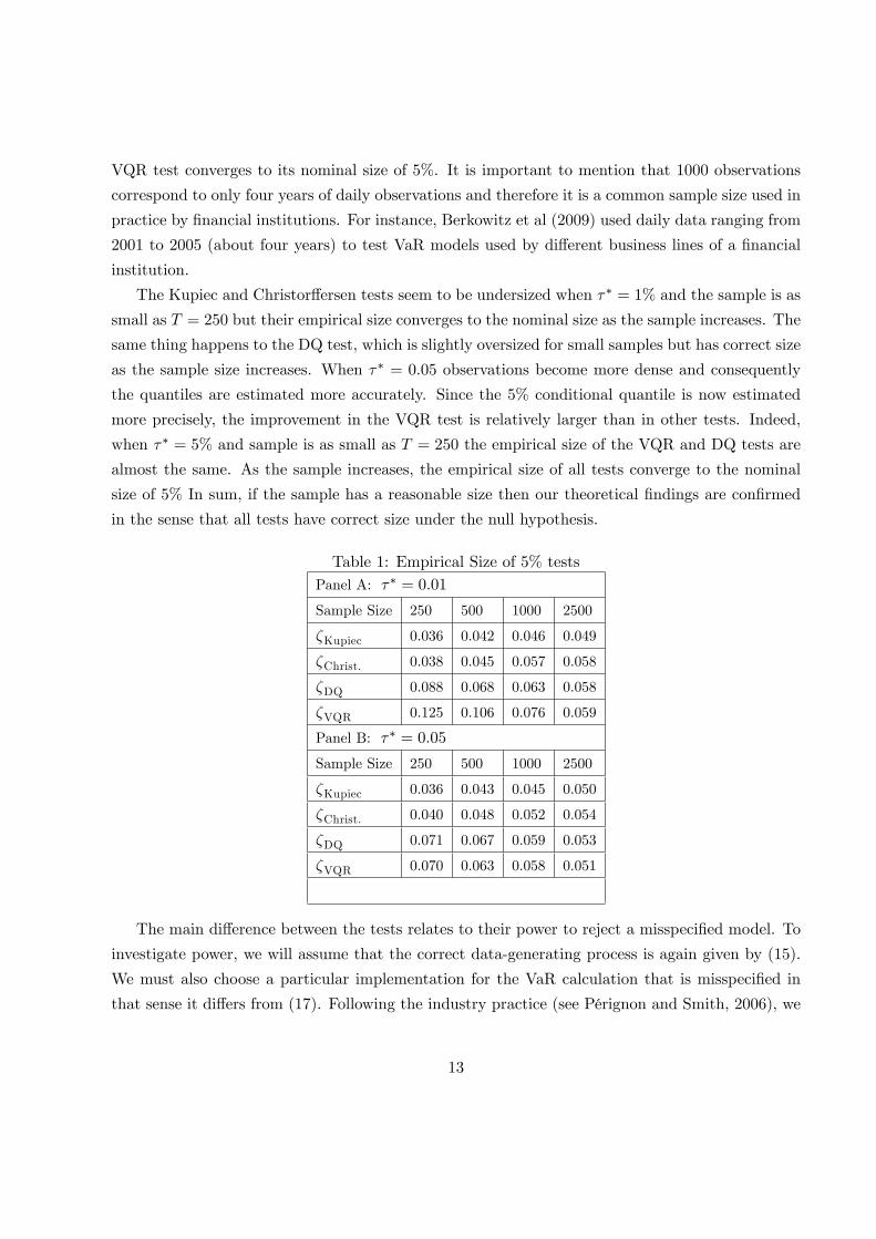
VQR test converges to its nominal size of 5%. It is important to mention that 1000 observations

correspond to only four years of daily observations and therefore it is a common sample size used in

practice by �nancial institutions. For instance, Berkowitz et al (2009) used daily data ranging from

2001 to 2005 (about four years) to test VaR models used by di¤erent business lines of a �nancial

institution.

The Kupiec and Christor¤ersen tests seem to be undersized when �� = 1% and the sample is as

small as T = 250 but their empirical size converges to the nominal size as the sample increases. The

same thing happens to the DQ test, which is slightly oversized for small samples but has correct size

as the sample size increases. When �� = 0:05 observations become more dense and consequently

the quantiles are estimated more accurately. Since the 5% conditional quantile is now estimated

more precisely, the improvement in the VQR test is relatively larger than in other tests. Indeed,

when �� = 5% and sample is as small as T = 250 the empirical size of the VQR and DQ tests are

almost the same. As the sample increases, the empirical size of all tests converge to the nominal

size of 5% In sum, if the sample has a reasonable size then our theoretical �ndings are con�rmed

in the sense that all tests have correct size under the null hypothesis.

Table 1: Empirical Size of 5% testsPanel A: �� = 0:01

Sample Size 250 500 1000 2500

�Kupiec 0.036 0.042 0.046 0.049

�Christ. 0.038 0.045 0.057 0.058

�DQ 0.088 0.068 0.063 0.058

�VQR 0.125 0.106 0.076 0.059

Panel B: �� = 0:05

Sample Size 250 500 1000 2500

�Kupiec 0.036 0.043 0.045 0.050

�Christ. 0.040 0.048 0.052 0.054

�DQ 0.071 0.067 0.059 0.053

�VQR 0.070 0.063 0.058 0.051

The main di¤erence between the tests relates to their power to reject a misspeci�ed model. To

investigate power, we will assume that the correct data-generating process is again given by (15).

We must also choose a particular implementation for the VaR calculation that is misspeci�ed in

that sense it di¤ers from (17). Following the industry practice (see Pérignon and Smith, 2006), we

13

assume that the Bank uses an 1-year Historical Simulation method to compute its VaR. Speci�cally,

Vt = percentile�fRsgts=t�Te ; 100�

�� . (18)

Historical simulation is by far the most most popular VaR model used by commercial banks.

Indeed, Pérignon and Smith (2006) document that almost three-quarters of banks that disclose

their VaR method report using historical simulation. Historical simulation is the empirical quantile

and therefore does not respond well to increases in volatility (see Pritsker, 2001). Combining its

popularity and this weakness it is the natural choice for the misspeci�ed VaR Model (we note that

Berkowitz, Christor¤ersen, and Pelletier, 2006, use a similar experiment).

Table 2 reports the size-adjusted power. When �� = 1% and the sample size is as small as

250, all tests present low power against the misspeci�ed historical simulation model. Even in this

situation, the VQR test is more powerful than any other test. When the sample size increases,

the VQR test becomes even more powerful against the historical simulation model rejecting such

a misspeci�ed model 17%, 49% and 80% of the times when T = 500; 1000 and 2500, respectively.

This performance is by far the best one among all backtests considered in this paper. The Kupiec

test rejects the misspeci�ed model only 32,2% of the times when T = 2500, which is close to the

rate of the Christor¤ersen test (39,6%), but below the DQ test (64,4%). If a model is misspeci�ed,

then a backtest is supposed to use all available information to reject it. The Kupiec test has

low power because it ignores the information about the time dependence of the hit process. The

conditional coverage tests (Christor¤ersen and DQ) sacri�ce information that comes from zero

residuals and therefore fail to reject a misspeci�ed model when the orthogonality condition holds,

but the optimality condition does not. The VQR test simply compares the empirical conditional

quantiles that is estimated from the data with the conditional quantile estimated by using the

historical simulation model. If these two estimates are very di¤erent from each other, then the null

hypothesis is going to be rejected and the power of the test is delivered.

There are theoretically few observations below Vt when �� = 1%, which explains the low power

exhibited by all tests. When �� = 5% the number of observations below Vt increases, giving to

the tests more information that can be used to reject a misspeci�ed model. Hence, we expect

that the power of each test will increase when one considers �� = 5% rather than �� = 1%. This

additional information is used di¤erently by each test. Here again the VQR bene�ts from using

more information than any other test to reject a misspeci�ed model. Indeed, even for T = 250 the

VQR rejects the null hypothesis 21,5% of the times, above Kupiec (6,8%), Christor¤ersen (14,2%)

and DQ (17,9%) test. For T = 2500 the power of the VQR approaches 90% against 42,3%, 50,9%

and 76,9% for Kupiec, Chistor¤ersen and DQ respectively.

14

Table 2: Size-adjusted Power of 5% testsPanel A: �� = 1%

Sample Size 250 500 1000 2500

�Kupiec 0.059 0.113 0.189 0.322

�Christ. 0.087 0.137 0.216 0.396

�DQ 0.084 0.171 0.402 0.644

�VQR 0.091 0.174 0.487 0.800

Panel B: �� = 5%

Sample Size 250 500 1000 2500

�Kupiec 0.068 0.146 0.267 0.423

�Christ. 0.142 0.227 0.319 0.509

�DQ 0.179 0.316 0.454 0.769

�VQR 0.215 0.366 0.644 0.883

Another advantage of the random coe¢ cient framework proposed in this paper is that it can be

used to derive a statistical device that indicates why and when a given VaR model is misspeci�ed.

In the next section we introduce this device and show how to use it to identify periods of risk

exposure.

6 Local analysis of VaR models: identifying periods of risk expos-

ure

The conditional coverage literature is concerned with the adequacy of the VaR model, in respect

to the existence of clustered violations. In this section, we will take an alternative route to analyze

the conditional behavior of a VaR measure. According to Engle and Manganelli (2004), a good

Value-at-Risk model should produce a sequence of unbiased and uncorrelated hits, and any noise

introduced into the Value-at-Risk measure would change the conditional probability of a hit vis-à-

vis the related VaR. Given that our study is entirely based on a quantile framework, besides the

VQR test, we are also able to identify the exact periods in which the VaR produces an increased

risk exposure in respect to its nominal level ��, which is quite a novelty in the literature. To do so,

let us �rst introduce some notation:

De�nition 2: Wt � fQUt(e�) = e� 2 [0; 1] j Vt = QRt (e� j Ft�1)g, representing the empiricalquantile of the standard iid uniform random variable, Ut, such that the equality Vt =

QRt (e� j Ft�1) holds at period t.15

In other words, Wt is obtained by comparing Vt with a full range of estimated conditional

quantiles evaluated at � 2 [0; 1]. Note that Wt enables us to conduct a local analysis, whereas

the proposed VQR test is designed for a global evaluation based on the whole sample. It is worth

mentioning that, based on our assumptions, QRt (� j Ft�1) is monotone increasing in � , and Wt by

de�nition is equivalent to a quantile level, i.e., Wt > �� , QRt (Wt j Ft�1) > QRt (�� j Ft�1). Also

note that if Vt is a correctly speci�ed VaR model, then Wt should be as close as possible to �� for

all t. However, if Vt is misspeci�ed, then it will vague away from ��, suggesting that Vt does not

correctly approximate the ��th conditional quantile.

Notice that, due to the quantile regression setup, one does not need to know the true returns

distribution in order to constructWt. In practical terms, based on the series Rt; Vt one can estimate

the conditional quantile functions QRt (� j Ft�1) for a (discrete) grid of quantiles � 2 [0; 1]. Then,one can construct Wt by simply comparing (in each time period t) the VaR series Vt with the set

of estimated conditional quantile functions QRt (� j Ft�1) across all quantiles � inside the adoptedgrid.

Now consider the set of all observations = 1; : : : ; T , in which T is the sample size, and de�ne

the following partitions of :

De�nition 3: H � ft 2 j Wt > ��g, representing the periods in which the VaR belongs to aquantile above the level of interest �� (indicating a conservative model);

De�nition 4: L � ft 2 j Wt < ��g, representing the periods in which the VaR is below thenominal �� level and, thus, underestimate the risk in comparison to ��.

Since we partitioned the set of periods into two categories, i.e. = H + L, we can now

properly identify the so-called periods of "risk exposure" L. Let us summarize the previous

concepts through the following schematic graph:

Figure 1 - Periods of risk exposure

16

It should be mentioned that a VaR model that exhibits a good performance in the VQR test

(i.e., in which Ho is not rejected) is expected to exhibit Wt as close as possible to ��, �uctuating

around ��, in which periods of Wt below �� are balanced by periods above this threshold. On the

other hand, a VaR model rejected by the VQR test should present a Wt series detached from ��,

revealing the periods in which the model is conservative or underestimate risk. This additional

information can be extremely useful to improve the performance of the underlying Value-at-Risk

model, since the periods of risk exposure are now easily revealed.

7 Empirical exercise

7.1 Data

In this section, we explore the empirical relevance of the theoretical results previously derived. This

is done by evaluating and comparing two VaR models, based on the VQR test and other competing

backtests commonly presented in the literature. To do so, we investigate the daily returns of

S&P500 over the last 4 years, with an amount of T = 1000 observations, depicted in the following

�gure:

Figure 2 - S&P500 daily returns (%)

­3.00%

­2.00%

­1.00%

0.00%

1.00%

2.00%

3.00%

Oct­03 Aug­04 May­05 Mar­06 Jan­07 Nov­070

40

80

120

160

200

240

­0.025 0.000 0.025

Series: SP500Sample 1 1000Observations 1000

Mean  0.000416Median  0.000788Maximum  0.028790Minimum ­0.035343Std. Dev.  0.007140Skewness ­0.253716Kurtosis  4.553871

Jarque­Bera  111.3334Probability  0.000000

Notes: a) The sample covers the period from 23/10/2003 until 12/10/2007;

b) Source: Yahoo!Finance.

Note from the graph and the summary statistics the presence of common stylized facts about

�nancial data (e.g., volatility clustering; mean reverting; skewed distribution; excess kurtosis ; and

non-normality, see Engle and Patton, 2001, for further details). The two Value-at-Risk models ad-

opted in our evaluation procedure are the popular 12-months historical simulation (HS12M) and the

GARCH (1,1) model. According to Perignon and Smith (2006) about 75% of �nancial institutions

in the US, Canada and Europe that disclose their VaR model report using historical simulation

methods. The choice of a GARCH (1,1) model with Gaussian innovations is motivated by the work

of Berkowitz and O0Brien (2002) who documented that the performance of the GARCH(1,1) is

highly accurate even as compared to more sophisticated structural models.

17

In addition, recall that we are testing the null hypothesis that the model Vt correctly approx-

imates the true ��th conditional quantile of the return series Rt. We are not testing the null

hypothesis that Vt correctly approximates the entire distribution of Rt. Therefore, it is possible

that for di¤erent ��s (target probabilities) the model Vt might do well at a target probability, but

otherwise poorly (see Kuester et al., 2005).

Practice generally shows that di¤erent models lead to widely di¤erent VaR time series for the

same considered return series, leading us to the crucial issue of model comparison and hypothesis

testing. The HS12M method has serious drawbacks and is expected to generate poor VaR measures,

since it ignores the dynamic ordering of observations, and volatility measures look like "plateaus",

due to the so-called "ghost e¤ect". On the other hand, as shown by Christo¤ersen et al. (2001),

the GARCH-VaR model is the only VaR measure, among several alternatives considered by the

authors, which passes the Christo¤ersen�s (1998) conditional coverage test.

7.2 Results

We start by showing the local analysis results for each VaR model. When �� = 1 �gure 3 shows that

the VaR computed by the HS12M method is above the 1% line most of the times, indicating that

such a model over estimate 1% VaR very frequently. The same does not happen to the GARCH(1,1)

model, which seems to yield VaR estimates that are very close to the 1% line. If we now turn our

attention to the 5% value-at-risk, we can see that both models have a poor performance. Indeed,

The VaR estimated from the HS12M model seems to be quite erratic, with some periods in which

1% VaR is under estimated and other periods in which it is over estimated. The GARCH(1,1)

model seems to under estimate 1% VaR most of the times, although it does not seem to yield a

VaR estimate that is far below 0.03. Therefore, if we backtest these two models. we should expect to

reject the 1% VaR estimated by HS12M, and the 5% VaR estimated by HS12M and GARCH(1,1).

The results from our backtesting is exhibited in Table 3. Note that this local behavior investigation

could only be conducted through our proposed quantile regression methodology, which we believe

to be a novelty in the backtest literature.

18

Figure 3 - Local Analysis of VaR Models.

HS12m - 1% VaR GARCH - 1% VaR

0.00

0.01

0.02

0.03

0.04

0.05

0.06

0.07

0.08

0.09

0.10

1 101 201 301 401 501 601 701 801 9010.00

0.01

0.02

0.03

0.04

0.05

0.06

0.07

0.08

0.09

0.10

1 101 201 301 401 501 601 701 801 901

HS12m - 5% VaR GARCH - 5% VaR

0.00

0.01

0.02

0.03

0.04

0.05

0.06

0.07

0.08

0.09

0.10

1 101 201 301 401 501 601 701 801 9010.00

0.01

0.02

0.03

0.04

0.05

0.06

0.07

0.08

0.09

0.10

1 101 201 301 401 501 601 701 801 901

Despite its poor local performance, the HS12M model is not rejected by Kupiec and Christof-

fersen tests at 5% level of signi�cance. In part, this can explained by the fact that the Kupiec test

is mainly concerned on the percentage of hits generated by the VaR model, which in the case of

the HS12M model reported in table 3, does not seem to be far away from the hypothetical levels

The null hypothesis of the Christo¤ersen test is very restrictive, being rejected when there is strong

evidence against �rst order dependence of the hit function or when the percentage of hits is far away

from ��. It is well known that there many other forms of time dependence that is not accounted by

the null hypothesis of the Christo¤ersen test. The more powerful test of Engle and Manganelli with

the ex-ante VaR as the only instrument performs quite well and rejects the misspeci�ed HS12M

model for �� = 1% and 5%. As expected, the VQR test performs quite well, easily rejecting the

misspeci�ed HS12M.

In our local analysis, the GARCH (1,1) model seems to work well when we use it to estimate

a 1% VaR but fails to estimate a 5% VaR accurately. The backtest analysis in Table 3 indicates

that neither tests rejects the null hypothesis that the GARCH(1,1) is a correctly speci�ed model

for a 1% VaR. However, as documented by Kuester et al. (2005) it is possible that for di¤erent

���s (target probabilities) the model can do well at a given target probability, but otherwise poorly

at another target probability. Here, the GARCH(1,1) model seems to predict the 1% VaR quite

19

well but not the 5% VaR. However, when we backtest the GARCH(1,1) for �� = 5% by using the

existing backtests, we fail to reject the null hypothesis. This results suggest that the GARCH(1,1)

model correctly predicts the 5% VaR despite the clear evidence against it showed in Figure 3. The

results of Table 3 indicate that GARCH(1,1) model for the 5% VaR is only rejected by the VQR

test, which is compatible with the previous evidence in �gure 3. Our methodology is, therefore,

able to reject more misspeci�ed VaR models in comparison to other backtests.

Table 3: Backtesting Value-at-Risk ModelsModel % of Hits �Kupiec �Christ. �DQ �VQR

�� = 1%

HS12M 1.6 0.080 0.110 0.000 0.000

GARCH(1,1) 1.1 0.749 0.841 0.185 0.010

�� = 5%

HS12M 5.5 0.466 0.084 0.000 0.000

GARCH(1,1) 4.5 0.470 0.615 0.841 0.042

Notes: P-values are shown in the ��s columns

8 Conclusions

Backtesting could prove very helpful in assessing Value-at-Risk models and is nowadays a key

component for both regulators and risk managers. Since the �rst procedures suggested by Kupiec

(1995) and Christo¤ersen (1998), a lot of research has been done in the search for adequate meth-

odologies to assess and help improve the performance of VaRs, which (preferable) do not require

the knowledge of the underlying model.

As noted by the Basle Committee (1996), the magnitude as well as the number of exceptions of a

VaR model is a matter of concern. The so-called "conditional coverage" tests indirectly investigate

the VaR accuracy, based on a "�ltering" of a serially correlated and heteroskedastic time series

(Rt) into a serially independent sequence of indicator functions (hit sequence Hitt). Thus, the

standard procedure in the literature is to verify whether the hit sequence is iid. However, an

important piece of information might be lost in that process, since the conditional distribution of

returns is dynamically updated. This issue is also discussed by Campbell (2005), which states that

the reported quantile provides a quantitative and continuous measure of the magnitude of realized

pro�ts and losses, while the hit indicator only signals whether a particular threshold was exceeded.

In this sense, the author suggests that quantile tests can provide additional power to detect an

inaccurate risk model.

20

That is exactly the objective of this paper: to provide a VaR-backtest fully based on a quantile

regression framework. Our proposed methodology enables us to: (i) formally conduct a Wald-type

hypothesis test to evaluate the performance of VaRs; and (ii) identify periods of an increased risk

exposure. We illustrate the usefulness of our setup through an empirical exercise with daily S&P500

returns, in which we construct �ve competing VaR models and evaluate them through our proposed

backtest (and through other standard backtests).

Since a Value-at-Risk model is implicitly de�ned as a conditional quantile function, the quantile

approach provides a natural environment to study and investigate VaRs. One of the advantages of

our approach is the increased power of the suggested quantile-regression backtest in comparison to

some established backtests in the literature, as suggested by a Monte Carlo simulation. Perhaps

most importantly, our backtest is applicable under a wide variety of structures, since it does not

depend on the underlying VaR model, covering either cases where the VaR comes from a conditional

volatility model, or it is directly constructed (e.g., CAViaR or ARCH-quantile methods) without

relying on a conditional volatility model. We also introduce a main innovation: based on the

quantile estimation, one can also identify periods in which the VaR model might increase the risk

exposure, which is a key issue to improve the risk model, and probably a novelty in the literature.

A �nal advantage is that our approach can easily be computed through standard quantile regression

softwares.

Although the proposed methodology has several appealing properties, it should be viewed as

complementary rather than competing with the existing approaches, due to the limitations of the

quantile regression technique discussed along this paper. Furthermore, several important topics

remain for future research, such as: (i) time aggregation: how to compute and properly evaluate a

10-day regulatory VaR? Risk models constructed through QAR (Quantile Autoregressive) technique

can be quite promising due to the possibility of recursively generation of multiperiod density forecast

(see Koenker and Xiao (2006a,b)); (ii) Our randomness approach of VaR also deserves an extended

treatment and leaves room for weaker conditions; (iii) multivariate VaR: although the extension of

the analysis for the multivariate quantile regression is not straightforward, several proposals have

already been suggested in the literature (see Chaudhuri (1996) and Laine (2001)); (iv) inclusion of

other variables to increase the power of VQR test in other directions; (v) improvement of the BIS

formula for market required capital; (vi) nonlinear quantile regressions; among many others.

According to the Basel Committee (2006), new approaches to backtesting are still being de-

veloped and discussed within the broader risk management community. At present, di¤erent banks

perform di¤erent types of backtesting comparisons, and the standards of interpretation also di¤er

21

somewhat across banks. Active e¤orts to improve and re�ne the methods currently in use are un-

derway, with the goal of distinguishing more sharply between accurate and inaccurate risk models.

We aim to contribute to the current debate by providing a quantile technique that can be useful

as a valuable diagnostic tool, as well as a mean to search for possible model improvements.

Acknowledgements

We would like to thank the Joint Editor Arthur Lewbel, an anonymous Associate Editor, two anonymous

referees, Ignacio Lobato, Richard Smith, J.C. Escanciano and Keith Knight for their helpful comments and

suggestions. Lima would like to thank CNPq for �nancial support as well as the University of Illinois. Linton

would like to thank the ESRC and Leverhulme foundations for �nancial support as well as the Universidad

Carlos III de Madrid-Banco Santander Chair of Excellence.

Appendix A. Proofs of Propositions

Proof of Proposition 1. Given the random coe¢ cient model (2), we can compute the con-

ditional quantile of Rt as QRt (� j Ft�1) = Q[�0(Ut)+�1(Ut)V aRt] (� j Ft�1). Comonotonicity impliesthat QPp

i=1�i(Ut)

=Ppi=1Q�i(Ut). Therefore we can write QRt (� j Ft�1) = Q�0(Ut) (� j Ft�1) +

Q�1(Ut)V aRt (� j Ft�1). Since �i (Ut) are increasing functions of the iid standard uniform random

variable Ut, then we know that Q�i(Ut) = �i(QUt) and therefore QRt (� j Ft�1) = �0 (QUt(�)) +

�1 (QUt(�))V aRt. Finally, recall that Ut � iid U(0; 1) and therefore QUt(�) = � , � 2 (0; 1). whichimplies QRt (� j Ft�1) = �0 (�) + �1 (�)V aRt, � 2 (0; 1).

Proof of Proposition 2. By Assumption (1), we have that the conditional quantile function

is monotone increasing in � , which is a crucial property of Value-at-Risk models. In other words,

we have that QRt (�1 j Ft�1) < QRt (�2 j Ft�1) for all �1 < �2 2 (0; 1). Assumptions (2)-(4)

are regularity conditions necessary to de�ne the asymptotic covariance matrix, and a continuous

conditional quantile function, needed for the CLT (6) of Koenker (2005, Theorem 4.1). A sketch of

the proof of this CLT, via a Bahadur representation, is also presented in Hendricks and Koenker

(1992, Appendix). Given that we established the conditions for the CLT (6), our proof is concluded

by using standard results on quadratic forms: For a given random variable z � N(�;�) it follows

that (z��)0��1(z��) � �2r where r = rank(�). See Johnson and Kotz (1970, p. 150) and White

(1984, Theorem 4.31) for further details.

22

References

[1] Artzner, P., Delbaen, F., Eber, J.-M., Heath, D. (1999), "Coherent Measures of Risk." Mathematical

Finance 9, 203-228.

[2] Basle Committee on Banking Supervision. (1996), "Amendment to the Capital Accord to Incorporate

Market Risks," BIS - Bank of International Settlements.

[3] Berkowitz, J., O�Brien, J. (2002), "How Accurate are the Value-at-Risk Models at Commercial Banks?"

Journal of Finance 57, 1093-1111.

[4] Berkowitz, J., Christo¤ersen, P., Pelletier, D. (2009), "Evaluating Value-at-Risk Models with Desk-

Level Data", forthcoming in Management Science.

[5] Buchinsky, M. (1998), "Recent Advances in Quantily Regression Models: A Practical Guideline for

Empirical Research," The Journal of Human Resources, 33, 88-126.

[6] Campbell, S.D. (2005), "A Review of Backtesting and Backtesting Procedures," Finance and Economics

Discussion Series, Working Paper 21.

[7] Charles, A., Darné, O. (2005), "Outliers and GARCH models in �nancial data," Economic Letters 86,

347-352.

[8] Chaudhuri, P. (1996), "On a geometric notion of quantiles for multivariate data," Journal of the Amer-

ican Statistical Association 91, 862-872.

[9] Chen, J.E. (2001), "Investigations on Quantile Regression: Theories and Applications for Time Series

Models," National Chung-Cheng University, mimeo.

[10] Chen, M.Y., Chen, J.E. (2002), "Application of Quantile Regression to Estimation of Value at Risk,"

National Chung-Cheng University, mimeo.

[11] Chernozhukov, V., Umantsev, L. (2001), "Conditional Value-at-Risk: Aspects of Modelling and Estim-

ation," Empirical Economics 26 (1), 271-292.

[12] Christo¤ersen, P.F. (1998), "Evaluating interval forecasts," International Economic Review 39, 841-862.

[13] ______ (2003), "Elements of Financial Risk Management," San Diego: Academic Press.

[14] Christo¤ersen, P.F., Goncalves, S. (2005), "Estimation Risk in Financial Risk Management," Journal

of Risk 7, 1�28.

23

[15] Christo¤ersen, P.F., Hahn, J., Inoue, A. (2001), "Testing and Comparing Value-at-Risk Measures,"

Journal of Empirical Finance 8, 325-342.

[16] Christo¤ersen, P.F., Pelletier, D. (2004), "Backtesting Value-at-Risk: A Duration-Based Approach,"

Journal of Financial Econometrics 2 (1), 84-108.

[17] Crnkovic, C., Drachman, J. (1997), "Quality Control in VaR: Understanding and Applying Value-at-

Risk," London: Risk Publications.

[18] Daníelsson, J., de Vries, C. (1997),. "Tail index and quantile estimation with very high frequency data,"

Journal of Empirical Finance 4, 241-257.

[19] Daníelsson, J., Jorgensen, B.N., Samorodnitsky, G., Sarma, M., de Vries, C.G. (2005), "Suadditivity

Re-examined: the case for Value-at-Risk," Manuscript. London School of Economics. Downloaded from

www.RiskResearch.org.

[20] Dowd, K. (2005), "Measuring Market Risk," John Wiley and Sons Ltd., 2nd edition.

[21] Embrechts, P., Kluppelberg, C., Mikosch, T. (1997), "Modelling Extremal Events," Springer-Verlag.

[22] Embrechts, P., Resnick, Samorodnitsky, G. (1999), "Extreme value theory as a risk management tool,"

North American Actuarial Journal 3, 30-41.

[23] Engle, R.F. (1982), "Autoregressive Conditional Heteroskedasticity with Estimates of the Variance of

U.K. In�ation," Econometrica 50, 987-1008.

[24] Engle, R.F., Manganelli, S. (2004),." CAViaR: Conditional Autoregressive Value at Risk by Regression

Quantiles," Journal of Business and Economic Statistics 22 (4), 367-381.

[25] Engle, R.F., Patton, A.J. (2001), "What good is a volatility model?" Quantitative Finance, Institute

of Physics Publishing 1, 237�245.

[26] Franses, P.H., Ghijsels, H. (1999), "Additive outliers, GARCH and forecasting volatility," International

Journal of Forecasting 15, 1-9.

[27] Giacomini, R., Komunjer, I. (2005), "Evaluation and Combination of Conditional Quantile Forecasts,"

Journal of Business and Economic Statistics 23 (4), 416-431.

[28] Hafner, C.M., Linton, O. (2006), "Comment on "Quantile Autoregression," Journal of the American

Statistical Association 101 (475), 998-1001.

24

[29] Hartz, C., Mittnik, S., Paolella, M. (2006), "Accurate Value�at�Risk Forecasting Based on the Normal�

GARCH Model,". Computational Statistics and Data Analysis 51 (4), 2295�2312.

[30] Hendricks, W., Koenker, R. (1992), "Hierarchical Spline Models for Conditional Quantiles and the

Demand for Electricity," Journal of the American Statistical Association 87 (417), 58�68.

[31] Huber, P.J. (1967), "The Behavior of Maximum Likelihood Estimates under Nonstandard Conditions,"

University of California Press, Proceedings of the 5th Berkeley Symposium on Mathematical Statistics

and Probability 4, 221-233.

[32] Huisman, R., Koedijk, K.G., Kool, C.J.M., Palm, F. (2001), "Tail-Index Estimates in Small Samples,"

Journal of Business & Economic Statistics 19(2), 208-216.

[33] Ibragimov, R., Walden, J. (2007), "Value at Risk under dependence and heavy-tailedness: models with

common shocks," Manuscript, Harvard University.

[34] Issler, J., Lima., L. R. (2009), "A panel data approach to economic forecasting. the bias-corrected

average forecast," Forthcoming in Journal of Econometrics.

[35] Johnson, N.L., Kotz, S. (1970), "Distributions in statistics: Continuous univariate distributions," Wiley

Interscience.

[36] Jorion, P. (2007), "Value-at-risk: The new benchmark for managing �nancial risk," McGraw Hill, 3rd

edition.

[37] J.P. Morgan. (1996), "RiskMetrics", Technical Document. New York, 4th edition.

[38] Koenker, R. (2005), "Quantile Regression," Cambridge University Press.

[39] Koenker, R., Bassett, G. (1978), "Regression Quantiles," Econometrica 46, 33-50.

[40] ______ (1982a), "Robust Tests for Heteroscedasticity Based on Regression Quantiles," Econometrica

50 (1), 43�62.

[41] ______ (1982b), "Tests of Linear Hypotheses and L1 Estimation," Econometrica 50 (6), 1577�1584.

[42] Koenker, R., Machado, J.A.F. (1999), "Goodness of Fit and Related Inference Processes for Quantile

Regression," Journal of the American Statistical Association 94 (448), 1296�1310.

[43] Koenker, R., Portnoy, S. (1999), "Quantile Regression," Unpublished Manuscript, University of Illinois.

[44] Koenker, R., Xiao, Z. (2002), "Inference on the Quantile Regression Process," Econometrica 70 (4),

1583�1612.

25

[45] ______ (2006a), "Quantile Autoregression," Journal of the American Statistical Association 101

(475), 980-990.

[46] ______ (2006b), "Rejoinder of Quantile Autoregression," Journal of the American Statistical Asso-

ciation 101 (475), 1002-1006.

[47] Koenker, R., Zhao, Q. (1996), "Conditional Quantile Estimation and Inference for ARCH Models,"

Econometric Theory 12, 793-813.

[48] Kuester, K., Mittik, S., Paolella, M. S. (2005), "Value-at-risk prediction: A comparison of alternative

strategies," Journal of Financial Econometrics 4 (1), 53�89.

[49] Kupiec, P. (1995), "Techniques for Verifying the Accuracy of Risk Measurement Models," Journal of

Derivatives 3, 73-84.

[50] Laine, B. (2001), "Depth contours as multivariate quantiles: a directional approach," Master�s thesis.

Université Libre de Bruxelles.

[51] Laurent S., Peters, J.-P. (2006), "G@RCH 4.2, Estimating and Forecasting ARCH Models," Timberlake

Consultants Press. London.

[52] Lima, L.R., Neri, B.A.P. (2007), "Comparing Value-at-Risk Methodologies," Brazilian Review of Eco-

nometrics, 27(1), 1-25.

[53] Linton, O., Whang, Y.J. (2007), "The quantilogram: With an application to evaluating directional

predictability," Journal of Econometrics 141(1), 250-282

[54] Lopez, J.A., 1999. Methods for Evaluating Value-at-Risk Estimates. Federal Reserve Bank of San

Francisco, Economic Review 2, 3-17.

[55] Machado, J.A.F., Mata, J., 2001. Earning functions in Portugal 1982-1994: Evidence from quantile

regressions. Empirical Economics 26, 115-134.

[56] McNeil, A.J., Frey, R. (2000), "Estimation of tail-related risk measures for heteroscedastic �nancial

time series: an extreme value approach," Journal of Empirical Finance 7(3), 271-300.

[57] Mincer, J., Zarnowitz, V. (1969), "The evaluation of economic forecasts and expections," In: Mincer,

J. (ed.), Economic Forecasts and Expections. National Bureau of Economic Research, New York.

[58] Nankervis, J., Sajjad, R., Coakley, J., 2006. Value-at-Risk for long and short positions: A comparison

of regime-switching GARCH and ARCH family models. University of Essex, mimeo.

26

[59] Pascual, L., Romo, J., Ruiz, E. (2006), "Bootstrap prediction for returns and volatilities in garch

models," Computational Statistics & Data Analysis 50, 2293�2312.

[60] Péreginon, C., Smith, D. (2006), "The Level and Quality of Value-at-Risk Disclosure by Commercial

Banks," Manuscript, Simon Fraser University.

[61] Pritsker, M. (2001), "The Hidden Dangers of Historical Simulation. Washington: Board of Governors

of the Federal Reserve System, Finance and Economics Discussion Series 27.

[62] Powell, J. L. (1984). "Least Absolute Deviations Estimation for the Censored Regression Model,"

Journal of Econometrics, 25, 303-325.

[63] Robinson, P.M. (2006), "Comment on "Quantile Autoregression". Journal of the American Statistical

Association 101 (475), 1001-1002.

[64] Schulze, N. (2004,) "Applied Quantile Regression: Microeconometric, Financial, and Environmental

Analyses," Dissertation zur Erlangung des Doktorgrades, Universität Tübingen.

[65] White, H. (1984), "Asymptotic Theory for Econometricians," Academic Press, San Diego.

27