evaluating the effectiveness of flood damage mitigation measures

Nat. Hazards Earth Syst. Sci., 14, 1731–1747, 2014www.nat-hazards-earth-syst-sci.net/14/1731/2014/doi:10.5194/nhess-14-1731-2014© Author(s) 2014. CC Attribution 3.0 License.

Evaluating the effectiveness of flood damage mitigation measures bythe application of propensity score matching

P. Hudson1, W. J. W. Botzen1, H. Kreibich 2, P. Bubeck3, and J. C. J. H. Aerts1

1Institute for Environmental Studies, VU University Amsterdam, Amsterdam, the Netherlands2GFZ German Research Centre for Geosciences, Section Hydrology, Potsdam, Germany3adelphi, Caspar-Theyss-Straße 14a, Berlin, Germany

Correspondence to:P. Hudson ([email protected])

Received: 24 December 2013 – Published in Nat. Hazards Earth Syst. Sci. Discuss.: 22 January 2014Revised: 15 May 2014 – Accepted: 26 May 2014 – Published: 15 July 2014

Abstract. The employment of damage mitigation measures(DMMs) by individuals is an important component of in-tegrated flood risk management. In order to promote effi-cient damage mitigation measures, accurate estimates of theirdamage mitigation potential are required. That is, for cor-rectly assessing the damage mitigation measures’ effective-ness from survey data, one needs to control for sources ofbias. A biased estimate can occur if risk characteristics dif-fer between individuals who have, or have not, implementedmitigation measures. This study removed this bias by ap-plying an econometric evaluation technique called propen-sity score matching (PSM) to a survey of German house-holds along three major rivers that were flooded in 2002,2005, and 2006. The application of this method detected sub-stantial overestimates of mitigation measures’ effectivenessif bias is not controlled for, ranging from nearly EUR 1700to 15 000 per measure. Bias-corrected effectiveness estimatesof several mitigation measures show that these measures arestill very effective since they prevent between EUR 6700 and14 000 of flood damage per flood event. This study concludeswith four main recommendations regarding how to better ap-ply propensity score matching in future studies, and makesseveral policy recommendations.

1 Introduction

The potential risk from flooding is increasing across theworld (see IPCC, 2012; Milly et al., 2002; Bouwer et al.,2010; Hall et al., 2005; te Linde et al., 2011). Risk, as de-fined in this paper, is the product of exposure (the value of

assets that can be damaged by a natural disaster), vulnera-bility (susceptibility of the building or contents to damage),and hazard (the probability and intensity of a natural haz-ard), forming the sides of the risk triangle (Crichton, 1999).Increasing flood risk is due to two main causes. First, posi-tive population and economic growth increases the numberof people and the value of assets located in flood-prone ar-eas (Preston, 2013; Changnon et al., 2000), which increasesexposure. Second, in certain areas climate change is poten-tially leading to an increased likelihood and severity of floodevents (IPCC, 2012; Milly et al., 2002; Schiermeier, 2011).Rising flood risk means that the potential benefits from in-vesting in a public or private damage mitigation measure(DMM) are also increasing. Think of, for example, privatelyled DMMs such as sealing cellars to flood waters, or elevat-ing buildings above expected inundation depths. The move-ment towards integrated flood risk management (Kron, 2005;Kreibich et al., 2007) places greater weight on the responsi-bilities of private agents to limit flood risk, for instance bymitigating possible levee effects (IPCC, 2012). A levee ef-fect can occur when individuals feel safer after flood protec-tion infrastructure has been installed. A reduction in floodrisk lowers the expected costs of living or doing business inthe area owing to a lower flood frequency, which promotesgreater exposure, increasing potential flood damage. DMMsimplemented by households could help to mitigate these ef-fects. For integrated flood risk management to be successful,an important research question that needs to be answered is,“which private DMMs are most effective at reducing flooddamage?” This paper focuses on private DMMs because in-tegrated flood risk management requires all stakeholders in

Published by Copernicus Publications on behalf of the European Geosciences Union.

1732 P. Hudson et al.: Evaluating the effectiveness of flood damage mitigation measures

a flood risk area to play a role in managing risk. The poten-tial of government investment in this area is relatively moreknown than that of private households. This paper seeks toadd to the nascent literature on this topic.

There are several studies that investigate potential flooddamage reduction that can be achieved by various DMMs.For example, Holub and Fuchs (2008) investigate the cost-effectiveness of mitigation measures using a cost–benefitanalysis approach, where, if benefits are larger than costs, themeasure is regarded as an efficient DMM. Holub and Fuchs(2008) estimate the natural hazard risk posed in their sam-ple area. Once the level of risk is known, the sample areais divided into different risk zones, and the level of expo-sure within a risk band is used to estimate damage. Holuband Fuchs (2008) then proceed to calculate the benefits ofthe measures by assuming that a DMM prevents all damageup to a certain severity of hazard. Poussin et al. (2012) em-ploy a similar method by modelling the risk-reducing effectof DMMs, such as wet-proofing a house, by assuming thatthe effectiveness of a measure is a percentage reduction inflood damage simulated by a flood risk model. Other studies,such as De Moel et al. (2014), Dutta et al. (2003), and DE-FRA (2008), also apply similar methodologies. While thesemethods are useful, they are not able to empirically evaluateDMMs because they assume, on the basis of expert judge-ment, that the DMMs are effective to a predetermined degree.

Damage models, however, do not provide empirical proofthat the DMMs are able to prevent damages up to the as-sumed degree. Therefore, studies are undertaken that usehousehold survey data, empirically grounding the evaluationin specific cases, such as Kreibich et al. (2005, 2011) andBubeck et al. (2012). Bubeck et al. (2012) use a repeated-measure design to compare the amount of flood damage suf-fered by the same households during two consecutive floodevents along the German part of the Rhine in 1993 and 1995.To avoid possible bias due to differences in flood hazardcharacteristics, the most important damage-influencing fac-tor – namely, inundation depth (Thieken et al., 2005) – wascontrolled for. Only those households were included in thecomparison that reported identical water levels in the cel-lar and ground floor during both flood events. This compar-ison reveals a central tendency towards lower flood damagein 1995. Moreover, less extreme damage was recorded forthe later event. This trend towards lower flood damage in1995 is attributed to a considerable increase in DMMs imple-mented by households between the 1993 and the 1995 floodevent. Those households that increased the level of DMMsshowed the largest reduction in flood damage suffered. How-ever, this method still may not produce an accurate estimateof the effectiveness of a DMM for several reasons. The firstis that an explicit value for the effectiveness per DMM hasnot been provided. The second is that other possible differ-ences in hazard characteristics were not controlled for, suchas flow velocity or contamination of floodwater. Also possi-ble changes in household characteristics, such as an increase

in the value of household contents for example, between thefloods were not taken into account.

A different survey data methodology is that of Kreibichet al. (2005, 2011). In these studies a more direct estimateof effectiveness was provided. In Kreibich et al. (2005), forthe various DMMs, households were divided into those whohave employed a particular DMM and those who did not.Once the sample has been divided into two groups basedon the use of a DMM, the average damage suffered in eachgroup is calculated, and the difference between these aver-ages forms the estimated effectiveness. These results are im-portant initial steps regarding the evaluation of DMMs. How-ever, a drawback of this approach is that the difference inaverage damage suffered between the treatment (those whoinstalled a DMM) and the control (those who did not installa DMM) groups may still not provide an accurate estimateof the damage savings obtained by the DMM, since otherfactors could have influenced the difference in damage, suchas inundation depth, flow velocity, or differences in house-hold characteristics. Kreibich and Thieken (2009) employ asimilar method to examine the success of DMMs in Dres-den. In particular, they estimate the mean difference in dam-age between individuals who suffered roughly similar naturalhazard risks, and refine the DMM effectiveness estimate byremoving a source of bias, but still leaving several factors un-controlled for, and creating problems due to very small sam-ple sizes (treatment groups of 3–5 households). Finally, thelater study of Kreibich et al. (2011) had an additional benefitto its micro-scale cost–benefit analysis due to using a sam-ple consisting of structurally identical households. The iden-tical household construction removes some sources of bias.However, the approaches employed have meant that poten-tial sources of bias have been independently controlled for.These issues result in a direct effectiveness estimate, but onethat is potentially inaccurate due to the presence of selectionbias.

Angrist and Pischke (2009) note that the difference in ob-served means contains both the treatment effect (taking aDMM) and a selection bias, due to the traits that drive bothoutcomes (flood damage) and participating in the treatment.A method for controlling for many sources of bias simulta-neously, propensity score matching (PSM), will be appliedto the data used by Kreibich et al. (2005, 2011). The appli-cation of PSM can create a more refined and reliable esti-mate of the protective qualities of a DMM by removing theselection bias that may be present in previous studies thatused a mean comparison evaluation methodology. Selectionbias arises because survey data are observational, and boththe outcome (damage reduction) and treatment participation(installation of a mitigation measure) can be driven by in-dividual traits. This means that the two groups are system-atically different, and cannot form the counterfactual obser-vations needed for an unbiased effectiveness estimate. Forexample, suppose that the control group faces a higher floodhazard than the treatment group, and then the treatment effect

Nat. Hazards Earth Syst. Sci., 14, 1731–1747, 2014 www.nat-hazards-earth-syst-sci.net/14/1731/2014/

P. Hudson et al.: Evaluating the effectiveness of flood damage mitigation measures 1733

may be overestimated by a mean comparison methodology.PSM removes selection bias by using the probability of em-ploying the treatment, the propensity score (PS), to matchindividuals. The researcher finds, for each agent in the treat-ment group, at least one member of the control group withthe same or sufficiently close PS to make a match. Having asimilar-enough PS guarantees that the selection bias has af-fected the matched respondents in an equally powerful way.Therefore, by comparing the outcomes (e.g. flood damagesuffered) of individuals with a similar PS, selection bias isremoved and an accurate estimate of the treatment effect isprovided.

D’Agostino (1998) notes that PSM has been applied to awide range of research topics. In medicine it is commonlyused to study the effectiveness of drugs or surgical methods.For example Vincent et al. (2002) investigate the effective-ness of blood transfusions when the patient is critically illand suffering from anemia. In economics, PSM is applied toa wide variety of economic issues. For example, Dehejia andWahba (2002) provide an evaluation of the effects of takingpart in a government-training programme on incomes. In theabove cases, PSM is used because the most reliable methodof estimating the treatment effect, a controlled randomisedtrial, is unfeasible due to practical and/or ethical concerns,and therefore a different technique is needed.

The objectives of the current paper are two-fold. The firstis to remove selection bias that may be present in previousDMM effectiveness estimates, in order to produce a moreaccurate estimate of DMM effectiveness. The second is tojudge the applicability of PSM to wider natural hazards re-search. To the best of our knowledge, this paper is the firststudy to use PSM to evaluate the installation of flood DMMs.Furthermore, only one other study has applied PSM to nat-ural hazards: Butry (2009), who investigates the success ofwildfire mitigation programmes. The current paper seeks toapply PSM to provide a bias-free estimate of the flood dam-ages prevented due to DMMs, which will be useful in guid-ing integrated flood risk management strategies and the roleindividuals can play in mitigating flood risk.

The remainder of this paper is structured in the follow-ing manner: Sect. 2 describes the PSM method; Sect. 3 pro-vides a description of the data collection; Sect. 4 presents theestimation results; Sect. 5 discusses the main findings; andSect. 6 concludes.

2 Method: propensity score matching (PSM)

To evaluate a treatment, in this study of the use of a privateDMM, it is required to make an estimate of the differencebetween what occurred and what would have occurred if theagent had the opposite treatment participation. This is the av-erage treatment effect on the treated (ATT), which is definedin Eq. (1). Below,E(.) is the expectations operator;T is a bi-nary variable for participation in the treatment group or not;

y1 is the outcome under treatment; whiley0 is the outcomeunder non-treatment:

ATT=E(y1−y0|T =1)=E(y1|T =1)−E(y0|T =1) . (1)

A positive ATT indicates that participation in the treatmentis expected to increase the outcome variable, while a nega-tive value indicates a reduction. For a DMM, a highly neg-ative ATT would indicate that it was effective at mitigat-ing flood damage. However, either the outcome under treat-ment (E(y1|T = 1)) or the outcome under non-treatment(E(y0|T = 0)) is observed. Therefore, for individuali theATT cannot be constructed, as only the first half of Eq. (1) isknown. The intuitive method of recreating the counterfactualobservation is to use the respondents who did not take partin the treatment. Angrist and Pische (2009) provide a gen-eral expression for the difference between sample sub-groupaverages, showing the potential combination of the ATT andselection bias (SB):

E(y1|T = 1) − E(y0|T = 0)

= E(y1 − y0|T = 1) + E(y1 − y0|T = 0)

= ATT + SB. (2)

Selection bias is present (SB6= 0) if there are traits that ex-plain both participation in the treatment and outcomes, andwhere these traits differ across these two groups. These traitsare confounders, and their influence on outcomes and partic-ipation masks the true value of the ATT. If there were ran-dom entry into the control and treatment group, treatmentparticipation would no longer be tied to individual traits.This means that the difference in mean damage between thetwo groups would provide an unbiased estimate of the ATT,which is the rationale behind a controlled randomised trial.However, while randomised trials will provide an unbiasedestimate of the effect, Grossman and Mackenzie (2005) ar-gue that a controlled randomised trial can only provide a re-liable estimate if behaviour can be monitored and outcomesobserved during the trial period. A trial for DMMs is in prac-tice unfeasible due to the organisational requirements, costs,and unpredictable nature of flood events. There are also eth-ical concerns about forcing the control group to remain un-prepared for potential disasters. Therefore, survey data andobservational outcomes must be used, which, in turn, meansthat entry into the treatment group is non-random and drivenby traits such as total exposure or perceived risk, making se-lection bias a potential problem. In such a case PSM can beused to estimate the ATT.

PSM, developed by Rosenbaum and Rubin (1983), isbased on the intuition that, by conditioning on the con-founders, it is possible to find agents who are similar enoughto form each other’s counterfactual observation, and can,therefore be matched together. If the individuals in a matchare similar, enough selection bias can be removed and aver-age difference in outcomes between the matches is a reliable

www.nat-hazards-earth-syst-sci.net/14/1731/2014/ Nat. Hazards Earth Syst. Sci., 14, 1731–1747, 2014


estimate of the ATT. Originally, matching was based on co-variates, where a researcher would attempt to find individu-als who have the same values of the confounding covariates,and match these individuals. However, this can be problem-atic or even impossible with large numbers of confounders.Identical individuals are easy to find if there are only two bi-nary confounders, and thus only four possible combinationsto group respondents. But this becomes more difficult, themore relevant confounders there are that must be includedin the matching process, and even more complicated if thesevariables are continuous rather than binary variables. For ex-ample, if matching takes place based on whether the build-ing is located in an urban area, then urban treatment groupmembers can be matched with urban control group members.If household content values are additionally matched upon,then control and treatment group members who are both ur-ban and have an equal contents value must be found. Then ifhouse size is also matched, matches must be identical in allthree respects. This dimensionality issue can greatly reducethe possible sample size. Matching on the PS removes thisdimensionality issue as the estimated PS compresses the rel-evant information into a single value. PSM allows a match tobe made by finding two, or more, agents with a sufficientlyclose PS.

For PSM to be valid the following three conditions are re-quired to hold, where⊥ represents independence;X is theset of observable traits;p(X) is the propensity score as afunction of the observable traits;T is a binary variable forparticipation in the treatment group or not; andy1 is the out-come under treatment, whiley0 is the outcome under non-treatment:

Condition 1:Unconfoundedness– (y1,y0)⊥T |p(X);

Condition 2:Balancing– T ⊥X|p(X);

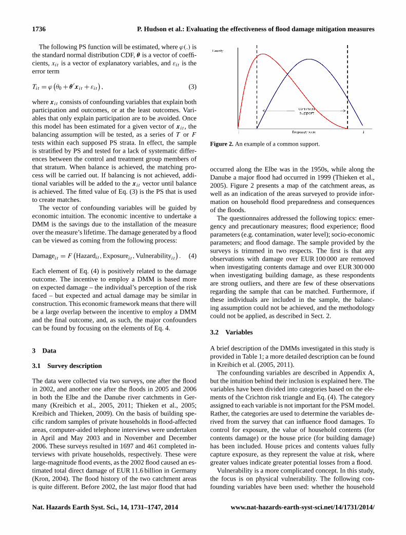
Condition 3:Overlap– the probability distributions forthe control and treatment group share a common sup-port, as in Fig. 1.

Condition 1 means that treatment participation and poten-tial outcomes are independent of one another, conditional onthe PS; in effect achievingy1 or y0 is as good as random. Therole of Condition 1 is that, by conditioning on the set of con-founders, the selection bias in the treatment is removed. Un-confoundedness holds when all the confounders have beenincluded in generating the PS.

Condition 2 is that, when conditioned onp(X), treatmentparticipation and individual traits are independent of one an-other. When Condition 2 holds, the PS is a balancing score,and then matching on the value of the PS achieves the sameas conditioning on each individual confounder value.

Condition 3 implies that the observations have a similar-enough PS to create a good match of individuals. Heckmanet al. (1996) provide a formulation of the bias introduced dueto matching, showing that the smaller the common support,

Figure 1. A map of the survey locations and river catchment areas.

the greater the possible bias in the final estimate (an exam-ple of a common support is displayed in Fig. 1). The reasonis that outside this range the matched participants are poten-tially too different from one another. Heckman et al. (1996)then proceed to state that by only matching over PS located inthe common support this matching quality bias is removed.Matching quality bias is introduced when matched individu-als are too different from each another.

Taken together Conditions 1 and 3 remove bias from theestimate, while Condition 2 allows for matching based on asingle value constructed from all the confounders.

In most cases, a probit or logit model will estimate thePS1. It has been found that using an estimate of the PS ratherthan the true PS (the actual probability for an individual toemploy a DMM) can increase efficiency (Rosenbaum, 1987;Robins et al., 1995; Rubin and Thomas, 1996; Heckmen etal., 1998; Hirano et al., 2003). The variables to be includedin the PS model need to meet the aims of Conditions 1 and 2.Brookhart et al. (2006) find that including variables that areonly connected to outcomes tends to reduce the variance ofthe final estimate, while variables that only affect participa-tion tend to increase the variance. Taken together, this impliesthat variables connected to outcomes should be included;their inclusion reduces bias or at least reduces the variance

1These are non-linear regression models; the advantage of thesemodels is that they will always predict a value for the dependentvariable that is bounded by 0 and 1. A probit model is described inEq. (3). A logit model uses a logistic distribution instead of a normaldistribution. The models report rescaled estimates of coefficients.



of the model2. However, there is a trade-off because the morevariables in the PS function, the smaller the potential overlapbetween the probability distributions.

The evaluation of the PS is not focused on the quality ofthe PS estimates, in the sense that the estimated PS is closeto the true PS, or that the regression used to estimate the PSis consistent (unbiased). The role of the PS is solely to col-lapse the relevant information into a single value, which isachieved upon balancing (Rosenbaum, 2002). Furthermore,the actual estimated coefficients of the probit or logit modelare also unimportant; evaluation is based solely on achiev-ing the conditions of balancing, unconfoundedness, and suf-ficient overlap.

Once Conditions 1–3 are deemed to hold, a matching al-gorithm must be selected. The algorithm will find for eachagent in the treatment group (a) member(s) of the controlgroup who has (have) a similar-enough PS, and these two arematched; the average difference between the outcomes (flooddamage) of the matches is an estimate of the ATT. There areseveral methods for the matching process:

1. Nearest-neighbour matching: a match is the person withthe closest PS to the observation of interest, but locatedin the control group. However, it may be that the near-est neighbour is very far away, in terms of the PS, in-creasing the potential bias of the estimate, due to poor-quality matches. With this method, matching with, orwithout, replacement can have a large effect. This is be-cause by matching without replacement, an individualis out of the sample once it has been matched. If thisindividual would have been a good match for anotheragent, then a worse match for that agent must be made.Matching with replacement solves this issue, and the or-dering of data will no longer be important, but the use ofless unique information can increase the variance. Thetrade-off to be made is between bias reduction (match-ing with replacement) and precision (matching withoutreplacement).

2. Caliper/radius matching: caliper matching creates amatch by accepting any PS as viable if it lies withina bandwidth around the PS in which we are interestedin for example±2 %. The benefit of this method is thatthe number of bad matches will be reduced due to thebandwidth. However it is possible that fewer matchesmay be made compared with nearest-neighbour match-ing, as, if no agent is located inside the caliper, thenthere is no match. Radius matching is an extension ofthis approach because it matches all the observations

2If the unconfoundedness assumption holds, each matching es-timate will tend towards the same value. However, if unconfound-edness does not hold, then adding variables that only influence out-comes will not mean that the different matching estimates will al-ways tend towards one another, as each matching method may becentred around a different expected value.

found inside the bandwidth. There is no strong reasonto select one bandwidth over another, a priori, as thereis a trade-off between the number of matches that canbe made against the bias of the matches.

3. Stratification matching: the area of PS overlap is par-titioned into intervals or strata. Each stratum is definedover a specific range of the PS, e.g. [0.1, 0.3], and withineach strata there are no statistically significant differ-ences between the traits of the treatment and those ofthe control groups. The overall ATT is estimated by firstsolving for the ATT within each strata, and then usinga weighted average of the strata ATT. These strata arecommonly the same as those used to test the balancingassumption.

4. Kernel matching: kernel models use a weighted averageof all of the observations in the control group to creatematches for the members of the treatment group, wherethe greater the distance between the PSs, the lower theweight. As such models use all the members of the con-trol group to create a counterfactual observation for atreatment group member, bad matches will be includedin the process. However, the weighting process reducesthe influence of bad matches, mitigating their influence.The bandwidth of the kernel is very important, as it de-termines the degree of smoothing, and large bandwidthsmay introduce bias into the estimated ATT. While thebandwidth is important, it is unclear what the correctbandwidth is before the investigation begins. Selectionof the bandwidth should be treated as a trade-off be-tween bias and variance.

Caliendo and Kopeinig (2005) state that there is no sin-gle preferred matching method, as the suitability of eachmatching method is dependent on the features of the dataconcerned, but, as the number of possible matches increases,the estimates of each matching method will tend towards thesame value. Nevertheless, in small samples, matching withreplacement is clearly preferred in order to maximise thenumber of possible matches. Additionally, if there are a largenumber of unmatched control group members, then a ker-nel matching method may be useful (Caliendo and Kopeinig,2005) to capture this otherwise lost information. The variousmeasures do allow for a robustness check of the estimated PS(and, as such, the estimated ATT), as, if Conditions 1 and 2hold, then they should provide an equally consistent estimateof the ATT. If there is a large difference between estimates,then a detailed investigation to find the missing confounderwill be required, so that the estimated PS can be made morereliable. As such, in small samples, a set of consistent re-sults may indicate that a suitable set of confounders has beenfound. All of the above matching methods are used here toact as a robustness test and to provide an average estimate ofthe bias due to selection bias.



The following PS function will be estimated, whereϕ(.) isthe standard normal distribution CDF,θ is a vector of coeffi-cients,xit is a vector of explanatory variables, andεit is theerror term

Tit = ϕ(θ0 + θ ′xit + εit

), (3)

wherexit consists of confounding variables that explain bothparticipation and outcomes, or at the least outcomes. Vari-ables that only explain participation are to be avoided. Oncethis model has been estimated for a given vector ofxit , thebalancing assumption will be tested, as a series ofT or F

tests within each supposed PS strata. In effect, the sampleis stratified by PS and tested for a lack of systematic differ-ences between the control and treatment group members ofthat stratum. When balance is achieved, the matching pro-cess will be carried out. If balancing is not achieved, addi-tional variables will be added to thexit vector until balanceis achieved. The fitted value of Eq. (3) is the PS that is usedto create matches.

The vector of confounding variables will be guided byeconomic intuition. The economic incentive to undertake aDMM is the savings due to the installation of the measureover the measure’s lifetime. The damage generated by a floodcan be viewed as coming from the following process:

Damageit = F(Hazardit ,Exposureit ,Vulnerabilityit

). (4)

Each element of Eq. (4) is positively related to the damageoutcome. The incentive to employ a DMM is based moreon expected damage – the individual’s perception of the riskfaced – but expected and actual damage may be similar inconstruction. This economic framework means that there willbe a large overlap between the incentive to employ a DMMand the final outcome, and, as such, the major confounderscan be found by focusing on the elements of Eq. 4.

3 Data

3.1 Survey description

The data were collected via two surveys, one after the floodin 2002, and another one after the floods in 2005 and 2006in both the Elbe and the Danube river catchments in Ger-many (Kreibich et al., 2005, 2011; Thieken et al., 2005;Kreibich and Thieken, 2009). On the basis of building spe-cific random samples of private households in flood-affectedareas, computer-aided telephone interviews were undertakenin April and May 2003 and in November and December2006. These surveys resulted in 1697 and 461 completed in-terviews with private households, respectively. These werelarge-magnitude flood events, as the 2002 flood caused an es-timated total direct damage of EUR 11.6 billion in Germany(Kron, 2004). The flood history of the two catchment areasis quite different. Before 2002, the last major flood that had

37

1 2

Figure 1. An example of a common support 3

4

5

6

7

8

9

10

11

12

13

14

15

16

17

18

19

Figure 2. An example of a common support.

occurred along the Elbe was in the 1950s, while along theDanube a major flood had occurred in 1999 (Thieken et al.,2005). Figure 2 presents a map of the catchment areas, aswell as an indication of the areas surveyed to provide infor-mation on household flood preparedness and consequencesof the floods.

The questionnaires addressed the following topics: emer-gency and precautionary measures; flood experience; floodparameters (e.g. contamination, water level); socio-economicparameters; and flood damage. The sample provided by thesurveys is trimmed in two respects. The first is that anyobservations with damage over EUR 100 000 are removedwhen investigating contents damage and over EUR 300 000when investigating building damage, as these respondentsare strong outliers, and there are few of these observationsregarding the sample that can be matched. Furthermore, ifthese individuals are included in the sample, the balanc-ing assumption could not be achieved, and the methodologycould not be applied, as described in Sect. 2.

3.2 Variables

A brief description of the DMMs investigated in this study isprovided in Table 1; a more detailed description can be foundin Kreibich et al. (2005, 2011).

The confounding variables are described in Appendix A,but the intuition behind their inclusion is explained here. Thevariables have been divided into categories based on the ele-ments of the Crichton risk triangle and Eq. (4). The categoryassigned to each variable is not important for the PSM model.Rather, the categories are used to determine the variables de-rived from the survey that can influence flood damages. Tocontrol for exposure, the value of household contents (forcontents damage) or the house price (for building damage)has been included. House prices and contents values fullycapture exposure, as they represent the value at risk, wheregreater values indicate greater potential losses from a flood.

Vulnerability is a more complicated concept. In this study,the focus is on physical vulnerability. The following con-founding variables have been used: whether the household



Table 1.Flood DMMs.

DMM Description

Flood- Use in a low-value way the floodadapted endangered floors, to keep possibleuse flood damage low, e.g. storing only

low-value items in flood-prone areas.

Flood- Avoid valuable, fixed units as interioradapted fitting in the flood-endangered floors,interior but use water-resistant or easily replaceablefitting materials for interior fitting.

Adapted Adapting the building structure, e.g. hadbuilding an especially stable building foundation,structure or waterproof sealed cellar walls.

Water Mobile barriers to prevent water enteringbarriers the building, e.g., sandbags or local small

flood protection walls.

has a cellar as these houses generally experience higher flooddamage (Kreibich et al., 2011), the age of the building, thequality of the building materials, and whether the buildingis located in an urban environment. Floor space is used toproxy the size of the building, as larger buildings may bemore likely to come into contact with floodwaters. Whererequired, either to reduce an ATT’s variance or to achievethe balancing assumption, the quality and duration of a floodwarning was also included. A warning provides time to makesure that static DMMs are used correctly or allows mobilemeasures, like “water barriers” for example, to be employed.

The following variables are used to control for the haz-ard that the respondents faced: flood water height insidethe building; flood duration; contamination of flood water;the return period of the flood; velocity; flood experience;whether the building could not be used while flooded; andwhether the building is located along the Elbe river (as com-pared to the Danube river).

It should be noted that above variables might not be use-able for all potential PS functions that analyse a DMM. Thisis because a variable should be reasonably unaffected by theuse of the particular DMM, and certain measures are aimedat directly altering these variables. This problem occurs withwater barriers, which potentially affect water height, flow ve-locity, and the duration that a building was flooded. In prin-ciple the same set of confounders is used to construct thePS for each DMM. However, when certain variables wereincluded it proved impossible to achieve the balancing as-sumption. Therefore, not every variable could be included ineach PS function. The list of variables included in each PSfunction is displayed in Table A1.

In order to retain as much information as possible and toachieve the balancing assumption, the survey variables werecoded in the following manner. Where a variable was cate-gorical, the categories were treated as separate binary vari-

ables, and a binary dummy variable was created for each cat-egory. Variables such as water height and duration were leftas continuous variables.

However, occasionally one of the categorical confound-ing variables was dropped from the PS function. Removinga categorical confounding variable will not completely re-move all of the information contained by this variable3, pos-sibly only altering the variance of the model. However, thereis a core set of variables included in each PS function basedon housing type and quality; whether the building has a cel-lar; total floor space; building/contents value; building age;experiences relating to the 2002 (or later) flood(s); warningduration; and how often the individual has been affected byflooding in the past. These variables as a whole capture theelements of Eq. (4) quite well. For example, contents valuewould capture the level of contents exposure completely. Themethodological approach followed was that the core vari-ables are included in every PS model, and additional vari-ables are added as required to achieve balance or to improvethe variance of the estimates.

Once the PS has been estimated, only observations withPSs within the common support are retained. The com-mon support is determined by removing any observa-tion that has a PS that lies outside the following range:[max

(PScontrol

min ,PStreatmentmin

),min

(PScontrol

max ,PStreatmentmax

)].

4 Estimation results

4.1 ATT estimates

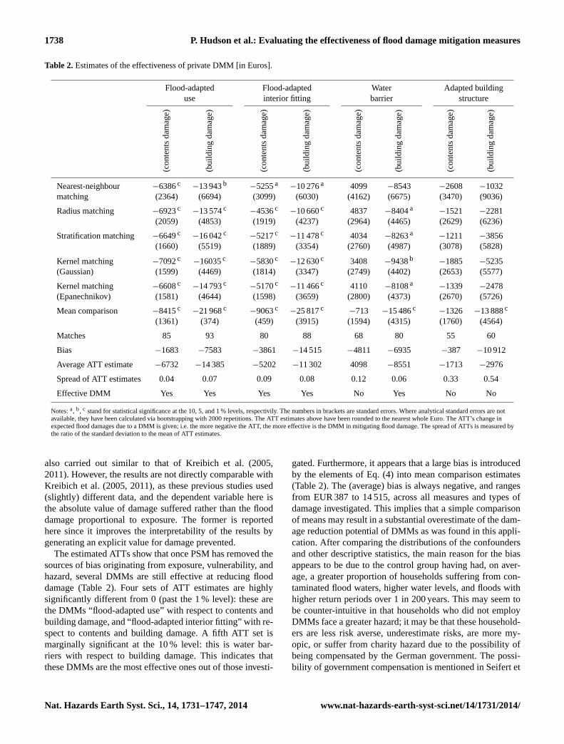
The ATT estimates are presented in Table 2 for the fivematching methods used. Several methods were used to testthe consistency of the ATT estimates, and infer the validityof the confounding variable vector. In particular, the ratio ofthe standard deviation to the mean of a set of ATT estimateswas calculated as a consistency indicator (Table 2). This in-dicator ranges in value from 0.04 to 0.54, where the smallerthe value, the smaller the spread of ATT estimates. Some ofthe DMMs have ATT estimates that are very strongly con-centrated around a central value. As an illustration, for thesignificantly effective DMMs (the effective measures, thoughwater barriers are only partial successful), the above consis-tency indicator ranges from 0.04 to 0.08. However, for theineffective measures the indicator ranges from 0.12 to 0.54.This indicator is especially large for “adapted building struc-ture”, namely 0.33–0.54, implying that a confounding vari-able may be missing from the PS function due to the greaterspread of estimated ATT values.

In order to have an overview of the potential bias ina DMM’s estimated effectiveness a mean comparison is

3When a categorical variable is converted into a series of dummyvariables, for mathematical reasons, at least one category must beskipped to form the base category, and any other category skippedwill also be a part of this base group.



Table 2.Estimates of the effectiveness of private DMM [in Euros].

Flood-adapted Flood-adapted Water Adapted buildinguse interior fitting barrier structure

(con

tent

sda

mag

e)

(bui

ldin

gda

mag

e)

(con

tent

sda

mag

e)

(bui

ldin

gda

mag

e)

(con

tent

sda

mag

e)

(bui

ldin

gda

mag

e)

(con

tent

sda

mag

e)

(bui

ldin

gda

mag

e)

Nearest-neighbour −6386c−13 943b

−5255a−10 276a 4099 −8543 −2608 −1032

matching (2364) (6694) (3099) (6030) (4162) (6675) (3470) (9036)

Radius matching −6923c−13 574c

−4536c−10 660c 4837 −8404a

−1521 −2281(2059) (4853) (1919) (4237) (2964) (4465) (2629) (6236)

Stratification matching −6649c−16 042c

−5217c−11 478c 4034 −8263a

−1211 −3856(1660) (5519) (1889) (3354) (2760) (4987) (3078) (5828)

Kernel matching −7092c−16035c

−5830c−12 630c 3408 −9438b

−1885 −5235(Gaussian) (1599) (4469) (1814) (3347) (2749) (4402) (2653) (5577)

Kernel matching −6608c−14 793c

−5170c−11 466c 4110 −8108a

−1339 −2478(Epanechnikov) (1581) (4644) (1598) (3659) (2800) (4373) (2670) (5726)

Mean comparison −8415c−21 968c

−9063c−25 817c

−713 −15 486c−1326 −13 888c

(1361) (374) (459) (3915) (1594) (4315) (1760) (4564)

Matches 85 93 80 88 68 80 55 60

Bias −1683 −7583 −3861 −14 515 −4811 −6935 −387 −10 912

Average ATT estimate −6732 −14 385 −5202 −11 302 4098 −8551 −1713 −2976

Spread of ATT estimates 0.04 0.07 0.09 0.08 0.12 0.06 0.33 0.54

Effective DMM Yes Yes Yes Yes No Yes No No

Notes:a, b, c stand for statistical significance at the 10, 5, and 1 % levels, respectivily. The numbers in brackets are standard errors. Where analytical standard errors are notavailable, they have been calculated via bootstrapping with 2000 repetitions. The ATT estimates above have been rounded to the nearest whole Euro. The ATT’s change inexpected flood damages due to a DMM is given; i.e. the more negative the ATT, the more effective is the DMM in mitigating flood damage. The spread of ATTs is measured bythe ratio of the standard deviation to the mean of ATT estimates.

also carried out similar to that of Kreibich et al. (2005,2011). However, the results are not directly comparable withKreibich et al. (2005, 2011), as these previous studies used(slightly) different data, and the dependent variable here isthe absolute value of damage suffered rather than the flooddamage proportional to exposure. The former is reportedhere since it improves the interpretability of the results bygenerating an explicit value for damage prevented.

The estimated ATTs show that once PSM has removed thesources of bias originating from exposure, vulnerability, andhazard, several DMMs are still effective at reducing flooddamage (Table 2). Four sets of ATT estimates are highlysignificantly different from 0 (past the 1 % level): these arethe DMMs “flood-adapted use” with respect to contents andbuilding damage, and “flood-adapted interior fitting” with re-spect to contents and building damage. A fifth ATT set ismarginally significant at the 10 % level: this is water bar-riers with respect to building damage. This indicates thatthese DMMs are the most effective ones out of those investi-

gated. Furthermore, it appears that a large bias is introducedby the elements of Eq. (4) into mean comparison estimates(Table 2). The (average) bias is always negative, and rangesfrom EUR 387 to 14 515, across all measures and types ofdamage investigated. This implies that a simple comparisonof means may result in a substantial overestimate of the dam-age reduction potential of DMMs as was found in this appli-cation. After comparing the distributions of the confoundersand other descriptive statistics, the main reason for the biasappears to be due to the control group having had, on aver-age, a greater proportion of households suffering from con-taminated flood waters, higher water levels, and floods withhigher return periods over 1 in 200 years. This may seem tobe counter-intuitive in that households who did not employDMMs face a greater hazard; it may be that these household-ers are less risk averse, underestimate risks, are more my-opic, or suffer from charity hazard due to the possibility ofbeing compensated by the German government. The possi-bility of government compensation is mentioned in Seifert et



al. (2013). It may also be simply an idiosyncratic feature ofthese flood events, and for a different series of flood eventsthe potential bias may be reversed. Exposure and vulnera-bility indicators seem rather similar across the two groups.While exposure and vulnerability indicators are required toremove bias in the estimated ATT, because they are impor-tant confounders at an individual level, the larger degree ofdifference in hazard seems to be the major source of biasin this application. The reason is that these distributions aremost divergent across the groups. Therefore, a simple meandifference in damage fails to account for the differing sever-ity of the floods affecting the control and treatment group.

The DMMs flood-adapted use and flood-adapted inte-rior fitting are still very effective when bias has been re-moved, as these measures have prevented, respectively, aboutEUR 6700 and 5200 of contents damage. The selection biaspresent in mean comparisons is rather substantial, as forflood-adapted use the bias is 25 % of the size of the estimatedATT, while, for flood-adapted interior fitting, the selectionbias is 74 % of the size of the ATT. Selection bias appears tobe a very powerful masking force in a mean comparison.

It appears that flood-adapted use (e.g. storing only low-value items in flood-prone storeys) is more effective thanflood-adapted interior fitting (e.g. using flood-resistant mate-rials to construct interior fittings) for reducing contents dam-age, which is most likely because the former is a direct mea-sure for limiting the impacts of floods on contents, whileflood-adapted interior fitting would be an indirect way ofreducing contents damage due to storage units being moreflood safe. The two measures work by altering different as-pects of Eq. (4); flood-adapted use alters the effective level ofexposure, while flood-adapted interior fitting would reducethe vulnerability of household storage units.

The measures that are effective at reducing building dam-age – i.e. flood-adapted use, flood-adapted interior fitting,and water barriers – again suffer from a substantial bias ofEUR 7583, 14515, and 6935, respectively. As a percentageof the ATT, this bias is 55, 128, and 81 %. The bias regard-ing building damage as a proportion of the ATT is, on thewhole, larger than that present in the estimated ATTs relatingto content damage. Flood-adapted use, flood-adapted interiorfitting, and water barrier are still potentially very effectiveDMMs, preventing EUR 14 385, 11 302 or 8551 of buildingdamages, respectively. Flood-adapted interior fitting is moreeffective than water barriers at reducing building damage be-cause it has reduced the vulnerability level of the building.Water barriers would reduce the amount of water enteringthe house, but, dependent on the magnitude of the flood, maybe overtopped and then would not work at all. Consideringthe magnitude of the floods suffered, which was up to a 1 in500-year return period in some cases (Risk Management So-lutions, 2003), it may be that water barriers may be more ef-fective at reducing building damages incurred from smaller-magnitude flood events. The series of strategies represented

by flood-adapted use would have caused its reduction in dam-ages due to lower levels of exposure in floodable areas.

Adapted building structure was, via a mean comparison,detected to have no significant effect of reducing contentsdamage, and, even controlling for bias via PSM, it is stillineffective. A further finding is that, if nearest-neighbourmatching is ignored, then the average bias is only aboutEUR 150. Such a remarkably close estimate in a small sam-ple could mean that, for this measure, its implementationcould be almost as good as random. If all estimated ATTs areincluded, then the bias increases to 16 % of the average ATTfor this DMM. This observation reinforces the misleadingnature of mean comparisons because sometimes a mean com-parison is an accurate estimation technique, while in othercases it is not. The results for adapted building structureregarding building damage are the most inconsistent set ofATT estimates. This may indicate that there is a missing con-founder in the relationship between adapted building struc-ture and building damage, as, if the whole set of confounderswas found, then the estimated ATTs should be closer togetherin value. This inconsistency means that any inference aboutadapted building structure and building damage (and to asmaller degree contents damage) should be treated with cau-tion.

The measure that seems most effective is flood-adapteduse as it has a substantial impact on both building and con-tents damages, being closely followed by food-adapted inte-rior fitting. Flood-adapted interior fitting may be less effec-tive because damage in this paper is measured via replace-ment values; flood-adapted use aims at reducing this valuewhile flood-adapted interior fitting does not. An interestingobservation from the ATT estimates is that water barriers hada very different effect on contents and building damage. Thesame measure had a positive (insignificant) ATT regardingcontents damage and a negative ATT for building damage,from which it can be inferred that water barriers were ef-fective at protecting the building but not its contents. Thiscould be an artefact of an incomplete set of confounders,but this argument fails to explain why water barriers protectthe building. Compared with the other measures that protecthousehold contents the use of water barriers may have re-duced an individual’s efforts to take other measures that limitflood damage.

4.2 Sensitivity analysis

Table 3 presents the results of a sensitivity analysis using themethodology suggested in Rosenbaum (2002), who attemptsto provide an indication of the possible strength that an ex-cluded confounder would require to alter the results quali-tatively. It must be kept in mind that the results of this in-vestigation cannot be viewed as a test of the unconfounded-ness assumption. The two areas of sensitivity presented arethe bounds on possible statistical significance and the poten-tial 95 % confidence interval around the ATT estimate. The



Table 3.Sensitivity analysis.

Measure Matching method Statistical 95 % confidence intervalsignificance of the ATT includes 0

Flood-adapted use (contents damage) Nearest neighbour 1.4 1.2Kernel matching (Gaussian) 3.4 2.8Kernel matching (Epanechnikov) 3.2 2.6Radius matching 3.3 2.6

Flood-adapted use (building damage) Nearest neighbour 1.2 1.1Kernel matching (Gaussian) 2.5 2.1Kernel matching (Epanechnikov) 2.4 2.0Radius matching 1.6 1.3

Flood-adapted interior fitting (contents damage) Nearest neighbour 1.7 1.4Kernel matching (Gaussian) 2.5 2.1Kernel matching (Epanechnikov) 2.3 1.9Radius matching 2.2 1.8

Flood-adapted interior fitting (building damage) Nearest neighbour 1.4 1.2Kernel matching (Gaussian) 3.4 2.7Kernel matching (Epanechnikov) 3.2 2.6Radius matching 3 2.5

Water barriers (building damage) Kernel matching (Gaussian) 1.5 1.2Kernel matching (Epanechnikov) 1.4 1.2Radius matching 1.4 1.2

Notes: the sensitivity to excluded confounders can be estimated for each matching method used, but to save on space only three matching methods have been selected.For statistical significance the number presented refers to the gamma required to reduce significance to past the 10 % level.

way to understand the sensitivity results is as follows: for ex-ample, suppose0 = 3; then an excluded confounder wouldhave to change the participation odds by threefold for theobserved result to become statistically insignificant at theselected level. This would indicate an ATT estimate that isvery insensitive to possibly excluded confounders, and thatinference based on the estimated ATT is more reliable thanfor lower values of0. Sensitivity to potential excluded con-founders, in this study, will be judged upon what strengthof confounder would be required to remove statistical sig-nificance at the 10 % level. In addition, it is examined whatwould be required for the possible 95 % confidence intervalof estimates to include 0. The 95 % confidence interval al-ways contains 0 for the results found to be statistically in-significant, i.e. water barriers with respect to contents dam-age and adapted building structure with respect to contentsand building damage. Thus, Table 3 only presents the resultsof this sensitivity analysis for the DMMs that were found tohave a statistically significant effect (up to and including the10 % level).

On the whole flood-adapted use (contents damage) andflood-adapted interior fitting (contents and building damage)ATT estimates are fairly robust to the possible presence ofa missing confounder since, except for nearest-neighbourmatching, to remove the statistical significance of the resultswould require a possible confounder to alter the odds ratioby over 200 %. As all relevant and applicable variables from

the original survey were included, it is not likely to be thecase that such a powerful confounder would have been ex-cluded. The water barriers measure on the other hand is lessrobust as a possibly excluded confounder would have to alterthe odds ratio by only 20 % to significantly change results.It must be kept in mind that when the ATT for water barri-ers was estimated, because of survey design, it was not ableto have a large range of confounders for the hazard compo-nent of risk. A large number of hazard variables would bedirectly affected by the measure, and the use of these partic-ular variables would confuse the causal direction of the esti-mates. It is likely that the negative effect on building damageis still an overestimate, judging from the previously foundimportance of hazard characteristics. As the complete rangeof hazard variables seems to be a major source of bias, it islikely that if the complete range of hazard variables couldbe included in the confounding vector for water barriers itwould alter participation odds by more than 20 %. There-fore, although water barriers seem to reduce building dam-age, this result should be treated with caution. Flood-adapteduse appears to be more sensitive to missing confounders re-garding building damage compared with contents damage.It is difficult to judge how robust this measure is comparedwith water barriers. For kernel matching, flood-adapted use(building damages) seems to be fairly sensitive and more sothan water barriers, while for nearest-neighbour and radiusmatching the results are less sensitive than those for water



barriers. However, compared to water barriers, flood-adapteduse (building damages) contains a more complete range ofvariables (mainly regarding the hazard), making it less likelythat a confounder has been excluded from the model. The re-sults of table three may indicate that certain DMMs are quitesensitive to missing confounders. However, this finding mustbe balanced against the smaller likelihood that relevant con-founders are actually missing from the model.

5 Discussion

5.1 Discussion of DMM effectiveness

The application of PSM to flood damage survey data is ableto remove the substantial bias present in estimates of dam-age reduction via DMMs based on simple mean compar-isons. The bias removed is large, as for the statistically signif-icant content-related measures the bias is around EUR 1700–3900, while for building-damage-related measures the biasis around EUR 6900–14 500. In all cases, the biases are asubstantial proportion of the ATT. PSM allows us to providea more accurate estimate of a DMM’s effectiveness, whilemaintaining as wide a sample as possible. The ATT estimatesdisplayed in the previous section are a refinement of previ-ous estimates of DMMs in Germany (Kreibich et al., 2005,2011).

Once bias-corrected estimates have been produced the ef-fectiveness of private DMMs was found to be less than pre-viously estimated by a comparison of mean damage. Nev-ertheless, the overall picture of effective DMMs has not al-tered substantially as only one previously detected effectivemeasure – namely adapted building structure in respect tobuilding damage (Kreibich et al., 2005) – has been reducedto marginal effectiveness. The most effective DMM is flood-adapted use, followed by flood-adapted interior fitting. Thisis due to their ability to significantly reduce both contentsand building damages. Flood-adapted use may also be morefavourable, because as a series of coping strategies it mayinvolve smaller installation costs than other measures. Thereasons for the effectiveness of the various measures are de-scribed in detail in Kreibich et al. (2005, 2011). Kreibich etal. (2011) also provides indications of the costs of installingvarious DMMs, estimated for a model building, i.e. for adetached, solid single-family house with a property area of750 m2, from which the cost–benefit ratios of some of thecurrently investigated DMMs can be calculated. The success-ful measure common to this study and Kreibich et al. (2011)is water barriers. Kreibich et al. (2011) provide a cost es-timate of EUR 6100 for installing 10 m of water barriers.Assuming that a flood affects a building every year, the ex-pected lifetime discounted (discounted at 3 %) cost–benefitratio is 22.3. The less often a flood is expected to occur, thesmaller the cost–benefit ratio, until the break-even point isreached with an expected flood frequency of around once ev-ery 22 years.

The first implication for future flood risk managementis that flood-adapted use and flood-adapted interior fittingshould be expanded due to their double dividend return foronly one set of installation costs. The next implication isthat, while individual level DMMs measures do still seemto be powerful tools for limiting flood risk, the role of DMM,as part of current risk management strategies, should be al-tered to take into account the finding that they are less effec-tive than previously believed. This reduction in effectivenessconfirms the importance of multiple stakeholders undertak-ing action as a part of a risk management strategy. A relatedimplication is that, as selection bias was a prominent fea-ture of this study, the possible presence of selection bias inevaluations of non-randomly employed flood risk manage-ment strategies (e.g. the success of a flood warning system)is a concern. Therefore, evaluation techniques that control formany sources of bias simultaneously are required to produceaccurate evaluations to guide more productive risk manage-ment policies.

It should be noted that the above policy implications arebased on the experience of three floods with high overall re-turn periods and water depths. For instance, the average wa-ter depth for the treatment group (averaged over all DMMs)it is approximately 30 cm, while for the control group (aver-aged over all DMMs) is approximately 80 cm. The largestgap is for Flood adapted interior fitting at nearly 70 cm.The investigated DMMs might respond differently if aver-age floodwater heights were systematically lower across thesample population. While PSM controlled for many sourcesof bias, it would be useful to analyse in more detail how wellthe investigated measures perform under a wider range offlood events and in different regions. For instance water bar-riers may be more effective in limiting the damage of morefrequent flood events with shallow water depths. Conductingan investigation of the effectiveness of DMMs that covers awider range of flood events and geographical areas, while us-ing PSM, could create a more readily generalisable result andpolicy implications.

5.2 Discussion of the application of PSM

The value added of PSM in the current application is depen-dent on the inferred size of selection bias. The estimates ofselection bias contained in mean comparison estimates rangefrom 16 to 128 % of the size of the ATT. Therefore, selectionbias can create quite misleading inferences about the ATTas in one case (water barriers for building damages) the biasis larger than the ATT estimate. The wide range of selec-tion bias indicates a strong possibility for misleading infer-ences to be made from simple evaluation techniques. There-fore, evaluation techniques that provide a way of controllingfor the possibility of large selection bias effects are required.PSM is a technique that is able to achieve the possible re-moval of selection bias.



The applicability of PSM is strengthened by the abilityto employ many different ways of creating a match. Thisis because the more consistent the results of several match-ing methods are, the more likely it is that unconfounded-ness holds. This becomes apparent from the results of differ-ent matching methods for flood-adapted use (contents dam-age) and adapted building structure (building damage). Theestimates for flood-adapted use are very closely scatteredtogether. However, the ATT estimates for adapted buildingstructure (building damage) is about 13 times as wide as thatof flood-adapted use. Additionally, by using several match-ing methods, patterns in the ATT estimates can be revealed.These patterns can allow inference about the true value of theATT in a way that a single estimate may not. For example,adapted building structure (contents damage) provides fourestimates that seem to be centred around a value of−1500,while the fifth is −2600. This could indicate that the truevalue is more closely centred on−1500.

It appears that direct measures of exposure performed bet-ter than indirect measures; e.g. contents value is preferredto income. Furthermore, it appears that differences in haz-ard were a major source of bias. Therefore, a wide range ofquestions relating to hazard characteristics should be asked.This study successfully applied the following core variablesto each PS function: contents or building value; flood expe-rience; flood water depth and duration; water contamination;flow velocity; building age; and housing material quality. Arelated recommendation is that the survey must contain notonly all of the relevant confounders, but additionally vari-ables that explain outcomes. Relevant confounders can bedifficult to identify, as they require a synthesis of the liter-ature that investigates flood damage outcomes and the useof DMMs. The survey questions should also be presented ina way that allows for the easy construction of dummy vari-ables based on variables that only explain damage outcomes.These variables would provide ample scope for meeting thebalancing assumption and reducing the models’ variance.

The application of PSM also indicated that large samplesare very useful. Large samples are useful as it is possiblethat in a flood-affected area the treatment group could be rel-atively small, simply because few people in the area havechosen to employ a particular DMM. Sampling highly flood-prone areas may also solve this issue, as there is a strongerincentive in these areas to employ a DMM. However, thispotentially makes the sample less representative of the largerpopulation at risk. While it is difficult to judge the small-est number of matches that produces a reliable estimate ofthe ATT, Prirracchio et al. (2012) note that using nearest-neighbour matching (without replacement) and a sample size(total participants) of 40 resulted in a maximum relative biasof 10 %4. From Prirracchio et al. (2012), it can be inferred

4The estimated ATT compared with the true ATT; in Priracchioet al. (2012) they are able to calculate this comparison as they fixthe value of the true ATT in their simulations. Furthermore, recall

that a sample of 100 has a relative bias of 3 %, while witha sample of 600 (the total sample in our application was ap-proximately 640) it is approximately 1.5 %. It is difficult togeneralise this, but, when combined with the arguments ofHolmes and Olsen (2010) and Caliendo and Kopeinig (2005),if several matching methods produce similar results, even insmall samples, then these results appear to be robust.

The application of PSM seemed to indicate that the rela-tionship between different DMMs and the confounders maybe different between measures. For instance, receiving aflood warning can be a confounder for the use of mobile floodbarriers, but not for static DMMs. Moreover, a variable mayallow for balancing in one equation, while in another its pres-ence may invalidate this assumption. Both of these problemsmean that an inflexible approach to selecting PS variables isto be avoided in order to increase the number of situationswhere PSM can be applied. The principal concern, however,should always be the strength of the unconfoundedness as-sumption.

6 Conclusions

The literature that evaluates DMMs using survey data islimited. Simple evaluation methodologies and small sam-ple numbers of observational data have the potential to cre-ate misleading inferences regarding the success of variousDMMs. This is due to confounding variables, which are vari-ables that explain both the outcomes and the use of a DMM,thereby introducing bias into the estimated effectiveness. Thecurrent study sought to remove confounding bias by apply-ing propensity score matching (PSM) to a sample of Ger-man households living along the Elbe and Danube rivers whowere surveyed in response to floods occurring in 2002, 2005,and 2006. PSM was applied in order to meet the first ob-jective of this study of more precisely evaluating the effec-tiveness of various DMMs. PSM removes confounding biasby matching every individual who uses a DMM with a suf-ficiently similar individual who did not employ the DMM inorder to form the required counterfactual observation. OncePSM had been applied, it was found that previous researchusing mean comparisons of flood damage could result in veryinaccurate estimates of the effectiveness of a DMM, due tothe presence of confounding variables. However, once PSMhas refined previous evaluation estimates by removing thelarge selection bias, it is found that several DMMs are stillvery effective measures for reducing flood risk at an individ-ual level. Moreover, the overall image of successful DMMsis broadly the same as revealed under previously used meth-ods, only their damage reducing effect is less than may havebeen previously inferred.

that all estimated values would display a bias that will tend towards0 as the sample size increases, conditional on unconfoundedness.



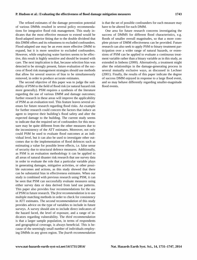
The refined estimates of the damage prevention potentialof various DMMs resulted in several policy recommenda-tions for integrative flood risk management. This study in-dicates that the most effective measure to extend would beflood-adapted interior fitting due to the double dividend thatthis DMM offers and its robustness to excluded confounders.Flood-adapted use may be an even more effective DMM toexpand, but it is more sensitive to excluded confounders.However, while employing water barriers seems to be effec-tive, this result is highly sensitive and should be treated withcare. The next implication is that, because selection bias wasdetected to be strongly present, future evaluation of the suc-cess of flood risk management strategies should use methodsthat allow for several sources of bias to be simultaneouslyremoved, in order to produce accurate estimates.

The second objective of this paper was to judge the suit-ability of PSM to the field of flood risk (or natural hazard riskmore generally). PSM requires a synthesis of the literatureregarding the use of various DMM and damage outcomes;further research in these areas will improve the applicabilityof PSM as an evaluation tool. This feature leaves several av-enues for future research regarding flood risks. An examplefor further research could concern the factors that induce anagent to improve their building’s flood safety and alter theexpected damage to the building. The current study seemsto indicate that the required set of confounders for this mea-sure may be quite different from the other measures due tothe inconsistency of the ATT estimates. Moreover, not onlycould PSM be used to evaluate flood outcomes at an indi-vidual level, but it can also be used to investigate other out-comes due to the implementation of flood defences such asestimating a value for possible levee effects, i.e. false senseof security due to structural defence measures. Additionally,as PSM is an evaluation methodology it can be applied toall areas of natural disaster risk research that use survey datain order to evaluate the role that a particular variable playsin generating damages, mitigative activities, or other possi-ble outcomes and actions, as this study showed that therecan be substantial bias in effectiveness estimates. When ourstudy is combined with previous research using PSM, it canbe seen that PSM can successfully evaluate measures usingeither survey data or data derived from land use patterns.This paper also provides four recommendations for the useof PSM in future research. Thefirst recommendationis to usemultiple matching methods in order to check for consistencyin ATT estimates. Thesecond recommendationof this studyprovides advice on the type of variables to include in futuresurveys. A survey should aim to include direct indicators ofthe hazard faced, the level of exposure, and a range of in-dicators regarding vulnerability. Thethird recommendationis that a larger sample population, in terms of respondentsand geographical coverage, is always beneficial. This is be-cause of the seemingly small number of individuals employ-ing DMMs in any given region. Thefourth recommendation

is that the set of possible confounders for each measure mayhave to be altered for each DMM.

One area for future research concerns investigating thesuccess of DMMS for different flood characteristics, e.g.floods of smaller overall magnitudes, so that a more com-plete picture of DMM effectiveness can be provided. Futureresearch can also seek to apply PSM to binary treatment par-ticipation over a wider range of natural hazards, or exten-sions of PSM can be applied to evaluate a continuous treat-ment variable rather than a binary variable as in this study, asextended in Imbens (2000). Alternatively, a treatment mightalter the relationships in the damage-generating process inseveral mutually exclusive ways, as discussed in Lechner(2001). Finally, the results of this paper indicate the degreeof success DMM enjoyed in response to a large flood event,and so may behave differently regarding smaller-magnitudeflood events.



Appendix A: Variable number, name, and description.

ATT = E(y1 − y0|T = 1) = E(y1|T = 1) − E(y0|T = 1)

The variables in italics below have been included in everyPS function, and are otherwise referred to as the core vari-ables. The variables presented in standard type are includedin models where they improved performance while maintain-ing the balancing assumption. Table A1 below lists the vari-ables included in each PS model. The possible variables tobe included in the PS function are as follows:

1. Household contents damage: damage to household con-tents, where contents are all moveable items in thehome. Measured in Euros, and as replacement costs.

2. Household building damage: damage to the building –repair costs. Measured in Euros.

3. Household contents value: the value of all moveableitems within the home.Measured in Euros.

4. Flood duration: the length of time the building wasflooded in hours.Measured in hours.

5. Flow speed 1: low water speed (stationary water is thebase group). From a 0–4 scale based on the scale de-veloped by the Bureau of Reclamation (Thieken et al.,2005). This is a dummy variable taking the value of 1 ifthe respondent provided a value of 1, and 0 otherwise.

6. Flow speed 2: medium water speed (stationary water isthe base group). From a 0–4 scale based on the scale de-veloped by the Bureau of Reclamation (Thieken, 2005).This is a dummy variable taking the value of 1 if therespondent provided a value of 1, and 0 otherwise.

7. Elbe: a dummy variable taking the value of 1 if the re-spondent lived along the Elbe river, and 0 otherwise.

8. Urban area: a dummy variable taking the value of 1if the respondent lived in an urban area (greater than50 000 residents), and 0 otherwise.

9. House age (1948): a dummy variable taking the value of1 if the respondent’s building was constructed between1948 and 1964, and 0 otherwise.



12. House age (2000): a dummy variable taking the valueof 1 if the respondent’s building was constructed after2000, and 0 otherwise.

13. House quality 2: a dummy variable taking the value of1 if the respondent said that the quality of their buildingwas 2 on a 6-point scale (1 is highest quality).

14. House quality 3: a dummy variable taking the value of1 if the respondent said that the quality of their buildingwas 3 on a 6-point scale (1 is highest quality).

15. House quality 3 plus: a dummy variable taking the valueof 1 if the respondent said that the quality of their build-ing was 4, 5, or 6 on a 6-point scale (1 is highest qual-ity).

16. Flood risk 1: a dummy variable taking the value of 1 ifthe respondent said that a flood had only affected themonce before.

17. Flood risk 2: a dummy variable taking the value of 1 ifthe respondent said that they have suffered twice fromflooding before.

18. Flood risk 3: a dummy variable taking the value of 1 ifthe respondent said that they have suffered three floodevents before.

19. Flood risk 4: a dummy variable taking the value of 1 ifthe respondent said that they have suffered from 4 floodevents before.

20. Flood risk 5: a dummy variable taking the value of 1 ifthe respondent said that they have suffered from morethan 5 floods before.

21. Water height: the height of floodwaters entering thehouse in metres.

22. Contaminated water: a dummy variable taking thevalue of 1 if the respondent’s house was contaminatedby sewage or oil, and 0 otherwise.

23. Warning duration: the length of time before a flood thata warning was issued in hours.

24. Return 1: a dummy variable taking the value of 1 if theflood recorded at the nearest gauge was between 1 in10yearsand 1 in 50years, and 0 otherwise.

25. Return 2: a dummy variable taking the value of 1 if theflood recorded at the nearest gauge was between 1 in50yearsand 1 in 200years, and 0 otherwise.

26. Return 3: a dummy variable taking the value of 1 ifthe flood recorded at the nearest gauge was over 1 in200years, and 0 otherwise.

27. Cellar: a dummy variable taking the value of 1 if thebuilding has a cellar, and 0 otherwise.

28. Floor size: the total floor space of the home, includingthe size of the cellar if present. Measured in m2.



29. House price: an estimate of the house price based onthe M1914 criteria. Measured in Euros.

30. Warning quality: a dummy taking on the value of 1 if theperceived quality of the flood warning is given a valueof 1, 2, or 3 on a scale of 0–11, and 0 otherwise.

31. Warning quality 2: a dummy taking on the value of 1if the perceived quality of the flood warning is given avalue of 4, 5, or 6 on a scale of 0–11, and 0 otherwise.

32. Warning quality : a dummy taking on the value of 1if the perceived quality of the flood warning is given avalue larger than 7 on a scale of 0–11, and 0 otherwise.

33. Renter: a dummy variable taking the value of 1 if theresident rents their residence, and 0 if they own theirplace of residence.

34. Detached house: a dummy variable taking the value 1(0 otherwise) if the building is a detached house (thisvariable is the core base category for housing type).

35. Semi-detached house: a dummy variable taking thevalue 1 (0 otherwise) if the building is a semi-detachedhouse.

36. Town house: a dummy variable taking the value 1 (0otherwise) if the building is a detached house.

37. Multi-family house: a dummy variable taking the value1 (0 otherwise) if the building is a multi-family house.

38. Commercial building: a dummy variable taking thevalue 1 (0 otherwise) if the building is a commercialbuilding.

39. Secured documents: a dummy variable taking the value1 (0 otherwise) if the responded secured their docu-ments before the flood.

40. Move cars: a dummy variable taking the value 1 (0 oth-erwise) if the respondent moved their car to a flood-safearea before the flood.

41. Move animals: a dummy variable taking the value 1 (0otherwise) if the respondent moved animals to a flood-safe location.

42. Turn off gas/electric: a dummy variable taking the value1 (0 otherwise) if the respondent turned off the mainselectric and gas.

43. Evacuation: a dummy variable taking the value 1 (0 oth-erwise) if the respondent had to vacate their buildingdue to the flood.

Table A1. Included confounders.

Flood-adapted use(contents damage) 3–28, 35–37, 39–40, 43

Flood-adapted use(building damage) 3–29, 33, 35, 36, 38, 43

Flood-adapted interior fitting(contents damage) 3–28, 35, 36, 38–41, 43

Flood-adapted interior fitting(building damage) 3–15, 17–32, 35, 36, 38, 43

Adapted building structure(contents damage) 3–8, 11–28, 35–37, 39–43

Adapted building structure(building damage) 3–8, 10–28, 30–32, 35–43

mobile water barrier(contents damage) 3–8, 10–28, 30–32, 35–43

mobile water barrier(building damage) 4–8, 10–27, 29–33, 35–37, 39

Notes: the confounders are referred to by their identifying numbers, which are listedabove.



Acknowledgements.The research leading to these results hasreceived funding from the EU 7th Framework Programme throughthe project ENHANCE (grant agreement no. 308438). The surveycollecting flood damage data of the 2005 and 2006 floods wasundertaken as part of the MEDIS project (Methods for the Evalu-ation of Direct and Indirect Flood Losses), funded by the GermanMinistry of Education and Research (BMBF) (no. 0330688). Thesurvey after the 2002 flood was undertaken under the auspicesof the German Research Network Natural Disasters (DFNK)and was funded by Deutsche Rückversicherung AG and BMBF(no. 01SFR9969/5). We would also like to thank the two anony-mous reviewers for their comments on improving the paper.

Edited by: H. de MoelReviewed by: two anonymous referees

References

Angrist, J. and Piske, J.: Mostly Harmless Econometrics, PrincetonUniversity Press, UK, 2009.

Bouwer, L., Bubeck, P., and Aerts, J.: Changes in future flood riskdue to climate and development in a Dutch polder area, Gover-nance, Complexity and Resilience, 20, 464–471, 2010.

Brookhart, M., Scheeweiss, S., Rothman, K., Glynn, R., Avorn, J.,and Strumer, T.: Variable section for Propensity Score Models,Am. J. Epidemiol., 163, 1149–1156, 2006.

Bubeck, P., Botzen, W. J. W., Kreibich, H., and Aerts, J. C. J. H.:Long-term development and effectiveness of private flood mit-igation measures: an analysis for the German part of theriver Rhine, Nat. Hazards Earth Syst. Sci., 12, 3507–3518,doi:10.5194/nhess-12-3507-2012, 2012.

Butry, D.: Fighting fire with fire: estimating the efficacy of wild-fire mitigation programs using propensity scores, Environ. Ecol.Stat., 16, 291–319, 2009.

Caliendo, M. and Kopeinig, S.: Some Practical Guidance for the Im-plementation of Propensity Score Matching, IZA DP No. 1588,2005.

Changnon, S., Pielke, R., Changnon, D., Sylves, R., and Pulwarty,R.: Human factors explain the increased losses from weather andclimate extremes, B. Am. Meteorol. Soc., 81, 437–442, 2000.

Crichton, D.: The risk triangle, in: Natural Disaster Management,edited by: Ingleton, J., Tudor Rose, London, 102–103, 1999.

D’Agostino, R.: Tutorial in biostatistics, propensity score methodsfor bias reduction in the comparison of a treatment to a non-randomized control group, Stat. Med., 17, 2265–2281, 1998.

DEFRA: Developing the evidence base for flood resistance and re-silience: summary report, R&TD technical report FD 2507/TRI,Environment Agency and the Department for the EnvironmentFood and Rural affairs (DEFRA), London, 2008.

Dehejia, R. and Wahba, S.: Propensity score-matching Methods fornon-experimental causal studies, Rev. Econ. Statistics, 84, 151–161, 2002.

De Moel, H., van Vliet, M., and Aerts, J.: Evaluating the effectof flood damage-reducing measures: a case study of the un-embanked area of Rotterdam, the Netherlands, Reg. Environ.Change, 14, 895–908, doi:10.1007/s10113-013-0420-z, 2014.

Dutta, D., Herath, S., and Musiakec, K.: A mathematical model forflood loss estimation, J. Hydrol., 277, 24–49, 2003.

Grossman, J. and Mackenzie, F.: The randomized controlled trial:gold standard, or merely standard, Perspect. Biol. Med., 48, 516–534, 2005.

Hall, J., Sayers, P., and Dawson, R.: National-scale assessment ofcurrent and future flood risk in England and Wales, Nat. Hazards,36, 147–164, 2005.

Heckman, J., Ichimura, H., Smith, J., and Todd, P.: Sources of selec-tion bias in evaluating social programs: An interpretation of con-ventional measures and evidence on the effectiveness of match-ing as a program evaluation method, P. Natl. Acad. Sci. USA, 93,12416–13420, 1996.

Hirano, K., Imbens, G., and Ridder, G.: Efficient estimation of aver-age treatment effects using estimated propensity scores, Econo-metrica, 71, 1161–1189, 2003.

Holmes, W. and Olsen, C.: Using propensity scores in small sam-ples, working paper, available at:http://www.faculty.umb.edu/william_holmes/usingpropensityscoreswithsmallsamples.pdf,last access: 23 December 2013, 2010.

Holub, M. and Fuchs, S.: Benefits of local structural protectionto mitigate torrent-related hazards, in: Risk Analysis VI, WIT,Transactions on Information and Communication Technologies,edited by: Brebbia, C. and Beriatos, E., WIT, Southampton, 39,401–411, 2008.

Imbens, G.: The role of the propensity score in estimating dose-response functions, Biometrika, 87, 706–710, 2000.

IPCC (Intergovernmental Panel on Climate Change): Managingthe Risks of Extreme Events and Disasters to Advance ClimateChange Adaptation, Cambridge University Press, New York,2012.

Kreibich, H. and Thieken, A.: Coping with floods in the city ofDresden, Germany, Nat. Hazards, 51, 423–436, 2009.

Kreibich, H., Thieken, A. H., Petrow, Th., Müller, M., and Merz,B.: Flood loss reduction of private households due to buildingprecautionary measures – lessons learned from the Elbe floodin August 2002, Nat. Hazards Earth Syst. Sci., 5, 117–126,doi:10.5194/nhess-5-117-2005, 2005.

Kreibich, H., Müller, M., Thieken, A. H., and Merz, B.: Flood pre-caution of companies and their ability to cope with the floodin August 2002 in Saxony, Germany, Water Resour. Res., 43,W03408, doi:10.1029/2005WR004691, 2007.

Kreibich, H., Christenberger, S., and Schwarze, R.: Economic mo-tivation of households to undertake private precautionary mea-sures against floods, Nat. Hazards Earth Syst. Sci., 11, 309–321,doi:10.5194/nhess-11-309-2011, 2011.

Kron, W.: Zunehmende Überschwemmungsschäden: eine Gefahrfür die Versicherungswirtschaft?, in: ATV-DVWK: Bundesta-gung, Würzburg, 15–16 September 2004, DCM, Meckenheim,47–63, 2004 (in German).

Kron, W.: Flood Risk, Hazard, Values, Vulnerability, Water Int., 30,58–68, doi:10.1080/02508060508691837, 2005.

Lechner, M: Identification and estimation of causal effects of multi-ple treatments under the conditional dependence assumption, in:Econometric Evaluation of Labour market Policies, edited by:Lechner, M. and Pfeiffer, F., ZEW Economic Studies, 13, 43–58,2001.

Milly, R., Wetherald, R., Dunne, K., and Delworth, T.: Increasingrisk of great floods in a changing climate, Nature, 415, 514–517,2002.


http://dx.doi.org/10.5194/nhess-12-3507-2012

http://dx.doi.org/10.1007/s10113-013-0420-z

http://www.faculty.umb.edu/william_ holmes/usingpropensityscoreswithsmallsamples.pdf

http://www.faculty.umb.edu/william_ holmes/usingpropensityscoreswithsmallsamples.pdf


http://dx.doi.org/10.1029/2005WR004691


http://dx.doi.org/10.1080/02508060508691837


Pirracchio, R., Resche-Rigon, M., and Chevret, S.: Evaluation ofthe propensity score methods for estimating marginal odds ra-tios in case of small sample, BMC Med. Res. Methodol., 12, 70,doi:10.1186/1471-2288-12-70, 2012.

Poussin, J. K., Bubeck, P., Aerts, J. C. J. H., and Ward, P. J.: Po-tential of semi-structural and non-structural adaptation strate-gies to reduce future flood risk: case study for the Meuse, Nat.Hazards Earth Syst. Sci., 12, 3455–3471, doi:10.5194/nhess-12-3455-2012, 2012.

Preston, B.: Local Path dependence of US socioeconomic expo-sure to climate extremes and the vulnerability, Global Environ.Chang., 23, 719–732, 2013.

Risk Management Solutions: Central Europe Flooding, Au-gust 2002, available at:https://support.rms.com/publications/Central%20Europe%20Floods%20Whitepaper_final.pdf, lastaccess: 22 November 2013, 2003.

Robins, J., Rotnizky, A., and Zhao, L.: Analysis of semi-parametricRegression models for repeated outcomes in the presence ofmissing data, J. Am. Stat. Assoc., 90, 106–121, 1995.

Rosenbaum, P.: Model based direct adjustment, J. Am. Stat. Assoc.,82, 387–395, 1987.

Rosenbaum, P. and Rubin, D.: The central role of the propensityscore in observational studies for causal effects, Biometrika, 70,41–50, 1983.

Rubin, D. and Thomas, N.: Affinely invariant matching methodswith ellipsoidal distributions, Ann. Stat., 20, 1079–1093, 1992.

Rubin, D. and Thomas, N.: Matching Using Estimated PropensityScores: Relating Theory to Practice, Biometrics, 52, 249–264,1996.

Schiermeier, Q.: Increased flood risk due to global warming, Na-ture, 470, 316, doi:10.1028/470316a, 2011.

Seifert, I., Botzen, W. J. W., Kreibich, H., and Aerts, J. C. J. H.:Influence of flood risk characteristics on flood insurance de-mand: a comparison between Germany and the Netherlands, Nat.Hazards Earth Syst. Sci., 13, 1691–1705, doi:10.5194/nhess-13-1691-2013, 2013.

te Linde, A. H., Bubeck, P., Dekkers, J. E. C., de Moel, H.,and Aerts, J. C. J. H.: Future flood risk estimates alongthe river Rhine, Nat. Hazards Earth Syst. Sci., 11, 459–473,doi:10.5194/nhess-11-459-2011, 2011.

Thieken, A., Müller, M., Kreibich, H., and Merz, B.: Flooddamage and influencing factors: new insights from the Au-gust 2002 flood in Germany, Water Resour. Res., 41, W12430,doi:10.1029/2005WR004177, 2005.

Vincent, J., Baron, J., Reinhart, K., Gattinoni, L., Thijs, L., Webb,A., Meier-Hellmann, A., Nollet, G., and Peres-Bota, D.: Ane-mia and blood transfusion in critically ill patients, JAMA-J. Am.Med. Assoc., 288, 1499–1507, 2002.


http://dx.doi.org/10.1186/1471-2288-12-70



https://support.rms.com/publications/Central%20Europe%20Floods%20Whitepaper_ final.pdf

https://support.rms.com/publications/Central%20Europe%20Floods%20Whitepaper_ final.pdf

http://dx.doi.org/10.1028/470316a




http://dx.doi.org/10.1029/2005WR004177

evaluating the effectiveness of flood damage mitigation measures

Documents