evaluating dependence on wildlife products in rural ... · acknowledgements allebone-webb, s.m....
TRANSCRIPT

Evaluating dependence on wildlife
products in rural Equatorial Guinea
Sophie M. Allebone-Webb
2009
Thesis submitted in fulfilment of the requirements for the degree of Doctor
of Philosophy
Imperial College London, University of London
Institute of Zoology, Zoological Society of London

Abstract
Allebone-Webb, S.M. (2009) Evaluating dependence on wildlife products in rural Equatorial Guinea 2
Abstract It is often stated that wildlife is extremely important to poor rural households, particularly in
tropical forest regions, and many have proposed that rural populations depend on wildife. There
is evidence that the harvest of forest products such as bushmeat is highly unsustainable, and so
there is a need to assess this dependence on forest resources in order to evaluate the potential
impacts to people following a reduction in forest offtake whether due to declining wildlife
populations or to management. There is clear evidence that the use of forest products, including
bushmeat, wild fish and forest plants, is widespread, but the more ambiguous term �dependence�
is harder to demonstrate. I show that two rural villages in continental Equatorial Guinea
consume, produce and earn significant amounts from wildlife resources, particularly bushmeat. I
show that the consumption of wild foods, particularly plants, increases during the lean season,
implying that wild plants reduce vulnerability to food shortages in times of stress, and are
therefore important for food security. Production and income from wildlife is highest for poorer,
food insecure households, and this represents a significantly higher proportion of their income
than for the rest of the population, suggesting that these vulnerable households with few
livelihood options rely on wildlife for regular income. The less accessible village is more food
insecure and has fewer income sources, and is also more reliant on forest resources, particularly
bushmeat for income. Finally, I give evidence to demonstrate that monitoring sales of wildlife
products in urban markets is a useful way to assess changes in offtakes. However, these markets
may represent only a small fraction of the total harvest, and may underrepresent vulnerable taxa
such as primates that have a relatively low price for their size. The data suggest that bushmeat
harvest in continental Equatorial Guinea is likely to be unsustainable. This study has used a
number of different approaches to explore dependence on wildlife in rural Equatorial Guinea,
and I conclude that poorer families in the more remote village are indeed dependent on a range
of wildlife resources, both for income and consumption. This must be taken into account in any
policy responses to unsustainable harvests.
Acknowledgements
Allebone-Webb, S.M. (2009) Evaluating dependence on wildlife products in rural Equatorial Guinea 3
Acknowledgements During this PhD I have had the pleasure of meeting a huge number of fascinating, fun and
admirable people and for this and the incredible times I�ve had along the way, I am immensely
grateful.
My first massive thanks go to my three supervisors, Dr Marcus Rowcliffe, Professor E.J.
Milner-Gulland and Dr. Guy Cowlishaw. They made this thesis possible and I am very grateful
for their invaluable comments and support, as well as their positive outlook and patience in the
face of ever delayed deadlines.
My sincere acknowledgements and thanks go to the Economic and Social Research Council for
funding and opportunity for this PhD. I received additional funding for computer equipment,
and accommodation in Bata from Conservation International, and student funds from the
Institute of Zoology, for which I am also grateful.
For support in Equatorial Guinea, I am very grateful to the Ministerio de Bosques y
Infrastructura, INDEFOR, particularly the then director Crisantos Obama, and to ECOFAC,
particularly Nicolas Ngomo, director at the time.
My research assistants were all an unfailing source of hard work, patience, and village gossip,
and for all of these I�m very grateful. In particular, Francisco Javier Nsue Ondo for his endless
work despite at one point a fractured arm, and Marcus Ncogo for his huge attention to detail and
wonderfully diplomatic way of explaining about �complicated� situations. In addition, I�d like
to thank Norberto Nñam, Miguel Rodriguez Nsogo Ncogo, Alfredo Nse Ndong, Ramon Edu
and Bienvenido Ndong Ondo, Candido Micha and Cristobal Nguema for data collection in
Teguete, Beayop and Bata.
Next, I would like to give my huge gratitude to my three volunteers, all of whom worked
extremely hard and coped well and with humour with any situations I threw at them!:- Jessica
Weinberg for amazing photos, Caroline Baker for long late night chats and unexpected laughs,
and for Fredi Devas for endless fascinating conversations and bringing new enthusiasm into the
whole project.
I�m very grateful to Janna Rist for accompanying me on the roller-coaster ride that was
Equatorial Guinea. My huge thanks go to Jason Dubois, Badir, Hussain and Heidi for the good
company and keeping us sane whenever we returned to the city, as well as the place to stay in
times of need! In addition, Steve McNally, Barry, Jim, Svend and all the other guys at Hess
Acknowledgements
Allebone-Webb, S.M. (2009) Evaluating dependence on wildlife products in rural Equatorial Guinea 4
Transocean for the good company, and logistical (and financial) help in providing transport
between Bata and Malabo and letting us use their office whenever in Bata. The photocopying
costs alone would have been out of control without this help.
Back in London, a big thanks to Noelle Kumpel for the thousands of conversations about
(among other things) Equatorial Guinea, and the good advice that accompanied it. I�m also
grateful to Nick Isaac for answering my endless �small� stats questions, and Lizzie Boakes for
proof-reading, and all the wonderful people at ZSL that have made this such a great place to
work.
My greatest thanks of all go to the people of Teguete and Beayop, who welcomed me so
completely, and who were so generous with their time and support, and were so patient with my
questionnaires and first attempts at Fang (even if they were always accompanied by gales of
laughter). I�m especially grateful to Paula and Constantino, Francisca, and Constancia and
Diosdado for welcoming me into their families so wonderfully. In addition, my thanks to
Diosdado, Santiago, Simon and Baltasar, among others for kindness and interesting
conversations.
Finally, I�d like to thank all my family and friends for their love, support and entertainment
always, but particularly during my thesis. My eternal thanks go to my Mum for her support, the
many �small� favours I continue to ask of her and for her bravery in coming to Africa for the
first time (and to Gillian for coming with her!). Other massive thanks go to Tom for being the
face of humour and cynicism that always out-weighs my own, to Dad, Helen, Becky and Harri
for providing a welcome retreat in Yorkshire, full of good food and the tales of the outback that
inspired me to adventure, and to Ben for making me happy.

Table of contents
Allebone-Webb, S.M. (2009) Evaluating dependence on wildlife products in rural Equatorial Guinea 5
Table of contents
Abstract ........................................................................................................................ 2
Acknowledgements....................................................................................................... 3
Table of contents.......................................................................................................... 5
List of figures ............................................................................................................... 9
List of tables............................................................................................................... 10
List of supplementary tables (in Appendices)............................................................. 12
List of supplementary figures (in Appendices) ........................................................... 15
List of Acronyms ........................................................................................................ 17
Chapter 1. Introduction .......................................................................................... 18
1.1 Dependence on wildlife resources ...............................................................................19
1.2 Sustainability of wildlife harvests ...............................................................................20
1.3 The importance of wildlife resources to people ..........................................................22
1.4 Food security and nutrition.........................................................................................23 1.4.1 Definitions...........................................................................................................................23 1.4.2 The impacts of food insecurity .............................................................................................24
1.5 Research questions ......................................................................................................25
1.6 Thesis outline ...............................................................................................................26
Chapter 2. Study site and methods.......................................................................... 29
2.1 Study area: Equatorial Guinea ...................................................................................30 2.1.1 Geography and climate ........................................................................................................30 2.1.2 History and politics..............................................................................................................33 2.1.3 Economy and development ..................................................................................................34 2.1.4 Human population ...............................................................................................................34 2.1.5 Biodiversity and conservation ..............................................................................................34 2.1.6 Study villages ......................................................................................................................35
2.2 Data Collection ............................................................................................................36 2.2.1 Overview of the data collected .............................................................................................36 2.2.2 Village census......................................................................................................................37 2.2.3 Regular questionnaires.........................................................................................................37 2.2.4 Material Assets ....................................................................................................................39 2.2.5 Income ................................................................................................................................40

Table of contents
Allebone-Webb, S.M. (2009) Evaluating dependence on wildlife products in rural Equatorial Guinea 6
2.2.6 Reminances or Family Support.............................................................................................41 2.2.7 Wealth rankings...................................................................................................................41
2.3 Village demographics and wealth ranking..................................................................42
2.4 Data Analysis ...............................................................................................................48 2.4.1 Explanatory variables...........................................................................................................48 2.4.2 Correlation between explanatory variables ...........................................................................49
Chapter 3. The consumption of wild foods ............................................................. 54
3.1 Abstract .......................................................................................................................55
3.2 Introduction.................................................................................................................55 3.2.1 Wild meat and fish...............................................................................................................55 3.2.2 Wild plants ..........................................................................................................................59 3.2.3 Wild invertebrates and herpetiles..........................................................................................60 3.2.4 Food sources and food types ................................................................................................61
3.3 Methods .......................................................................................................................61 3.3.1 Data Collection....................................................................................................................61 3.3.2 Data Analysis ......................................................................................................................63
3.4 Results..........................................................................................................................67 3.4.1 Total food consumption .......................................................................................................67 3.4.2 The contribution of food types to consumption .....................................................................70 3.4.3 The contribution of food sources to consumption..................................................................77
3.5 Discussion ....................................................................................................................87
Chapter 4. The contribution of wildlife to livelihoods ............................................ 90
4.1 Abstract .......................................................................................................................91
4.2 Introduction.................................................................................................................91
4.3 Methods .......................................................................................................................95 4.3.1 Data Collection....................................................................................................................95 4.3.2 Data Analysis ......................................................................................................................97
4.4 Results........................................................................................................................101 4.4.1 General characteristics of livelihoods .................................................................................101 4.4.2 Determinants of production and income .............................................................................109
4.5 Discussion ..................................................................................................................119
Chapter 5. Evaluating dependence on wildlife for vulnerable people and at
vulnerable times ....................................................................................................... 123
5.1 Abstract .....................................................................................................................124
Table of contents
Allebone-Webb, S.M. (2009) Evaluating dependence on wildlife products in rural Equatorial Guinea 7
5.2 Introduction...............................................................................................................124 5.2.1 Beyond food consumption and income ...............................................................................124 5.2.2 Food security indices .........................................................................................................126 5.2.3 Anthropometric measures...................................................................................................128 5.2.4 Vulnerable seasons and households ....................................................................................129
5.3 Methods .....................................................................................................................129 5.3.3 Data Collection..................................................................................................................130 5.3.4 Data Analysis ....................................................................................................................133
5.4 Results........................................................................................................................134 5.4.1 Identifying the most vulnerable households ........................................................................134 5.4.2 Characteristics of the least food secure households .............................................................140 5.4.3 Identifying the most vulnerable seasons..............................................................................144 5.4.4 Are particular food sources more important for vulnerable households or in vulnerable
seasons? .....................................................................................................................................145 5.4.5 Are particular livelihood sources more important for vulnerable households or in vulnerable
seasons? .....................................................................................................................................146
5.5 Discussion ..................................................................................................................152
Chapter 6. The implications of urban bushmeat markets for rural villages ......... 155
6.1 Abstract .....................................................................................................................156
6.2 Introduction...............................................................................................................156
6.3 Methods .....................................................................................................................158 6.3.1 Study area..........................................................................................................................158 6.3.2 Data Collection..................................................................................................................160 6.3.3 Data analysis .....................................................................................................................161
6.4 Results........................................................................................................................165 6.4.1 Price ..................................................................................................................................165 6.4.2 Differences in species profiles............................................................................................165 6.4.3 The reliability of bushmeat market data as an indicator of village bushmeat offtake ............168 6.4.4 Indicators of changing exploitation.....................................................................................173
6.5 Discussion ..................................................................................................................174
Chapter 7. Discussion........................................................................................... 178
7.1 Dependence on wildlife in Equatorial Guinea and the future of wildlife use...........179 7.1.1 How important are wild foods for regular use? ...................................................................179 7.1.2 How important are wild foods as a safety net? ....................................................................179 7.1.3 Are wild foods more important for vulnerable people?........................................................180 7.1.4 How useful are urban market data as a tool for monitoring wildlife offtake such as bushmeat?
..................................................................................................................................................182

Table of contents
Allebone-Webb, S.M. (2009) Evaluating dependence on wildlife products in rural Equatorial Guinea 8
7.1.5 What are the implications of current wildlife harvests for continental Equatorial Guinea? ...183 7.1.6 Other issues .......................................................................................................................184
7.2 Management options .................................................................................................184 7.2.1 The development of alternative income-earning opportunities.............................................185 7.2.2 Disincentives for commercial bushmeat hunting.................................................................187 7.2.3 Enforce sustainable hunting measures ................................................................................189
7.3 Implications and directions for future research .......................................................190
7.4 Conclusions ................................................................................................................192
References................................................................................................................ 193
Appendix 1. Questionnaires ................................................................................ 212
Appendix 2. Agricultural calendar ...................................................................... 219
Appendix 3. Calculating building costs ............................................................... 220
Appendix 4. List of material assets recorded ....................................................... 223
Appendix 5. Supplementary tables: Chapter 3..................................................... 225
Appendix 6. Supplementary material: Chapter 4 ................................................ 253
Appendix 7. Accumulation strategies .................................................................. 270
Appendix 8. Supplementary material: Chapter 5 ................................................ 272
Appendix 9. Supplementary material, chapter 6.................................................. 278
Appendix 10. Product Lists: consumption and prices........................................ 288

Lists of tables and figures
Allebone-Webb, S.M. (2009) Evaluating dependence on wildlife products in rural Equatorial Guinea 9
List of figures Figure 2.1 Map of Equatorial Guinea, including mainland Río Muni and the island Bioko. ......31 Figure 2.2 Temperature, humidity and daylight for Cocobeach, Gabon....................................32 Figure 2.3. Map of mainland Equatorial Guinea (Rio Muni) showing study villages Beayop and
Teguete. ..................................................................................................................................36 Figure 2.4 The relationship between wealth rank and household head education ......................47 Figure 2.5 The relationship between household income and wealth rank..................................47 Figure 3.1 Daily calorie consumption per AME for adults and children by gender and village .68 Figure 3.2 Daily protein consumption per AME for adults and children by gender and village .69 Figure 3.3 Frequency of consumption of different food types ..................................................73 Figure 3.4 Average proportion of a) calories and b) protein for food types with wealth rank and
village. ....................................................................................................................................74 Figure 3.5 Graphs showing average proportions of a) protein and b) calories consumed from
food types with village and season...........................................................................................75 Figure 3.6 Frequency of consumption from all food sources by village. ...................................79 Figure 3.7 Average proportion of a) calories and b) protein for wealth ranks in each village. ...82 Figure 3.8 Graphs showing average proportion a) calories and b) protein for different seasons
and villages. ............................................................................................................................84 Figure 4.1 The value and income from all livelihood sources, for wealth ranks and villages...112 Figure 4.2 Graph showing average a) value and b) income per person per day from all
livelihoods. ...........................................................................................................................114 Figure 4.3. Value and income from all livelihoods for village and seasons .............................115 Figure 5.1 Showing household variables for all households in Teguete and Beayop. ..............141 Figure 5.2 Graph showing average number of livelihoods (producing goods) per household with
food security quartile.............................................................................................................142 Figure 5.3 Graph showing average number of income sources per household for each food
security quartile.....................................................................................................................143 Figure 5.4 Graph showing average number of production sources with wealth rank. ..............143 Figure 5.5 Graph showing average number of income sources per household for each wealth
rank. .....................................................................................................................................144 Figure 5.6 Graph showing average WAZ score per season.....................................................145 Figure 5.7 Graph showing the proportion of household value gained from different livelihood
sources for food security quartiles. ........................................................................................148 Figure 5.8 Graph showing the proportion of household income from livelihood sources for food
security quartiles. ..................................................................................................................149 Figure 5.9 Graph showing the proportion of household value from livelihood sources for wealth
ranks. ....................................................................................................................................149

Lists of tables and figures
Allebone-Webb, S.M. (2009) Evaluating dependence on wildlife products in rural Equatorial Guinea 10
Figure 5.10 Graph showing the proportion of HH income from different livelihood sources for
wealth ranks. .........................................................................................................................150 Figure 6.1 Map of Río Muni showing approximate market catchments for Mundoasi and Central
markets in Bata. ....................................................................................................................160 Figure 6.2 Average carcass mass and carcass R max recorded in village offtake for four villages.
.............................................................................................................................................166 Figure 6.3 Proportion of carcasses recorded in village offtake for different species groups in
four villages. .........................................................................................................................167 Figure 6.5 Average carcass mass from different catchments in 2003 and 2005, compared to
village offtake and village offtake reported sold in four villages. ...........................................172 Figure 6.6 Average carcass R max from different catchments in 2003 and 2005, compared to
village offtake and village offtake reported sold in four villages. ...........................................172 Figure 6.7. Change in average a) mass and b) Rmax for each catchment between 2003 and 2005,
against catchment travel time to market. ................................................................................174
List of tables Table 2.1 Demographic and wealth characteristics for Beayop and Teguete .............................43 Table 2.2. Definitions given to each wealth rank in Beayop and Teguete during focus group
discussions. .............................................................................................................................44 Table 2.3 Average characteristics for wealth ranks within each village. ...................................46 Table 2.4. Correlation of household variables (both villages). ..................................................51 Table 2.5. Correlation of household variables (Teguete) ..........................................................52 Table 2.6. Correlation of household variables (Beayop)...........................................................53 Table 3.1 Meat and fish consumption (including from wild sources) in west and central Africa,
as reported in previous studies. ................................................................................................56 Table 3.2 Variation in meat and fish consumption (including from wild sources) with household
wealth, as reported in previous studies.....................................................................................57 Table 3.3 AME values for different age and sex groups. ..........................................................63 Table 3.4 Results of GLMMs � total energy and protein consumption from all foods...............69 Table 3.5 Average contribution to calories and protein by different food types. .......................72 Table 3.6 Average percentage of agricultural and forest foods consumed that were harvested
directly by the household for each village. ...............................................................................72 Table 3.7 Results of GLMMs of consumption from different food types against all explanatory
variables. ................................................................................................................................76 Table 3.8 Results of GLMMs of consumption from different forest food types against all
explanatory variables. .............................................................................................................77 Table 3.9 Average contribution to calories and protein by different food sources. ....................80

Lists of tables and figures
Allebone-Webb, S.M. (2009) Evaluating dependence on wildlife products in rural Equatorial Guinea 11
Table 3.10 Average proportion of calories and protein produced by HHs in each wealth rank and
village. ....................................................................................................................................81 Table 3.11 Results of GLMMs of consumption from different food sources.............................85 Table 3.12. Table showing results of GLMMs of consumption from forest food sources against
all explanatory variables..........................................................................................................86 Table 4.1 General characteristics of agriculture .....................................................................102 Table 4.2. Total number of livestock animals owned (adult animals only)..............................103 Table 4.3. General characteristics of gun-hunting. .................................................................104 Table 4.4. General characteristics of trapping. .......................................................................107 Table 4.5 Summary average production values and income per person for livelihood types in
both villages..........................................................................................................................110 Table 4.6 Percentage of production sold (of the total value produced), and mean income per day
(earners only) for livelihood types in each village. .................................................................111 Table 4.7. Results from GLMMs on the determinants of value and income from all forest
products combined. ...............................................................................................................116 Table 4.8. Results from GLMMs showing the likelihood of harvest and the value of those
harvests for forest products....................................................................................................117 Table 4.9. Results from GLMMs showing the likelihood of income and the amount of income
for forest products. Forest products are divided into animals (bushmeat), fish and wild plants.
.............................................................................................................................................117 Table 4.10. Results from GLMMs showing determinants of value and income from agricultural
harvest. .................................................................................................................................118 Table 4.11. Results from GLMMs showing determinants of likelihood and amount of income
from trade. ............................................................................................................................118 Table 5.1 Severity rankings for the different coping strategies from the 2006 focus groups and
the final ranking. ...................................................................................................................137 Table 5.2. Coping strategies for 2005 including respondents� severity rankings. ....................138 Table 5.3 Frequency of use for different coping strategies in both villages, 2006. ..................139 Table 5.4 The percentage production from livelihoods in households of different food security
and in different seasons. ........................................................................................................150 Table 5.5 The percentage income from livelihoods in households of different food security and
in different seasons................................................................................................................151 Table 5.6 The percentage production from livelihoods in households of different wealth ranks
and in different seasons. ........................................................................................................151 Table 5.7 The percentage of income from livelihoods in households of different wealth ranks
and in different seasons. ........................................................................................................151 Table 6.1. Linear model results for the effect of catchment area characteristics on prey species
profile and bushmeat total offtake..........................................................................................168

Lists of tables and figures
Allebone-Webb, S.M. (2009) Evaluating dependence on wildlife products in rural Equatorial Guinea 12
Table 6.2. Factors affecting likelihood of carcasses in Sendje and Midyobo villages being sold
at urban markets....................................................................................................................171
List of supplementary tables (in Appendices) Table A 1.1 Census questionnaire..........................................................................................212 Table A 1.2 Regular questionnaire.........................................................................................213 Table A 1.3 Questionnaires on buildings, fixed assets, and family remittances over the year. .216 Table A 2.1 Agricultural calendar..........................................................................................219 Table A 3.1 An example of the cost of building a five bedroom house in Teguete (i.e. 6 rooms,
no kitchen, no bathroom).......................................................................................................220 Table A 3.2 Showing how the cost of a building was estimated. ............................................222 Table A 4.1 A list and number of items recorded as material assets in each village. ...............223 Table A 5.1 Results of linear mixed model (LMM) showing correlation of daily calorie
consumption per individual with season, and individual and household level variables. .........225 Table A 5.2 Results of linear mixed model showing correlation of daily protein consumption (g)
per individual with season, and individual and household level variables. ..............................226 Table A 5.3 Results of linear mixed model showing the correlation of daily household calorie
consumption/AME with season and household level variables. ..............................................227 Table A 5.4 Results of linear mixed model showing the correlation of daily household protein
consumption (g)/AME with season and household level variables. ........................................228 Table A 5.5 Results of GLMM showing the frequency of agricultural consumption with season
and individual and household level variables. ........................................................................228 Table A 5.6 Results of LMM showing the correlation of proportion of calories consumed from
agriculture with season and individual and household level variables.....................................229 Table A 5.7 Results of LMM showing the correlation of proportion of protein consumed from
agriculture with season and individual and household level variables.....................................230 Table A 5.8 Results of GLMM showing the frequency of bought food consumption with season
and individual and household level variables. ........................................................................231 Table A 5.9 Results of GLMM showing the frequency of gift food consumption with season and
individual and household level variables................................................................................232 Table A 5.10 Results of GLMM showing the frequency of forest food source consumption with
season and individual and household level variables. .............................................................232 Table A 5.11 Results of LMM showing the correlation of proportion of protein consumed from
forest food sources with season and individual and household level variables. .......................233 Table A 5.12 Results of LMM showing the correlation of proportion of calories consumed from
forest food sources with season and individual and household level variables. .......................234

Lists of tables and figures
Allebone-Webb, S.M. (2009) Evaluating dependence on wildlife products in rural Equatorial Guinea 13
Table A 5.13 Results of GLMM showing the frequency of forest animal consumption with
season and individual and household level variables. .............................................................235 Table A 5.14 Results of LMM showing the correlation of proportion of protein consumed from
forest animal sources with season and individual and household level variables.....................236 Table A 5.15 Results of GLMM showing the frequency of forest fish consumption with season
and individual and household level variables. ........................................................................237 Table A 5.16 Results of LMM showing the correlation of proportion of protein consumed from
forest fish sources with season and individual and household level variables. ........................238 Table A 5.17 Results of GLMM showing the frequency of forest plant consumption with season
and individual and household level variables. ........................................................................239 Table A 5.18 Results of LMM showing the correlation of proportion of calories consumed from
agricultural food types with season and individual and household level variables...................240 Table A 5.19 Results of LMM showing the correlation of proportion of calories consumed from
agricultural food types with season and individual and household level variables...................241 Table A 5.20 Results of GLMM showing the frequency of coastal food types consumed with
season and individual and household level variables. .............................................................242 Table A 5.21 Results of LMM showing the correlation of proportion of protein consumed from
coastal food types with season and individual and household level variables..........................243 Table A 5.22 Results of GLMM showing the frequency of imported food consumption with
season and individual and household level variables. .............................................................244 Table A 5.23 Results of GLMM showing the frequency of wild food consumption with season
and individual and household level variables. ........................................................................245 Table A 5.24 Results of LMM showing the correlation of proportion of protein consumed from
wild food types with season and individual and household level variables..............................246 Table A 5.25 Results of LMM showing the correlation of proportion of calories consumed from
wild food types with season and individual and household level variables..............................246 Table A 5.26 Results of GLMM showing the frequency of wild animal consumption with
season and individual and household level variables. .............................................................247 Table A 5.27 Results of LMM showing the correlation of proportion of protein consumed from
wild animal with season and individual and household level variables. ..................................248 Table A 5.28 Results of GLMM showing the frequency of wild fish consumption with season
and individual and household level variables. ........................................................................249 Table A 5.29 Results of LMM showing the correlation of proportion of protein consumed from
wild fish with season and individual and household level variables........................................250 Table A 5.30 Results of GLMM showing the frequency of wild plant consumption with season
and individual and household level variables. ........................................................................251 Table A 5.31 Results of LMM showing the correlation of proportion of calories consumed from
wild plants with season and individual and household level variables. ...................................252

Lists of tables and figures
Allebone-Webb, S.M. (2009) Evaluating dependence on wildlife products in rural Equatorial Guinea 14
Table A 6.1 Results from LMM � total household production value/household total AME.....253 Table A 6.2 Results from GLMM - Likelihood of a household earning money in a particular
season ...................................................................................................................................253 Table A 6.3 Results from LMM � Amount earned per HH per AME (earners only) ...............254 Table A 6.4. Results from LMM � likelihood of production, all forest products (>18)............254 Table A 6.5. Results from LMM � (log) value of all forest products (>18, producers only) ....255 Table A 6.6 Likelihood of income from all forest products (>18)...........................................256 Table A 6.7 Amount of income from all forest products (>18). ..............................................257 Table A 6.8. Results from GLMM � likelihood of production forest animals (>18)................257 Table A 6.9. Results from mixed model � value of production, forest animals (only producers >
18) ........................................................................................................................................258 Table A 6.10. Results from GLMM � likelihood of production forest fish (>18) ....................259 Table A 6.11. Results from GLMM � likelihood of production forest plants (>18).................259 Table A 6.12. Results from GLMM � value of production forest plants (>18)........................260 Table A 6.13. Results from GLMM � likelihood of income from forest animals (>18)...........261 Table A 6.14. Results from GLMM � amount income from forest animals (>18) ...................262 Table A 6.15. Results from GLMM � likelihood of income from forest plants (>18)..............262 Table A 6.16. Results from GLMM � likelihood of value for agricultural products (all people
>18). .....................................................................................................................................265 Table A 6.17. Results from LMM - value of all agricultural products ....................................266 Table A 6.18. Results from GLMM � likelihood of income of all agricultural products..........266 Table A 6.19. Results from LMM � amount of income (log) of all agricultural products (earners
only) .....................................................................................................................................267 Table A 6.20. Results from GLMM � likelihood of trade (>18) .............................................268 Table A 6.21. Results from GLMM � amount of trade (>18) .................................................269 Table A 7.1 Short term accumulation strategies. ....................................................................270 Table A 7.2. Long term accumulation strategies. ...................................................................270 Table A 8.1 Results from GLMM of household food security score from 2005 and 2006 against
household level variables. .....................................................................................................272 Table A 8.2. Results of LMM analysing the differences in the number of production sources/HH
between villages and food security quartiles. .........................................................................272 Table A 8.3. Results of LMM analysing the differences in the number of income sources/HH
between villages and food security quartiles. .........................................................................273 Table A 8.4. Results of LMM analysing the differences in the number of production sources/HH
between villages and wealth rank. .........................................................................................273 Table A 8.5. Results of LMM analysing the differences in the number of income sources/HH
between villages and wealth rank. .........................................................................................273

Lists of tables and figures
Allebone-Webb, S.M. (2009) Evaluating dependence on wildlife products in rural Equatorial Guinea 15
Table A 8.6 Results of GLMM testing the significance of household and season variables for
the weight-age score for the under-fives. ...............................................................................274 Table A 8.7 Results of LMM for all WAZ scores, as taken from health centre records in
Teguete, 1997-2000, and the results of my own data collection, 2005 and 2006. ....................274 Table A 8.8. Results of compositional analysis on proportion value from different livelihood
sources for village and food security quartiles. (FS 1-3 and 4) ...............................................274 Table A 8.9. Results of compositional analysis on proportion income from different livelihood
sources for village and food security quartiles. (FS 1-3 and 4) ...............................................275 Table A 8.10. Results of compositional analysis on proportion value from different livelihood
sources for village and wealth ranks (1 and 2-4) ....................................................................275 Table A 8.11. Results of compositional analysis on proportion income from different livelihood
sources for village and wealth ranks (1 and 2-4) ....................................................................275 Table A 8.12. Results of compositional analysis on proportion value from different livelihood
sources for village, food security (1-3 and 4) and seasons (1,3,4 and 2)..................................276 Table A 8.13. Results of compositional analysis on proportion income from different livelihood
sources for village, food security (1-3 and 4) and seasons (1,3,4 and 2)..................................276 Table A 8.14. Results of compositional analysis on proportion production from different
livelihood sources for village, wealth rank (1 and 2-4) and seasons (1,3,4 and 2) ..................276 Table A 8.15. Results of compositional analysis on proportion income from different livelihood
sources for village, wealth rank (1 and 2-4) and seasons (1,3,4 and 2)...................................277 Table A 8.16 Differences in food source composition between seasons and households. ........277 Table A 9.1. Correlations between explanatory variables for carcasses from Sendje...............278 Table A 9.2. Correlations between variables for carcasses from Midyobo. .............................278 Table A 9.3. Showing data village and market carcass counts, and other species attributes.....283 Table A 9.4. Species composition of groups referred to in Table A 9.3. .................................285 Table A 10.1 Common agricultural food items ......................................................................288 Table A 10.2 Common coastal food items .............................................................................289 Table A 10.3 Imported food items .........................................................................................289 Table A 10.4 Wild food items ...............................................................................................290 Table A 10.5 Average prices of non-food items, Beayop and Teguete....................................291
List of supplementary figures (in Appendices) Figure A 6.1. Income from all people (18-65), average cfa per day (Beayop) .........................263 Figure A 6.2. Income from all people (18-65), average cfa per day (Teguete) ........................264 Figure A 6.3. Income from all sources, people earning from that income only (and in those
seasons only), average cfa per day (Beayop), all ages ............................................................264

Lists of tables and figures
Allebone-Webb, S.M. (2009) Evaluating dependence on wildlife products in rural Equatorial Guinea 16
Figure A 6.4. Income from all sources, people earning from that income only (and in those
seasons only), average cfa per day (Teguete), all ages............................................................265 Figure A 9.1. Graphs showing the interaction between season and capture method with
likelihood of sale to market in Sendje. ...................................................................................279 Figure A 9.2. Price per carcass against R max for bushmeat species sold in Bata market........280 Figure A 9.3. Average carcass Rmax and travel time for each catchment. ..............................280 Figure A 9.4. Average km travelled for 2003 and 2005 for each species, Central market only.
.............................................................................................................................................281 Figure A 9.5. Change in km travelled (2003 � 2005) for each species. ...................................281 Figure A 9.6. Average price of meat per kilo for the range of products or species within a food
category in Central market, 2005...........................................................................................282

List of Acronyms
Allebone-Webb, S.M. (2009) Evaluating dependence on wildlife products in rural Equatorial Guinea 17
List of Acronyms AME Adult Male Equivalent
CAR Central African Republic
CUREF Project for the Conservation and Management of Forest Ecosystems in
Equatorial Guinea
CFA Central African Franc (currency of Equatorial Guinea)
DRC Democratic Republic of Congo
FAO Food and Agricultural Organisation of the United Nations
GLM Generalised Linear Model
GLMM Generalised Linear Mixed Model
GDP Gross Domestic Product
HH Household
IMF International Monetary Fund
INDEFOR National Institute for forest development and the management of protected
areas
LMM Linear Mixed Model
MAM Minimum Adequate Model
MDG Millennium Development Goal
NTFP Non-timber forest product
UNDP United Nation Development Program
WAZ Weight-for-Age z-score
WHO World Health Organisation
WR Wealth Rank

Chapter 1.
Introduction

Chapter 1: Introduction
Allebone-Webb, S.M. (2009) Evaluating dependence on wildlife products in rural Equatorial Guinea 19
1.1 Dependence on wildlife resources
It is often stated that wildlife and forests are extremely important to poor rural households,
particularly in tropical forest regions, for a number of products and services, including food,
food security, income, livelihoods and fuelwood (FAO 1990; Hoskins 1990; Guijt et al. 1995;
Levang & FPP-Bulungan team 2002; Fa et al. 2003; Milner-Gulland et al. 2003), and many
have proposed that rural populations depend or rely on wildlife products, or that the forest is
necessary to them. Wildlife products encompass a range of different resources, but are generally
understood to include �all specimens of wild animal, plant and fungal species, both terrestrial
and aquatic, which continue to occur in the wild in non-domesticated form, regardless of
whether domestic variables have been developed� (Roe et al. 2002). Perhaps most important
among wildlife products are those resources that constitute �wild foods�, namely wild plants,
wild-caught freshwater fish (�hereafter simply �fish� unless specified otherwise) and bushmeat
(or �wild meat�, wild animals killed for food). In this study, bushmeat is taken to mean all wild
animals except fish, including mammals, birds, herpetiles and invertebrates.
It is relatively simple to demonstrate the use of a particular forest product (if it is used), and the
widespread use of wildlife products has indeed been shown in abundance (LWAG 2002; Peres
& Lake 2003; Davies & Brown 2007). However, the more ambiguous term �dependence� is far
harder to demonstrate, and yet there is mounting evidence implying, and in some cases
beginning to prove, that many populations may indeed depend on forests in a range of ways. In
the case of bushmeat, for example, initial studies looking at the importance of this resource
focussed on consumption (Owusu et al. 2006), showing high levels in urban and rural areas.
Others have gone further, looking at consumption, production and income and demonstrated
that wild foods may be more important for income than for food (de Merode et al. 2004;
Kümpel 2006). This has also been demonstrated at larger scales, such as by Vedeld et al (2007)
who showed that forests can provide an average 22% of income, mainly through fuelwood, wild
foods and fodder, in a meta-analysis of over 50 studies. In addition to bushmeat, a wide variety
of wildlife products have been shown to be important for livelihoods and food security,
including wild plants, fish, insects and other invertebrates, hertepiles, wood, reeds and honey
(Shackleton & Shackleton 2004).
Assessing dependence on wild foods is important for a number of reasons. Evidence has shown
that across Central Africa, bushmeat hunting levels are likely to be unsustainable (Robinson &
Bennett 2000). Although there is less information on the sustainability of wild fish and plant
harvests, there have been reductions in wild plant harvests in areas where they have been

Chapter 1: Introduction
Allebone-Webb, S.M. (2009) Evaluating dependence on wildlife products in rural Equatorial Guinea 20
harvested for food (Pandit & Thapa 2003) and for other uses (e.g. rattan, Sunderland et al.
2004). Given the rising human population levels across Africa (UNDP 2006), the demand for,
and commercialisation of, these products is likely to grow substantially in the near future. This
coupled with increasing access to forests means that wild resources are likely to be harvested at
greater levels than ever before. If people do depend on wildlife resources, then a reduction in
wildlife populations is likely to have important repercussions for development. Despite
widespread recognition of the importance of wildlife products to people by many conservation
and development practitioners, the importance of wildlife harvests and sales are often outside
the formal economy and so overlooked by policy by policy makers (FAO 1996; Bird & Dickson
2007). Thus there is a need to formally demonstrate this dependence.
In order to assess the potential of forest products to continue to provide these important
services, there is a need to develop accurate, cost-effective tools for monitoring changes in
wildlife. This is particularly true for bushmeat, arguably most at risk from unsustainable
harvesting. Some practitioners have used urban bushmeat market data as a way of assessing
regional bushmeat offtake, but there are currently few, if any, data demonstrating the accuracy
of these market data in reflecting rural bushmeat harvest.
In this thesis, I examine the overall importance of wild resources to rural populations, as well as
the variations within those populations. By investigating the variation in use of forest resources
among different wealth and demographic groups, and between different communities, we can
further assess factors affecting dependence on wildlife. In addition, this will allow me to
ascertain which people should be targeted by management strategies or will be affected by
wildlife population decreases. In the remainder of this introduction, I will present an overview
of the key concepts and issues in this field, followed by a summary of my aims and research
questions, and finally an outline of the rest of the thesis.
1.2 Sustainability of wildlife harvests
Both habitat loss and hunting are major threats to wildlife across the world, but some now
believe that the hunting of wild animals for food will be more of a threat to the conservation of
biological diversity in the tropics over the next 15-25 years than habitat loss, particularly in
Central Africa (Robinson & Bennett 1999; Robinson et al. 1999; Wilkie & Carpenter 1999).
Hunting by humans is believed to be responsible for a third of the species threatened with
extinction (Hilton-Taylor 2000), and has resulted in serious population declines (e.g. Wilkie &
Carpenter 1999; Robinson & Bennett 2000) and local species extinctions (Brashares et al.
2001). Unsustainable bushmeat harvests of certain species are particularly critical in Africa,

Chapter 1: Introduction
Allebone-Webb, S.M. (2009) Evaluating dependence on wildlife products in rural Equatorial Guinea 21
where bushmeat use tends to be higher and more evenly spread than it is in other continents
(Brown & Williams 2003), and where there are fewer alternative protein sources. In West and
Central Africa alone, 84 mammalian species and sub-species are estimated threatened with
extinction, as a result of hunting (IUCN 2003) and it is thought that half of Africa�s
chimpanzees and gorillas have disappeared over the last 20 years, primarily due to hunting
(Walsh et al. 2003). Some estimates of hunting sustainability across all species have also
indicated unsustainability. In the Congo basin (Cameroon, CAR, DRC, Equatorial Guinea,
Gabon and Congo), the current annual bushmeat harvest is thought to be up to six times the
sustainable amount (Robinson & Bennett 2000; Bennett 2002) and at unsustainable levels for
60% of mammalian species (Fa & Wilkie 2002) for species studied. However, sustainability
estimates, particularly those generalising across many species, should be treated with some
caution: studies often focus on a limited number of species (usually the more vulnerable
species) and calculations are often based on estimates of biological data which are flawed or
simply unknown (Nasi et al. 2008). Consequently, although it is clear that for many vulnerable
species hunting is unlikely to ever be sustainable except at the lowest possible rates, there are
also some species which can withstand fairly high rates of hunting (e.g. see Cowlishaw et al.
2003 for evidence of post-depletion sustainability in a mature bushmeat market).
Many of the characteristics of bushmeat hunting thought to make it inherently prone to
unsustainable harvests are also applicable to other forest products. Forests are an open access
resource and therefore subject to over-exploitation (Ludwig et al. 1993), and hunting, fishing
and gathering are low cost activities, and so can be an attractive livelihood option. They are
often multi-species activities, so vulnerable species may continue to be exploited beyond the
point where they would otherwise be profitable (�piggy-back extinction� Clayton et al. 1997). In
addition, tropical moist forests are inherently unproductive and maximum yields of wild animals
are very low, estimated able to support only one person/km2 (Robinson & Bennett 2000).
Recent causes of increased bushmeat harvests are also relevant to forest plants and fish. The
large increases in human populations in developing countries, and particularly urban
populations, have increased demand and consumption of all products, as well as of bushmeat,
while deforestation has resulted in a smaller supply of forest products. The logging of tropical
forests increases access to those forests, as well as to infrastructure for market trading and
consumers (Stromayer & Ekobo 1991; Blake 1994; Bowen-Jones 1998). Lack of access to
alternative employment and dysfunctional market economies can mean there are few livelihood
alternatives, and lack of access to alternative sources of protein theoretically impacts fish
harvests as well as bushmeat harvests. There are few studies to show forest plant and fish
harvest sustainability in Africa, and the extent of commercialisation is not nearly so

Chapter 1: Introduction
Allebone-Webb, S.M. (2009) Evaluating dependence on wildlife products in rural Equatorial Guinea 22
great, but empirical studies have shown that the marketing of plant forest products can
lead to their competitive exploitation and subsequent degradation (Pandit & Thapa 2003)
or at least be associated with resource depletion (Nkwatoh & Yinda 2007). The higher
value of bushmeat by weight and by volume, coupled with modernisations of hunting
technology (such as guns) mean that bushmeat is likely to remain more vulnerable to
over-exploitation than other forest products. However, care should be taken to monitor
use of all forest products.
1.3 The importance of wildlife resources to people
For rural households, there are at least three important potential benefits from forest products:
• Direct uses by the household (e.g. consumption);
• Direct trade or sale, providing an income to households;
• As a safety net which reduces the vulnerability of household (i.e. presents the potential to
provide food or income).
Studies have shown that wild food consumption is widespread amongst tropical forest peoples,
and may contribute substantially to diets (e.g. Chardonnet et al. 1995; Wilkie & Carpenter 1999;
Williams 1999; Bhattacharya & Patra 2007). Other studies have shown that wildlife can be
more important to livelihoods than consumption (Godoy et al. 1995), demonstrating high
income levels from wildlife sales among resources users (e.g. Dethier 1995; Foppes &
Dechaineux 2000; Awono et al. 2002). However, it is through the evaluation of the use of wild
foods as a safety net that we begin to assess people�s dependence on wildlife products. There is
some evidence that wildlife resource use increases during vulnerable times, such as during
seasonal shortfalls (Fleuret 1979; Sullivan 1998; Pattanayak & Sills 2001) or amongst
vulnerable people, such as the poor and food insecure (Scoones et al. 1992; Nasi & Cunningham
2001; Neumann et al. 2002; Vedeld et al. 2007). The importance of wildlife products are
discussed at length in the relevant chapters.
Despite evidence on the scale and importance of forest products, the extent and value of wildlife
harvests is often over-looked or underestimated. Wild foods often make up more of a
subsistence population�s dietary value that is realised (Hoskins 1990) and forests in general
continue to be undervalued by planners and policy makers (Katerere 1998). It is currently
believed that inland fisheries are greatly underreported (Revenga & Cassar 2002), and some
studies continue to ignore non-marketed NTFPs in estimates of the economic role that
wildlife products play in people�s livelihoods (e.g. Narendran et al. 2001). African

Chapter 1: Introduction
Allebone-Webb, S.M. (2009) Evaluating dependence on wildlife products in rural Equatorial Guinea 23
forestry specialists assert that one of the major constraints to sustainable forest management is
the marginalisation of forestry within policy sectors such as agriculture (FAO 1996; Mlay et al.
2000), and forestry and bushmeat have low coverage in national poverty reduction strategies
(Bird & Dickson 2007).
However, some practitioners have cautioned that in certain cases the benefits of wildlife to
people may have been over-emphasised in the desire to merge community interests with
conservation objectives (Luxmore 1994), and the precise benefits to rural people are not always
clear. External conservation lobby groups have been accused of compounding misconceptions
over the economic contribution that wildlife makes to the rural economy, causing Luxmore
(1994) to state that �where there is a spark of interest in wildlife conservation, the flimsiest of
economic arguments may be sufficient to fan it into life�. In addition, there may be alternative
and non-consumptive reasons for harvesting wild resources. Hunting and trapping is often cited
as important for pest control in some areas, and the range of the grass-cutter rat, Thyronomys
swinderianus, has extended into agricultural land south of its original range in West Africa,
possibly due to the increasing conversion of dense forest into arable fields. Conflicts between
people and animals over crop damage and perceived threats to human safety have been the
primary cause of hunting in parts of Africa (Gillingham & Lee 2003), and elsewhere, wildlife
may be important for cultural and ceremonial uses.
1.4 Food security and nutrition
1.4.1 Definitions
Food security is defined as �when all people at all times have physical and economic access to
sufficient, safe and nutritious food for a healthy and active life� (World Food Summit 1996;
FAO 2003). It is made up of three principal components:
• the availability of food, or the amount of food that actually exists (from local production
and other sources);
• people�s physical, economic and social access to adequate, nutritional food (i.e. the capacity
to produce, buy or acquire food), and the stability of this access over time; and
• people�s ability to utilise this food, including the patterns of control over who eats what
and the physical ability to absorb nutrients (affected by health status factors such as
intestinal parasites).
These are determined by physical, economic, political and other conditions within communities,
and are undermined by shocks such as natural disasters and conflict.

Chapter 1: Introduction
Allebone-Webb, S.M. (2009) Evaluating dependence on wildlife products in rural Equatorial Guinea 24
Food insecurity is the absence of food security and applies to a wide range of phenomena, from
famine to periodic hunger to uncertain food supply. Hunger can be experienced temporarily by
people who are not food insecure, as well as those who are. In the literature, hunger is often
used to refer in general terms to Millennium Development Goal (MDG) 1 and food insecurity.
Acute hunger affects ten percent of the world population and is when lack of food is short term,
often caused when shocks such as drought or war affect vulnerable populations. Chronic hunger
is a constant or recurrent lack of food and results in underweight and stunted children and high
infant mortality. Undernourishment is when there is insufficient energy intake. It is also an
indicator sometimes used to assess food security levels, and is based on national food
production figures so is essentially a measure of food availability. Malnutrition is the condition
caused by deficiencies or imbalances in energy, protein and/or other nutrients (FAO 2003; UN
Task Force on Hunger 2005).
1.4.2 The impacts of food insecurity
Hunger, poverty and disease are interlinked, with each contributing to the occurrence of the
other two (WHO 1997). Hunger reduces natural defences against most diseases, and is the main
risk factor for illness worldwide (WFP; WHO 2003; UN Task Force on Hunger 2005). People
living in poverty often cannot produce or buy enough food to eat and so are more susceptible to
disease, while sick people are less able to work or produce food.
Hunger is a major constraint to a country�s immediate and long term economic, social and
political development. The UN Standing Committee on Nutrition concluded that nutrition is an
essential foundation for poverty alleviation, and also for meeting MDGs related to improved
education, gender equality, child mortality, maternal health and disease (UN Standing
Committee on Nutrition 2004). Food security is also seen as a prerequisite for economic
development. Undernourishment pre-birth and of young children is associated with poor
cognitive development, resulting in lower productivity and lifetime earnings potential (FAO
2004) and losses in labour productivity due to hunger can cause at least 6-10% reduction in per
capita gross domestic product (GDP) (UN Task Force on Hunger 2005). Deficiencies in micro-
nutrients (vitamins and minerals) can also affect mental and physical health. For example iron
deficiency anaemia remains a major health problem and can negatively impact on health, life-
expectancy, work productivity and economies, and is responsible for 2-7% of forgone GDP in
the ten developing countries with good estimates.
Food and nutrition security remain Africa's most fundamental challenge, with 78% of the
countries in Africa being food insecure (FAO 2003). In 2003-05 over 200 million people on the

Chapter 1: Introduction
Allebone-Webb, S.M. (2009) Evaluating dependence on wildlife products in rural Equatorial Guinea 25
continent were undernourished, their numbers having increased by 25 percent since the early
1990s (although the proportion has decreased from 34 to 30%), and virtually doubling since the
late 1960s. Consequently, any management plans controlling forest harvest or evidence showing
a reduction in these harvests should assess the impact of a reduction in forest goods to local
diets, and consider that it may push some people into unacceptably low levels of nutrition.
Demand and need for food is influenced by many factors, but population growth has been the
single most important factor in the last 25 years, explaining between 50% and 75% of the
increases in demand. Proportionately, the population has grown more in developing countries,
with 60% of people living in developing countries in 1950 compared to 80 % in 1995. Among
developing countries, those in Africa have shown the most rapid population growth, and the
continent�s population is expected to exceed 1 billion people by 2010 (UN 1994). For many
years, experts have been concerned about the ability of agricultural production to match these
growing global food demands (Ehrlich & Ehrlich 1990; Brown & Kane 1994).
The second major cause of food insecurity is the huge increase in urban populations. By 2010,
more than 50% of the world�s 7 billion people will be concentrated in urban areas (UNDP 2003)
and by 2025, urban population is expected to reach 5.1 billion people, of which 80% are living
in developing countries (de Nigris 1997; UN 2003), making up 61% of expected total
population. Africa has shown the most rapid urbanisation due to intrinsic population increases
and rural-urban migration, and by 2025, 53% of Africa�s population (755 million people) will
be urbanised (FAO 2003). Urban populations in developing countries are rapidly out-growing
their food resources, a condition made worse by inadequate marketing, processing and
distribution systems, a decreasing supply from rural areas, and in some cases disruptions due to
wars or natural disasters. The background of low incomes means that increasing numbers of
urbanites are unable to buy adequate food. Domestic output in many countries is insufficient to
support this growing demand, which has led some countries increasingly to rely on imports (e.g.
the massively increased cereal imports into Africa, FAOSTAT). Other causes of food insecurity
include distribution problems such as bad roads between rural and urban areas (de Nigris 1997),
nutrition requirements, changes in income and changes in relative prices. Potential problems
also include climate change (International Panel on Climate Change 2001) and HIV/AIDS
(FAO 2001).
1.5 Research questions
The dependence of people on a particular resource is often difficult to establish because there is
not a direct link between use and dependence � because someone uses or eats something,

Chapter 1: Introduction
Allebone-Webb, S.M. (2009) Evaluating dependence on wildlife products in rural Equatorial Guinea 26
doesn�t mean they necessarily depend on it; they may have many different, equally good options
open to them. Dependence is demonstrated by exploring the availability of alternatives and
patterns of use during stressful times and among vulnerable people. My overall aim in this
thesis is to assess dependence on forest products among rural people. My specific research
questions are:
1. How important are wild foods for regular use?
2. How important are wild foods as a safety net?
3. Are wild foods more important for vulnerable members of the community?
4. How useful are urban market data as a tool for monitoring wildlife offtake such as
bushmeat?
5. What are the implications for wildlife harvest, particularly bushmeat, in the future in
Equatorial Guinea?
Despite recent increases in urban populations, rural people still make up the majority of African
populations at present, and harvest the vast majority of forest products. In this thesis, I consider
dependence among rural people in the central Africa country of Equatorial Guinea.
1.6 Thesis outline
In Chapter 2, I describe the study site and outline the general methods used to obtain the data
analysed in Chapters 3, 4 and 5. In addition, I describe how household and individual level
variables were collected and analysed, and in particular describe the collection of three
indicators of household wealth, and their relationship to each other and to other household
variables.
In Chapter 3, I analyse data on individual and household consumption in two rural villages in
Equatorial Guinea to examine the contribution of wild foods to diets compared to other foods. I
assess variations in total food consumption, and then analyse differences in calorie and protein
consumption from different food sources (i.e. bought foods, foods received as a present, foods
harvested directly from the forest and agricultural foods produced by the household) and food
types (imported foods, coastal foods, agricultural foods and forest foods) to assess the
contribution of these food sources and types to diets. I analyse differences in consumption with
individual, household and seasonal variables, and assess the importance of bushmeat, wild fish
and forest plants individually, as well as forest foods as a whole.
In Chapter 4, I analyse data on individual and household income in the same two study villages
to assess the contribution of forest products to livelihoods, compared to other income sources. I

Chapter 1: Introduction
Allebone-Webb, S.M. (2009) Evaluating dependence on wildlife products in rural Equatorial Guinea 27
describe the general characteristics of the main livelihoods used in each village, particularly
agriculture and forest livelihoods. I analyse the contribution to individual production and
income from all livelihood categories (agriculture, forest livelihoods, trade and paid work).
Forest livelihoods are further divided into bushmeat, wild fish and forest plants to assess their
individual contributions to livelihoods.
In Chapter 5, I differentiate between the use of wildlife products and dependence on them by the
most vulnerable people and at the most vulnerable times of year. I establish which households
are most likely to be food insecure by identifying food coping mechanisms commonly used, and
then measuring the use and severity of these mechanisms for households in both villages. I
analyse five years of data on child weights and ages for children under five years old in one of
the villages to assess in which season children are most likely to weigh relatively less, and use
this as an indication of a lean season. I analyse the relative contribution of wildlife to the diets
and livelihoods of the least food secure and the poorest households in each village, and compare
this to the consumption, production and income from wildlife by other households in the same
village to assess dependence on wildlife among the most vulnerable households. I then analyse
the relative contribution of wildlife to diets and income during the lean season, compared to the
rest of the year, to assess dependence on wildlife during the most vulnerable season, and use
these results to draw conclusions on the dependence on wildlife products among the two study
villages.
In Chapter 6, compare bushmeat offtake data from the two study villages with data from two
�hunter� villages and urban market data, putting the study villages into context. I evaluate the
accuracy of urban bushmeat market data as a tool for monitoring village hunter offtake, I
analyse which characteristics of rural communities are most likely to affect bushmeat offtake
species profile, and then assess indicators of hunting sustainability in continental Equatorial
Guinea. I use data on hunter offtake from the two hunter villages and compare these to urban
market data on species purporting to originate from the same villages, to assess what factors
affect the likelihood of a species being sold to urban markets, and consequently show how
accurate market data is as a reflection of rural village offtake. I then look at the effects of
regional characteristics such as human population density, market access and forest cover on the
composition of bushmeat species that they supply to urban markets. Finally, I compare data
collected between two years within the same catchment areas, to assess changes in species
profiles within limited geographical regions, to give an indication of hunting sustainability in
continental Equatorial Guinea.

Chapter 1: Introduction
Allebone-Webb, S.M. (2009) Evaluating dependence on wildlife products in rural Equatorial Guinea 28
The use of wildlife resources for food and income is widespread across much of Africa, and yet
is unsustainable in many areas. A better understanding of this use; which people harvest it and
why, and their dependence on it, and a better understanding of the tools used to measure the
impact of this use, is necessary in order to reveal where wildlife populations are at risk and the
consequent effect on food and livelihood security.

Allebone-Webb, S.M. (2009) Evaluating dependence on wildlife products in rural Equatorial Guinea 29
Chapter 2.
Study site and methods

Chapter 2: Study site and methods
Allebone-Webb, S.M. (2009) Evaluating dependence on wildlife products in rural Equatorial Guinea 30
2.1 Study area: Equatorial Guinea
The Republic of Equatorial Guinea is a small, Spanish-speaking country in Central Africa (Figure
2.1) situated on the coast between Cameroon and Gabon. It was chosen as suitable for a study of
this type because it is small enough to permit a study of the entire system and research shows that
the country has high levels of biodiversity for its size (Chapman et al. 1999). In addition, there is a
no regulation of wildlife trade, making it relatively easy to collect data on wildlife harvesting,
including hunting and bushmeat sales. Furthermore, recent oil discoveries have led to an economic
boom that has fuelled increased urban wealth and consumption, and has been associated with an
increased commercialisation of the bushmeat trade. Thus it represents a study of the consequences
of economic change, as well as a country with rapidly increasing threats to wildlife.
Previous studies have researched urban bushmeat markets on the island of Bioko and on continental
Equatorial Guinea (Fa et al. 1995; Fa 2000), the rural-urban bushmeat commodity chain from Bata
to Sendje (Kümpel 2006), urban and rural bushmeat consumption (Albrechtsen 2007) and the
impacts of hunting on wildlife populations (Rist 2007). However, to gain fuller understanding of the
system, there is a need for additional socio-economic data on the contribution of all wildlife
resources to food and livelihoods, particularly in villages that are not �specialist� hunter villages,
and particularly for non-bushmeat wild products.
2.1.1 Geography and climate
Equatorial Guinea consists of the continental region, Río Muni (26,000km2), and several islands
(Bioko, Corisco, Annobón, Elobey Grande and Elobey Chico) of which Bioko is the largest
(2,000km2) and politically most important, containing the capital city Malabo (Figure 2.1). Average
rainfall is about 2,500mm per year, with a smaller rainy season between March and May, and a
greater one between September and November (Wilks & Issembe 2000, and see Figure 2.2). The
equatorial climate has an average 90% humidity (although higher in the rainy seasons) and average
minimum temperature of 25OC throughout the year.

Chapter 2: Study site and methods
Allebone-Webb, S.M. (2009) Evaluating dependence on wildlife products in rural Equatorial Guinea 31
Figure 2.1 Map of Equatorial Guinea, including mainland Río Muni and the island Bioko. Inset shows the location of Equatorial Guinea in Africa.

Chapter 2: Study site and methods
Allebone-Webb, S.M. (2009) Evaluating dependence on wildlife products in rural Equatorial Guinea 32
Figure 2.2 Temperature, humidity and daylight for Cocobeach, Gabon
These data are not easily accessible for mainland Equatorial Guinea, but Cocobeach is directly on the border of Equatorial Guinea, approximately 80km from Teguete (see Figure 2.1 for location). Data provided by the National Oceanic and Atomspheric Administration (NOAA). Figure reproduced from World Climate Index (2007), www.climate-charts.com.

Chapter 2: Study site and methods
Allebone-Webb, S.M. (2009) Evaluating dependence on wildlife products in rural Equatorial Guinea 33
2.1.2 History and politics
The Pygmies are believed to be the first inhabitants of Equatorial Guinea, but now remain only in
isolated pockets in northern Río Muni, having been replaced in the 17th and 19th centuries by Bantu
migrations, bringing first the coastal tribes, and followed by the Fang. Some Fang people may have
generated the Bubi, who immigrated to Bioko from the mainland in several stages, succeeding the
former Neolithic populations. Bioko was �discovered� by the Portuguese explorer, Fernando Po in
1471, after whom it was named for many years. The Portuguese retained control of the island until
1778, when it passed to Spanish who remained there until the mid 20th century, albeit with a
contested half century hiatus under British rule in the 19th century (U.S. Department of State 2008).
Equatorial Guinea (then known as Spanish Guinea) was eventually established as a Spanish
territory in 1959, and following a brief period of autonomy, was granted independence in 1968. At
this time, the country had one of the highest per capita incomes and highest literacy rates in Africa,
largely due to the large cacao plantations developed by the Spanish. On independence, Francisco
Macias Nguema was elected first president of the country, but he quickly discarded key portions of
the constitution, becoming �President-for-Life� in 1972. During a decade of rule, countless human
rights abuses, a complete neglect of the country�s infrastructure and total suppression of religion
and education, the economy collapsed and a third of the population were killed, exiled or fled. He
was eventually displaced in a coup d�etat led by his nephew, Teodoro Obiang Nguema Mbasogo in
1979 (U.S. Department of State 2008).
Since 1979, President Obiang has remained in power, winning his first multi-party re-election in
1997 with 99% of the vote, and accompanied by widespread accusations of election fraud and
irregularities (BBC 2008). Similar reports have attended a second presidential election in 2002 and
a legislative election in May 2008, when Obiang and his party, Partido Democrático de Guinea
Ecuatorial� (PDGE), were elected by 97% and 99% respectively, with 95% and 100% respective
electoral turn-outs (BBC 2008; JeuneAfrique 2008). Equatorial Guinea is now listed as among the
world�s top five �most-censored countries� by the Committee to Protect Journalists (CPJ), among
the world�s top most-corrupt states by Transparency International (BBC 2008) and Obiang is
consistently listed among the world�s top ten worst living dictators (Wallechinsky 2007). When
asked why so much of the oil revenue produced by the country goes into his personal bank
accounts, he explained that it was to �avoid corruption� (Wallechinsky 2007).

Chapter 2: Study site and methods
Allebone-Webb, S.M. (2009) Evaluating dependence on wildlife products in rural Equatorial Guinea 34
2.1.3 Economy and development
The discovery of offshore oil in 1995 has led to a booming economy that was one of the world�s
fastest-growing in 2001 (UNSD 2008), averaging at 37% annual growth in the decade 1996-2006
(IMF 2006). Urban incomes have also increased, and the official monthly minimum wage increased
from 25,000 CFA (US$46) in 2000, to 90,000 CFA (US$164) in 2003, at which it remained until at
least 2005 (Education International 2007). This has led to a 39% increase in cost of living and
general consumer prices between December 2000 and December 2005 (IMF 2006). Despite
President Obiang�s claim that �there is no poverty in Equatorial Guinea� (Wallechinsky 2007),
minimum wages and economic improvement have yet to reach the majority of the population, and
Equatorial Guinea remains near the bottom of the Human Development Index, at 120th place out of
177 (UNDP 2006), despite having a high per capita income (ranked 4th, 34th and 43rd by,
respectively, IMF 2007; World Bank 2007; CIA 2008).
2.1.4 Human population
Total population in Equatorial Guinea is estimated to be half a million by international bodies
(World Bank 2006), and although the latest national census data gave the much higher figure of
1,157,000 in 2003 (Oficina Central del Censo 2002) this is probably an overestimate (personal
observation, based on comparisons of village census� with records collected during this thesis).
Approximately 50,000 people live in Bata, and 60,000 in Malabo (Oficina Central del Censo 1997).
Urban populations have increased with the economic wealth of the country, and the proportion of
urban population of the country rose from 35% in 1990 to 50% in 2000 (UNPD 2004). However, as
with many countries in Africa, there is a high fertility rate (5.9 births per woman) and infant
mortality rate (122.4 infants per 1,000 births, 2004 figures, World Bank 2006).
2.1.5 Biodiversity and conservation
Of the 28,051km2 total area of the country, 16,321km2 is estimated to be forested (World Bank
2006). High levels of biodiversity have been recorded, including the fourth highest primate density
in Africa for the country (Chapman et al. 1999). Within Rio Muni, the Monte Alén National Park
(1,400km2) is considered of high conservation value, and is included in the European Union�s
regional program for the Conservation and rational use of forest ecosystems in Central Africa
(ECOFAC 2003).

Chapter 2: Study site and methods
Allebone-Webb, S.M. (2009) Evaluating dependence on wildlife products in rural Equatorial Guinea 35
2.1.6 Study villages
This study was conducted in two villages in Río Muni, the mainland province of Equatorial Guinea.
The two study villages were chosen as being of similar sizes and similar distance by road to the
mainland capital, Bata, but having different access to forests, and to urban markets, in the form of
better roads and more regular transport to Beayop (Figure 2.3). The road from Bata to Beayop is a
regularly maintained, main road, which at the beginning of the study in January 2005 was tarmac
(up to Niefang) and levelled loam, and which by November 2005 was all tarmac. Buses passed the
village three or four times a day, costing 2000 - 2500cfa and taking around three hours. In contrast,
the road to Teguete is tarmac until Niefang, and after that is a poorly maintained dirt road. There is
no regular transport between Ebolowa and Teguete, so people wanting to travel from Teguete must
wait on the side of the road and hope that a car passes that day and will take them to Ebolowa in
time for one of the 3 or 4 daily bushtaxis. This process can take between 6 and 9 hours and cost
7000 � 8000cfa. Population density varies between the two villages, with Teguete being in a more
sparsely populated area, and closer to a large tract of relatively undisturbed national park, Monte
Alén.

Chapter 2: Study site and methods
Allebone-Webb, S.M. (2009) Evaluating dependence on wildlife products in rural Equatorial Guinea 36
Figure 2.3. Map of mainland Equatorial Guinea (Rio Muni) showing study villages Beayop and Teguete. Roads shown in red, protected areas in green, and villages as black dots. Urban areas Bata, Niefang and Ebibeyin are shown, as are Sendje and Midyobo-Anvom (villages contributing to market data) and Ebolowa (mentioned in the text).
2.2 Data Collection
In this section, I discuss the general methods of data collection, particularly for variables that were
used in multiple chapters.
2.2.1 Overview of the data collected
• Individual and household demographic characteristics: Data on household composition, the age,
sex, tribe and education level if individuals, and household head gender were collected from
village census questionnaire;
• Individual and household consumption and livelihood activities: 24-hour recall data were
collected on food consumption, expenditure, remittances, livelihoods activities (including goods
and quantities produced), paid work, items sold, and other income;

Chapter 2: Study site and methods
Allebone-Webb, S.M. (2009) Evaluating dependence on wildlife products in rural Equatorial Guinea 37
• Participatory wealth ranks;
• Value of fixed assets owned by the household;
• The value and monetary income of large remittances.
For discussion of data relating to specific chapters, see the relevant chapter. Similarly, additional
data collected on weekly hunter and fisher offtake, anthropometric information, food coping
mechanisms, and urban market data, are discussed in the chapters they are specifically used.
2.2.2 Village census
Before beginning data collection, extensive discussions and interviews were held in both main study
villages, to explain the project and what I hoped to do. During this phase, a map and census of the
village was completed, asking all household members about their age, date of birth where possible,
education, number of children, and livelihood activities. Mothers or other near relatives were asked
about the age of infants. Where date of birth was unknown or uncertain, information was used from
other sources if possible and where permission given, including the local village health centre
records and most commonly by looking at kitchen walls, where the date of birth of children born to
the household is traditionally written. As a final resort, respondents were asked to estimate their age
(relatively common in the elderly). At the end of the study, all census information was checked with
each household and ages updated. See Appendix 1.
2.2.3 Regular questionnaires
All households in each village were visited approximately every fortnight and adults over 18 asked
about all food consumption, expenditure, gifts received, livelihood activities, goods produced, work
done (paid or otherwise), items sold, and any other sources of income for the previous day, as well
as that of any children in the household (Table A 1.2). Most of these data are discussed in the
following chapters, but these data were also used to calculate annual household income, which is
discussed in detail here. An interview was deemed invalid if any household member could not be
found, or did not answer the questions. This did not include occasions where a household member
was away from the village for the whole of the previous day (i.e. if they were on a journey). If an
adult was not in the village because they were hunting in the forest, this was also noted.
All questionnaires were written in Spanish and conducted in Spanish and/or Fang by a trained local
research assistant (RA) in each village and accompanied by myself or one of two volunteers (one in
each village) every day for the first three months and then every other day after that for the next
three six months. After six months, the two volunteers left and I divided my time between the two

Chapter 2: Study site and methods
Allebone-Webb, S.M. (2009) Evaluating dependence on wildlife products in rural Equatorial Guinea 38
villages, spending two weeks in each village at a time, until a third volunteer arrived, after which I
continued to travel between the two villages, but spent more time in Beayop while the volunteer
remained in Teguete. This allowed the vast majority of interviews to be checked the day of the
interview, and all questionnaires to be revised within 15 days throughout the study. Interviews were
conducted from around 6.30am to 11am (or until people had left for the fields and other activities)
and continued in the afternoon from 4pm until around 8pm or until the households scheduled for the
day had been completed. Where members of the household were not present or it was an
inconvenient time, interviewers returned until they had interviewed every adult in the household. A
maximum of eight households per day per village were interviewed and were rotated in groups to
sample an equal number of days of the week and rotating the order of household groups to ensure
that households did not know when they were to be interviewed.
A typical household consisted of a house, with bedroom(s) and a living room area, and a separate
building for a kitchen, which often also had some beds. Some houses had more than one kitchen
associated with them, and where this occurred, separate kitchens were interviewed separately, but
on the same day. This was often the case where a man had more than one wife (with each wife
having their own kitchen), but occasionally grown up children, siblings or parents had a separate
kitchen associated with one house. At the end of the study, an analysis was done to look at where
people commonly ate, and where people from different kitchens shared meals more than half of the
time, these kitchens were classified as a single household.
Questionnaires were reviewed by the RA and myself or a volunteer to clarify any points that had
not been clear in the interview, usually relating to species identification of new food items named in
Fang. Fang or local names of all forest animals, fish and wild plants were used to avoid
misidentification. Tables of all items recorded (food and non-food), the average prices for each
village, and the proportion of interviews in which they were recorded are shown in Appendix 10.
Chapter 2: Study site and methods
Allebone-Webb, S.M. (2009) Evaluating dependence on wildlife products in rural Equatorial Guinea 39
Income, Wealth and Participatory Wealth Ranking
Income and wealth are two important dimensions of socio-economic position, and although often related (and
often confused), they are two different concepts. In this study, I measure wealth, income, and record the
participatory wealth ranking for each household.
• The value of material assets is taken as a proxy for wealth, or �fixed wealth�.
• Income is often measured using proxys of household consumption. Here, actual monetary income
and non-monetary income (the value of goods of services received) have been recorded over one year.
Monetary income is taken as �income� while monetary and non-monetary combined are taken as
�production�.
• Participatory wealth rankings of households are recorded in focus groups. Previous studies have
shown this to be a valid way to stratify households, with wealth rankings correlating to economic,
demographic and health variables (Adams et al. 1997). However, because this measure is often based on
community perception of other households socio-economic status and standard of living, it may be a
composite of perceived wealth and income.
Box 2.1 Income, wealth and participatory wealth ranking
2.2.4 Material Assets
The value of material assets owned by the household (called �fixed wealth� here) of each household
was assessed as the current value of all goods owned by that household, including buildings,
household furniture and items, livestock and livelihood equipment. Respondents were asked about
buildings owned, including who bought the materials, who currently owned it, and who looked after
it; owners occasionally did not live in the village, and so the house was used, rented or looked after
by other members of the village, usually family members. Where the building was not owned by the
family members living there, the value of the house was not included in the calculations. Where a
building was bought by someone else, but currently owned by a household member, the value was
included in calculations. With the respondents� permission we also collected data on the number of
rooms, the types of buildings (bar, kitchen, house, toilet, etc), numbers and types of doors and
windows, types of flooring, walls, roof and ceiling, and condition of the house by direct observation
(see Appendix 1 for questionnaire). Details of any buildings owned by the household outside of the
village were also obtained. The price of building materials (and thus houses) was assessed by asking
local builders and carpenters in each village about the current cost of building a range of different
sized houses and buildings using different materials, and house values calculated based on these
costs. See Appendix 3 for an example of the breakdown of housing costs and the calculation of
house value. Houses that were abandoned or not suitable for habitation were not included in the
results.

Chapter 2: Study site and methods
Allebone-Webb, S.M. (2009) Evaluating dependence on wildlife products in rural Equatorial Guinea 40
Each household was asked questions on all goods owned by the household, including the age,
condition, price when bought, who bought it, current owner and estimated current market value
where possible (see Questionnaire 2, Appendix 2). The total value of items was summed for the
entire household, to give a monetary value of total goods owned. Items that were broken, unusable
or owned by people not living in the house (i.e. on loan) were not included in the final total.
Although questions were asked on the age of the item, we did not try to calculate values based on
depreciation rates, but rather on the estimated current value of the item. Estimates were made by
directly asking participants, and by comparing prices of similar items in similar condition sold
within the last year. Prices were estimated based on village price, rather than city or trader price.
See Appendix 4 for a full list of assets recorded in each village, and average reported prices.
Data on the value of land �owned� by households was not included, as there was no official or
documented ownership of land and because land scarcity was not a problem in either village.
Different agricultural areas were unofficially recognised as belonging to different households, but
any family wanting to farm more land than they currently had access to would either reach an
agreement with another household to use part of their land that was not being cultivated, or simply
clear more forest. In practice, the only time this occurred was when new families moved to the
village (not a common occurance) and each time land was used belonging to another family without
payment (monetary or otherwise). See Box 4.1 for further details.
2.2.5 Income
Income was recorded in the regular household questionnaires conducted approximately fortnightly
in every household. Questions were asked about any paid work (salaried or casual work, paid in
cash or in kind), any goods sold (including source of those goods, to calculate net profit where
appropriate), any goods gained, harvested or received as gifts and any other sources of income for
the previous day.
Income from village shops/bars (there was no real distinction between the two, and most selling
venues were both) was calculated from the daily total monetary takings (as reported by the shop
owners) and the average price mark-up specific to that bar, as calculated from monthly shop
inventories and surveys on shop supplies (including quantities and price of bulk bought goods), to
give an average daily net income from bars. Average daily net income from other goods sold during
sample days was calculated from the regular questionnaires, while the value of goods harvested was
not included (even when those goods were intended to be sold) to avoid double counting (i.e. things
were counted only on the day of sale, not the day of harvest). An average daily household wage was

Chapter 2: Study site and methods
Allebone-Webb, S.M. (2009) Evaluating dependence on wildlife products in rural Equatorial Guinea 41
calculated for any casual paid work, and scaled up to the annual income, taking into account the
number of days worked during the study year. Annual salary from regular jobs was calculated from
monthly salaries plus any paid bonus reported, and including information on the number of months
worked that year. Average annual earned monetary income was calculated by summing cash
income across all sources excluding gifts of money (see family support below) for each sample day,
then taking the average income per day and multiplying to get annual income (taking into account
days of the week). Annual total monetary income was calculated as the sum of earned monetary
income and any monetary gifts.
2.2.6 Reminances or Family Support
A number of people in the study reported large irregular gifts of money and items such as food,
building materials and household items. Questions were asked in the fortnightly questionnaire about
any journeys undertaken during the last two weeks by members of the family, or visits to the
household by external family, and any objects or money exchanged at these times. However,
because such gifts were often erratically timed and occasionally one-off large lump sums, a further
questionnaire was conducted at the end of the study. Questions were asked at each household about
any gifts (in cash or in kind) received over the entire previous year (the study period), focussing on
items over 5000cfa (~£5). The value of any objects received (actual or estimated) was also asked in
this questionnaire. The total family support was taken as the sum of the value of all items and
money received over the previous year. The monetary family support was the sum of the cash gifts
received. Care was taken not to double count money or items recorded in the regular questionnaires
and the family support questionnaire.
2.2.7 Wealth rankings
Towards the end of the study, a series of group discussions were held in both Beayop and Teguete
to discuss people�s concepts of wealth and to try eventually to put each of the village households
into a group of similarly wealthy households within the village. For each discussion, four different
members of the village were selected, with each group having a balance of people of different age,
gender and coming from different sections of the village. Respondents were also chosen for being
relatively informed members of the community, sometimes being in a position of authority (e.g. a
functionary or teacher) or of other social positions (e.g. tribal leader or women�s and agricultural
leader). In each group, the aims of the exercise were explained with care taken to avoid imposing
any of the interviewers� own ideas of wealth on the respondents. The only stipulation that was made
was that the households were to be placed into five groups, depending on their level of wealth. It
was also explained that all discussions were confidential, and that although they might use the terms

Chapter 2: Study site and methods
Allebone-Webb, S.M. (2009) Evaluating dependence on wildlife products in rural Equatorial Guinea 42
richer and poorer, this was only at the level of the village, and not at the level of the country. This
was particularly said in response to many initial concerns that everyone in the village was extremely
poor.
Cards with the name of the household head(s) were put on a table, and the group members began
discussing each family. The names on the cards included both male and female heads of the
household where both existed. After all households had been classified, the characteristics of each
group were discussed, in order to try and identify defining characteristics or commonalities for each
group. The respondents then went through each group again, and made any adjustments to the
groups, so that the majority of the focus group (at least three of the four people) was happy with the
classification of each of the households. The households of respondents present were not included
in the exercise. This was repeated three times in total in each village, and the median result taken as
the final wealth ranking. Results across discussion groups were very similar with virtually all
households being ranked as one,or two adjoining wealth ranks, across the three exercises in each
village. Very few households were placed in category 5 (the richest) in either village, so this wealth
group was combined with wealth rank 4 for most calculations.
2.3 Village demographics and wealth ranking
There were some demographic differences between the two main study villages, Beayop and
Teguete. Beayop is the larger village (498 people compared to 372), but had a lower proportion of
males compared to Teguete (Table 2.1). Households in Teguete had a lower average proportion of
active adult males per household, so the higher proportion of males in that village appears to be
made up of old men and male children. This may also reflect the lower availability of work in
Teguete, leading to many active adults (particularly males) seeking work elsewhere.

Chapter 2: Study site and methods
Allebone-Webb, S.M. (2009) Evaluating dependence on wildlife products in rural Equatorial Guinea 43
Table 2.1 Demographic and wealth characteristics for Beayop and Teguete
Beayop Teguete No. Households 105 86 Total No. People 498 372 Total No. Males 118 116 Total No. Females 195 154 Total No. Children (<16) 185 102 Average No. People/HH 4.89 4.44 Average No. Males/HH 1.15 1.38 Average No. Females/HH 1.92 1.84 Average No. Children/HH 1.82 1.22 Average No. Active Adults/HH 1.98 1.66 Average No. Active Adult Males/HH 0.70 0.55 Average No. Active Adult Females/HH 1.29 1.10 Average Proportion Active Adults/HH 0.46 0.43 Average Proportion Active Adult Males/HH 0.17 0.14 Average Proportion Active Adult Females/HH 0.30 0.30 Average Proportion Female/HH 0.62 0.57 Average Age 28.8 36.3 Average Food Security Score (2006)/HH 1.22 2.87 Average HH income (earned)/year (cfa) 399235 302311 Average Fixed Wealth (cfa) 2048207 2216954 Average Fixed Wealth (10 years)/HH (cfa) 1370780 1323089 Average Family Support/HH/Year (cfa) 105063 67732
It is difficult to directly compare indicators of wealth between villages, without taking into account
other social and economic factors (such as commodity prices, food availability, and well-being) but
there is some evidence that households in Teguete are generally worse-off. Households in Teguete
were recorded as earning lower incomes, being less food secure and gaining less income from
remittances (Table 2.1).
While wealth rankings in each village are not necessarily comparable, the descriptions of each
wealth rank as devised by the focus groups in each village are surprisingly similar (Table 2.2),
focussing on food availability, livelihood activities, and external family support. Emphasis was
particularly placed on family support, especially from relatives living in towns or cities, and
virtually no households in the wealthier two categories were without external support in either
village. Similarly, the defining characteristic of the lower two wealth catergories was a lack of
family support, including a lack of family even within the village for the very poorest families. The
likely wealthier status of Beayop was also reflected in the differently skewed allocation of
households into the five wealth ranks between the villages. was differently skewed in Beayop and
Teguete: the majority of households were placed in the medium and second-richest categories in

Chapter 2: Study site and methods
Allebone-Webb, S.M. (2009) Evaluating dependence on wildlife products in rural Equatorial Guinea 44
Beayop (ranks 3 and 4), but in the medium and second-poorest ranks in Teguete (ranks 2 and 3), see
Table 2.3.
The participatory wealth ranking appears to be a reflection of both income and fixed wealth, with
the wealthier ranking households having higher average household income, higher fixed wealth,
more money from remittances, lower food security scores (indicated a more food secure household)
and household heads have more education (see Table 2.3, Figure 2.4, Figure 2.5).
Table 2.2. Definitions given to each wealth rank in Beayop and Teguete during focus group discussions. 1 = poorest group, 5 = richest group
Beayop Teguete
1
This group lives very badly. They have
problems finding food most days. They
have very few, if any, people in the house
or village that can help them.
This group has real problems living. If they
want to eat they have to search for food
themselves, or walk around the village looking
for gifts of food. None have family or children
and most don�t have spouses or parents. They
mainly don�t work fields or have traps, but if
they do, they don�t produce much at all from
them. Many don�t have their health and may
have problems walking.
2
This group lives a bit badly. Many live only
from the fields or forest (trapping), with no
other income. Others may get some support
from elsewhere but if so, they waste it
(usually on drink).
This group lives a bit badly. They may work
(have fields and trap) but this only gains enough
to eat, not to sell. They have little or no income
and little or no family/outside support. Some
have no real head of the household, or have
many children that are still too young to
contribute to the household.
3
This group lives okay. Many work in the
fields and forest but also do some kind of
selling/trading or have a gun as well. Some
get some kind of help from elsewhere.
This group lives okay. They either work with
little or no income but have lots of family such
as children and siblings that can help them, even
if just at the village level. Others have some sort
of income, although none own bars.

Chapter 2: Study site and methods
Allebone-Webb, S.M. (2009) Evaluating dependence on wildlife products in rural Equatorial Guinea 45
4
This group lives a bit well. Most still have
to work hard, but also have outside help.
Some only have income they�ve earned
themselves, but it�s reasonable (e.g. have a
bar, do carpentry, have gun), or the have a
reasonable salary.
This group lives quite well. Most have some
support from outside the village, such as
children who send a reasonable amount of
support (5000 � 15000) so that they can live an
okay life. On market day they can buy what
they want to.
5
This group lives well. They eat what they
want every day. Usually have some or a lot
of outside support, or may earn a good
salary (e.g. school director, professor, etc.).
This group lives well. They all have some sort
of income or have husbands or sons away from
the village who work/have an income. Women
in this group have bars and make money from
this.

C
hapt
er 2:
Stu
dy si
te an
d m
etho
ds
Alleb
one-
Web
b, S
.M. (
2009
) Eva
luatin
g de
pend
ence
on
wildl
ife p
rodu
cts in
rura
l Equ
ator
ial G
uinea
46
Tab
le 2
.3 A
vera
ge c
hara
cter
istic
s for
wea
lth ra
nks w
ithin
eac
h vi
llage
.
B
eayo
p Te
guet
e W
ealth
Ran
k 1
2 3
4 5
1 2
3 4
5 N
o. H
ouse
hold
s 15
2329
289
1625
2315
7 Av
erag
e N
o. P
eopl
e/H
H
2.27
4.96
4.24
4.96
1.44
2.
134.
004.
265.
073.
00
Aver
age
No.
Mal
es/H
H
0.97
1.20
1.44
0.96
1.11
0.
961.
471.
441.
821.
82
Aver
age
No.
Fem
ales
/HH
1.
042.
571.
952.
220.
70
1.12
1.97
1.84
2.36
2.04
Av
erag
e N
o. C
hild
ren/
HH
0.
772.
111.
962.
510.
39
0.26
1.09
1.54
1.91
1.41
Av
erag
e N
o. A
ctiv
e A
dults
/HH
0.
550.
610.
800.
680.
94
0.35
0.49
0.70
0.65
0.53
Av
erag
e N
o. A
ctiv
e A
dult
Mal
es/H
H
1.26
2.07
2.09
2.34
1.62
0.
841.
611.
792.
521.
31
Aver
age
No.
Act
ive
Adu
lt Fe
mal
es/H
H
0.70
1.45
1.29
1.67
0.67
0.
491.
111.
091.
870.
79
Pro
porti
on A
ctiv
e A
dults
/HH
0.
480.
370.
440.
430.
66
0.55
0.37
0.44
0.45
0.33
P
ropo
rtion
Act
ive
Adu
lt M
ales
/HH
0.
220.
120.
130.
120.
34
0.18
0.10
0.18
0.09
0.16
P
ropo
rtion
Act
ive
Adu
lt Fe
mal
es/H
H
0.26
0.26
0.30
0.31
0.32
0.
370.
270.
260.
360.
18
Pro
porti
on F
emal
e 0.
520.
680.
580.
700.
39
0.54
0.57
0.56
0.56
0.75
Av
erag
e A
ge/H
H
45.6
24.3
26.2
23.5
34.9
55
.031
.836
.428
.022
.8
Aver
age
Food
Sec
urity
Sco
re (2
006)
/HH
3.
121.
061.
000.
970.
60
5.54
3.24
2.17
1.16
0.59
Av
erag
e H
H in
com
e (e
arne
d)
2389
0731
6927
6289
8988
2223
1617
272
2997
8830
2017
2737
7954
3732
1980
856
Aver
age
Fixe
d W
ealth
20
1195
314
8480
120
1766
024
7435
231
0224
1 12
9148
617
6796
025
2523
333
2460
432
2978
5 Av
erag
e Fi
xed
Wea
lth (1
0 ye
ars)
10
9281
399
5702
1349
228
1742
643
2337
033
5827
2311
7459
411
5125
624
5373
821
5749
1 Av
erag
e Fa
mily
Sup
port
2033
055
902
1383
5515
7922
6004
2 13
643
1656
143
741
1493
6745
0131

Chapter 2: Study site and methods
Allebone-Webb, S.M. (2009) Evaluating dependence on wildlife products in rural Equatorial Guinea 47
Figure 2.4 The relationship between wealth rank and household head education
0
0.1
0.2
0.3
0.4
0.5
0.6
0.7
0.8
0.9
1
1 2 3 4 5 1 2 3 4 5
Beayop Teguete
Village and wealth rank
Prop
ortio
n ho
useh
olds
None Primary Secondary Higher
Figure 2.5 The relationship between household income and wealth rank
0
500000
1000000
1500000
2000000
2500000
1 2 3 4 5 1 2 3 4 5
Beayop Teguete
Village and Wealth Rank
Ave
rage
Ann
ual H
H In
com
e (C
FA)

Allebone-Webb, S. (2008). PhD thesis Chapter 3: The consumption of wild
foods
2.4 Data Analysis
2.4.1 Explanatory variables
The following explanatory variables were used in all analyses:
• Village
• Season � the year was split into four seasons according to the calendar produced at village
focus groups, including details of agricultural activity and harvests, changes in weather and
locally defined seasons. These were: Small Dry (1st December � 28th February), First Wet
(1st March � 31st May), Big Dry (1st June � 15th September), and Second Wet (16th
September � 30th November), see Appendix 2. These also corresponded to the seasons given
by climatologists (Figure 2.2) with the except of the Small Dry (their �winter�), which
villagers claimed ended at the end of February, rather than in mid March.
• Wealth rank � a score of 1 (poorest) to 5 (wealthiest) were analysed as an ordinal variable.
Given the low number of households in the wealthiest rank, these ranks were combined to
give only four wealth ranks for most analyses.
• Fixed wealth - total current value of all assets (items and buildings).
• Income � annual total of all earned income and money received as a gift.
• Household size � the total number of people in the household. Where people were living in
the household for only part of the year, they were counted as a fraction (i.e. someone living
in the household for 6 months of the study period was counted as 0.5 people). People living
in the household for less than three months were counted as visitors.
• Number of productive adults � the number of people in the household between 18 and 65,
who were able to work (i.e. not counting those with chronic ill health). Where people were
living in the household for only part of the year, they were counted as a fraction (as above).
• Number of productive females - the number of females in the household between 18 and 65,
who were able to work (i.e. not counting those with chronic ill health). Where people were
living in the household for only part of the year, they were counted as a fraction (as above).
• Productive males (present/absent) � there were a large number of households with no
productive males, making this variable impossible to transform to a Normal distribution.
Consequently a binary variable, representing the presence or absence of a productive male
for more than two thirds of the year, was used.
• Proportion productive adults � the proportion of the total household size (as above) made up
by productive adults (see above).

Allebone-Webb, S. (2008). PhD thesis Chapter 2: Study site and methods
Allebone-Webb, S.M. (2009) Evaluating dependence on wildlife products in rural Equatorial Guinea 49
• Proportion productive females � the proportion of the total household size (as above) made
up by productive females (see above). Due to the large number of households with no
productive males, it was not possible to analyse the proportion of the household made up of
productive males.
• Household head education level � the education level reported by the head of the household,
grouped into four categories � none, primary, secondary, and higher education.
• Household head gender � the sex of the head of the household.
• Individual education level - the individual education level, grouped into four categories �
none, primary, secondary, and higher education. For people still in education (i.e. children),
the education level taken was that achieved by the end of the study.
• Age � taken as the best estimate for 31st December 2005 (i.e. towards the end of the study).
Where the relationship with age was not linear, age was grouped into five categories: < 18;
18 ≥ and < 30; 30 ≥ and <50; 50 ≥ and < 65; ≥ 65.
• Sex.
Of 86 households in Teguete only data from 76 were used: one moved away during the study;
one arrived during the study; four were where myself and the volunteers lived or were the
households of the local research assistants; and four had insufficient data. Of 101 households in
Beayop, only data from 79 were used: four moved away; four were where myself and the
volunteers lived, or were the households of local research assistants; four decided they would
prefer not to continue with the study; two had insufficient data due to many absences; and one
household was suspected of giving inaccurate data.
2.4.2 Correlation between explanatory variables
There is significant correlation between some of the wealth and household demographic
variables (Table 2.4, Table 2.5 and Table 2.6). Income and fixed wealth were not significantly
correlated (0.29) and so have both been used in the analyses. If wealth rank is treated as a
continuous variable it is correlated with both fixed wealth and total income, suggesting that
perceived wealth is a composite of many measures of wealth, including fixed assets and income
(Figure 2.5). There was also some evidence of a correlation between wealth rank and the
education level of the household head (Figure 2.4). However, due to the non-linear nature of the
wealth ranking, it has been used as a categorical variable throughout the analyses.
The household size and the number of productive adults are correlated with each other and are
both correlated with the number of productive females and the number of productive males.
Numbers of productive males and females are not correlated. The proportion of productive

Allebone-Webb, S. (2008). PhD thesis Chapter 2: Study site and methods
Allebone-Webb, S.M. (2009) Evaluating dependence on wildlife products in rural Equatorial Guinea 50
adults is also correlated with the proportion of males and proportion of females in the
household. These suggest that while unsurprisingly, all measures of household size are affected
by both numbers of adult males and adult females, there seems to be no relationship between the
numbers or proportions of males and females within households. There are no clear correlations
between wealth and household size.
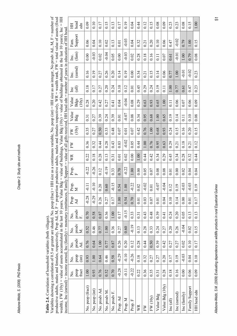
Alleb
one-
Web
b, S
. (20
08).
PhD
thes
is
C
hapte
r 2: S
tudy
site
and
met
hods
Alleb
one-
Web
b, S
.M. (
2009
) Eva
luatin
g de
pend
ence
on
wildl
ife p
rodu
cts in
rura
l Equ
ator
ial G
uinea
51
Tab
le 2
.4. C
orre
latio
n of
hou
seho
ld v
aria
bles
(bot
h vi
llage
s).
Var
iabl
es sh
owin
g a
corr
elat
ion
of 0
.5 o
r gre
ater
are
shad
ed. N
o. p
eop
(fra
c) =
HH
size
as a
con
tinuo
us v
aria
ble,
No.
peo
p (in
t) =
HH
size
as a
n in
tege
r, N
o pr
odv
Ad.
, M, F
= n
umbe
r of
prod
uctiv
e ad
ults
, mal
es a
nd fe
mal
es, r
espe
ctiv
ely,
Pro
p A
d, M
, F =
pro
porti
on p
rodu
ctiv
e ad
ults,
mal
es a
nd fe
mal
es re
spec
tivel
y, W
R =
wea
lth ra
nk, F
W =
tota
l val
ue o
f ass
ets
(fix
ed
wea
lth),
FW (1
0y) =
val
ue o
f ass
ets
accu
mul
ated
in th
e la
st 10
yea
rs, V
alue
Bdg
= v
alue
of b
uild
ings
, Val
ue B
dg (1
0y) =
val
ue o
f bui
ldin
gs o
btai
ned
in th
e la
st 10
yea
rs),
Inc
= H
H
inco
me,
Inc
(ear
ned)
= in
com
e ea
rned
, Inc
(fam
ily) =
mon
etar
y re
mitt
ance
s, Fa
mily
Sup
port
= va
lue
of a
ll gi
fts re
ceiv
ed, H
H h
ead
edn
= nu
mbe
r of y
ears
in e
duca
tion
of H
H h
ead.
No.
pe
op
frac
t
No.
pe
op
(int)
No.
pr
odv
Ad.
No.
pr
odv
M.
No.
pr
odv
F.
Prop
A
d Pr
op.
M
Prop
. F
WR
FW
FW
(10y
) V
alue
Bd
g V
alue
Bd
gs
(10y
)
Inc
(all)
In
c.
(ear
nd)
Inc.
(fa
m)
Fam
. Su
ppor
t H
H
head
ed
n N
o. p
eop
(frac
t) 1.
00
0.93
0.
76
0.52
0.
70
-0.2
8 -0
.11
-0.2
2 0.
22
0.36
0.
35
0.31
0.
28
0.18
0.
16
0.00
0.
06
0.09
N
o. p
eop
(int)
0.93
1.
00
0.64
0.
46
0.58
-0
.29
-0.1
0 -0
.26
0.18
0.
32
0.27
0.
27
0.20
0.
17
0.19
-0
.03
0.04
0.
10
No.
pro
dv A
d.
0.76
0.
64
1.00
0.
77
0.87
0.
26
0.20
0.
12
0.28
0.
44
0.50
0.
39
0.42
0.
27
0.27
0.
02
0.10
0.
17
No.
pro
dv M
. 0.
52
0.46
0.
77
1.00
0.
36
0.27
0.
60
-0.1
9 0.
13
0.28
0.
33
0.24
0.
27
0.20
0.
26
-0.0
4 0.
02
0.15
N
o. p
rodv
F.
0.70
0.
58
0.87
0.
36
1.00
0.
17
-0.1
5 0.
33
0.31
0.
43
0.48
0.
39
0.41
0.
24
0.20
0.
05
0.13
0.
13
Prop
. Ad
-0.2
8 -0
.29
0.26
0.
27
0.17
1.
00
0.54
0.
70
0.01
0.
03
0.07
0.
01
0.04
0.
10
0.14
0.
00
0.01
0.
17
Prop
. M
-0.1
1 -0
.10
0.20
0.
60
-0.1
5 0.
54
1.00
-0
.22
0.02
-0
.02
0.01
-0
.07
-0.0
4 0.
12
0.19
-0
.03
-0.0
3 0.
19
Prop
. F
-0.2
2 -0
.26
0.12
-0
.19
0.33
0.
70
-0.2
2 1.
00
0.00
0.
05
0.07
0.
08
0.08
0.
01
0.00
0.
02
0.04
0.
04
WR
0.22
0.
18
0.28
0.
13
0.31
0.
01
0.02
0.
00
1.00
0.
44
0.42
0.
34
0.29
0.
45
0.34
0.
28
0.32
0.
44
FW
0.36
0.
32
0.44
0.
28
0.43
0.
03
-0.0
2 0.
05
0.44
1.
00
0.76
0.
95
0.63
0.
29
0.21
0.
18
0.21
0.
12
FW (1
0y)
0.35
0.
27
0.50
0.
33
0.48
0.
07
0.01
0.
07
0.42
0.
76
1.00
0.
68
0.93
0.
24
0.15
0.
16
0.20
0.
15
Val
ue B
dg
0.31
0.
27
0.39
0.
24
0.39
0.
01
-0.0
7 0.
08
0.34
0.
95
0.68
1.
00
0.65
0.
19
0.14
0.
11
0.10
0.
08
Val
ue B
dg (1
0y)
0.28
0.
20
0.42
0.
27
0.41
0.
04
-0.0
4 0.
08
0.29
0.
63
0.93
0.
65
1.00
0.
11
0.06
0.
07
0.06
0.
09
Inc
(all)
0.
18
0.17
0.
27
0.20
0.
24
0.10
0.
12
0.01
0.
45
0.29
0.
24
0.19
0.
11
1.00
0.
77
0.61
0.
47
0.23
In
c (e
arne
d)
0.16
0.
19
0.27
0.
26
0.20
0.
14
0.19
0.
00
0.34
0.
21
0.15
0.
14
0.06
0.
77
1.00
-0
.01
-0.0
2 0.
23
Inc
(fam
ily)
0.00
-0
.03
0.02
-0
.04
0.05
0.
00
-0.0
3 0.
02
0.28
0.
18
0.16
0.
11
0.07
0.
61
-0.0
1 1.
00
0.79
0.
08
Fam
ily S
uppo
rt 0.
06
0.04
0.
10
0.02
0.
13
0.01
-0
.03
0.04
0.
32
0.21
0.
20
0.10
0.
06
0.47
-0
.02
0.79
1.
00
0.15
H
H h
ead
edn
0.09
0.
10
0.17
0.
15
0.13
0.
17
0.19
0.
04
0.44
0.
12
0.15
0.
08
0.09
0.
23
0.23
0.
08
0.15
1.
00
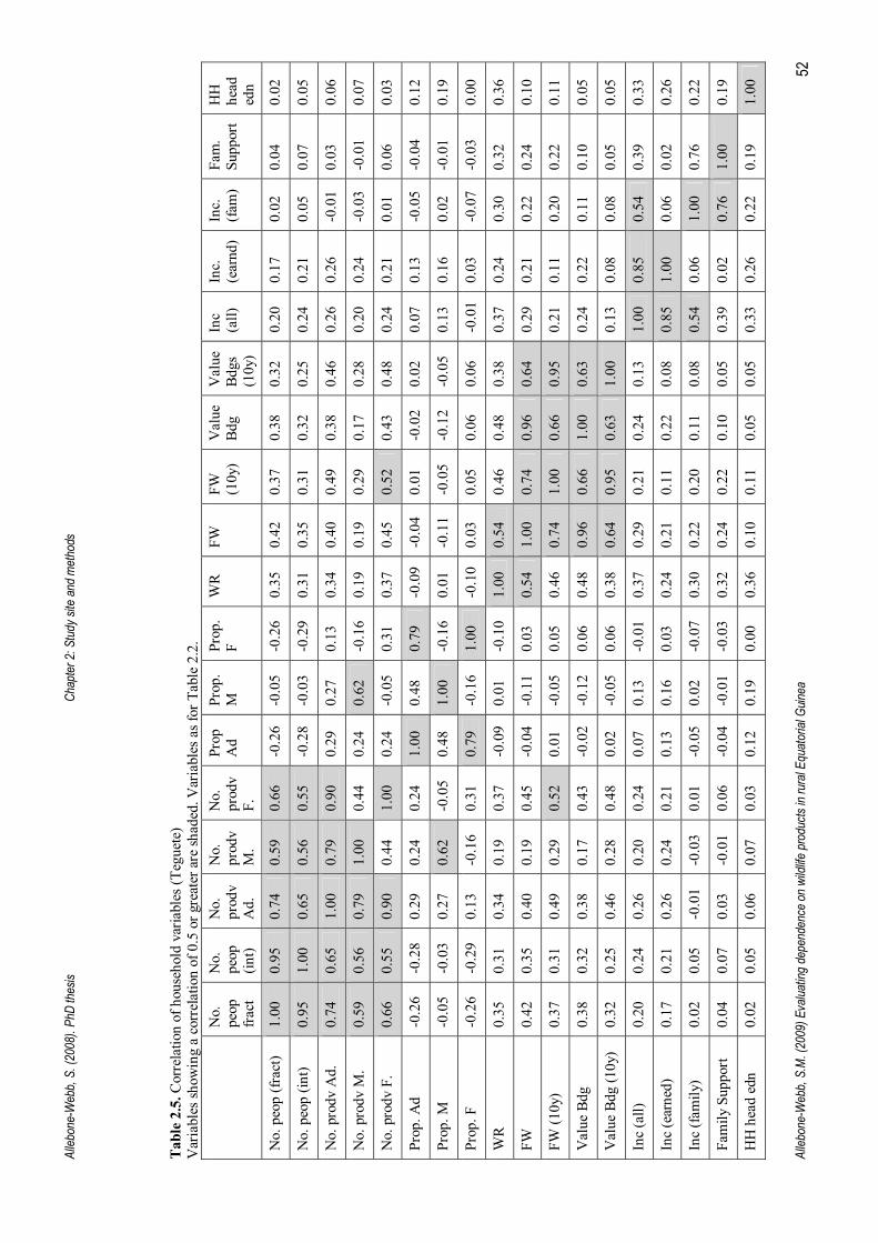
Alleb
one-
Web
b, S
. (20
08).
PhD
thes
is
C
hapte
r 2: S
tudy
site
and
met
hods
Alleb
one-
Web
b, S
.M. (
2009
) Eva
luatin
g de
pend
ence
on
wildl
ife p
rodu
cts in
rura
l Equ
ator
ial G
uinea
52
Tab
le 2
.5. C
orre
latio
n of
hou
seho
ld v
aria
bles
(Teg
uete
) V
aria
bles
show
ing
a co
rrel
atio
n of
0.5
or g
reat
er a
re sh
aded
. Var
iabl
es a
s for
Tab
le 2
.2.
N
o.
peop
fr
act
No.
pe
op
(int)
No.
pr
odv
Ad.
No.
pr
odv
M.
No.
pr
odv
F.
Prop
A
d Pr
op.
M
Prop
. F
WR
FW
FW
(10y
) V
alue
Bd
g V
alue
Bd
gs
(10y
)
Inc
(all)
In
c.
(ear
nd)
Inc.
(fa
m)
Fam
. Su
ppor
t H
H
head
ed
n
No.
peo
p (fr
act)
1.00
0.
95
0.74
0.
59
0.66
-0
.26
-0.0
5 -0
.26
0.35
0.
42
0.37
0.
38
0.32
0.
20
0.17
0.
02
0.04
0.
02
No.
peo
p (in
t) 0.
95
1.00
0.
65
0.56
0.
55
-0.2
8 -0
.03
-0.2
9 0.
31
0.35
0.
31
0.32
0.
25
0.24
0.
21
0.05
0.
07
0.05
No.
pro
dv A
d.
0.74
0.
65
1.00
0.
79
0.90
0.
29
0.27
0.
13
0.34
0.
40
0.49
0.
38
0.46
0.
26
0.26
-0
.01
0.03
0.
06
No.
pro
dv M
. 0.
59
0.56
0.
79
1.00
0.
44
0.24
0.
62
-0.1
6 0.
19
0.19
0.
29
0.17
0.
28
0.20
0.
24
-0.0
3 -0
.01
0.07
No.
pro
dv F
. 0.
66
0.55
0.
90
0.44
1.
00
0.24
-0
.05
0.31
0.
37
0.45
0.
52
0.43
0.
48
0.24
0.
21
0.01
0.
06
0.03
Prop
. Ad
-0.2
6 -0
.28
0.29
0.
24
0.24
1.
00
0.48
0.
79
-0.0
9 -0
.04
0.01
-0
.02
0.02
0.
07
0.13
-0
.05
-0.0
4 0.
12
Prop
. M
-0.0
5 -0
.03
0.27
0.
62
-0.0
5 0.
48
1.00
-0
.16
0.01
-0
.11
-0.0
5 -0
.12
-0.0
5 0.
13
0.16
0.
02
-0.0
1 0.
19
Prop
. F
-0.2
6 -0
.29
0.13
-0
.16
0.31
0.
79
-0.1
6 1.
00
-0.1
0 0.
03
0.05
0.
06
0.06
-0
.01
0.03
-0
.07
-0.0
3 0.
00
WR
0.35
0.
31
0.34
0.
19
0.37
-0
.09
0.01
-0
.10
1.00
0.
54
0.46
0.
48
0.38
0.
37
0.24
0.
30
0.32
0.
36
FW
0.42
0.
35
0.40
0.
19
0.45
-0
.04
-0.1
1 0.
03
0.54
1.
00
0.74
0.
96
0.64
0.
29
0.21
0.
22
0.24
0.
10
FW (1
0y)
0.37
0.
31
0.49
0.
29
0.52
0.
01
-0.0
5 0.
05
0.46
0.
74
1.00
0.
66
0.95
0.
21
0.11
0.
20
0.22
0.
11
Val
ue B
dg
0.38
0.
32
0.38
0.
17
0.43
-0
.02
-0.1
2 0.
06
0.48
0.
96
0.66
1.
00
0.63
0.
24
0.22
0.
11
0.10
0.
05
Val
ue B
dg (1
0y)
0.32
0.
25
0.46
0.
28
0.48
0.
02
-0.0
5 0.
06
0.38
0.
64
0.95
0.
63
1.00
0.
13
0.08
0.
08
0.05
0.
05
Inc
(all)
0.
20
0.24
0.
26
0.20
0.
24
0.07
0.
13
-0.0
1 0.
37
0.29
0.
21
0.24
0.
13
1.00
0.
85
0.54
0.
39
0.33
Inc
(ear
ned)
0.
17
0.21
0.
26
0.24
0.
21
0.13
0.
16
0.03
0.
24
0.21
0.
11
0.22
0.
08
0.85
1.
00
0.06
0.
02
0.26
Inc
(fam
ily)
0.02
0.
05
-0.0
1 -0
.03
0.01
-0
.05
0.02
-0
.07
0.30
0.
22
0.20
0.
11
0.08
0.
54
0.06
1.
00
0.76
0.
22
Fam
ily S
uppo
rt 0.
04
0.07
0.
03
-0.0
1 0.
06
-0.0
4 -0
.01
-0.0
3 0.
32
0.24
0.
22
0.10
0.
05
0.39
0.
02
0.76
1.
00
0.19
HH
hea
d ed
n 0.
02
0.05
0.
06
0.07
0.
03
0.12
0.
19
0.00
0.
36
0.10
0.
11
0.05
0.
05
0.33
0.
26
0.22
0.
19
1.00

Alleb
one-
Web
b, S
. (20
08).
PhD
thes
is
C
hapte
r 2: S
tudy
site
and
met
hods
Alleb
one-
Web
b, S
.M. (
2009
) Eva
luatin
g de
pend
ence
on
wildl
ife p
rodu
cts in
rura
l Equ
ator
ial G
uinea
53
Tab
le 2
.6. C
orre
latio
n of
hou
seho
ld v
aria
bles
(Bea
yop)
V
aria
bles
show
ing
a co
rrel
atio
n of
0.5
or g
reat
er a
re sh
aded
. Var
iabl
es a
s for
Tab
le 2
.2.
N
o.
peop
fr
act
No.
pe
op
(int)
No.
pr
odv
Ad.
No.
pr
odv
M.
No.
pr
odv
F.
Prop
A
d Pr
op.
M
Prop
. F
WR
FW
FW
(10y
) V
alue
Bd
g V
alue
Bd
gs
(10y
)
Inc
(all)
In
c.
(ear
nd)
Inc.
(fa
m)
Fam
. Su
ppor
t H
H
head
ed
n
No.
peo
p (fr
act)
1.00
0.
90
0.77
0.
40
0.76
-0
.33
-0.2
3 -0
.14
0.00
0.
28
0.31
0.
24
0.23
0.
10
0.13
-0
.06
0.06
0.
10
No.
peo
p (in
t) 0.
90
1.00
0.
62
0.31
0.
63
-0.3
3 -0
.20
-0.1
8 -0
.02
0.26
0.
21
0.21
0.
12
0.05
0.
14
-0.1
3 -0
.03
0.13
No.
pro
dv A
d.
0.77
0.
62
1.00
0.
71
0.82
0.
19
0.09
0.
14
0.14
0.
55
0.51
0.
48
0.39
0.
23
0.24
0.
00
0.18
0.
22
No.
pro
dv M
. 0.
40
0.31
0.
71
1.00
0.
19
0.33
0.
56
-0.2
5 0.
02
0.44
0.
38
0.37
0.
28
0.16
0.
26
-0.0
8 0.
03
0.18
No.
pro
dv F
. 0.
76
0.63
0.
82
0.19
1.
00
0.00
-0
.33
0.40
0.
18
0.42
0.
40
0.38
0.
32
0.19
0.
13
0.07
0.
23
0.16
Prop
. Ad
-0.3
3 -0
.33
0.19
0.
33
0.00
1.
00
0.67
0.
47
0.17
0.
17
0.17
0.
09
0.08
0.
15
0.15
0.
07
0.11
0.
27
Prop
. M
-0.2
3 -0
.20
0.09
0.
56
-0.3
3 0.
67
1.00
-0
.34
0.00
0.
10
0.08
0.
00
-0.0
3 0.
10
0.22
-0
.09
-0.0
8 0.
18
Prop
. F
-0.1
4 -0
.18
0.14
-0
.25
0.40
0.
47
-0.3
4 1.
00
0.22
0.
10
0.13
0.
11
0.14
0.
08
-0.0
6 0.
20
0.24
0.
13
WR
0.00
-0
.02
0.14
0.
02
0.18
0.
17
0.00
0.
22
1.00
0.
32
0.35
0.
20
0.20
0.
50
0.44
0.
23
0.30
0.
48
FW
0.28
0.
26
0.55
0.
44
0.42
0.
17
0.10
0.
10
0.32
1.
00
0.79
0.
94
0.63
0.
32
0.22
0.
14
0.18
0.
19
FW (1
0y)
0.31
0.
21
0.51
0.
38
0.40
0.
17
0.08
0.
13
0.35
0.
79
1.00
0.
73
0.92
0.
26
0.21
0.
10
0.15
0.
19
Val
ue B
dg
0.24
0.
21
0.48
0.
37
0.38
0.
09
0.00
0.
11
0.20
0.
94
0.73
1.
00
0.69
0.
18
0.05
0.
13
0.15
0.
17
Val
ue B
dg (1
0y)
0.23
0.
12
0.39
0.
28
0.32
0.
08
-0.0
3 0.
14
0.20
0.
63
0.92
0.
69
1.00
0.
10
0.04
0.
07
0.09
0.
16
Inc
(all)
0.
10
0.05
0.
23
0.16
0.
19
0.15
0.
10
0.08
0.
50
0.32
0.
26
0.18
0.
10
1.00
0.
65
0.67
0.
58
0.07
Inc
(ear
ned)
0.
13
0.14
0.
24
0.26
0.
13
0.15
0.
22
-0.0
6 0.
44
0.22
0.
21
0.05
0.
04
0.65
1.
00
-0.1
2 -0
.13
0.17
Inc
(fam
ily)
-0.0
6 -0
.13
0.00
-0
.08
0.07
0.
07
-0.0
9 0.
20
0.23
0.
14
0.10
0.
13
0.07
0.
67
-0.1
2 1.
00
0.88
-0
.10
Fam
ily S
uppo
rt 0.
06
-0.0
3 0.
18
0.03
0.
23
0.11
-0
.08
0.24
0.
30
0.18
0.
15
0.15
0.
09
0.58
-0
.13
0.88
1.
00
0.06
HH
hea
d ed
n 0.
10
0.13
0.
22
0.18
0.
16
0.27
0.
18
0.13
0.
48
0.19
0.
19
0.17
0.
16
0.07
0.
17
-0.1
0 0.
06
1.00

Chapter 3.
The consumption of wild
foods

Allebone-Webb, S. (2008). PhD thesis Chapter 3: The consumption of wild foods
Allebone-Webb, S.M. (2009) Evaluating dependence on wildlife products in rural Equatorial Guinea 55
3.1 Abstract
To assess the dependence on forest products, I begin with an analysis of the contribution of wild
foods to energy and protein consumption in two study villages. People in Teguete, the more rural
village, consumed more wild foods. Of these, bushmeat, followed by wild plants were more
important than wild fish. Wild foods in general were more important for protein consumption than
calorie intake, particularly because households obtained a lower proportion of their protein from
household production (agricultural and forest harvests), than calories. There was some increase in
bushmeat consumption with wealth, particularly for Beayop where consumption of bushmeat was
generally lower. The increased consumption of wild plants during the lean season may compensate
for lower calorie and protein consumption from agricultural harvests during this period in Teguete,
but there was no evidence of this in Beayop. The loss of wild food products to communities is
therefore most likely to impact protein consumption of the poorest households.
3.2 Introduction
The use of wildlife products is extremely widespread (Prescott-Allen & Prescott-Allen 1982;
Falconer 1990; de Beer & McDermott 1996), and traditionally the view has been that their
primary use is in the provision of food to local people. Consequently, in investigating the
dependence of people on wild foods, I begin with an analysis of the contribution of wild foods to
the diet; how often people eat different foods (wild and otherwise) and the contribution of these
foods to energy and protein consumption. I investigate differences in food sources (i.e. where and
how households have directly obtained foods) and in food types (i.e. agricultural, wild, coastal or
imported foods: the original source of these products) to give a thorough examination of the
importance of wild foods for macronutrients both directly (as households harvest foods from the
forest themselves), and indirectly (as determined by the amounts of wild foods eaten, regardless of
how obtained) in the two study villages.
3.2.1 Wild meat and fish
Wild meat and fish are most often cited as an important source of protein, as opposed to other
nutrients. Many people living in, or close to, tropical forests use meat as a major source of protein
(Bennett & Robinson 2000) and wildlife often supplies this meat and is the primary source of
protein for rural and urban households in many forested regions of poor nations (Redford & Kent
1993; Chardonnet et al. 1995; Juste et al. 1995; Ntiamoa-Baidu 1997), as well as being a source of
income. However, the consumption of all meat and fish, as well as wild meat and fish varies

Allebone-Webb, S. (2008). PhD thesis Chapter 3: The consumption of wild foods
Allebone-Webb, S.M. (2009) Evaluating dependence on wildlife products in rural Equatorial Guinea 56
considerably between country even within west and central Africa (Table 3.1), and between rural
and urban consumers, with the former often consuming more wild meat and fish than their urban
counterparts.
Table 3.1 Meat and fish consumption (including from wild sources) in west and central Africa, as reported in previous studies. Daily recommended amount of protein is 52g/ AME/day (FAO & WHO 1985).
Country Study population
Meat and fish consumption
Wild meat & fish consumption Reference
Cameroon Three rural communities
271-306g /AME/day
70-88% protein (and almost all meat and fish consumption)
(Koppert et al. 1993)
Equatorial Guinea
Urban consumers
385g /AME/day 20% protein (bushmeat only)
(Albrechtsen et al. 2005)
Equatorial Guinea
Total supply to capital city
2129.6 t/yr 1.5% protein (Albrechtsen et al. 2005)
Ghana Rural 33g/person/day (bushmeat only)
(Cowlishaw et al. 2007)
Ghana Urban 46g/person/day (bushmeat only)
(Cowlishaw et al. 2007)
Gabon Rural 268g/AME/day (bushmeat only) (16% of total value of consumed foods)
(Starkey 2004)
Central Africa Rural 130g/ person/day (bushmeat only)
(Wilkie & Carpenter 1999)
Central Africa Urban 13g/person/day (bushmeat only)
(Wilkie & Carpenter 1999)
Central African Republic
38% protein (Périssé 1966; Pondi et al. 1989), reported in (Koppert et al. 1993)
Cameroon Rural, southern Cameroon
70-88% protein as above
Cameroon Urban 27-57% protein as above
Côte d�Ivoire 25% protein as above
Congo 43% protein as above
Togo 20% protein as above
Gabon 59% protein as above
Uganda 9% protein as above
Nigeria 4% protein as above

Allebone-Webb, S. (2008). PhD thesis Chapter 3: The consumption of wild foods
Allebone-Webb, S.M. (2009) Evaluating dependence on wildlife products in rural Equatorial Guinea 57
Why people eat bushmeat, and how this varies across individuals, is still not well understood. Some
studies state it to be a luxury product that consumers will pay a premium for, noting its role in
ceremonies and as a reminder of village life for urban families (Chardonnet et al. 1995; Njiforti
1996). Other studies have tried to gauge a taste preference for different animal types, but have
shown only an inconsistent preference for bushmeat (only rural consumers consistently chose
bushmeat over domestic alternatives, Schenck et al. 2006), or a preference for fresh meat and fish of
all types (including bushmeat, but with fish being most preferred, East et al. 2005). There is other
evidence showing that most consumers respond to price, typically choosing the most affordable
meat or fish available (Bowen-Jones 1998; Wilkie & Carpenter 1999; Wilkie & Godoy 2000).
Consequently, the amount and proportion of different animal products eaten often varies with
household income, but again this differs between country, region and community (Table 3.2). This
may in part reflect differences in the range of wealth categories of the surveys in question, as well
as the price of, and preference for, each meat and fish type.
Table 3.2 Variation in meat and fish consumption (including from wild sources) with household wealth, as reported in previous studies.
Country/Region Study population Wealthier consumers consume: Reference
Equatorial Guinea
Rural More meat and fish (all types) No effect on bushmeat consumption
(Kümpel 2006)
Equatorial Guinea
Urban (Bata)
More bushmeat (possibly because it was the only fresh meat commonly available) More fresh fish
(East et al. 2005)
Equatorial Guinea
Urban (Malabo)
More fresh livestock Less bushmeat No effect on overall meat and fish consumption
(Fa et al. 2006)
DR Congo More fresh fish (de Merode et al. 2004)
South America Less bushmeat Less fish
(Wilkie & Godoy 2001)
Gabon Rural More bushmeat (although peaked with the third highest income quartile)
(Starkey 2004)
Gabon More meat (all types) More fresh fish
(Wilkie et al. 2005)
Meat and fish state may also affect consumer preference and price, and consequently consumption.
In Equatorial Guinea, frozen meat and fish were shown to be the cheapest animal meat types
(excluding smoked fish), but were least preferred, with consumption decreasing with increasing
income (East et al. 2005, and see Chapter 6). Smoking meat or fish can also affect price and
preference, and in Equatorial Guinea, smoked bushmeat is significantly cheaper than fresh meat and

Allebone-Webb, S. (2008). PhD thesis Chapter 3: The consumption of wild foods
Allebone-Webb, S.M. (2009) Evaluating dependence on wildlife products in rural Equatorial Guinea 58
smoked fish is the cheapest animal source all of (see Chapter 6), and is sometimes referred to as
�poor man�s food� (Kümpel 2006). In contrast, smoked bushmeat in Ghana commands a higher
price than fresh counterparts (Cowlishaw et al. 2005), probably due to the cost in time and money
(i.e. the cost of fuel) of smoking meat and the greater storage time of meat once smoked.
Evidence indicating that fish and bushmeat can be substitutes for each other in some regions is
mounting. In central and west Africa, fresh fish was preferred (East et al. 2005), and consumption
increased with income (see Table 3.2). In addition, Brashares et al (2004) show that bushmeat
consumption varies with fish availability and price in Ghana, while Wilkie et al (2005) show an
increase in fish consumption with increasing bushmeat prices in Gabon. In contrast, in South
America, fish is apparently an inferior good, with consumption decreasing with income (Wilkie &
Godoy 2001).
Other predictors of bushmeat, domestic meat and fish consumption and preference include ethnic
group (Fa et al. 2002; Kümpel 2006), with groups such as the Fang in Equatorial Guinea, having
stronger preferences for bushmeat; household size (Fa et al. 2006), with larger households eating
less total meat per AME in Malabo; gender (Koppert et al. 1993), with men generally eating
proportionally more meat and fish (as grams per total calories consumed), while women and
children eat proportionally more roots and tubers; and perhaps a weak variation in total calories
consumed with season (Koppert et al. 1993), with a decrease in calorie intake towards the end of the
main rainy season shown for one population in south Cameroon, but no differences in two other
populations, and no clear seasonal patterns over all. Another study gave stronger evidence for a
seasonal variation in bushmeat and fish consumption, with households eating more of these during
the lean season (de Merode et al. 2004).
Research therefore shows that the consumption of different categories of meat and fish can vary due
to price, preference (individual or cultural) and wealth of the consumer. In Equatorial Guinea at
least, consumers may differentiate between food state (i.e. whether fresh, frozen or smoked) far
more than they do between food categories (i.e. whether bushmeat, livestock, or fish).
Understanding the relationships between these may be further confounded by differences between
rural and urban areas, and by consumers preferring what they have grown used to.

Allebone-Webb, S. (2008). PhD thesis Chapter 3: The consumption of wild foods
Allebone-Webb, S.M. (2009) Evaluating dependence on wildlife products in rural Equatorial Guinea 59
3.2.2 Wild plants
The consumption of wild plants has often been overlooked in previous studies, and until relatively
recently has been given little consideration. Approximately 1,500 species of wild plants are
collected for consumption in central and west Africa (Chege 1994), and research, particularly under
the �Non-timber Forest Products� (NTFP) label, has now shown their importance. Wild plants are
now viewed by many to be important for the dietary and medical needs of poor forest people, and
are particularly thought of as a safety net or reserve food for times of hardship, during lean seasons
(Ogoye-Ndegwa & Aagaard-Hansen 2003; de Merode et al. 2004), as a �famine food� (Senaratne et
al. 2003; Shackleton & Shackleton 2004; Delacote 2007), in times of conflict (e.g. �night spinach�
Jamiya et al. 2007) and even as a response to disease epidemics (Balee 1992), most recently
HIV/AIDS (UNAIDS 1999). In other areas, wild plants are regularly consumed and harvested all
year round, and play a substantial role in diet and nutrition (Bhattacharya & Patra 2007; Bikoue &
Essomba 2007), particularly for women (Jimoh & Haruna 2007), as well as for income and
livelihoods (see Chapter 4). In addition, some have reported a positive link between health and wild
food consumption (Dounias & Colfer 2008), and in one case the bush mango, caused a decrease in
obesity and cholesterol in obese patients (Oben et al. 2008). Indeed, the role of NTFPs in Central
Africa has recently been highlighted by the FAO project �Enhancing food security through Non-
Wood Forest Products in Central Africa�.
There have been virtually no studies on the consumption of wild plants in Equatorial Guinea. A
preliminary market survey documents some of the species commonly traded (Sunderland & Obama
1998) and Cogels (1997) lists only a few wild food plants collected: palm nut (Elaeis guineensis),
palm wine (from various palm species), bush mango (Irvingia gabonensis), and wild fruit species
such as �metom� (Dacyodes macrophylia); as well as non-food plants: raffia, bamboo and
unspecified medicines, none of which appear to be sold. Significantly, Dounias (1993) noted that
wild plant harvest practices in neighbouring Cameroon were not observed in similar villages in
Equatorial Guinea, even in the Campo area, near to the Cameroon border, concluding that
traditional practices of forest plant product harvesting may have been lost in Equatorial Guinea.
Koppert et al (1996), however, showed a relatively low consumption of non-animal forest products
in Cameroon, mainly made up of mushrooms, wild yams, and some nuts and grains such as bush
mango, with the latter only present in July-August. They attribute this low value to the already
stretched time budget of women, who spend much of the day in the fields and kitchen. They do note
that men use more wild foods when on hunting trips and that these plants are mainly used for
flavouring rather than making a significant nutritional contribution, but that they add more protein
than calories.

Allebone-Webb, S. (2008). PhD thesis Chapter 3: The consumption of wild foods
Allebone-Webb, S.M. (2009) Evaluating dependence on wildlife products in rural Equatorial Guinea 60
This study has not examined the role of wild foods to micronutrition (i.e. the provision of vitamins
and minerals), but their contribution to consumption of micronutrients such as vitamins A and C,
iron, and dietary diversity in general has been noted, particularly for fruits and leafy greens
(Hoskins 1990; Ogden 1990), in urban as well as rural areas (Gockowski et al. 2003), and for
people living with HIV/AIDS (Barany et al. 2004). To highlight the importance that some ascribe to
wild plants, there is concern that exotic introductions of alternative leafy vegetables (e.g. Brassica
spp.) and the subsequent reduction in native, wild plants, may cause a loss in nutritional intake,
particularly among the poor, if introduced species have lower nutritional values, cause a narrowing
of harvests or a loss of local knowledge for harvest and production of these vegetables (FAO 1988;
Udosen 1995; Okafor 1997; Future-Harvest 2001).
Fuelwood may actually be one of the most important NTFPs for household nutrition. Fuelwood
makes up 61-86% of the primary energy consumption in some regions of Africa, of which 74-97%
is used by households (Amous 2000). Fuel availability can determine the nutritional value of meals
(Egal et al. 2000), as cooking releases nutrients in grains and fibrous roots, and some staples such as
cassava can be toxic without such processing.
3.2.3 Wild invertebrates and herpetiles
The consumption of edible insects such as caterpillars, larvae and crickets, snails, other
invertebrates, and small herpetiles such as frogs has been studied in many cases, although again is
often neglected by studies and particularly by regulatory frameworks and development assistance
(de Foliart 1999; Vantomme et al. 2004; Nasi et al. 2008). Insects are a popular food source in
many countries, whether for regular consumption, as an occasional delicacy, or as a safety net eaten
in times of food shortages, and estimates suggest that more than 1,000 species of terrestrial
invertebrates are consumed by people (de Foliart 1992; Marconi et al. 2002; Vantomme et al. 2004).
Studies have shown that insects can contribute significantly to the diets of the rural poor, for daily
fat, protein, vitamin and mineral requirements (de Foliart 1992; Illgner & Nel 2000). Marconi et al
(2002) showed that consumption of 100g of invertebrates contributed 1.2-9.4% of daily fat
requirements and 6-144% of daily protein requirements in Amazonia. Other research has shown that
caterpillars have higher protein and fat content than meat or fish (Malaisse 1997) and that some
species are very rich in vitamins and/or minerals (de Foliart 1992). Indeed, de Foliart (1992)
showed that 100g of caterpillars could provide 100% of the daily requirements of the contained
vitamins and minerals.

Allebone-Webb, S. (2008). PhD thesis Chapter 3: The consumption of wild foods
Allebone-Webb, S.M. (2009) Evaluating dependence on wildlife products in rural Equatorial Guinea 61
3.2.4 Food sources and food types
There are few data on the actual origin of bushmeat consumed in households, so it is difficult to
know how much is directly harvested by households, and how much is traded within villages and in
informal markets. In Equatorial Guinea, one study in urban Malabo showed that 97% of bushmeat
consumed was bought and 3% received as gifts (Albrechtsen et al. 2005), while in a rural village,
over half of bushmeat consumed was captured by the household itself (Kümpel 2006).
In this chapter, I assess the contribution of different food types by dividing foods into categories,
regardless of how they were obtained by the household (i.e. all foods originally gained from the
forest, foods imported into the country, agricultural foods, etc.) to examine the contribution of these
foods to the community as a whole, as well as the differences in consumption patterns between
individuals and communities in both villages. In a different set of analyses, I assess the contribution
of different food sources by categorising foods consumed according to how they were obtained by
the household (i.e. wild foods obtained from the forest by the household in question, items bought,
food received as a gift, and food produced in the fields), to determine the direct contribution of the
forest for individuals and households. Given previous research outlined above, I hypothesise that:
1) More remote communities (i.e. Teguete) will consume more wild foods;
2) Medium or wealthier households will consume more meat and fish in general, and
specifically more bushmeat and wild fish;
3) Poorer households and women will consume more wild plants;
4) Poorer households will consume more items directly sourced themselves (either from forest
or agriculture), while richer households will consume more bought items;
5) The consumption of wild products will be highest in the hungry season.
3.3 Methods
3.3.1 Data Collection
During the regular household interviews (see Chapter 2), households in each village were visited
approximately every fortnight. All adults in the household were asked about their food consumption
during the previous day and the consumption by children in the household, and an interview was
deemed invalid if any household member over 18 could not be found or their answers not recorded.
The household member who had cooked was asked about the ingredients of any food prepared, and
all respondents asked a series of questions taking them through the day�s consumption (i.e. asking
what they ate first thing, then what they ate, etc.), and including food and drinks eaten in the house,

Allebone-Webb, S. (2008). PhD thesis Chapter 3: The consumption of wild foods
Allebone-Webb, S.M. (2009) Evaluating dependence on wildlife products in rural Equatorial Guinea 62
in other peoples houses, in the fields, bought in the street or in bars, and who was present for each
eating event (including guests), following methods laid out by Swindale & Ohri-Vachaspati (1999).
For each food item, questions were asked on how many times it was eaten the previous day, how
the food was obtained (bought, received as a present, harvested from the fields, trapped or hunted,
etc.), where obtained from (bought in a bar in the village, an urban market or wholesalers, a local
fisherman, etc), in what state it was obtained (fresh, smoked, frozen, rotten), when obtained, what
quantity obtained, and for what price. Fang or local names of forest animals, fish and wild plants
were used to avoid misidentification.
Respondents were asked about the quantity of food consumed using local units, and the weight of
the same amount of food measured using the same container where possible. Additional data was
also collected on the weights of different food types of different states in different local units
wherever possible. Common units included: handful (amount filling one palm), double handful
(amount filling two palms), wicker dish (locally made), small, medium and large saucepans, locally
made wicker baskets used to transport food harvested from fields, and entire unit of something (e.g.
a whole banana). When weighing items, care was taken to note the state of the food (i.e. raw,
cooked, smoked, etc.), whether or not it was peeled or skinned, which household it was weighed in,
and to note any equivalent units (i.e. the number of entire avocados in one basket). For foods that
were prepared and eaten over more than one day (e.g. when a pot of food was cooked and then half
of it eaten one evening, and the remainder eaten for the following breakfast or lunch), the amount
consumed for the sample day alone was estimated from the total quantity, based on the number of
times it was eaten over both days and the number of people eating at each event.
Where a food item was weighed during the interview, that weight was used in all calculations.
Where food was not weighed during an interview, the average weight for that food, state and unit
for that household was taken. Where these data were not available, the average weight of that food,
state and unit for the village was taken. Where possible, the estimated calorie and protein amounts
per kilo of foods were taken from Cooperacion Sanitaria Española con Guinea Ecuatorial (1991)
which contains country-specific values of common and local foods. Otherwise nutritional values
were taken from various sources, including FAO (1997).
Daily food consumption per household was taken by adding the estimated calorie and protein
amounts for each food item and amount eaten that day. To calculate individual consumption, the
amounts of food items that were eaten from a shared pot were proportioned according to the Adult
Male Equivalent (AME) of all the people eating that food and the values added for each person.
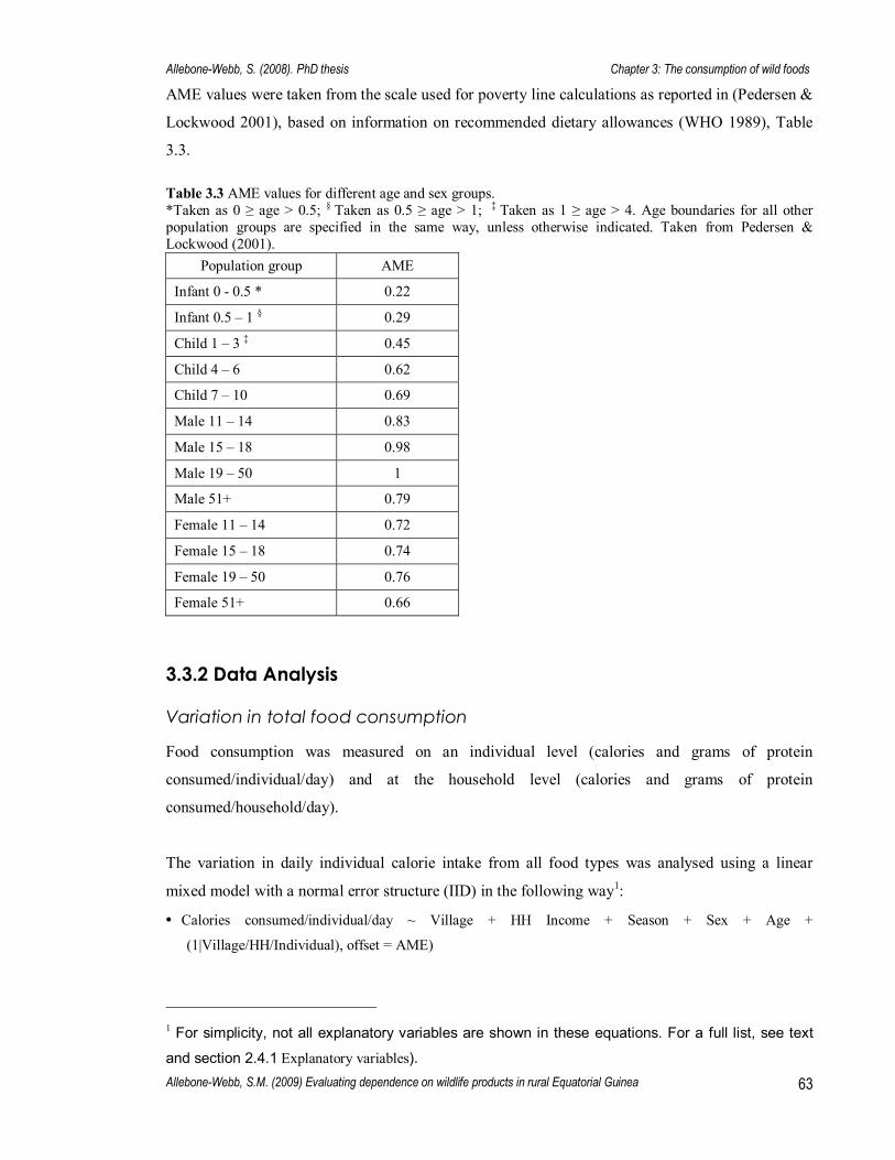
Allebone-Webb, S. (2008). PhD thesis Chapter 3: The consumption of wild foods
Allebone-Webb, S.M. (2009) Evaluating dependence on wildlife products in rural Equatorial Guinea 63
AME values were taken from the scale used for poverty line calculations as reported in (Pedersen &
Lockwood 2001), based on information on recommended dietary allowances (WHO 1989), Table
3.3. Table 3.3 AME values for different age and sex groups. *Taken as 0 ≥ age > 0.5; § Taken as 0.5 ≥ age > 1; � Taken as 1 ≥ age > 4. Age boundaries for all other population groups are specified in the same way, unless otherwise indicated. Taken from Pedersen & Lockwood (2001).
Population group AME
Infant 0 - 0.5 * 0.22
Infant 0.5 � 1 § 0.29
Child 1 � 3 � 0.45
Child 4 � 6 0.62
Child 7 � 10 0.69
Male 11 � 14 0.83
Male 15 � 18 0.98
Male 19 � 50 1
Male 51+ 0.79
Female 11 � 14 0.72
Female 15 � 18 0.74
Female 19 � 50 0.76
Female 51+ 0.66
3.3.2 Data Analysis
Variation in total food consumption
Food consumption was measured on an individual level (calories and grams of protein
consumed/individual/day) and at the household level (calories and grams of protein
consumed/household/day).
The variation in daily individual calorie intake from all food types was analysed using a linear
mixed model with a normal error structure (IID) in the following way1:
• Calories consumed/individual/day ~ Village + HH Income + Season + Sex + Age +
(1|Village/HH/Individual), offset = AME)
1 For simplicity, not all explanatory variables are shown in these equations. For a full list, see text
and section 2.4.1 Explanatory variables).

Allebone-Webb, S. (2008). PhD thesis Chapter 3: The consumption of wild foods
Allebone-Webb, S.M. (2009) Evaluating dependence on wildlife products in rural Equatorial Guinea 64
The individual quantities of food eaten in the shared pot were estimated by dividing the total pot
amount by the number people eating it, proportionally to their Adult Male Equivalent (AME; see
Table 3.3 for AME values used). Given that the majority of food was consumed by the entire
household from a shared pot, there was only a small amount of variation between individual
household members, mainly made up of any snacks eaten outside of the home. Differences in
consumption from within the shared pot were not possible to detect with the data collected, and
given the communal nature of peoples� eating habits (people often eat literally from the same pot or
dish), this may only be possible using extremely labour intense and intrusive methods such as direct
observation. Condiments and small food items contributing minimally to nutrition (e.g. salt, chilli,
stock cubes and garlic) were not included in any analyses. Similarly, children under 2.5 were
excluded from all analyses.
Differences in calorie consumption with individual and household variables, season and village
were analysed. Household level variables were: household (HH) income, HH fixed wealth, HH
wealth rank, HH size, number of productive adults (aged 18-65 and not including the chronically
ill), number of productive females, presence/absence of productive males, proportion of productive
adults to total household size, proportion of productive females, education level of the HH head,
and gender of the HH head (see Chapter 2 for details). Individual level variables were: education,
sex and age. All variables were tested for normality and transformed where necessary.
Individuals nested within households, nested within villages (1|Village/HH/Individual) were
specified as random effects for analyses of individual consumption. Individual consumption was
offset by AME (adult Male Equivalent), effectively analysing differences in daily consumption per
AME. In other words, the calorie consumption per individual is measured against the expected
calorie consumption for that individual, according to their sex and age (see Table 3.3 for AME
values used).
The model was simplified to obtain the minimum adequate model (MAM) by fitting the saturated
(unrestrained) model and then comparing models with progressively simplified fixed effects using
change in deviance tests. Significance was taken as p<0.05.
Variation in protein consumption from all food types was analysed in the same way2:
• Protein consumed/individual/day ~ Village + HH income + Season + Sex + Age +
(1|Village/HH/Individual), offset = AME)
In order to ensure that any differences at the household level were still detectable without the need
to use figures derived from estimates based on AME and the distribution of a shared pot., variations

Allebone-Webb, S. (2008). PhD thesis Chapter 3: The consumption of wild foods
Allebone-Webb, S.M. (2009) Evaluating dependence on wildlife products in rural Equatorial Guinea 65
in household level calorie and protein consumption were similarly analysed, but with no offset for
AME and the random effects were specified as household nested with village (1|Village/HH) 2:
• Calories consumed/HH/day ~ Village + HH income + Season + No. Adults eating + No. children eating +
(1|Village/HH), offset = AME)
• Protein consumed/HH/day ~ Village + HH income + Season + No. Adults eating + No. children eating +
(1|Village/HH), offset = AME)
In these analyses, individual level variables were not included and the number of adults and number
of children eating at that household at that day were specified as addition explanatory variables, to
account for differences in household size.
Variation in consumption of different food types and from different food
sources
Food consumption was then divided into categories of food type and food source. Food type was
taken as the supply origin of that food type, and used to assess the contribution of different food
supplies to the community as a whole. Food source was taken as the means by which each food
item was obtained by the household, to analyse specifically how households obtain food. So, a bar
of cassava bought by a household would have food type �agriculture�, but food source �bought�.
Food type was divided into these categories:
• Agriculture � agricultural food items produced in the country, including cassava, peanuts and
almost all fresh fruit and vegetables
• Imports � food mainly imported into the country, including all processed foods (no processing
is done in Equatorial Guinea except one brand of beer not found in either village), such as all
tinned and packaged goods, frozen fish and meat, and agricultural goods not grown in
Equatorial Guinea (e.g. rice)
• Coastal � marine fish from the Rio Muni coast (and so part of the country�s food production).
All marine fish in the village was smoked.
• Wild � all non-cultivated species harvested from the forest, farm-fallow or agricultural land.
These were further split for additional analysis into:
• animal � terrestrial and bird wild animals (bushmeat)
• fish � all wild freshwater fish
• plant � forest plant products
2 For simplicity, not all explanatory variables are shown in these equations. For a full list, see
section 2.4.1 Explanatory variables).

Allebone-Webb, S. (2008). PhD thesis Chapter 3: The consumption of wild foods
Allebone-Webb, S.M. (2009) Evaluating dependence on wildlife products in rural Equatorial Guinea 66
These categories also reflect the geographical origins of the food types, with virtually all
agricultural and wild food being harvested locally, so if it was purchased it was almost always from
another household within the village. Some food items at times fell into either of two groups. The
most problematic of these was palm oil and other palm products, which were both cultivated in
fields and collected from wild growing trees in the forest. Although no oil palm plantations exist,
when a new field is cleared, if the area contains a palm tree it is usually left to grow and the palm
fruits harvested accordingly. Consequently, although a large proportion of oil products was
recorded as being harvested from the forest (~40%), a greater proportion was recorded as coming
from agricultural land (~60%), and so all palm products were classified as food type agriculture,
leading to a potential over estimation of the contribution of agricultural products and
underestimation of wild products3. Similarly difficult products to define were two classes of fish.
The fang words �bifaka� and �celele� are generic terms for small and smaller fish. These small fish
make up the majority of the small smoked fish brought from the coast, but small locally caught fish
can also be called by these terms, and if smoked, there is no way to know if they came from the
coast or were locally caught. To err on the side of caution, all smoked bifaka and celele were
classified as coastal, while fresh bifaka and celele were classified as wild (no fresh fish came from
Bata). Other locally caught fish had fang names specific to fresh water species, so there were no
problems in classifying these.
The calorie and protein contribution to consumption from each of these food types was analysed
against the explanatory variables above. Individual variation in daily calories consumed from
produced food as a proportion of the total calories consumed was analysed as above, using a mixed
model with a normal error structure, maximum likelihood method and offset by individual AME.
The proportion of calories from produced food was transformed by an arc sin transformation and
analysed against the explanatory variables above, transformed where necessary. Due to the large
number of zeros in the data and the consequent lack of a normal distribution, only days where some
of the food source in question was consumed were analysed, thus analysing the relationship of the
proportion of energy from a source only when it was being consumed. Variation in individual
protein consumption from produced food was analysed in the same way. The proportion of calories
or protein consumed was taken as the dependent variable rather than the absolute amounts
consumed, to give a greater reflection of the contribution to current diets, and to avoid distortions
caused by the large differences in activity levels and subsequent energy needs between different
groups (particularly between wealth categories). 3 The food source of palm products was still taken as the actual origin from which households had obtained it,
so included both �agriculture� and �forest� categories.

Allebone-Webb, S. (2008). PhD thesis Chapter 3: The consumption of wild foods
Allebone-Webb, S.M. (2009) Evaluating dependence on wildlife products in rural Equatorial Guinea 67
Food source was divided into these categories:
• Bought � food bought by a member of the household
• Agriculture � food produced by a member of the household, including food harvested from
fields by household members and any domestic animals eaten
• Gift � food received by household members as a gift
• Forest � food hunted, fished or gathered by household members. This included all non-
cultivated species collected from forests, fallow land and agricultural land. This group was
further split into:
• animals � all terrestrial and bird forest animals
• fish � wild caught fish (there were no reared fish or aquaculture in either village)
• plants � all forest plant foods
The frequency of consumption from each of these sources was separately analysed, with daily
presence or absence of each food source for each individual on each sample day given as a binomial
variable, using a mixed model with a binomial error structure, against the explanatory variables
above (transformed where necessary). In order to ascertain the different contributions of food
harvested from the forest, these were further divided into terrestrial animals, fish and plants.
As above, calorie and protein consumption from each of these food sources was analysed
individually against the explanatory variables. As with food types, the proportion of calories and
protein consumed from agricultural products was treated as a continuous variable, but due to data
limitations, the consumption of imported, coastal and wild foods on any sample day was treated as a
binary variable, followed by analysis of the proportion of calories and protein only for days where
that food type was consumed. All data were analysed in R, version 2.6.2 (R Development Core
Team 2007), using the lme4 library (Bates & Sarkar 2007).
3.4 Results
3.4.1 Total food consumption
People ate an average of 1534 calories per AME in Beayop and 1325 in Teguete which is lower
than the daily recommended amounts of 20004. Conversely, an average 66g of protein per day per
AME was consumed in Beayop and 61g in Teguete, which is higher than the daily recommended
4 Extreme caution should be shown when using daily recommended amounts of food intake, as people�s needs
vary so greatly. In addition, any estimates of food intake are likely to be underestimates.

Allebone-Webb, S. (2008). PhD thesis Chapter 3: The consumption of wild foods
Allebone-Webb, S.M. (2009) Evaluating dependence on wildlife products in rural Equatorial Guinea 68
amount of 52g/AME/day (FAO & WHO 1985). There is no significant difference in food
consumption between males and females (Figure 3.1, Figure 3.2), although females have slightly
higher calorie consumption per AME (although still a lower absolute calorie consumption).
As we would hope, the models at household and individual levels show very similar results,
suggesting that they reflect genuine differences between groups, as opposed to being an artefact of
AME calculations (Table 3.4). Individual calorie consumption, and household and individual
protein consumption, are significantly higher in Beayop (Figure 3.1, Figure 3.2). Household and
individual consumption of calories and protein increases significantly with wealth, as represented
by HH income or fixed wealth, and oppositely consumption of calories and protein decreases
significantly with household size. Individual consumption of calories and protein per AME
increases significantly with the proportion of productive females in the household and increases
significantly with age (Table 3.4), reflected in a higher recorded consumption of calories and
protein in over 18 year-olds (Figure 3.1, Figure 3.2). Seasonally, calorie consumption was lowest in
the 3rd season, followed closely by the 2nd season, and protein consumption was lowest in the 2nd
and 3rd seasons. Consumption of both calories and protein was highest in the 4th season.
Figure 3.1 Daily calorie consumption per AME for adults and children by gender and village
0
200
400
600
800
1000
1200
1400
1600
1800
Male Female Male Female Male Female Male Female
<18 18+ <18 18+
Beayop Teguete
Village, age and gender
Ave
rage
dai
ly c
alor
ie in
take
per
AM
E

Allebone-Webb, S. (2008). PhD thesis Chapter 3: The consumption of wild foods
Allebone-Webb, S.M. (2009) Evaluating dependence on wildlife products in rural Equatorial Guinea 69
Figure 3.2 Daily protein consumption per AME for adults and children by gender and village
0
10
20
30
40
50
60
70
80
Male Female Male Female Male Female Male Female
<18 18+ <18 18+
Beayop Teguete
Village, age and gender
Ave
rage
dai
ly p
rote
in in
take
per
AM
E (g
)
Table 3.4 Results of GLMMs � total energy and protein consumption from all foods. Significance and direction of trends are indicated by symbols: 1 symbol = p < 0.05; 2 symbols = p < 0.01; 3 symbols = p < 0.001. For significant multilevel categorical variables, differences between levels are indicated by symbols. A blank cell indicates no significant relationship. Explanatory variables that were not significant for any of the tested parameters were not included in the table. See Table A 5.1, Table A 5.2, Table A 5.3 and Table A 5.4 for details.
Variable Level
HH calorie consumption
Individual calorie consumption
HH protein consumption
Individual protein consumption
Season 1Small Dry 2 First Wet 3 Big Dry 4 Second Wet
+ - - ++
+ - - - +
+ - - ++
+ - - +
Village Beayop Teguete
+ -
+ -
+ -
HH Income + +
HH Fixed Wealth +++ +++ +++ +++
HH size - - - - - - - - - -
Proportion productive females
+++ +
Age NA +++ NA +++

Allebone-Webb, S. (2008). PhD thesis Chapter 3: The consumption of wild foods
Allebone-Webb, S.M. (2009) Evaluating dependence on wildlife products in rural Equatorial Guinea 70
3.4.2 The contribution of food types to consumption
General description of food types
Agriculture
Few livestock animals were reared in either village (see Chapter 4 for numbers), and even fewer
consumed (recorded consumed on less than 10 HH survey days), tending to be reserved for special
occasions, so virtually all produced foods were arable agricultural crops. Aside from food staples
such as cassava and plantains, the two main crops are peanuts and calabaza. Both are good sources
of protein and are used as a sauce eaten with meat, fish or greens, or as a meal in their own right, as
opposed to an accompaniment. However, plant-based protein is generally regarded as inferior, and
there is a strong preference for meat and fish, together with a belief that meat and fish are better for
the health.
Imported foods
The large amount of relatively cheap frozen meat and fish found in Bata does get transported to
some rural villages, either by enterprising village shop owners (as is the case in Beayop), although a
freezer and electricity generator are necessary for this, or may be sent in small quantities (usually
only for special occasions) to villages by family members living in the cities. The lack of a way to
store frozen food means that smaller or more remote villages do not usually have a regular supply
of frozen fish and domestic meat, and this is the case in Teguete.
Coastal
Small, smoked marine fish seem to reach virtually all rural villages in Río Muni, and this is true of
Beayop and Teguete. Most of this fish is caught off the shore of Río Muni, the bulk coming from
Cogo and the coastline between the southern border with Gabon and Bata, where it is usually
smoked and then transported to Bata. Village traders and other villagers visiting Bata or other cities
often buy (or get given) a plastic bag full of smoked fish and this can be stored in the village for
regular consumption or for sale in small portions of two to four fish to other villagers. This was the
cheapest animal protein available in either village.
Wild foods (forest foods)
Although no urban traders visited Beayop or Teguete specifically, hunters in both villages did
sometimes sell their products to other villagers, as well as to passing cars or traders, so a sizeable
proportion of bushmeat consumed was not directly captured by the household. Some hunters also
chopped up their catch, selling smaller, more affordable, portions of fresh bushmeat for around
500cfa. Wild fish and plants were also sold within the village, but on a far lower scale.

Allebone-Webb, S. (2008). PhD thesis Chapter 3: The consumption of wild foods
Allebone-Webb, S.M. (2009) Evaluating dependence on wildlife products in rural Equatorial Guinea 71
Community differences in consumption from different food types
In both villages, agricultural products were consumed virtually every day (Figure 3.3) and overall
provided the greatest proportion of calories of all food types (60% and 68% for Beayop and Teguete
respectively, Table 3.5). They were more important in Teguete, providing a significantly higher
proportion of protein and calories to households (Table 3.7). Households ate imported goods
significantly more often in Beayop, and these provided the highest proportion of protein of all food
types (41%). In Teguete forest products provided the majority of protein (53%), and were consumed
significantly more often and provided a significantly higher proportion of energy and protein when
they were consumed (Figure 3.3 and Table 3.7). Within forest products, bushmeat was most
important for protein provision in both villages, although it provided on average over twice the
protein to people in Teguete than in Beayop (Table 3.5), and was eaten significantly more often in
Teguete (Table 3.8). Wild plants provided the greatest overall proportion of calories of all forest
products in Teguete, and were eaten more often and provided a greater proportion of calories when
they were consumed. Forest fish provided a relatively small proportion of calories and protein to
households, but of this, it was more important in Beayop, providing a significantly higher
proportion of protein when it was consumed. Coastal food was eaten more frequently and provided
more energy and protein to households in Beayop, but this was lowest contributor of all food types.
Large proportions of the agricultural and forest products consumed were harvested directly by the
household, and in these cases the food type reflects the food source. For example, of the average
920 cal/AME/day gained from all agricultural products in Beayop, and 891cal/AME/day in Teguete
(Table 3.5), an average 773 cal/AME/day and 741 cal/AME/day respectively were obtained from
agricultural sources (

Allebone-Webb, S. (2008). PhD thesis Chapter 3: The consumption of wild foods
Allebone-Webb, S.M. (2009) Evaluating dependence on wildlife products in rural Equatorial Guinea 72
Table 3.9), giving an estimated 84% and 83% of agricultural products consumed in the household
that are harvested directly by the household in question (Table 3.6). In this way, the results show
that while a greater proportion of forest products consumed were harvested by the household in
Teguete, households were marginally more likely to buy or receive bushmeat as a gift in Teguete
than in Beayop (Table 3.6). The majority of forest fish and plants consumed in Teguete were
harvested directly by the household, while in Beayop most wild fish and plants consumed were
bought or received as a gift.
Table 3.5 Average contribution to calories and protein by different food types.
Food type Average calories/AME/day % total calories Average g
protein/AME % total protein consumption
Beayop Teguete Beayop Teguete Beayop Teguete Beayop Teguete
Agriculture 919.7 891.0 59.9 67.5 17.6 18.7 26.0 31.9
Import 474.0 135.3 30.9 10.3 28.0 6.3 41.3 10.8
Coastal 28.3 15.8 1.8 1.2 4.8 2.7 7.1 4.6
Forest products 112.3 277.8 7.3 21.0 17.4 30.9 25.7 52.7
Forest animals 61.8 123.9 4.0 9.4 12.3 25.0 18.1 42.7
Forest fish 27.5 7.1 1.8 0.5 4.5 1.4 6.6 2.4
Forest plants 23.0 146.8 1.5 11.1 0.6 4.5 0.9 7.7
Table 3.6 Average percentage of agricultural and forest foods consumed that were harvested directly by the household for each village. Figures were estimated using the average number of calories obtained of that food source, as a proportion of all calories of that food type consumed.
Food type Beayop Teguete
Agriculture 84.1 % 83.2 %
Forest (all) 51.7 % 71.0 %
Forest animals 65.1 % 56.7 %
Forest fish 26.8 % 76.6 %
Forest plants 45.7 % 82.8 %

Allebone-Webb, S. (2008). PhD thesis Chapter 3: The consumption of wild foods
Allebone-Webb, S.M. (2009) Evaluating dependence on wildlife products in rural Equatorial Guinea 73
Figure 3.3 Frequency of consumption of different food types
0
0.1
0.2
0.3
0.4
0.5
0.6
0.7
0.8
0.9
1
Beayop Teguete
Village
Prop
ortio
n of
day
s ea
ten
AgricultureImportCoastalWildPlantWildAnimalWildFish
Household variation in consumption from different food types
Individuals from wealthier households gained significantly lower proportions of energy and protein
from agriculture in both villages (Figure 3.4 and Table 3.7). Instead, wealthier households gained
more calories and protein from imported foods, and ate these significantly more frequently, as did
households with better educated household heads (Table 3.7). Wealthier households gained slightly
more protein and calories from coastal foods, and these were eaten most frequently by households
with a higher proportion of productive females, and with the most educated household heads. In
Beayop, wealthier households gained a higher proportion of calories and protein from forest foods,
while in Teguete, the poorest and wealthiest gained most from forest foods, driven by a
significantly greater frequency of consumption among the 1st and 4th wealth ranks. This increased
frequency of forest product consumption at the wealth extremes was probably due to wealthier
households eating wild plants most often in Beayop and poorer households eating them most often
in Teguete. Larger households also ate bushmeat significantly more often.

Allebone-Webb, S. (2008). PhD thesis Chapter 3: The consumption of wild foods
Allebone-Webb, S.M. (2009) Evaluating dependence on wildlife products in rural Equatorial Guinea 74
Figure 3.4 Average proportion of a) calories and b) protein for food types with wealth rank and village.
Seasonal variation in consumption from different food types
In both villages, agriculture provided the lowest proportions of calories from agriculture in the 2nd
season, and the lowest proportion of protein in the 2nd and 3rd seasons (Figure 3.5 and Table 3.7). In
compensation, the forest provided significantly higher proportions of calories and protein in the 2nd
and 3rd seasons in Teguete due to a higher frequency of consumption and higher proportion of
calories when they were consumed. Of these, forest plants were consumed most often and provided
the highest proportion of calories and protein in the 2nd and 3rd seasons in Teguete (Figure 3.5 and
Table 3.8), but bushmeat was consumed the least frequently, providing the lowest proportion of
0
0.1
0.2
0.3
0.4
0.5
0.6
0.7
0.8
0.9
1
1 2 3 4 1 2 3 4
Beayop Teguete
Village and wealth rank (1 = poorest)
Prop
ortio
n of
cal
orie
s ea
ten
WildFishWildAnimalWildPlantCoastalImportAgriculture
0
0.1
0.2
0.3
0.4
0.5
0.6
0.7
0.8
0.9
1
1 2 3 4 1 2 3 4
Beayop TegueteVillage and wealth rank (1 = poorest)
Prop
ortio
n of
pro
tein
eat
en
WildFishWildAnimalWildPlantCoastalImportAgriculture
a)
b)

Allebone-Webb, S. (2008). PhD thesis Chapter 3: The consumption of wild foods
Allebone-Webb, S.M. (2009) Evaluating dependence on wildlife products in rural Equatorial Guinea 75
protein in the 2nd season. Seasonal differences in consumption of forest products in Beayop were
less varied, except for wild fish which were eaten most frequently and provided most protein in the
4th season. Figure 3.5 Graphs showing average proportions of a) protein and b) calories consumed from food types with village and season.
0
0.1
0.2
0.3
0.4
0.5
0.6
0.7
0.8
0.9
1
1Litt
leD
ry
2Firs
tWet
3Big
Dry
4Sec
ondW
et
1Litt
leD
ry
2Firs
tWet
3Big
Dry
4Sec
ondW
et
Beayop TegueteVillage and Season
Prop
ortio
n of
cal
orie
s ea
ten
WildFishWildAnimalWildPlantCoastalImportAgriculture
0
0.1
0.2
0.3
0.4
0.5
0.6
0.7
0.8
0.9
11L
ittle
Dry
2Firs
tWet
3Big
Dry
4Sec
ondW
et
1Litt
leD
ry
2Firs
tWet
3Big
Dry
4Sec
ondW
et
Beayop TegueteVillage and Season
Prop
ortio
n of
pro
tein
eat
en
WildFishWildAnimalWildPlantCoastalImportAgriculture
a
b

Tab
le 3
.7 R
esul
ts o
f GLM
Ms o
f con
sum
ptio
n fr
om d
iffer
ent f
ood
type
s aga
inst
all e
xpla
nato
ry v
aria
bles
. M
odel
s sh
ow e
ffect
s on
the
freq
uenc
y (fr
eq.)
of c
onsu
mpt
ion
and
the
prop
ortio
n (p
rop.
) of p
rote
in o
r cal
orie
s pr
ovid
ed b
y di
ffer
ent f
ood
type
s on
the
days
con
sum
ed. T
he
freq
uenc
y of
con
sum
ptio
n of
agr
icul
tura
l pro
duct
s w
as n
ot a
naly
sed
as th
ey w
ere
eate
n vi
rtual
ly e
very
day
. The
pro
porti
on o
f cal
orie
s fr
om c
oast
al fo
ods
was
not
ana
lyse
d,
as th
ese
prod
ucts
wer
e m
ore
impo
rtant
for
pro
tein
con
sum
ptio
n. T
he p
ropo
rtion
s of
pro
tein
and
cal
orie
s fr
om im
porte
d gi
fted
food
s w
ere
not a
naly
sed
due
to th
e w
ide
varia
tion
of p
rodu
cts t
hat t
his g
roup
con
sist
ed o
f. Si
gnifi
canc
e an
d di
rect
ion
of tr
ends
are
indi
cate
d by
sym
bols
: 1 s
ymbo
l = p
< 0
.05;
2 sy
mbo
ls =
p <
0.0
1; 3
sym
bols
= p
<
0.00
1. F
or si
gnifi
cant
mul
tilev
el c
ateg
oric
al v
aria
bles
and
var
iabl
es w
ith si
gnifi
cant
inte
ract
ions
, diff
eren
ces b
etw
een
leve
ls ar
e in
dica
ted
by s
ymbo
ls.
Expl
anat
ory
varia
bles
th
at w
ere
not s
igni
fican
t for
any
of t
he te
sted
par
amet
ers
wer
e no
t inc
lude
d in
the
tabl
e. F
or a
bre
akdo
wn
of fo
rest
sou
rces
into
ani
mal
, fis
h an
d pl
ant p
rodu
cts,
see
Tabl
e 3.
12. S
ee T
able
A 5
.18,
Tab
le A
5.1
9, T
able
A 5
.20,
Tab
le A
5.2
1, T
able
A 5
.22,
Tab
le A
5.2
3, T
able
A 5
.24
and
Tabl
e A
5.2
5 fo
r ana
lysi
s det
ails
. V
aria
ble
(foo
d ty
pes)
Le
vel
Agr
icul
ture
, pr
op. c
alor
ies
Agr
icul
ture
, pr
op. p
rote
in
Coa
stal
, fr
eq. e
aten
C
oast
al,
prop
. pro
tein
Im
port
freq
. eat
en
Fore
st,
freq
. eat
en
Fore
st,
prop
. cal
orie
s Fo
rest
, pr
op. p
rote
in
Seas
on
1Sm
all D
ry
2 Fi
rst W
et
3 Bi
g D
ry
4 Se
cond
Wet
Beay
- - -
- - -
Teg
+ ++
++
+++
Beay
- - -
- -
Teg
++
+ - +++
Beay
- + ++
+ +
Teg
+ ++
+ - -
Beay
++
++
++
+
Teg
- + + -
+ - -
- -
++
Beay
- - -
- -
- -
Teg
++
+++
+++
+
Beay
+ - - - -
Teg
+ ++
++
-
- - ++
+
Vill
age
Beay
op
Tegu
ete
- + - +
+ -
++
- -
- - -
+++
- -
++
- +
Mon
ey
- -
- -
++
Wea
lth ra
nk
1 2 3 4
+ + + -
++
+ + -
- + ++
++
++
+ - ++
HH
size
++
No.
pro
d. fe
mal
es
- -
-
Prop
. pro
d.
fem
ales
+ ++
HH
hea
d ed
ucat
ion
Non
e Pr
imar
y Se
cond
ary
Hig
her
+ + - ++
- - + +

Chapter 3: The consumption of wild foods
Allebone-Webb, S.M. (2009) Evaluating dependence on wildlife products in rural Equatorial Guinea 77
Table 3.8 Results of GLMMs of consumption from different forest food types against all explanatory variables. Models show effects on the frequency (freq.) of consumption and the proportion (prop.) of protein or calories provided by different food types on the days consumed. Only the proportion protein from forest animals and fish were analysed as these products were more important to protein consumption than calorie consumption. Similarly, wild plants were more important for energy consumption, so proportion of calories was analysed instead. Significance and direction of trends are indicated by symbols: 1 symbol = p < 0.05; 2 symbols = p < 0.01; 3 symbols = p < 0.001. For significant multilevel categorical variables and variables with significant interactions, differences between levels are indicated by symbols. A blank cell indicates no significant relationship. Explanatory variables that were not significant for any of the tested parameters were not included in the table. See Table A 5.26, Table A 5.27, Table A 5.28, Table A 5.29, Table A 5.30 and Table A 5.31 for result details.
Variable Level Animal, freq. eaten
Animal, prop. protein
Fish, freq. eaten
Fish, prop. protein
Plant freq. eaten
Plant, prop. calories
Season 1 Small Dry 2 First wet 3 Big Dry 4 Second Wet
Beay. - - - - - - - -
Teg. ++ + ++ ++
Beay. + ++ + -
Teg. - + + -
Beay. - + ++ ++
Teg. ++ + ++ -
Beay. + - + ++
Teg. - - - - - - - ++
Beay. + - - - - - -
Teg. ++ +++ +++ +
Beay. - - - +
Teg. - ++ + -
Village Beayop Teguete
- - ++
++ - -
- - - +++
- +
HH Income
-
Wealth rank
1 2 3 4
Beay. - - - + +
Teg. ++ ++ + ++
HH size +++ - - -
3.4.3 The contribution of food sources to consumption
Community differences in consumption from different food sources
The frequency and proportion of foods from different sources varied significantly between villages.
People in Teguete consumed greater amounts of calories and protein from foods harvested directly
from the forest, and these made up a greater proportion of their total consumption and provided the
most protein overall (

Chapter 3: The consumption of wild foods
Allebone-Webb, S.M. (2009) Evaluating dependence on wildlife products in rural Equatorial Guinea 78
Table 3.9). Of these, bushmeat was most important for protein, followed by forest plants and fish.
In Beayop, bushmeat again provided the most protein, but this was followed by fish, then wild
plants. The greater overall consumption of forest products in Teguete was due to a significantly
higher frequency per person of eating wild animals, fish and plants compared to people in Beayop
(Table 3.11 and Table 3.8), with people eating forest plants on average 50% of days (Figure 3.6)
and a higher proportion of calories coming from forest products when they are consumed (Table
3.11).
There were no significant differences in agricultural consumption between villages. Individuals in
Beayop and Teguete consumed agricultural foods harvested by the household almost every day
(Figure 3.6) and these provided the majority of calories and nearly a quarter of protein consumed (

Chapter 3: The consumption of wild foods
Allebone-Webb, S.M. (2009) Evaluating dependence on wildlife products in rural Equatorial Guinea 79
Table 3.9). Similarly, there were no significant differences in consumption of foods received as a
gift. Individuals in Beayop consumed a significantly greater proportion of calories and protein from
bought foods (including nearly half of all protein), and this was due to a significantly higher
frequency of consumption of bought foods (Table 3.11). Figure 3.6 Frequency of consumption from all food sources by village.
0
0.1
0.2
0.3
0.4
0.5
0.6
0.7
0.8
0.9
1
Beayop Teguete
Village
Prop
ortio
n of
day
s ea
ten
AgricultureBoughtPresentForest AnimalForest PlantForest Fish

Chapter 3: The consumption of wild foods
Allebone-Webb, S.M. (2009) Evaluating dependence on wildlife products in rural Equatorial Guinea 80
Table 3.9 Average contribution to calories and protein by different food sources.
Food source Average calories/AME/day % total calories Average g
protein/AME % total protein consumption
Beayop Teguete Beayop Teguete Beayop Teguete Beayop Teguete
Agriculture 773.38 741.25 50.7 56.3 14.86 14.27 21.9 24.6
Bought 526.28 187.87 34.5 14.3 33.13 14.12 48.9 24.2
Present 168.32 189.78 11.0 14.4 9.56 11.37 14.1 19.6
Forest products 58.14 197.21 3.8 15.0 10.26 18.36 15.1 31.6
Forest animals 40.24 70.27 2.6 5.3 7.92 13.68 11.7 23.5
Forest fish 7.38 5.44 0.5 0.4 2.19 1.08 3.2 1.9
Forest plants 10.52 121.50 0.7 9.2 0.15 3.60 0.2 6.2
Household variation in consumption from different food sources
People from medium wealth ranks gained a significantly higher proportion of calories from
agriculture in both villages, and a higher proportion of protein in Teguete (Figure 3.7 and Table
3.11). However, poorer households in Beayop consumed agricultural products more frequently, and
gained a greater proportion of protein from agriculture (Table 3.11), which is reflected in a higher
proportion of protein consumption in the poorest wealth rank. Larger households also ate harvested
agricultural foods significantly more often, as did households with a higher proportion of productive
females.
Households with a lower income ate forest products significantly more frequently (Table 3.11) and
this is due to a higher frequency of consumption of forest fish among poorer households and of
forest plants among the second wealth rank (Table 3.8). Similarly, households in medium wealth
ranks, particularly the second wealth rank, consumed bushmeat most frequently, as did households
with higher income. Larger households consumed all forest foods more frequently, and male-
headed households ate bushmeat significantly more often and gained a greater proportion of protein
from forest products when they did consume them.
Wealthier households gained a higher proportion of calories and protein from bought foods (Figure
3.7), and ate bought foods significantly more frequently (Table 3.11), as did households with more
productive adults and containing a productive male. Younger people were also significantly more
likely to eat bought foods. The poorest and wealthiest households in both villages gained the most

Chapter 3: The consumption of wild foods
Allebone-Webb, S.M. (2009) Evaluating dependence on wildlife products in rural Equatorial Guinea 81
calories and protein from gifts of food (Figure 3.7), and these households ate food gifts
significantly more often (Table 3.7). Smaller households also ate food gifts more often.
Medium wealth ranks generally consumed greater proportions of calories and protein that they had
produced themselves (as opposed to bought or received as a gift, Table 3.10). The exception were
the poorest households in Beayop who produced the greatest proportion of protein for consumption
within the household. Table 3.10 Average proportion of calories and protein produced by HHs in each wealth rank and village. Produced goods are those cultivated (i.e. agricultural crops and livestock) and captured or harvested from the forest.
Village Wealth rank (1=poorest)
Percentage calories produced by the HH
Percentage protein produced by the HH
1 55.1 48.0
2 60.1 40.4
3 59.5 40.1
Beayop
4 50.6 38.9
1 60.7 50.9
2 78.4 69.2
3 77.7 63.8
Teguete
4 69.0 52.3

Chapter 3: The consumption of wild foods
Allebone-Webb, S.M. (2009) Evaluating dependence on wildlife products in rural Equatorial Guinea 82
Figure 3.7 Average proportion of a) calories and b) protein for wealth ranks in each village.
00.10.20.30.40.50.60.70.80.9
1
1 2 3 4 1 2 3 4
Beayop Teguete
Village and wealth rank
Mea
n pr
opor
tion
calo
ries/
pers
on/d
ay
Forest FishForest PlantForest AnimalPresentBoughtAgriculture
a)
b)
00.10.20.30.40.50.60.70.80.9
1
1 2 3 4 1 2 3 4
Beayop Teguete
Village and wealth rank
Mea
n pr
opor
tion
prot
ein/
pers
on/d
ay
Forest FishForest PlantForest AnimalPresentBoughtAgriculture

Chapter 3: The consumption of wild foods
Allebone-Webb, S.M. (2009) Evaluating dependence on wildlife products in rural Equatorial Guinea 83
Seasonal variation in consumption from different food sources
Overall, people in Teguete gained the highest proportion of calories and protein from forest
products in the 2nd and 3rd seasons (Figure 3.8 and Table 3.11), and this was largely driven by a
higher frequency of forest plant consumption and a higher proportion of protein from forest animals
when they are consumed in these seasons in Teguete. Conversely, total proportion of calories and
protein from forest products in Beayop is lowest in the 2nd and 3rd seasons, and this is due to
harvesting all forest products, and animals and plants specifically, less often in these seasons (Table
3.7 and (Table 3.8). Fish is eaten most often in seasons 2 and 4.
People in Beayop gained the lowest proportion of calories and protein from agriculture in the 2nd
and 4th seasons while people in Teguete gained the lowest proportion of protein from agriculture in
the 2nd and 3rd seasons (Figure 3.8). Households harvested and ate agricultural foods most often and
gained the greatest proportion of calories from agriculture in the 3rd season (Table 3.11).
Households in Teguete gained a higher proportion of calories from gifts in the 1st and 4th seasons,
and ate gift food significantly more often in the 1st season. There were no discernable seasonal
differences in consumption of bought food.
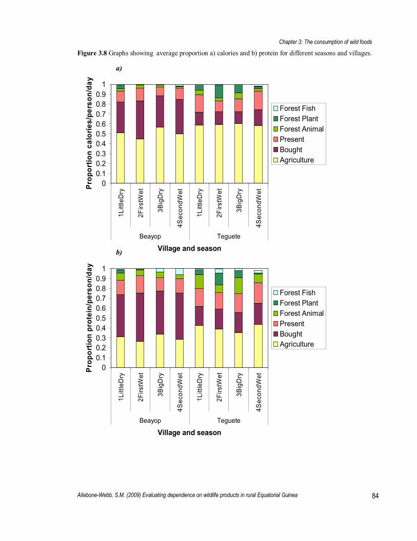
Chapter 3: The consumption of wild foods
Allebone-Webb, S.M. (2009) Evaluating dependence on wildlife products in rural Equatorial Guinea 84
Figure 3.8 Graphs showing average proportion a) calories and b) protein for different seasons and villages.
00.10.20.30.40.50.60.70.80.9
1
1Litt
leD
ry
2Firs
tWet
3Big
Dry
4Sec
ondW
et
1Litt
leD
ry
2Firs
tWet
3Big
Dry
4Sec
ondW
et
Beayop Teguete
Village and season
Prop
ortio
n ca
lorie
s/pe
rson
/day
Forest FishForest PlantForest AnimalPresentBoughtAgriculture
00.10.20.30.40.50.60.70.80.9
1
1Litt
leD
ry
2Firs
tWet
3Big
Dry
4Sec
ondW
et
1Litt
leD
ry
2Firs
tWet
3Big
Dry
4Sec
ondW
et
Beayop Teguete
Village and season
Prop
ortio
n pr
otei
n/pe
rson
/day
Forest FishForest PlantForest AnimalPresentBoughtAgriculture
a)
b)
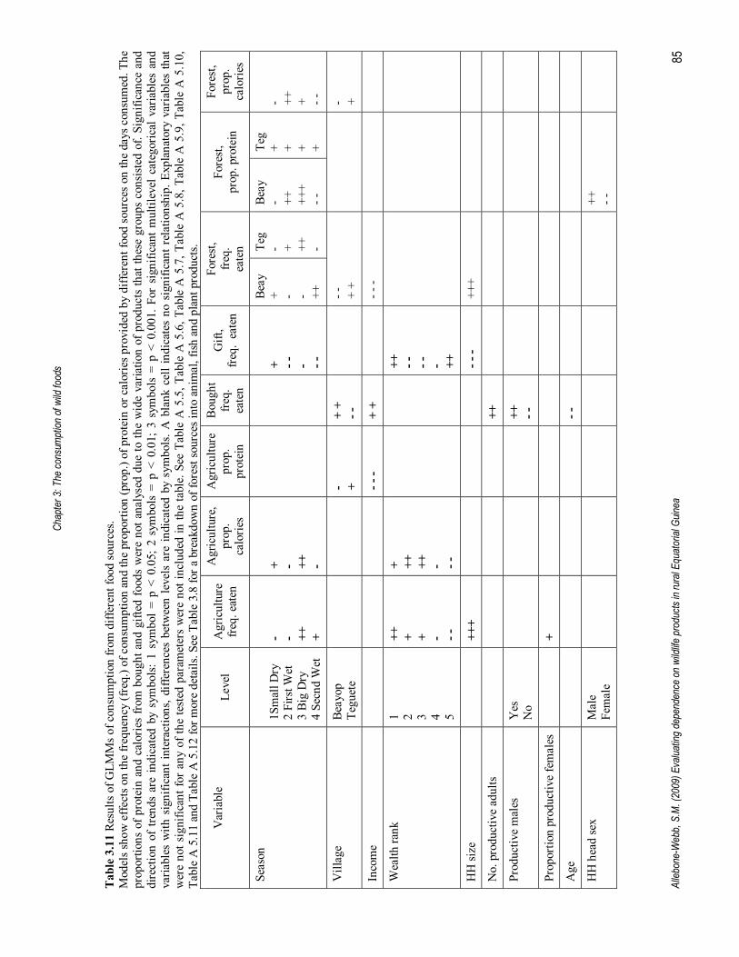
Chap
ter 3
: The
cons
umpt
ion of
wild
food
s
Alleb
one-
Web
b, S
.M. (
2009
) Eva
luatin
g de
pend
ence
on
wildl
ife p
rodu
cts in
rura
l Equ
ator
ial G
uinea
85
Tab
le 3
.11
Resu
lts o
f GLM
Ms o
f con
sum
ptio
n fr
om d
iffer
ent f
ood
sour
ces.
M
odel
s sho
w e
ffect
s on
the
freq
uenc
y (f
req.
) of c
onsu
mpt
ion
and
the
prop
ortio
n (p
rop.
) of p
rote
in o
r cal
orie
s pro
vide
d by
diff
eren
t foo
d so
urce
s on
the
days
con
sum
ed. T
he
prop
ortio
ns o
f pro
tein
and
cal
orie
s fr
om b
ough
t and
gift
ed fo
ods
wer
e no
t ana
lyse
d du
e to
the
wid
e va
riatio
n of
pro
duct
s th
at th
ese
grou
ps c
onsi
sted
of.
Sign
ifica
nce
and
dire
ctio
n of
tre
nds
are
indi
cate
d by
sym
bols
: 1
sym
bol
= p
< 0.
05;
2 sy
mbo
ls =
p <
0.0
1; 3
sym
bols
= p
< 0
.001
. For
sig
nific
ant m
ultil
evel
cat
egor
ical
var
iabl
es a
nd
varia
bles
with
sig
nific
ant i
nter
actio
ns, d
iffer
ence
s be
twee
n le
vels
are
indi
cate
d by
sym
bols
. A b
lank
cel
l ind
icat
es n
o si
gnifi
cant
rel
atio
nshi
p. E
xpla
nato
ry v
aria
bles
that
w
ere
not s
igni
fican
t for
any
of t
he te
sted
par
amet
ers
wer
e no
t inc
lude
d in
the
tabl
e. S
ee T
able
A 5
.5, T
able
A 5
.6, T
able
A 5
.7, T
able
A 5
.8, T
able
A 5
.9, T
able
A 5
.10,
Ta
ble
A 5
.11
and
Tabl
e A
5.1
2 fo
r mor
e de
tails
. See
Tab
le 3
.8 fo
r a b
reak
dow
n of
fore
st so
urce
s int
o an
imal
, fish
and
pla
nt p
rodu
cts.
Var
iabl
e
Leve
l A
gric
ultu
re
freq
. eat
en
Agr
icul
ture
, pr
op.
calo
ries
Agr
icul
ture
pr
op.
prot
ein
Bou
ght
freq
. ea
ten
Gift
, fr
eq.
eate
n
Fore
st,
freq
. ea
ten
Fore
st,
prop
. pro
tein
Fore
st,
prop
. ca
lorie
s
Seas
on
1Sm
all D
ry
2 Fi
rst W
et
3 Bi
g D
ry
4 Se
cnd
Wet
- - ++
+
+ - ++
-
+ - -
- - -
Beay
+ - - ++
Teg
- + ++
-
Beay
- ++
++
+ - -
Teg
+ + + +
- ++
+ - -
Vill
age
Beay
op
Tegu
ete
- + +
+ - -
- -
+ +
- +
Inco
me
- -
- +
+
- - -
Wea
lth ra
nk
1 2 3 4 5
++
+ + - - -
+ ++
++
- - -
++
- -
- -
- ++
HH
size
+++
- -
- ++
+
No.
pro
duct
ive
adul
ts
++
Prod
uctiv
e m
ales
Y
es
No
++
- -
Prop
ortio
n pr
oduc
tive
fem
ales
+
Age
- -
HH
hea
d se
x M
ale
Fem
ale
++
- -

Chap
ter 3
: The
cons
umpt
ion of
wild
food
s
Alleb
one-
Web
b, S
.M. (
2009
) Eva
luatin
g de
pend
ence
on
wildl
ife p
rodu
cts in
rura
l Equ
ator
ial G
uinea
86
Tab
le 3
.12.
Tab
le sh
owin
g re
sults
of G
LMM
s of c
onsu
mpt
ion
from
fore
st fo
od s
ourc
es a
gain
st al
l exp
lana
tory
var
iabl
es.
Mod
els s
how
eff
ects
on
the
freq
uenc
y of
con
sum
ptio
n an
d th
e pr
opor
tion
of p
rote
in p
rovi
ded
by fo
rest
terr
estri
al a
nim
als (
bush
mea
t) an
d fis
h on
the
days
con
sum
ed. P
rote
in
cont
ribut
ion
(as
oppo
sed
to c
alor
ie)
was
ana
lyse
d be
caus
e th
ese
prod
ucts
wer
e m
ore
impo
rtant
for
ove
rall
prot
ein
cons
umpt
ion.
Sig
nific
ance
and
dire
ctio
n of
tren
ds a
re
indi
cate
d by
sym
bols
: 1 s
ymbo
l = p
< 0
.05;
2 s
ymbo
ls =
p <
0.0
1; 3
sym
bols
= p
< 0
.001
. For
sig
nific
ant m
ultil
evel
cat
egor
ical
var
iabl
es a
nd v
aria
bles
with
sig
nific
ant
inte
ract
ions
, diff
eren
ces b
etw
een
leve
ls a
re in
dica
ted
by sy
mbo
ls. A
bla
nk c
ell i
ndic
ates
no
sign
ifica
nt re
latio
nshi
p. E
xpla
nato
ry v
aria
bles
that
wer
e no
t sig
nific
ant f
or a
ny o
f th
e te
sted
par
amet
ers w
ere
not i
nclu
ded
in th
e ta
ble.
See
Tab
le A
5.1
3, T
able
A 5
.14,
Tab
le A
5.1
5, T
able
A 5
.16
and
Tabl
e A
5.1
7 fo
r det
ails.
Var
iabl
e Le
vel
Fore
st a
nim
al,
freq
uenc
y ea
ten
Fore
st a
nim
al,
prop
ortio
n pr
otei
n Fo
rest
fish
, fr
eque
ncy
eate
n Fo
rest
fish
, pr
opor
tion
prot
ein
Fore
st p
lant
, fr
eque
ncy
eate
n
Seas
on
1Sm
all D
ry
2 Fi
rst W
et
3 Bi
g D
ry
4 Se
cond
Wet
++
- -
+ -
Beay
. - ++
+ - +
Teg.
- - ++
- -
- ++
- -
+
- + + ++
Beay
. - - -
- -
- -
Teg.
++
++
+ ++
+ +
Vill
age
Beay
op
Tegu
ete
- -
++
- -
- ++
+
- -
++
Inco
me
++
+
-
Wea
lth ra
nk
1 2 3 4
- ++
+ - -
- ++
+ - -
HH
size
++
++
+
+++
HH
hea
d se
x M
ale
Fem
ale
+++
- - -

Chapter 3: The consumption of wild foods
Allebone-Webb, S.M. (2009) Evaluating dependence on wildlife products in rural Equatorial Guinea 87
3.5 Discussion
This study provides some evidence with which to examine the hypotheses laid out in the
introduction, although not all as expected:
1. More remote communities consume more wild foods
As expected, people in the more remote community of Teguete consumed significantly more wild
foods and gained a significantly higher proportion of macronutrients from them.
2. Inconclusive evidence that wealthier households eat more bushmeat
There was some evidence to support the hypothesis that wealthier households eat more bushmeat.
Wealthier people in both villages ate more protein in general, and the higher wealth ranks in both
villages ate the most bushmeat, both hunted by the household and in general. In addition, middle
wealth ranks ate bushmeat produced by the household more often than poorer or wealthier ranked
households. However, there were no significant relationships between wealth and the frequency or
proportion of bushmeat consumption, and the poorer wealth ranks as well as wealthier ranking
households also gained a high proportion of protein from bushmeat in Teguete. This, and the lack of
discernable differences in wild fish consumption, mean that these results support those found by
Kümpel (2006) and suggest that the increased protein consumption by wealthier households is due
to higher quantities of meat and fish consumption in general, but that this does not particularly
consist of wild meat or fish.
3. No clear relationship between wild plant consumption and wealth
Wild plants were eaten most in Teguete, arguably the poorer village, and there, wild plants were
eaten most often by poorer households, although wealthier households still showed high
consumption of these products. In contrast, wild plants were eaten most often by wealthier
households in Beayop, and I suggest that this disparity is due to the different status and desirability
of various wild plants. Some wild plants, such as forest-harvested leafy greens, could be considered
�food of the poor�, and households may eat these greens when there are no other foods available
(see Chapter 5, and reported by Jamiya (2007) in other countries). Other wild foods are perhaps a
substitute for equivalent or preferred bought products, and this includes palm oil (as opposed to
vegetable oil) and palm wine (as opposed to purchased, imported beer, wine or spirits)5, and so are
5 Palm products were considered a forest food source when they were harvested directly from the forest.

Chapter 3: The consumption of wild foods
Allebone-Webb, S.M. (2009) Evaluating dependence on wildlife products in rural Equatorial Guinea 88
also foods of the poor. A third category of wild plant products are preferred and are widely traded in
other countries. In particular, this includes the bush mango, which is twice the price of peanuts (by
volume) and for which demand is high enough to have provoked domestication programmes in
other countries (Atangana et al. 2002). Bush mango is less widely harvested in Beayop, so may be
consumed more often by wealthier households that can afford to buy it.
4. Poorer households consume more products directly sourced by the household
The second poorest wealth ranks produced ate the greatest proportion of protein and calories
produced by the household. The poorest wealth ranks were often unable to produce much food,
either due to low labour availability in the household (reflected in low proportions of active adults
and recognised as a characteristic of poorer households during the wealth ranking exercise � see
Chapter 2), and so relied on gifts of food more than other households. The exception was for the
poorest households in Beayop, who produced the greatest proportion of protein themselves than
other households in the village, and the results suggest that this is made up of increased protein
from agricultural products, as opposed to animal or fish products. This may be because where
people are more likely to give gifts of food they have produced themselves (rather than bought), in a
village where less bushmeat is hunted (and so less animal protein produced by the village), the gifts
received by the poor are less likely to be meat.
5. Wild foods, particularly plants, contribute more to consumption in the �hungry� season in
Teguete, but not in Beayop
Focus groups identified the second season as the �hungry� season, mainly due to the reduced
agricultural harvest and increased agricultural labour during this period (Chapter 2) and this is
supported by additional evidence in Chapter 5. Households in Teguete consumed the greatest
proportion of calories and protein from wild products in seasons 2 and 3, and overall proportion
consumption from wild plants was particularly high in the second season, when wild plants are
eaten more often. This suggests that wild plants are important for both protein and calorie
consumption during the lean season in rural villages. However, households in Beayop do not show
increased consumption of wild foods during the lean season, and this may be due to reduced access
to forest foods, or increased access to alternative food sources (and livelihoods � see Chapter 4).
3.5.1 Additional observations
Average calorie and protein consumption levels recorded are lower than the daily recommended
amounts. However, this may be the result of consistent under-estimation of food quantities and so it

Chapter 3: The consumption of wild foods
Allebone-Webb, S.M. (2009) Evaluating dependence on wildlife products in rural Equatorial Guinea 89
it is difficult to draw any real conclusions as to whether overall consumption needs are being met,
particularly because activity levels (and so actual energy requirements) have not been reported.
However, any under-reporting is likely to be consistent across groups, and so we can still have
confidence in comparisons between individuals and households.
The results also suggest that households are more able to produce food to meet energy needs than
protein requirements, as reflected in the higher proportion of calories eaten from food produced by
the household, than protein. This difficultly in obtaining protein may be greater in areas with lower
forest offtake, such as Beayop. People in countries such as Equatorial Guinea, where there is a
heavy reliance on carbohydrate staples that are very low in protein (such as cassava) are most likely
to consume inadequate protein, even when energy consumption is sufficient (Svedberg 2000), and
an inability to produce enough protein to fulfil consumption needs affects poor households more
than wealthier households, who are able to purchase food from other sources. These results suggest
that the poorest households in communities with lower access to forests are more at risk from
deficiencies in the diet protein than the poorest households in more rural villages, who can access
forest protein resources.
One major limitation of this study is the inability to detect differences in individual consumption
within households. Evidence shows that intrahousehold allocation of resources, including food, can
vary significantly, particularly between genders and age groups (Haddad et al. 1996). The
communal nature of food consumption in this study, with households commonly sharing food from
an actual shared pot, made it impossible to accurately assess differences in food consumption within
households with the resources available, so I was unable to test these hypotheses.
In conclusion, the data do show that wild foods can play an important role in diets, and this is
particularly true of bushmeat and wild plants, and of more rural communities. Wild plants may be
particularly important during the lean season, and the loss of wild food products in communities
with less forest access is most likely to impact protein and calorie consumption of the poorest
households.
Chapter 4.
The contribution of wildlife
to livelihoods

Chapter 4: The contribution of wildlife to livelihoods
Allebone-Webb, S.M. (2009) Evaluating dependence on wildlife products in rural Equatorial Guinea 91
4.1 Abstract
Recent studies have shown that forest products can be more important for income than for
consumption, and so in this chapter I aim to quantify the production and income from forest
products compared to other income sources. I show that poorer households harvest the most forest
products, and of these, bushmeat is the most important. Income per hunter increases with wealth,
but averaged over all people, bushmeat provides most income to the poor. Poorer households earn
less income from other livelihood activities such as trade and paid work, and may be less able to
compensate during the 2nd and 3rd seasons when agricultural productivity is lowest. Gender
divisions between livelihood activities remain strong, with men generally hunting, and women
cultivating agricultural food staples. The collection of forest plant products is also divided by
gender, with men harvesting more valuable, generally non-edible wild plants, and women
harvesting low value wild plant foods that are not widely traded in Equatorial Guinea.
4.2 Introduction
In the past, harvesting non-timber forest products in tropical regions has often been considered as
primarily a subsistence activity, with all products being consumed in the home. Evidence now
shows that harvesting wildlife can play a key role in the livelihood activities of poor, rural
populations (Pimentel et al. 1997; Mainka & Trivedi 2002) and some have estimated that wildlife
makes up a significant and direct part of the livelihoods of up to 150 million people (Bennett &
Robinson 2000). Forest products can contribute considerable revenue to households (Juste et al.
1995) and indeed, income from wildlife sales can be more important than its value as a food
resource (Godoy et al. 1995; de Merode et al. 2004). Despite this, many forest products do not
appear on countries� balance sheets or development frameworks (Bird & Dickson 2007), and trade
in these products is often not part of the formal economy. As a result, their value for income
generation is consistently underestimated, and the cost to rural households of replacing these
products with bought items even more so (Narendran et al. 2001; Delang 2006). Wildlife can be
important in providing a supplementary income (UNDP 2005), with households gaining 40-60% of
income from NTFPs, and as high as 80% where alternative income sources do not exist. Another
study in Cameroon put income from forest activities at over half of local incomes (Chege 1994).
Of all tropical forest products, bushmeat is thought to be of particular value in many areas. Meat
generally has a higher value per unit weight or volume than other forest products, can be relatively
easily stored and transported, and may be the only source of ready cash in a subsistence economy.

Chapter 4: The contribution of wildlife to livelihoods
Allebone-Webb, S.M. (2009) Evaluating dependence on wildlife products in rural Equatorial Guinea 92
In sub-Saharan African, bushmeat hunting is a common component of household economies
(Asibey 1977; ma Mbalele 1978; Martin 1983; Anadu et al. 1988; Geist 1988; King 1994; Juste et
al. 1995) and in some cases, hunters and traders earn higher than average annual earnings (Dethier
1995; Ngnegueu & Fotso 1996). Even as a supplementary income, hunting was shown to be
essential to farmers in a number of African countries (Bissonette & Krausman 1995) albeit on a
small scale, with farmers hunting during the agricultural low season, when there are lower labour
requirements. In Equatorial Guinea, studies have shown that hunting may be more important for
income than food, and in two hunter villages studied, hunting was both widespread and a major
income source, rivalling salaries for some individuals (Kümpel 2006; Rist 2007). Other studies have
shown bushmeat to be sold and consumed across much of Río Muni (Albrechtsen 2007).
The contribution of wild insects and other invertebrates to income can be significant. In Botswana,
the sale of the caterpillar Imbrasia belina was the third biggest source of income after the sales of
poles and livestock, contributing 13% of total household monetary income (Zitzmann 1999). In
Central Africa, there is a strong trade in insects, with insects being widely available in village
markets, and even some city markets and restaurants (de Foliart 1992). There also appears to be
significant international trade, both within the central African region, and to other countries in
Africa and Europe. Tabuna (2000) reports that 5 and 3 tonnes of dried Imbrasia spp. are imported
annually to France and Belgium respectively from DRC, valued at US$ 41,500 in the case of
Belgium.
Inland wild fisheries are less often studied, but studies have shown that inland water systems can be
particularly important for poorer people at a community and country-wide scale (DFID 2002).
Inland fisheries are often more accessible than marine fisheries; using simple, low-cost
technologies, not requiring regular labour inputs (so they can be fitted around a season�s
agricultural labour requirements) and with the division of labour less strict than for marine fisheries
(where men commonly fish, and women process and trade), meaning that women and children are
more likely to be involved with small-scale inland fishing (DFID 2002). However, it is widely
believed that inland fisheries are greatly underreported (Revenga & Cassar 2002), particularly
because the production of fish for household consumption, and the production of other aquatic
organisms such as crustaceans and molluscs, are not included (FAO 2006). In addition, the
characteristics of inland fisheries � often informally dispersed and with diverse types of fishing
equipment and methods � mean that conventional data collection methods derived from marine
fisheries are less suitable.
Chapter 4: The contribution of wildlife to livelihoods
Allebone-Webb, S.M. (2009) Evaluating dependence on wildlife products in rural Equatorial Guinea 93
In Asia, inland fisheries have been ranked by resource users as the second most important NTFP
(Foppes & Ketphanh 1997) and studies have shown them to be the second biggest earner of income
from NTFPs (Foppes & Dechaineux 2000). Africa has a particularly high rate of per capita inland
fish production amongst its developing countries, and of the global top 10 countries with the highest
inland fisheries capture production per capita, seven are in Africa (in order � Uganda, Tanzania,
Chad, Mali, Gabon, DRC and Zambia, FAO 2006). Although the large lakes present in Uganda,
Tanzania and Chad are predominantly responsible for the high inland fish harvests in these
countries, the importance of inland fisheries in Gabon suggests that it could be important in
neighbouring Equatorial Guinea, but very few data are available. One study by Cogels (1997)
reported that reported that 15% of men fished in certain seasons, and that this provided 42% of the
income in a village situated less than 5km from a broad part of the large river Campo in Equatorial
Guinea. Similarly, Cayuela Serrano et al (2000) show that wild fish accounted for 12% total income
in a village 2km from the river Wele, with 29% of all catch sold, but don�t report any income from
fishing for the other two villages studied. Little else is known about inland fishing in Equatorial
Guinea.
Wild plants have been shown to be important for income, as well as consumption (Delang 2006;
Delang 2006), and may be particularly important for poor and marginalised households and women
(Neumann & Hirsch 2000; Kaimowitz 2003; Shackleton & Shackleton 2006). There are usually
fewer barriers to entry for the harvesting of plant NTFPs than for bushmeat hunting � many people
already have the skills and knowledge to harvest the products, raw products can often be harvested
at little or no cost (except labour), and if there is a market, minimal capital is required to begin
trading. Income from plant NTFPs is often low but can vary considerably, with some producers and
traders gaining income rivalling that of teachers� salaries in west and central Africa (Awono et al.
2002; Ndoye & Awono 2005) and even earning enough to raise their standard of living (Shackleton
2005). Although this may not be enough to lift households out of poverty, income from the local
NTFP trade can have an equalising effect, lowering disparities between households (Fisher 2004).
Some forest plants are even exported from central Africa to Europe (Mialoundama 1993).
Not all studies have shown NTFPs to be important for livelihoods. Ambrose-Oji (2003) found
NTFPs made up at most 6% of income in a forest migrant community in Cameroon, and that it was
the wealthier households that were more likely to earn this. There is little information on the role of
wild plants for livelihoods in Equatorial Guinea, beyond one study showing wild plants for sale in
Bata markets (Sunderland & Obama 1998). However, of the plant NTFP species shown to be of
value in the central African region, some are commonly harvested in Equatorial Guinea. These

Chapter 4: The contribution of wildlife to livelihoods
Allebone-Webb, S.M. (2009) Evaluating dependence on wildlife products in rural Equatorial Guinea 94
include the African plum (Dacryodes edulis) for which commercial production in Cameroon alone
was estimated at US$7.5 million in 1997 (Awono et al. 2002) and is the third most important fruit
crop (after banana and kola). In Cameroon, Bush mango (Irvingia gabonensis) was estimated as
worth US$80-90/year (Ayuk et al. 1999), and there is also a significant trade in Nigeria
(Schreckenberg et al. 2006). Non-food wild plants such as rattan are also important for livelihoods
(Bi & Kouakou 2004), including in Equatorial Guinea (Sunderland et al. 2004).
To determine dependence on forest products we must consider the contribution of wildlife to
income, as well as to consumption. In this chapter, I analyse the income earned and the total value
(including non-sold items) from forest products and to compare this to income and total value
gained from other livelihood activities. Neither study village is specifically a �hunter village� in that
they are not at the end of a road, and are not the closest villages to the forest in the surrounding
area. In addition, both are significantly larger than villages previously studied, are not specifically
visited by traders (although traders do pass through these villages), and Beayop at least is relatively
accessible to urban markets. Consequently, they are more likely to be representative of villages
across Rio Muni than the �specialist� hunting villages previously studied. For these reasons, I
would expect a lower average income from forest products, and bushmeat in particular, in both
Teguete and Beayop, than that seen in previous studies. The greater diversity of livelihood
strategies and trade opportunities afforded by the greater access to urban areas in Beayop means
that I would expect higher incomes in Beayop than Teguete, and for wildlife to make up a lower
proportion of that income.
Previous studies have shown hunting to be predominantly a male occupation (e.g. LeBreton et al.
2006), while women generally dominate the harvest of wild plant foods (Ford Foundation 1998;
Ndoye et al. 1998), although this is not always the case. Studies have shown that households may
vary significantly in the income gained from wild foods according to household wealth. In
Sulawesi, Indonesia, income from wildlife (mainly plants and invertebrates) decreased with wealth
(Pilgrim et al. 2007). De Merode et al (2004) found that income from bushmeat and fish increased
with wealth, but that income from wild plants decreased with wealth in rural households in
Democratic Republic of Congo. A similar pattern was seen in Gabon, where income from bushmeat
increased with wealth, as well as with �remoteness� of a community (Starkey 2004), although
income from hunting as a proportion of total income was highest for medium wealth households.
This has been attributed in part to the fact that wealthier households within these poor rural areas
are often more likely to have healthy, working aged men, and so are more likely to hunt. Given that
the poorest households in this study are likely to lack productive adults (Chapter 2), I would expect

Chapter 4: The contribution of wildlife to livelihoods
Allebone-Webb, S.M. (2009) Evaluating dependence on wildlife products in rural Equatorial Guinea 95
to see a similar result, with medium households gaining more income from bushmeat, at least in
Teguete.
4.3 Methods
Throughout this chapter, I distinguish between the value of production and the income from each
livelihood activity. I take value to be the monetary equivalent of all goods produced or harvested
(regardless of whether they were for sale or consumption) as well as the income or value of any
paid work (i.e. including the value of goods paid in-kind) and the net income from any goods
traded. I take income to be only the cash income from these sources, calculated from what people
have actually sold or earned.
4.3.1 Data Collection
Data were collected on all livelihood activities, including goods produced or harvested, money or
goods earned, and goods traded (including how they were obtained and at what price) in Beayop
and Teguete during regular household interviews with all household members of 18 or over. For
detailed methods and description of the study sites, see Chapter 2.
For forest and agricultural activities, for each sample day the amount (in local units) and value of all
goods produced (including those brought into the house, or consumed or sold before reaching the
house), were recorded as reported by the interviewee. If the respondent could not put a monetary
value on the item, the average value of that item and quantity in that village was used, giving a
monetary value for all goods. Goods that were never sold in either village were not included in the
analyses, and this included water, firewood and the leaves used to wrap cassava. The value of any
forest or agricultural goods actually sold on the sample day (regardless of whether they were
collected on that day) was recorded as actual income. For the two main agricultural harvests, peanut
and calabaza6, the entire crop was often harvested in a matter of days, and so for these products all
households and field owners were questioned at the end of each harvest, and again at the end of the
survey, as to the total number of sacks harvested and sold from each field of these products. Where
possible (and once the crop had had sufficient time to dry), the sacks were weighed and the weights
recorded. The total value of the harvest was estimated using the average price per sack for that
household, or where none had been sold, for that village. The mean value per day for peanuts and
calabaza was taken as the total value of that season�s harvest divided by the number of days of the
6 Calabaza is the local Spanish name for Cucurbitaceae oilseeds (also known as Egusi)

Chapter 4: The contribution of wildlife to livelihoods
Allebone-Webb, S.M. (2009) Evaluating dependence on wildlife products in rural Equatorial Guinea 96
season which it was harvested. Similarly, the mean income per day was taken as the total income
divided by the number of days of the season in which it was sold. Any peanuts or calabaza recorded
in the daily surveys were not included in the calculations, to avoid double counting.
Hunter offtake surveys were done in both villages for the final 7 months of the survey. Each
weekend, from Saturday afternoon to Sunday evening when all hunters had usually returned to the
village, I and/or a trained research assistant visited all hunters in the village, and asked questions on
all hunting trips for that week. Data were collected on all hunting trips and carcasses captured for
that week, including on which days they had been hunting, the time leaving and returning to the
village, what methods were used on the trip (i.e. trapping, gun, dogs, or a combination of these), and
details of any animals caught, what they did with it (i.e. consumed at home, consumed in the forest,
sold, gave to someone, abandoned in the forest), and if sold, how much for and who to.
For traded goods, the actual income was recorded as being the price it was sold for, minus the
production costs and the initial cost of the item where appropriate. In some cases it was necessary to
estimate the production costs, and where necessary, a case study was done of the activity in
question. For example, this included a calculation of the cost of cooking doughnuts, where women
in each village were observed cooking the doughnuts, with the amount and cost of each ingredient
observed, and the number of doughnuts produced counted, to give an estimated production cost per
doughnut, from which net income could be calculated. In the case of village shops and bars, on
survey days shop owners were asked how much total money they had taken that day. Every two
months, an inventory of each village shop was made, to record the prices of all goods for sale, and
count the amount of stock. Where possible, when bars were restocked, we recorded the amounts of
each good bought, where it was bought from, how much it cost and the estimated travel costs. This
allowed calculation of the mean mark-up on each product for each bar. The weighted average mark-
up for each village shop was calculated using the proportion of goods bought to restock each bar.
Thus, the average mark-up for each bar was calculated, permitting estimation of the net profit given
the total money taken for each survey day.
Respondents with jobs and salaries were initially asked what their monthly salary was, and after that
were only asked in the regular questionnaire if they had received any bonuses in the previous two
weeks. The salary amounts were verified at the end of the study, and any changes made
accordingly. The one respondent who was uncomfortable with answering this question was instead
asked to point to a category on a piece of paper, and the middle value of this range was taken as an

Chapter 4: The contribution of wildlife to livelihoods
Allebone-Webb, S.M. (2009) Evaluating dependence on wildlife products in rural Equatorial Guinea 97
estimate of his income. Details of any casual work were recorded; including type of work, amount
earned, and number of days worked where possible.
To ascertain the differences in livelihood activities between individuals and households, data were
also collected and calculated on household characteristics including household (HH) income, HH
fixed wealth, wealth rank, HH size, number of productive adults (age 18-65 and not chronically ill),
number of productive females, the presence/absence of productive males, proportion of productive
adults (to whole HH size), proportion of productive females, gender of the household head and
education level of the household head. In addition, data on individual age, sex and education levels
were collected, and village and season recorded. See Chapter 2 for methods and details.
4.3.2 Data Analysis
Summary of different income sources
For each livelihood activity, the characteristics of people engaging in that activity (i.e. recorded as
producing anything from that activity) were detailed, including the number of males and females in
each village, the age range, average age, average value/day, average income/day, average
value/year, range of income, average hours/day, average days/week, assets required (e.g.
equipment, land, skills, etc.) and the cost of those assets. For all livelihood activities except hunting,
these data were taken from the regular household surveys. Where appropriate, the major value and
income sources within each category were listed. For hunting, these data were taken from hunter
surveys, as these had a greater number of sample days. Where people engaged in more than one
livelihood activity, they were included in the analysis for all activities in which they participated.
This excluded people who were participating in an activity that they did not usually do (i.e. children
helping in their parents� fields were not included). For trade, where one person bought, produced or
processed a good (e.g. harvested and then cooked bars of cassava) but another person physically
sold it, this income was attributed to the owner of the good � the person who kept the money. This
commonly applied to older children selling goods at the side of the road that had been grown or
processed by adult family members. In these cases, the interviewee was asked both who physically
sold the good, and who earned the money.
The determinants of income and potential income from different sources
Livelihood activities were split into four categories:
• Forest: Any activity harvesting goods non-cultivated products from the forest, farm-fallow
or agricultural land. This was further broken down into the harvesting of animal, fish and

Chapter 4: The contribution of wildlife to livelihoods
Allebone-Webb, S.M. (2009) Evaluating dependence on wildlife products in rural Equatorial Guinea 98
plant products and includes goods that require further processing in the village (i.e. the
production of artisanal products made from rattan, or palm oil harvested from the forest) or
in the forest (i.e. the production of palm wine).
• Agriculture: Activities associated with the production of all agricultural goods and
livestock. Again, this includes goods requiring processing in the village such as the
production of bars of cassava, sales of banana doughnuts, and production of palm oil (if that
oil has been harvested from the fields).
• Trade: Any activity involving the buying and subsequent selling of goods. This was further
divided into goods that were sold with no processing/value added (i.e. the majority of bar
products), and goods that were resold after processing (e.g. doughnuts and bread made in
the village with purchased wheat flour, and meat and fish that had been bought from hunters
and fishers in the village and cooked to sell in single portions along the side of the road).
• Paid: Any activity where the person was paid for their work by another person. This
included salaried work and casual work such as carpentry and payments for clearing fields).
As virtually no domestic animals were recorded as sold during the entire survey, these were not
included in the analyses (except for calculating total household income). For products that were
both cultivated and harvested from the forest (e.g. African plums, oil palms, avocados) the produce
was counted as agricultural if the tree was �owned� by a particular household or growing in a field.
Goods were counted as forest offtake if grown in the forest.
The average daily value and daily income per person per season for each livelihood activity type
was calculated for all people over 18 by taking the average value and income from all sample days
that a person had been interviewed within each season.
Factors affecting who engages in each type of livelihood activity
For each person in each season, whether or not they had harvested �forest� products (i.e. wild
products) was recorded as a binomial variable. This was used to assess the factors affecting who in
each community engaged in �forest� category livelihood activities according to individual and
household characteristics, village and season (see list above) using a generalised linear mixed model
(GLMM) using the lme4 library (Bates & Sarkar 2007):

Chapter 4: The contribution of wildlife to livelihoods
Allebone-Webb, S.M. (2009) Evaluating dependence on wildlife products in rural Equatorial Guinea 99
• Whether or not a person produced �forest� products ~ Village + HH Income + Season + Sex +
(1|Village/HH/Individual), offset = AME) 7
Individual nested within household nested within village were specified as random effects.
Explanatory variables were transformed to give normal distributions where appropriate. Analyses
were done in the same way to assess the factors affecting who gains income from forest products,
and this was repeated for each category of livelihood activity (forest, agriculture, trade and paid
activities) using the following dependent variables: • Whether or not a person gained income from �forest� products
• Whether or not a person produced �agricultural� products
• Whether or not a person gained income from �agricultural�
• Whether or not a person gained income from �trade�
• Whether or not a person gained income from �paid� work
All people who traded or had paid worked gained monetary income, so value produced was the
same as income:
Further analyses were done in the same way to assess the factors affecting wither or not individuals
harvested different types of forest8 products (animal, fish and plant) using the following dependent
variables:
• Whether or not a person produced �forest animal� products
• Whether or not a person produced �forest fish� products
• Whether or not a person produced �forest plant� products
• Whether or not a person gained income from �forest animal� products
• Whether or not a person gained income from �forest fish� products
• Whether or not a person gained income from �forest plant� products
Factors affecting amount of value and income gained for each type of livelihood activity among
resource users
To assess the variations in the value of forest products produced, a further analysis was done using
only data for people who had harvested forest products (i.e. the resource users or �producers�). The
7 For simplicity, not all explanatory variables are shown in these equations. For a full list, see text and section
2.3.1. 8 As specified above, �forest� products refers to all non-cultivated products harvested from the forest, farm-
fallow or agricultural land.

Chapter 4: The contribution of wildlife to livelihoods
Allebone-Webb, S.M. (2009) Evaluating dependence on wildlife products in rural Equatorial Guinea 100
log of the average daily value gained from forest products per person per season was analysed using
a linear mixed model (LMM) in the lme4 library (Bates & Sarkar 2007) to assess variations in the
value of forest products harvested, with explanatory variables as above. Again, individual nested
within household within village were specified as random effects and explanatory variables
transformed where necessary:
• Value of �forest� products harvested ~ Village + HH Income + Season + Sex + (1|Village/HH/Individual)) 9
The analyses were repeated in the same way for income from forest products, for each type of
livelihood activity, and for individual forest products using the following dependent variables:
• Income from �forest� products
• Value of �agricultural� products harvested
• Income from �agricultural� products
• Income from �trade�
• Income from �paid� work
• Value of �forest animal� products harvested
• Value of �forest fish� products harvested
• Value of �forest plant� products harvested
• Income from �forest animal� products
• Income from �forest fish� products
• Income from �forest plant� products
It was not possible to analyse the amount of income earned by all people for an activity, as for any
given activity a large number of people would have gained no income or value, creating many �true-
zeros� in the data set (Martin et al. 2005). This
All data were analysed in R, version 2.6.2 (R Development Core Team 2007). Models were
simplified to obtain the minimum adequate model by fitting the saturated model and then
comparing models with progressively simplified fixed effects using change in deviance tests.
Significance was taken as p<0.05.
9 For simplicity, not all explanatory variables are shown in this equations. For a full list, see text and section
2.3.1.

Chapter 4: The contribution of wildlife to livelihoods
Allebone-Webb, S.M. (2009) Evaluating dependence on wildlife products in rural Equatorial Guinea 101
4.4 Results
4.4.1 General characteristics of livelihoods
Agriculture
Virtually all households maintained at least one field a year of mixed crops (see Table 4.1 for all
details). Fields are planted with peanuts or calabaza and then intercropped with staples such as
cassava, plantains, bananas and sugar cane, with the proportions of each crop varying between field,
household and village. Also cultivated are (in no particular order): leafy greens, maize, onion,
tomatoes, yam, cocoyam, wild peppers and sweet potatoes. Many households also have patches of
cultivated land near the house, where papayas, some leafy greens, bread fruit, chilli peppers and
coconut may be grown. African plums (Dacryodes edulis) and palm fruits were also harvested, and
this was counted as agricultural produce where the trees were owned by a particular household. This
commonly occurred for trees growing close to the village (particularly for African plums) or trees
growing within households� fields (particularly for oil palms, where in land being cleared for
planting, the tree would be left to remain in the field).
With the exception of two men in Teguete, both of whom were over 60 and lived by themselves, no
men had mixed crop fields or grew these dietary staples. Instead, they usually helped clear new
fields, leaving women to cultivate the land for the rest of the year. Some men did help out in their
wives� or mother�s fields, particularly during times of heavy work, or if the female in question was
heavily pregnant or had a small child. However, this was very infrequent, and more often it was
female relatives or friends who would offer support to women temporarily unable to cultivate their
fields. Where men had fields, they were generally semi-permanent fields including trees such as
mangoes, oranges, avocados, African plums or oil palms, with established pineapple plants growing
in between, and consequently did not require as much labour (and certainly not planting or
clearing).

Chapter 4: The contribution of wildlife to livelihoods
Allebone-Webb, S.M. (2009) Evaluating dependence on wildlife products in rural Equatorial Guinea 102
Table 4.1 General characteristics of agriculture
Beayop Teguete Female Male Female Male
Field owner (no. people) 74 2 86 3 Field owner, age range 20 - 80 46 � 65 19 � 82 61 � 92 Field owner, average age 44 56 53 69 Average value/day (cfa) 704 315 356 185 Average income/day (cfa) 805 77 354 117 Average value/year (field owners only) (cfa)
109,925 35,000 60,697 21,667
Average income/year (field owners) (cfa) 21,771 2,500 11,705 9,167 Labour required: Physical intensity of work Clearing fields is particularly labour-intensive, and usually done by
men. However, despite the fact that some women continue to have fields into their 70s and even 80s, all the field work requires physical strength. This is particularly true given that all work is done by hand with a machete (i.e. no mechanisation at all) and because all harvests are carried by basket whose weight is support on the forehead (via a strap) and the back.
Assets required: Property/land Land (see Box 4.1) Equipment: Machete
File (to sharpen machete) 2500 cfa (replaced every 6 months) 1000 cfa (replaced every 3 months)
Other start-up costs Clearing land:
Seeds or tubers to plant (these are usually saved from previous fields to plant in new fields. They are rarely bought, and most people borrow or receive them as gifts). Male family members often clear the land for burning for a new field using an axe or chain saw (if available), but more commonly using a machete. If a woman doesn�t have anyone she can call on to do this, she may pay someone instead (12,000 � 25,000cfa per field).
Social resources For land rights As buffer during illness/pregnancy To help with field clearing
Natural resources Variation in soil quality Differences in climate and the quantity of crop pests (greater in Teguete) meant that Calabaza was grown on a greater scale in Teguete, and sugar cane on a greater scale in Beayop. Peanuts planted in both.
Skills/knowledge education Without ever being formally taught, most women and some men learn agricultural skills, usually from older female (often mothers-in-law) relatives as they help out in the fields as adolescents, or when first married.
Seasonality: Peanuts are mainly harvested in the 1st and 3rd seasons. Calabaza is harvested in the 4th season.
Barriers to entry: A large amount of time needed, physically demanding, and either money or social capital necessary to start-up (to get help clearing fields, and �borrow� or buy seeds and tubers to plant).
Crops giving greatest total value (in order)
Peanuts, cassava, sugar cane (made into Malamba), plantain, calabaza
Cassava, peanuts, calabaza, banana, pineapple
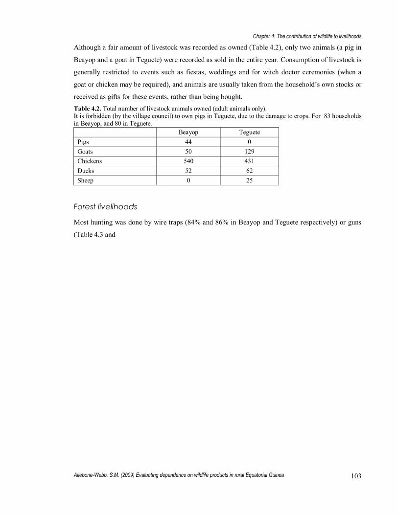
Chapter 4: The contribution of wildlife to livelihoods
Allebone-Webb, S.M. (2009) Evaluating dependence on wildlife products in rural Equatorial Guinea 103
Although a fair amount of livestock was recorded as owned (Table 4.2), only two animals (a pig in
Beayop and a goat in Teguete) were recorded as sold in the entire year. Consumption of livestock is
generally restricted to events such as fiestas, weddings and for witch doctor ceremonies (when a
goat or chicken may be required), and animals are usually taken from the household�s own stocks or
received as gifts for these events, rather than being bought. Table 4.2. Total number of livestock animals owned (adult animals only). It is forbidden (by the village council) to own pigs in Teguete, due to the damage to crops. For 83 households in Beayop, and 80 in Teguete.
Beayop Teguete Pigs 44 0 Goats 50 129 Chickens 540 431 Ducks 52 62 Sheep 0 25
Forest livelihoods
Most hunting was done by wire traps (84% and 86% in Beayop and Teguete respectively) or guns
(Table 4.3 and
Chapter 4: The contribution of wildlife to livelihoods
Allebone-Webb, S.M. (2009) Evaluating dependence on wildlife products in rural Equatorial Guinea 104
Table 4.4). In addition, one male in each village went hunting with dogs, but neither caught
anything, and both abandoned it as being unprofitable. Of the women with traps, without exception
all were traps around their fields and were checked most days when working in those fields. All of
these had initially been set by a male family member, but (especially if that male was no longer in
the village) the female responsible would re-set the traps when necessary, and consume or sell any
animals that were caught.
Fishing was not done as a main livelihood activity by any households, and was mainly a
supplementary activity. Hunters sleeping in the forest commonly took a line and hooks with them,
and would fish for food to consume while in the forest. Some female-headed households and older
households had a fish trap that they would check every morning and these mainly caught small
freshwater crabs and small fish. Young boys sometimes went fishing with a hook and line (although
were often unsuccessful) and in the long dry season (the 3rd season), women sometimes collected a
local plant (�esia�) and used it to poison fish in certain portions of the river, while the water level
was low. Only in Beayop did two men commonly fish and sell their catch, but even this was
secondary to trading in terms of income and value produced.
The most important wild edible plants in terms of income were (in order): bush mango, palm oil,
palm wine, avocado, forest fruit �nsuin� and African plum. These were mainly collected by women,
with the exception of palm wine which was collected by men. Men commonly harvested non-edible
forest plants, and the most important of these were (in order): rattan, palm fronds (for making into
roofs), bamboo, other larger vines (for making baskets) and smaller vines (for tying rattan and
larger vines). In both villages, rattan and other vines were mainly used by older men to make bowls,
baskets and fish traps, that were time consuming to make and sold for a small amounts of money
(i.e. the average bowl cost 300 cfa, and the average basket 2000 cfa). Bamboo was used to make
cheap beds such as those in every kitchen that were often the only seating available, and were
usually made by members of the household as a house was constructed. In Beayop only, two
brothers regularly harvested rattan, and used this to make furniture such as chairs and coffee tables
that they sold in Bata. However, they reported having to walk further into the forest to harvest the
rattan than had previously been necessary, and were not keen on others in the village following suit. Table 4.3. General characteristics of gun-hunting.
Beayop Teguete
Female Male Female Male

Chapter 4: The contribution of wildlife to livelihoods
Allebone-Webb, S.M. (2009) Evaluating dependence on wildlife products in rural Equatorial Guinea 105
No. gun-hunters (including those borrowing other peoples guns)
0 8 10 0 14
Age range (all people gun-hunting) NA 20 � 55 NA 19 � 75
Peop
le
Average age (all people gun-hunting) NA 34 NA 35
Average value/trip (cfa) NA 4660 NA 6417
Range value/trip (cfa) NA 0 � 9000 NA 0 � 62667
Average income/trip (cfa) NA 4100 NA 4596
Range income/trip (cfa) NA 0 - 9000 NA 0 � 47000
Average value/trip, gun & traps (cfa) 11 NA NA NA 4440
Range value/trip, gun & traps (cfa) 3 NA NA NA 0 � 19500
Average income/trip, gun & traps (cfa) 3 NA NA NA 3031
Range income/trip, gun & traps (cfa) 3 NA NA NA 0 � 19500
Prof
itabi
lity
Average annual income, gun (cfa) NA 490,360 NA 360,878
Physical intensity of work Medium
Average hours per day NA 4.0 NA 7.57
Average days/week NA 2.3 NA 1.51
Night hunting (No. people) 0 2 0 1 12
Labo
ur re
quire
d
Night hunting (av. No hours) NA 8.9 NA 5
Equipment Gun: No. of owners
No. households with a gun Average cost per gun (cfa)
5 4 156,666
8 4 148,000
600
Cos
ts
Other running costs Average cost per cartridge (cfa)
Torch and batteries (night-hunting only) Gun hire
Some hunters borrow guns from others in the village, and usually pay them back with a portion of their catch rather than money
Social resources No formal permission required, but see Box 4.1.
Res
ourc
es
Natural resources Forest and wildlife
10 Three 12 year old boys also took out a gun one time to practice, but they didn�t catch anything, and are not
included in these calculations 11 In Teguete, some hunters took their guns with them when they checked their traps, and the average value
and income for these combined trips are shown here. 12 The one hunter in Teguete that went night hunting, went only once, whereas the two in Beayop were
regular night hunters

Chapter 4: The contribution of wildlife to livelihoods
Allebone-Webb, S.M. (2009) Evaluating dependence on wildlife products in rural Equatorial Guinea 106
Skills/knowledge education It does take skill and practice to be a good shot, and (particularly given the cost of guns and cartridges), this is something that many people don�t have. Skills tend to be passed on within males of the same family, and for that reason the guns and gun-hunters are relatively concentrated within a few households in each village.
Barriers to entry: Limited access to skills and high start up costs (gun)

Chapter 4: The contribution of wildlife to livelihoods
Allebone-Webb, S.M. (2009) Evaluating dependence on wildlife products in rural Equatorial Guinea 107
Table 4.4. General characteristics of trapping. Beayop Teguete
Female Male Female Male
No. people (having traps) 4 37 2 83
Age range 18 � 50 11 � 90 40 � 57 11 � 92
Peop
le
Average age 35 39 49 42
Average value/trip (cfa) 667 1445 48 1477
Range value/trip (cfa) 0 - 5500 0 � 18000 0 - 921 0 � 25323
Average income/trip (cfa) 304 782 7 696
Range income/trip (cfa) 0 - 5500 0 � 18000 0 - 400 0 � 25000
Prof
itabi
lity
Average annual income (cfa) 37,939 109,793 1,929 72,384
Physical intensity of work Medium
Average hours per day 0.7 5.2 0.8 7.4
Average days/week 2.4 2.7 5.3 2.0
Sleeping away from the village (no. people)
0 0 0 13
Labo
ur
Sleeping away from the village (av. no. nights)
NA NA NA 2.9
Equipment Wire (average cost, cfa)
200/m
275/m
Other start-up costs None
Cos
ts
Other running costs None
Social resources No formal access or permission is required, but see Box 4.1.
Natural resources Forest and wildlife
Res
ourc
es
Skills/knowledge education It does take skill and practice to set traps successfully, but most boys learn to do this to some degree, usually from older male family members.
Trade
In each village there were a number of small shops/bars, and these were where most trade was done.
In addition, items such as cassava bars, local doughnuts, meat and fish (cooked and sold with
cassava), bread and fruits were commonly sold on the side of the road.
Paid work
In Teguete, the only jobs with salaries were those of the four teachers and the one health centre
worker. In Beayop, in addition to the teachers and health centre worker, a few men had paid jobs
with a road building company, but the company soon moved, and the men moved with it. There was
also one bar/restaurant large enough to employ someone full time. Aside from salaried jobs, the

Chapter 4: The contribution of wildlife to livelihoods
Allebone-Webb, S.M. (2009) Evaluating dependence on wildlife products in rural Equatorial Guinea 108
only paid work was mainly done by the one or two carpenters in each village (sometimes employed
to build people�s houses), or by men paid by (often female headed) households to clear fields.
Despite a national minimum wage of 90,000 cfa/month, teachers and health centre workers reported
wages of 75,000 � 120,000 per month, while the one man working in the bar earned
50,000cfa/month. Box 4.1. Access to land Agriculture
Access to land is relatively informal, but varies between the two villages. In Beayop (a more densely
populated area), land around the village is divided among the households according to historical use of
particular areas. These unmarked boundaries remain even during the fields� fallow periods, and generally a
household�s plots of land are relatively close to their own house. As the village has expanded, existing
households have moved further away from the village and cleared new patches of forest to create more land
that is officially theirs. This is limited by strict boundaries between villages, so that villagers in Beayop
cannot create a field in new land that �belongs� to neighbouring villages. However, the village is bounded
only on three sides, while on the fourth side there are no villages for a considerable distance, so boundaries
here are less strictly upheld, if at all. In practice, virtually no mature forest has been cleared in the last
decade, as almost all the land in the area surrounding the village is secondary forest, having been converted
to plantations during the colonial period13. New families moving to the village may take over land of family
members in the village, or may appeal to the village council. The village council will then discuss the matter
and generally can resolve it by asking other families who have more land than they can cultivate (including
fallow land) to let the new family use that land. There are very few disputes, but those arising are resolved by
the village council � a group of elders (mainly men) who discuss the issue. However, the people in Beayop
are aware that land can be an issue, and count themselves lucky that they still have enough. Many know
friends of relatives in village closer to Ebibeyin, where there are more conflicts over land, due to a much
higher population density. In Teguete, the situation is fairly similar, except that the boundaries are less well
known, and neighbouring villages are far enough away that there are no official limits between villages.
Hunting
As for agriculture, there are clearer restrictions on hunting in Beayop than in Teguete, with the same village
boundaries existing for hunting as for agriculture. However, these boundaries are less enforceable for
hunting, and while a trapper may sabotage the traps of someone he doesn�t recognise (or doesn�t know who
they belong to), a trapper is unlikely to chance upon many foreign traps without concerted effort. Enforcing
land boundaries on gun-hunters is virtually impossible, unless the hunter enters the forest from the village
(which is highly unlikely). Between households, there are virtually no limitations, although particularly close
13 Equatorial Guinea is unusual in that land covered by forest has actually increased in the last 30 years, as
land converted to plantations returned to secondary forest.
Chapter 4: The contribution of wildlife to livelihoods
Allebone-Webb, S.M. (2009) Evaluating dependence on wildlife products in rural Equatorial Guinea 109
to the village hunters tend to know along which paths other people�s traps are, and will avoid them to find
un-trapped pathways.
Teguete is closer to uninhabited parts of the forest, and consequently there are no boundaries between
villages. Men from other villages pass through the village to go trapping, and there are some pathways
leading off the road some way away from the village that are commonly known to be trapped by people from
particular villages. However, these are loose associations, rather than strict rules, and people say that there
are no problems between villagers or households over hunting land. Between households within Teguete,
very few people know where the traps of another person are, beyond a general direction, and this information
is guarded quite strongly. The exception to this is that pairs or groups of three men may trap together, and
they will know the whereabouts of the other group members� traps (and may check them for each other if one
is ill or unavailable). Gun hunters from the village and surrounding villages are similarly not restricted in
access, but the very infrequent (maybe one a year) �leisure� gun hunters from the city have been known to be
charged by the village president. Soldiers from the military post inside the village or elsewhere are not
charged, and some have shot a considerable number of animals. However, these were not monitored, and
varied with the individuals involved (who rotated every three months).
4.4.2 Determinants of production and income
Overall production/income
Production and income from all sources combined was higher in Beayop (Table 4.5 and Figure 4.2,
Table A 6.1). In both villages, production and likelihood of income per household were lowest in
season 2, while income varied differently between seasons, depending village (Table A 6.1 and
Table A 6.2). In addition, male-headed households, and households with a higher proportion of
productive females produced more per AME per household, and men in general produced more and
earned higher incomes than women (Figure 4.2).
Community differences in production and income
Across all people, forest products combined provided over half of total livelihood production in
Teguete and nearly a quarter in Beayop, including 25% and 12% from bushmeat (Table 4.5). People
harvesting forest products produced more in general, and specifically more wild plants per season,
and people in Teguete were significantly more likely to get income from forest products as a whole
(Table 4.7 , Table 4.8), and bushmeat specifically (Table 4.9). In contrast, people in Beayop gained
nearly twice the production and three times the income from agriculture across the whole village,

Chapter 4: The contribution of wildlife to livelihoods
Allebone-Webb, S.M. (2009) Evaluating dependence on wildlife products in rural Equatorial Guinea 110
and this accounted for a greater proportion of production and income (Table 4.5). Amongst people
that sold agricultural products, average income per day was also significantly higher in Beayop
(Table 4.10). There were no significant differences in income from trade between villages (
Table 4.11), but people in Beayop did earn substantially more from processed traded goods (Table
4.5).
With only five or six regularly employed people in each village, no analyses were done on the
determinants of paid work. However, with the exception of the man working at the restaurant in
Beayop, all wage earners in both villages had higher education and qualifications for their jobs, and
were mainly men (one or two female teachers were employed in each village, but were nursery or
infant school teachers with lower salaries). Similarly, very little fish was recorded harvested or sold
in either village, and because of this no statistically significant differences in fish harvests or sales
were found.
Trade contributed the greatest total amount of income in Beayop � significantly more than in
Teguete. In particular, people in Beayop earned more from value-added products sold at the side of
the road, while income from products with no value-added (e.g. most bar products) was only
slightly less in Teguete (Figure 4.1). Table 4.5 Summary average production values and income per person for livelihood types in both villages. Mean value produced/day for the whole village is the mean value per person of all goods from each livelihood
type, for all people (including those not producing that good). Similarly for mean income/day.
Mean value produced/day (cfa),
whole village
Mean income/day (cfa),
whole village
Percentage production,
whole village
Percentage income, whole village Livelihood
type Beayop Teguete Beayop Teguete Beayop Teguete Beayop Teguete
Agriculture 269.0 138.2 101.0 29.1 39.6% 27.7% 24.6% 15.0%
Paid Salary 91.7 42.4 91.7 42.4 13.5% 8.5% 22.4% 21.8%
Paid Casual 13.6 5.9 13.6 5.9 2.0% 1.2% 3.3% 3.1%
Trade VA 84.2 6.0 84.2 6.0 12.4% 1.2% 20.5% 3.1%
Trade VNA 63.4 37.5 63.4 37.5 9.3% 7.5% 15.5% 19.3%
Forest (all) 157.3 269.7 56.3 73.3 24.5% 57.6% 13.7% 39.4%
Forest animal 79.3 126.7 29.1 65.1 11.7% 25.4% 7.1% 33.5%
Forest fish 37.1 21.8 15.5 0.2 5.5% 4.4% 3.8% 0.1%
Forest plant 40.9 121.2 11.7 7.9 6.0% 24.3% 2.8% 4.1%

Chapter 4: The contribution of wildlife to livelihoods
Allebone-Webb, S.M. (2009) Evaluating dependence on wildlife products in rural Equatorial Guinea 111
Table 4.6 Percentage of production sold (of the total value produced), and mean income per day (earners only) for livelihood types in each village.
Mean percentage of production sold,
whole village
Mean income/day (cfa), earners only Livelihood
Type Beayop Teguete Beayop Teguete
Agriculture 37.53% 21.1% 943.36 358.51
Paid Salary NA NA 1370.31 1511.74
Paid Casual NA NA 580.79 235.78
Trade VA NA NA 1094.10 266.76
Trade VNA NA NA 758.18 405.67
Forest (all) 33.83% 26.6% 841.32 666.57
Forest animal 36.72% 51.4% 725.69 930.04
Forest fish 41.75% 1.06% 1158.33 83.33
Forest plant 28.50% 6.54% 686.94 202.13
Household and individual differences in livelihoods
Across wealth groups as a whole, forest products provided the most value and income to the poorest
wealth ranks (Figure 4.1), although it was more important to the poorest wealth rank for production
in Beayop, and for income in Teguete. Within individuals harvesting forest products, those from
poorer households harvested significantly more per day on average, although wealthier households
harvested the second highest amounts (

Chapter 4: The contribution of wildlife to livelihoods
Allebone-Webb, S.M. (2009) Evaluating dependence on wildlife products in rural Equatorial Guinea 112
Table 4.7). In contrast, among bushmeat hunters, those from wealthier households gained the
highest amount and income per day (Table 4.9). People in the poorest wealth ranks were most likely
to gain income from bushmeat sales, but within these ranks, wealthier people were more likely to
sell bushmeat (Table 4.9).
The middle wealth ranks were significantly more likely to sell agricultural products, and in Beayop
produced and sold most across the group (Figure 4.1 and Table 4.10). Wealthier households on
average gained more from trade than poorer households, were more likely to trade, and wealthier
traders gained significantly more income per trader (
Table 4.11). People in households where the household head had a higher level of education were
significantly more likely to trade, as were people from female-headed households (Table 4.11).
People with salaries were overwhelmingly in wealthier households (Figure 4.1).
Figure 4.1 The value and income from all livelihood sources, for wealth ranks and villages.
0100200300400500600700800900
1000
1 2 3 4 1 2 3 4 1 2 3 4 1 2 3 4
Value Income Value Income
Beayop Teguete
Village and wealth rank (1 = poorest)
Ave
rage
cfa
/per
son/
day
(all
peop
le)
Trade VNATrade VAPaid CasualPaid SalaryAgricultureForest PlantForest FishForest Animal

Chapter 4: The contribution of wildlife to livelihoods
Allebone-Webb, S.M. (2009) Evaluating dependence on wildlife products in rural Equatorial Guinea 113
0
500
1000
1500
2000
2500
3000
3500
4000
4500
1 2 3 4 1 2 3 4 1 2 3 4 1 2 3 4
Value Income Value Income
Beayop Teguete
Village and wealth rank (1 = poorest)
Ave
rage
pro
duct
ion
and
inco
me
per H
H p
er d
ay
(cfa
)GiftTrade VNATrade VAPaid CasualPaid SalaryAgriculture.Wild PlantWild FishWild Animal
In both villages, men produced and sold more forest products as a whole (Figure 4.2) and the
majority of this was bushmeat. Men were significantly more likely to hunt and sell bushmeat than
women, and produced more when they did ( Table 4.8 and Table 4.9). However, women harvested
all forest products significantly more often than men and in Teguete produced more when they did (
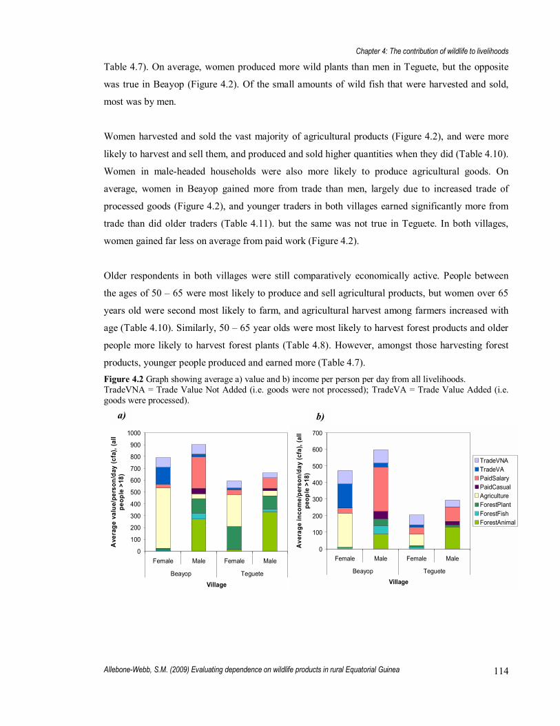
Chapter 4: The contribution of wildlife to livelihoods
Allebone-Webb, S.M. (2009) Evaluating dependence on wildlife products in rural Equatorial Guinea 114
Table 4.7). On average, women produced more wild plants than men in Teguete, but the opposite
was true in Beayop (Figure 4.2). Of the small amounts of wild fish that were harvested and sold,
most was by men.
Women harvested and sold the vast majority of agricultural products (Figure 4.2), and were more
likely to harvest and sell them, and produced and sold higher quantities when they did (Table 4.10).
Women in male-headed households were also more likely to produce agricultural goods. On
average, women in Beayop gained more from trade than men, largely due to increased trade of
processed goods (Figure 4.2), and younger traders in both villages earned significantly more from
trade than did older traders (Table 4.11). but the same was not true in Teguete. In both villages,
women gained far less on average from paid work (Figure 4.2).
Older respondents in both villages were still comparatively economically active. People between
the ages of 50 � 65 were most likely to produce and sell agricultural products, but women over 65
years old were second most likely to farm, and agricultural harvest among farmers increased with
age (Table 4.10). Similarly, 50 � 65 year olds were most likely to harvest forest products and older
people more likely to harvest forest plants (Table 4.8). However, amongst those harvesting forest
products, younger people produced and earned more (Table 4.7). Figure 4.2 Graph showing average a) value and b) income per person per day from all livelihoods. TradeVNA = Trade Value Not Added (i.e. goods were not processed); TradeVA = Trade Value Added (i.e. goods were processed).
0
100
200
300
400
500
600
700
800
900
1000
Female Male Female Male
Beayop Teguete
Village
Ave
rage
val
ue/p
erso
n/da
y (c
fa),
(all
peop
le >
18)
TradeVNATradeVAPaidSalaryPaidCasualAgricultureForestPlantForestFishForestAnimal
0
100
200
300
400
500
600
700
Female Male Female Male
Beayop TegueteVillage
Ave
rage
inco
me/
pers
on/d
ay (c
fa),
(all
peop
le >
18)
TradeVNATradeVAPaidSalaryPaidCasualAgricultureForestPlantForestFishForestAnimal
a) b)

Chapter 4: The contribution of wildlife to livelihoods
Allebone-Webb, S.M. (2009) Evaluating dependence on wildlife products in rural Equatorial Guinea 115
Seasonal differences in livelihoods
In Teguete, individuals earned and produced the least overall in the 2nd and 3rd seasons (Figure 4.3),
while in Beayop individuals produced least in the 2nd and 3rd seasons, but earned least in the 2nd and
4th seasons. Total production from forests was highest in Teguete in the 1st season (Figure 4.3), and
this was largely due to an increased frequency and amounts of wild plants harvested in Teguete in
this season ( Table 4.8). The very low income from sales of wild plants in Teguete meant that the
same patterns were not so apparent for income from forests, although forest income was also
highest in the 1st season. There were less seasonal changes in forest production and income in
Beayop, but generally both were higher in the 2nd and 3rd seasons. Total production from agriculture
was lowest in the 2nd and 3rd seasons (Figure 4.3), and the likelihood of agricultural production and
income, and amounts produced by farmers were significantly lower in the 2nd season for both
villages (Table 4.10).
Figure 4.3. Value and income from all livelihoods for village and seasons
0100200300400500600700800900
1000
1Litt
leD
ry
2Firs
tWet
3Big
Dry
4Sec
ondW
et
1Litt
leD
ry
2Firs
tWet
3Big
Dry
4Sec
ondW
et
1Litt
leD
ry
2Firs
tWet
3Big
Dry
4Sec
ondW
et
1Litt
leD
ry
2Firs
tWet
3Big
Dry
4Sec
ondW
et
Value Income Value Income
Beayop Teguete
Village and Season (for value and income from livelihoods)
Ave
rage
inco
me/
pers
on/d
ay (c
fa)
Trade VNATrade VAPaid CasualPaid SalaryAgricultureForest PlantForest FishForest Animal
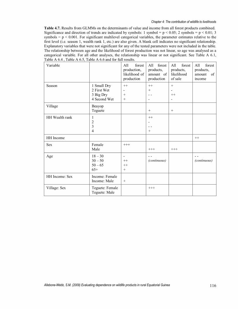
Chapter 4: The contribution of wildlife to livelihoods
Allebone-Webb, S.M. (2009) Evaluating dependence on wildlife products in rural Equatorial Guinea 116
Table 4.7. Results from GLMMs on the determinants of value and income from all forest products combined. Significance and direction of trends are indicated by symbols: 1 symbol = p < 0.05; 2 symbols = p < 0.01; 3 symbols = p < 0.001. For significant multilevel categorical variables, the parameter estimates relative to the first level (i.e. season 1, wealth rank 1, etc.) are also given. A blank cell indicates no significant relationship. Explanatory variables that were not significant for any of the tested parameters were not included in the table. The relationship between age and the likelihood of forest production was not linear, so age was analysed as a categorical variable. For all other analyses, the relationship was linear or not significant. See Table A 6.1, Table A 6.4 , Table A 6.5, Table A 6.6 and for full results.
Variable All forest production, likelihood of production
All forest products, amount of production
All forest products, likelihood of sale
All forest products, amount of income
Season 1 Small Dry 2 First Wet 3 Big Dry 4 Second Wet
++ - + +
++ + - - -
+ - ++ -
Village Beayop Teguete
+
+
HH Wealth rank 1 2 3 4
++ - - - +
HH Income ++
Sex Female Male
+++
+++
+++
Age 18 � 30 30 � 50 50 � 65 65+
- ++ ++ +
- - (continuous)
- - (continuous)
HH Income: Sex Income: Female Income: Male
+
Village: Sex Teguete: Female Teguete: Male
+++

Chapter 4: The contribution of wildlife to livelihoods
Allebone-Webb, S.M. (2009) Evaluating dependence on wildlife products in rural Equatorial Guinea 117
Table 4.8. Results from GLMMs showing the likelihood of harvest and the value of those harvests for forest products. Forest products are divided into animals (bushmeat), fish and wild plants. Significance and direction of trends are indicated by symbols: 1 symbol = p < 0.05; 2 symbols = p < 0.01; 3 symbols = p < 0.001. For significant multilevel categorical variables, the parameter estimates relative to the first level are also given. Where there is a significant interaction between variables, the parameter estimate for both variables combined is shown. A blank cell indicates no significant relationship. Explanatory variables that were not significant for any of the tested parameters were not included in the table. See Table A 6.8, Table A 6.9, Table A 6.10, Table A 6.11 and Table A 6.12 for full results.
Variable Parameter levels
Animal: likelihood of harvest
Animal: amount harvest
Fish: likelihood of harvest
Plant: likelihood of
harvest
Plant: amount harvest
Season 1 Small Dry 2 First Wet 3 Big Dry 4 Second Wet
+ - ++ - -
++ ++ - +
No significant differences
Beay. - - - ++ +
Teg. +++ - - - - - +
Beay. - ++ - - +
Teg. +++ ++ - ++
Village Beayop Teguete
++
HH Income +
Sex Female Male
+++
++
+++
Age +++ Table 4.9. Results from GLMMs showing the likelihood of income and the amount of income for forest products. Forest products are divided into animals (bushmeat), fish and wild plants. Significance and direction of trends are indicated by symbols: 1 symbol = p < 0.05; 2 symbols = p < 0.01; 3 symbols = p < 0.001. For significant multilevel categorical variables, the parameter estimates relative to the first level are also given. Where there is a significant interaction between variables, the parameter estimate for both variables combined is shown. A blank cell indicates no significant relationship. Explanatory variables that were not significant for any of the tested parameters were not included in the table. See Table A 6.13, Table A 6.14, and Table A 6.15 for full results.
Variable Parameter levels
Animal: likelihood of
income
Animal: amount of
income
Fish: likelihood of
income
Plant: likelihood of
income
Season
1 Small Dry 2 First Wet 3 Big Dry 4 Second Wet
+ - ++ - -
Not analysed (n < 20 selling)
No significant differences
Village Beayop Teguete
+
HH Income + +
HH Wealth rank 1 2 3 4
++ + - - -
Sex Female Male
+++

Chapter 4: The contribution of wildlife to livelihoods
Allebone-Webb, S.M. (2009) Evaluating dependence on wildlife products in rural Equatorial Guinea 118
Table 4.10. Results from GLMMs showing determinants of value and income from agricultural harvest. Significance and direction of trends are indicated by symbols: 1 symbol = p < 0.05; 2 symbols = p < 0.01; 3 symbols = p < 0.001. For significant multilevel categorical variables, the parameter estimates relative to the first level are also given. Where there is a significant interaction between variables, the parameter estimate for both variables combined is shown. A blank cell indicates no significant relationship. Explanatory variables that were not significant for any of the tested parameters were not included in the table. See Table A 6.16, Table A 6.17, Table A 6.18 and Table A 6.19 for details.
Variable Level Likelihood of production
Amount of harvest
Likelihood of income Amount of
income
Season 1 Small Dry 2 First Wet 3 Big Dry 4 Second Wet
+ - - ++ ++
Beay. + - ++ +
Teg. + - - - ++
Beay. + - - - +++ - -
Teg. - - - - - - - ++
Beay. +++ ++ + -
Teg. - - - - - - - - -
Village Beayop Teguete
+
Wealth Rank 1 2 3 4
- + ++ - -
HH head sex Female Male
+
Age 18-30 30-50 50-65 65+
- + ++ +
+++ (continuous)
- - ++ ++ +
Sex Female Male
+++ +++ +++ +
Table 4.11. Results from GLMMs showing determinants of likelihood and amount of income from trade. Significance and direction of trends are indicated by symbols: 1 symbol = p < 0.05; 2 symbols = p < 0.01; 3 symbols = p < 0.001. For significant multilevel categorical variables, the parameter estimates relative to the first level are also given. A blank cell indicates no significant relationship. Explanatory variables that were not significant for any of the tested parameters were not included in the table. See Table A 6.20 and Table A 6.21 for details. Variable Level Likelihood of trade Amount income from trade
Season 1 Small Dry 2 First Wet 3 Big Dry 4 Second Wet
+ ++ - +
HH income + +++
HH head education None Primary Secondary Higher
- - - + ++
HH head sex Female Male
+
Age -

Chapter 4: The contribution of wildlife to livelihoods
Allebone-Webb, S.M. (2009) Evaluating dependence on wildlife products in rural Equatorial Guinea 119
4.5 Discussion
Forest products contribute a significant value and income to many people in both villages. Between
the two communities, as expected and reflecting differences in other studies (e.g. Starkey 2004),
people in the more remote Teguete earned less in total, and more from forest livelihoods, of which
income from bushmeat was the most important. The greater accessibility to markets and traders
mean that producers and village traders in Beayop can command higher prices than in Teguete, and
have more opportunities to sell processed goods, generating higher incomes from trade and
agriculture. Greater prices and sales opportunities for agricultural goods in Beayop may also drive
the higher agricultural production seen in that village.
Despite the higher total bushmeat hunting levels, hunter offtake per week, and access to forest
resources in Teguete, the higher prices for bushmeat and access to traders in Beayop mean that both
trappers and gun-hunters earned higher average annual incomes in Beayop. This is to be expected �
in a village with higher average incomes, and more access to alternative incomes, the income from
hunting should be higher to make it an economically attractive activity. The data do reflect that
these villages are not specifically hunter villages, and the average annual incomes from hunting
(gun-hunters and trappers in both villages (US$510 in Beayop and $440 in Teguete) are far less
than those reported by Kümpel (2006) in a hunter village (Sendje) two years earlier, where hunters
earned a mean annual income of $1019 (my currency conversion using 2008 exchange rates). Given
the higher percentage of people hunting in Sendje, the total contribution of hunting income to
villages shows an even greater gap (~$700/person/year in Sendje for all people in the village,
compared to $315 in Beayop and $482 in Teguete). These differences must also be due to the low
transport costs to Bata from Sendje. All these wages are far below the Equato-Guinean annual
minimum wage of $2130/year, but in Teguete and Beayop are equivalent to the $400-700/year
reported earned by trappers in Central Africa Republic, the difference being that in CAR this is
similar to the minimum wage (Noss 1998). Income from gun hunting was significantly higher than
that from trapping, and this is likely to be due to higher value species being killed, preferred species
being targeted and carcasses less likely to be rotten (see chapter 6). Other studies have found guns
to be the hunter method of choice for hunters selling a large proportion of their catch (Dethier 1995;
Auzel & Wilkie 2000).
Average annual wages earned from wild fish and plants are much lower than this. Unsurprisingly,
potential and actual income from wild fish is probably correlated to proximity of water sources in
Equatorial Guinea. The regular incomes from fishing reported previously (Cogels 1997; Cayuela

Chapter 4: The contribution of wildlife to livelihoods
Allebone-Webb, S.M. (2009) Evaluating dependence on wildlife products in rural Equatorial Guinea 120
Serrano et al. 2000) must be in part due to the close proximity of large rivers at these sites,
something that neither Beayop of Teguete have (although Beayop has a medium sized river). The
large income and trade in edible wild plants reported in other parts of west and central Africa
(Ndoye et al. 1998), are not reflected in this study. The two wild fruit species most commonly
reported in other countries, bush mango and African plum, are both are harvested (although not
cultivated) in both villages, and both are sold in urban markets in Bata and Ebibeyin. However,
extremely few are sold in the study villages, and those that are, are sold and consumed locally. This
disparity reflects a general lack of entrepreneurship in the country (as reported in Kümpel 2006),
possibly due to low education levels and investment power in many rural areas. This is also
associated with falling agricultural production, and consequently agricultural incomes, over the last
30 years. The trade in non-edible wild plants of low value is common across men in both villages.
However, without significant changes in production, these have little potential for increasing
incomes substantially. The production of rattan furniture gains high incomes for the two men who
produce it, but they are already reporting a visible reduction in rattan available in the forest, an
observation mirrored in villages closer to Bata (Sunderland et al. 2004). The production of small
artisanal items by the (particularly elderly) men in the village is vital to this group who often have
no other income, but the average income earned and market for goods are both very low. However,
palm wine (also usually produced by men), has more potential. There is a large demand in the
village as it is the cheapest alcohol available, is widely liked, and other countries, such as DRC,
have shown that traders can earn significant incomes from palm wine trade (traders earned
US$166/month, above the gross national product per capita in DRC, Ndoye & Awono (2005).
In both villages, there are large differences in the production and income gained by males and
females, but particularly between the income of men and women in Teguete. Women in Teguete on
average earn only 56% of the average male income, despite producing 88% of livelihood value. In
Beayop women earn 84% of the average male income, and produce 90% of the production value.
This is chiefly due to the maintenance of a strict gender divide in the livelihood activities commonly
followed, whereby females cultivate all staples for the family, while men pursue livelihoods which
often have more earning potential. Paid work is also more likely to go to men, and this is probably
mainly due to lower education levels for females, in part because of the cost of education beyond
primary level (children have to be sent to larger urban areas to live with relatives). The exception is
in the trade of processed goods, and where there is a market for these goods (such as in Beayop),
women can make a reasonable profit, earning nearly half their average incomes from trade,
compared to men who earn 17% of average income from trade. In comparison, women earn an

Chapter 4: The contribution of wildlife to livelihoods
Allebone-Webb, S.M. (2009) Evaluating dependence on wildlife products in rural Equatorial Guinea 121
average 37% of income from trade in Teguete, and men 11%, but the absolute incomes are much
lower in Teguete.
The positive relationship between household wealth and bushmeat harvest reported elsewhere (de
Merode et al. 2004), is also seen in this study. Wealthier hunters gain more income per hunter from
bushmeat in both villages, probably due to harvesting a higher amount of bushmeat per trip, and
being more likely to sell bushmeat when they do catch it. However, averaged across all people
within a wealth rank, bushmeat provides the greatest income for the poorest households. The
evidence shows that this is probably made up of a large number of poor hunters harvesting small
amounts of bushmeat that they are more likely to consume at home. In addition, poorer households
are less likely to earn money from any other livelihood (particularly trade and paid work), so
income from the forest is a greater proportion of their total income, and makes up over 90% of the
income earned by the poorest households in Teguete (compared to 39% for the population as a
whole) and 44% in Beayop (compared to 14%), and this is virtually all from bushmeat.
Seasonally, total production is least in the 2nd and 3rd seasons, known as the �hungry season� and the
long dry season respectively, and this is reflected in a lower income in Teguete. Much of this
difference is due to a lower agricultural production in the 2nd season (when none of the major peanut
or calabaza crops are harvested) and the 3rd season (when the 2nd, smaller, peanut crop is harvested),
coupled with a high production of forest plants in the 1st season (when most of the forest fruit trees
are in season). It is not clear if these deficits are compensated for by other livelihoods, although
men may have less opportunity to pursue other livelihoods such as hunting in the 2nd season, due to
the need to clear fields at this time. As with previously, results on the seasonal differences in
production and income should be treated with caution as they reflect only differences occurring
during the study year. Without additional data, it is difficult to say whether these are useful
predictors for other years, as annual variation in seasonality could affect livelihoods.
Due to the fact that some forest products are currently never sold in either community, and were
consequently not given a monetary value, this study may underestimate the value of forest products.
Products not valued include firewood which is a valuable NTFP in other central Africa countries
(Biloso & Lejoly 2006).
In summary, it seems clear that the forest is providing valuable services to livelihoods in both
villages. Women in the rural village of Teguete gain around half of the value of all goods produced
from the forest and although very little of this is sold, it is contributing greatly to household

Chapter 4: The contribution of wildlife to livelihoods
Allebone-Webb, S.M. (2009) Evaluating dependence on wildlife products in rural Equatorial Guinea 122
production. For all people, poorer households gain a lower income, but of this a greater amount and
a greater proportion is from forest goods, with bushmeat providing almost all income to the poorest
people in Teguete and nearly half in Beayop. Given that neither village �specialises� in hunting, and
that Beayop at least is has access to urban areas and is not considered to be adjacent to any
particularly wildlife-dense forests, the large income by the poorest people has large implications for
the rest of Río Muni. Teguete and Beayop between them represent a reasonably large part of the
spectrum of forest and market access by villages. Consequently we must assume that the poorest
households in many other villages in Río Muni may also be earning 45-95% of their income from
bushmeat hunting.

Chapter 5.
Evaluating dependence on
wildlife for vulnerable
people and at vulnerable
times

Chapter 5: Evaluating dependence on wildlife for vulnerable people and at vulnerable times
Allebone-Webb, S.M. (2009) Evaluating dependence on wildlife products in rural Equatorial Guinea 124
5.1 Abstract
To assess dependence on forest products, as opposed to simply the use of wildlife for consumption
and income, the proportion of consumption, production and income from different sources was
quantified for the most vulnerable households and seasons, and compared to the rest of the
community and to other seasons. In this chapter, I assess the food security of households in both
study villages, by measuring the frequency of use and the severity of household coping
mechanisms. Vulnerable households are identified as being the least food secure, and these are also
the poorest households, with the lowest ratio of productive adults to dependents. Vulnerable
households are also less livelihood secure in that they have a lower diversity of livelihoods and
fewer income sources. The most vulnerable season is shown to be the second season when data
from previous chapters demonstrates that consumption and income are among their lowest, and
when children under five are most likely to weigh proportionally less. The poorest and least food
secure households gain a significantly greater proportion of income and production from forest
products than other households, but do not consume significantly different sources of food.
Agricultural income is significantly lower during the lean season and although households do not
show a significant difference in other livelihood activities during this season, this reduction may
impact poorer households the most, both in total income and in their ability to earn money from
alternative sources. Thus, this chapter provides strong evidence that the most vulnerable households
are more dependent on forest products for both income and livelihoods.
5.2 Introduction
In this chapter, I move beyond the measurement of wildlife use for consumption and income as
described in chapters 3 and 4, to broader indicators of food and livelihood security in order to assess
the use of wildlife resources as a safety net, providing food and livelihoods to the most vulnerable
households, and in the most vulnerable seasons. I assess the proportion of food, production and
income provided by forest products compared to other resource types, and evaluate which resources
are most important to the most insecure groups and at the most vulnerable times of year.
5.2.1 Beyond food consumption and income
As demonstrated in chapters 3 and 4, the use of wildlife resources for consumption and livelihoods
is extensive in both Teguete and Beayop. However, it is through the evaluation of the use of wild
foods as a safety net that we begin to assess people�s dependence on wildlife products. Wildlife

Chapter 5: Evaluating dependence on wildlife for vulnerable people and at vulnerable times
Allebone-Webb, S.M. (2009) Evaluating dependence on wildlife products in rural Equatorial Guinea 125
resources may act as a safety net in a number of ways, including through their potential to provide
food or income during times of stress.
To assess the ability of wildlife to reduce vulnerability to food shortages, we have to look beyond
simply food consumption, to the role of wildlife in food security. Wild foods can contribute to food
security by providing a �back-up� supply of food when people most need it, so protecting
individuals, households or communities from extreme fluctuations in consumption. This may be
during a lean season (Fleuret 1979; Chambers et al. 1981), during times of stress such as famine,
conflict or disease epidemics, (Vaughan 1987; de Waal 1988; Sullivan 1998; Draulans & Van
Krunkelsven 2002; Jamiya et al. 2007) or during times of financial hardship � i.e. for the poorest
households (Shackleton & Shackleton 2006). For example, in the Democratic Republic of Congo
(DRC), consumption of wildlife increased by 75% on average during the hungry season (de Merode
et al. 2004). In addition, wild food consumption can lead to a healthier diet, providing access to
valuable nutrients that people may not otherwise have adequate access to, leading to a positive link
between health and wild food consumption (Dounias & Colfer 2008). Others have highlighted the
importance of bushmeat to regional protein supplies and predicted large decreases in availability in
the future (Fa et al. 2003), or shown links with other sources of protein at a regional level, namely
similarly threatened marine fish supplies (Brashares et al. 2004; Rowcliffe et al. 2005).
Similarly, as we look beyond consumption when assessing the value of wild foods to food security,
we need to look beyond total income generation if we are to understand the role of forest products
to sustainable livelihoods. Consequently we need to look at the potential of wild resources to
provide income in times of hardship, and their contribution to diversifying income and production.
A livelihood is considered sustainable when it can �cope with and recover from stresses and shocks,
maintain or enhance its capabilities and assets, while not undermining the natural resource base�
(Scoones 1998), and people are more likely to have a sustainable livelihood portfolio when they
gain income from a range of livelihood sources. Initial results show that wildlife resources may be
important in contributing to livelihood diversification and safety nets (Shackleton & Shackleton
2004), particularly for poorer groups (Vedeld et al. 2007). Rural households may turn to wildlife
sales in response to agricultural shortfalls (Loibooki et al. 2002) and to complement agricultural
production in the lean season or between two crops (Chardonnet et al. 1995; Crookes et al. 2007).
Livelihood diversification is an important strategy in reducing an individual or households
vulnerability to shocks such as crop failure, illness, job loss, or extreme climatic events; with a
greater number or diversity or income sources, the chances of all income sources failing at the same

Chapter 5: Evaluating dependence on wildlife for vulnerable people and at vulnerable times
Allebone-Webb, S.M. (2009) Evaluating dependence on wildlife products in rural Equatorial Guinea 126
time is very low. The poorest people tend to have less diverse income sources and so are more at
risk to periods of very income and unexpected income (Vedeld et al. 2007).
Some institutions have pointed to the similar values of food security and livelihoods approaches,
including a recognition of the temporal nature of food security (shown in the distinctions made
between chronic food insecurity and transitory food insecurity) and livelihoods (shown in the
emphasis on sustainable livelihoods) and the importance of vulnerability in both approaches.
Devereux et al (2004) have reported in detail on the usefulness of livelihoods approaches for food
security monitoring and others have explicitly included livelihoods strategies as one aspect affecting
food security, in a conceptual framework of the latter (Wolfe & Frongillo 2001). Consequently, a
study of the dependence on wild foods should include an investigation of importance of wild foods
in the (albeit overlapping) provisioning of food security and sustainable livelihoods.
Warner (1995) proposed that the degree of dependence of a community on wildlife products is due
to the condition of the resource, its proximity to the community, access rights and restrictions, local
and external demand, and income earning options. For a forest community, this translates to the
condition of the forest and prey populations, distance to the forest, access rights (cost of permits or
fines), local and larger market demand and consequently price of wild resources and alternatives
(which depends a lot on the presence of traders in more isolated villages), alternative livelihoods
available, and different individual, cultural and community attitudes to wildlife, attitudes to work
and food preferences. The greater access to relatively less exploited forests in Teguete, coupled with
the lower availability of alternative livelihoods suggests that people in Teguete are more likely to
depend on wildlife than those in Beayop. In addition, although bushmeat is most commonly referred
to in the context of food security and livelihoods, it is wild plants (de Merode et al. 2004) and fish
(FAO 2006) that are often more important to the extreme poor or food insecure, particularly for
women and children, so we might expect a greater dependence on forest plants than bushmeat.
5.2.2 Food security indices
Given the multi-faceted nature of food security, it is difficult to measure using a single metric, and a
recent international symposium concluded that a suite of indicators was needed to cover different
dimensions of food insecurity (IFPRI 2002; FAO/FIVIMS 2003). These methods include traditional
measurements such as nutritional intake and child growth data, as well as other indicators such as
identifying the presence and common use of �household coping mechanisms� (Corbett 1988) and
the similar rapid �comparator indicator questionnaires�, as well as famine vulnerability assessments.

Chapter 5: Evaluating dependence on wildlife for vulnerable people and at vulnerable times
Allebone-Webb, S.M. (2009) Evaluating dependence on wildlife products in rural Equatorial Guinea 127
This broadening of the suite of indices addresses the widely argued necessity for qualitative and/or
more rapid measures of hunger and food security. I use elements of all these measurements except
famine vulnerability assessments, which were deemed not appropriate due to the regional scale of
these assessments (and so beyond the scope of this study) and due to the very low likelihood of
extreme shortages of food supplies in the study site.
The measurement of food coping strategies as an indicator of food security is based on the principle
that a that a simple set of questions, representing the most common coping behaviours relied on by
people in the community when there is insufficient food or money to buy food, can be determined
by focus groups. These coping strategies can then be ranked or weighted and the frequency that
each strategy was used assessed for each household or community. The combination of the severity
and frequency of use for each strategy, summed across all strategies, then results in a quantitative
score that allows identification of vulnerable households, or monitoring over time (Maxwell 1996;
Maxwell et al. 1999). Subsequent studies have used variations on this type of indicator, usually
including questions on one or more of the following types of strategies:
• dietary change strategies, such as consumption of less expensive and/or less preferred
foods;
• food-seeking strategies, including increasing in the amount of food available in the short
term (e.g. by borrowing food or money, foraging for different types of food, harvesting
immature crops, etc.);
• rationing strategies, such as eating less often or smaller amounts, to prioritise feeding of
certain family members (e.g. vulnerable members such as children, �maternal buffering�; or
working members of the family), or to even pass entire days without eating;
• household structure strategies, such as action to decrease the number of people to be fed
in the short term (e.g. by migration, or sending children to live with relatives).
Questions on all four types of strategy were combined in the Coping Strategies Index developed by
the FAO (Maxwell et al. 2003) as a quick and easy tool for food security assessment, particularly in
Africa. Other studies have used the measurement of coping strategies in a range of countries and
situations, including in South Africa (Oldewage-Theron et al. 2006), as an assessment of food
security among households with HIV/AIDS (Senefeld & Polsky 2006), Bangladesh (Frongillo et al.
2003; Park 2006), Malasia (Zalilah Mohd & Khor 2004), Sri Lanka (Senaratna 2006) and Kenya
(Malleret-King 2000). Rapid comparator indicator questionnaires such as the widely used FAST
system developed in the USA (Wolfe & Frongillo 2001; Hall 2004), adapted questionnaires in

Chapter 5: Evaluating dependence on wildlife for vulnerable people and at vulnerable times
Allebone-Webb, S.M. (2009) Evaluating dependence on wildlife products in rural Equatorial Guinea 128
Bangladesh (Coates et al. 2003; del Ninno & Dorosh 2003) and the more recently developed food
access measurement (Coates et al. 2007) incorporate questions from some of these strategy groups,
namely dietary change and rationing strategies, with additional questions on hunger and perceptions
of vulnerability and anxiety. Other studies have found dietary diversity a useful indicator of
micronutrient deficiencies, particularly in vulnerable groups such as women of a reproductive age
(Arimond et al. 2008). The assessment of short and long-term accumulation strategies, using similar
methodologies, has been used to provide additional information in some studies (Malleret-King
2000; Senaratna 2006).
5.2.3 Anthropometric measures
In this chapter, to identify the most vulnerable season, I use infant (under-fives) anthropometric data
collected over five years in Teguete. The use of child nutritional indicators such as weight, height
and age ratios is one of a suite of traditional measures often used to measure food security (Shetty
2002). Low weights and heights are often a sign of malnutrition, with wasting (thinness or a low
weight-for-height) being particularly associated with acute hunger, while stunting (shortness or a
low height-for-age) is commonly associated with chronic hunger. Being underweight (low weight-
for-age) can be due to wasting or stunting and is a reflection of general malnutrition.
The use of child nutritional indicators less useful as a food security measure at the individual level
because low weight or malnutrition can be due to a number of reasons, particularly illness and poor
health-care practices, as well as poor food consumption. Indeed, health, wealth and food
consumption all influence, and are influenced by, each other. Poor families are less likely to be able
to afford health care and food, and so are more likely to become ill. In turn, sick adults are less able
to work and so provide food or money to the household, and sick children require care, preventing
adults from working. People with inadequate diets are less able to work, and are more vulnerable to
disease and illness. An additional consideration is that weaker members of a household are often
buffered by other household members (mothers may particularly buffer young infant consumption),
so minor food shortages may not impact young children and therefore an absence of low child
weights does not imply that all members of the household are equally well nourished. Finally, low
infant weight is usually a reflection of poor food consumption, rather than a cause of it, so
anthropometric data is not very useful as a diagnostic tool for the causes of food insecurity.
However, in this case, we are only looking for reflections of changes in food insecurity between
different seasons. With a large sample size (as used here) and repeated measurements of the same

Chapter 5: Evaluating dependence on wildlife for vulnerable people and at vulnerable times
Allebone-Webb, S.M. (2009) Evaluating dependence on wildlife products in rural Equatorial Guinea 129
individuals across different years, consistently relatively lower child weights within a particular
season are likely to represent a vulnerable season for all members of the community.
5.2.4 Vulnerable seasons and households
Previous chapters have indicated the second season, and to some extent the third season as being
when households are potentially at greater risk from food and income shortages. Focus groups
discussing the agricultural calendar identified the second season as being the �hungry� season,
although this was as much to do with the large amounts of work needed to be done in the fields, as
the lack of foods being harvested. It is also the time when stores of protein staples such as peanuts
are most likely to run dry (Chapter 2). Total food consumption was lowest in the second and third
seasons (Chapter 3) and in Teguete at least, total production and income were again lowest in the
second season, followed closely by the third season (Chapter 4). Production and income in Beayop
were less consistent, but the second season did show the lowest production (albeit with very little
variation between seasons) and the second lowest average income (Chapter 4). Consequently, if
people do depend on wildlife resources as a seasonal safety, we would expect them to use it in
greater proportions during the second or third seasons.
In this chapter, I identify the most vulnerable households as those using food coping strategies most
frequently. I identify which season is most likely to be vulnerable to lower food and income
supplies by analysing data on child weights and ages to assess when children are most likely to
weigh relatively less. Having ascertained the most food insecure households and seasons as far as
the data allow, I then analyse which food sources and livelihoods provide the greater proportion of
food, production and income for the most vulnerable quartile of households compared to the rest of
the community. Finally, I analyse which food and livelihood sources provide the greatest proportion
of food production and income in the most vulnerable season, compared to other seasons.
5.3 Methods
To identify the most vulnerable households within each study village, I quantified the use and
severity of food coping strategies within the household as an indicator of food security, taking food
insecurity as a more accurate measure of vulnerability than simply low food consumption. This was
followed by an analysis of the characteristics of the least food secure quartile of households in each
village, which is used both as an indicator of the validity of the approach (i.e. food security is
consistently, but not solely, related to household wealth measures in most studies), and as a
descriptor to characterise the least food secure households (e.g. for assessment of any demographic

Chapter 5: Evaluating dependence on wildlife for vulnerable people and at vulnerable times
Allebone-Webb, S.M. (2009) Evaluating dependence on wildlife products in rural Equatorial Guinea 130
correlates of food security). Wealth rank is used as a second indicator of household vulnerability,
and it is assumed that a community�s perception of household wealth is likely to consider a wide
range of factors beyond income alone (see Chapter 2 for discussion). Finally, I assess one aspect of
livelihood security, namely income diversity, to examine whether the households identified as the
poorest and least food insecure are also livelihood insecure.
5.3.3 Data Collection
Food Coping Strategies
The frequency of use of a range of food coping strategies was assessed twice: once in April 2005
(the 2nd season) and once in February 2006 (the 1st season). In 2005, focus group discussions were
held beforehand to identify the commonly used coping strategies, and then questionnaires were
conducted at each household to ask how frequently they had used this strategy over the previous
two months, and how severely they ranked those strategies that they had used.
In 2006, the focus group discussions were repeated, but this time in greater depth, to investigate
some of the ideas behind different coping mechanisms, and to get a consensus on the order of
severity of the various strategies. In each discussion group, the coping strategies were written on a
card (with pictures also illustrating the strategy, for those who couldn�t read). The four female
respondenets were asked to review the strategies and new ones were added where appropriate. They
were then asked to put the strategies in order of which strategy was the least serious (i.e. what they
would do first in times of food and money shortages), up to the most serious strategy (i.e. the last
resort) that they would only do if all other options had been investigated. Discussions were held
until the four women in each group arrived at an agreed order, and repeated three times in each
village. Focus groups also discussed long term coping strategies, but all strategies that were
discussed (such as migration, selling house, etc.) were deemed not possible (in the case of house
sales), or not appropriate by respondents. For example, the closest to migration anyone got was
moving from the city and back to the village, when the search for a job in the city had failed, so for
some people, living in the village was already a coping strategy.
Questionnaires were then conducted with all households, this time asking only questions on the
frequency of strategy use (and not severity). Data were collected on accumulation strategies, both
within the focus groups and questionnaires, but the results were found to be more an indicator of
wealth, and didn�t add any real information to the study, so these results have not been reported.

Chapter 5: Evaluating dependence on wildlife for vulnerable people and at vulnerable times
Allebone-Webb, S.M. (2009) Evaluating dependence on wildlife products in rural Equatorial Guinea 131
Questionnaires also included a question on the frequency of anxiety over food supplies, in line with
previous food security questionnaires (see introduction).
The timings of the two food security questionnaires were somewhat borne out of necessity but also
choosen to reflect different seasons within the year, including the season identified as the �hungry�
season by agricultural focus groups. Given that not all seasons were assessed (and only one score
used), data from the food security questions were used only to distinguish between households, not
between seasons.
Food security score
The frequency of use of each strategy (as represented by the proportion of days on which it was
used over the previous two months) was multiplied by the severity of that strategy (as given by the
consensus in the 2006 focus groups, a high score being more severe), to give one number per
strategy. These were summed, to give one score per household per survey. This score is referred to
as the food security score for each year, with a higher value denoting a less food secure household.
The score for 2006 was used in data analysis as it was considered more accurate, due to a revision
of the questions.
Anthropometric measurements
In both villages, all members of the village that desired were weighed and measured in February
2006, according to standard protocols, as described by de Onis (2004). Children under 16 were only
measured with parental consent and presence. Children under five were weighed and measured by
local health care workers, with parental consent and presence. In addition, permission to use
Teguete health centre records was obtained. These records contain the monthly weights and ages of
most under-fives in the village for the period 1996-2000. After this date, the records are incomplete
or non-existent, due to illness of the health worker at the time. Individuals were identified by name
and by household code in the health centre records (their coding). Date of birth was recorded with
weight, and these were checked against other health centre records, for consistency, as well as with
our own records where the individual could be identified as someone living in the village. Height
was not measured for many of the health centre records, partly due to a lack of a measuring rule
(and so the inability to measure supine length) and for this reason weight-for-age data is used here.
This is also the most widely used metric in developing countries, and although it cannot distinguish
between wasting and stunting, it does represent a combination of both these aspects, and has a high
positive predictive value as an indicator for child malnutrition in developing countries (WHO
1995). WHO Anthro 2005 software (WHO Anthro 2005 Beta version 2006) was used to convert

Chapter 5: Evaluating dependence on wildlife for vulnerable people and at vulnerable times
Allebone-Webb, S.M. (2009) Evaluating dependence on wildlife products in rural Equatorial Guinea 132
weight and age data into a weight-for-age z-score (WAZ). The z-score expresses values as a number
of standard deviations above or below the reference mean, giving a linear scale with a mean of 0
and standard deviation of 1. The reference mean used by the programme is taken from data
collected from breast-fed infants across six countries in five continents between 1997 and 2003.
Individual and household level variables
Village, household income, household fixed wealth, wealth rank, number of productive adults
(defined as healthy adults aged 18-65), number of productive females, presence of productive males
(yes/no), number of people in the household (household size), proportion of productive adults in the
household, proportion of productive females in the household, sex of household head, education
level of household head, sex, age, education and season were used as household and individual-
level explanatory variables, and analysed with respect to food security scores. See Chapter 2 for
data collection and analysis methods.
Food consumption
The number of calories consumed from different food sources was recorded from 24 food recall
questionnaires, across the year. Food sources were split into four categories: agriculture, forest,
bought, and gifts, according to where or how the household obtained that particular food item. The
proportion of calories consumed from each source was calculated for each household for each
sample day, and these proportions were averaged for the year and for each season separately. See
Chapter 3 for details.
Income and production
The value of all products and income produced or earned from different sources was recorded from
24 food recall questionnaires, across the year. Income and product sources were split into four
categories: agriculture (�produced�), forest, trade and paid work, according to where or how the
household obtained that particular product or income. The value of all products was taken as the
value of anything earned, produced or harvested. Income was taken as the value only of those
products actually sold (or the profit made on those items that were traded) or income. The
proportion of product value and income from each source was calculated for each household for
each sample day, and these proportions were averaged for each season, and then for the year. See
Chapter 4 for details.

Chapter 5: Evaluating dependence on wildlife for vulnerable people and at vulnerable times
Allebone-Webb, S.M. (2009) Evaluating dependence on wildlife products in rural Equatorial Guinea 133
5.3.4 Data Analysis
All data were analysed in R, version 2.6.2 (R Development Core Team 2007). Models were
simplified to obtain the minimum adequate model by fitting the saturated model and then
comparing models with progressively simplified fixed effects using anova. Significance was taken
as p<0.05.
The variation in food security score with household characteristics was analysed with a linear mixed
model using the lme4 library (Bates & Sarkar 2007). The household food security scores from both
2005 and 2006 were used where available. Year and household nested within village were specified
as random effects. Fixed effects were all the household level variables (as detailed above), as well
as season, year (2005 or 2006) and village. Explanatory variables were transformed to give Normal
distributions where appropriate (see Chapter 2 for details).
The variation in WAZ score was analysed in two sets of data. The first included only the data for
which the individual was currently in the village and could be identified, and so household level
variables could be assigned, as well as individual variables (sex and age), year of measurement and
season of measurement. The second analysis included all WAZ scores, and only individual
variables, year and season. For this second set of data, individuals and households were identified
and coded from the health centre records, allowing individual and households to be fitted as random
effects, despite not knowing exactly which household the health centre code referred to. In this way,
year and individual nested within household were specified as random effects in all analyses. Only
data from Teguete were used, so it was not necessary to specify village as a random effect.
In order to analyse the difference between the food sources of the most food insecure and other
households, the households in each village in the least food secure quartile (as measured by food
security score) were identified. The proportion of calories from each of the four sources
(agriculture, forest, bought, gifts) was averaged across the whole year for each household. The
composition of the food sources for the least food secure households was compared to the
composition of the food sources for the rest of the population using compositional data analysis, and
the library �compositions� in R (van den Boogart et al. 2006). Data were put into the vector class
�acomp�, the centred log ratio transformation taken (using the �clr� function) and analysed with a
multivariate analysis of variance (manova) to show the significance of food security quartile and
village. This was done using a two level factor - quartile 4 (the least food secure) and quartiles 1-3
lumped together. The same was done to compare the most vulnerable season with other seasons.

Chapter 5: Evaluating dependence on wildlife for vulnerable people and at vulnerable times
Allebone-Webb, S.M. (2009) Evaluating dependence on wildlife products in rural Equatorial Guinea 134
To analyse the difference between the livelihood and income sources of the most food insecure
households, the average proportion of production value from each livelihood source (forest,
agriculture, paid work and trade) was calculated for each household in each season, and the average
value per household taken as the average across all four seasons. The composition of the proportion
of value from all livelihoods for the least food secure quartile of households in each village was
compared to the composition of the production sources for the rest of the population in the same
way as for the food consumption data. The same was done to compare the most vulnerable season
with other seasons. The process was repeated for income from each livelihood source, and to
analyse the poorest households (as identified by the bottom household wealth rank) compared to
other households in the community.
5.4 Results
5.4.1 Identifying the most vulnerable households
Identifying and ranking Food Coping Strategies
The strategies identified during the focus groups were as follows (in order of increasing severity):
• �pass the whole day without eating meat or fish�: This happens all the time and isn�t
considered a problem. To go for a whole month without eating meat or fish is not
uncommon. However, there was some confusion within the focus groups as to the definition
of meat or fish, with some women not counting smoked fish as proper fish. We agreed on
counting all meat and fish (including smoked) as meat and fish, and ensured that this was
specified in each interview.
• �the mother eats less food to ensure that the children have enough�: One woman explained
that during the evening meal, everyone eats equally. If there is enough food, everyone eats
again the next morning. If there isn�t enough food then only the children eat and the mother
goes into the fields to look for food without having breakfast (or lunch). This is a common
strategy (buffering the vulnerable members of the household), and is also one of the
strategies identified in the USA and Bangladesh questionnaires (Wolfe & Frongillo 2001;
Hall 2004). However, to avoid biasing results towards to the numerous households without
children, this question was asked but not included in the analyses.

Chapter 5: Evaluating dependence on wildlife for vulnerable people and at vulnerable times
Allebone-Webb, S.M. (2009) Evaluating dependence on wildlife products in rural Equatorial Guinea 135
• �ask for a loan or gift of food�: Groups reported that this happens commonly, and is usually
small things like a bar of cassava, which would then be returned the next time that that
household made cassava themselves.
• �when there is no soap, don�t buy more due to a lack of money�: The most common and
cheapest soap was used to clean clothes and pots, as well as people.
• �when there is no petrol (kerosene), don�t buy more due to a lack of money�: This was
deemed only slightly less serious than having a lack of salt, with the reason given that you
couldn�t prepare food without salt for more than three days in a row, but you could sleep in
the dark. However, the order changed when there were many ants around when a lack of
petrol became more severe than a lack of salt. This was because petrol was used with
varying success to ward off large swarms of ants heading towards the kitchen. This became
a serious problem about once a year, when large parts of the village would be overrun with
ants, which would then eat any food in their path.
• �when there is no salt, don�t buy any more due to a lack of money�: See above.
• �eat only once a day�: Respondents noted that this is quite rare.
• �ask for a loan or gift of money�: This was deemed one of the most severe strategies, but
group members said that this depended on whether you were working and what the
likelihood was that you would have money to pay back the loan quickly, as well as on the
amount you were borrowing. So, for someone with a salary, or whose relatives regularly
sent cash, to borrow money was not a big issue. In contrast, someone with no regular cash
income would only borrow money (and would probably only be lent money) under extreme
circumstances, such as needing money to buy medication or go to hospital. More common
was asking for credit at the local shop, and this was viewed as far less serious, probably
because the amounts involved were very small (usually 100-500 cfa). Neither asking for a
loan, or getting credit from the shop, was included in the calculations due to the large
potential differences in the amounts, and because the severity was likely to be very different
depending on the wealth of the person (i.e. a wealthy person could borrow money or claim
credit at the shop every morning, and probably pay it back every evening, without any
problems).
• �go all day without eating�: This is extremely rare.

Chapter 5: Evaluating dependence on wildlife for vulnerable people and at vulnerable times
Allebone-Webb, S.M. (2009) Evaluating dependence on wildlife products in rural Equatorial Guinea 136
Questions were also asked on borrowing fish or meat, and mothers eating less fish or meat to ensure
that children have enough of these foods, but these questions (being very similar to questions on all
food types) seemed to confuse people, so they were dropped from the 2006 questions. Other
strategies that were mentioned were the harvesting and sale or consumption of more agricultural
food or more wild food. While these seemed to be important mechanisms for consumption and
income smoothing, it was less easy to see how these could be measured, particularly given that they
were long-term food harvest strategies for a large number of households; without regular
questionnaires over a number of seasons and years, it would be impossible to distinguish between a
regular activity and a short-term response to a food shortage. Consequently, these questions were
not included in the questionnaire. The purchasing of salt, soap and petrol was originally raised in
focus group discussions on short term accumulation strategies, and these items were identified as
among the first that would be bought with any money available (if the household didn�t already own
them). After further discussion, it was decided that a lack of these items was a better indicator. This
was particularly true given that these items were bought in a wide range of quantities (i.e. people
could buy a cup of salt or a 5kg sack of salt), so measuring the frequency of purchase would be
meaningless.
In 2005, each household was asked to rank the severity of the strategies that they had used (Table
5.2). In 2006, the severity rank was instead decided in three focus groups in each village, with
strategies ranked according to how serious, or drastic a strategy was (i.e. the strategies that people
were most likely to avoid until all other options were exhausted were deemed the most severe). The
results are shown in Table 5.1 and show generally a great deal of agreement between focus groups
and villages. The biggest difference was that people in Beayop viewed borrowing money as far less
serious than people in Teguete. After discussion, it was explained that if you had a regular income,
or had family who had money, it didn�t matter if you borrowed money, as you were likely to be able
to pay it back quite quickly. Consequently, it was for the poorer households that borrowing money
was the most serious, and in Teguete far fewer households had family members earning a regular
monetary income. This, in addition to the large differences in quantity of money that could be
borrowed (which again was not reflected in the questionnaire asking about the frequency of strategy
use) meant that data from this question were not included in the analysis. For similar reasons, we
did not use data on the frequency of gaining credit from the shop. Although this was viewed as less
serious than borrowing money, partly because the amounts involved were often much lower, it was
still reported to be more likely that wealthier households would get credit, partly because shop
owners were more willing to give them credit, and partly because they were more likely to eat shop-

Chapter 5: Evaluating dependence on wildlife for vulnerable people and at vulnerable times
Allebone-Webb, S.M. (2009) Evaluating dependence on wildlife products in rural Equatorial Guinea 137
bought food. The average frequency of use and number of households using each strategy in 2005
and 2006 are shown in Table 5.2 and Table 5.3.
Table 5.1 Severity rankings for the different coping strategies from the 2006 focus groups and the final ranking. 1 = least severe, 10 = most severe (i.e. the strategy most avoided). In B1 and T1 (the first focus group in Beayop and Teguete, respectively), a lack of soap, petrol and salt was not included in the rankings. The final rank shows the rank used in calculations. Strategy 2 was not used in calculations, to avoid biasing results to those households without children (and hence who did not use this strategy). Strategies 4 and 8 were also not used in the calculations (see text for discussion). *The median and mean scores use ranks only from the four discussions where all coping strategies were discussed.
Strategy B1 B2 B3 T1 T2 T3 Median score* Beayop
Median score*
Teg
Mean score*
Final Rank
(2006)
1. The family doesn�t eat fish or meat during the day
1 1 1 1 1 1 1 1 1 1
2. Mother eats less so that the children have enough
2 2 2 2 2 2 2 2 2 X
3. Ask for a loan or gift of other food
3 3 3 3 3 3 3 3 3 2
4. Ask for credit at the shop 4 4 4 4 4 5 4 4 4.25 X
5. When there�s no soap, can�t afford to buy any more
5 5 5 4 5 4/5 4.75 3
6. When there�s no petrol, can�t afford to buy any more
8 7 6 6 7/8 6 6.75 4
7. Family eats only once during the day
6 7 8 5 7 7 7/8 7 7.25 5
8. Ask for a loan or gift of money
5 6 6 6 10 9 6 9/10 7.75 X
9. When there�s no salt, can�t afford to buy any more
9 9 8 8 9 8 8.5 6
10. Nothing eaten all day 7 10 10 7 9 10 10 9/10 9.75 7

Chapter 5: Evaluating dependence on wildlife for vulnerable people and at vulnerable times
Allebone-Webb, S.M. (2009) Evaluating dependence on wildlife products in rural Equatorial Guinea 138
Table 5.2. Coping strategies for 2005 including respondents� severity rankings. No. HH refers to the number of households that report using this strategy in the previous 2 months. Mean score refers to the mean severity ranking (higher scores denoting a more severe strategy). The rank of scores is simply the average severity scores, ranked. (both) indicates both villages combined. 1 Not included in calculations
Strategy No. HH both
Mean severity score (both )
Rank of av. score (both)
No. HH
Beay.
Mean severity
score Beay.
Rank
Beay.
No. HH Teg.
Mean severity score
Teg.
Rank
Teg.
The family doesn�t eat fish or meat during the day
119 1.6 2 48 1.54 2 71 1.66 2
Mother eats less so that the children have enough
56 4.5 7 3 1.33 1 53 4.72 6
Ask for a loan or gift of other food
71 4.6 8 22 1.86 3 49 5.78 7
When there�s no soap, can�t afford to buy any more
58 3.2 3 2 2.5 8 56 3.27 3
When there�s no petrol, can�t afford to buy any more
62 3.7 5 2 2.5 8 60 3.78 4
Family eats only once during the day
48 1.1 1 2 2 4 46 1.02 1
Ask for a loan or gift of money 1
64 4.6 8 25 2.24 5 39 6.10 8
Nothing eaten all day 0 0 0
Mother eats less meat or fish so that the children have enough 1
57 4 6 4 2.25 6 53 4.09 5
Ask for a loan or gift of meat or fish 1
16 3.25 4 12 2.25 6 4 6.25 9

Chapter 5: Evaluating dependence on wildlife for vulnerable people and at vulnerable times
Allebone-Webb, S.M. (2009) Evaluating dependence on wildlife products in rural Equatorial Guinea 139
Table 5.3 Frequency of use for different coping strategies in both villages, 2006. Total no. HH refers to the total number of households replying to this question (note a reduced number for strategy 3, where households with no children have not answered the question). No. HH refers to the number of households reporting use of this strategy at least once. Average frequency refers to the average proportion of days this strategy was used across all households.
Strategy Total no. HH
Beayop
No. HH
Beay.
Average freq.
Beayop
Total no. HH Teg.
No. HH Teg
Average freq Teg
1. The family doesn�t eat fish or meat during the day
99 82 0.328 91 88 0.649
2. Mother eats less so that the children have enough
80 54 0.236 57 41 0.176
3. Ask for a loan or gift of other food 99 59 0.119 91 41 0.090
5. When there�s no soap, can�t afford to buy any more
99 37 0.053 91 24 0.094
6. When there�s no petrol, can�t afford to buy any more
99 49 0.024 91 27 0.095
7. Family eats only once during the day 99 22 0.039 91 38 0.138
8. Ask for a loan or gift of money 99 25 0.006 91 8 0.001
9. When there�s no salt, can�t afford to buy any more
99 28 0.019 91 24 0.068
10. Nothing eaten all day 99 6 0.003 91 6 0.015
Worry about where food for next day coming from
99 44 0.054 91 40 0.088
Aside from the final list of coping strategies, there was some interesting discussion around the
subject of what respondents would do if there were food shortages in the household. They were
asked to describe the sequence of events, from what they would do if there were no food in the
house, going through all the first options, and if each of these in turn were not successful, what the
following action would be. A typical sequence of events in Teguete was described:
• If they don�t have any food in the house, then they look for some in their fields or buy
some.
• If they have no money and the �staple� foods in the field are finished (i.e. their stock of
cassava is used up), then they would ask family members or other people in the village for
food from their fields (e.g. cassava, yams, maize, sugar cane, greens)
• If there is still no food, or they have run out of �sauce� foods (e.g. peanuts, calabaza, bush
mango that are eaten with or without meat, and accompanied by a staple such as cassava),
because they are between harvests, then they might ask to borrow food from other people�s
kitchen stores, or they would go and look for greens (typically found on the edges of fields
and forests), but they would only do this if they have palm oil (also collected from the forest
or fields)

Chapter 5: Evaluating dependence on wildlife for vulnerable people and at vulnerable times
Allebone-Webb, S.M. (2009) Evaluating dependence on wildlife products in rural Equatorial Guinea 140
• If this fails, they would then go to the forest; men would set snares or would fish with rods
or fish-traps, and women would go fishing using �esia� a natural fish poison (only possible
in the dry season), fish traps or hand�held fish nets, �tariyas� (again mainly done in the dry
season), and would continue to eat peanuts and calabaza as the �main food� (i.e. an
undesirable substitute to meat and fish � peanut and calabaza soups are generally eaten with
meat or fish in them).
The women in Teguete raised other points. The main issue was that the lack of money is due to a
lack of food sales (i.e. lack of market opportunities). Some women in the village have six fields of
cassava, but can�t sell it as there aren�t enough people in the village to buy it, and nobody comes
from Bata (the main town) on a regular basis. The women in Beayop did not have this complaint,
but said that most women who wanted to sell cassava could sell it on the side of the road to passing
cars. They also pointed out that the people in Cogo (a town on the south-west coast, bordering
Gabon) had it easy because traders visit from Libreville and buy not only cassava, but even the
leaves used to wrap up the cassava, and consequently, the women in Cogo are rich like the men.
They also said that if someone is ill, they still work, but they just do less (i.e. have a smaller field).
People in Beayop expressed an appreciation of the forest slightly differently, saying that the people
of Ebibeyin and surrounding areas (where population density is much higher), are very unlucky as
they have no forest, and consequently eat much less meat and fish. One older man also stated that in
the Ebibeyin region, if a man has no job, he cannot try and make something from the forest, so
people are poorer.
5.4.2 Characteristics of the least food secure households
On all three measurements of wealth, poorer households in both villages are significantly less food
secure; household income (deviance change = 64, p < 0.0001), household fixed wealth (deviance
change = 14, p < 0.01) and wealth rank (deviance change = 10, p < 0.05, Table A 8.1). In addition,
less food secure households have a significantly lower proportion of productive adults in the
household compared to the total number in the household (deviance change = 22, p < 0.0001) and
Teguete was significantly less food secure than Beayop (deviance change = 6, p < 0.05). The
correlation between food security score and food consumption was not tested due to the large
variations in activity levels and consequent energy needs. Associations across households between
food security score in 2006 and indicators of wealth, calorie consumption, protein consumption and
WAZ (for Teguete only) are summarised visually in Figure 5.1, illustrating the correlations between
these measurements.

Chapter 5: Evaluating dependence on wildlife for vulnerable people and at vulnerable times
Allebone-Webb, S.M. (2009) Evaluating dependence on wildlife products in rural Equatorial Guinea 141
Figure 5.1 Showing household variables for all households in Teguete and Beayop. Each row represents one household. Income, wealth rank, food security score, WAZ, calories/AME/ day, and protein/AME/day shown. Quartile 1 (red) indicates the least desirable quartile (i.e. poorest, least food secure, etc), followed by quartile 2 (orange), quartile 3 (yellow) and quartile 4 (while) which indicates the richest, most food secure). Cells in grey indicate that no data available. Cells ordered by income, wealth rank, Food security score 2006 (FS06) and WAZ. Teguete Beayop
Inco
me
Wea
lth R
ank
FS06
WA
Z
Wea
lth
Cal
/AM
E
Prot
/AM
E
Inco
me
Wea
lth ra
nk
FS 0
6
Cal
/ AM
E
Prot
/ AM
E
Wea
lth

Chapter 5: Evaluating dependence on wildlife for vulnerable people and at vulnerable times
Allebone-Webb, S.M. (2009) Evaluating dependence on wildlife products in rural Equatorial Guinea 142
Are the least food secure households also livelihood insecure?
The least food secure quartile of households and the poorest wealth ranking households have
significantly fewer sources of production and income than the other three (Figure 5.2, Figure 5.3,
Figure 5.4, and Figure 5.5), implying that poorest and least food secure households are also the least
livelihoods secure.
Figure 5.2 Graph showing average number of livelihoods (producing goods) per household with food security quartile. The least food secure quartile (4) have significantly fewer sources of production (deviance change = 15.4, p < 0.001, Table A 8.2).
0
0.5
1
1.5
2
2.5
3
3.5
4
4.5
5
1 2 3 4 1 2 3 4
Beayop Teguete
Village and food security quartile (4 = least food secure)
Ave
rage
num
ber p
rodu
ctio
n so
urce
s/H
H

Chapter 5: Evaluating dependence on wildlife for vulnerable people and at vulnerable times
Allebone-Webb, S.M. (2009) Evaluating dependence on wildlife products in rural Equatorial Guinea 143
Figure 5.3 Graph showing average number of income sources per household for each food security quartile. The least food secure quartile (4) have significantly fewer sources of income (deviance change = 22.2, p <
0.001, Table A 8.3).
0
0.5
1
1.5
2
2.5
3
1 2 3 4 1 2 3 4
Beayop Teguete
Village and food security quartile (4 = least food secure)
Ave
rage
num
ber i
ncom
e so
urce
s/H
H
Figure 5.4 Graph showing average number of production sources with wealth rank. The lowest wealth rank (1) have significantly fewer sources of production (deviance change = 10.2, p < 0.01), although there is some evidence of an interaction between village and wealth rank (deviance change.= 2.8, p = 0.096, Table A 8.4).
0
1
2
3
4
5
6
1 2 3 4 1 2 3 4
Beayop Teguete
Village and wealth rank (1 = poorest)
Ave
rage
num
ber p
rodu
ctio
n so
urce
s/H
H

Chapter 5: Evaluating dependence on wildlife for vulnerable people and at vulnerable times
Allebone-Webb, S.M. (2009) Evaluating dependence on wildlife products in rural Equatorial Guinea 144
Figure 5.5 Graph showing average number of income sources per household for each wealth rank. The lowest wealth rank (1) have significantly fewer sources of income (deviance change = 10.6, p < 0.01, Table A 8.5).
0
0.5
1
1.5
2
2.5
3
1 2 3 4 1 2 3 4
Beayop Teguete
Village and wealth rank (1 = poorest)
Ave
rage
num
ber i
ncom
e so
urce
s/H
H
5.4.3 Identifying the most vulnerable seasons
In which seasons are children more likely to be underweight?
For the anthropometric data where the individual is known and still in the village (a sample size of
52 individuals), older children and male children weighed significantly relatively less for their age
(deviance change = 5, p < 0.05 and deviance change = 8.7, p < 0.01 respectively,

Chapter 5: Evaluating dependence on wildlife for vulnerable people and at vulnerable times
Allebone-Webb, S.M. (2009) Evaluating dependence on wildlife products in rural Equatorial Guinea 145
Table A 8.6). The second season (the first wet, and reported �hungry season�) showed significantly
relatively lower WAZ scores and the first season, (the shorter, hotter dry season) showed the second
lowest WAZ scores (deviance change, = 8, p < 0.01).
When all data were used, year, season and age were all significantly correlated with weight-for-age
z-score (Table A 8.7). Older children again were significantly underweight relative to younger
children (deviance change = 64, p < 0.001). They also weighed significantly different in different
years (deviance change = 26, p < 0.05), but without historical records, it is difficult to say why that
might be. Across seasons, children weighed significantly less in the second season of the year, as
with the first set of data (deviance change = 8, p < 0.05, Figure 5.6). In all seasons they weighed
less than the global average. Figure 5.6 Graph showing average WAZ score per season.
-0.9
-0.8
-0.7
-0.6
-0.5
-0.4
-0.3
-0.2
-0.1
01LittleDry 2FirstWet 3BigDry 4SecondWet
Season
Ave
rage
WAZ
scor
e
5.4.4 Are particular food sources more important for vulnerable
households or in vulnerable seasons?
The composition of the diet and income sources of the least food secure household was analysed in
comparison with the rest of the population within the same village. There was a significant
difference in the composition of diets between villages (p<0.01), but not between households with
different food security scores. As shown in Chapter 3, Beayop had a greater proportion of food that
was bought (F = 65.2, p < 0.001) while Teguete has a greater proportion of food that was from
agriculture (F = 10.4, p < 0.01) and the forest (F = 104.9, p < 0.0001), and there was no significant
difference in the proportion received as a gift. This does not appear to change between households
that are more or less food secure.
The same analyses were done using the food and income compositions of the same least food secure
households, but adding season as an additional explanatory variable. The first and second seasons
Chapter 5: Evaluating dependence on wildlife for vulnerable people and at vulnerable times
Allebone-Webb, S.M. (2009) Evaluating dependence on wildlife products in rural Equatorial Guinea 146
referred to as the �hungry� season (those identified as the potentially most difficult to find food,
according to focus groups and the child weight scores) were compared to the other two seasons
(�not-hungry�). There were no significant differences between seasons.
There is a significant difference between villages in proportion of calories consumed from
agriculture, bought and forest foods (F = 9.4 and p < 0.01; F = 75.9 and p < 0.0001; and F = 146.6
and p < 0.0001 respectively, Table A 8.16). In addition, there is a significant interaction between
village and food security status, for the proportion of food consumed from gifts (F = 4.5, p < 0.05).
Across all food security categories, consumers in Beayop consume a greater amount from gifts, but
among the least food secure, it is households in Teguete that have a far greater proportion from
gifts. This may be a reflection of the differences in both the wealth and the proximity to urban areas
between Beayop and Teguete. In Beayop, a far greater proportion and total amount of gifts and
income is received as gifts from relatives, normally from those living outside the village, and it is
often the wealthiest households that receive the greatest quantity and value of gifts (indeed, it gifts
from relatives that may push them into higher wealth rankings). In addition, the food received is
more likely to be sacks of rice, and luxury foods such as frozen fish and meat that are commonly
sent by relatives, particularly to the wealthier households. In contrast, in Teguete far fewer people
have relatives outside the village, and they receive fewer presents from them. Instead, it is often the
poorest people who rely on gifts of food from family members within the village for basic
consumption needs, commonly bars of cassava and portions of the family meal, given by relatives
in the village.
5.4.5 Are particular livelihood sources more important for vulnerable
households or in vulnerable seasons?
Households in Teguete gain a significantly higher proportion of the value of production and income
from the forest (Figure 5.7, Figure 5.8, Figure 5.9 and Figure 5.10), while households in Beayop
gain a significantly higher proportion of income from agriculture (Figure 5.8 and Figure 5.10).
There are no significant differences between the least food secure quartile and other households, but
the poorest households (those in the lowest wealth rank) do gain a significantly higher proportion of
production from the forest, particularly in Beayop. There is also some evidence that households in
the lowest wealth rank gain greater income from forest products (particularly for Teguete) and less
from trade (Figure 5.10).

Chapter 5: Evaluating dependence on wildlife for vulnerable people and at vulnerable times
Allebone-Webb, S.M. (2009) Evaluating dependence on wildlife products in rural Equatorial Guinea 147
When season is also taken into account, there are significant differences in the proportion of
production and income from different sources between the two villages, with households in Teguete
showing a higher proportion of production and income from forest sources and lower from paid
sources (Tables 5.4, 5.5, 5.6 and 5.7). There is also a significantly higher proportion of production
value from trade in Beayop (Tables 5.4 and 5.6). The relationship between food security and the
proportion of income from forests is significantly different between villages, with the least food
secure group in Teguete gaining significantly more income from forests. There is also some
evidence that the least food secure group gains a higher proportion of production from forests in
both villages (p = 0.062). These differences are echoed by households in the poorest wealth rank,
and they gain a significantly higher proportion of production from forests (particularly in Beayop)
and a significantly higher proportion of income from forests (particularly in Teguete). There is a
significant interaction between food security group and village for the proportion of income from
agriculture, and between wealth rank and proportion of value from agriculture. Households in the
poorest wealth rank also gain less production value and income from trade.
During the second season (identified as the most vulnerable), households in both villages gained
significantly less income from agriculture than they did in other seasons. There were no other
detectable differences in the proportion of income gained from different livelihoods between
seasons (Tables 5.5 and 5.7).

Chapter 5: Evaluating dependence on wildlife for vulnerable people and at vulnerable times
Allebone-Webb, S.M. (2009) Evaluating dependence on wildlife products in rural Equatorial Guinea 148
Figure 5.7 Graph showing the proportion of household value gained from different livelihood sources for food security quartiles. Compositional analysis shows that the proportion of value from forest is higher in Teguete (F = 15.05, d.f. = 1, p <0.01), and proportion of value from the agriculture is slightly higher in Beayop (F = 3.91, d.f. = 1, p = 0.051). N (no. households) = 101.
0%
20%
40%
60%
80%
100%
1 2 3 4 1 2 3 4
Beayop Teguete
Village and food security quartile (4 = least food secure)
Perc
enta
ge v
alue
GiftTradePaidAgricultureForest

Chapter 5: Evaluating dependence on wildlife for vulnerable people and at vulnerable times
Allebone-Webb, S.M. (2009) Evaluating dependence on wildlife products in rural Equatorial Guinea 149
Figure 5.8 Graph showing the proportion of household income from livelihood sources for food security quartiles. The proportion of income from forest is higher in Teguete (F = 10.49, d.f. = 1, p <0.01), and proportion of income from the agriculture is higher in Beayop (F = 7.54, d.f. = 1, p <0.01). N (no. households) = 91 (because some households showed no income from any sources except gifts).
0%
10%
20%
30%
40%
50%
60%
70%
80%
90%
100%
1 2 3 4 1 2 3 4
Beayop Teguete
Village and food security quartile (4 = least food secure)
Perc
enta
ge in
com
e
GiftsTradePaidAgricultureWild
Figure 5.9 Graph showing the proportion of household value from livelihood sources for wealth ranks. The proportion of value is significantly different between villages for forests (F = 12.62, p<0.001) and significantly different between wealth ranks for forests (F =4.02, d.f. =1, p<0.05) and trade (F = 4.39, d.f. = 1, p<0.05). There is also a significant interaction between village and wealth rank for forest (F = 9.77, p<0.01) and agriculture (F = 4.22, p<0.05).
0%
10%
20%
30%
40%
50%
60%
70%
80%
90%
100%
1 2 3 4 1 2 3 4
Beayop Teguete
Village and wealth rank (1 = poorest)
Perc
enta
ge v
alue
GiftTradePaidAgricultureForest

Chapter 5: Evaluating dependence on wildlife for vulnerable people and at vulnerable times
Allebone-Webb, S.M. (2009) Evaluating dependence on wildlife products in rural Equatorial Guinea 150
Figure 5.10 Graph showing the proportion of HH income from different livelihood sources for wealth ranks. The proportion of income is significantly different between villages for forest (F = 10.64, p < 0.01) and agriculture (F = 7.68, p < 0.01) and slightly different between wealth ranks for forests (F = 3.89, p = 0.052) and trade (F = 3.09, p = 0.082).
0%
10%
20%
30%
40%
50%
60%
70%
80%
90%
100%
1 2 3 4 1 2 3 4
Beayop TegueteVillage and wealth rank (1 = poorest)
Perc
enta
ge in
com
e
GiftsTradePaidAgricultureWild
Table 5.4 The percentage production from livelihoods in households of different food security and in different seasons. Production is significantly different between villages for forest (F = 22.94, p < 0.0001), paid (F = 6.08, p < 0.05) and trade sources (F = 7.45, p < 0.01). Production is slightly different between different food security groups, with the least secure getting a higher proportion of production from forests (F = 3.50, p = 0.062).
Beayop Teguete
Lean season Other seasons Lean season Other seasons
Other HHs
Least food secure HH
Other HHs
Least food secure HH
Other HHs
Least food secure HH
Other HHs
Least food secure HH
Forest 15.0 22.6 14.8 20.9 24.4 33.0 32.2 38.6
Paid 14.9 13.8 14.3 9.1 8.6 0 8.6 4.0
Agriculture 52.0 44.4 59.5 61.3 58.5 64.9 52.5 52.1
Trade 18.1 19.1 11.4 8.8 8.5 21.9 6.7 5.3

Chapter 5: Evaluating dependence on wildlife for vulnerable people and at vulnerable times
Allebone-Webb, S.M. (2009) Evaluating dependence on wildlife products in rural Equatorial Guinea 151
Table 5.5 The percentage income from livelihoods in households of different food security and in different seasons. The proportion of income from forests is significantly different between villages (F = 23.07, p < 0.0001) and food security groups (F = 9.21, p < 0.01). There is a significant difference in agricultural income between seasons (F = 4.31, p < 0.05) and significant interaction between village and food security groups for forest income (F = 12.64, p < 0.001) and agricultural income (F = 7.35, p < 0.01).
Beayop Teguete
Lean season Other seasons Lean season Other seasons
Other HHs
Least food secure HH
Other HHs
Least food secure HH
Other HHs
Least food secure HH
Other HHs
Least food secure HH
Forest 5.0 0 6.8 7.1 28.5 66.7 16.2 48.7
Paid 28.6 34.8 24.5 20.7 18.1 0 17.7 13.6
Agriculture 23.2 22.3 41.8 54.7 34.4 0 40.5 17.1
Trade 43.2 42.9 26.8 17.5 19.0 33.3 25.6 20.6 Table 5.6 The percentage production from livelihoods in households of different wealth ranks and in different seasons. The proportion of production is significantly different between villages for forest goods (F = 21.84, p < 0.0001), paid work (F = 9.33, p < 0.01) and trade (F = 5.93, p < 0.05). There is a significant difference in the proportion of production between wealth rank groups for forest (F = 8.90, p < 0.01) and trade (F = 9.72, p < 0.01) and significant interaction between village and wealth rank groups for forest production (F = 16.15, p < 0.001) and agricultural production (F = 4.18, p < 0.05).
Beayop Teguete
Lean season Other seasons Lean season Other seasons
Poorest WR
Other HHs
Poorest WR
Other HHs
Poorest WR
Other HHs
Poorest WR
Other HHs
Forest 61.0 14.5 46.1 12.6 31.3 24.2 30.0 33.4
Paid 7.3 15.0 4.4 14.8 0 8.0 6.3 6.9
Agriculture 31.7 51.8 49.5 60.5 68.7 57.7 62.7 52.1
Trade 0 18.7 0 12.0 0 10.1 1.0 7.6 Table 5.7 The percentage of income from livelihoods in households of different wealth ranks and in different seasons. The proportion of income is significantly different between villages for forest goods (F = 21.85, p < 0.0001) and paid work (F = 4.86, p < 0.05). There is significant difference in the proportion of income between wealth rank groups from forests (F = 9.14, p < 0.01) and trade (F = 8.02, p < 0.01) and significant a difference in the proportion of income from agricultural between seasons (F = 3.91, p < 0.05).
Beayop Teguete
Lean season Other seasons Lean season Other seasons
Poorest WR
Other HHs
Poorest WR
Other HHs
Poorest WR
Other HHs
Poorest WR
Other HHs
Forest 26.7 4.3 17.3 6.6 78.6 29.1 46.7 19.5
Paid 33.3 28.0 13.6 25.7 0 18.9 13.3 15.9
Agriculture 40.0 24.9 69.1 40.2 21.4 29.3 33.3 37.7
Trade 0 42.7 0 27.6 0 22.8 6.7 26.8

Chapter 5: Evaluating dependence on wildlife for vulnerable people and at vulnerable times
Allebone-Webb, S.M. (2009) Evaluating dependence on wildlife products in rural Equatorial Guinea 152
5.5 Discussion
It is illustrative of the lack of famine-like food shortages in this tropical area, that the common first
response to being asked what people would do if they had no food was that they would go to the
fields to get some, and if there was none to be had, they would go to the forest. This statement,
coupled with many similar observations by the people of both Beayop and Teguete also provides
clear qualitative evidence that there is some reliance on the forest for food or income, particularly in
times of need. Indeed, a repeated theme in all the food security focus groups was the discussion of
going to look for food in the forest once agricultural resources were exhausted and if it was not
possible to borrow food from other people in the village. This indicates the use of both social
networks and natural resources as safety nets to buffer against food shortages. Previous studies have
suggested that communities are a central buffer system to the poor, whereby households can rely on
extended family and neighbours through a reciprocal, often unspoken agreement to provide each
other with food in particularly bad times. Indeed, it is the breakdown of these relationships due to
conflict, HIV and natural disasters that is often held responsible for contributing to the negative
impact of these situations. However, at times when all households are experiencing a reduction in
resources (such as during a lean season), social networks may be less able to act as a buffer, and so
it may be in these times that natural resources, such as forest products, become most important (e.g.
Daniggelis 1997).
In this chapter, I have given quantitative evidence for some aspects of this dependence on forest
products. To do this, I have first assessed which households might be most at risk by measuring the
use of household coping mechanisms. These methods have been developed as a quick measure of
food security in developed countries such as USA or developing countries with more extreme food
shortages (such as Bangladesh), so it is interesting to find that they can also be reliable in a tropical
forest environment. Similarly, although the food coping strategies developed for use in this study
were identified up by respondents in the focus groups, strategies from three of the four groups used
in previous studies were identified, namely strategies of dietary change, food seeking and rationing.
The exception was that no strategies were identified involved changes to household structure, but as
the long-term coping strategies of migration, for many people living in the village was the fall-back
strategy, so children, wives or whole families may move from the city to stay with relatives in the
village in times of hardship. Consequently, these strategies would not be seen in the village, but
may be present in urban areas.
The least food secure households were shown to be poorer, with a lower ratio of productive adults
to dependents and with fewer livelihood and income sources. However, during the process of

Chapter 5: Evaluating dependence on wildlife for vulnerable people and at vulnerable times
Allebone-Webb, S.M. (2009) Evaluating dependence on wildlife products in rural Equatorial Guinea 153
establishing a list of measurable food coping strategies, a number of issues occurred. The most
frustrating is that some strategies commonly mentioned are very difficult to quantify and their
frequency of use may vary greatly between households in ways that do not reflect food security.
Crucially, this included foraging for food from the forest, which was done in times of need by some
households, but was part of the regular array of livelihood activities for others, including some of
the wealthier households. The difficulties of quantifying an activity that is for some a coping
strategy but for others a regular (and sometimes very profitable) livelihood activity has been
observed in other studies, but in this case we could not find a solution. Similarly, the borrowing of
money was for some of the poorest households a drastic action, reflecting critical food insecurity,
whereas for some wealthier households, it was an everyday occurrence, reflecting nothing more
than the equivalent of having forgotten their wallet.
Other issues occurring were in the interpretation of some of the questions. Even seemingly simple
questions such as how often a family had passed the whole day without eating meat or fish were at
first misinterpreted, as some people did not include smoked fish in this category (questions were
quickly changed and re-asked to be more explicit in this case). Similarly, two people claimed to
have eaten nothing all day, but when further questioned, this actually meant that they had eaten
nothing �of importance�, but had in fact eaten greens or peanuts and cassava or other staples.
There was no evidence of the least food secure households relying on different food sources, but
there were clear indications that the most vulnerable households (either the least food secure or the
poorest) gained greater income or production from the forest than the rest of the population.
Interestingly, there was some evidence that poorer or least food secure households rely on the forest
more for production in Beayop, and more for income in Teguete. Given the significantly lower
amounts earned from paid work, trade and agriculture in Teguete, particularly for the poorest
households, this may simply be a reflection of similar absolute incomes from the forest in both
villages, but this being more important in Teguete (and making up a greater proportion of the total)
because there are fewer alternatives. In contrast, Chapter 4 shows that the value of production from
forest products is lower in Beayop than Teguete for all wealth ranks except the poorest, where it is
approximately equal. That less of this produce is sold may be because it is less profitable, compared
to the greater access to and income from other sources that Beayop offers.
The second season (and to some extent the third season) is shown to be the most vulnerable time of
year. Indistinct evidence from previous chapters showing that consumption, production and income
are lower in the second season is strengthened by results showing that children are most likely to

Chapter 5: Evaluating dependence on wildlife for vulnerable people and at vulnerable times
Allebone-Webb, S.M. (2009) Evaluating dependence on wildlife products in rural Equatorial Guinea 154
weigh relatively less in the second season. The second season is the first, and shorter, wet season,
but is also the time when most agricultural work has to be done, as fields are cleared and planted for
both peanut and Calabaza crops. In addition, there are no major crop harvests in this season (the two
peanut harvests and the one Calabaza harvest occur in the other three seasons) and even staples may
be more difficult to harvest (see agricultural calendar in Chapter 2).
In addition to seasonal effects, older children also weighed relatively less for their age. This has
been shown in other developing countries, and often corresponds to a switch in diet at around two
years old, from breast milk (or milk combined with solids), to diet of solids only that is high in
carbohydrate and low in protein.
The only evidence for a difference in food or livelihood sources in the lean season was a lower
income from agriculture in both villages. Given that agriculture provided the greatest production
and income for most households, a lower income from agriculture would have a great impact (and
is probably one of the reasons it is named the lean season). Given that the more vulnerable
households have fewer livelihood and income sources, and earn a lower proportion of income or
production from trade and paid work, it is likely that the most vulnerable households will both feel
the reduction in income from agriculture more keenly, and be less able to make up any loss of
income from other sources. In these cases, income from forest products is most likely to be one of
the few options available.
In conclusion, there is strong evidence that wildlife products are particularly important to the most
vulnerable households for income and livelihoods, but it is less clear that they are important as a
food source. While there is no evidence that forest products are more important in the lean season,
during this time there is lower agricultural income, and this is most likely to impact poorer
households to whom forest livelihoods may be one of significantly lower income sources.

Chapter 6.
The implications of urban
bushmeat markets for rural
villages

Chapter 6: The implications of urban bushmeat markets for rural villages
Allebone-Webb, S.M. (2009) Evaluating dependence on wildlife products in rural Equatorial Guinea 156
6.1 Abstract
The hunting of wild meat for food is a major threat to biodiversity in many tropical forest areas, but
finding an adequate measure of hunting sustainability has proved difficult. Recently, studies have
turned to urban bushmeat market surveys as an indicator of hunting, but until now there have been
few or no data on the reliability of these markets in reflecting village offtake. I compare data on
bushmeat offtake from the two primary study villages, Beayop and Teguete, with data from two
�hunter� villages, Sendje and Midyobo, and use these and data from urban bushmeat markets to
illustrate how the two primary study villages fit into the context of the bushmeat offtake across Río
Muni. I then combine data from village offtake in Sendje and Midyobo with data from the urban
markets they supply to examine filters in bushmeat trade from village to market. I show that trade
filters may vary depending on the remoteness of the resource and the effective monopoly power of
the trader. In Midyobo, a village with very limited market access, species most likely to be traded
are those that maximise trader profits. In Sendje, a village with far greater market access, species
more likely to be traded are those where hunters gain the greatest income. Bushmeat was supplied
to urban markets from 16 catchment areas varying in market access, forest cover and human
population density. Larger and more vulnerable species were more likely to be supplied by
catchment areas that were less accessible to the city, while there was no effect of forest cover or
human population density. This suggests that there is a gradient of offtake occurring which is driven
more by urban demand rather than local consumption. Analyses of changes in prey profiles within
single catchment areas, and of changes in travel distances within single species between 2003 and
2005 suggest that, in one market at least, traders may have reached the limit of their possible
exploitation range, and that the pressure within that range is now increasing.
6.2 Introduction
The hunting of wild meat, or bushmeat, is increasingly viewed as unsustainable in many tropical
regions, and is recognised as a major threat to biodiversity (Robinson & Bennett 2000; Bakarr et al.
2001; Milner-Gulland et al. 2003). Although greater access to forests and markets has increased the
supply of bushmeat, it is the increased demand for wild meat, particularly in urban areas, that is
widely perceived to be responsible for much of the increased commercialisation of the trade and
bushmeat harvest. Developing reliable indicators to assess the sustainability of bushmeat hunting is
important in order to understand the problem and to identify priority areas for intervention.
Unfortunately, data on wildlife population densities are very time-consuming and costly to collect
(Plumptre 2000; Rovero & Marshall 2004), particularly for hunted species (Caro 1999), and data on

Chapter 6: The implications of urban bushmeat markets for rural villages
Allebone-Webb, S.M. (2009) Evaluating dependence on wildlife products in rural Equatorial Guinea 157
village or hunter offtake rates usually focus on small geographical areas (often only one village, e.g.
Kümpel 2006), therefore limiting the scope for assessment of sustainability at a landscape scale.
Researchers have therefore more commonly turned to data from bushmeat markets as a cheaper,
easier way to collect data that potentially reflects the wildlife communities within given catchment
areas, particularly across wider geographical scales (e.g. Fa et al. 2006). However, these approaches
are often treated incautiously, and recent criticism has suggested that market data are insufficient to
infer sustainability in many cases.
Previous studies have suggested a range of potential indicators of wildlife depletion or
unsustainable hunting, including:
1. A decrease in the proportion of slow-reproducing, larger, more vulnerable species within a
fixed catchment area, reflected in a decrease in mean body mass (Fa et al. 2000; Jerozolimski &
Peres 2003) or an increase in mean intrinsic rate of increase of individuals (Rowcliffe et al.
2003) as demonstrated abundantly in the fisheries literature (e.g. Roberts 1997). Proxy
measures for this have also been used, including the proportions of animal groups seen in the
offtake, with an increase in the proportion of robust groups such as rodents or a change in the
rodent:primate or rodent:ungulate ratios taken as an indicator of a loss of more vulnerable
species groups (Wilkie & Carpenter 1999). However, while market surveys have often recorded
species occurrence, they have rarely collected data on the geographical origin of these animals,
which may lead to misleading conclusions as changes in the origin of animals confound these
signals;
2. A change in origin of bushmeat, often to areas of higher wildlife abundance and which may be
more costly to reach (Milner-Gulland & Clayton 2002), reflecting a possible decrease in
wildlife in more accessible areas and an expanding frontier of exploitation;
3. An increase in bushmeat prices and possibly a reduction in trade volume suggesting that
demand is not being met. However this depends on bushmeat not having cheaper or equally
priced equivalents (i.e. bushmeat not being considered equivalent to alternative protein sources,
Crookes et al. 2005).
Total counts of animal carcasses have also been used to infer hunting sustainability, either by a
change in carcass number or total biomass harvested over time (Hearn & Morra 2001) or by
comparing estimated total biomass extracted against estimated maximum sustainable harvest rates
(Wilkie & Carpenter 1999; Fa et al. 2006). However, both these inferences are problematic. The
former requires knowledge of the numerous alternative social, economic, biological and policy-
driven potential causes of a decrease, which is unfeasible in all but the best known systems. The

Chapter 6: The implications of urban bushmeat markets for rural villages
Allebone-Webb, S.M. (2009) Evaluating dependence on wildlife products in rural Equatorial Guinea 158
latter requires knowledge of the size of the source forest area and the proportion of total offtake
represented by market offtake, and even then is subject to criticisms that offtake may not
necessarily be unsustainable if at documented levels for only a short period of time, and that
sustainability itself is not possible to detect.
Even when long-term data sets exist, it has still proven difficult to infer sustainability within a
market, except in a few isolated incidences where additional data on prices of bushmeat and
alternatives over a long time period, origin of animal carcasses and other data from catchment areas
are also known (Cowlishaw et al. 2005). Crookes et al (2005) describe three main problems with
inferring sustainability from market data: lack of knowledge on the origin of bushmeat in markets
that often have a large catchment area, meaning that local wildlife depletion may be undetected as
traders move to new areas; lack of understanding of how representative market data is of actual
forest offtake, given that species may be traded or consumed in the village in varying proportions;
and lack of knowledge about the economic drivers of hunter and consumer behaviour (critical
determinants of levels of hunting and prey selection), making sustainability near impossible to
ascertain in its absence.
In this chapter, I use a dataset collected over 24 months in 2003 and 2005 in two urban markets in
the principal town of continental Equatorial Guinea, coupled with detailed offtake data from
Beayop and Teguete, and from two �hunter� villages, Sendje and Midyobo. Firstly, I compare
village bushmeat offtake between the four villages to put the study villages in the national context.
I then look at the difference between carcass profiles in Sendje and Midyobo and the carcasses
arriving in the urban market from those villages during the same period to see how reliable market
data are as a reflection of hunter offtake. Thirdly, I use data on human population density, market
access and forest cover of 16 groups of villages (�catchment areas�) supplying these urban markets
to study the determinants of bushmeat offtake and differences in prey profiles from different
regions. Lastly, I analyse changes in prey profiles within catchment areas and changes in travel
distance within species to obtain some indication of the sustainability of bushmeat hunting and
trading in continental Equatorial Guinea.
6.3 Methods
6.3.1 Study area
This study was conducted in Río Muni, the mainland province of Equatorial Guinea. The discovery
of offshore oil in 1995 has led to a booming economy that was one of the world�s fastest-growing in

Chapter 6: The implications of urban bushmeat markets for rural villages
Allebone-Webb, S.M. (2009) Evaluating dependence on wildlife products in rural Equatorial Guinea 159
2001 (UNSD 2008), averaging at 37% annual growth in the decade 1996-2006 (IMF 2006). Urban
population and incomes have also increased. The proportion of urban population of the country rose
from 35% in 1990 to 50% in 2000 (UNPD 2004). The official monthly minimum wage increased
from 25,000 CFA (US$46) in 2000 to 90,000 CFA (US$164) in 2003, at which it remained until at
least 2005 (Education International 2007). This has led to a 39% increase in cost of living and
general consumer prices between December 2000 and December 2005 (IMF 2006).
Data were collected in Bata, the principal city of Río Muni, and the villages of Beayop, Teguete,
Sendje and Midyobo Anvom (hereafter �Midyobo�). Beayop was out of the catchment zone for Bata
markets, and there was no evidence that it supplied any urban bushmeat markets, with any meat
being sold locally. Levels of hunting were higher in Teguete than Beayop (see Chapter 4), but no
traders visited the village specifically, buying meat in passing on the way to more remote villages.
In contrast, both Midyobo and Sendje were major suppliers of bushmeat to the Bata markets during
the study and both were the among the closest villages to the Monte Alén National Park, being
10km to the west and 40km to the east of the Park respectively (Figure 6.1). However, they differ
greatly in access to markets: Sendje is about one hour by local transport to Bata and consequently
has a number of regular bushmeat traders visiting (usually 2-4, visiting on Mondays, Wednesdays
and Fridays), using share taxis. It is also on a main road, and is passed by numerous cars daily.
Midyobo is approximately 10 hours from Bata by local transport and in 2005 was visited by one or
two traders once or twice a week only. It is the only village a two-hour car journey along an
abandoned logging road and the only cars that tend to visit the village are those of the traders.
There are two bushmeat markets in Bata, Central market, towards the south of the city, and
Mundoasi market, towards the north. The position of the markets in the city affects bushmeat
supply. Bushmeat in Central market tends to come from the south, including Sendje, and bushmeat
in Mundoasi market from the north and east, including Midyobo (Figure 6.1).

Chapter 6: The implications of urban bushmeat markets for rural villages
Allebone-Webb, S.M. (2009) Evaluating dependence on wildlife products in rural Equatorial Guinea 160
Figure 6.1 Map of Río Muni showing approximate market catchments for Mundoasi and Central markets in Bata. Bata, the primary study villages Beayop and Teguete, and hunter villages Sendje and Midyobo are marked. Protected areas are shaded in green, including Monte Alén National Park, the largest protected area in Equatorial Guinea at 2000km2. Approximate catchments for the two Bata markets are shown in blue (Mundoasi) and pink (Central)
6.3.2 Data Collection
Data for 2005 were collected in Central and Mundoasi markets according to standard methods (e.g.
see Kümpel 2006). After a preliminary investigation and research assistant training, data were
collected for 12 months (5/2/05�3/2/06), three days a week in each the two markets (i.e. on alternate
days) Monday � Saturday for four hours a day. Once a month, the research assistant spent an entire
day (06:00 � 17:00) at one of the markets to record any meat coming to the market outside the
normal hours of data collection. At each market stall, data were collected for each carcass on the
species, state, sex, age, method of capture, village and district of origin, price bought by traders (as
reported by traders), price bought by consumers (as reported by traders, but verified by direct
observation of sales on numerous occasions), and unit of sale (e.g. whole animal, quarter animal,
leg, etc.). Data were also collected on the date the carcass had first appeared in the market (i.e.
whether it was new to the market that day, or had arrived on a previous day). Data on carcasses that
had not arrived on the day of recording were discarded to avoid duplication.

Chapter 6: The implications of urban bushmeat markets for rural villages
Allebone-Webb, S.M. (2009) Evaluating dependence on wildlife products in rural Equatorial Guinea 161
Data for 2003 were collected in the same way at Central market between January 2003 and
December 2003 (Kümpel 2006) and at Mundoasi market for eight weeks in April and May 2003
using similar methods (Puit 2003; Puit et al. 2004). Information was collected on species, state, sex,
method of capture, district of origin, price where possible, and for Central market, village of origin.
Village offtake data were collected in Beayop and Teguete from November 2005 � May 2006,
according to the methods described in Section 4.3.1. Similar data were collected in the villages of
Sendje and Midyobo in 2003 and 2005 respectively. In Sendje, hunter offtake was recorded
throughout 2003, with data on carcasses collected directly from the hunters as they returned from
hunting trips with their quarry (the vast majority of hunters used just one entry point to the forest,
see Kümpel (2006)). All carcasses were weighed and measured in situ. In Midyobo, hunter offtake
was recorded over eight months in 2005 through weekly recall interviews with hunters and daily
records kept by hunters whilst in hunter camps (Rist 2007). In both villages, data were collected on
species, age class, state, method of capture and sex for all carcasses. Both periods of village offtake
recording overlapped with data collection in the Bata markets.
6.3.3 Data analysis
Market filters
Species profiles from all village offtake, village offtake reported as being sold, and urban markets
were compared to look at differences in species size for carcasses sold compared to all carcasses in
the four villages. Following this, detailed analysis was conducted to assess how representative
market data are of village offtake and the factors affecting the likelihood of a particular species
being sold to market or remaining in the village were investigated. The number of carcasses of each
species recorded in the two hunter villages (Sendje and Midyobo) was compared to the number of
carcasses of that species recorded in the market as coming from that village during the same time
period. Data from the two villages were analysed separately, due to differences in village
characteristics and year that they were collected. The probability of each species appearing in the
market was compared to the following explanatory variables (see Table A 9.3 for further details):
• Average species mass: Weights used are those recorded in the Sendje offtake by Kümpel
(2006) and represent the mean mass by species for all fresh adults (n = 5142). Where
available were not available from the Sendje offtake, mean adult body mass was taken from
Kingdon (1997).
• Price/carcass: Taken as average price per fresh adult carcass in Central market in 2003 (for
the Sendje filters) and Mundoasi market in 2005 (for the Midyobo filters). Where carcasses
were sold in pieces, the total price of all pieces was taken. Other valuations of price were

Chapter 6: The implications of urban bushmeat markets for rural villages
Allebone-Webb, S.M. (2009) Evaluating dependence on wildlife products in rural Equatorial Guinea 162
also considered (average price/adult carcass) but there was no significant difference
between the two sets of figures.
• Price/kg: Price per dressed kg was calculated using the above data and based on average
dressed weight as 0.65 of total body mass following the upper scale reported by Talbot et
al. (1965).
• Consumer preference: Preference figures were taken from a study in Sendje, Equatorial
Guinea asking respondents to rank each species (or group of species) from 1 (hate) to 5
(love). Scores were averaged to give a preference score for each species (Kümpel et al.
2007).
• Trader profit �mark-up�: For each carcass, the market price as a proportion of the village
price was calculated (i.e. if a carcass bought in Sendje village was sold for double the price
in Bata market, it was given the mark-up value of 2). The average mark-up for each species
was calculated separately for Sendje and Midyobo. Transport costs were not included in the
calculation as per kg costs from a single village were the same, so should not impact
selection of species within a village.
• Proportion of fresh carcasses: For Sendje only, the proportion of carcasses in the village
that were fresh or alive (as opposed to rotten or smoked) when brought into the village from
the forest was calculated. Figures for the proportion of fresh carcasses in the market
originating from Sendje were examined, but the lower sample size meant that there were
too many species where all carcasses were recorded as being fresh, skewing the data. Using
the proportion of carcasses that were fresh from all villages could have biased the results as
it is likely that the proportion of fresh carcasses varies with origin village. For Midyobo,
data on the proportion of fresh carcasses at the village level were not available, and other
estimations had the same problems as with Sendje data, so this variable was not included in
the Midyobo analyses.
• Capture method: Hunter methods were split into two groups. Unselective methods
(�chance�) were predominantly wire snares, but also species collected opportunistically by
hand in passing (e.g. snails and tortoises). Selective methods (�target�) were predominantly
guns, but also lassos (used for crocodiles).
• Season: Seasons were defined as �Small Dry� (Dec-Feb), �First Wet� (Mar-May), �Big Dry�
(Jun-Aug), and �Second Wet� (Sep-Nov).
All data were analysed in R, version 2.5.0 (R Development Core Team 2007). Data on market
filters were analysed using a generalised mixed linear model with a quasi-binomial error structure
and the maximum likelihood method, using the lme4 library in R (Bates & Sarkar 2007). The

Chapter 6: The implications of urban bushmeat markets for rural villages
Allebone-Webb, S.M. (2009) Evaluating dependence on wildlife products in rural Equatorial Guinea 163
dependent variable was the bound two vector response variable (number of carcasses sold to
market, number of carcasses not sold to market). The number of carcasses sold to market was taken
as the number of carcasses of that species for that time period from that village counted in the urban
market, with adjustments made to account for differences in sampling. The number of carcasses not
sold to market was taken as the total number of carcasses for that species in that time period
recorded in the hunter offtake for that village, minus the successes. All explanatory variables (as
listed above) were tested for normality and transformed where necessary. Similarly, correlations
between explanatory variables were tested, and none found to be significant. Species was specified
as a random effect. The model was simplified to obtain the minimum adequate model by fitting the
saturated model and then comparing models with progressively simplified fixed effects using
ANOVA. Significance was taken as p<0.05.
Catchment areas
Traders often bought bushmeat from more than one village in the same trip, and because they could
not accurately recall which of the villages each individual carcass came from, many carcasses were
recorded as coming from one of two or three villages. In addition, some hunter villages were very
close together, so would have similar characteristics and potentially overlapping hunter zones. In
order to look at the characteristics of origin village compared to the bushmeat they supplied to the
market, these origin villages were grouped into 17 catchment areas of between 1 and 9 villages. A
buffer area of 15km (the maximum distance travelled by hunters in Midyobo) was taken along the
road between the first and last village in each group, and this was taken to be the catchment area
from which bushmeat was sourced by hunters.
The species profile for each catchment area was characterised in two ways:
• Average carcass mass - calculated across all carcasses using average kg per fresh adult per
species from Kümpel (2006); see Table A 9.3 for values used.
• Average carcass Rmax - calculated across all carcasses using species Rmax values as
taken from Rowcliffe (2003), see Table A 9.3 for details and values used.
The amount of bushmeat harvested from each catchment area was characterised in four ways:
• Kg meat/km2 - total dressed weight of meat arriving at the market from the catchment area
(as calculated from the average species mass) divided by the total km2 of the catchment
area.
• Kg meat/village - kg meat as calculated above, but divided by the number of villages
recorded hunting within the catchment area.

Chapter 6: The implications of urban bushmeat markets for rural villages
Allebone-Webb, S.M. (2009) Evaluating dependence on wildlife products in rural Equatorial Guinea 164
• No. carcasses/km2 - number of carcasses arriving at the market from the catchment area
divided by the total km2 of the catchment area.
• No. carcasses/village � number of carcasses as above, but divided by the number of
villages recorded hunting within the catchment area.
Each of these six dependent variables was analysed in turn to evaluate what effect, if any, was had
by the following four catchment area parameters:
• Population density - taken from LandScan 2005 Global Population Database (ORNL
LandScanTM 2005) at 30 arc seconds (1km or finer).
• Village density - calculated in ArcMap from the map of Equatorial Guinea produced by the
EU-funded Project for the Conservation and Management of Forest Ecosystems in
Equatorial Guinea (CUREF) and the Ministry of Forests and Environment, Equatorial
Guinea (CUREF 2002) as number of villages per 100km2.
• Access to markets - calculated as time taken to travel to the mid-point in each catchment
area. Road distances and type were taken from CUREF map of Equatorial Guinea (CUREF
2002), as used for village density, and km/hr speeds taken from the African Population
Database estimates (UNEP/CIESIN), namely 50km/hr primary roads (motorway/major
road), 35km/hr secondary roads (all weather/improved) and 25km/hr tertiary roads
(partially improved/earth roads). An additional fourth category was included to cover
unmaintained roads in very poor condition (15km/hr; author�s estimation).
• Access to forests - taken as percentage tree cover in the catchment using 500m resolution
MODIS data from the period November 2000 to November 2001 (Hansen et al. 2002;
Hansen et al. 2002). This calculates percentage tree, herbaceous and bare land cover, but as
there was no bare land cover except for one large river and the sea, percent tree cover only
was used (and can be thought of as a ratio of tree:herbaceous cover). Although this data is
potentially dated, there has not been significant deforestation since then: logging that does
take place is predominantly selective for high value trees.
Each of the six dependent variables (representing aspects of the prey species profile or the quantity
of bushmeat harvested from each catchment) were analysed in linear models to evaluate the effect
of the four independent variables of catchment area characteristics. Data from each catchment area
were weighted by the number of carcasses recorded by that catchment area. Due to unequal
sampling in 2003 (because origin data exist only for Central market in this year), only data from
2005 were used.

Chapter 6: The implications of urban bushmeat markets for rural villages
Allebone-Webb, S.M. (2009) Evaluating dependence on wildlife products in rural Equatorial Guinea 165
Indicators of changing markets
I evaluated differences in the bushmeat harvest recorded in urban markets between 2003 and 2005
in two ways. Firstly, I analysed changes in average carcass Rmax and body mass within catchment
areas using paired t-tests. As data on the village of origin of bushmeat carcasses existed only for
Central market data in 2003, I could only compare offtake from a limited number of catchments,
excluding those that predominantly supplied Mundoasi market, leaving a relatively low sample size
of nine catchment areas. Secondly, for each species I compared the change in average distance
travelled by carcasses in 2003 and 2005, and analysed this change in average distance per species
against species Rmax. This change was also analysed with respect to species average body mass.
6.4 Results
A total of 11707 carcasses were recorded in Central market in 2003 (sampled as far as possible
every day of the week) and 5268 in 2005 (sampled 3 days/week, and excluding Sundays) giving an
estimated 11553 carcasses in 2005, taking into account missed sampling days. In Mundoasi, 4328
carcasses were recorded over 8 weeks in 2003 and 9348 in 2005 (sampled 3 days/week excluding
Sundays), giving an estimated 31390 and 24883 carcasses/year in 2003 and 2005 respectively. This
resulted in an average 197kg bushmeat per market day in Central market and 415kg/day in
Mundoasi market. With an estimated population of 230,000 in Bata (Equatorial Guinea Census
2001), this gives 0.83kg bushmeat/person/year, just from meat recorded in the markets.
6.4.1 Price
There is a significant difference in price between product types and within bushmeat species. On
average, fresh domestic meat is most expensive per kilo, followed by bushmeat then fresh fish, but
there are large variations in price for the latter two (Figure A 9.3). Within bushmeat species,
preferred species are significantly more expensive (t=2.151, adjusted, R2 = 0.28, df = 33 p < 0.05).
There is also a slight effect of average species size on price for bushmeat (t = -1.92, p = 0.064), with
smaller animals being more expensive, as noted previously by Kumpel (2006).
6.4.2 Differences in species profiles
Hunter offtake recorded in villages varied between Beayop, Teguete, Sendje and Midyobo. As
expected, Beayop had a higher proportion of smaller, more robust species (Figure 6.2), particularly
showing a higher proportion of rodents, and lower proportion of ungulates and primates (Figure
6.3). Midyobo, the most remote village, showed the highest average carcass mass, lowest average R

Chapter 6: The implications of urban bushmeat markets for rural villages
Allebone-Webb, S.M. (2009) Evaluating dependence on wildlife products in rural Equatorial Guinea 166
max, lowest proportion of rodents and highest proportion of primates, while Sendje and Teguete
showed fairly equal average mass and R max levels.
Figure 6.2 Average carcass mass and carcass R max recorded in village offtake for four villages.
0
1
2
3
4
5
6
Midyobo Sendje Teguete Beayop
Village
Ave
rage
car
cass
mas
s (k
g)
0
0.1
0.2
0.3
0.4
0.5
0.6
0.7
0.8
0.9
1
Ave
rage
car
cass
R m
ax
MassR max
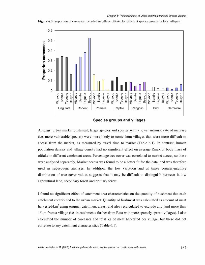
Chapter 6: The implications of urban bushmeat markets for rural villages
Allebone-Webb, S.M. (2009) Evaluating dependence on wildlife products in rural Equatorial Guinea 167
Figure 6.3 Proportion of carcasses recorded in village offtake for different species groups in four villages.
0
0.1
0.2
0.3
0.4
0.5
0.6
Mid
yobo
Sen
dje
Tegu
ete
Bea
yop
Mid
yobo
Sen
dje
Tegu
ete
Bea
yop
Mid
yobo
Sen
dje
Tegu
ete
Bea
yop
Mid
yobo
Sen
dje
Tegu
ete
Bea
yop
Mid
yobo
Sen
dje
Tegu
ete
Bea
yop
Mid
yobo
Sen
dje
Tegu
ete
Bea
yop
Mid
yobo
Sen
dje
Tegu
ete
Bea
yop
Ungulate Rodent Primate Reptile Pangolin Bird Carnivore
.
Species groups and villages
Prop
orio
n ca
rcas
ses
Amongst urban market bushmeat, larger species and species with a lower intrinsic rate of increase
(i.e. more vulnerable species) were more likely to come from villages that were more difficult to
access from the market, as measured by travel time to market (Table 6.1). In contrast, human
population density and village density had no significant effect on average Rmax or body mass of
offtake in different catchment areas. Percentage tree cover was correlated to market access, so these
were analysed separately. Market access was found to be a better fit for the data, and was therefore
used in subsequent analyses. In addition, the low variation and at times counter-intuitive
distribution of tree cover values suggests that it may be difficult to distinguish between fallow
agricultural land, secondary forest and primary forest.
I found no significant effect of catchment area characteristics on the quantity of bushmeat that each
catchment contributed to the urban market. Quantity of bushmeat was calculated as amount of meat
harvested/km2 using original catchment areas, and also recalculated to exclude any land more than
15km from a village (i.e. in catchments further from Bata with more sparsely spread villages). I also
calculated the number of carcasses and total kg of meat harvested per village, but these did not
correlate to any catchment characteristics (Table 6.1).

Chapter 6: The implications of urban bushmeat markets for rural villages
Allebone-Webb, S.M. (2009) Evaluating dependence on wildlife products in rural Equatorial Guinea 168
Table 6.1. Linear model results for the effect of catchment area characteristics on prey species profile and bushmeat total offtake. Data from 2005 only are used, to avoid effects of differential sampling of villages.
Prey profile of catchment Catchment explanatory variables (data range in brackets)
Average carcass mass
Average carcass Rmax
Kg meat/ km2
No. carcasses / km2
Average kg meat /village
Average no. carcasses/ village
Village/Km2
(0.008 - 0.09) ns
ns ns
ns ns ns
Population density (2.13 � 76.64)
ns ns ns
ns ns ns
Hrs travel (0.55 � 7.03)
(p = 0.061)
SE = 0.02 estimate = -0.058 p < 0.01
ns
ns (p = 0.07) ns
Tree Cover (63.5 � 76.8)
ns ns ns ns ns (p = 0.07)
Overall model Null model
Adj R2 = 0.33 d.f. = 15, Residual SE = 0.70
Null model
Null model
Null model
Null model
N (catchments) = 17, N (carcasses) = 12999
6.4.3 The reliability of bushmeat market data as an indicator of village
bushmeat offtake
The species profile of village bushmeat harvests was significantly different to the species profile of
carcasses reported as being sold (in village surveys), and different to the species profiles of
carcasses going from that village to the urban market, showing that some filtering processes are
taking place (Figure 6.4). For Beayop, Teguete and Sendje, hunter surveys recorded what the hunter
did with each carcass captured, showing whether it was sold (both to urban traders and local
consumers and traders) or consumed, with species over 2kg being generally more likely to be sold
than smaller species. This was lower than the average carcass mass sold to urban markets in these
villages, suggesting that the trade filters are either different or more relaxed for village sales.

Chapter 6: The implications of urban bushmeat markets for rural villages
Allebone-Webb, S.M. (2009) Evaluating dependence on wildlife products in rural Equatorial Guinea 169
The types of species more likely to be sold to urban markets varied between the two villages where
data were available. In both villages, there was a higher proportion of larger species in the urban
market sales than in the village offtake, but there were some significant differences between the two
villages. In Sendje, species with a higher price per carcass were more likely to be sold to market. In
Midyobo, by contrast, species with the highest price mark-up were more likely to be sold (Table
Figure 6.4 Graphs showing the proportion of carcasses for different weight categories in four villages.
Data are shown for all carcasses recorded in village offtake (�Village�), those carcasses reported as beingsold during village surveys to all destinations, including local sales (�Sold�), and as recorded in urbanmarket offtake during the same period. There are no urban market data for Beayop and Teguete, as these did not appear in urban markets. There are no �sold� data in Midyobo, as the destination of carcasses wasnot recorded.
0
0.1
0.2
0.3
0.4
0.5
0.6
0-2 2-4 4-7 7-12 12<
Teguete
p0
0.1
0.2
0.3
0.4
0.5
0.6
0-2 2-4 4-7 7-12 12<
Beayop
Prop
orio
n ca
rcas
ses
0
0.1
0.2
0.3
0.4
0.5
0.6
0-2 2-4 4-7 7-12 12<
Midyobo
Carcass weight categories (kg)
0
0.1
0.2
0.3
0.4
0.5
0.6
0-2 2-4 4-7 7-12 12<
Sendje
Carcass weight categories (kg)
Prop
orio
n ca
rcas
ses
VillageSoldUrban market

Chapter 6: The implications of urban bushmeat markets for rural villages
Allebone-Webb, S.M. (2009) Evaluating dependence on wildlife products in rural Equatorial Guinea 170
6.2). Consumer preference, and proportion of carcasses brought back to the village fresh had no
effect on likelihood of sale to urban areas in either village.
In both villages, species normally caught by selective methods (guns or lassos) were more likely to
be sold to market than those species normally caught by unselective methods such as traps (Table
6.1). Similarly there was a significant effect of season in both villages, with carcasses more likely to
be sold in the first (Small Dry, and relatively hot) season. Carcasses were less likely to be sold to
market in the second (First Wet, also relatively hot) season, although there was some difference
between Midyobo and Sendje. Differences between seasons were tested, and all seasons were
significantly different from each other. There was also a significant interaction between species
capture method and the season caught. Particularly in the second season, but also in the third (Big
Dry, relatively cooler) season, animals caught by selective methods were more likely to be sold to
market than those caught in traps (see Figure A 9.1).
The ability of market surveys to detect trade levels of vulnerable species was assessed by looking at
the relationship between price/carcass (Sendje) or the mark-up value (Midyobo) and species
intrinsic rate of increase (Rmax), used here as an indicator of vulnerability. For the Sendje data, the
more vulnerable species generally had a higher price (often because they are bigger). However, as
some vulnerable species (particularly primates) may have a lower price/carcass than other species
of similar vulnerability (Figure A 9.2), they may be under-represented in market surveys. A
comparison of price mark-up with Rmax in the Midyobo data shows that species with a higher
mark-up (which the data show are more likely to be sold to market) are actually the more robust
species and again vulnerable groups such as primates may be under-represented in the market.
There was some level of correlation between the explanatory variables. In particular, price/carcass
was highly correlated with species mass and price/kg, which is unsurprising given that price/carcass
is a direct function of the other two variables. Consequently mass and price/kg were analysed
separately from price/carcass. Mass and price/kg were significantly correlated to the likelihood of
sale to market in Sendje, but this model was not as good a fit to the data as the price/carcass model.
Other variables were correlated, albeit not significantly (Table A 9.1 and Table A 9.2).
Eight taxa (Panthera pardus, Loxodonta africana, Synceros caffer, Aonyx congica, Conrana
goliath, Achatina spp., squirrels and potto; see Table A 9.4 for species list) were recorded in one or
both of the two villages, but not in the urban markets (or at least not as coming from the study
villages). The lack of data on price, price mark-up and consumer preference meant that these

Chapter 6: The implications of urban bushmeat markets for rural villages
Allebone-Webb, S.M. (2009) Evaluating dependence on wildlife products in rural Equatorial Guinea 171
species were excluded from the analyses. Whilst they made up only a small proportion of carcasses
and kilos of bushmeat in the village, these taxa tended to be either very large and rare (e.g. leopards
and elephants), or small and with a very low value (e.g. squirrels, frogs and snails). Table 6.2. Factors affecting likelihood of carcasses in Sendje and Midyobo villages being sold at urban markets. Data analysed in a generalised linear mixed model with a quasi-binomial error structure.
Sendje Midyobo
Levels Parameter estimate d.f χ2 p Parameter
estimate d.f χ2 p
Explanatory Variables
Intercept -13.52 -1.29
Preference Score
ns ns
Mark-up ns 0.53 1 40.8 <0.0001
Proportion of fresh carcasses
ns NA ns
Price/carcass (log)
3.32 1 37.5 <0.0001 ns
Capture Method Chance Target
1.01
1
5.17
<0.03
-1.79 1 8.61 <0.005
Season 1 Small Dry 2 First Wet 3 Big Dry 4 Second Wet
0.58 -0.39 0 -1.23
3 556
<0.0001
0 -1.17 -3.81 0.68
3 766 <0.0001
Season:Method 1 SD/Target 2 FW/Target 3 BD/Target 4 SW/Target
0.69 0.89 0 -0.05
3 35.5
<0.0001
0 2.77 4.82 -0.58
3 138 <0.0001
Overall Model Deviance =281.5 SD (species) = 1.7022, SD (residual) = 1.6667 n (species) = 23, n (observations) = 83 n (village carcasses) = 7745, n (market carcasses) = 2119 Data collection: 4/1/03 � 20/12/03
Deviance = 579.5 SD (species) = 3.3556, SD (residual) = 2.4857 n (species) = 21, n (observations) = 78 n (village carcasses) = 7473, n (market carcasses) = 2167 Data collection: 25/4/05 - 1/2/06
This is demonstrated by the fact that average carcass mass recorded in village offtake in all four
villages is lower than that recorded in urban markets from any catchment (Figure 6.5). Similarly,
average R max is higher for village offtake than that recorded in urban market data for almost all
catchments (Figure 6.6).

Chapter 6: The implications of urban bushmeat markets for rural villages
Allebone-Webb, S.M. (2009) Evaluating dependence on wildlife products in rural Equatorial Guinea 172
Figure 6.5 Average carcass mass from different catchments in 2003 and 2005, compared to village offtake
and village offtake reported sold in four villages.
0
1
2
3
4
5
6
7
8
9
10
J 20
03L
2003
G 2
003
E 2
003
D 2
003
N 2
003
A 2
003
K 2
003
P 2
003
Q 2
003
Beay
op V
illag
eTe
guet
e V
illag
eS
endj
e V
illag
eB
eayo
p S
old
Sen
dje
Sol
dM
idyo
bo V
illag
eP
200
5N
200
5E
200
5G
200
5Te
guet
e S
old
J 20
05L
2005
Sen
dje
Mar
ket
A 2
005
Q 2
005
Mid
yobo
Mar
ket
D 2
005
K 2
005
Catchment
Ave
rage
car
cass
mas
s (k
g)
Figure 6.6 Average carcass R max from different catchments in 2003 and 2005, compared to village offtake
and village offtake reported sold in four villages.
0
0.1
0.2
0.3
0.4
0.5
0.6
0.7
0.8
0.9
P 20
03K
2003
Q 2
003
A 20
03D
200
3N
200
3E
2003
G 2
003
J 20
03L
2003
A 20
05K
2005
Q 2
005
Mid
yobo
Mar
ket
G 2
005
Tegu
ete
Sold
D 2
005
Send
je M
arke
tL
2005
J 20
05E
2005
Mid
yobo
Villa
geN
200
5Te
guet
e Vi
llage
Send
je S
old
Send
je V
illage
Beay
op S
old
P 20
05Be
ayop
Villa
ge
Catchment
Ave
rage
car
cass
Rm
ax

Chapter 6: The implications of urban bushmeat markets for rural villages
Allebone-Webb, S.M. (2009) Evaluating dependence on wildlife products in rural Equatorial Guinea 173
6.4.4 Indicators of changing exploitation
There was an overall increase in average Rmax (0.496 to 0.521) and decrease in average species
mass (5.73kg to 5.13kg) between 2003 and 2005 in Central market, and a similar increase in Rmax
(0.426 to 0.482) in Mundoasi for the same years but a small increase in average mass (5.60kg to
5.73kg). However, these figures alone say nothing about sustainability as such changes could be the
result of changing areas of hunting, changes in access, change in demand, or other factors.
A comparison of average species mass and average Rmax between 2003 and 2005 for those
catchment areas where there were >20 carcasses recorded in both years (only 9 catchments),
showed no significant difference between 2003 and 2005 (paired t-tests: mass: d.f. = 8, t = 1.75, p =
0.12; Rmax: d.f. = 8, t = -0.50, p = 0.63). However, there is a correlation between the change in
both average mass and average Rmax and travel time to catchment (Figure 6.7). Catchments
showing an increase in average Rmax or a decrease in average mass are significantly further away
from Bata. No other catchment characteristics are correlated. These results suggest that areas near to
the urban centre have already experienced some loss of larger and more vulnerable species, and that
consequently their average mass and Rmax figures may be more stable than those catchment areas
further away that are currently experiencing a decline in larger or more vulnerable species. This
may be particularly true of Central market where the traders are already going to the geographical
limits of the area (Figure 6.1).
For carcasses arriving at Central market, the average distance travelled per carcass was 33.5 km in
2003, and 45.9km in 2005. However, this could be due to a change in species composition, so this
was investigated by species. There was a significant increase in average distance travelled between
2003 and 2005 at the species level (paired t-test: t = -6.61, df = 19, p < 0.001; see Figure A 9.4).
Only Rmax is significantly correlated with the change in distance travelled, with animals with a
greater Rmax being more likely to increase the distance travelled between years (t = 2.38, p =
0.029, adjusted R2 = 0.197, df = 18, Figure A 9.5). This echoes the previous result, suggesting that
vulnerable species are already seen only in the furthest catchment areas, and it is the species of
medium to low vulnerability that traders are now having to travel further to obtain.

Chapter 6: The implications of urban bushmeat markets for rural villages
Allebone-Webb, S.M. (2009) Evaluating dependence on wildlife products in rural Equatorial Guinea 174
Figure 6.7. Change in average a) mass and b) Rmax for each catchment between 2003 and 2005, against catchment travel time to market. a) Change in average mass is significantly correlated to log travel time (t = -5.29, d.f. = 7, adjusted R-sq = 0.77, p < 0.01), analysed with a linear model, weighted by total number of carcasses in catchment. Change in average Rmax is significantly correlated to log travel time (t = 2.85, d.f. = 6, adjusted R2 = 0.44, p < 0.05).
6.5 Discussion
The data presented show that the trade filters affecting the proportion of each species sold from
hunters to urban markets are complex and may vary between villages, depending on remoteness and
the effective monopoly power of the trader. In Midyobo, a village where traders visit only once or
twice a week, species most likely to be traded were those with the highest mark-ups, or effectively
those with the highest profit per kg, so maximising trader profits. In contrast, in Sendje, a village
with much greater market access and several cars passing daily, the most significant factor in the
probability of a species being sold to urban markets was the price/carcass, effectively profitability
to hunter. A similar result has been shown by Brooks (2008), where mark-up varied with distance
for water snake traders. In both study villages, although meat was only very rarely refused by a
trader (with the exception of rotten meat), in situations where a hunter wants to sell only part of his
catch and eat the rest, the decision over which species is sold may depend on the balance of power
between the hunter and the trader.
There may also be some implications of this for selective hunting methods. Species normally
captured by a targeting method such as a gun are far more likely to be sold to market. This is
b)a)
Chapter 6: The implications of urban bushmeat markets for rural villages
Allebone-Webb, S.M. (2009) Evaluating dependence on wildlife products in rural Equatorial Guinea 175
probably due the fact that a gun hunter is more actively choosing the species hunted (and so is
unlikely to target something undesirable) and can choose the time of day or week to go hunting, and
so can coordinate hunting trips with trader visits, leaving less time for the meat to go rotten (or
avoiding having to smoke it to preserve it). Rotten meat was rarely seen in the urban markets and
smoked meat was a lower price/carcass than fresh meat, so rendering less profit per carcass.
Seasonal differences are likely to be due to a range of factors. Increased humidity and temperature
affects the ability to store bushmeat and the speed at which it rots in a trap, so meat in hot or wet
seasons (particularly if trapped) may be less likely to be fresh when the traders arrive. Other factors
also potentially affecting seasonal patterns of trade include local changes in job availability and
seasonal changes in hunter effort (e.g. more people hunting before Christmas). In addition, the
relatively small number of traders means that the decision of one individual trader to trade in a
particular week had a large effect on the data in some circumstances, which may also have
contributed to the differences between seasons.
The results suggest that market data can be a useful reflection of hunter offtake, but that to have
confidence in the results and their limitations, it is also necessary to have an understanding of the
factors affecting trade filters and consequently what may be over- or under-represented in the data.
Particular caution should be taken in assertions concerning the following taxa:
• Taxa which are vulnerable but have a relatively low market price or profit may be under-
represented in urban markets, but village offtake may still be high. In the study area,
primates are not particularly preferred, and given their high vulnerability relative to other
taxa, the overall price/carcass is therefore likely to be low compared to their vulnerability.
• Valuable or preferred species, which may be over-represented at the urban market level.
• Species which have specialist markets, are illegal to hunt or are particularly rare may not
appear in urban markets at all. In this study, some of the largest and more vulnerable
species (such as elephants, gorillas, leopards, buffalo) did not appear in the market, despite
the fact that they were recorded as being hunted in the study villages. Elephants (the only
species which require a licence to kill) were generally consumed and sold in the villages,
mainly due to problems of transporting the meat and low price/kg. Buffalo, although not
illegal to hunt, were also generally eaten and sold in the villages due to transportation
problems. The two leopards caught were consumed and sold locally, with the skin prepared
for later sale.
Unsurprisingly, species profile varies between catchment areas. However the only catchment
characteristic that affects species profile is access to the village: human population density and

Chapter 6: The implications of urban bushmeat markets for rural villages
Allebone-Webb, S.M. (2009) Evaluating dependence on wildlife products in rural Equatorial Guinea 176
vegetation cover have no significant impact. This suggests that hunting is driven more by urban
demand than local consumption and emphasises the impact of new roads and the opening of forest
areas by logging and road companies, as noted by other authors (Wilkie et al. 2000). In addition,
while I would expect a gradient of resource exploitation moving away from populated or urban
areas, our results suggest that we should base our expectations on transport and access routes, rather
than population density, forest cover, or absolute distance. The lack of attributable variation in
quantity of bushmeat between catchment areas could mean that traders are acting economically
rationally and balancing the increased costs of further transport with the ease of access albeit lower
returns of nearby areas.
Whilst it is difficult to assess the sustainability of bushmeat hunting with certainty with data
spanning only three years, our results do show changes in the species profile in Río Muni, which are
consistent with unsustainable hunting. This includes lower numbers of some species within
particular catchments, causing traders to travel further on average to buy even small, more robust
species. Traders in Central market now travel to the country border and so may have reached the
edge of the exploitation range, and therefore current changes seem to reflect an intensification of
harvesting within the existing exploitation range. Particularly, small and medium-sized species are
increasing their representation in catchment areas that are further away. The lack of village origin
data from Mundoasi in 2003 mean that the second market could not be fully analysed, but it seems
likely that traders in that market will continue to expand the frontiers towards the interior of the
country.
Data suggest that the group of species experiencing the greatest change in origin could be an
indicator of the stage of exploitation within a market. For example, in a �new� market, we might
expect large, vulnerable species to show the greatest change in average distance travelled over time
(i.e. that traders travel to buy them), as they are rapidly hunted out of nearby catchment areas. As a
market begins to mature, species of medium vulnerability may also show signs of over-exploitation
in nearby catchment areas, and so may then show greatest changes in average distance travelled. If
hunting continues to be unsustainable, we would finally expect even robust species to disappear
from catchment areas near to the market, and so over time, they too would finally show a larger
change in the average distance travelled. These results are perhaps unsurprising given the huge
increase in urban wealth and reported commercialisation of the bushmeat trade in Equatoriual
Guinea, but certainly give serious cause for concern.

Chapter 6: The implications of urban bushmeat markets for rural villages
Allebone-Webb, S.M. (2009) Evaluating dependence on wildlife products in rural Equatorial Guinea 177
These results provide a methodological defence for the use of market data as an indicator of hunter
sustainability, but with important qualifiers. They also add to mounting evidence that access of
hunters to markets is one of the most important factors affecting bushmeat harvest, and provide
cautious indicators that bushmeat hunting in continental Equatorial Guinea is having a discernable
effect on prey species profiles and wildlife populations.

Chapter 7.
Discussion

Chapter 7: Discussion
Allebone-Webb, S.M. (2009) Evaluating dependence on wildlife products in rural Equatorial Guinea 179
7.1 Dependence on wildlife in Equatorial Guinea and the
future of wildlife use
In order to answer the central question of this thesis, namely whether or not people depend on
wildlife in Equatorial Guinea, I address each of my initial research questions in turn. Then I review
potential options for management strategies, and comment on their prospects for success in
Equatorial Guinea, and finally discuss implications for future research.
7.1.1 How important are wild foods for regular use?
Households in both villages ate wild foods frequently, and gained a substantial proportion of their
diet, livelihood production and income from wild foods on a regular basis. These contributions were
particularly important given a lack of alternative food and livelihoods in either village, and
particularly in Teguete, the more remote village. The almost total absence of reared domestic meat
consumption and the low wild fish harvests meant that bushmeat provided the one animal protein
source that households could produce themselves. Even those with the financial capacity to buy
imported meat or fish were limited in choice � only smoked fish was commonly available in
Teguete, and smoked fish and frozen products in Beayop, both of which research has shown are the
least preferred meat and fish types (East et al. 2005; Kümpel 2006). The very large numbers of
women cultivating fields (almost equal to the number of households in the village) and men with
traps (almost equal to the number of households in Teguete, and approximately one third in
Beayop), and the presence of only about five paid jobs in either village attest to the low number of
livelihood options in either community. Trade provides an important income source in Beayop, but
without passing traffic in Teguete, people�s income sources are limited, and so wildlife is an
important regular (and often the only) income source for many people.
7.1.2 How important are wild foods as a safety net?
Anecdotal evidence collected during group discussions showed that some households consciously
think of the forest as a back-up plan � something to turn to when there is no food or money, and
when family cannot provide any support (chapter 5). The use of family ties and a social network as
a �community buffer� has been observed in other studies (Beuchelt et al. 2005), and evidence here
shows that this is certainly the case in Beayop and Teguete. Poorer households in Teguete
consumed more food received as a gift than in Beayop and respondents reported that family
members are the first port of call in times of need. Previous studies have pointed to wildlife being
particularly important as a buffer when social ties are broken, such as during conflict (Jamiya et al.

Chapter 7: Discussion
Allebone-Webb, S.M. (2009) Evaluating dependence on wildlife products in rural Equatorial Guinea 180
2007) or disease epidemics (Barany et al. 2004). These studies imply that social resources may be a
primary safety net, and that natural resources offer a secondary safety net, used once social
resources are exhausted or as a longer term strategy (i.e. amongst the chronically poor).
Given this, we would expect to see more evidence of forest resource use as a safety net during times
when the whole community is equally suffering resource shortages (such as during seasonal
shortages) than we would when an individual household is experiencing short-term food or income
shortages. In Río Muni, the second season was identified as the most vulnerable, probably due to
lower agricultural production, leading to lower agricultural consumption and income, and lower
total production and income, during this time. This is strong evidence that agriculture is still the
primary livelihood activity for many households, which is particularly likely given the female-
biased demographics of the villages and the gender divides in livelihood activities. Although poorer
households gained similar proportions of production and income from agriculture as wealthier
households (although lower total amounts), they were less able to make up any deficits in
production and income during the agricultural lean season, because they were less likely to earn
income from paid work or trade. During this season, households in Teguete consumed higher
average amounts of wild foods harvested directly from the forest. Bushmeat harvest contribution is
lowest in this season, and the difference is mainly made up by increased wild plant consumption,
giving strong evidence that wild plants are particularly important as a dietary safety net in Teguete
during the lean season. There was no such evidence in Beayop, the more market-integrated village.
7.1.3 Are wild foods more important for vulnerable people?
Previous studies have noted that food coping mechanisms, and �famine� behaviours may be
incorporated into the regular food and livelihood strategies of households that remain food insecure
over long periods of time (Devereux et al. 2004). If wildlife products are important as a safety net
during periods of temporarily reduced productivity such as the lean season, we would also expect
chronically poor, vulnerable people to use wildlife products more often, even as part of their regular
dietary and livelihood resources. Three such groups have been identified in this study: women,
poorer and less food secure households, and less accessible communities.
Women
Within communities and households, women produced and earned less on average, as did female-
headed households, and this is a common pattern across much of the developing world (UNDP
1995). Women are considered more vulnerable to income shocks (Khan 2001), and at the same
time, often contribute more to the welfare of the household, particularly dependents (FAO 2001).

Chapter 7: Discussion
Allebone-Webb, S.M. (2009) Evaluating dependence on wildlife products in rural Equatorial Guinea 181
Overall, there was no difference in consumption (although we might not have detected it if there
were), but men in general produced more and earned more from wildlife. However, women were
significantly more likely to use wildlife resources, which suggests that low value products are
harvested more often by women, and are therefore more likely to make up a regular contribution to
the household. Of wildlife products, women did produce substantially more wild plants. The lack of
significant sex difference in sales of wild plants implies that these small regular wildlife harvests
may be mainly consumed in the household.
Poorer and less food secure households
The most vulnerable households in both villages (as indicated by wealth or food security estimates)
produced and earned more from forest products both in absolute amounts, and as a proportion of
production and income, compared to wealthier households in the same village. This pattern was
mainly the result of bushmeat hunting. Although wealthier hunters earned higher average incomes
from hunting, bushmeat contributed most to poorer people. In addition, the poorest households
produced significantly more wild plants (but not income from wild plants) in Beayop, and the poor
in both villages were most likely to sell wildlife.
These vulnerable households were also less livelihood secure, having fewer production and income
sources, implying that the livelihoods that they did have (such as the forest) are more important
when returns from other livelihoods in their relatively smaller arsenal of livelihood options
decrease, as well as playing a proportionally more important role in regular production.
Households in the two lowest wealth ranks were also more likely to consume food produced
directly by the household, and less likely to consume imported protein, implying that for the poorest
households, alternative bought, protein-rich foods (such as domestic meat and fish) are less
accessible, probably due to the higher cost. In addition, poorer households gained a greater
proportion of protein from agricultural products, suggesting that plant proteins make up a larger
proportion of the diet. These observations were usually strongest from the second lowest wealth
rank, while the lowest wealth rank and the least food secure (especially in Teguete) relied heavily
on gifts of food, reflecting the generally low labour availability (and correspondingly low
production capacity) of these households.

Chapter 7: Discussion
Allebone-Webb, S.M. (2009) Evaluating dependence on wildlife products in rural Equatorial Guinea 182
Less accessible communities
Teguete has less access to urban centres and passing traffic than Beayop, and probably as a result its
inhabitants consumed, produced and earned less, and were less food secure. People in Teguete
relied more on wildlife for consumption, livelihood production and most particularly income. There
was a pattern between villages, whereby among poorer households, wildlife played a greater role in
income provisioning in Teguete, and a greater role in production in Beayop. This probably reflects
the lower availability of income sources and the lower actual income from those sources in Teguete.
7.1.4 How useful are urban market data as a tool for monitoring
wildlife offtake such as bushmeat?
Urban bushmeat market data were shown to be a useful tool for bushmeat monitoring, reflecting
village offtake fairly well, although vulnerable taxa with relatively low prices for their body size
such as primates may be under-represented at the market level. This should be taken into
consideration when evaluating market data on the basis of the proportions of different taxa (i.e the
proportion of primates to rodents, as reported by Wilkie & Carpenter 1999). My finding that the
bushmeat species profile differs significantly between catchment area, particularly with access to
markets, emphasises the importance of collecting data on the origin of carcasses, as notably
demonstrated by Milner-Gulland & Clayton (2002). This ensures that changes in the source of
bushmeat species, such as increased access due to new roads, traders travelling further distances, or
reduced access along certain roads, are taken into account when considering changes in species
profile over time.
There may be a large number of villages in any region, and specifically in Río Muni, whose offtake
is not reported in urban markets and so are not reflected in any assessments based on urban markets.
Considering the reduction in average animal size with market access, we would expect villages such
as Beayop (which is accessible to markets and has no protected forest area nearby) to have a
bushmeat species profile consisting of smaller, less profitable species. However, even in this
village, bushmeat represents a large percentage of income and consumption, suggesting that offtake
is still quite high. Furthermore, very few carcasses from Teguete, which does have reasonable forest
access, were recorded at the urban markets. Yet over a third of all income in Teguete comes from
bushmeat, so village offtake is likely to be substantial.
Urban market data may be a similarly useful tool to assess the harvest of other wildlife products
such as forest plants or fish, should those products become widely traded in urban areas, and given
similar assessments as to any trade filters in place. However, currently most wild plant and fish
Chapter 7: Discussion
Allebone-Webb, S.M. (2009) Evaluating dependence on wildlife products in rural Equatorial Guinea 183
products in the study villages were consumed or traded locally, so monitoring the sustainability of
harvest would have to be done at local levels.
7.1.5 What are the implications of current wildlife harvests for
continental Equatorial Guinea?
The bushmeat market data analysed here, together with previous studies (Fa et al. 1995), strongly
suggest that bushmeat hunting is unsustainable in Río Muni, at least in one urban market. Hunting
of vulnerable primates such as the black colobus may be particularly unsustainable (Kümpel 2006)
and our findings suggest that village offtake of primates may be relatively higher in rural villages
than expected from market data. The recent ban on gun-hunting in Equatorial Guinea (legislation in
2007), and the enforcement of this ban, is the first and vital step in reducing primate offtake. The
vast majority of primates are killed by gun, and given that there are few gun-hunters in either study
village, coming from wealthier households, they are less likely to depend on bushmeat as a safety-
net resource and so there will be fewer repercussions for development.
Among the remaining hunters, it does seem that wildlife harvest is important for livelihoods. That
most trade in bushmeat is done along roads is likely to be true for other products, including other
forest products. If this is the case, it makes sense that:
• Households in villages that have the most access to markets but still have good access to forests
(i.e. are near protected areas, such as Sendje), will make the most money out of wildlife.
• Households in villages that have the most access to markets, but no access to forests will
generally gain the least from the forest. Such households will probably have access to more
alternative livelihoods, including income from agriculture, but the poorest may find it especially
hard to cope. This is representative of villages near to urban areas, or peri-urban households,
and it is these households which often benefit from the nutritional and livelihood benefits from
wild plants (e.g. Gockowski et al (2003); Stoian (2005)).
• Households in villages that have the least access to markets and most access to forests will
make less money out of the trade, but there will be fewer wealth differences within the
community, and the poorest will not be so badly off (e.g. households in Teguete and Midyobo).
• Households in villages that have the least access to markets and the least access to forests will
be most vulnerable and most livelihood and food insecure (e.g. households in the North-East of
Río Muni).
Consequently, we would expect villages in the north-eastern region in Río Muni, where forest is
highly degraded, population density is high, and villages off the main roads do not have regular

Chapter 7: Discussion
Allebone-Webb, S.M. (2009) Evaluating dependence on wildlife products in rural Equatorial Guinea 184
passing traffic (and so have little access to urban areas) to be most vulnerable to food insecurity and
poverty.
7.1.6 Other issues
Comparing bushmeat, wild fish and forest plants
Bushmeat played the biggest role for livelihoods and consumption overall, and contrary to previous
studies (e.g. de Merode et al. 2004) this was still important for poorer households. However, wild
plants may contribute more to food and livelihood security in Teguete, with greater consumption in
the lean season, and greater importance to vulnerable groups such as women. Wild fish contributed
only small amounts to food and livelihoods, although this is likely to be more important in villages
near better water sources.
Demographic composition of rural areas
Teguete in particular showed a skewed demography, whereby the population was increasingly made
up of children and elderly people, and with substantially more women than men. Many households
consisted of grandparents and grandchildren (under the age of about 14) while medium-aged adults
lived and worked in urban areas, sending remittances to their rural families. One consequence of
this may be a lower number of hunters in the villages, but it is also these groups who are most likely
to be food insecure. In addition, this demographic (older people and women) are more likely to
harvest forest plants. Some have commented that this arrangement � a largely economically inactive
rural population relying heavily on presents from urban family members and imported foods � is the
best thing for conservation, given that it reduces hunter numbers. However, this is not conducive to
long-term economic development. In addition, while this may work to some extent in Equatorial
Guinea due to oil revenues and associated increases in urban wealth, it is not a model that can be
readily applied as a solution to rural poverty to other countries.
7.2 Management options
The results presented here show that in Equatorial Guinea, the poorest households have few
livelihood strategies and relatively high levels of food insecurity. In addition, commercial bushmeat
hunting, which provides a substantial portion of livelihoods, particularly among the poor, is highly
likely to be unsustainable in the longer term, which has important implications for rural
communities. The low availability of alternative protein sources in rural villages means that
bushmeat remains important for consumption, as well as income.

Chapter 7: Discussion
Allebone-Webb, S.M. (2009) Evaluating dependence on wildlife products in rural Equatorial Guinea 185
The most commonly cited solutions to reducing bushmeat hunting without negative impacts on
local communities, are the development of alternative livelihood strategies, accompanied by
disincentives to hunt, particularly commercially. There are no indications that the harvest of wild
edible fruits is unsustainable in Equatorial Guinea, and indeed these may represent an opportunity
for income generation. In contrast, the destructive harvest of products such as rattan is unlikely to
be sustainable without active management of the resource. An additional consideration is that while
it is women who are more vulnerable and contribute most to household well-being, for bushmeat
hunting disincentives to work, men must be presented with an economically attractive alternative
livelihood that is not easily combined with hunting on a regular basis. I discuss options for
alternative livelihoods and hunting disincentives below.
7.2.1 The development of alternative income-earning opportunities
Domestic meat and fish production
The production of alternative domestic meat and fish may represent an opportunity for improved
livelihoods in rural areas, proffering the combined advantages of providing income and animal
protein production. In Equatorial Guinea and other Central African countries, bushmeat is not a
preferred good, so demand may be elastic and consumers are likely to consume fresh fish and
domestic livestock alternatives if they are cheaper (East et al. 2005; Schenck et al. 2006).
Unfortunately, the domestic breeding of livestock in forested central Africa has been largely
unsuccessful. The widespread tsetse flies and trypanosomiasis severely limit cattle breeding in the
many parts of West and Central Africa, and intensive livestock rearing often involves high start-up
costs which are prohibitive for rural small holders. In addition (and if the aim is to provide
alternative livelihoods to hunting as well as alternative sources of meat), the production of livestock
often involves a different social category of people, involving wealthier entrepreneurs, as opposed
to the poor young men that commonly hunt. However, small-scale livestock rearing may be more
easily introduced. Projects have successfully introduced chicken farming in sub-Saharan Africa,
resulting in decreased bushmeat hunting or increased food security (Kitalyi 1998), and tilapia and
aquaculture projects have also been successful in Africa (Hishamunda & Ridler 2006). The
presence of one successful livestock and aquaculture farmer in Equatorial Guinea (and he is
probably the only one, INDEFOR, pers. comm.) confirms that start-up costs and knowledge are
greater barriers than external barriers such as climate and ecosystem type.
Chapter 7: Discussion
Allebone-Webb, S.M. (2009) Evaluating dependence on wildlife products in rural Equatorial Guinea 186
Increasing incomes from agriculture
In Equatorial Guinea, there may be particular potential for increased production and income from
agriculture. Agricultural production in Equatorial Guinea has significantly fallen in the last 30
years. Total agricultural production has decreased by half since the late 1960s and per capita
production has reduced by two thirds (FAO 2002), making it much lower than in neighbouring
Cameroon (FAOSTAT 2002). This has led to Equatorial Guinea being a net importer of food, even
for agricultural products and fruits such as pineapples and mangoes, which are commonly imported
from Cameroon for sale in Bata, despite being grown throughout Río Muni (pers. obs.). Although
agriculture is currently dominated by women, in the days of Spanish colonialism men cultivated
plantations of cocoa, coffee and fruits such as pineapples, and older men who remember these days
claim to prefer agricultural livelihoods than hunting as they can �sleep in the village� and not suffer
the uncomfortable realities of forest life.
Sustainable livelihoods from forest products
Wild plants
The production and marketing of forest plant food products may hold potential for improving
income in rural areas. Although wild plants have been viewed as inferior foods in some areas,
certain species may have the potential to be surprisingly profitable. Research at the International
Centre for Research in Agroforestry (ICRAF) has suggested that a number of trees in both Africa
and South America are not only important for local nutritional needs but can also play a role in food
security and in alleviating poverty in some countries (Leakey & Tchoundjeu 2001). These so called
�Cinderella� trees have been over-looked by scientists and occasionally even by local farmers, but
are now getting more attention, and several relevant species have been selected for domestication,
in the hope of expanding local and international markets (Leakey et al. 2003). Two such species in
West and Central Africa, both present in Equatorial Guinea, have been identified as important.
These are the bush mango, Irvingia gabonensis, and the African plum, Dacryodes edulis. The
former is widely eaten both for its fruit, and also for its kernel which is made into a popular sauce to
accompany many dishes. The latter is cooked and women value it for providing a quick
accompaniment to cassava. In Equatorial Guinea they are widely harvested, but not �farmed� or
traded to any great extent. However, farmers in Cameroon intercrop these species with cocoa and
coffee, using them to generate income when market commodity prices are low. This isn�t a new
strategy and the current African plum and bush mango trees found in relative abundance around
some villages in Rio Muni (compared to deep within the forest) may be a legacy of forgotten
Spanish plantations. In Cameroon in 1999, the African Plum national market was worth more than

Chapter 7: Discussion
Allebone-Webb, S.M. (2009) Evaluating dependence on wildlife products in rural Equatorial Guinea 187
$7 million, and research has shown that encouragingly, over 75% of the profits go back to the
farmers. The international market is being investigated, and there may be potential markets in
European cities with many West African immigrants. However, some have criticised the fact that
despite increasing recognition of the socio-economic importance of NTFPs, and their potential to be
over-harvested, most regions still lack sustainable management strategies for these products
(Bikoue & Essomba 2007).
Fish
In certain cases, the controlled management of fisheries and fish stocks, particularly through
community-based management, has played a significant role in increasing income and food security
(Béné et al. 2003; Dugan et al. 2006). However, the scope for increasing fish harvests and income
in Equatorial Guinea is largely unknown, and based on the low fish harvests in this study, is
unlikely to be high. As with all wildlife resources, there is an inherent limit to the number of fresh-
water fish that can be sustainably harvested, and for much of Rio Muni there are probably
insufficient rivers or access to those rivers to support many people.
Forest animals
Despite the low productivity of tropical forest mammals, and the strong evidence for unsustainable
harvest rates, bushmeat has been proposed to be useful for economic development, and there is
historical evidence that bushmeat can play a secondary role in supporting economic change.
Bushmeat played a part in underwriting the development of the Ghana cocoa industry and opening
up the forest frontier (Asibey (1974), but see Oates, 1998). However, this is unlikely to provide
enough income or be acceptable to conservationists in Equatorial Guinea, and the consensus is that
bushmeat hunting is unlikely to play a large part in rural transformation (Brown & Williams 2003).
In contrast, forest invertebrates such as wild snails and insects are gathered or reared and traded in
some parts of Africa, as �mini-livestock� (Hardouin 1997), providing regular income. In Equatorial
Guinea, forest snails are occasionally eaten and sold, particularly in villages near urban areas, and
although incomes are currently unlikely to rival incomes from bushmeat in villages beyond peri-
urban areas of high human population density, it has potential to generate income and food in the
future, especially if bushmeat hunting is severely reduced.
7.2.2 Disincentives for commercial bushmeat hunting
Some alternative livelihood projects have failed to reduce unsustainable use of natural resource, as
local communities have often, quite rationally, viewed alternative income-earning initiatives as

Chapter 7: Discussion
Allebone-Webb, S.M. (2009) Evaluating dependence on wildlife products in rural Equatorial Guinea 188
supplementary to hunting, and have continued to gain income from bushmeat as well as newly
introduced livelihoods. Consequently, there is a need to introduce disincentives for commercial
hunting at the same time as launching alternative livelihood options. In addition, new income-
earning opportunities have often failed to enlist the support of communities towards more
sustainable resource use practices, and may even have often shifted attention away from the search
for models for direct resource management.
Increase the availability and decrease the price of bushmeat substitutes
If there are no animal protein substitutes to bushmeat, attempts to decrease availability and increase
the price of bushmeat are likely to actually increase the incentives to hunt (given that forests are an
open-access resource). Thus it is crucial to increase markets for non-wild sources of animal protein
(Wilkie & Carpenter 1999). In addition to the increased production of domestic livestock and
aquaculture discussed above, the domestic breeding of forest species has often been suggested as a
potentially more successful alternative to livestock breeding. Some projects have shown that
smaller bushmeat species such as marsh cane rats (Thryonomys swinderianus), giant pouched rats
(Cricetomys emini), and brush-tailed porcupines (Atherus africanus) can be reared domestically
(Asibey 1974; Tewe & Ajaji 1982; Jori et al. 1995; Jori & Noel 1996; Jori et al. 1998; Edderai et al.
2001), but rearing these species as an alternative to hunting bushmeat will only be an attractive
option once the costs of rearing are lower than the costs of hunting. This is unlikely to be the case
until wild populations are very low, and so is not something that should be considered in Equatorial
Guinea.
Increasing the price of bushmeat relative to substitutes
If bushmeat demand is elastic (as we suspect it is in Río Muni) then an increased supply of
bushmeat substitutes should be coupled with measures to increase bushmeat price (e.g. through
fines) or reduce bushmeat supply (e.g. by limiting access to forests or enforcing offtake quotas), and
so make domestic meat options relatively cheaper, thereby reducing demand for bushmeat. To
emphasize the point, given the large reliance on bushmeat for consumption and the current lack of
alternatives in Equatorial Guinea, these measures are not appropriate without an accompanying
increase in the supply of bushmeat substitutes.
Controlling market supply
Controlling bushmeat supply to urban markets directly is a practical and relatively cheap approach
to reducing bushmeat consumption. Efforts can be concentrated on a small number of market
Chapter 7: Discussion
Allebone-Webb, S.M. (2009) Evaluating dependence on wildlife products in rural Equatorial Guinea 189
traders and enforcement need only consist of road blocks or market raids, with bushmeat being
confiscated and sellers fined, making it relatively cost effective. This also requires trustworthy law
enforcers and runs the risk of sending the bushmeat trade underground. An alternative enforcement
of market supply is to charge a market tax. This increases the effective price of bushmeat, without
encouraging corruption (except for market guards) and removes the temptation to sell confiscated
game. Even if guards do pocket taxes, the price of bushmeat will increase, and so the demand for
bushmeat and the price that traders are willing to pay hunters will fall, which should decrease
hunter incentives. However, it is unlikely that this would be enforceable outside of large urban areas
and so sales would continue within rural areas, as illustrated by the relatively low level of sales to
urban market from the study villages Teguete and Beayop.
Changing consumer preferences
Although there is no definitive preference for bushmeat in Equatorial Guinea, consumers do prefer
bushmeat in other countries (Bakarr et al. 2001). However, consumers are sometimes willing to
change their preferences for luxury goods such as ivory (O'Connell & Sutton 1990) or goods that
have little contribution to diet or household income (e.g. great apes) in response to social marketing
and education. Only when the good is necessary for a particular need, or there is no substitute
available, is changing consumer preference unlikely to be successful (Freese 1997; Fa et al. 2002).
7.2.3 Enforce sustainable hunting measures
An additional solution to reducing bushmeat harvest, and potentially increasing the likelihood that
the resource will be have the potential to act as a consumption buffer in times of real need, is to
enforce sustainable hunting measures as the same time as introducing alternative livelihood options.
Although it is likely that some species, such as most primates, have very low sustainable harvest
levels, other species, such as most rodent species, seem to maintain stable populations at far higher
levels of hunting. If trade, sales or capture of more vulnerable species (depending on the point of
enforcement) could be made illegal, while allowing trade in more robust species to continue,
hunting may be more sustainable (Kümpel et al. 2007) and the first step in this (the banning of gun-
hunting) has already occurred in Equatorial Guinea. Unfortunately, the non-selective trapping
methods used by the vast majority of hunters across Africa would make bans on particular non-
primate species difficult. Other suggestions to enforce sustainable bushmeat hunting include
working with forest industries, such as logging companies, to ensure that companies take
responsibility for bushmeat harvest within logging concessions (Schulte-Herbruggen & Davies
2006). Controlling access to who can hunt, or to hunting zones, through community management
has also been cited as a way to conserve hunted species in developing countries (Kiss 1990; Hannah

Chapter 7: Discussion
Allebone-Webb, S.M. (2009) Evaluating dependence on wildlife products in rural Equatorial Guinea 190
1992; Wells et al. 1992; Bissonette & Krausman 1995), but this requires effective community
institutions and an ability to overcome poverty�s �have-to-eat today� principle (Bodmer 1994).
Broader institutional contexts, such as informal social networks and decentralised government
structures with poor resources, may also pose a challenge to sustainable bushmeat management
(Hurst 2007).
7.3 Implications and directions for future research
This research suggests that it is important to differentiate between wealth groups and seasons when
analysing the use of wildlife products if a link to dependence is to be proven. Patterns of resource
use among vulnerable people and at vulnerable times are most reflective of a real contribution to
food and livelihood security. In addition, the higher overall contribution of wildlife to the income of
poorer wealth groups, despite higher average earnings from wildlife per person among wealthy
resource users, illustrates that it is not enough to look only at the average income gained per person
� an assessment of the total contribution to a particular group must also be considered.
During this study I measured three different indicators of wealth (income, value of fixed assets, and
wealth rank). Income and wealth rank were far better predictors of livelihood and consumption
variables, while the value of fixed assets was not widely representative of resource use or other
household variable indicators. Thus, I suggest that income and wealth rank are more useful
indicators than assets in this study system. In addition, information on income was only useful when
remittances were also considered as some relatively wealthy households earned very little income
themselves, but gained large or regular amounts of cash from family members.
Assessment of the frequency of use of food coping mechanisms was a useful tool to identify the
most vulnerable members of the community, although the results did not differ significantly from
other wealth indicators such as wealth rank. The similarity of coping strategies between two quite
different villages means that once strategies are identified, the same set of questions could be used
in other communities in the same region, negating the need for lengthy group discussions in every
survey village, and so reducing the costs and increasing the usefulness of coping strategy surveys as
a tool. However, the importance of initial extensive group discussions cannot be over-emphasised.
The first round of food security indicator data collected in 2005 suffered from an inadequate
exploration of the coping strategies proposed, resulting in some strategies that were not used in data
analysis (i.e. those differentiating between borrowing meat and fish, and separately borrowing
�other food�). In addition, distinctions that later became clear were not initially apparent, and this
resulted in lost opportunities for using strategies that may have been illuminating. In particular, in

Chapter 7: Discussion
Allebone-Webb, S.M. (2009) Evaluating dependence on wildlife products in rural Equatorial Guinea 191
grouping the consumption of all meat and fish types, I ignored the very different status attributed to
smoked fish, compared to fresh or frozen meat and fish types. Similarly, measures to identify lean
seasons need not be resource intensive. Analysis of child anthropometric data simply confirmed
what participatory discussions had identified as the hungry season, so researchers should have
confidence in the assertions of resource users.
These data illustrate that low-value products such as forest plant foods can be very important to
food security, particularly in vulnerable seasons, and yet barely register on any analysis of
economic transactions even at the village level. This suggests that studies assessing the importance
of wildlife products to communities should not over-look consumption data and the importance of
largely subsistence products.
This study involved intensive research on a range of indicators of dependence over 15 months in 2
villages. This enabled me to develop a detailed understanding of the contributions made by the little
products to consumption and livelihoods. The results confirm the importance of wildlife products to
vulnerable groups in lean seasons, as had been found by de Merode et al (2004) and others. The
strengths of this study are this details and the multi-dimensional approach to assessing dependence.
However, this is, in a way, also its weakness. The level of detailed data collected, and the multiple
indicators of wealth, while illuminating were also highly data intensive. The next step for research
on the relationships between people and wildlife products is therefore to assess changes in these
relationships on a broader geographical scale, using data on coping strategies, consumption, and
wildlife trade. Data such as these were also collected during my thesis in a further 11 communities
in Río Muni, and analysis of these data will permit assessment of these relationships at the level of
communities.
I also intend to analyse differences in hunting offtake between Beayop and Teguete using hunter
offtake data collected over six months in both villages. Using catch per unit effort (CPUE) indices,
this will allow me to compare relative wildlife abundances. In addition, it will allow me to assess
what affects the relative profitability of hunting (i.e. the relative effects of wildlife levels, market
access and price, and opportunity costs related to access to alternative livelihoods) and so to assess
at what stage hunting becomes so unprofitable so that people give it up.
Of the potential management options suggested above, it is likely that a combination will have the
greatest chance of reducing unsustainable wildlife harvest, while maintaining food and livelihood
security for rural populations. An evaluation of the potential profitability, cultural acceptance and

Chapter 7: Discussion
Allebone-Webb, S.M. (2009) Evaluating dependence on wildlife products in rural Equatorial Guinea 192
feasibility of alternative livelihood options such as small livestock production or aquaculture, is
vital to assess their practicability in Equatorial Guinea.
Enforcement of the gun-hunting ban in Equatorial Guinea will be key to the reduction in offtake of
the most vulnerable bushmeat species, namely primates. However, careful monitoring of other
bushmeat species is also necessary to ensure that species commonly trapped are also not hunted at
unsustainable levels.
7.4 Conclusions
This thesis demonstrates that wildlife resources can be important for food and livelihood security
and it is important to assess the proportion of food and income that wildlife products contribute to
vulnerable people and at vulnerable seasons to illustrate this dependence. In this way, foods such as
wild plants that contribute relatively little in total, but have considerable value to the poorest
households, can be identified. Methods to identify vulnerable households and seasons need not be
costly, but do rely on an understanding of the resource system, and a good relationship with
resource users.
People in rural Equatorial Guinea depend on wildlife for both food and income. Bushmeat provides
the greatest contribution, and is important to the poor, but it is wild forest plants that are particularly
important to the extremely vulnerable. However, the situation is hopeful. Equatorial Guinea is
unusual in that it has a relatively low human population density, high wildlife density and a high
GDP compared to most other African countries, and bushmeat is not a particularly preferred good.
Consequently, and with political will, it represents an ideal opportunity to put conservation and
development ideas for the management of bushmeat hunting and the development of alternative
livelihoods into practice: if they do not work here, they are unlikely to work elsewhere.

References
Allebone-Webb, S.M. (2009) Evaluating dependence on wildlife products in rural Equatorial Guinea 193
References
Adams, A. M., T. G. Evans, et al. (1997). "Socio-economic stratification by wealth ranking: is it valid?" World Development 25(7): 1165-1172. Albrechtsen, L. (2007). Studies of bushmeat trade in West Africa. Department of Zoology, University of Oxford. Albrechtsen, L., J. E. Fa, et al. (2005). "Contrasts in availability and consumption of animal protein in Bioko Island, West Africa: the role of bushmeat." Environmental Conservation 32(4): 340-348. Ambrose-Oji, B. (2003). "The contribution of NTFPs to the livelihoods of the 'forest poor': evidence from the tropical forest zone of south-west Cameroon." International Forestry Review 5(2): 106-117. Amous, S. (2000). The role of wood energy in Africa. Wood energy for tomorrow. Rome, FAO. Anadu, P. A., P. O. Elamah, et al. (1988). "The Bushmeat Trade in Southwestern Nigeria - a Case-Study." Human Ecology 16(2): 199-208. Arimond, M., L. E. Torheim, et al. (2008). Dietary diversity as a measure of women's diet quality in resource-poor areas: Results from rural Bangladesh site. Washington, DC, Food and Nutrition Technical Assistance (FANTA) Project/Acamdey for Educational Development (AED). Asibey, E. O. A. (1974). "The grasscutter, Thyronomys swinderianus, Temmick, in Ghana." Symposia of the Zoological Society of London 34: 161-170. Asibey, E. O. A. (1977). "Expected effects of land-use patterns on future supplies of bushmeat in Africa south of the Sahara." Environmental Conservation 4: 43-49. Atangana, A. R., V. Ukafor, et al. (2002). "Domestication of Irvingia gabonensis: 2. The selection of multiple traits for potential cultivars from Cameroon and Nigeria." Agroforestry Systems 55(3): 221-229. Auzel, P. and D. S. Wilkie (2000). Wildlife use in northern Congo: hunting in a commercial logging concession. Hunting for sustainability in tropical forests. J. G. Robinson and E. L. Bennett. New York, Columbia University Press. Awono, A., O. Ndoye, et al. (2002). "Production and marketing of Safou (Dacryodes edulis) in ameroon and internationally: market development issues." Forests, Trees and Livelihoods 12: 125-147. Ayuk, E. T., B. Duguma, et al. (1999). "Uses, management and economic potential of Irvingia gabonensis in the humid lowlands of Cameroon." Forest Ecology and Management 113: 1-9. Bakarr, M., G. Fonseca, et al. (2001). Hunting and bushmeat utilisation in the African Rainforest: A buleprint for conservation., Conservation International.

References
Allebone-Webb, S.M. (2009) Evaluating dependence on wildlife products in rural Equatorial Guinea 194
Balee, W. (1992). People of the fallow: a historical ecology of foraging in lowland South America. Conservation of neotropical forests. Working from traditional resource use. K. H. Redford and C. Padoch. New York, Columbia University Press. Barany, M., A. L. Hammett, et al. (2004). "Non-timber forest products in the food security and nutrition of smallholders afflicted by HIV/AIDS in sub-Saharan Africa." Forests, Trees and Livelihoods 14(1): 3-18. Bates, D. and D. Sarkar (2007). "lme4: Linear mixed-effects models using S4 classes. R package version 0.99875-1." BBC. (2008). "Country profile: Equatorial Guinea." http://news.bbc.co.uk/1/hi/world/africa/country_profiles/1023151.stm. Béné, C., K. Mindjimba, et al. (2003). "Inland fisheries, tenure systems and livelihood diversification in Africa: The case of the Yaéré floodplains in Lake Chad Basin." African Studies 62(2): 187 - 212. Bennett, E. and J. G. Robinson (2000). Hunting of wildlife in tropical forests: Implications for biodiversity and forest peoples. Washington D.C., The World Bank. Bennett, E. L. (2002). "Is there a link between wild meat and food security?" Conservation Biology 16(3): 590-592. Beuchelt, T., I. Fischer, et al. (2005). Social networks as a means of information exchange and risk-management - a case study from Northern Vietnam. Conference on International Agricultural Research for Development, Tropentag. Bhattacharya, A. K. and I. Patra (2007). "Non-timber forest products (NTFP), livelihoods and nutrition interface - A study of the tribal communities of Madhya Pradesh and Maharashtra States in India." Indian Forester 133(11): 1449-1462. Bi, I. A. Z. and K. L. Kouakou (2004). "Study of rattan production-to-consumption system in the district of Abidjan (South Cote d'Ivoire)." Biotechnologie, Agronomie, Societe et Environnement 8(3): 199-209. Bikoue, M. A. C. and H. Essomba (2007). "Management of natural resources which supply edible non-wood forest products in Central Africa." Non-Wood Forest Products Working Document(No.5): xii + 103. Biloso, A. and J. Lejoly (2006). "Study of non woody forest products exploitation and market in Kinshasa." Tropicultura 24(3): 183-188. Bird, N. and C. Dickson (2007). Bushmeat, forestry and livelihoods: exploring the coverage in Poverty Reduction Strategy Papers. Bushmeat and livelihoods: wildlife management and poverty reduction. G. Davies and D. Brown. Oxford, Blackwell Publishing. Bissonette, J. A. and P. R. Krausman (1995). Integrating people and wildlife for a sustainable future. Proceedings of the First International Wildlife Management Congress., Bethesda, MD, The Wildlife Society. Blake, S. (1994). A survey along the western border of the Nouable-Ndoki National Park, Northern Congo. Report to Noudable-Ndoki National Park management.
References
Allebone-Webb, S.M. (2009) Evaluating dependence on wildlife products in rural Equatorial Guinea 195
Bodmer, R. E. (1994). Managing wildlife with local communities in the Peruvian Amazon: The case of the Reserva Communal Tamshiyacu-Tahuayo. Natural connections: Perspectives in Community-Based Conservation. D. Western, R. M. Wright and S. C. Strum. Washington DC, Island Press: 113-134. Bowen-Jones, E. (1998). A review of the commercial bushmeat trade with emphasis on Central/West Africa and the great apes. Cambridge, The Ape Alliance/Flora Fauna International. Brashares, J. S., P. Arcese, et al. (2001). "Human demography and reserve size predict wildlife extinction in West Africa." Proceedings of the Royal Society of London Series B-Biological Sciences 268(1484): 2473-2478. Brashares, J. S., P. Arcese, et al. (2004). "Bushmeat hunting, wildlife declines, and fish supply in West Africa." Science 306: 1180-1183. Brooks, S. E. (2008). Integrating livelihoods, economics and ecology for conservation: snake exploitation in Cambodia, University of East Anglia. Brown, D. and A. Williams (2003). "The case for bushmeat as a component of development policy: issues and challenges." International Forestry Review 5(2): 148-155. Brown, L. and H. Kane (1994). Full House: Reassessing the Earth's Population Carrying Capacity. New York, Norton. Caro, T. M. (1999). "Demography and behaviour of African mammals subject to exploitation." Biological Conservation 91(1): 91-97. Cayuela Serrano, N., D. V. Joiris, et al. (2000). Guinée Equatoriale. Les peuples des forêts tropicales aujourd'hui. Volume III: Région Afrique Centrale. S. Bahuchet and P. de Maret, Avenir des Peuple des Forêts Tropicales (APFT). Chambers, R., R. Longhurst, et al. (1981). Seasonal dimensions to rural poverty. London, Frances Pinter. Chapman, C. A., A. Gautier-Hion, et al. (1999). African primate communities: determinants of structure and threats to survival. Primate communities. J. G. Fleagle, C. Janson and K. E. Reed. Cambridge, Cambridge University Press. Chardonnet, P., H. Fritz, et al. (1995). Current importance of traditional and major contrasts in wild meat consumption in Sub-Saharan Africa. Integrating People and Wildlife for a Sustainable Future. Proceedings of the first international wildlife management congress., Bethesda, MD., The Wildlife Society. Chege, N. (1994). "Africa's non-timber forest economy." World Watch 7(4): 19-24. CIA. (2008). "The World Factbook." Clayton, L., M. Keeling, et al. (1997). "Bringing home the bacon: A spatial model of wild pig hunting in Sulawesi, Indonesia." Ecological Applications 7(2): 642-652.
References
Allebone-Webb, S.M. (2009) Evaluating dependence on wildlife products in rural Equatorial Guinea 196
Coates, J., A. Swindale, et al. (2007). Household food insecurity access scale (HFIAS) for measurement of food access: Indicator guide (version 3). Washington, D.C., Food and Nutrition Tecnical Assistance Project (FANTA), Academy for Educational Development. Coates, J., P. Webb, et al. (2003). Measuring Food Insecurity: Going beyond indicators of income and anthropology. Washingotn, DC, Food and Nutrition Technical Assistance Project, Academy for Educational Development. Cogels, S. (1997). Etude terroir d'Ayamiken, CUREF. Cooperacion Sanitaria Española con Guinea Ecuatorial (1991). La alimentación y la cocina en Guinea Ecuatorial (cultivo, caza y pesca). Madrid, Ministerio de Sanidad y Consumo España. Corbett, J. (1988). "Famine and Household Coping Strategies." World Development 16(9): 1099-1112. Cowlishaw, G., S. Mendelson, et al. (2005). "Evidence for post-depletion sustainability in a mature bushmeat market." Journal of Applied Ecology 42(3): 460-468. Cowlishaw, G., S. Mendelson, et al. (2005). "Structure and operation of a bushmeat commodity chain in southwestern Ghana." Conservation Biology 19(1): 139-149. Cowlishaw, G., S. Mendelson, et al. (2007). Livelihoods and sustainability in a bushmeat commodity chain in Ghana. Bushmeat and livelihoods. G. Davies and D. Brown. Oxford, Blackwell Publishing & ZSL. Cowlishaw, G., S. Mendelson, et al. (2003). Evidence for post-depletion sustainability in a mature bushmeat chain. Draft, Zoological Society of London. Crookes, D., D. Humphreys, et al. (2007). "The role of hunting in village livelihoods in the Ashanti region, Ghana." South African Journal of Economic and Management Sciences 10(4): 457-469. Crookes, D. J., N. Ankudey, et al. (2005). "The value of a long-term bushmeat market dataset as an indicator of system dynamics." Environmental Conservation 32(4): 333-339. CUREF (2002). Carte Guinea Ecuatorial (ArcView). Bata, Guinea Ecuatorial, Proyecto de Conservación y Utilización Racional de los Ecosistemas Forestales, Ministerio de Bosques, Pesca y Medio Ambiente. Daniggelis, E. (1997). The Jangal's "hidden" buffer for household food security among marginalized farmers in Nepal. XI World Forestry Congress. Davies, G. and D. Brown (2007). Bushmeat and livelihoods: wildlife management and poverty reduction, Blackwell Publishing. de Beer, J. H. and M. L. McDermott (1996). The economic value of Non-Timber Forest Products in South East Asia. Amsterdam, Netherlands Committee for IUCN. de Foliart, G. (1992). "Insects as human food." Crop Protection 11(5): 395-399. de Foliart, G. R. (1999). "Insects as food: Why the Western attitude is important." Annual Review of Entomology 44: 21-50.

References
Allebone-Webb, S.M. (2009) Evaluating dependence on wildlife products in rural Equatorial Guinea 197
de Merode, E., K. Homewood, et al. (2004). "The value of bushmeat and other wild foods to rural households living in extreme poverty in Democratic Republic of Congo." Biological Conservation 118(5): 573-581. de Nigris, M. (1997). Urbanisation and food demand in Africa. Food into cities collection, FAO. de Onis, M., A. W. Onyango, et al. (2004). "Measurement and standardization protocols for anthropometry used in the construction of a new international growth reference, for the WHO Multicentre Growth Reference Study Group." Food and Nutrition Bulletin 25 (Supplement): S27-36 (see http://www.who.int/childgrowth/mgrs/en). de Waal, A. (1988). "Famine early warning systems and the use of socio-economic data." Disasters 12: 81-91. del Ninno, C. and P. A. Dorosh (2003). "Public policy, markets and household coping strategies in Bangladesh: Avoiding a food security crisis following the 1998 floods." World Development 31(7): 1221-1238. Delacote, P. (2007). "Agricultural expansion, forest products as safety nets, and deforestation." Environment and Development Economics 12: 235-249. Delang, C. O. (2006). "Not just minor forest products: The economic rationale for the consumption of wild food plants by subsistence farmers." Ecological Economics 59(1): 64-73. Delang, C. O. (2006). "The role of wild food plants in poverty alleviation and biodiversity conservation in tropical countries." Progress in Development Studies 6(4): 275-286. Dethier, M. (1995). Etude chasse. Yaounde, ECOFAC: 120. Devereux, S., B. Baulch, et al. (2004). Improving the analysis of food insecurity. Food insecurity measurement, livelihoods approaches and policy: Applications in FIVIMS, Prepared for the Food Insecurity and Vulnerability Information and Mapping Systems (FIVIMS) Secretariat. DFID (2002). Inland Fisheries. Key Sheets: Resource Management. J. Farrington. Dounias, E. (1993). Dynamique et gestion différentielles du système de production á dominante agricole des Mvae du sud-Cameroun forestier. Sciences et Techniques du Languedoc. Montpellier, Université Montpellier II. Dounias, E. and C. J. P. Colfer (2008). Sociocultural dimensions of diet and health in forest-dwellers' systems. Human health and forests. A global overview of issues, practice and policy. C. J. P. Colfer. London, Earthscan. Draulans, D. and E. Van Krunkelsven (2002). "The impact of war on forest areas in the Democratic Republic of Congo." Oryx 36(1): 35-40. Dugan, P., M. M. Dey, et al. (2006). "Fisheries and water productivity in tropical river basins: Enhancing food security and livelihoods by managing water for fish." Agricultural Water Management 80(1-3): 262-275. East, T., N. K. Kümpel, et al. (2005). "Determinants of urban bushmeat consumption in Rio Muni, Equatorial Guinea." Biological Conservation 126(2): 206-215.

References
Allebone-Webb, S.M. (2009) Evaluating dependence on wildlife products in rural Equatorial Guinea 198
ECOFAC. (2003). "Equatorial Guinea component Monte Alén National Park." URL http://www.ecofac.org/EN/C4-EquatorialGuinea.htm. Edderai, D., M. Ntsame, et al. (2001). "Reproduction management in cane-rats breeding. Synthesis of the existing tools and methods." Productions Animales 14(2): 97-103. Education International (2007). "Barometer of Human and Trade Union Rights in Education." Egal, F., A. Ngom, et al. (2000). "Integration of food security and nutrition in forestry planning: the role of participatory approaches." Unasylva 51(3): 19-23. Ehrlich, P. R. and A. H. Ehrlich (1990). The population explosion. New York, Simon & Schuster. Equatorial Guinea Census (2001). Population census, as reported in 'Informaciones suplementarias pedidas por el comité de derechos del niño al gobierno de Guinea Ecuatorial (CRC/C/RESP/68), Comité de los derechos del niño. Fa, J. E. (2000). Hunted animals in Bioko Island, West Africa: sustainability and future. Hunting for sustainability in tropical forests. J. Robinson and E. Bennett. Columbia, Columbia University Press: 165-195. Fa, J. E., D. Currie, et al. (2003). "Bushmeat and food security in the Congo Basin: linkages between wildlife and people's future." Environmental Conservation 30(1): 71-78. Fa, J. E., J. Juste, et al. (2002). "Bushmeat consumption and preferences of two ethnic groups in Bioko Island, West Africa." Human Ecology 30(3): 397-416. Fa, J. E., J. Juste, et al. (1995). "Impact of market hunting on mammal species in Equatorial Guinea." Conservation Biology 14: 1602-1613. Fa, J. E., S. Seymour, et al. (2006). "Getting to grips with the magnitude of exploitation: Bushmeat in the Cross-Sanaga Rivers region, Nigeria and Cameroon." Biological Conservation 129(4): 497-510. Fa, J. E. and D. Wilkie (2002). Reducing demand by developing economically acceptable alternative to wildlife meat. 16th Annual Meeting of the Society for Conservation Biology, Canterbury, UK. Fa, J. E., J. E. G. Yuste, et al. (2000). "Bushmeat markets on Bioko Island as a measure of hunting pressure." Conservation Biology 14(6): 1602-1613. Falconer, J. (1990). The major significance of minor forest products. Community Forestry Note, No. 6. Rome, Food and Agricultue Organization. FAO (1988). "Traditional Food Plants." Food and Agricultural Organisation Rome. FAO (1990). "The major significance of 'minor' forest products: the local use and value of forests in the West African humid forest zone." FAO Community Forestry Note(No. 6): x + 232. FAO (1996). Forestry policies of selected countries in Africa. Rome, Food and Agriculture Organization of the United Nations.

References
Allebone-Webb, S.M. (2009) Evaluating dependence on wildlife products in rural Equatorial Guinea 199
FAO (1997). Agriculture, food and nutrition for Africa - a resource book for teachers of agriculture, Food and Nutrition Division, Food and Agriculture Organization (FAO). FAO (2001). Gender: key to sustainability and food security, Fodo and Agriculture Organization of the United Nations. FAO (2001). The impact of HIV/AIDS on food security, Rome, Food and Agricultural Organization of the United Nations. FAO (2002). "The state of food insecurity in the world 2002." FAO. (2003). "Special programme for food security." from http://www.fao.org/spfs. FAO (2003). The state of food insecurity in the world 2003: monitoring progress towards the World Food Summit and Milllennium Development Goals. Rome, Food and Agricultural Organization of the United Nations. FAO (2004). The state of food insecurity in the world 2004. FAO (2006). Inland fisheries and rural livelihoods, FishCode-STF & Fisheries Department, FAO. FAO and WHO (1985). Energy and protein requirements. World Health Organization Technical Report 724. Geneva, Switzerland. FAO/FIVIMS (2003). Measurement and assessment of food deprivation and undernutrition. Proceedings of an international scientific symposium, Rome, 2002, Food and Agriculture Organization of the United Nations/ Food Insecurity and Vulnerability Information and Mapping System. FAOSTAT (2002). World Bank World Development Indicators. Fisher, M. (2004). "Household welfare and forest dependence in Southern Malawi." Environment and Development Economics 9: 135-154. Fleuret, A. (1979). "Methods for evaluation of the role of fruits and wild greens in Shambaa diet: a case study." Medical Anthropology 3: 249-269. Foppes, J. and R. Dechaineux (2000). Non-timber forest products in Lao PDR: a practical application of teh ecosystems approach? Presented at the Pathfinder Workshop on An Ecosystem Approach un the Convention on Biological Diversity (CBC): From concept to action, Malaysia. Foppes, J. and S. Ketphanh (1997). The use of NTFPs in Lao PDR. DoF/IUCN NTFP Project. Vientiane. Ford Foundation (1998). Forestry for sustainable rural development. A review of Ford Foundation-Supported Community Forestry Programs in Asia. New York. Freese, C. H. (1997). Harvesting wild species: Implications for biodiversity conservation. Balitmore, USA, John Hopkins University Press. Frongillo, E. A., N. Chowdhury, et al. (2003). "Understanding the experience of household food insecurity in rural Bangladesh leads to a measure different from that used in other countries." Journal of Nutrition 133(12): 4158-4162.
References
Allebone-Webb, S.M. (2009) Evaluating dependence on wildlife products in rural Equatorial Guinea 200
Future-Harvest. (2001). "With time running out scientists attempt rescue of African vegetable crops." News feature. Geist, V. (1988). "How markets in wildlife meat and parts, and the sale of hunting privelges, jeopardize wildlife conservation." Conservation Biology 2: 15-26. Gillingham, S. and P. C. Lee (2003). "People and protected areas: a study of local perceptions of wildlife crop-damage conflict in an area bordering the Selous Game Reserve, Tanzania." Oryx 37(3): 316-325. Gockowski, J., J. Mbazo'o, et al. (2003). "African traditional leafy vegetables and the urban and peri- urban poor." Food Policy 28(3): 221-235. Godoy, R., N. Brokaw, et al. (1995). "The effect of income on the extraction of non-timber tropical forest products: model, hypotheses, and preliminary findings from the Sumu Indians of Nicaragua." Human Ecology 23: 29-52. Guijt, I., F. Hinchcliffe, et al. (1995). The hidden harvest: The value of wild resources in agricultural systems. Sustainable Agriculture Programme, International Institute for Environment and Development. Haddad, L., C. Peña, et al. (1996). Food security and nutrition implications of intrahousehold bias: A review of literature. FCND Discussion Paper No. 19. Washington, D.C., IFPRI. Hall, B. (2004). Understanding food security data and methodology, Food Security Institute, Centre on Hunger and Poverty. Hannah, L. (1992). African people, African parks: An evaluationg of development initiatives as a means of improving protected area conservation in Africa. Washington, DC, Conservation International. Hansen, M., R. DeFries, et al. (2002). Global percent tree cover at spatial resolution of 500 meters: first results of the MODIS vegetation continuous fields algorithm. Hansen, M., R. DeFries, et al. (2002). "Towards an operational MODIS continuous field of percent tree cover algorithm: examples using AVHRR and MODIS data." Remote Sensing of Environment 83: 303-319. Hardouin, J. (1997). "Developing minilivestock as source of human food, animal feed or revenue: A brief overview." Ecology of Food and Nutrition 36(2-4): 95-&. Hearn, G. W. and W. A. Morra (2001). The approaching extinction of monkeys and duikers on Bioko Island, Equatorial Guinea, Africa. Glenside, USA, Arcadia University Bioko Biodiversity Protection Program. Hilton-Taylor, C. (2000). 2000 IUCN red list of threatened species. Gland, Switzerland, World Conservation Union. Hishamunda, N. and N. B. Ridler (2006). "Farming fish for profits: A small step towards food security in sub-Saharan Africa." Food Policy 31(5): 401-414. Hoskins, M. (1990). "The contribution of forestry to food security." Unasylva 41(1): 3-13.

References
Allebone-Webb, S.M. (2009) Evaluating dependence on wildlife products in rural Equatorial Guinea 201
Hoskins, M. (1990). The contribution of forestry to food security. Forestry and food security, FAO. Hurst, A. (2007). Institutional challenges to sustainable bushmeat management in Central Africa. Bushmeat and livelihoods: wildlife management and poverty reduction. G. Davies and D. Brown. Oxford, Blackwell Publishing. IFPRI (2002). Measuring and assessing food deprivation and undernutrition. Rome, International Food Policy Research Institute. Illgner, P. and E. Nel (2000). "The geography of edible insects in sub-Saharan Africa: A study of the mopane caterpillar." Geographical Journal 166: 336-351. IMF (2006). IMF Country Report No. 06/233, Equatorial Guinea, International Monetary Fund (IMF). IMF (2006). Republic of Equatorial Guinea: Selected issues and statistical appendix. IMF Country Report No. 06/237. Washington D.C., USA, International Monetary Fund. IMF (2007). World Economic Outlook Database, October 2007, International Monetary Fund (IMF). International Panel on Climate Change (2001). Climate Change 2001: Impacts, Adaptation and Vulnerability. Cambridge, Cambridge University Press. IUCN. (2003). "IUCN website." from http://www.iucn.org. Jamiya, G., s. Milledge, et al. (2007). 'Night Time Spinach': Conservation and livelihood implications of wild meat use in refugee situations in north-western Tanzania. Dar es Salaam, Tanzania, TRAFFIC East/Southern Africa. Jerozolimski, A. and C. A. Peres (2003). "Bringing home the biggest bacon: a cross-site analysis of the structure of hunter-kill profiles in Neotropical forests." Biological Conservation 111(3): 415-425. JeuneAfrique (2008). Guinée écuatoriale: le parti présidentiel grand vainquer des législatives. JeuneAfrique.com. Malabo: http://www.jeuneafrique.com/fluxafp/fil_info.asp?reg_id=0&art_cle=45593. Jimoh, S. O. and E. A. Haruna (2007). "Contributions of non-timber forest products to household food security and income around Onigambari forest reserve, Oyo State, Nigeria." Journal of Environmental Extension 6: 28-33. Jori, F., M. Lopez-Bejar, et al. (1998). "The biology and use of the African brush-tailed porcupine (Atherurus africanus, Gray, 1842) as a food animal. A review." Biodiversity and Conservation 7(11): 1417-1426. Jori, F., G. A. Mensah, et al. (1995). "Grasscutter Production - an Example of Rational Exploitation of Wildlife." Biodiversity and Conservation 4(3): 257-265. Jori, F. and J. M. Noel (1996). Guide pratigue de'levage d'autacodes au Gabon. Berthelot, Gabon, Veterinaires Sans Frontieres.

References
Allebone-Webb, S.M. (2009) Evaluating dependence on wildlife products in rural Equatorial Guinea 202
Juste, J., J. E. Fa, et al. (1995). "Market dynamics of bushmeat species in Equatorial-Guinea." Journal of Applied Ecology 32(3): 454-467. Kaimowitz, D. (2003). Not by bread alone... forests and rural livelihoods in sub-Saharan Africa. Forestry and poverty reduction strategies: capturing the potential. EFI Proceedings No. 47. T. Oksanen, B. Pajari and T. Tuomasjukka. Joensuu, European Forest Institute. Katerere, Y. (1998). "Non-timber products key in Central Africa's forest." Forum 13(1): 85-88. Khan, M. H. (2001). Rural poverty in developing countries. Implications for public policy. Economic Issues No. 26, International Monetary Fund. King, S. (1994). "Utilisation of wildlife in Bakossiland, West Cameroon with particular reference to primates." TRAFFIC bulletin 14: 63-73. Kingdon, J. (1997). The Kingdon field guide to African mammals, Academic Press. Kiss, A. (1990). Living with wildlife: Wildlife resources management with local participation in Africa. Washington, DC, World Bank: Technical paper No. 130. Kitalyi, A. J. (1998). Village chicken production systems in rural Africa. Household food security and gender issues. FAO Animal Production and Health Paper 142, FAO. Koppert, G. J. A., E. Dounias, et al. (1993). Food consumption in three forest populations of the southern coastal area of Cameroon: Yassa - Mvae - Bakola. Tropical forests, people and food. Biocultural interactions and applications to development. C. M. Hladik, A. Hladik, O. F. Linareset al. Paris, UNESCO & Carnforth: The Parthenon Publishing Group. Koppert, G. J. A., E. Dounias, et al. (1996). Consommation alimentaire dans trois populations forestières de la région côtière du Cameroun: Yassa, Mvae et Bakola. L'alimentation de forêt tropicale: interactions bioculturelles et perspectives de développement. C. M. Hladik, A. Hladik and A. Pagezy. Orstom, Paris, UNESCO: 477-496. Kümpel, N. K. (2006). Incentives for sustainable hunting of bushmeat in Río Muni, Equatorial Guinea. London, UK, PhD thesis, Imperial College London. Kümpel, N. K., T. East, et al. (2007). Determinants of bushmeat consumption and trade in continental Equatorial Guinea: an urban-rural comparison. Bushmeat and Livelihoods. G. Davies and D. Brown, Blackwell Publishing. Leakey, R. R. B., K. Schreckenberg, et al. (2003). "The participatory domestication of West African indigenous fruits." International Forestry Review 5(4): 338-347. Leakey, R. R. B. and Z. Tchoundjeu (2001). "Diversification of tree crops: Domestication of companion crops for poverty reduction and environmental services." Experimental Agriculture 37(3): 279-296. LeBreton, M., A. T. Prosser, et al. (2006). "Patterns of bushmeat hunting and perceptions of disease risk among central African communities." Animal Conservation 9(4): 357-363. Levang, P. and FPP-Bulungan team (2002). People's dependencies on forests. Technical Report, Phase 1 1997-2001. ITTO project PD 12/97 Rev.1. Forest, science and sustainability: The Bulungan Model Forest. I. T. T. O. (ITTO) and C. f. I. F. Research.

References
Allebone-Webb, S.M. (2009) Evaluating dependence on wildlife products in rural Equatorial Guinea 203
Loibooki, M., H. Hofer, et al. (2002). "Bushmeat hunting by communities adjacent to the Serengeti National Park, Tanzania: the importance of livestock ownership and alternative sources of protein and income." Environmental Conservation 29(3): 391-398. Ludwig, D., R. Hilborn, et al. (1993). "Uncertainty, resource exploitation and conservation: lessons from history." Science 260: 17 & 36. Luxmore, R. A. (1994). Impact on conservation. Wildlife production systems. Hudson et al. Cambridge. LWAG (2002). Wildlife and poverty study, Livestock and Wildlife Advisory Group (LWAG), DfID's Rural Livelihoods Department. ma Mbalele, M. (1978). "Part of African culture." Unasylva 29: 16-17. Mainka, S. and M. Trivedi (2002). Links between biodiversity conservation, livelihoods and food security: The sustainable use of wild species for meat. The IUCN Species Survival Commission, IUCN. Malaisse, F. (1997). Se nourrir en forêt claire africaine. Approche écologique et nutritionnelle. Les presses agronomiques de Gembloux, Gembloux, Belique. Malleret-King, D. (2000). A food security approach to Marine Protocol Area impacts on surrounding fishing communities: The case of Kisite Marine National Park in Kenya. Biological Sciences, Marine Resource Management, University of Warwick, UK. Marconi, S., P. Manzi, et al. (2002). "Nutritional evaluation of terrestrial invertebrates as traditional food in Amazonia." Biotropica 34(2): 73-80. Martin, G. H. G. (1983). "Bushmeat in Nigeria as a Natural-Resource with Environmental Implications." Environmental Conservation 10(2): 125-132. Martin, T. G., B. A. Wintle, et al. (2005). "Zero tolerance ecology: improving ecological inference by modelling the source of zero observations." Ecology Letters 8(11): 1235-1246. Maxwell, D., C. Ahiadeke, et al. (1999). "Alternative food-security indicators: revisiting the frequency and severity of 'coping strategies'." Food Policy 24(4): 411-429. Maxwell, D., B. Watkins, et al. (2003). The coping strategies index: a tool for rapidly measuring food security and the impact of food aid programmes in emergencies. FAO International Workshop on "Food security in complex emergencies: building policy frameworks to address longer-term programming challenges", Tivoli, Eastern and Central Africa Regional Management Unit, CARE Vulnerability Assessment and Mapping, World Food Programme. Maxwell, D. G. (1996). "Measuring food insecurity: The frequency and severity of ''coping strategies''." Food Policy 21(3): 291-303. Mialoundama, F. (1993). Nutritional and socio-economic value of Gnetum leaves in Central Africa forest. Tropical forests, people and food: Biocultural interactions and applications to development. C. M. Hladik, A. Hladik, O. F. Linareset al. Paris, UNESCO.

References
Allebone-Webb, S.M. (2009) Evaluating dependence on wildlife products in rural Equatorial Guinea 204
Milner-Gulland, E. J., E. L. Bennett, et al. (2003). "Wild meat: the bigger picture." Trends in Ecology & Evolution 18(7): 351-357. Milner-Gulland, E. J. and L. Clayton (2002). "The trade in babirusas and wild pigs in North Sulawesi, Indonesia." Ecological Economics 42(1-2): 165-183. Mlay, G., F. Turuka, et al. (2000). Agricultural sector policies and forestry development in selected countries in Southern Africa. Workshop on policies, governance and harvesting in miombo woodlands, Arusha, Tanzania. Narendran, K., I. K. Murthy, et al. (2001). "Nontimber forest product extraction, utilization and valuation: A case study from the Nilgiri Biosphere Reserve, southern India." Economic Botany 55(4): 528-538. Nasi, R., D. Brown, et al. (2008). "Conservation and use of wildlife-based resources: the bushmeat crisis." CBD Technical Series(33): 50 pp. Nasi, R. and T. Cunningham (2001). Sustainable management of non-timber forest resources: A review with recommendations for the SBSTTA. Montreal, Secretariat to the Convention on Biological Diversity. Ndoye, O. and A. Awono (2005). The markets of non-timber forest products in the provinces of Equateur and Banundu, Deomcratic Republic of Congo. Report for the Congo livelihood improvement and food security project, USAID. Yaoundé, Cameroon, Centre for International Forestry Research (CIFOR), Regional Office for Central Africa. Ndoye, O., M. R. Perez, et al. (1998). "The markets of non-timber forest products in the Humid Forest Zone of Cameroon." Network Paper - Rural Development Forestry Network(No. 22c): 20. Neumann, C., D. M. Harris, et al. (2002). "Contribution of animal source foods in improving diet quality and function in children in the developing world." Nutrition Research 22(1-2): 193-220. Neumann, R. P. and E. Hirsch (2000). Commercialisation of Non-Timber Forest Products: Review and Analysis of Resarch. Bogor, CIFOR. Ngnegueu, P. R. and R. C. Fotso (1996). Chasse villageoise et consequences pour la conservation de la biodiversite dans la reserve de biosphere du Dja. Yaounde, ECOFAC. Njiforti, H. L. (1996). "Preferences and present demand for bushmeat in north Cameroon: Some implications for wildlife conservation." Environmental Conservation 23(2): 149-155. Nkwatoh, A. F. and G. S. Yinda (2007). "Assessment of Non-Timber Forest Products (NTFPs) of economic potentials in the Korup National Park, of South West Cameroon." Global Journal of Agricultural Sciences 6(1): 41-48. Noss, A. J. (1998). "Cable snares and bushmeat markets in a central African forest." Environmental Conservation 25(3): 228-233. Ntiamoa-Baidu, Y. (1997). Wildlife and food security in Africa. FAO conservation guide No. 33. Rome, Food and Agriculture Organisation. O'Connell, M. A. and M. Sutton (1990). The effect of trade on international commerce in Africa elephant ivory. Washington, DC, World Wildlife Fund.

References
Allebone-Webb, S.M. (2009) Evaluating dependence on wildlife products in rural Equatorial Guinea 205
Oben, J. E., J. L. Ngondi, et al. (2008). "The use of a Cissus quadrangularis/Irvingia gabonensis combination in the management of weight loss: a double-blind placebo-controlled study." Lipids in Health and Disease 7. Oficina Central del Censo (1997). Resumen de los principales resultados del II Censo General de poblacion y viviendas en Guinea Ecuatorial. Malabo, Direccion General de Estadistica y Cuentas Nacionales, Ministério de Planificación y Desarrollo Económico, Republica de Guinea Ecuatorial,. Oficina Central del Censo (2002). Resumen de los principales resultados del III Censo General de poblacion y viviendas en Guinea Ecuatorial. Malabo, Direccion General de Estadistica y Cuentas Nacionales, Ministério de Planificación y Desarrollo Económico, Republica de Guinea Ecuatorial,. Ogden, C. (1990). "Building nutritional considerations into forestry development efforts." Unasylva 41(1): 20-28. Ogoye-Ndegwa, C. and J. Aagaard-Hansen (2003). "Traditional gathering of wild vegetables among the Luo of Western Kenya - A nutritional anthropology project." Ecology of Food and Nutrition 42(1): 69-89. Okafor, J. C. (1997). Conservation and use of traditional vegetables from woody forest species in south-eastern Nigeria. Traditional African Vegetables. Promoting the Conservation and Use of Under-utilized and Neglected Crops. 16. Proceedings of the IPGRI International Workshop on Genetic Resources of Traditional Vegetables in Africa: Conservation and Use, ICRAF HQ, Nairobi, Kenya, Institute of Plant Genetics and Crop Plant Research, Gatersleben/International Plant Genetics Resources Institute, Rome, Italy. Oldewage-Theron, W. H., E. G. Dicks, et al. (2006). "Poverty, household food insecurity and nutrition: Coping strategies in an informal settlement in the Vaal Triangle, South Africa." Public Health 120(9): 795-804. ORNL LandScanTM (2005). High Resolution Global Population Dataset, TM/UT-Battelle, LLC. Owusu, E. H., Y. Ntiamoa-Baidu, et al. (2006). "The dependence of local people on bushmeat in the Afadjato and Agumatsa Conservation Area, Ghana." Nature & Faune 21(1): 33-44. Pandit, B. H. and G. B. Thapa (2003). "A tragedy of non-timber forest resources in the mountain commons of Nepal." Environmental Conservation 30(3): 283-292. Park, C. S. (2006). "Risk pooling between households and risk-coping measures in developing countries: Evidence from rural Bangladesh." Economic Development and Cultural Change 54(2): 423-457. Pattanayak, S. K. and E. O. Sills (2001). "Do tropical forests provide natural insurance? The microeconomics of non-timber forest product collection in the Brazilian Amazon." Land Economics 77(4): 595-613. Pedersen, J. and K. Lockwood (2001). Determination of a poverty line for Haiti, Fafo Institute of Applied International Studies. Peres, C. A. and I. R. Lake (2003). "Extent of nontimber resource extraction in tropical forests: Accessibility to game vertebrates by hunters in the Amazon basin." Conservation Biology 17(2): 521-535.

References
Allebone-Webb, S.M. (2009) Evaluating dependence on wildlife products in rural Equatorial Guinea 206
Périssé, J. (1966). L'alimentation en Afrique intertropicale. Etude critique à partir des enquêtes de consommation. Rome, Division de la Nutrition, FAO. Pilgrim, S., L. Cullen, et al. (2007). "Hidden harvest or hidden revenue - A local resource use in a remote region of Southeast Sulawesi, Indonesia." Indian Journal of Traditional Knowledge 6(1): 150-159. Pimentel, D., M. McNair, et al. (1997). "The value of forests to world food security." Human Ecology 25(1): 91-120. Plumptre, A. J. (2000). "Monitoring mammal populations with line transect techniques in African forests." Journal of Applied Ecology 37(4): 698-698. Pondi, O., H. Rikong, et al. (1989). Le rôle de la femme dans l'alimentation, la nutrition et la production agricole. Yaoundé, Centre de Nutrition. Prescott-Allen, R. and C. Prescott-Allen (1982). What's wildlife worth? Economic contribution of wild plants and animals to developing countries. London, IIED-Earthscan. Puit, M. (2003). Etude de la commercialisation de la viande de brousse dans la région continentale Rio Muni, Guinée Equatoriale (mémoire). Liège, Belgium, Faculté des science agronomique de Gembloux/Université de Liège. Puit, M., A. Huart, et al. (2004). "Dynamique de la filiére viande de brousse dans le partie continentale de Río Muni en Guinée équatoriale." Tropicultura 22(4): 204-210. R Development Core Team. (2007). "R: a language and environment for statistical computing." from http://www.R-project.org. Redford, K. H. and H. Kent (1993). Hunting in neotropical forests - a subsidy from nature. Tropical forests, people and food. Biocultural interactions and applications to development. C. M. Hladik, A. Hladik, H. Linareset al. Paris, UNESCO: 227-246. Revenga, C. and A. Cassar (2002). Freshwater trends and projections: focus on Africa, Living Waters Programme, WWF International. Rist, J. (2007). Bushmeat Catch per Unit Effort in space and time: a monitoring tool for bushmeat hunting. London, Imperial College London & Institute of Zoology. Roberts, C. M. (1997). "Ecological advice for the global fisheries crisis." Trends in Ecology & Evolution 12(1): 35-38. Robinson, J. G. and E. Bennett (1999). Hunting for sustainability in tropical forests. New York, Columbia University Press. Robinson, J. G. and E. L. Bennett (2000). Carrying capacity limits to sustainable hunting in tropical forests. Hunting for sustainability. J. G. Robinson and E. L. Bennett. New York, Columbia University Press: 13-30. Robinson, J. G. and E. L. Bennett (2000). Hunting for Sustainability in Tropical Forests. New York, USA, Columbia University Press.

References
Allebone-Webb, S.M. (2009) Evaluating dependence on wildlife products in rural Equatorial Guinea 207
Robinson, J. G., K. H. Redford, et al. (1999). "Wildlife harvest in logged tropical forests." Science 284(5414): 595-596. Roe, D., T. Mulliken, et al. (2002). Making a killing or making a living? Wildlife trade, trade controls and rural livelihoods. Biodiversity and Livelihoods Issues No. 6. London, UK, IIED. Rovero, F. and A. R. Marshall (2004). "Estimating the abundance of forest antelopes by line transect techniques: a case from the Udzungwa Mountains of Tanzania." Tropical Zoology 17(2): 267-277. Rowcliffe, J. M., G. Cowlishaw, et al. (2003). "A model of human hunting impacts in multi-prey communities." Journal of Applied Ecology 40(5): 872-889. Rowcliffe, J. M., E. Milner-Gulland, et al. (2005). "Do bushmeat consumers have other fish to fry?" Trends in Ecology & Evolution 20(6): 274-276. Schenck, M., E. N. Effa, et al. (2006). "Why people eat bushmeat: Results from two-choice, taste tests in Gabon, Central Africa." Human Ecology 34(3): 433-445. Schreckenberg, K., A. Awono, et al. (2006). "Domesticating indigenous fruit trees as a contribution to poverty reduction." Forest, Trees and Livelihoods 16: 35-51. Schulte-Herbruggen, B. and G. Davies (2006). Wildlife conservation and tropical timber certification. ZSL Conservation Report No. 6, Zoological Society of London. Scoones, I. (1998). Sustainable rural livelihoods: A framework for analysis. Working Paper 72, Institute of Development Studies, Brighton. Scoones, I., M. Melnyk, et al. (1992). The hidden harvest: Wild foods and agricultural systems. A literature review and annotated bibliography. London, International Institute for Environment and Development. Senaratna, S. (2006). The sustainability of livelihood dynamics in a rural coastal community in Sri Lanka. Division of Biology. London, Imperial College London. Senaratne, A., P. Abeygunawardena, et al. (2003). "Changing role of non-timber forest products (NTFP) in rural household economy: The case of Sinharaja World Heritage site in Sri Lanka." Environmental Management 32(5): 559-571. Senefeld, S. and K. Polsky (2006). "Chronically ill households, food security, and coping strategies in rural Zimbabwe." AIDS, poverty, and hunger: challenges and responses. Highlights of the International Conference on HIV/AIDS and Food and Nutrition Security, Durban, South Africa, 14-16 April, 2005: 129-139. Shackleton, C. (2005). The significance of teh local trade in natural resource products for livelihoods and poverty alleviation in South Africa. Grahamstown, Rhodes University. Shackleton, C. and S. Shackleton (2004). "The importance of non-timber forest products in rural livelihood security and as safety nets: a review of evidence from South Africa." South African Journal of Science 100(11-12): 658-664. Shackleton, C. M. and S. E. Shackleton (2006). "Household wealth status and natural resource use in the Kat River valley, South Africa." Ecological Economics 57(2): 306-317.

References
Allebone-Webb, S.M. (2009) Evaluating dependence on wildlife products in rural Equatorial Guinea 208
Shetty, P. (2002). Measures of nutritional status from anthropometric survey data. Measurement and assessment of food deprivation and undernutrtion, Rome, FAO. Starkey, M. (2004). Commerce and subsistence: the hunting, sale and consumption of bushmeat in Gabon, Cambridge University. Stoian, D. (2005). "Making the best of two worlds: Rural and peri-urban livelihood options sustained by nontimber forest products from the Bolivian Amazon." World Development 33(9): 1473-1490. Stromayer, K. A. K. and A. Ekobo (1991). Biological surveys of Southeastern Cameroon. Study funded by the European Community. Sullivan (1998). People, plants and practice in drylands: socio-political and ecological dimensions of resource use by Damara farmers in north-west Namibia, PhD thesis, University College London. Sunderland, T. C. H., M. B. Balinga, et al. (2004). The rattan sector of Río Muni, Equatorial Guinea. Forest products, livelihoods and conservation: Case studies of non-timber forest product systems. Volume 2: Africa. T. C. H. Sunderland and O. Ndoye. CIFOR. Sunderland, T. C. H. and C. Obama (1998). A preliminary market survey of the non-wood forest products of Equatorial Guinea. Non-wood forest products in Central Africa, Limbe Botanic Garden, Cameroon. Svedberg, P. (2000). Poverty and undernutrition. Theory, measurement and policy. Oxford, Oxford University Press. Swindale, A. and P. Ohri-Vachaspati (1999). Measuring household food consumption: A technical guide. Title 2 Indicator Guide. Washington DC, Food and Nutrition Technical Assistance Project, Academy for Educational Deveopment. Tabuna, H. (2000). Evaluation des échanges des produits forestiers non ligneux entre l'Afrique subsaharienne et l'Europe, FAO, Rome and CARPE, USAID. Talbot, L. M., W. J. A. Payne, et al. (1965). The meat production potential of wild animals in Africa. Technical Communication No. 16, Commonwealth Agricultural Bureau. Tewe, G. O. and S. S. Ajaji (1982). "Performance and nutritional utilisation by the African giant rat (Cricetomys gambianus, W.) on household waste of local foodstuffs." African Journal of Ecology 20: 37-41. U.S. Department of State. (2008). "Background notes: Equatorial Guinea." http://www.state.gov/r/pa/ei/bgn/7221.htm. Udosen, E. (1995). "Proximate and mineral conposition of some Nigerian vegetables." Discovery and Innovation 7(4): 383-386. UN (1994). UN World Population Prospects: The 1994 revision. New York. UN. (2003). "Habitat Press Release." from http://www.un.org/Conferences/habitat/unchs/press/500hom.htm.

References
Allebone-Webb, S.M. (2009) Evaluating dependence on wildlife products in rural Equatorial Guinea 209
UN Standing Committee on Nutrition (2004). 31st Annual Report. UN Task Force on Hunger (2005). Halving hunger: it can be done. UNAIDS (1999). A review of household and community responses to the HIV/AIDS epidemic in the rural areas of sub-Saharan Africa. Geneva, UNAIDS. UNDP (1995). Human development report 1995. Gender and human development, United Nations Development Program. UNDP. (2003). "Human development indicators for Equatorial Guinea." from http://hdr.undp.org/reports/global/2002/en/indicator. UNDP (2005). Investing in environmental wealth for poverty reduction. New York, Printech. UNDP (2006). Human Development Report 2006, United Nations Development Programme. UNEP/CIESIN. "African population database documentation." from http://www.na.unep.net/globalpop/africa/Introduction.html. UNPD (2004). World Urbanization Prospects. New York, USA, United Nations Population Division. UNSD (2008). GDP growth rate (UN DPAD/Link estimates) [code 29939], United Nations Statistics Division (UNSD). van den Boogart, K. G., R. Tolosana, et al. (2006). compositions: Compositional Data Analysis. Vantomme, P., D. Gohler, et al. (2004). Contribution of forest insects to food security and forest conservation: The example of caterpilars in Central Africa. Wildlife Policy Briefing, Overseas Development Institute: Number 3. Vaughan, M. (1987). The story of an African famine: gender and famine in twentieth century Malawi, Cambridge University Press. Vedeld, P., A. Angelsen, et al. (2007). "Forest environmental incomes and the rural poor." Forest Policy and Economics 9(7): 869-879. Wallechinsky, D. (2007). Top 10 Worst Living Dictators. ListVerse: http://listverse.com/politics/top-10-worst-living-dictators/. Walsh, P. D., K. A. Abernethy, et al. (2003). "Catastrophic ape decline in western equatorial Africa." Nature 422(6932): 611-614. Warner, K. (1995). Marketing, valuation and pricing of NWTPs. Beyond timber: Social, economic and cultural dimensions of non-wood forest products in Asia and the Pacific. P. B. Durst and A. Bishop. Bangkok, Proceedings of a regional expert consultation FAO/RAP. Wells, M. P., K. Brandon, et al. (1992). People and parks: Linking protected area management with local communities. Washington, DC, The World Bank. WFP. "What is hunger?" from www.wfp.org.

References
Allebone-Webb, S.M. (2009) Evaluating dependence on wildlife products in rural Equatorial Guinea 210
WHO (1989). Report of joint FAO/WHO/UNU expert consultation. Technical Report Series 724. Geneva 1985 (revised 1989), Food & Nutrition Boards, National Academy of Sciences and Energy and Protein Prequirements. WHO (1995). "Physical status: the use and interpretation of anthropometry. Report of a WHO expert committee." World Health Organization Technical Report Series 854: 1-452. WHO (1997). Health and environment in sustainable development - five years after the Earth Summit. Geneva, World Health Organization. WHO (2003). WHO global database on child growth and malnutrition. Geneva, World Health Organization. WHO Anthro 2005 Beta version (2006). Software for assessing growth and development of the world's children. Geneva, WHO. Wilkie, D., E. Shaw, et al. (2000). "Roads, development, and conservation in the Congo basin." Conservation Biology 14(6): 1614-1622. Wilkie, D. S. and J. F. Carpenter (1999). "Bushmeat hunting in the Congo Basin: an assessment of impacts and options for mitigation." Biodiversity and Conservation 8(7): 927-955. Wilkie, D. S. and R. A. Godoy (2000). "Economics of bushmeat." Science 287(5455): 975-976. Wilkie, D. S. and R. A. Godoy (2001). "Income and price elasticities of bushmeat demand in lowland Amerindian societies." Conservation Biology 15(3): 761-769. Wilkie, D. S., M. Starkey, et al. (2005). "Role of prices and wealth in consumer demand for bushmeat in Gabon, central Africa." Conservation Biology 19(1): 268-274. Wilks, C. and Y. Issembe (2000). Guide practique d'identification: les arbres de la Guinée Equatoriale, Région Continentale. Bata. Williams, G. (1999). "Assessing poverty and poverty alleviation: evidence from West Bengal." Transactions of the Institute of British Geographers 24(2): 193-212. Wolfe, W. S. and E. A. Frongillo (2001). "Building household food-security measurement tools from the ground up." Food and Nutrition Bulletin 22(1). World Bank. (2006). "Equatorial Guinea data profile. URL." from http://devdata.worldbank.org/external/CPProfile.asp?PTYPE=CP&CCODE=GNQ. World Bank. (2007). "World Development Indicators Database, data for 2006." World Climate Index. (2007). "Cocobeach, Gabon: climate, global warming and daylight charts and data." www.climate-chart.com. World Food Summit (1996). "Rome declaration on World Food Security." Zalilah Mohd, S. and G. Khor (2004). "Indicators and nutritional outcomes of household food insecurity among a sample of rural Malaysian women." Pakistan Journal of Nutrition 3(1): 50-55.

References
Allebone-Webb, S.M. (2009) Evaluating dependence on wildlife products in rural Equatorial Guinea 211
Zitzmann, G. (1999). Multiple use and livelihood strategies in Mopane woodland. The case of Ditladi, north-east district, Botswana. Schriftenreihe des Institutes für Internationale Forstund Holzwirtschaft Nr. 2. TU Dresden.

Appendix
1.
Questionnair
es
Tab
le A
1.1
Cen
sus q
uest
ionn
aire
. Li
nes h
ave
been
rem
oved
to fi
t app
endi
x fo
rmat
. D
ate:
In
terv
iew
er(s
): St
art t
ime:
Hou
seho
ld c
ode:
In
terv
iew
ee(s
): En
d tim
e:
QU
ESTI
ON
NAI
RE 1
: Str
uctu
re o
f the
hou
seho
ld
How
man
y ch
ildre
n in
tota
l?
W
hat
type
s of
wor
k ha
ve y
ou d
one
this
yea
r?
How
man
y m
onth
s fo
r eac
h ty
pe o
f wor
k? (3
) N
ame
Rel
atio
n to
he
ad
of
hous
e (1)
Sex
M
= m
ale
F =
fem
ale
Age
If
less
th
an
15:
Dat
e of
bi
rth
Mal
e Fe
mal
e
Educ
atio
n le
vel
(2)
Type
�
Type
2�
Ty
pe 3
�
T
ribe
/nat
iona
lity
of h
ead
of h
ouse
H
ow m
any
wiv
es h
as th
e he
ad o
f hou
se?
D
o th
ey li
ve in
a d
iffer
ent h
ouse
? If
so w
rite
whe
re:
(1) R
elat
ion
to H
ouse
Hea
d J
= je
fe/a
resi
denc
ial
A =
gra
ndm
a/pa
H
j = C
hild
N =
gra
ndso
n/da
ught
er
T =
uncl
e/au
nt
So
= ne
phew
/nie
ce
Hm
= si
blin
g
M =
wife
, hus
band
, com
pani
an
Pd
= fa
ther
/mot
her
Y =
son/
daug
ht-in
-law
Hp
= Lo
dger
/rela
tive
of lo
dger
Op
= ot
her r
elat
ive
(spe
cify
) C
u =
brot
her/s
iste
r-in
-law
C
= o
ther
com
anio
n
Sg
= fa
ther
/mot
her-i
n-la
w P
m =
prim
o/a
E
= H
H e
mpl
oyee
/rela
tive
of e
mpl
oyee
O
t=ot
her n
ot re
late
d (s
peci
fy)
(5)N
ivel
de
estu
dio:
A =
ana
lfabe
to; P
s =
pree
scol
ar; P
m =
prim
aria
(esc
ribe
que
ano:
1, 2
, 3, 4
o 5
);S =
sec
unda
ria (b
achi
llera
to e
lem
enta
r) (e
scrib
e qu
e an
o: 1
, 2, 3
, 4 o
dip
lom
a); S
=
secu
ndar
ia (b
achi
llera
to s
uper
ior)
(esc
ribe
5, 6
o 7
); U
= u
nive
rsid
ad (
titul
ado,
mae
stría
, lic
enci
ado
o d
octo
rado
) (6
)Typ
e of
wor
k: S
= n
o w
ork,
Fi =
Wor
ks in
fiel
ds, T
= tr
appe
r, CE
= h
unts
with
gun
, P =
fish
er, B
= h
as a
bar
/sho
p, C
c =
othe
r tra
der,
Fb =
wor
ks in
a fa
ctor
y,
Em =
Wor
ks fo
r a fi
rm (s
peci
fy th
e na
me
of fi
rm),
Ej =
exe
cutiv
e (w
orks
in a
n of
fice)
, Es
= st
uden
t, M
a =
teac
her,
Ml =
mili
tary
, O =
oth
er (s
peci
fy)

213
Tab
le A
1.2
Reg
ular
que
stio
nnai
re.
Row
s hav
e be
en d
elet
ed to
fit a
ppen
dix
form
at. Q
uest
ionn
aire
is th
ree
page
s lo
ng.
Dat
e:
Day
of t
he w
eek:
In
terv
iew
er(s
): St
art t
ime:
Hou
seho
ld c
ode:
V
illag
e:
Inte
rvie
wee
(s):
End
time:
QU
ESTI
ON
NAI
RE 3
: Reg
ular
Hou
seho
ld In
terv
iews
SEC
TIO
N 1
: Foo
d ea
ten
YE
STER
DAY
If
boug
ht �
Nam
es o
f pe
ople
that
at
e Fo
od
type
(in
gred
ient
s)
Am
ount
co
nsum
ed
Uni
t (1
) ¿H
ow
man
y ki
los
per
unit?
Stat
e w
hen
eate
n (2
)
If m
eat o
r fis
h St
ate
whe
n ob
tain
ed (3
)
How
ob
tain
ed?
(4)
(Bou
ght,
etc.)
W
here
/who
from
? (5
)(So
urce
&
vi
llage
)
Pric
e/U
nit
Whe
n ob
tain
ed (d
ate)
?
Meal 1
Meal 2
Meal 3 / snacks
¿W
hat o
ther
food
s le
ft th
e ho
use
yest
erda
y? E
.g. d
id y
ou g
ive
or le
nd fo
od to
oth
er p
eopl
e in
the
villa
ge?
If so
, wha
t typ
es o
f foo
d, w
hat a
mou
nt a
nd w
ho w
as it
for?
If bo
ught
�
Type
of f
ood
Who
was
it fo
r?
(5)
How
m
uch?
U
nit
(1)
How
m
any
kgs/
unit?
Stat
e w
hen
food
lef
t th
e ho
use
(5)
Stat
e ob
tain
ed
(5)
How
ob
tain
ed?
(4)
(Bou
ght,
etc.)
W
ho/w
here
fr
om?
(4)
(sou
rce
&
villa
ge)
Pric
e/
Uni
t
Whe
n ob
tain
ed
(dat
e)?
(1)
Uni
t: E
=ent
ire, L
=tin
ned,
kg
=kilo
, Cu
=qua
rter,
Tz=
piec
e (w
hat p
art),
M =
pile
, Ol =
sauc
epan
, B
=bar
(of y
ucca
), V
a=gl
ass,
Ce =
bask
et, E
s = b
owl,
Gr =
bun
ch (o
f ban
anas
), O
t =ot
her (
spec
ify)
(2)
Stat
e w
hen
eate
n: G
=co
oked
, Cr =
raw
, So
= so
up, B
=ba
r (of
yuc
ca),
Ot =
othe
r(sp
ecify
) (3
) St
ate
whe
n ob
tain
ed: V
= al
ive,
F=
fres
h, A
= s
mok
ed, S
pe =
with
out h
air,
Spi=
with
out s
kin,
Sa
= sa
lted,
So=
soup
, L=t
inne
d, C
=fro
zen,
P =
rotte
n, B
a =
bar (
of y
ucca
), O
= o
ther
(spe
cify
)
(4)
How
obt
aine
d?: C
= b
ough
t, F
= gr
own
in m
y fie
lds,
RB
= co
llect
ed in
fore
st, T
F =
traps
ar
ound
the
field
s, TB
= tr
aps i
n th
e fo
rest,
Es =
gun
, P =
fish
ed,
Rg
= pr
esen
t fro
m so
meo
ne,
Pr
= bo
rrow
ed, O
= o
ther
(spe
cify
) (5
) Fr
om w
here
/who
?: B
= b
ar/s
hop,
M =
mar
ket,
S =
supe
rmar
ket,
Ca =
hun
ter/f
ishe
r fro
m th
e vi
llage
, Fp
= fa
mily
from
the
villa
ge, F
o =
fam
ily fr
om e
lsew
here
, Pp
= ot
her p
erso
n fr
om th
e vi
llage
, Ch
= re
gula
r tra
der,
Ct =
trav
ellin
g tra
ders
, O =
oth
er (s
peci
fy)

21
4
SEC
TIO
N 2
: Acq
uisi
tions
and
exp
endi
ture
s for
eac
h pe
rson
in th
e ho
useh
old
YE
STE
RD
AY
N
ow I�
d lik
e to
ask
abo
ut th
e th
ings
acq
uire
d by
eac
h pe
rson
in th
e fa
mily
YE
STE
RD
AY
If
boug
ht�
If
it w
as a
gift
�
AC
QU
ISIT
ION
O
F G
OO
DS
Item
C
ode
of
pers
on i
n th
e fa
mily
th
at
obta
ined
or
bo
ught
it
Who
was
it fo
r?
F =
all t
he fa
mily
M
= on
ly
that
pe
rson
C
= to
trad
e O
= o
ther
Whe
re
from
? (s
ourc
e an
d lo
catio
n) (1
)
Who
from
?
Fp =
fam
. (vi
llage
) Pp
=
othe
r pe
rs.
From
the
villa
ge
Fo =
fam
(els
ewh)
O
= o
ther
If fo
od:
wha
t st
ate
was
it ob
tain
ed?
(2)
Am
ount
U
nit
(3)
How
m
any
kgs
per
unit?
(if
poss
ible
Pric
e/
Uni
t C
FA
Tota
l pr
ice
No
need
to
ask
Not
es
Wha
t thi
ngs
wer
e ob
tain
ed
by t
he f
amily
or
peop
le i
n th
e fa
mily
YE
STE
RD
AY?
In
clud
e:
Food
, dr
ink,
ci
gare
ttes,
so
ap,
petr
ol,
cartr
idge
s,
wire
, ne
ts,
mac
hete
, m
edic
atio
n,
clot
hes,
un
iform
s or
ot
her
scho
ol
mat
eria
l, et
c.
CA
N
INC
LUD
E
item
s bo
ught
O
R
rece
ived
as
pr
esen
ts
O
THER
H
OU
SEH
OLD
O
R
IND
IVID
UA
L EX
PEN
DIT
URE
S Y
ESTE
RD
AY
C
ode
of
pers
on in
HH
Ty
pe
of
expe
nse
For
wha
t pe
riod
of ti
me
Am
ount
U
nit
(3)
Pric
e/un
it C
FA
From
w
here
/ w
ho (1
) N
otes
Wha
t ot
her
cost
s di
d th
e fa
mily
or
indi
vidu
als
in t
he
fam
ily h
ave
yest
erda
y? E
.g.
cost
s of
� m
atric
ulat
ion,
pe
rmits
, tra
nspo
rt, b
ar,
asso
ciat
ions
, de
bts
or c
redi
t, re
nt, t
ax, c
onst
ruct
ion,
em
ploy
ees,
labo
ur h
ire, e
tc.
(1)
Who
/whe
re fr
om?:
B =
bar
/sho
p, M
= m
arke
t, S
= su
perm
arke
t, Ca
= h
unte
r/fis
her o
f the
vill
age,
Pe
= ot
her p
erso
n of
the
villa
ge, C
h =
regu
lar t
rade
r, C
t = tr
avel
ling
trade
r, O
= o
ther
(spe
cify
) (2
) St
ate
whe
n ob
tain
ed: V
= a
live,
F =
fres
h, A
= sm
oked
, Spe
= w
ithou
t hai
r, Sp
i = w
ithou
t ski
n, S
a =
salte
d, S
o =
soup
, L =
tinn
ed, C
= fr
ozen
, P =
rotte
n, B
a =
bar (
of y
ucca
), O
= o
ther
(spe
cify
) (3
) U
nit:
P =
pac
ket (
writ
e ho
w m
uch/
pack
et),
E =
entir
e, L
= ti
nned
, kg
= ki
lo, C
u =
quar
ter,
Tz =
pie
ce (w
rite
whi
ch),
M =
pile
, O =
sauc
epan
, Ba
= ba
r (of
yuc
ca),
Va
= gl
ass,
Ce
= ba
sket
, O =
oth
er
Has
any
one
in th
e fa
mily
arr
ived
or l
eft t
o/fro
m a
jour
ney
in th
e la
st tw
o w
eeks
? If
YES:
W
hat g
oods
or �
help
� was
car
ried?
(writ
e th
e ite
ms a
nd q
uant
ities
) H
as
anyo
ne
in t
he f
amily
ar
rived
or
le
ft to
/from
a
jour
ney
in
the
last
tw
o w
eeks
? If
YES:
W
ho
(4)
Wha
t w
as
the
mot
ive
for
thei
r jo
urne
y?
From
w
here
? D
estin
atio
n?
Dat
e of
de
partu
re
Dat
e of
re
turn
How
m
uch
was
th
e jo
urne
y Le
ft th
e ho
use:
B
roug
ht to
the
hous
e:
(4
) Who
: FC
= fa
mily
of t
his h
ouse
hold
(Writ
e th
eir c
ode
or n
ame)
, Fp
= fa
mily
livi
ng in
a d
iffer
ent h
ouse
hold
in th
is v
illag
e, F
o �
fam
ily fr
om a
noth
er v
illag
e, O
= o
ther
per
son
(spe
cify
)
SEC
TIO
N 4
(con
tinue
d) A
SK T
HIS
AT
TH
E E
ND
Pl
ease
cou
ld y
ou te
ll us
if th
ere
was
any
inco
me
for t
he h
ouse
hold
yes
terd
ay �
e.g
. inc
ome
from
rent
(sho
p, ro
om, g
ener
ator
, gun
, etc
.) an
d ot
her i
ncom
e.
Item
/type
of i
ncom
e Fr
om w
ho?
Who
col
lect
ed it
? A
mou
nt (C
FA)
Not
es
E.g.
Inc
ome
from
loa
ns/c
redi
t, as
soci
atio
ns,
rent
(e.
g.
shop
, roo
m, g
ener
ator
, gun
, cha
insa
w, g
un),
pres
ents
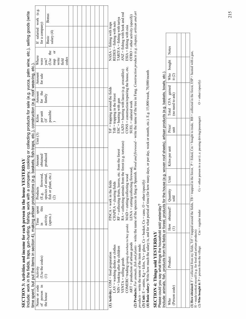
21
5
SEC
TIO
N 3
: Act
iviti
es a
nd in
com
e fo
r ea
ch p
erso
n in
the
hous
e Y
EST
ER
DA
Y
Incl
ude:
wor
k in
the
field
s, tr
aps,
gun
-hun
ting,
fish
ing,
wor
k w
ith a
com
pany
, coo
king
or
colle
ctin
g pr
oduc
ts fo
r sa
le (
e.g.
yuc
ca, p
alm
win
e, e
tc.),
sel
ling
good
s (w
rite
time
spen
t, bu
t put
the
item
s in
sec
tion
4), m
akin
g ar
tisan
pro
duct
ions
(e.g
. bas
kets
, fis
h-tra
ps, e
tc.),
con
stru
ctio
n (e
.g. r
oof w
eavi
ng, e
tc.).
If
sala
ried
wor
k (e
.g.
for a
com
pany
) N
ame
or c
ode
of
pers
on
in
the
hous
e
Act
ivity
(U
se th
e co
des)
(1
)
Tim
e sp
ent
in
this
activ
ity
(apr
ox.)
Prod
ucts
(E
.g.
firew
ood,
sp
ecie
s of
ani
mal
, fis
h or
pla
nt, e
tc.)
(2)
Am
ount
ob
tain
ed/
prod
uced
Uni
t (3)
K
ilos
per u
nit
(if
poss
ible
)
Am
ount
fo
r th
e fa
mily
Am
ount
fo
r sal
e
Whe
re
wer
e yo
u?
(Use
th
e m
ap
or
writ
e fie
ld
code
s
Bas
ic
sala
ry (4
) B
onus
(1) A
ctiv
ity: C
OM
= fo
od p
repa
ratio
n
FI
NC
A =
wor
k in
the
field
s
TrF
= tra
ppin
g ar
ound
the
field
s
NA
SA =
fish
ing
with
trap
s LA
V =
was
hing
dis
hes o
r clo
thes
CH
APE
A =
cle
arin
g fie
lds
Tr
B =
trap
ping
in th
e fo
rest
RED
ES =
fish
ing
with
net
s N
IN =
look
ing
afte
r the
chi
ldre
n
RF
= co
llect
ing
frui
ts, le
aves
, etc
. fro
m th
e fo
rest
ES
C =
hun
ting
with
gun
TAR
IYA
= fi
shin
g w
ith ta
riya
VEN
TA =
sel
ling
good
s
R
A =
col
lect
ing
anim
als f
rom
the
fore
st (e
.g. t
orto
ises
) LA
ZO =
hun
ting
with
lass
o (e
.g. c
roco
dile
s)
AN
Z =
fishi
ng w
ith h
ook
and
rod
CO
MER
C=t
radi
ng (g
oing
els
ewhe
re to
buy
goo
ds)
MA
D =
cut
ting/
colle
ctin
g w
ood
CO
NS
= co
nstru
ctio
n/re
pairi
ng th
e ho
use,
etc
. ES
IA =
fish
ing
with
esi
a A
RT
= pr
oduc
tion
of a
rtisa
n go
ods
LE
NA
= c
uttin
g/co
llect
ing
firew
ood,
SU
EL =
sal
arie
d w
ork
OTR
O =
oth
er a
ctiv
ity (s
peci
fy)
(2) P
rodu
cts:
For
ani
mal
s, fi
sh a
nd p
lant
s � w
rite
the
nam
e of
the
spec
ies i
n fa
ng o
r Spa
nish
. Woo
d an
d fir
ewoo
d �
writ
e th
e na
me
of th
e tre
e in
Fan
g. C
onst
ruct
ion
prod
ucts
(e.g
. cha
pas)
, arti
san
and
art
prod
ucts
� w
rite
the
nam
e of
the
item
mad
e.
(3) U
nit:
E =
ent
ire, K
g =
kilo
s, V
a =
glas
s, C
e =
bask
et, C
n =
cane
, O =
oth
er (s
peci
fy)
(4
) Bas
ic sa
lary
: Writ
e ho
w m
uch
the
sala
ry is
, and
for w
hat p
erio
d of
tim
e (f
or h
ow m
any
days
, or p
er d
ay, w
eek
or m
onth
, etc
.). E
.g. 1
5,00
0/w
eek,
70,
000/
mon
th
SEC
TIO
N 4
: Thi
ngs s
old
YE
STE
RD
AY
Pl
ease
cou
ld y
ou s
ay w
hat t
hing
s th
e ho
useh
old
sold
yes
terd
ay?
Incl
ude:
ani
mal
s, fi
sh, p
rodu
cts
from
the
field
s or
fore
st, p
rodu
cts
for t
he h
ouse
(e.g
. wov
en ro
of s
heet
s), a
rtisa
n pr
oduc
ts (e
.g. b
aske
ts, b
owls
, etc
.).
Who
(P
erso
n co
de)
Prod
uct
H
ow
obta
ined
? (1
) Q
uant
ity
sold
U
nit
Kilo
s per
uni
t Pr
ice/
un
it To
tal
CFA
ga
ined
(n
o ne
ed to
ask
) W
ho
boug
ht
it (2
) N
otes
(1) H
ow o
btai
ned:
F =
col
lect
ed fr
om m
y fie
lds,
TrF
= tra
pped
aro
und
the
field
s, TB
= tr
appe
d in
the
fore
st, P
= fi
shed
, Cm
= b
ough
t to
trade
, R
B =
col
lect
ed in
the
fore
st, E
SP =
hun
ted
with
a g
un,
H =
mad
e/co
oked
mys
elf (
e.g.
for f
ood
and
artis
an p
rodu
cts)
(2
) Who
bou
ght i
t: P
= p
erso
n fr
om th
e vi
llage
C
m =
regu
lar t
rade
r
Cc
= ot
her p
erso
n in
a c
ar (i
..e. p
assi
ng d
rivin
g/pa
ssen
ger)
O
= o
ther
(spe
cify
)

21
6
Tab
le A
1.3
Que
stio
nnai
res o
n bu
ildin
gs, f
ixed
ass
ets,
and
fam
ily re
mitt
ance
s ove
r the
yea
r.
Vill
age:
In
terv
iew
er(s
): St
art t
ime:
End
tim
e:
Hou
seho
ld c
ode:
In
terv
iew
ee(s
): D
ate:
1.
Bui
ldin
gs
Is th
e ho
use
whe
re y
ou li
ve y
ours
?
Do
you
rent
any
oth
er b
uild
ings
(e.g
. bar
s, e
tc.)
If no
, who
doe
s it
belo
ng to
?
G
ive
deta
ils o
f tho
se b
uild
ings
D
o yo
u pa
y re
nt?
H
ow m
uch
rent
do
you
pay
for t
hese
? H
ow m
uch?
W
ho d
oes
it be
long
to?
For b
ldgs
in th
is v
illag
e�
Type
of
bu
ildin
g (1
)
Whi
ch
kitc
hen
Whe
re
(whi
ch
villa
ge)
How
old
is
it (y
rs)
Who
bo
ught
th
e m
ater
ials
(2
) O
wne
r (3)
R
espo
nsib
le
(4)
How
m
any
bedr
oom
s?
Floo
r (5
) R
oof
(6)
Wal
ls
(7)
How
m
any
door
s (8
) H
ow
man
y w
indo
ws
(9)
Con
ditio
n (1
0)
(1)
Type
of
build
ing:
V=
hous
e, C
o= k
itche
n, C
P= t
alki
ng h
ut,
Br=
bar,
Bn =
toi
let/
bath
room
(2
) Who
bou
ght t
he m
ater
ials
? Fo
= re
lativ
e w
ho li
ves
in e
lsew
here
, Fp
= re
lativ
e w
ho
lives
in th
is v
illage
(in
a di
ffere
nt h
ouse
), EC
= th
is h
ouse
(writ
e th
eir p
erso
nal c
ode)
(3
) Ow
ner:
The
per
son
who
ow
ns th
e bu
ildin
g (4
) Res
pons
ible
: The
per
son
who
is re
spon
sibl
e fo
r the
bui
ldin
g. T
hat i
s, if
you
wer
e to
re
nt th
e bu
ildin
g, w
ho w
ould
gai
n th
e m
oney
?
(5) F
loor
: Ti =
mud
, Ce
= ce
men
t, C
a =
woo
den
pane
ls, T
a =
woo
d pl
anks
, B =
tile
s (6
) Roo
f: N
= th
atch
, Ch
= co
rruga
ted
iron,
S =
Woo
d pa
nels
and
cor
ruga
ted
iron
(7) F
loor
: Ta
= W
ord
plan
ks, C
e =
cem
ent,
N =
that
ch, C
a =
woo
d pa
nels
, NE
= m
unse
-es
í (ba
rro),
L =
tiles
, P =
pre
-fabr
icat
ed s
heet
s (8
) How
man
y do
ors?
: S=
sim
ple,
EPS
= en
tre-p
año
sim
ple,
EPM
= e
ntre
-pañ
o m
odel
o (9
) How
man
y w
indo
ws?
: S =
sim
ple,
EP
= en
tre-p
año,
P =
per
sian
a (1
0) C
ondi
tion:
T =
unf
inis
hed,
B =
goo
d, N
P =
unin
habi
tabl
e D
oes
anyo
ne re
nt a
room
/hou
se/b
ar/o
ther
bui
ldin
g fro
m y
ou/y
our f
amily
? H
ow d
o th
ey p
ay?
Alw
ays:
NLS
= D
on�t
know
NQ
C =
Don
�t w
ant t
o re
ply

217
2. Goods/possessions
Item Type and
amount Which kitchen How old is it? Condition
(1)
How was it obtained (2)
Price when bought (write ~ and guess if unknown)
Total price (no need to ask)
Cooking apparatus L = wood fire HG = gas fire H = over
Bed and mattresses Ma-D = soft wood Ma-F = hard wood B = bamboo CE = Sponge mattress CM = mattress with springs CP = feather mattress
Chairs and seats Ma = wood Me = rattan/wicker P = plastic B = bamboo S = sofa/trisillio/salón
Water source R = river, M = spring P = well
Fridges and freezers Radio, radio-CD, radio-cassette
Saucepans (g=big, m=medium, p= small)
Grinders and wheelbarrows
Television, video Chainsaw, gun, rifle Bicycle, car, motorbike Generator
(1) (2) Condition: 1 = good, 2 = a bit bad, but still usable, 3 = broken (unusable) (3) How was it obtained?: Co = bought by someone in this house, Co-Fp = bought by family member in this village (and is still theirs), Co-Fo
= bought by family member from elsewhere, RgFo = gift from family from elsewhere, RgFp = gift frm faily from this village, Hd = inherited, Hc = made
Domestic animals (Include adults only) Kitchen Chicken Goat Sheep Duck Cat Dog Pig Other

218
Household code: Interviewer(s): Date:
Village: Interviewee(s): Start time: End time:
3. Money/help that left the house in 2005
People that are supported by this household�
Person (number)
Relation (1)
Kitchen Where do they live?
Working status (2)
Type of help Value (CFA) Frequency in 2005
Total CFA (no need to ask)
4. Money/help that entered the house in 2005
People that contribute to the household� Person (number)
Relation (1)
Kitchen Where do they live?
Profession/work (3)
Type of help Value (CFA) Frequency in 2005
Total CFA (no need to ask)
(1) Relation: J = jefe/a residencial Hj = hijo/a Y = yerno/nuera T = tío/a M = marido/mujer/compañero Hm = hermano/a Cu = cuñado/a So = sobrino/a
N = nieto/a Pd = padre/madre Sg = suegro/a Pm =primo/a A = abuelo/a C = otro compañero Ot = otro no familia (declare que)
(2) Work status: Es = student, T = working, BT = looking for work, VM = lives with husband, VA = lives with boyfriend (3) Profesión/work: Ma = manual work, T = technical work, Of = office work, M/P = teacher, Mi = military, G = work in the government, D = director, BT = looking for work, VM = lives with husband that works (write what type of work he has), VA = lives with boyfriend that works (write type)

Appe
ndice
s
Alleb
one-
Web
b, S
.M. (
2009
) Eva
luatin
g de
pend
ence
on
wildl
ife p
rodu
cts in
rura
l Equ
ator
ial G
uinea
219
Appendix
2.
Agri
cultura
l cale
ndar
Tab
le A
2.1
Agr
icul
tura
l cal
enda
r M
onth
Ja
n Fe
b M
ar
Apr
M
ay
Jun
Ju
Aug
S
ep
Oct
N
ov
Dec
R
ain
Lots
Littl
e
Littl
e
Littl
e
Littl
e
Ata
nga
Har
vest
Fr
uitin
g
B
anan
a H
arve
st
C
alab
aza
~2 d
ays
3x
3 da
ys
Cho
cola
te
Fr
uitin
g
Har
vest
Fo
rest
frui
ts
Har
vest
(E
aten
dec
- fe
b)
M
aiz
2 da
ys
3
wee
ks
3 w
eeks
Mal
anga
M
ango
1 S
ome
man
goes
har
vest
ed a
ll ye
ar ro
und,
but
mos
t in
Nov
embe
r
O
rang
e
P
eanu
t
Pin
eapp
le
Pla
ntai
n H
arve
st
S
ugar
can
e H
arve
st
V
erdu
ras
gree
ns
Yam
H
arve
st
Y
uca
H
arve
st
Fi
sh (t
ariy
a)2
Fish
(tr
ap
and
rod)
H
unt (
trap)
3
H
unt (
gun)
4
G
ener
al fo
od5
Cle
ar fi
elds
: men
W
eedi
ng: w
omen
B
urni
ng
KE
Y
C
ultiv
atio
n/Pl
antin
g
C
lear
ing/
wee
ding
fiel
ds
M
ost f
ood
Har
vest
Fi
elds
bur
nt fo
r cle
arin
g
Less
food
M
ore
anim
als/
fish
caug
ht
M
uch
rain
Leas
t foo
d
Less
ani
mal
s/fis
h ca
ught
Som
e ra
in
2 da
ys
4 day
s
Har
vest
ed a
ll ye
ar, 2
mon
ths a
fter p
lant
ing

Appendices
Allebone-Webb, S.M. (2009) Evaluating dependence on wildlife products in rural Equatorial Guinea 220
Appendix 3. Calculating building costs
Table A 3.1 An example of the cost of building a five bedroom house in Teguete (i.e. 6 rooms, no kitchen, no bathroom). All prices are shown in CFA (1000cfa = £1.03, December 2006).
Item Description Cost Per Item
No. Needed
Total Cost/ House
Wooden planks Made of soft wood harvested in the forest, and used overlapping for the walls
250 400 100000
Transport for wooden planks
Transport from the forest to the village (some people choose to carry it back themselves).
50 400 20000
Corrugated iron sheets
For roof 2700 109 294300
Vertical beams House structure 300 80 24000
Roof support House structure 350 100 35000
Horizontal beams House structure 350 78 27300
Window shutters All wooden
- Slatted 15000 0
- Decorated 10000 0
- Simple 4000 12 48000
Doors
- EP simple Harder wood, simple design 17500
- EP modelo Harder wood, patterned 25000
- Simple Soft wood, simple design 2500 7 17500
Nails Bought per Kg 1000/kg 30 30000
Hinges 500 14 7000
Locks and latches 500 7 3500
Carpenter To cut and prepare the wood 100000 1 100000
To construct the skeleton and roof 200000 1 200000
To put the rest of the walls on (most people do it themselves)
TOTAL 906600
OTHER materials sometimes used
Ceiling (�sierra�) Ceiling made from thinner wooden strips (literally �cut with chainsaw�).
Nipas Palm roofing made by weaving palm fronds. People often make their own, but some people sell them.
300

Appendices
Allebone-Webb, S.M. (2009) Evaluating dependence on wildlife products in rural Equatorial Guinea 221
Nde-bevin Tree bark used as wall Us. collected, not sold
Nde-esi Mud bricks used as wall Us. collected, not sold
Calabo Thin strips of wood used for wall or flooring
Cement For floors
Breeze blocks For walls
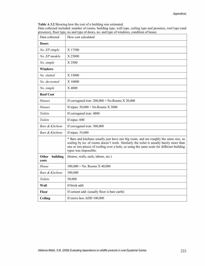
Appendices
Allebone-Webb, S.M. (2009) Evaluating dependence on wildlife products in rural Equatorial Guinea 222
Table A 3.2 Showing how the cost of a building was estimated. Data collected included: number of rooms, building type, wall type, ceiling type and presence, roof type (and presence), floor type, no and type of doors, no. and type of windows, condition of house.
Data collected How cost calculated
Doors
No. EP simple X 17500
No. EP modelo X 25000
No. simple X 2500
Windows
No. slatted X 15000
No. decorated X 10000
No. simple X 4000
Roof Cost
Houses If corrugated iron: 200,000 + No.Rooms X 20,000
Houses If nipas: 30,000 + No.Rooms X 3000
Toilets If corrugated iron: 4800
Toilets If nipas: 600
Bars & Kitchens If corrugated iron: 300,000
Bars & Kitchens If nipas: 35,000
* Bars and kitchens usually just have one big room, and are roughly the same size, so scaling by no. of rooms doesn�t work. Similarly the toilet is usually barely more than one or two pieces of roofing over a hole, so using the same scale for different building types was impossible.
Other building costs
(beams, walls, nails, labour, etc.)
House 300,000 + No. Rooms X 40,000
Bars & Kitchens 300,000
Toilets 50,000
Wall If brick add:
Floor If cement add: (usually floor is bare earth)
Ceiling If sierra laso ADD 100,000

Appendices
Allebone-Webb, S.M. (2009) Evaluating dependence on wildlife products in rural Equatorial Guinea 223
Appendix 4. List of material assets recorded
Table A 4.1 A list and number of items recorded as material assets in each village.
Beayop Teguete
Item Total number in
village
Average price per item (cfa)
Total number in
village
Average price per item (cfa)
Kitchen items Grinder (for peanuts & calabaza) 80 13794.05 66 16370.02 GasCooker 4 18750 5 7000 Cooking pot - large 197 5000 196 5000 Cooking pot - medium 1609 3500 1315 3500 Cooking pot - small 156 2000 109 2000 Press (for clothes) 1 4000 0
Livelihood equipment Press (for sugar cane) 24 3350 0 Bread oven 1 40000 0 Bar - wooden (in shop) 7 2500 1 150000 Wheelbarrow 27 28350 23 22777.78 Escopeta 5 156666.7 8 148000 Motosierra 5 255000 5 520000 SewingMachine 1 5000 4 6250 Bicycle 2 40000 14 69142.86 Bicycle - wooden 1 10000 0 Freezer 2 245000 6 250000
Furniture Bed - wood 105 16530.61 14 5000 Bed - bamboo 568 2390.164 14 2390.164 Bed - metal 11 22000 0 Bed - soft wood 145 10351.06 600 3850 Bed - hard wood 97 19928.57 66 23541.67 Chair - bamboo 3 3333.333 0 Chair - metal 28 2264.706 4 2264.706 Chair - plastic 56 5407.407 144 5200 Chair - wicker 78 3444.444 46 5886.364 Chair - wood 152 4071.429 364 3370.879 Chair - soft wodd 18 31428.57 13 31428.57 Chair - hard wood 6 2000 9 5000 Mattress - feather 1 30000 0 Mattress - sponge 424 20522.81 387 25608.11 Mattress - springs 8 30000 0 Chair set - wicker 57 25185.19 3 15000 Sofa 6 8333.333 8 10000 Table - wood 2 15000 1 30000 Sofa set (1 sofa, 2 armchairs) 27 165224.2 15 74000 Wardrobe 2 110000 1 5000 Continued on next page
Item (continued) Beayop Teguete

Appendices
Allebone-Webb, S.M. (2009) Evaluating dependence on wildlife products in rural Equatorial Guinea 224
Total number in
village
Average price per item (cfa)
Total number in
village
Average price per item (cfa)
Domestic animals Goat 50 20000 129 20000 Pig 44 40000 0 Hen 540 2000 431 2000 Cat 84 0 24 0 Sheep 21 18000 25 18000 Duck 52 2500 62 2500 Dog 10 0 21 0
Entertainment DVD 1 150000 0 Music system 2 145000 0 Radio 10 11900 30 14315.48 Radio Cassette 64 25420 45 24236.81 Radio CD 1 80000 2 60000 TV 10 139285.7 4 100000 TV Video 1 120000 0 Video 3 20000 4 20000
Fields Peanuts and mixed crop 289 72 Calabaza and mixed crop 188 214 Peanut & Calabaza 3 2 Pineapple 4 20 Mixed tree crops (avocados, palm, etc) 1 3
Other Lawn trimmer 2 625000 0 Generator 20 140735.3 17 283294.1 Gas lamp 270 3500 105 3500 Torches 89 1000 23 1000

Appendices
Allebone-Webb, S.M. (2009) Evaluating dependence on wildlife products in rural Equatorial Guinea 225
Appendix 5. Supplementary tables: Chapter 3
Total calories/day/individual (offset by individual AME) Table A 5.1 Results of linear mixed model (LMM) showing correlation of daily calorie consumption per individual with season, and individual and household level variables. Individual nested within household, within village specified as random effects. AME specified as offset. Parameter estimates shown for significant variables in the minimum adequate model (MAM). Explanatory variables were transformed to give normal distributions, and these transformations are shown in brackets. Explanatory variables were transformed in the same way for all other analyses. Results shown in brackets were not included in the MAM due to insignificance (where p >0.05) or correlation with another explanatory variable (where more than one correlated explanatory variable significantly varied with the data, only the one explaining the greater part of the data was included in the MAM).
Variable Level Parameter estimate d.f. Deviance
change P
intercept 6.01
Season 1 Little Dry 2 First Wet 3 Big Dry 4 Second Wet
0 -0.074 -0.13 0.032
3 15 p < 0.005
Village Beayop Teguete
0 -0.10
1 5 p < 0.05
HH Income (log) 0.034 1 4 p < 0.05
Fixed Wealth (sqrt) 0.000055 1 38 p < 0.0001
Wealth rank (factor) 3 1 ns
HH size (sqrt) -0.17 1 31 p < 0.0001
No. productive adults (sqrt) 1 (5) (p < 0.05)
No. productive females (sqrt) 1 (10) (p < 0.01)
Productive males (yes/no) 1 2 ns
Proportion productive adults (sqrt(asin()) 1 (5) (p < 0.05)
Proportion productive female (sqrt(asin()) 0.17 1 6 p < 0.02
Sex 1 3 ns
Age (sqrt) 0.018 1 36 p < 0.0001
HH head sex 1 4 (p = 0.052)
HH head education 3 2 ns
Variance: Individual = 0, HH = 0.03, Village = 0.0002, Season = 0.0003, Residual variance = 0.15 n (Village) = 2, n (HH) = 144 n (individual) = 966, n (season) = 4, n (observations) = 4797

Appendices
Allebone-Webb, S.M. (2009) Evaluating dependence on wildlife products in rural Equatorial Guinea 226
Total protein/day/individual (offset by individual AME) Table A 5.2 Results of linear mixed model showing correlation of daily protein consumption (g) per individual with season, and individual and household level variables. Individual nested within household, within village specified as random effects. AME specified as offset. Parameter estimates shown for significant variables in the MAM.
Variable Level Parameter estimate d.f. Deviance
change P
intercept 2.39
Season 1 Little Dry 2 First Wet 3 Big Dry 4 Second Wet
0 -0.073 -0.070 0.031
3 8 p < 0.05
Village Beayop Teguete
0 -0.17
1 5 p < 0.05
HH Income 0.058 1 5 p < 0.05
Fixed Wealth 0.00015 1 106 p < 0.0001
Wealth rank 3 2 ns
HH size -0.016 1 11 p < 0.005
No. productive adults 1 0 ns
No. productive females 1 1 ns
Productive males (yes/no) 1 3 (p = 0.09)
Proportion productive adults 1 1 ns
Proportion productive females 0.23 1 4 p < 0.05
Sex 1 1 ns
Age 0.014 1 9 p < 0.005
HH head sex 1 1 ns
HH head education 3 2 ns
Variance: Individual = 0, HH = 0.09, Village = 0.0005, Season = 0.0009, Residual variance = 0.39 n (Village) = 2, n (HH) = 144 n (individual) = 966, n (season) = 4, n (observations) = 4797

Appendices
Allebone-Webb, S.M. (2009) Evaluating dependence on wildlife products in rural Equatorial Guinea 227
Total calories/day/household Table A 5.3 Results of linear mixed model showing the correlation of daily household calorie consumption/AME with season and household level variables. Household nested within village specified as a random effect. Parameter estimates shown for significant variables in the minimum adequate model.
Variable Levels Parameter values d.f. Deviance
change P
Intercept 7.63
Season 1 Little Dry 2 First Wet 3 Big Dry 4 Second Wet
-0.13 -0.16 0.087
3 8 p < 0.05
Village 1 3 (p = 0.087)
Wealth rank 3 2 ns
Fixed wealth 0.00014 1 48 p < 0.0001
HH Income 1 1 ns
HH size -0.17 1 22 p < 0.0001
No. productive adults 1 1 ns
No. productive females 1 0 ns
Productive males (yes/no) 1 1 ns
Proportion productive adults 1 3 ns
Proportion productive females 1 3 (p = 0.053)
Household head sex 1 3 ns
Household head education 3 0 ns
Variance: HH = 0.034, Season = 0.0019, Village = 0.0045, Residual variance = 0.19 n (Village) = 2, n (Season) = 4, n (Household) = 146, n (Observations) = 1085
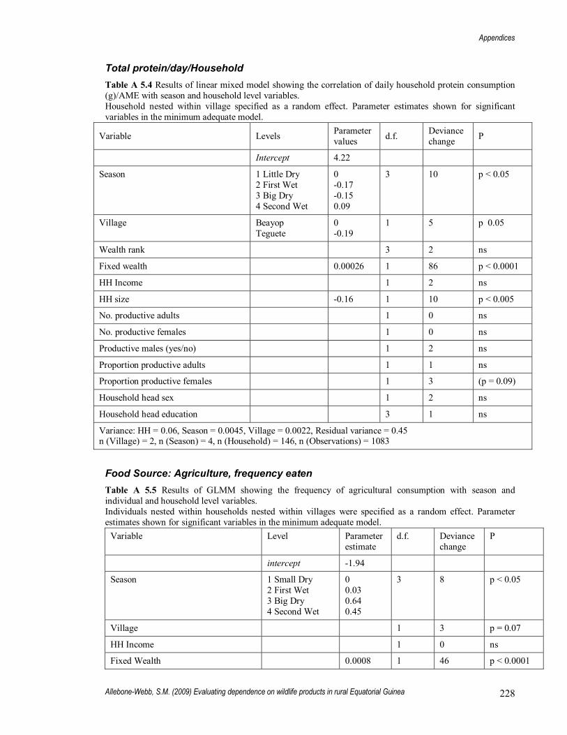
Appendices
Allebone-Webb, S.M. (2009) Evaluating dependence on wildlife products in rural Equatorial Guinea 228
Total protein/day/Household Table A 5.4 Results of linear mixed model showing the correlation of daily household protein consumption (g)/AME with season and household level variables. Household nested within village specified as a random effect. Parameter estimates shown for significant variables in the minimum adequate model.
Variable Levels Parameter values d.f. Deviance
change P
Intercept 4.22
Season 1 Little Dry 2 First Wet 3 Big Dry 4 Second Wet
0 -0.17 -0.15 0.09
3 10 p < 0.05
Village Beayop Teguete
0 -0.19
1 5 p 0.05
Wealth rank 3 2 ns
Fixed wealth 0.00026 1 86 p < 0.0001
HH Income 1 2 ns
HH size -0.16 1 10 p < 0.005
No. productive adults 1 0 ns
No. productive females 1 0 ns
Productive males (yes/no) 1 2 ns
Proportion productive adults 1 1 ns
Proportion productive females 1 3 (p = 0.09)
Household head sex 1 2 ns
Household head education 3 1 ns
Variance: HH = 0.06, Season = 0.0045, Village = 0.0022, Residual variance = 0.45 n (Village) = 2, n (Season) = 4, n (Household) = 146, n (Observations) = 1083
Food Source: Agriculture, frequency eaten Table A 5.5 Results of GLMM showing the frequency of agricultural consumption with season and individual and household level variables. Individuals nested within households nested within villages were specified as a random effect. Parameter estimates shown for significant variables in the minimum adequate model.
Variable Level Parameter estimate
d.f. Deviance change
P
intercept -1.94
Season 1 Small Dry 2 First Wet 3 Big Dry 4 Second Wet
0 0.03 0.64 0.45
3 8 p < 0.05
Village 1 3 p = 0.07
HH Income 1 0 ns
Fixed Wealth 0.0008 1 46 p < 0.0001

Appendices
Allebone-Webb, S.M. (2009) Evaluating dependence on wildlife products in rural Equatorial Guinea 229
Wealth rank 1 2 3 4 5
0 -0.35 -0.38 -1.92 -2.87
1 32 p < 0.0001
HH size 2.38 1 27 p < 0.0001
No. productive adults 1 (19) (p < 0.01)
No. productive females 1 (10) (p < 0.01)
Productive males (yes/no) 1 0 ns
Proportion productive adults 1 1 ns
Proportion productive females 1.65 1 5 p < 0.05
Sex 1 1 ns
Age (sqrt) 1 2 ns
Education 3 0 ns
HH head sex 1 1 ns
HH head education 3 8 (p = 0.053)
Variance: Individual = 0, Household = 5.52, Season = 0.0001, Village = 0 N: Season = 4, Village = 2, Household = 145, Individuals = 878, Observations = 5026
Food Source: Agriculture, proportion calories Table A 5.6 Results of LMM showing the correlation of proportion of calories consumed from agriculture with season and individual and household level variables. The arc-sin of the proportion of calories was taken to give a normal distribution. Individuals nested within households nested within villages were specified as a random effect. Parameter estimates shown for significant variables in the minimum adequate model.
Variable Level Parameter estimate d.f. Deviance
change P
intercept 0.59
Season 1 Small Dry 2 First Wet 3 Big Dry 4 Second Wet
-0.025 0.028 -0.021
3 20 p < 0.001
Village 1 4 (p = 0.054)
HH Income 1 0 ns
Fixed Wealth 0.000018 1 41 p < 0.0001
Wealth rank 1 2 3 4 5
0.097 0.088 -0.028 -0.19
1 18 p < 0.005
HH size 1 2 ns
No. productive adults 1 1 ns
No. productive females 1 1 ns

Appendices
Allebone-Webb, S.M. (2009) Evaluating dependence on wildlife products in rural Equatorial Guinea 230
Productive males (yes/no) 1 0 ns
Proportion productive adults 1 1 ns
Proportion productive females 1 2 ns
Sex 1 1 ns
Age 1 0 ns
Education 3 2 ns
HH head sex 1 2 ns
HH head education 3 3 ns
Variance: Individual = 0, Household = 0.026, Village = 0.0018, residual variance = 0.12 N: Season = 4, Village = 2, Household = 145, Individuals = 873, Observations = 4815
Food Source: Agriculture, proportion protein Table A 5.7 Results of LMM showing the correlation of proportion of protein consumed from agriculture with season and individual and household level variables. The arc-sin of the proportion of protein was taken to give a normal distribution. Individuals nested within households nested within villages were specified as a random effect. Parameter estimates shown for significant variables in the minimum adequate model.
Variable Level Parameter estimate d.f. Deviance
change P
intercept 0.76
Season 1 Small Dry 2 First Wet 3 Big Dry 4 Second Wet
3 8 (p = 0.050)
Village Beayop Teguete
0.085
1 5 p < 0.05
HH Income -0.032 1 47 p < 0.0001
Fixed Wealth 1 3 ns
Wealth rank 1 2 3 4 5
1 8 (p = 0.069)
HH size 1 0 ns
No. productive adults 1 0 ns
No. productive females 1 0 ns
Productive males (yes/no) 1 2 ns
Proportion productive adults 1 1 ns
Proportion productive females 1 4 (p = 0.063)
Sex 1 ns
Age 1 ns
Education 3 ns

Appendices
Allebone-Webb, S.M. (2009) Evaluating dependence on wildlife products in rural Equatorial Guinea 231
HH head sex 1 ns
HH head education 3 2 ns
Variance: Individual = 0, Household = 0.026, Village = 0.00013, residual variance = 0.12 N: Season = 4, Village = 2, Household = 149, Individuals = 892, Observations = 4869
Food Source: Bought, frequency eaten Table A 5.8 Results of GLMM showing the frequency of bought food consumption with season and individual and household level variables. Individuals nested within households nested within villages were specified as a random effect. Parameter estimates shown for significant variables in the minimum adequate model.
Variable Level Parameter estimate d.f. Deviance
change P
intercept -5.59
Season 1 Small Dry 2 First Wet 3 Big Dry 4 Second Wet
3 3 ns
Village Beayop Teguete
0 -1.02
1 8 p < 0.01
HH Income 0.55 1 10 p < 0.005
Fixed Wealth 1 4 ns
Wealth rank (+) 1 8 (p = 0.09)
HH size 1 3 ns
No. productive adults 1.05 1 9 p < 0.005
No. productive females 1 4 (p = 0.09)
Productive males (yes/no) 1 7 (p < 0.005)
Proportion productive adults 1 1 ns
Proportion productive females 1 -1 ns
Sex 1 0 ns
Age -0.06 1 9 p < 0.005
Education 3 2 ns
HH head sex 1 1 ns
HH head education 3 5 ns
Variance: Individual = 0, Household = 2.12, Village = 0.00013 N: Season = 4, Village = 2, Household = 144, Individuals = 931, Observations = 5120

Appendices
Allebone-Webb, S.M. (2009) Evaluating dependence on wildlife products in rural Equatorial Guinea 232
Food Source: Gifts, frequency eaten Table A 5.9 Results of GLMM showing the frequency of gift food consumption with season and individual and household level variables. Individuals nested within households nested within villages were specified as a random effect. Parameter estimates shown for significant variables in the minimum adequate model.
Variable Level Parameter estimate d.f. Deviance
change P
intercept -4.34
Season 1 Small Dry 2 First Wet 3 Big Dry 4 Second Wet
-0.77 -0.58 -0.86
3 38 p < 0.0001
Village Beayop Teguete
1 1 ns
HH Income 1 1 ns
Fixed Wealth 1 -316 ns
Wealth rank 1 2 3 4 5
0 -0.86 -0.99 -0.60 0.052
1 36 p < 0.0001
HH size -0.42 1 17 p < 0.0001
No. productive adults 1 2 ns
No. productive females 1 2 ns
Productive males (yes/no) 1 1 ns
Proportion productive adults 1 3 ns
Proportion productive females 1 1 ns
Sex 1 0 ns
Age 1 3 (p = 0.07)
Education 3 1 ns
HH head sex 1 5 (p = 0.08)
HH head education 3 5 ns
Variance: Individual = 0, Household = 1.47, Village = 0 N: Season = 4, Village = 2, Household = 151, Individuals = 955, Observations = 5196
Food Source: Forest (all), frequency eaten Table A 5.10 Results of GLMM showing the frequency of forest food source consumption with season and individual and household level variables. Individuals nested within households nested within villages were specified as a random effect. Parameter estimates shown for significant variables in the minimum adequate model.
Variable Level Parameter estimate d.f. Deviance
change P
intercept -3.13

Appendices
Allebone-Webb, S.M. (2009) Evaluating dependence on wildlife products in rural Equatorial Guinea 233
Season 1 Small Dry 2 First Wet 3 Big Dry 4 Second Wet
0 -1.93 -1.86 0.22
3 15 p < 0.005
Village Beayop Teguete
1.14
1 11 p < 0.001
Season: Village T: 1 Small Dry T: 2 First Wet T: 3 Big Dry T: 4 Second Wet
2.07 2.31 -0.29
3 172 p < 0.0001
HH Income -0.014 1 129 p < 0.0001
Fixed Wealth 1 -327 ns
Wealth rank 1 7 (p = 0.069)
HH size 1.19 1 36 p < 0.0001
No. productive adults 1 11 (p < 0.001)
No. productive females 1 14 (p < 0.001)
Productive males (yes/no) 1 1 ns
Proportion productive adults 1 6 (p < 0.05)
Proportion productive females 1 0 ns
Sex 1 0 ns
Age 1 0 ns
Education 3 3 ns
HH head sex 1 0 ns
HH head education 3 5 (p = 0.052)
Variance: Individual = 0, Household = 1.57, Village = 0 N: Season = 4, Village = 2, Household = 150, Individuals = 879, Observations = 5057
Food Source: Forest (all), proportion protein Table A 5.11 Results of LMM showing the correlation of proportion of protein consumed from forest food sources with season and individual and household level variables. The arc-sin of the proportion of protein was taken to give a normal distribution. Individuals nested within households nested within villages were specified as a random effect. Parameter estimates shown for significant variables in the minimum adequate model.
Variable Level Parameter estimate d.f. Deviance
change P
intercept 0.22
Season 1 Small Dry 2 First Wet 3 Big Dry 4 Second Wet
0 0.15 0.20 -0.06
3 39 p < 0.0001
Village Beayop Teguete
0.05
1 1 ns

Appendices
Allebone-Webb, S.M. (2009) Evaluating dependence on wildlife products in rural Equatorial Guinea 234
Season: Village T: 1 Small Dry T: 2 First Wet T: 3 Big Dry T: 4 Second Wet
-0.12 -0.17 0.12
3 15 p < 0.005
HH Income 1 -2 ns
Fixed Wealth 1 3 (p = 0.067)
Wealth rank 1 3 ns
HH size 1 0 ns
No. productive adults 1 1 ns
No. productive females 1 0 ns
Productive males (yes/no) 1 (6) (p < 0.01)
Proportion productive adults 1 0 ns
Proportion productive females 1 0 ns
Sex 1 1 ns
Age 1 1 ns
Education 3 1 ns
HH head sex Female Male
0.12
1 8 p < 0.005
HH head education 3 2 ns
Variance: Individual = 0, Household = 0.038, Village = 0.00023, residual variance = 0.10 N: Season = 4, Village = 2, Household = 123, Individuals = 718, Observations = 2348
Food Source: Forest (all), proportion calories Table A 5.12 Results of LMM showing the correlation of proportion of calories consumed from forest food sources with season and individual and household level variables. The arc-sin of the proportion of calories was taken to give a normal distribution. Individuals nested within households nested within villages were specified as a random effect. Parameter estimates shown for significant variables in the minimum adequate model. The difference in sample size between models of proportion of protein and proportion of calories are due to the foods eaten containing no protein (i.e. some forest fruits contain no protein)
Variable Level Parameter estimate d.f. Deviance
change P
intercept 0.12
Season 1 Small Dry 2 First Wet 3 Big Dry 4 Second Wet
0 0.08 0.03 -0.06
3 131 p < 0.0001
Village Beayop Teguete
0 0.06
1 5 p < 0.05
HH Income 1 -68 ns
Fixed Wealth 1 -37 ns
Wealth rank 1 4 ns
HH size 1 3 (p = 0.097)

Appendices
Allebone-Webb, S.M. (2009) Evaluating dependence on wildlife products in rural Equatorial Guinea 235
No. productive adults 1 1 ns
No. productive females 1 3 ns
Productive males (yes/no) 1 0 ns
Proportion productive adults 1 1 ns
Proportion productive females 1 0 ns
Sex 1 0 ns
Age 1 1 ns
HH head sex Female Male
1 3 (p = 0.062)
HH head education 3 2 ns
Variance: Individual = 0, Household = 0.006, Village = 0.00005, residual variance = 0.022 N: Season = 4, Village = 2, Household = 125, Individuals = 732, Observations = 2387
Food Source: Forest animal, frequency eaten Table A 5.13 Results of GLMM showing the frequency of forest animal consumption with season and individual and household level variables. Individuals nested within households nested within villages were specified as a random effect. Parameter estimates shown for significant variables in the minimum adequate model.
Variable Level Parameter estimate d.f. Deviance
change P
intercept -16.29
Season 1 Small Dry 2 First Wet 3 Big Dry 4 Second Wet
0 -0.95 -0.13 -0.34
3 13 p < 0.005
Village Beayop Teguete
0 2.08
1 10 p < 0.005
HH Income 0.59 1 40 p < 0.0001
Fixed Wealth 1 -349 ns
Wealth rank 1 2 3 4
0 1.59 0.38 -0.59
1 13 p < 0.01
HH size 1.20 1 11 p < 0.005
No. productive adults 1 (12) (p < 0.01)
No. productive females 1 (4) ns
Productive males (yes/no) 1 2 ns
Proportion productive adults 1 1 ns
Proportion productive females 1 1 ns
Sex 1 0 ns
Age 1 0 ns
Education 3 2 ns

Appendices
Allebone-Webb, S.M. (2009) Evaluating dependence on wildlife products in rural Equatorial Guinea 236
HH head sex Female Male
0 1.83
1 27 p < 0.0001
HH head education 3 1 ns
Variance: Individual = 0, Household = 4.29, Village = 0 N: Season = 4, Village = 2, Household = 149, Individuals = 896, Observations = 5044
Food Source: Forest animal, proportion protein Table A 5.14 Results of LMM showing the correlation of proportion of protein consumed from forest animal sources with season and individual and household level variables. The arc-sin of the proportion of protein was taken to give a normal distribution. Individuals nested within households nested within villages were specified as a random effect. Parameter estimates shown for significant variables in the minimum adequate model.
Variable Level Parameter estimate d.f. Deviance
change P
intercept 0.65
Season 1 Small Dry 2 First Wet 3 Big Dry 4 Second Wet
0 0.43 0.02 0.11
3 49 p < 0.0001
Village Beayop Teguete
-0.02
1 1 ns
Season: Village T: 1 Small Dry T: 2 First Wet T: 3 Big Dry T: 4 Second Wet
-0.36 0.21 -0.26
3 86 p < 0.0001
HH Income 1 1 ns
Fixed Wealth 1 0 ns
Wealth rank 1 2 ns
HH size 1 1 ns
No. productive adults 1 1 ns
No. productive females 1 6 p = 0.051 (-)
Productive males (yes/no) 1 0 ns
Proportion productive adults 1 0 ns
Proportion productive females 1 3 ns
Sex 1 0 ns
Age 1 1 ns
Education 3 0 ns
HH head sex 1 1 ns
HH head education 3 6 p = 0.096
Variance: Individual = 0, Household = 0.04, Village = 0.00034, residual variance = 0.046 N: Season = 4, Village = 2, Household = 63, Individuals = 371, Observations = 714

Appendices
Allebone-Webb, S.M. (2009) Evaluating dependence on wildlife products in rural Equatorial Guinea 237
Food Source: Forest fish, frequency eaten Table A 5.15 Results of GLMM showing the frequency of forest fish consumption with season and individual and household level variables. Individuals nested within households nested within villages were specified as a random effect. Parameter estimates shown for significant variables in the minimum adequate model. Although wealth rank was not significant, it was still quite revealing � the highest frequency of consumption was for wealth rank 2.
Variable Level Parameter estimate d.f. Deviance
change P
intercept 2.68
Season 1 Small Dry 2 First Wet 3 Big Dry 4 Second Wet
0 0.24 -0.13 0.16
3 12 p < 0.05
Village Beayop Teguete
0 1.13
1 355 p < 0.0001
HH Income -0.37 1 7 p < 0.05
Fixed Wealth 1 0 ns
Wealth rank 1 8 (p = 0.052)
HH size 1.41 1 17 p < 0.001
No. productive adults 1 2 ns
No. productive females 1 3 ns
Productive males (yes/no) 1 0 ns
Proportion productive adults 1 2 ns
Proportion productive females 1 0 ns
Sex 1 0 ns
Age 1 1 ns
HH head sex 1 0 ns
HH head education 3 3 ns
Variance: Individual = 0, Household = 4.69, Village = 0 N: Season = 4, Village = 2, Household = 144, Individuals = 877, Observations = 4980

Appendices
Allebone-Webb, S.M. (2009) Evaluating dependence on wildlife products in rural Equatorial Guinea 238
Food Source: Forest fish, proportion protein Table A 5.16 Results of LMM showing the correlation of proportion of protein consumed from forest fish sources with season and individual and household level variables. The arc-sin of the proportion of protein was taken to give a normal distribution. Individuals nested within households nested within villages were specified as a random effect. Parameter estimates shown for significant variables in the minimum adequate model.
Variable Level Parameter estimate d.f. Deviance
change P
intercept 0.11
Season 1 Small Dry 2 First Wet 3 Big Dry 4 Second Wet
0 0.21 0.20 0.38
3 79 p < 0.0001
HH Income 1 4 (p = 0.06)
Fixed Wealth 1 3 (p = 0.08)
Wealth rank 1 0 ns
HH size 1 3 ns
No. productive adults 1 2 ns
No. productive females 1 0 ns
Productive males (yes/no) 1 0 ns
Proportion productive adults 1 3 ns
Proportion productive females 1 3 ns
Sex 1 2 ns
Age 1 0 ns
HH head sex 1 0 ns
HH head education 1 0 ns
Money 3 0 ns
Variance: Individual = 0, Household = 0.036, Village = 0.0041, Residual = 0.02 N: Season = 4, Village = 2, Household = 61, Individuals = 342, Observations = 523
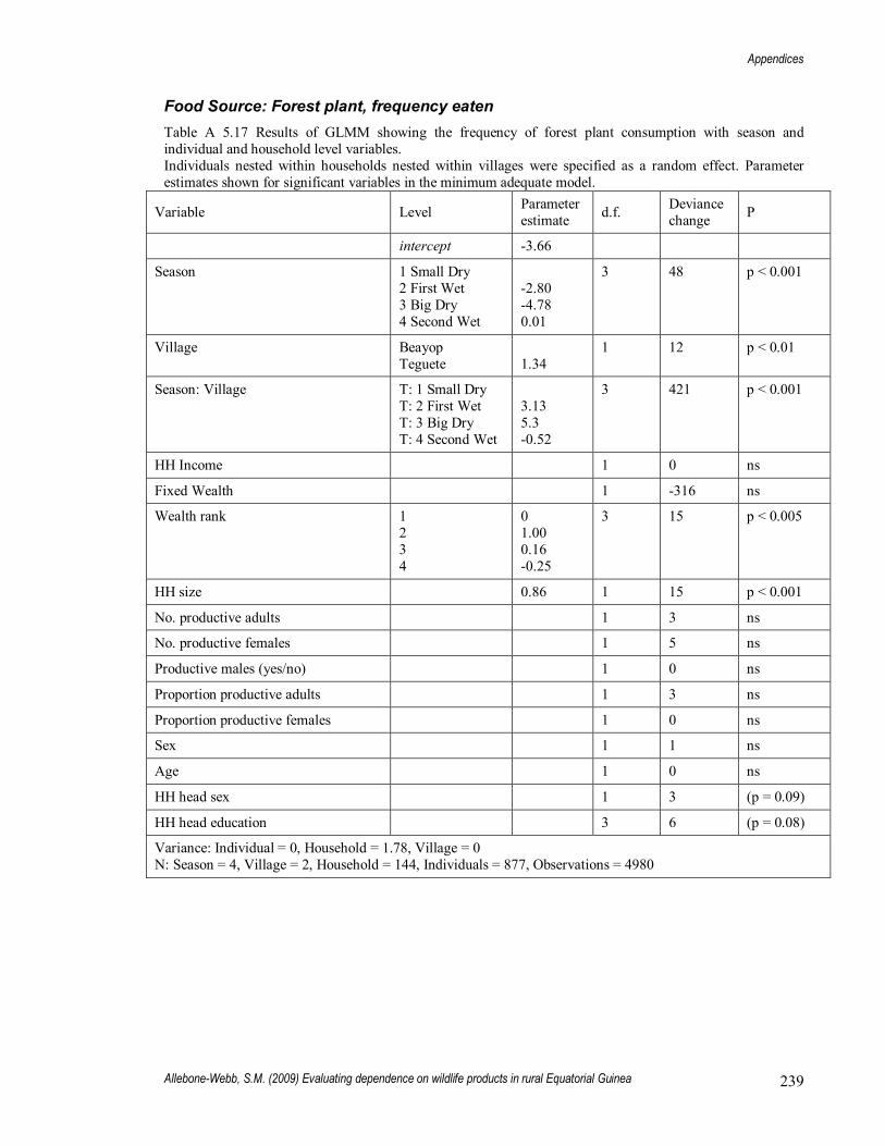
Appendices
Allebone-Webb, S.M. (2009) Evaluating dependence on wildlife products in rural Equatorial Guinea 239
Food Source: Forest plant, frequency eaten Table A 5.17 Results of GLMM showing the frequency of forest plant consumption with season and individual and household level variables. Individuals nested within households nested within villages were specified as a random effect. Parameter estimates shown for significant variables in the minimum adequate model.
Variable Level Parameter estimate d.f. Deviance
change P
intercept -3.66
Season 1 Small Dry 2 First Wet 3 Big Dry 4 Second Wet
-2.80 -4.78 0.01
3 48 p < 0.001
Village Beayop Teguete
1.34
1 12 p < 0.01
Season: Village T: 1 Small Dry T: 2 First Wet T: 3 Big Dry T: 4 Second Wet
3.13 5.3 -0.52
3 421 p < 0.001
HH Income 1 0 ns
Fixed Wealth 1 -316 ns
Wealth rank 1 2 3 4
0 1.00 0.16 -0.25
3 15 p < 0.005
HH size 0.86 1 15 p < 0.001
No. productive adults 1 3 ns
No. productive females 1 5 ns
Productive males (yes/no) 1 0 ns
Proportion productive adults 1 3 ns
Proportion productive females 1 0 ns
Sex 1 1 ns
Age 1 0 ns
HH head sex 1 3 (p = 0.09)
HH head education 3 6 (p = 0.08)
Variance: Individual = 0, Household = 1.78, Village = 0 N: Season = 4, Village = 2, Household = 144, Individuals = 877, Observations = 4980

Appendices
Allebone-Webb, S.M. (2009) Evaluating dependence on wildlife products in rural Equatorial Guinea 240
Food Type: Agriculture, proportion calories Table A 5.18 Results of LMM showing the correlation of proportion of calories consumed from agricultural food types with season and individual and household level variables. The arc-sin of the proportion of calories was taken to give a normal distribution. Individuals nested within households nested within villages were specified as a random effect. Parameter estimates shown for significant variables in the minimum adequate model.
Variable Level Parameter estimate d.f. Deviance
change P
Intercept 1.21
Season 1 Small Dry 2 First Wet 3 Big Dry 4 Second Wet
0 -0.091 -0.025 -0.055
3 19 p < 0.0001
Village Beayop Teguete
0.070
1 5 p < 0.05
Season: Village T: 1 Small Dry T: 2 First Wet T: 3 Big Dry T: 4 Second Wet
0.042 -0.014 0.14
3 19 p < 0.001
HH Income -0.029 1 4 p < 0.0001
Fixed Wealth 1 1 ns
Wealth rank 1 2 3 4 5
0 -0.01 -0.02 -0.12 -0.16
1 11 p < 0.05
HH size 1 1 ns
No. productive adults 1 1 ns
No. productive females 1 0 ns
Productive males (yes/no) 1 1 ns
Proportion productive adults 1 0 ns
Proportion productive females 1 0 ns
Sex 1 0 ns
Age 1 2 ns
HH head sex 1 0 ns
HH head education 3 6 ns
Variance: Individual = 0, Household = 0.024, Village = 0.00012, residual variance = 0.12 N: Season = 4, Village = 2, Household = 144, Individuals = 877, Observations = 4980

Appendices
Allebone-Webb, S.M. (2009) Evaluating dependence on wildlife products in rural Equatorial Guinea 241
Food Type: Agriculture, proportion protein Table A 5.19 Results of LMM showing the correlation of proportion of calories consumed from agricultural food types with season and individual and household level variables. The arc-sin of the proportion of calories was taken to give a normal distribution. Individuals nested within households nested within villages were specified as a random effect. Parameter estimates shown for significant variables in the minimum adequate model.
Variable Level Parameter estimate d.f. Deviance
change P
Intercept 1.01
Season 1 Small Dry 2 First Wet 3 Big Dry 4 Second Wet
0 -0.05 -0.02 -0.03
3 29 p < 0.0001
Village Beayop Teguete
0.15
1 5 p < 0.05
Season: Village T: 1 Small Dry T: 2 First Wet T: 3 Big Dry T: 4 Second Wet
-0.02 -0.1 0.11
3 33 p < 0.0001
HH Income -0.04 1 5 p < 0.05
Fixed Wealth 1 2 ns
Wealth rank 1 2 3 4 5
0 -0.05 -0.06 -0.16 -0.15
1 8 p < 0.05
HH size 1 1 ns
No. productive adults 1 0 ns
No. productive females 1 0 ns
Productive males (yes/no) 1 3 ns
Proportion productive adults 1 1 ns
Proportion productive females 1 1 ns
Sex 1 1 ns
Age 1 3 (p = 0.09)
HH head sex 1 0 ns
HH head education 3 3 ns
Variance: Individual = 0, Household = 0.029, Village = 3.4 e-7, residual variance = 0.14 N: Season = 4, Village = 2, Household = 144, Individuals = 877, Observations = 4980
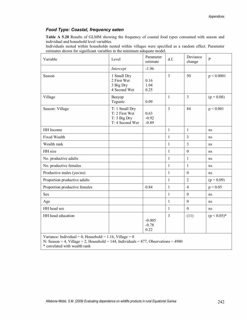
Appendices
Allebone-Webb, S.M. (2009) Evaluating dependence on wildlife products in rural Equatorial Guinea 242
Food Type: Coastal, frequency eaten Table A 5.20 Results of GLMM showing the frequency of coastal food types consumed with season and individual and household level variables. Individuals nested within households nested within villages were specified as a random effect. Parameter estimates shown for significant variables in the minimum adequate model.
Variable Level Parameter estimate d.f. Deviance
change P
Intercept -1.96
Season 1 Small Dry 2 First Wet 3 Big Dry 4 Second Wet
0.16 1.04 0.25
3 50 p < 0.0001
Village Beayop Teguete
0.09
1 3 (p = 0.08)
Season: Village T: 1 Small Dry T: 2 First Wet T: 3 Big Dry T: 4 Second Wet
0.63 -0.92 -0.89
3 84 p < 0.001
HH Income 1 1 ns
Fixed Wealth 1 3 ns
Wealth rank 1 3 ns
HH size 1 0 ns
No. productive adults 1 1 ns
No. productive females 1 1 ns
Productive males (yes/no) 1 0 ns
Proportion productive adults 1 2 (p = 0.09)
Proportion productive females 0.84 1 4 p < 0.05
Sex 1 0 ns
Age 1 0 ns
HH head sex 1 0 ns
HH head education -0.005 -0.78 0.22
3 (11) (p < 0.05)*
Variance: Individual = 0, Household = 1.16, Village = 0 N: Season = 4, Village = 2, Household = 144, Individuals = 877, Observations = 4980 * correlated with wealth rank

Appendices
Allebone-Webb, S.M. (2009) Evaluating dependence on wildlife products in rural Equatorial Guinea 243
Food Type: Coastal, proportion protein Table A 5.21 Results of LMM showing the correlation of proportion of protein consumed from coastal food types with season and individual and household level variables. The arc-sin of the proportion of protein was taken to give a normal distribution. Individuals nested within households nested within villages were specified as a random effect. Parameter estimates shown for significant variables in the minimum adequate model.
Variable Level Parameter estimate d.f. Deviance
change P
Intercept 0.35
Season 1 Small Dry 2 First Wet 3 Big Dry 4 Second Wet
-0.02 -0.04 -0.16
3 59 p < 0.001
Village Beayop Teguete
-0.23
1 6 p < 0.05
Season: Village T: 1 Small Dry T: 2 First Wet T: 3 Big Dry T: 4 Second Wet
0.06 0.12 0.12
3 40 p < 0.001
HH Income 1 2 ns
Fixed Wealth 1 1 ns
Wealth rank 1 2 3 4 5
0.06 0.12 0.12 0.15
1 13 p < 0.01
HH size 1 1 ns
No. productive adults 1 0 ns
No. productive females -0.18 1 19 p < 0.001
Productive males (yes/no) 1 3 ns
Proportion productive adults 1 1 ns
Proportion productive females 0.28 1 14 p < 0.01
Sex 1 0 ns
Age 1 0 ns
HH head sex 1 0 ns
HH head education 3 3 ns
Variance: Individual = 0, Household = 1.18, Village = 4 e-8 , 0.022 N: Season = 4, Village = 2, Household = 128, Individuals = 686, Observations = 1532

Appendices
Allebone-Webb, S.M. (2009) Evaluating dependence on wildlife products in rural Equatorial Guinea 244
Food Type: Import, frequency eaten Table A 5.22 Results of GLMM showing the frequency of imported food consumption with season and individual and household level variables. Individuals nested within households nested within villages were specified as a random effect. Parameter estimates shown for significant variables in the minimum adequate model.
Variable Level Parameter estimate d.f. Deviance
change P
Intercept -2.11
Season 1 Small Dry 2 First Wet 3 Big Dry 4 Second Wet
-0.737 -0.86 0.15
3 15 p < 0.005
Village Beayop Teguete
-1.37
1 8 p < 0.005
HH Income 0.26 1 7 p < 0.01
Fixed Wealth 1 -395 ns
Wealth rank 1 4 ns
HH size 1 0 ns
No. productive adults 1 0 ns
No. productive females 1 1 ns
Productive males (yes/no) 1 2 ns
Proportion productive adults 1 0 ns
Proportion productive females 1 1 ns
Sex 1 0 ns
Age 1 0 ns
Education 1 ns
HH head sex 1 1 ns
HH head education None Primary Secondary Higher
0.11 1.00 1.06
3 12 p < 0.01
Variance: Individual = 0, Household = 1.11, Village = 0 N: Season = 4, Village = 2, Household = 145, Individuals = 932, Observations = 5129

Appendices
Allebone-Webb, S.M. (2009) Evaluating dependence on wildlife products in rural Equatorial Guinea 245
Food Type: Wild (all), frequency eaten Table A 5.23 Results of GLMM showing the frequency of wild food consumption with season and individual and household level variables. Individuals nested within households nested within villages were specified as a random effect. Parameter estimates shown for significant variables in the minimum adequate model.
Variable Level Parameter estimate d.f. Deviance
change P
Intercept -1.71
Season 1 Small Dry 2 First Wet 3 Big Dry 4 Second Wet
0 -0.35 -0.25 -0.45
3 40 p < 0.001
Village Beayop Teguete
1.19
1 10 p < 0.001
Season: Village T: 1 Small Dry T: 2 First Wet T: 3 Big Dry T: 4 Second Wet
1.16 0.88 -0.28
3 43 p < 0.001
HH Income 1 0 ns
Fixed Wealth 1 -280 ns
Wealth rank 1 2 3 4
0 -0.3 -0.70 -0.01
1 10 p < 0.05
HH size 0.65 1 18 ns
No. productive adults 1 0 ns
No. productive females 1 0 ns
Productive males (yes/no) 1 0 ns
Proportion productive adults 1 0 ns
Proportion productive females 1 0 ns
Sex 1 1 ns
Age 1 0 ns
HH head sex 1 0 ns
HH head education 3 3 ns
Variance: Individual = 0, Household = 0.85, Village = 0 N: Season = 4, Village = 2, Household = 144, Individuals = 877, Observations = 4980

Appendices
Allebone-Webb, S.M. (2009) Evaluating dependence on wildlife products in rural Equatorial Guinea 246
Food Type: Wild (all), proportion protein Table A 5.24 Results of LMM showing the correlation of proportion of protein consumed from wild food types with season and individual and household level variables. The arc-sin of the proportion of protein was taken to give a normal distribution. Individuals nested within households nested within villages were specified as a random effect. Parameter estimates shown for significant variables in the minimum adequate model.
Variable Level Parameter estimate d.f. Deviance
change P
Intercept 0.45
Season 1 Small Dry 2 First Wet 3 Big Dry 4 Second Wet
0 -0.002 0.076 0.028
3 32 p < 0.0001
Village Beayop Teguete
0 0.07
1 4 p < 0.05
HH Income 1 1 ns
Fixed Wealth 1 0 ns
Wealth rank 1 3 ns
HH size 1 1 ns
No. productive adults 1 0 ns
No. productive females 1 0 ns
Productive males (yes/no) 1 0 ns
Proportion productive adults 1 0 ns
Proportion productive females 1 2 ns
Sex 1 1 ns
Age 1 0 ns
HH head sex 1 2 ns
HH head education 3 1 ns
Variance: Individual = 6 e-17, Household = 0.03, Village = 0 , residual variance = 0.11 N: Season = 4, Village = 2, Household = 138, Individuals = 776, Observations = 2794
Food Type: Wild (all), proportion calories Table A 5.25 Results of LMM showing the correlation of proportion of calories consumed from wild food types with season and individual and household level variables. The arc-sin of the proportion of calories was taken to give a normal distribution. Individuals nested within households nested within villages were specified as a random effect. Parameter estimates shown for significant variables in the minimum adequate model.
Variable Level Parameter estimate d.f. Deviance
change P
Intercept 0.28
Season 1 Small Dry 2 First Wet 3 Big Dry 4 Second Wet
0 -0.03 -0.05 -0.08
3 49 p < 0.0001

Appendices
Allebone-Webb, S.M. (2009) Evaluating dependence on wildlife products in rural Equatorial Guinea 247
Village Beayop Teguete
-0.008
1 7 p < 0.01
Season: Village T: 1 Small Dry T: 2 First Wet T: 3 Big Dry T: 4 Second Wet
0.11 0.11 0.04
3 36 p < 0.001
HH Income 1 1 ns
Fixed Wealth 1 2 ns
Wealth rank 1 0 ns
HH size 1 5 (p < 0.05)
No. productive adults 1 4 (p = 0.06)
No. productive females -0.05 1 8 p < 0.01
Productive males (yes/no) 1 0 ns
Proportion productive adults 1 0 ns
Proportion productive females 1 2 ns
Sex 1 0 ns
Age 1 0 ns
HH head sex 1 0 ns
HH head education 3 0 ns
Variance: Individual = 6 e-17, Household = 0.007, Village = 0, residual variance = 0.022 N: Season = 4, Village = 2, Household = 138, Individuals = 776, Observations = 2794
Food Type: Wild animal, frequency eaten Table A 5.26 Results of GLMM showing the frequency of wild animal consumption with season and individual and household level variables. Individuals nested within households nested within villages were specified as a random effect. Parameter estimates shown for significant variables in the minimum adequate model.
Variable Level Parameter estimate d.f. Deviance
change P
Intercept -4.0
Season 1 Small Dry 2 First Wet 3 Big Dry 4 Second Wet
0 -0.53 -0.45 -1.0
3 50 p < 0.001
Village Beayop Teguete
1.46
1 10 p < 0.01
Season: Village T: 1 Small Dry T: 2 First Wet T: 3 Big Dry T: 4 Second Wet
-0.06 0.75 1.20
3 27 p < 0.001
HH Income 1 2 ns
Fixed Wealth 1 -4 ns
Wealth rank 1 1 ns

Appendices
Allebone-Webb, S.M. (2009) Evaluating dependence on wildlife products in rural Equatorial Guinea 248
HH size 0.79 1 17 p < 0.001
No. productive adults 1 4 ns
No. productive females 1 3 ns
Productive males (yes/no) 1 0 ns
Proportion productive adults 1 1 ns
Proportion productive females 1 1 ns
Sex 1 1 ns
Age 1 0 ns
HH head sex 1 0 ns
HH head education 3 6 ns
Variance: Individual = 6 e-17, Household = 1.46, Village = 0 N: Season = 4, Village = 2, Household = 144, Individuals = 877, Observations = 4980
Food Type: Wild animal, proportion protein Table A 5.27 Results of LMM showing the correlation of proportion of protein consumed from wild animal with season and individual and household level variables. The arc-sin of the proportion of protein was taken to give a normal distribution. Individuals nested within households nested within villages were specified as a random effect. Parameter estimates shown for significant variables in the minimum adequate model.
Variable Level Parameter estimate d.f. Deviance
change P
Intercept 0.76
Season 1 Small Dry 2 First Wet 3 Big Dry 4 Second Wet
0 0.10 -0.05 -0.26
3 48 p < 0.001
Village Beayop Teguete
-0.13
1 1 ns
Season: Village T: 1 Small Dry T: 2 First Wet T: 3 Big Dry T: 4 Second Wet
-0.01 0.16 0.17
3 16 p < 0.01
HH Income (+) 1 4 (p = 0.054)
Fixed Wealth 1 0 ns
Wealth rank 1 1 ns
HH size 1 0 ns
No. productive adults 1 1 ns
No. productive females 1 2 ns
Productive males (yes/no) 1 0 ns
Proportion productive adults 1 1 ns
Proportion productive females 1 1 ns

Appendices
Allebone-Webb, S.M. (2009) Evaluating dependence on wildlife products in rural Equatorial Guinea 249
Sex 1 0 ns
Age 1 0 ns
HH head sex 1 0 ns
HH head education 3 3 ns
Variance: Individual = 2.5 e-17, Household = 0.04, Village = 3.8 e -8 , residual = 0.065 N: Season = 4, Village = 2, Household = 107, Individuals = 577, Observations = 1358
Food Type: Wild Fish, frequency eaten Table A 5.28 Results of GLMM showing the frequency of wild fish consumption with season and individual and household level variables. Individuals nested within households nested within villages were specified as a random effect. Parameter estimates shown for significant variables in the minimum adequate model.
Variable Level Parameter estimate d.f. Deviance
change P
Intercept -3.22
Season 1 Small Dry 2 First Wet 3 Big Dry 4 Second Wet
0 0.81 1.20 1.32
3 0
Village Beayop Teguete
1.28
1 1
Season: Village T: 1 Small Dry T: 2 First Wet T: 3 Big Dry T: 4 Second Wet
-1.12 -1.19 -2.65
3 62 p < 0.0001
HH Income 1 1 ns
Fixed Wealth 1 1 ns
Wealth rank 1 4 ns
HH size 1 0 ns
No. productive adults 1 1 ns
No. productive females 1 -2 ns
Productive males (yes/no) 1 1 ns
Proportion productive adults 1 1 ns
Proportion productive females 1 1 ns
Sex 1 0 ns
Age 1 1 ns
HH head sex 1 1 ns
HH head education 3 6 ns
Variance: Individual = 5 e-10, Household = 1.87, Village = 5 e -10 N: Season = 4, Village = 2, Household = 144, Individuals = 877, Observations = 4980

Appendices
Allebone-Webb, S.M. (2009) Evaluating dependence on wildlife products in rural Equatorial Guinea 250
Food Type: Wild fish, proportion protein Table A 5.29 Results of LMM showing the correlation of proportion of protein consumed from wild fish with season and individual and household level variables. The arc-sin of the proportion of protein was taken to give a normal distribution. Individuals nested within households nested within villages were specified as a random effect. Parameter estimates shown for significant variables in the minimum adequate model.
Variable Level Parameter estimate d.f. Deviance
change P
Intercept 0.75
Season 1 Small Dry 2 First Wet 3 Big Dry 4 Second Wet
0 -0.08 -0.01 0.08
3 49 p < 0.001
Village Beayop Teguete
-0.35
1 7 p < 0.01
Season: Village T: 1 Small Dry T: 2 First Wet T: 3 Big Dry T: 4 Second Wet
0.31 0.12 0.31
3 50 p < 0.001
HH Income -0.025 1 4 p 0.05
Fixed Wealth 1 0 ns
Wealth rank 1 5 ns
HH size 1 2 ns
No. productive adults 1 0 ns
No. productive females 1 0 ns
Productive males (yes/no) 1 1 ns
Proportion productive adults 1 1 ns
Proportion productive females 1 2 ns
Sex 1 1 ns
Age 1 1 ns
HH head sex 1 0 ns
HH head education 3 7 ns
Variance: Individual = 0, Household = 0.25, Village = 0, residual = 0.024 N: Season = 4, Village = 2, Household = 92, Individuals = 495, Observations = 809

Appendices
Allebone-Webb, S.M. (2009) Evaluating dependence on wildlife products in rural Equatorial Guinea 251
Food Type: Wild plant, frequency eaten Table A 5.30 Results of GLMM showing the frequency of wild plant consumption with season and individual and household level variables. Individuals nested within households nested within villages were specified as a random effect. Parameter estimates shown for significant variables in the minimum adequate model.
Variable Level Parameter estimate d.f. Deviance
change P
Intercept -2.0
Season 1 Small Dry 2 First Wet 3 Big Dry 4 Second Wet
-0.91 -1.23 -1.84
3 148 p < 0.001
Village Beayop Teguete
1.98
1 11 p < 0.001
Season: Village T: 1 Small Dry T: 2 First Wet T: 3 Big Dry T: 4 Second Wet
1.77 1.74 -0.16
3 69 p < 0.001
HH Income 1 1 ns
Fixed Wealth 1 -30 ns
Wealth rank 1 2 3 4
0.24 0.96 0.86
2 ns
Wealth rank : Village T : 1 T : 2 T : 3 T : 4
-0.18 -1.76 -0.91
10 p < 0.05
HH size 1 4 ns
No. productive adults 1 0 ns
No. productive females 1 0 ns
Productive males (yes/no) 1 1 ns
Proportion productive adults 1 2 ns
Proportion productive females 1 2 ns
Sex 1 0 ns
Age 1 1 ns
HH head sex 1 1 ns
HH head education 3 7 (p = 0.08)
Variance: Individual = 5 e -10, Household = 1.16, Village = 5 e --10, N: Season = 4, Village = 2, Household = 144, Individuals = 877, Observations = 4980

Appendices
Allebone-Webb, S.M. (2009) Evaluating dependence on wildlife products in rural Equatorial Guinea 252
Food Type: Wild plant, proportion calories Table A 5.31 Results of LMM showing the correlation of proportion of calories consumed from wild plants with season and individual and household level variables. The arc-sin of the proportion of calories was taken to give a normal distribution. Individuals nested within households nested within villages were specified as a random effect. Parameter estimates shown for significant variables in the minimum adequate model
Variable Level Parameter estimate d.f. Deviance
change P
Intercept 0.32
Season 1 Small Dry 2 First Wet 3 Big Dry 4 Second Wet
0.007 -0.015 0.05
3 191 0.01
Village Beayop Teguete
0.009
1 25 p < 0.05
Season: Village T: 1 Small Dry T: 2 First Wet T: 3 Big Dry T: 4 Second Wet
0.10 0.05 -0.08
3 23 p < 0.001
Money (-0.013) 1 7 p = 0.058
Fixed Wealth 1 1 ns
Wealth rank 4 1 ns
HH size -0.06 1 28 p < 0.001
No. productive adults 1 8 (p < 0.01)
No. productive females 1 14 (p < 0.001)
Productive males (yes/no) 1 0 ns
Proportion productive adults 1 3 ns
Proportion productive females 1 0 ns
Sex 1 0 ns
Age 1 0 ns
HH head sex 1 0 ns
HH head education 3 3 ns
Variance: Individual = 0, Household = 0.005, Village = 0, residual = 0.009 N: Season = 4, Village = 2, Household = 122, Individuals = 603, Observations = 1720

Appendices
Allebone-Webb, S.M. (2009) Evaluating dependence on wildlife products in rural Equatorial Guinea 253
Appendix 6. Supplementary material: Chapter 4
Table A 6.1 Results from LMM � total household production value/household total AME. HH Income not analysed.
Variable d.f. Parameter estimate
d.f. Deviance change
P
intercept -5.42 Season 1 Small Dry
2 First Wet 3 Big Dry 4 Second Wet
-0.90 0.37 -0.25
3 44 p < 0.0001
Village Beayop Teguete
0.55
1 1 ns
Village:Season T: 1 Small Dry T: 2 First Wet T: 3 Big Dry T: 4 Second Wet
-1.25 -1.68 -0.61
1 15 p < 0.01
Fixed Wealth 0.71 1 11 p < 0.0001 Wealth rank 1 2 ns HH size 1 0 ns No. productive adults 1 0 ns No. productive females 1 0 ns Productive males (yes/no) 1 1 ns Proportion productive adults 1 3 ns Proportion productive females 1.05 1 6 p < 0.05 HH head sex Female
Male 0.61
1 8 p < 0.01
HH head education 3 3 ns Variance: HH = 0.54, Village = 0.036, Residual = 3.49 n (HH) = 147, n (observations) = 521
Table A 6.2 Results from GLMM - Likelihood of a household earning money in a particular season
Variable d.f. Parameter estimate
d.f. Deviance change
P
intercept -12.77 Season 1 Small Dry
2 First Wet 3 Big Dry 4 Second Wet
-1.10 -0.04 -0.53
3 19.3 p < 0.001
Village 1 0 ns Fixed Wealth 0.77 1 11 p < 0.05 Wealth rank 1
2 3 4
0.72 0.52 1.35
1 11 p < 0.05
HH size 0.65 1 9 p < 0.01 No. productive adults 1 8 ns

Appendices
Allebone-Webb, S.M. (2009) Evaluating dependence on wildlife products in rural Equatorial Guinea 254
No. productive females 1 6 ns Productive males (yes/no) 1 2.4 ns Proportion productive adults 1 0.3 ns Proportion productive females 1 0.1 ns HH head sex Female
Male 0.66
1 7 p < 0.01
HH head education 3 2.2 ns Variance: HH = 0.0.46, Village = 0 n (HH) = 147, n (observations) = 521
Table A 6.3 Results from LMM � Amount earned per HH per AME (earners only)
Variable d.f. Parameter estimate
d.f. Deviance change
P
intercept 7.53 Season 3 0.6 ns Village Beayop
Teguete -0.81
1 5.2 p < 0.05
Fixed Wealth 1 3.8 p = 0.052 Wealth rank 1
2 3 4
0 -0.49 0.04
1 10 p < 0.05
HH size -0.68 1 21 p < 0.001 No. productive adults 1 5.5 ns No. productive females 1 7 ns Productive males (yes/no) 1 0 ns Proportion productive adults 1 6 ns Proportion productive females 1 1 ns HH head sex Female
Male -0.39
1 5.4 p < 0.05
HH head education None Primary Secondary Higher
0.43 0.97 0.27
3 13 p < 0.01
Table A 6.4. Results from LMM � likelihood of production, all forest products (>18)
Variable d.f. Parameter estimate
d.f. Deviance change
P
intercept -1.06 Season 1 Small Dry
2 First Wet 3 Big Dry 4 Second Wet
-1.49 -0.63 -0.84
3 48 p < 0.0001
Village Beayop Teguete
1 1 ns
Gun (yes/no) (only 6 HHs) 1 1 ns HH Income -0.06 1 0 ns

Appendices
Allebone-Webb, S.M. (2009) Evaluating dependence on wildlife products in rural Equatorial Guinea 255
Sex Female Male
-3.08
1 15
p < 0.001
HH Income: Sex Income: Female Income: Male
0.29
1 14 p < 0.05
Fixed Wealth 1 ns Wealth rank 1 5 ns HH size (sqrt) 1 0 ns No. productive adults 1 0 ns No. productive females 1 0 ns Productive males (yes/no) 1 2 ns Dependence prop (adult) 1 0 ns Dependence prop (female) 1 2 ns Age 18 � 30
30 � 50 50 � 65 65+
1.05 1.19 0.78
1 19 p < 0.0001
Education 3 7 ns HH head sex 1 0 ns HH head education 3 6 (p = 0.08) Variance: Individual = 0.46, HH = 0.031, Village = 0 n (Village) = 2, n (HH) = 152, n (individual) = 1348, n (observations) = 1348
Table A 6.5. Results from LMM � (log) value of all forest products (>18, producers only)
Variable d.f. Parameter estimate
d.f. Deviance change
P
intercept 6.04 Season 1 Small Dry
2 First Wet 3 Big Dry 4 Second Wet
-0.09 -0.90 -0.22
3 24 p < 0.0001
Village Beayop Teguete
1.93
1 6 p < 0.05
Gun (yes/no) (only 6 HHs) 1 ns Chainsaw (yes/no) (only 10 HHs) 1 ns HH Income 1 0 ns Fixed Wealth 1 ns Wealth rank 1
2 3 4
-0.18 -0.57 -0.08
3 8 p < 0.05
HH size (sqrt) 1 0 ns No. productive adults 1 0 ns No. productive females 1 0 ns Productive males (yes/no) 1 1 ns Dependence prop (adult) 1 0 ns Dependence prop (female) 1 0 ns

Appendices
Allebone-Webb, S.M. (2009) Evaluating dependence on wildlife products in rural Equatorial Guinea 256
Sex Female Male
3.04
1 83 p < 0.0001
Village: Sex T: Female T: Male
-2.19
47 p < 0.001
Age -0.19 1 7 p < 0.01 Education 3 3 ns HH head sex 1 0 ns HH head education 3 3 ns Variance: Individual = 0, HH = 0.043, Village = 0, Residual variance = 0.021 n: Village = 2, HH = 119, Individual = 206, Observations = 289
Table A 6.6 Likelihood of income from all forest products (>18)
Variable Parameter estimate
d.f. Deviance change
P
intercept -5.31
Season 1 Small Dry 2 First Wet 3 Big Dry 4 Second Wet
-0.40 0.36 -0.68
3 8.3 p < 0.05
Village Beayop Teguete
0.81
1 4.8 p < 0.05
HH Income 3 3.7 p = 0.056
HH Fixed Wealth 1 ns
HH Wealth rank 1 2.3 ns
HH size 1 0.1 ns
No. productive adults 1 0 ns
No. productive females 1 0.2 ns
Productive males (yes/no) 1 0.5 ns
Proportion productive adults 1 0.1 ns
Proportion productive females 1 0.5 ns
HH head education 3 3.3 ns
HH head sex 1 0.3 ns
Sex Female Male
1.77
1 16 p < 0.0001
Age 1 2.1 ns
Education 3 3.2 ns
Variance : Individual = 2.54, HH = 0, Village = 0 n: Village = 2, HH = 152, Individual = 473, observations = 1348

Appendices
Allebone-Webb, S.M. (2009) Evaluating dependence on wildlife products in rural Equatorial Guinea 257
Table A 6.7 Amount of income from all forest products (>18). Age (categorical) also significant, but not significantly different from Age (continuous).
Variable Parameter estimate
d.f. Deviance change
P
intercept 2.87
Season 1 Small Dry 2 First Wet 3 Big Dry 4 Second Wet
3 3.5 ns
Village Beayop Teguete
1 0.6 ns
HH Income 0.47 3 9.3 p < 0.01
HH Fixed Wealth 1 ns
HH Wealth rank 1 1.7 ns
HH size 1 0.1 ns
No. productive adults 1 0.1 ns
No. productive females 1 0 ns
Productive males (yes/no) 1 0.8 ns
Proportion productive adults 1 0.1 ns
Proportion productive females 1 0.3 ns
HH head education 3 1.2 ns
HH head sex 1 1.6 ns
Sex Female Male
1 5.1 p = 0.079
Age -0.32 1 10.5 p < 0.01
Education 3 1 ns
Variance : Individual = 0.067, HH = 2.3 e -9, Village = 0.033, Residual = 0.78 n: Village = 2, HH = 49, Individual = 59, observations = 68
Table A 6.8. Results from GLMM � likelihood of production forest animals (>18)
Variable Parameter estimate
d.f. Deviance change
P
intercept -8.85
Season 1 Small Dry 2 First Wet 3 Big Dry 4 Second Wet
-0.32 1.29 -1.44
3 14 p < 0.001
Village 1 1 ns
HH Income (log) 1 1 ns
HH Fixed Wealth (sqrt) 1 ns
HH Wealth rank 3 7 ns
HH size (sqrt) 1 1 ns

Appendices
Allebone-Webb, S.M. (2009) Evaluating dependence on wildlife products in rural Equatorial Guinea 258
No. productive adults (sqrt) 1 0 ns
No. productive females (sqrt) 1 1 ns
Productive males (yes/no) 1 4 p = 0.07
Dependence prop (adult) (sqrt(asin()) 1 2 ns
Dependence prop (female) (sqrt(asin()) 1 0 ns
HH head sex 1 0 ns
HH head education 3 1 ns
HH Gun (yes/no) (only 8 HHs) 1 0 ns
Sex Female Male
3.27
1 14 p < 0.001
Age (sqrt) 1 3 ns
Education (higher education = lower hunting)
3 7 p = 0.06
Variance : Individual = 0.20, HH = 0, Village = 0 n: Village = 2, HH = 141, Individual = 382, observations = 1053
Table A 6.9. Results from mixed model � value of production, forest animals (only producers > 18)
Variable (value logged)
Parameter estimate
d.f. Deviance change
P
intercept 2.96
Season 1 Small Dry 2 First Wet 3 Big Dry 4 Second Wet
-0.05 -1.16 -0.45
3 20 p < 0.0001
Village 1 2 ns
HH Income (log) 0.30 1 6 p < 0.05
HH Fixed Wealth (sqrt) 1 ns
HH Wealth rank 1 4 ns
HH size (sqrt) 1 0 ns
No. productive adults (sqrt) 1 0 ns
No. productive females (sqrt) 1 3 ns
Productive males (yes/no) 1 1 ns
Dependence prop (adult) (sqrt(asin()) 1 0 ns
Dependence prop (female) (sqrt(asin()) 1 2 ns
HH head sex 1 1 ns
HH head education 3 0 ns
HH Gun (yes/no) (only 8 HH owned a gun)
1 2 ns
Sex Female Male
1.09
1 10 p < 0.01

Appendices
Allebone-Webb, S.M. (2009) Evaluating dependence on wildlife products in rural Equatorial Guinea 259
Age (sqrt) 1 1 ns
Education 1* 2 ns
Variance : Individual = 0, HH = 0, Village = 0 n: Village = 2, HH = 51, Individual = 61, observations = 82 * only people with primary or secondary education gained value from forest animals (none with no education or higher education)
Table A 6.10. Results from GLMM � likelihood of production forest fish (>18)
Variable Parameter estimate
d.f. Deviance change
P
intercept -8.78
Season 3 7 p = 0.07
Village 1 0 ns
HH Income (log) 1 0 ns
HH Fixed Wealth (sqrt) 1 0 ns
HH Wealth rank 3 2 ns
HH size (sqrt) 1 0 ns
No. productive adults (sqrt) 1 0 ns
No. productive females (sqrt) 1 0 ns
Productive males (yes/no) 1 0 ns
Dependence prop (adult) (sqrt(asin()) 1 0 ns
Dependence prop (female) (sqrt(asin()) 1 0 ns
HH head sex 1 0 ns
HH head education 3 0 ns
Sex 1 0 ns
Age 1 1 ns
Education 3 1.5 ns
Variance : Individual = 5.69, HH = 0, Village = 0 n: Village = 2, HH = 141, Individual = 382, observations = 1053
Table A 6.11. Results from GLMM � likelihood of production forest plants (>18)
Variable Parameter estimate
d.f. Deviance change
P
intercept 0.91
Season 1 Small Dry 2 First Wet 3 Big Dry 4 Second Wet
-0.89 0.75 0.50
3 33 p < 0.0001
Village Beayop Teguete
1.40
1 0

Appendices
Allebone-Webb, S.M. (2009) Evaluating dependence on wildlife products in rural Equatorial Guinea 260
Season: Village T: 1 Small Dry T: 2 First Wet T: 3 Big Dry T: 4 Second Wet
-1.85 -3.01 -1.44
3 25 p < 0.0001
HH Income 3 0 ns
HH Fixed Wealth 1 ns
HH Wealth rank 1 4 ns
HH size (sqrt) 1 1 ns
No. productive adults 1 0 ns
No. productive females 1 1 ns
Productive males (yes/no) 1 0 ns
Proportion productive adults 1 0 ns
Proportion productive females 1 0 ns
HH head education 3 8 (p = 0.051)
HH head sex 1 0 ns
Sex 1 2 ns
Age 0.62 1 28 p < 0.0001
Education 3 0 ns
Variance : Individual = 0.20, HH = 0, Village = 0 n: Village = 2, HH = 141, Individual = 382, observations = 1053
Table A 6.12. Results from GLMM � value of production forest plants (>18)
Variable Parameter estimate
d.f. Deviance change
P
intercept 4.25
Season 1 Small Dry 2 First Wet 3 Big Dry 4 Second Wet
1.16 -0.43 0.33
3 30 p < 0.0001
Village Beayop Teguete
2.93
1 6 p < 0.01
Season: Village T: 1 Small Dry T: 2 First Wet T: 3 Big Dry T: 4 Second Wet
-2.74 -2.50 -1.92
3 26 p < 0.0001
HH Income 3 0 ns
HH Fixed Wealth 1 0 ns
HH Wealth rank 1 7 p = 0.07
HH size (sqrt) 1 0.5 ns
No. productive adults 1 0 ns
No. productive females 1 0.5 ns

Appendices
Allebone-Webb, S.M. (2009) Evaluating dependence on wildlife products in rural Equatorial Guinea 261
Productive males (yes/no) 1 2.5 p = 0.06
Proportion productive adults 1 0 ns
Proportion productive females 1 4 p = 0.055
HH head education 3 0 ns
HH head sex 1 5 ns
Sex Female Male
1.39
1 24 p < 0.0001
Age 1 0 ns
Education 3 5 ns
Variance : Individual = 0.20, HH = 0, Village = 0 n: Village = 2, HH = 141, Individual = 382, observations = 1053
Table A 6.13. Results from GLMM � likelihood of income from forest animals (>18)
Variable Parameter estimate
d.f. Deviance change
P
intercept -11.87
Season 1 Small Dry 2 First Wet 3 Big Dry 4 Second Wet
-0.38 0.55 -1.60
3 11 p < 0.01
Village Beayop Teguete
1.07
1 4 p > 0.05
HH Income 0.51 3 4 p > 0.05
HH Fixed Wealth 1 ns
HH Wealth rank 1 2 3 4
-0.25 -1.07 -2.15
1 10 p > 0.05
HH size (sqrt) 1 0 ns
No. productive adults 1 1 ns
No. productive females 1 0 ns
Productive males (yes/no) 1 4 ns
Proportion productive adults 1 1 ns
Proportion productive females 1 0 ns
HH head education 3 2 ns
HH head sex 1 2 ns
Sex Female Male
2.45
1 14 p < 0.001
Age 1 0 ns
Education 3 4 ns

Appendices
Allebone-Webb, S.M. (2009) Evaluating dependence on wildlife products in rural Equatorial Guinea 262
Variance : Individual = 0.20, HH = 0, Village = 0 n: Village = 2, HH = 141, Individual = 382, observations = 1053
Table A 6.14. Results from GLMM � amount income from forest animals (>18)
Variable Parameter estimate
d.f. Deviance change
P
intercept 1.39
Season 3 4.5 ns
Village 1 -2 ns
HH Income 0.45 3 5.5 p < 0.05
HH Fixed Wealth 1 3 ns
HH Wealth rank 1 4 ns
HH size (sqrt) 1 1 ns
No. productive adults 1 0 ns
No. productive females 1 0 ns
Productive males (yes/no) 1 1 ns
Proportion productive adults 1 2 ns
Proportion productive females 1 1 ns
HH head education 3 0 ns
HH head sex 1 3 (p = 0.09)
Sex 1 0 ns
Age 1 0 ns
Education 3 1 ns
Variance : Individual = 0, HH = 0, Village = 0, Residual variance = 0.52 n: Village = 2, HH = 32, Individual = 35, observations = 39
Table A 6.15. Results from GLMM � likelihood of income from forest plants (>18)
Variable Parameter estimate
d.f. Deviance change
P
intercept -9.53
Season 3 1 ns
Village 1 0 ns
HH Income 3 0 ns
HH Fixed Wealth 1 ns
HH Wealth rank 1 0 ns
HH size (sqrt) 1 0 ns
No. productive adults 1 0 ns
No. productive females 1 0 ns

Appendices
Allebone-Webb, S.M. (2009) Evaluating dependence on wildlife products in rural Equatorial Guinea 263
Productive males (yes/no) 1 0 ns
Proportion productive adults 1 0 ns
Proportion productive females 1 0 ns
HH head education 3 2 ns
HH head sex 1 2 ns
Sex 1 1.5 ns
Age 1 0 ns
Education 3 1 ns
Variance : Individual = 5.9, HH = 0, Village = 0 n: Village = 2, HH = 152, Individual = 473, observations = 1348
Figure A 6.1. Income from all people (18-65), average cfa per day (Beayop)
0
100
200
300
400
500
600
700
800
900
1000
1 2 3 4 1 2 3 4
Female Male
Beayop
Wealth rank and sex
Ave
rage
inco
me/
day
(cfa
), al
l peo
ple
(18-
65)
ForestPaidProducedTrade

Appendices
Allebone-Webb, S.M. (2009) Evaluating dependence on wildlife products in rural Equatorial Guinea 264
Figure A 6.2. Income from all people (18-65), average cfa per day (Teguete)
0
100
200
300
400
500
600
700
800
900
1000
1 2 3 4 1 2 3 4
Female Male
Teguete
Wealth rank and sex
Aver
age
inco
me/
day
(cfa
), al
l peo
ple
(18-
65)
ForestPaidProducedTrade
Figure A 6.3. Income from all sources, people earning from that income only (and in those seasons only), average cfa per day (Beayop), all ages
0
200
400
600
800
1000
1200
1400
1600
1800
2000
1 2 3 4 1 2 3 4
Female Male
Beayop
1
Wealth rank and sex
Ave
rage
val
ue/d
ay o
f goo
ds h
arve
sted
/pro
duce
d (c
fa),
all p
eopl
e (1
8-65
)
ForestPaidProducedTrade

Appendices
Allebone-Webb, S.M. (2009) Evaluating dependence on wildlife products in rural Equatorial Guinea 265
Figure A 6.4. Income from all sources, people earning from that income only (and in those seasons only), average cfa per day (Teguete), all ages
0
200
400
600
800
1000
1200
1400
1600
1800
2000
1 2 3 4 1 2 3 4
Female Male
Teguete
1
Wealth rank and sex
Ave
rage
val
ue/d
ay o
f goo
ds h
arve
sted
/pro
duce
d (c
fa),
all p
eopl
e (1
8-65
)
ForestPaidProducedTrade
Table A 6.16. Results from GLMM � likelihood of value for agricultural products (all people >18).
Age (categorical) is a significantly better fit than age as a continuous variable.
Variable Level Parameter estimate d.f. Deviance
change P
Intercept -1.25
Season 1 Small Dry 2 First Wet 3 Big Dry 4 Second Wet
-0.72 0.21 0.36
3 29 p < 0.0001
Village 1 0 ns
HH Income 3 0 ns
HH Fixed Wealth 1 ns
Wealth rank 3 7 p = 0.07
HH size 1 2 ns
No. productive adults 1 0 ns
No. productive females 1 1 ns
Productive males (yes/no) 1 1 ns
Proportion productive adults 1 2 ns
Proportion productive females 1 5 p = 0.052
HH head education 3 6 ns
HH head sex Female Male
0.57
1 10 p < 0.05

Appendices
Allebone-Webb, S.M. (2009) Evaluating dependence on wildlife products in rural Equatorial Guinea 266
Sex Female Male
-0.359
1 220 p < 0.0001
Age 18-30 30-50 50-65 65+
1.45 2.49 1.57
3 73 p < 0.0001
Education 3 4 ns
Variance: Individual = 1.25, Household = 0.093, Village = 0 N: Individual = 473, Household = 152, Village = 2, Observations = 1348
Table A 6.17. Results from LMM - value of all agricultural products
Variable Level Parameter estimate d.f. Deviance
change P
Intercept -0.71
Season 1 Small Dry 2 First Wet 3 Big Dry 4 Second Wet
-0.73 0.37 -0.04
3 43 p < 0.0001
Village Beayop Teguete
0.05
1 2 ns
Season: Village T: 1 Small Dry T: 2 First Wet T: 3 Big Dry T: 4 Second Wet
-0.53 -1.09 0.32
3 17 p < 0.001
Age 0.69 1 79 p < 0.0001
Sex Female Male
-15.5
1 181 p < 0.0001
Wealth rank 3 7 (p = 0.08)
Income 1 3 (p = 0.09)
HH Head Education 3 7 (p = 0.07)
Variance: Individual = 1.58, Household = 0.07, Village = 0.02, Residual variance = 4.65 N: Individual = 411, Household = 147, Village = 2, Observations = 1149 Table A 6.18. Results from GLMM � likelihood of income of all agricultural products
Variable Level Parameter estimate d.f. Deviance
change P
Intercept -3.41
Season 1 Small Dry 2 First Wet 3 Big Dry 4 Second Wet
-1.04 0.75 -0.62
3 16.7 p < 0.001
Village Beayop Teguete
-0.35
1 2.1 ns

Appendices
Allebone-Webb, S.M. (2009) Evaluating dependence on wildlife products in rural Equatorial Guinea 267
Season: Village T: 1 Small Dry T: 2 First Wet T: 3 Big Dry T: 4 Second Wet
0.44 -1.24 1.35
3 23.5 p < 0.0001
HH Income 3 2.9 p = 0.092
HH Fixed Wealth 1 ns
Wealth rank 1 2 3 4
0.49 0.75 -0.15
3 10.9 p < 0.05
HH size 1 1.8 ns
No. productive adults 1 3.3 p = 0.070
No. productive females 1 0.4 ns
Productive males (yes/no) 1 1.6 ns
Proportion productive adults 1 0 ns
Proportion productive females 1 0.1 ns
HH head education 3 1.8 ns
HH head sex 1 0.6 ns
Sex Female Male
-2.52
1 66.1 p < 0.0001
Age 18 � 30 30 � 50 50 � 65 65 +
1.62 1.79 1.37
1 28 p < 0.0001
Education 3 4.7 ns
Variance: Individual = 0.74, Household = 0.21, Village = 5 e -10 N: Individual = 473, Household = 152, Village = 2, Observations = 1348 Table A 6.19. Results from LMM � amount of income (log) of all agricultural products (earners only)
Variable Level Parameter estimate d.f. Deviance
change P
Intercept 7.24
Season 1 Small Dry 2 First Wet 3 Big Dry 4 Second Wet
-0.17 -0.37 -0.59
3 8.3 p < 0.05
Village Beayop Teguete
-1.03
1 5 p < 0.05
Season: Village T: 1 Small Dry T: 2 First Wet T: 3 Big Dry T: 4 Second Wet
-0.49 -0.55 1.10
3 11.2 p < 0.05
HH Income 3 0.1 ns
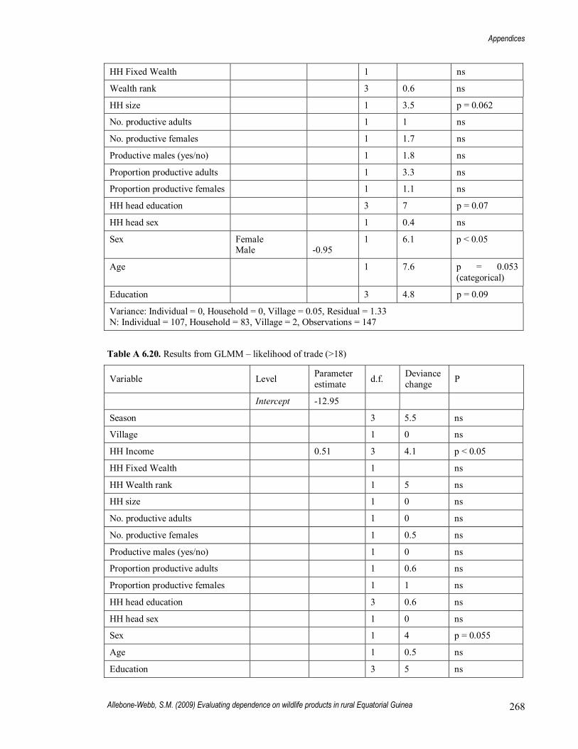
Appendices
Allebone-Webb, S.M. (2009) Evaluating dependence on wildlife products in rural Equatorial Guinea 268
HH Fixed Wealth 1 ns
Wealth rank 3 0.6 ns
HH size 1 3.5 p = 0.062
No. productive adults 1 1 ns
No. productive females 1 1.7 ns
Productive males (yes/no) 1 1.8 ns
Proportion productive adults 1 3.3 ns
Proportion productive females 1 1.1 ns
HH head education 3 7 p = 0.07
HH head sex 1 0.4 ns
Sex Female Male
-0.95
1 6.1 p < 0.05
Age 1 7.6 p = 0.053 (categorical)
Education 3 4.8 p = 0.09
Variance: Individual = 0, Household = 0, Village = 0.05, Residual = 1.33 N: Individual = 107, Household = 83, Village = 2, Observations = 147 Table A 6.20. Results from GLMM � likelihood of trade (>18)
Variable Level Parameter estimate d.f. Deviance
change P
Intercept -12.95
Season 3 5.5 ns
Village 1 0 ns
HH Income 0.51 3 4.1 p < 0.05
HH Fixed Wealth 1 ns
HH Wealth rank 1 5 ns
HH size 1 0 ns
No. productive adults 1 0 ns
No. productive females 1 0.5 ns
Productive males (yes/no) 1 0 ns
Proportion productive adults 1 0.6 ns
Proportion productive females 1 1 ns
HH head education 3 0.6 ns
HH head sex 1 0 ns
Sex 1 4 p = 0.055
Age 1 0.5 ns
Education 3 5 ns

Appendices
Allebone-Webb, S.M. (2009) Evaluating dependence on wildlife products in rural Equatorial Guinea 269
Variance : Individual = 2.7, HH = 0, Village = 0 n: Village = 2, HH = 152, Individual = 473, observations = 1348 Table A 6.21. Results from GLMM � amount of trade (>18)
Variable Level Parameter estimate d.f. Deviance
change P
Intercept 0.92
Season 1 Small Dry 2 First Wet 3 Big Dry 4 Second Wet
0.12 -0.73 -0.03
3 16 p < 0.01
Village 1 1 ns
HH Income 0.51 3 14 p < 0.001
HH Fixed Wealth 1 ns
HH Wealth rank 1 0.8 ns
HH size (sqrt) 1 1.4 ns
No. productive adults 1 0.5 ns
No. productive females 1 0.5 ns
Productive males (yes/no) 1 1 ns
Proportion productive adults 1 0.1 ns
Proportion productive females 1 0.1 ns
HH head education None Primary Secondary Higher
0.81 1.63 1.93
3 18 p < 0.001
HH head sex Female Male
-0.64
1 5 p < 0.05
Sex 1 0.5 ns
Age -0.24 1 5.3 p < 0.05
Education 3 3.7 ns
Variance : Individual = 0.55, HH = 0, Village = 0.038 n: Village = 2, HH = 58, Individual = 80, observations = 117

Appendices
Allebone-Webb, S.M. (2009) Evaluating dependence on wildlife products in rural Equatorial Guinea 270
Appendix 7. Accumulation strategies
Table A 7.1 Short term accumulation strategies. For 2005, respondents only ranked the severity of strategies that they had used. Frequency (freq.) refers to the number of households that report using this strategy in the previous 2 months. Average score refers to the average severity ranking (lower scores denoting the things that would be done first, with higher scores being the things that would be done only once the lower scoring things were also being done). The rank of scores is simply the average severity scores, ranked.
Freq. 2005 (both vill.s)
Av. Score 2005 (both vill.s)
Rank of av. Score (2005 both vill.)
Freq. Beayop 2005
Av. score Beayop 2005
Rank Beayop 2005
Freq. Teg 2005
Av. score Teg. 2005
Rank Teg. 2005
Save food for the next day
111 2 2 38 2 2 73 2 2
Eat 3 times or more each day
124 1 1 54 1.1 1 70 1 1
Sell food from agriculture or forest
113 2.8 3 44 2.55 3 69 2.96 3
Buy fish to eat 126 4.7 4 55 4.65 5 71 4.73 4
Buy meat to eat 122 5.05 5 51 4.61 4 71 5.37 6
Buy things for activities (cartridges, wire, hooks, machetes)
98 6.52 8 33 5.79 7 65 6.89 7
Buy preferred items (cigarettes, drinks, etc.)
81 7.07 9 27 6.48 8 54 7.37 8
Buy luxury items (clothes, jewerllery, shoes)
84 7.51 10 40 6.73 10 44 8.23 9
Help other members of the family
64 6.44 7 42 5.33 6 22 8.55 10
Pay off debts 70 5.29 6 19 6.53 9 51 4.82 5 Table A 7.2. Long term accumulation strategies. For 2005, respondents only ranked the severity of strategies that they had used. Frequency (freq.) refers to the number of households that report using this strategy in the previous 2 months. Average score refers to the average severity ranking (lower scores denoting the things that would be done first, with higher scores being the things that would be done only once the lower scoring things were also being done). The rank of scores is simply the average severity scores, ranked.
Strategy Freq. 2005 (both vill.s)
Av. Score 2005 (both vill.s)
Rank of av. Score (2005 both vill.)
Freq. Beayop 2005
Av. score Beay. 2005
Rank Beay. 2005
Freq. Teg 2005
Av. score Teg. 2005
Rank Teg. 2005

Appendices
Allebone-Webb, S.M. (2009) Evaluating dependence on wildlife products in rural Equatorial Guinea 271
Buy domestic animals 44 2.91 4 26 3.27 6 18 2.39 4
Buy regular equipment for activities (machetes, cestas, etc)
122 1.12 1 53 1.28 1 69 1 1
Buy large equipment for activities (guns, nets, etc)
15 2.4 3 7 2.71 3 8 2.13 2
Buy things for entertainment (radios, mobiles, etc.)
60 3.03 6 33 3.64 8 27 2.3 3
Buy material to construct the house (cement, chapas, nipas, tablas)
43 2.16 2 32 1.81 2 11 3.18 5
Buy things for the house (furniture, carpet, tv)
18 3.44 8 16 3.31 7 2 4.5 6
Buy big things for the house (grupo, bar, fridge)
12 3.25 7 12 3.25 5 0 NA NA
Buy a big thing (car, house) 1 3 5 1 3 4 0 NA NA
Put money in the bank 0 0 NA 0 NA NA 0 NA NA

Appendices
Allebone-Webb, S.M. (2009) Evaluating dependence on wildlife products in rural Equatorial Guinea 272
Appendix 8. Supplementary material: Chapter 5
Table A 8.1 Results from GLMM of household food security score from 2005 and 2006 against household level variables. The higher the food security score, the less food secure. Parameter estimates are shown for the minimum adequate model. Year and household nested within village were specified as random effects. The number of productive adults and females and proportion of productive adults and females were all correlated, so each parameter was fitted to the model in turn, and the parameter explaining the greatest deviance taken in the minimum adequate model.
Variable Level Parameter estimate
d.f. Deviance change
P
intercept 4.91
Village Beayop Teguete
2.38
1 6 p < 0.02
Income -0.016 1 64 p < 0.0001
Fixed Wealth -0.00063 1 14 p < 0.005
Wealth rank 1 2 3 4 5
-1.44 -1.48 -1.42 -1.95
1 10 p < 0.05
Proportion productive adults
-2.11 1 22 p < 0.0001
Variance: HH = 0, Village = 0.125, Year = 0.17, Residual variance = 5.76 n (Village) = 2, n (HH) = 143, n (year) = 2, n (observations) = 245
Table A 8.2. Results of LMM analysing the differences in the number of production sources/HH between villages and food security quartiles. Food security quartiles are taken as those from 2006 data and the least food secure quartile in each village compared to the rest of the population. Village specified as a random effect. The number of production sources was logged to give a normal distribution.
Variable Levels Parameter estimate
d.f. Deviance change
P
intercept 1.28
Village 1 3.5 ns
Food security Least secure (4) Rest (1-3)
-0.10 0
1 15.4 p < 0.001
Variance: Village = 1.83 e-10, Residual variance = 0.37 n: HH = 102

Appendices
Allebone-Webb, S.M. (2009) Evaluating dependence on wildlife products in rural Equatorial Guinea 273
Table A 8.3. Results of LMM analysing the differences in the number of income sources/HH between villages and food security quartiles. Food security quartiles are taken as those from 2006 data and the least food secure quartile in each village compared to the rest of the population. Village specified as a random effect. The number of income sources plus 1 was logged to give a normal distribution.
Variable Levels Parameter estimate
d.f. Deviance change
P
intercept 1.07
Village 1 -1.3 ns
Food security Least secure (4) Rest (1-3)
-0.23 0
1 22.2 p < 0.0001
Variance: Village = 0.0007, Residual variance = 0.25 n: HH = 102
Table A 8.4. Results of LMM analysing the differences in the number of production sources/HH between villages and wealth rank. The poorest wealth rank in each village was compared to the rest of the population. Village specified as a random effect. The number of production sources was logged to give a normal distribution.
Variable Levels Parameter estimate
d.f. Deviance change
P
intercept 0.84
Village 1 -2.2 ns
Wealth Rank Poorest (1) Rest (2-4)
0.50
1 10.2 p < 0.01
Village: WR 1 2.8 p = 0.096
Variance: Village = 1.69 e-10, Residual variance = 0.34 n: HH = 111
Table A 8.5. Results of LMM analysing the differences in the number of income sources/HH between villages and wealth rank. The poorest wealth rank in each village was compared to the rest of the population. Village specified as a random effect. The number of income sources plus one was logged to give a normal distribution.
Variable Levels Parameter estimate
d.f. Deviance change
P
intercept 0.64
Village 1 -2.6 ns
Wealth Rank Poorest (1) Rest (2-4)
0.43
1 10.6 p < 0.01
Variance: Village = 1.22 e-10, Residual variance = 0.24 n: HH = 111

Appendices
Allebone-Webb, S.M. (2009) Evaluating dependence on wildlife products in rural Equatorial Guinea 274
Table A 8.6 Results of GLMM testing the significance of household and season variables for the weight-age score for the under-fives. Weight to age was represented by the WAZ z-score, a score showing the standard deviation from the mean, normalised to account for difference deviations for each age and sex group. These data were taken from health centre records in Teguete from the years 1997-2000. Year and individual nested within household were all specified as random effects.
Variable Levels Parameter estimate
d.f. Deviance change
P
intercept -0.20
Season 1SmallDry 2FirstWet 3BigDry 4SecondWet
-0.07 0.16 0.08
1 8 p < 0.01
HH head education 3 6.6 (p = 0.08)
Age -0.08 1 5 p < 0.05
Sex Female Male
-0.66
1 8.7 p < 0.01
Variance: Person:HH = 0.98, HH = 0, Year = 0.0047, Residual variance = 0.27 n (HH) = 28, n(Person) = 52, n (year) = 6, n (observations) = 423, n (Season) = 4
Table A 8.7 Results of LMM for all WAZ scores, as taken from health centre records in Teguete, 1997-2000, and the results of my own data collection, 2005 and 2006. Individual, year and season were fitted as random effects. Year was fitted as a factor, not as a continuous variable.
Variable Levels Parameter estimate d.f. Deviance change P
intercept -0.57
Season 1 Small Dry 2 First Wet 3 Big Dry 4 Second Wet
-0.035 0.18 0.21
3 8 p < 0.05
Age -0.21 1 64 p < 0.0001
Year 1997 1998 1999 2000 2005 2006
0.17 0.30 0.26 0.37 0.93 0.27
6 26 p < 0.02
Variance: Individual = 0.92, Season = 0.0022, Year = 0.0039, Residual variance = 0.25 n (individual) = 243, n (season) = 4, n (observations) = 1185, n(Years) = 7
Table A 8.8. Results of compositional analysis on proportion value from different livelihood sources for village and food security quartiles. (FS 1-3 and 4) Food security quartiles are taken as those from 2006 data, and the difference in compositions assessed using a manova.
Forest Agriculture Paid Trade
Village F 15.05 3.91 0.62 1.81
d.f. 1 1 1 1

Appendices
Allebone-Webb, S.M. (2009) Evaluating dependence on wildlife products in rural Equatorial Guinea 275
p p < 0.001 p = 0.051 ns ns
FS quartile (06), gp
F 0.20 0.42 0.08 0.007
d.f. 1 1 1 1
p ns ns ns ns
residual sum of sq.s
(n (HH) = 101
8.18 10.68 5.54 4.28
Table A 8.9. Results of compositional analysis on proportion income from different livelihood sources for village and food security quartiles. (FS 1-3 and 4) Food security quartiles are taken as those from 2006 data, and the difference in compositions assessed using a manova.
d.f. Forest Agriculture Paid Trade
Village F 1 10.49 7.54 0.03 0.09
p p < 0.01 p < 0.01 ns ns
FS quartile (06), gp
F 1 0.40 0.03 0.75 0.16
p ns ns ns ns
residual sum of sq.s
89 7.82 14.47 4.47 10.23
Table A 8.10. Results of compositional analysis on proportion value from different livelihood sources for village and wealth ranks (1 and 2-4)
d.f. Forest Agriculture Paid Trade
Village F 1 12.62 2.70 1.52 0.54
p p < 0.001 ns ns ns
WR F 1 4.02 0.22 0.03 4.39
p p < 0.05 ns ns p < 0.05
WR : Village F 1 9.77 4.22 0.33 0.08
p p < 0.01 p < 0.05 ns ns
residual sum of sq.s
107 8.17 11.39 5.93 4.81
Table A 8.11. Results of compositional analysis on proportion income from different livelihood sources for village and wealth ranks (1 and 2-4)
d.f. Forest Agriculture Paid Trade
Village F 1 10.64 7.68 0.07 0.48
p p < 0.01 p < 0.01 ns ns
WR F 1 3.89 0.06 0.13 3.09
p p = 0.052 ns ns p = 0.08
residual sum of sq.s
96 8.57 15.98 7.91 10.67

Appendices
Allebone-Webb, S.M. (2009) Evaluating dependence on wildlife products in rural Equatorial Guinea 276
Table A 8.12. Results of compositional analysis on proportion value from different livelihood sources for village, food security (1-3 and 4) and seasons (1,3,4 and 2)
d.f. Forest Agriculture Paid Trade
Village F 1 122.95 0.79 6.08 7.45
p p < 0.0001 ns p < 0.05 p < 0.01
FS (1-3 and 4) F 1 3.50 0.01 2.81 0.49
p p = 0.062 ns p = 0.094 ns
Season (2 and 1,3,4)
F 1 0.30 0.82 0.81 0.10
p ns ns ns ns
residual sum of sq.s 444 50.94 73.3 28.94 23.82
Table A 8.13. Results of compositional analysis on proportion income from different livelihood sources for village, food security (1-3 and 4) and seasons (1,3,4 and 2)
d.f. Forest Agriculture Paid Trade
Village F 1 23.07 1.02 3.18 0.92
p p < 0.0001 ns p = 0.075 ns
FS (1-3 and 4) F 1 9.21 0.86 0.38 0.59
p p < 0.01 ns ns ns
Season (2 and 1,3,4)
F 1 0.47 4.31 0.31 1.41
p ns p < 0.05 ns ns
Village: FS F 1 12.64 7.35 0.12 0.25
p p < 0.001 p < 0.01 ns ns
residual sum of sq.s 283 28.39 55.29 41.50 47.46 Table A 8.14. Results of compositional analysis on proportion production from different livelihood sources for village, wealth rank (1 and 2-4) and seasons (1,3,4 and 2)
d.f. Forest Agriculture Paid Trade
Village F 1 21.84 0.30 9.33 5.93
p p < 0.0001 ns p < 0.01 p < 0.05
WR (1 and 2-4) F 1 8.90 0.07 2.27 9.72
p p < 0.01 ns ns p < 0.01
Season (2 and 1,3,4)
F 1 0.76 0.14 0.03 2.98
p ns ns ns p = 0.085
Village: FS F 1 16.15 4.18 1.21 0.96
p p < 0.0001 p < 0.05 ns ns
residual sum of sq.s 484 53.91 80.74 31.15 25.79

Appendices
Allebone-Webb, S.M. (2009) Evaluating dependence on wildlife products in rural Equatorial Guinea 277
Table A 8.15. Results of compositional analysis on proportion income from different livelihood sources for village, wealth rank (1 and 2-4) and seasons (1,3,4 and 2)
d.f. Forest Agriculture Paid Trade
Village F 1 21.85 0.45 4.86 1.01
p p < 0.0001 ns p < 0.05 ns
WR (1 and 2-4) F 1 9.14 0.60 0.29 8.02
p p < 0.01 ns ns p < 0.01
Season (2 and 1,3,4)
F 1 0.64 3.91 0.40 0.91
p ns p < 0.05 ns ns
residual sum of sq.s 308 33.54 61.98 44.25 50.15 Table A 8.16 Differences in food source composition between seasons and households.
Agriculture Bought Forest Gifts
p F p F p F p F
Village p < 0.005 9.4 p < 0.0001 75.9 p < 0.0001 146.6 ns 0.7
Season ns 0.2 ns 1.5 ns 1.0 ns 0.9
Food Security ns 1.0 ns 1.4 ns 0.4 ns 0.3
Village: Season
ns 0.6 ns 0.0006 ns 0.2 ns 0.9
Village: FS ns 0.8 ns 2.4 ns 1.8 p < 0.05 4.5
FS: Season ns 0.8 ns 0.001 ns 1.4 ns 0.5

Appendices
Allebone-Webb, S.M. (2009) Evaluating dependence on wildlife products in rural Equatorial Guinea 278
Appendix 9. Supplementary material, chapter 6
Table A 9.1. Correlations between explanatory variables for carcasses from Sendje. Numbers in bold are significant (p < 0.05) and are shown only for those values over 0.1.
Table A 9.2. Correlations between variables for carcasses from Midyobo.
Price/carcass Price/kg Mark-up Preference Method (target)
Mass 0.939 -0.229 0.365 0.255
Price/carcass 0.355 0.313
Price/kg 0.396 -0.21
Mark-up 0.168
Preference 0.139
Price/ carcass
Price/kg Mark-up Preference Proportion Fresh
Method (chance)
Mass (log) 0.983 -0.966 -0.246 -0.401 0.297 -0.413
Price/carcass (log) 0.950 0.206 0.492 -0.342 0.462
Price/kg -0.180 0.328 -0.335 0.405
Mark-up 0.140 -0.119 0.175
Preference -0.022 0.564

Appendices
Allebone-Webb, S.M. (2009) Evaluating dependence on wildlife products in rural Equatorial Guinea 279
Figure A 9.1. Graphs showing the interaction between season and capture method with likelihood of sale to market in Sendje.
3 BigDry 4 SecondWet 1 SmallDry 2 FirstWet
3 BigDry 4 SecondWet 1 SmallDry 2 FirstWet

Appendices
Allebone-Webb, S.M. (2009) Evaluating dependence on wildlife products in rural Equatorial Guinea 280
Figure A 9.2. Price per carcass against R max for bushmeat species sold in Bata market. Primates are shown in red.
Figure A 9.3. Average carcass Rmax and travel time for each catchment. Travel time is shown on a log scale.

Appendices
Allebone-Webb, S.M. (2009) Evaluating dependence on wildlife products in rural Equatorial Guinea 281
Figure A 9.4. Average km travelled for 2003 and 2005 for each species, Central market only. Species are listed in order of 2003 average km travelled.
0
10
20
30
40
50
60
Afric
a C
ivet
Liza
rdG
enet
Bird
Mar
sh C
ane
Rat
Gia
nt P
ango
linAf
rica
Palm
Civ
etSn
ake
Pang
olin
Cro
codi
leR
ed R
iver
Hog
Porc
upin
eM
andr
illG
ueno
nD
uike
r Red
Dui
ker B
lue
Sita
tung
a/Bu
shbu
ckTo
rtois
eG
iant
Pou
ched
Rat
Blac
k C
olob
us
Species
Ave
rage
km
trav
elle
d
(C
entr
al m
arke
t onl
y)
20032005
Figure A 9.5. Change in km travelled (2003 � 2005) for each species.

Appendices
Allebone-Webb, S.M. (2009) Evaluating dependence on wildlife products in rural Equatorial Guinea 282
Figure A 9.6. Average price of meat per kilo for the range of products or species within a food category in Central market, 2005. E.g. Each bushmeat species gives one data point within the category �bushmeat�. FDomesticMeat = Fresh domestic meat (predominantly beef and goat), Ffactory = frozen meat/fish sold from three warehouses, generally sold wholesale (usually in boxes of 10 or 20kg) but sold in units of 1 kilo in at least one warehouse), FrozenMarkSale = frzen meat/fish sold in the market, SmkdFishSold = Smoked fish sold in the market.

Appe
ndice
s
Alleb
one-
Web
b, S
.M. (
2009
) Eva
luatin
g de
pend
ence
on
wildl
ife p
rodu
cts in
rura
l Equ
ator
ial G
uinea
283
Tabl
e A
9.3
. Sho
win
g da
ta v
illag
e an
d m
arke
t car
cass
cou
nts,
and
othe
r spe
cies
attr
ibut
es.
Shad
ed c
ells
show
dat
a th
at w
ere
not i
nclu
ded
in th
e an
alys
es (s
how
n he
re fo
r ref
eren
ce).
See
follo
win
g pa
ge fo
r not
es.
Ani
mal
Sp
p na
mes
Se
ndje
V
illag
e
Send
je M
ark
et
Mid
yob
o Vill
age
Mid
yob
o M
arke
t 1
Mas
s (k
g) 2
Rm
ax
Pric
e/
carc
ass
Cen
tral
2003
3
(CFA
)
Pric
e/
carc
ass
Mun
doas
i 20
05 4
(CFA
)
Pric
e/
kg
dres
sed
20
03 5
(CFA
)
Pric
e/ k
g dr
esse
d 20
05 5
(CFA
)
Mar
k up
Send
je
2003
Pr
efer
ence
Sc
ore
6
Mar
k u
p M
idyo
bo
2005
Am
phib
ia
Gol
iath
frog
C
onra
ua g
olia
th
12
0 0
0 2.
1 N
A
NA
N
A
NA
N
A
NA
2.
76
NA
Bird
s B
irds
(see
tabl
e 2)
28
6 9
282
24
1.0
1.09
27
17
2653
43
70
4267
1.
917
3.67
2.
144
Spot
-nec
ked
otte
r 8 Ao
nyx
cong
ica
0 0
4 0
5.3
0.60
N
A
NA
N
A
NA
N
A
NA
N
A
Afr
ica
cive
t C
ivet
tictis
civ
etta
1
1 5
0 6
0.69
70
00
1400
0 17
95
3590
1.
917
4 N
A
Afr
ica
palm
civ
et
Nan
dini
a bi
nota
ta
26
17
38
28
2.4
0.66
62
09
8839
39
80
5666
1.
977
4 2.
212
Leop
ard
8 Pa
nthe
ra p
ardu
s 2
0 1
0 23
0.
36
NA
N
A
NA
N
A
NA
3.
09
NA
Gen
et &
Lin
sang
(s
ee ta
ble
2)
24
6 68
29
1.
7 0.
67
4000
33
00
3652
30
13
1.76
3.
53
1.97
3
Car
nivo
re
Mon
goos
e (s
ee ta
ble
2)
21
2 66
0
3.0
0.73
40
00
6000
20
51
3077
1.
833
2.33
N
A
Hyr
acoi
dea
Wes
tern
tree
hyr
ax
Den
droh
yrax
dor
salis
3
0 3
2 2.
8 0.
75
NA
30
00
NA
16
48
NA
N
A
NA
Mol
lusc
A
fric
an g
iant
sna
il Ac
hatin
a sp
p.
1 0
0 0
0.5
NA
N
A
NA
N
A
NA
N
A
3.31
N
A
Pang
olin
Ph
atag
inus
tric
uspi
s 32
4 12
1 58
0 20
4 2.
0 0.
70
4915
92
92
3781
71
48
1.79
7 4.
62
2.34
2 Ph
olio
dota
Gia
nt p
ango
lin
Smut
sia
giga
ntea
12
10
20
10
21
.0
0.37
5 63
250
7705
0 46
34
5645
1.
923
4.62
2.
449
Gue
nons
& m
anga
beys
9
(see
tabl
e 2)
26
9 22
1 56
1 55
3 4.
6 0.
11
7056
83
92
2244
28
06
2.01
7 4.
03
2.10
8
Bla
ck c
olob
us
Col
obus
sata
nus
378
134
449
449
9.5
0.20
70
37
8763
11
39
1419
1.
912
4.03
1.
914
Dem
idof
fs g
alag
o G
alag
oide
s dem
idof
f 0
0 1
0 0.
3 N
A
NA
N
A
NA
N
A
NA
4.
03
NA
Man
drill
M
andr
illus
sphi
nx
79
53
155
117
13.8
0.
18
3298
6 16
400
3677
18
28
2.17
7 4.
03
2.34
6
Nor
ther
n ta
lapo
in
Mio
pith
ecus
tala
poin
1
0 4
0 1.
2 0.
55
2955
15
00
3788
19
23
1.77
8 N
A
NA
Chi
mpa
nzee
n Pa
n tr
oglo
dyte
s 1
0 18
16
34
f 0.
07
NA
47
000
NA
21
27
2.43
8 1.
46
2.18
5
Prim
ate
Potto
(s
ee ta
ble
2)
3 1
4 0
1.0
f 0.
55
2500
N
A
3819
N
A
1.66
7 N
A
NA
Prob
osci
dea
Fore
st e
leph
ant 8
Loxo
dont
a af
rica
na
0 0
1 1
900
b 0.
10
NA
N
A
NA
N
A
NA
3.
76
NA
Afr
ica
fore
st tu
rtle
Kiny
xis e
rosa
86
5 26
1 66
5 62
0 1.
7 0.
89
3048
38
29
2758
34
66
2.00
2 3.
40
2.99
3 R
eptil
e
Dw
arf c
roco
dile
O
steo
laem
us te
tras
pis
135
127
56
40
6 0.
57
2305
7 32
281
5912
82
77
1.71
6 4.
41
2.23
5

Appe
ndice
s
Alleb
one-
Web
b, S
.M. (
2009
) Eva
luatin
g de
pend
ence
on
wildl
ife p
rodu
cts in
rura
l Equ
ator
ial G
uinea
28
4
Mon
itor l
izar
d Va
ranu
s nilo
ticus
21
13
14
8
4.2
0.65
70
93
1383
3 25
98
5067
1.
890
2.15
2.
573
Snak
e (s
ee ta
ble
2)
0 0
4 0
23.6
0.
38
NA
13
600
NA
88
7 N
A
1.85
2.
296 z
Bru
sh-ta
il po
rcup
ine
Athe
ruru
s afr
ican
us
2207
44
1 14
67
784
3.2
0.60
74
92
1119
5 36
02
5382
2.
001
4.65
2.
282
Gia
nt p
ouch
ed ra
t C
rice
tom
ys e
min
i 38
2 11
47
2 42
1.
1 0.
70
2692
27
41
3765
38
33
1.68
5 3.
75
2.69
4
Mar
sh c
ane
rat
Thry
onom
ys sw
inde
rian
us14
4
51
4 4.
7 0.
62
1036
4 12
786
3392
41
85
2.02
1 4.
17
2.6
Rod
ent
Squi
rrel
(s
ee ta
ble
2)
2 0
17
0 0.
3 1.
65
NA
N
A
NA
N
A
NA
2.
65
NA
Blu
e du
iker
C
epha
loph
us m
ontic
ola
2399
61
5 20
75
898
4.8
0.49
70
40
6998
22
56
2243
1.
995
4.14
2.
097
Red
dui
ker (
med
ium
) (s
ee ta
ble
2)
201
142
311
224
17.8
0.
20
3519
6 25
631
3038
22
12
2.00
7 3.
78
2.54
5
Red
dui
ker (
larg
e)
(see
tabl
e 2)
15
11
6
2 33
.9
0.30
53
127
5775
0 24
15
2625
1.
856
3.78
2.
2
Wat
er c
hevr
otai
n H
yem
osch
us a
quat
icus
10
2
27
4 9
0.50
16
500
15
500
2821
26
50
2.01
4 N
A
2.26
1
Dw
arf a
ntel
ope
Neo
trag
us b
ates
i 3
0 19
0
2.9
0.74
25
00
4167
13
26
2210
1.
694
4.14
N
A
Red
Riv
er H
og
Pota
moc
hoer
us p
orcu
s 15
14
30
7
30.5
0.
45
7145
0 69
895
3604
35
26
1.93
2 4.
57
2.82
Ung
ulat
e
Buf
falo
8 Sy
ncer
os c
affe
r 0
1 0
0 28
5 b
NA
N
A
NA
N
A
NA
N
A
3.65
N
A
1 Th
is is
an e
stim
ate
from
the
sam
ple
(dat
a w
as c
olle
cted
on
alte
rnat
e da
ys).
Onl
y da
ta r
ecor
ded
as c
omin
g fr
om M
idyo
bo (
rath
er th
an M
idyo
bo a
nd
Tegu
ete)
was
incl
uded
, pro
babl
y le
adin
g to
an
unde
r-es
timat
ion
of q
uant
ities
. 2 Ta
ken
from
Kum
pel (
2006
) unl
ess o
ther
wis
e sp
ecifi
ed. T
he w
eigh
ted
mas
s is u
sed
for g
roup
s of s
peci
es.
3 Fr
om K
umpe
l (20
06).
Pric
es a
re fo
r adu
lt fr
esh
carc
asse
s onl
y (r
athe
r tha
n al
l adu
lt ca
rcas
ses)
, so
som
e va
riatio
n fr
om h
er th
esis.
4 A
vera
ge a
dult
carc
ass p
rice
for B
ata
mar
kets
, 200
5.
5 Pr
ice
per d
ress
ed k
ilo c
alcu
late
d us
ing
pric
e pe
r car
cass
of f
resh
adu
lt ca
rcas
ses
only
. Dre
ssed
wei
ght c
alcu
late
d as
65%
of a
vera
ge fr
esh
adul
t car
cass
w
eigh
t.
6 Pr
efer
ence
scor
e fr
om N
ick�
s m
aste
rs (a
nd b
ook
chap
ter �
che
ck if
/whe
n pu
blis
hed)
. Res
pond
ents
ask
ed to
giv
e a
scor
e ou
t of 5
for a
rang
e of
food
s (1
= ha
te, 5
= lo
ve).
Ave
rage
scor
e is
show
n. N
= 4
1.
8 Ex
clud
ed fr
om a
naly
ses
due
to la
ck o
f pric
e da
ta.
9 G
ueno
ns a
nd m
anga
beys
wer
e co
mbi
ned
due
to a
hig
h fr
eque
ncy
of m
isid
entif
icat
ion
(par
ticul
arly
of s
mok
ed c
arca
sses
). N
o m
anga
beys
wer
e re
cord
ed
in 2
005
b Fr
om (K
ingd
on 1
997)
. g A
vera
ge p
rice
for g
roup
, wei
ghte
d by
pro
porti
on o
f diff
eren
t spe
cies
. i A
lthou
gh th
ere
wer
e so
me
man
drill
s bo
ught
for
equ
al to
, or
grea
ter
than
the
2003
pric
e, th
ere
wer
e al
so a
larg
e nu
mbe
r of
low
val
ue m
andr
ills.
Even
w
hen
the
pric
e of
onl
y fr
esh
or a
live
adul
ts w
as t
aken
(i.e
. ex
clud
ing
low
er v
alue
sm
oked
and
rot
ten
carc
asse
s),
the
aver
age
was
onl
y 23
,770
cfa
. Si
mila
rly, a
lthou
gh s
ome
red
duik
ers
are
mor
e ex
pens
ive
that
the
2003
pric
es. F
resh
adu
lt av
erag
e is
27,7
18 c
fa. S
ome
of th
e 20
05 p
rices
are
low
er th
an
the
2003
pric
es. T
his i
s mai
nly
beca
use
the
pric
es in
mun
daos
i mar
ket w
ere
gene
rally
low
er th
an th
ose
in c
entra
l mar
ket.
z Sn
ake
has
a m
ark-
up v
alue
for m
idyo
bo (d
espi
te 0
reco
rded
in m
arke
t) be
caus
e on
e w
as re
cord
ed in
the
mar
ket,
but i
n th
e co
ld w
et s
easo
n (w
hen
none
re
cord
ed in
vill
age)
.

Appendices
Allebone-Webb, S.M. (2009) Evaluating dependence on wildlife products in rural Equatorial Guinea 285
Table A 9.4. Species composition of groups referred to in Table A 9.3.

Chapter 1: Introduction
286
Birds
Black guinea fowl
Black-casqued wattled hornbill
Black-and-white casqued hornbill
Great blue turaco
Scaly francolin
Guinea fowl unknown
Plumed guinea fowl
Palm-nut vulture
Nkulengu rail
Pigeon/DoveSpp
Africa grey parrot
Hartlaub's duck
Crowned hawk-eagle
Agelastes niger
Ceratogymna atrata
Ceratogymna subcylindricus
Corythaeola cristata
Francolinus squamatus
Guinea fowl unknown
Guttera plumifera
Gypohierax angolensis
Himatornis haematopus
Pigeon/DoveSpp
Psittacus erithacus
Pteronetta hartlaubi
Stephanoaetus coronatus
Genets
Servaline genet
Central african linsang
Genetta servalina
Poiana richardsoni
Mongooses
Marsh mongoose
Black-legged mongoose
Cuisimanse
Mongoose unknown
Long-snouted mongoose
Atilax paludinosus
Bdeogale nigripes
Crossarchus platycephalus
NA
Herpestes naso (None in Sendje)
Mangabey Grey-cheeked mangabey Lophosebus albigena
Great apes
Western lowland gorilla
Chimpanzee
Gorilla gorilla gorilla
Pan troglodytes
Pottos
Potto
Golden angwantibo
Perodicticus potto
Artocebus aureus
Snakes
Gabon viper
African rock python
Bitis gabonica
Python sebae
Squirrel
Biafran bight palm
Rope squirrels
Red-legged sun squirrel
African pygmy squirrel
African giant squirrel
Epixerus wilsoni
Funisciurus spp
Heliosciurus rufobrachium
Myosciurus pumilio
Protoxerus strangeri
Red duikers (medium)
Peter's duiker
Ogilby's duiker
Bay duiker
White-bellied duiker
Black-fronted duiker
Yellow-backed duiker
Cephalophus callypigus
Cephalophus ogilbyi
Cephalophus dorsalis
Cephalophus leucogaster
Cephalophus nigrifrons
Cephalophus silvicultor
Gorilla Seen once in the wild near Midyobo, and possibly recorded in the market, but
unconfirmed.
Red duikers (large) Bush buck
Sitatunga
Tragelaphus scriptus
Tragelaphus spekei

Chapter 1: Introduction
287

Chapter 1: Introduction
288
Appendix 10. Product Lists: consumption and prices
Table A 10.1 Common agricultural food items
Shows the proportion of interviews where each agricultural food item was recorded as consumed (i.e. the proportion of sample days per household) for the most common agricultural foods, and the average price per unit for each village. Items are shown in order (most frequently consumed first).
Proportion of interviews where consumption
recorded
Average price per unit (cfa) Food item
Beayop Teguete
Most Common
Unit Beayop Teguete
Cassava (bar) 0.71 0.81 Bar 55 50 Chilli Pepper 0.59 0.53 Pile 25 50 Leaves (all types) * 0.58 0.46 Packet 170 147 Onion 0.83 0.39 Entire 94.1 83.6 Palm Oil * 0.29 0.36 Litre 500 500 Cassava (boiled) 0.28 0.28 Basin 150 150 Banana 0.04 0.27 Entire 19.5 16.7 Peanut 0.47 0.25 Sack50 11203 13461 Cassava leaves 0.28 0.18 Packet 100 100 Pineapple <0.01 0.14 Entire 95 Calabaza 0.04 0.11 Sack50 20000 18661 Avocado 0.04 0.05 Entire 50 25 Maize 0.14 0.03 Basin 117 116 Plantain 0.26 0.03 Stalk 1527 1500 Tomatoes (fresh) 0.35 0.03 Plate 100 50 Cocoyam 0.06 0.02 Entire 25 Yam 0.01 0.02 Entire 50 50 Orange <0.01 0.02 Entire 31 Papaya 0.01 0.01 Entire 325 200 Sugar Cane <0.01 <0.01 Sack50 2000 3000 Goat (fresh) <0.01 <0.01 Entire 10000 Guinean potatoes <0.01 <0.01 Entire 33 50 Eggs <0.01 <0.01 Entire 100 Sugared peanuts <0.01 <0.01 Piece 50 Banana bunuelo <0.01 <0.01 Entire 7.1 Bread fruit <0.01 <0.01 Entire 25 Herbs <0.01 <0.01 Entire 16.6 25 Sugar cane wine Litre 243 138
All agricultural products 0.998 0.997

Chapter 1: Introduction
289
Table A 10.2 Common coastal food items
Shows the proportion of interviews where this item was recorded as consumed, and the average price per unit for each village, for the most frequently consumed items. Local names for fish species are given. The total includes rare and unspecified fish. Items are shown in order (most frequently consumed first).
Proportion of interviews where consumption
recorded
Average price per unit (cfa) Food item
Beayop Teguete
Most common
Unit Beayop Teguete
�Bifaka� (smoked) 0.29 0.12 Entire 62.9 43.4 �Celele� (smoked) <0.01 0.15 Pile 101.4 �Abamikono� (smoked) 0.01 <0.01 Entire 550 �Biconot� (smoked) 0.01 <0.01 Entire 71.43 �Meneng� (smoked) <0.01 <0.01 Entire 150
All coastal products 0.33 0.27
Table A 10.3 Imported food items
Shows the proportion of interviews where this item was recorded as consumed and the average price per unit for each village, for the most frequently consumed imported items. The proportion of sampe days consumed is not shown for alcoholic drinks, as these numbers are likely to be an underestimate. Items are in order.
Proportion of interviews where consumption
recorded
Average price per unit (cfa) Food item
Beayop Teguete
Most Common
Unit Beayop Teguete
Salt 0.94 0.85 Glass 100 100 Stock cubes (maggi) 0.89 0.72 Caldo 50.1 47.7 Rice 0.32 0.11 Glass 100 100 Vegetable Oil 0.32 0.09 Litre 980 1000 Mackerel (frozen) 0.32 0.08 Kg 795.1 785 Tomatoes (tinned) 0.13 0.07 Tin 101 144 Chicken (frozen) 0.12 0.05 Kg 1250 1275 Bunuelos (flour) 0.08 0.09 Entire 25.2 36.6 Sugar 0.03 0.03 Cube 6.3 5.6 Sardines (tinned) 0.03 0.02 Tin 302 324 Pig (frozen) 0.03 <0.01 Kg 1281.8 Beef (frozen) 0.01 <0.01 Kg 1300 Spagetti 0.01 <0.01 Packet 425 400 Turkey (frozen) <0.01 <0.01 Kg 1300 Spam <0.01 <0.01 Tin 800 Bonito (frozen fish) <0.01 <0.01 Kg 800 Caramelos <0.01 <0.01 Entire 30 23.8 Leche en lata <0.01 <0.01 Tin 600 625 Vino Litre 686 780 Cerveza Can 700 700 Conac Small glass 100 125
All frozen fish 0.346 0.083
All frozen domestic meat 0.171 0.051
All imports 0.975 0.905

Chapter 1: Introduction
290
Table A 10.4 Wild food items
Proportion Interviews where consumption recorded
Average price per unit (cfa) Food item
Beayop Teguete
Most Common Unit
Beayop Teguete
Wild Animals Blue duiker 0.043 0.095 Entire 3657 2696 Giant pouched rat 0.027 0.062 Entire 1421 913 Bay duiker 0.005 0.057 Entire 10250 6735 Moustached monkey 0.005 0.048 Entire 3571 2694 Brush-tailed porcupine 0.004 0.045 Entire 5250 3751 Black colobus <0.001 0.024 Entire 4094 Marsh cane rat 0.007 0.010 Entire 3778 3500 Pangolin 0.005 0.011 Entire 3132 1835 Putty-nosed monkey 0.002 0.013 Entire 3103 Snail 0.005 <0.001 Entire 50 Mandrill <0.001 0.005 Entire 11464 Sitatunga 0.004 <0.001 Entire 10000 Snake 0.004 <0.001 Entire 4400 Wild bird 0.005 0.003 Entire 800 625 Lizard 0.002 0.003 Entire 3625 3083 Genet 0.002 <0.001 Entire 2500 African civet 0.002 <0.001 Entire 7000 Dwarf antelop 0.002 <0.001 Entire 2177 African palm civet 0.002 0.002 Entire 3167 2333 Cuisimanse 0.002 0.002 Entire 1000 2500 Tortoise 0.002 0.002 Entire 1938 1007 Red river hog <0.001 0.002 Entire 35000 Squirrel <0.001 <0.001 Entire 950 500 Chimpanzee <0.001 <0.001 Entire 15667 Crocodile <0.001 <0.001 Entire 1000 Nkwa - jirafa <0.001 <0.001 Entire 13000 16000 Onzem - titi <0.001 <0.001 Entire 1500 Giant Pangolin <0.001 <0.001 Entire 25000
All wild animals 0.122 0.359
Wild Fish
Fresh water crabs 0.020 0.043 Entire 100 �Ndo� 0.052 0.002 Entire 128 �Mifiga� 0.020 <0.001 Entire 196 �Mikeme� 0.009 <0.001 Entire 286 286 �Bifaka� (fresh) 0.005 Entire 27.3 �Awom� <0.001 Entire 49 �Ndjobo� <0.001 Entire 250 �Ndo� <0.001 <0.001 Entire 67 100 �Ngo� (fresh) <0.001 <0.001 Entire 334 333 �Ngo� (smoked) <0.001 Entire 500 �Nkara� <0.001 Entire 27.3

Chapter 1: Introduction
291
�Nkó� <0.001 Entire 100 �Nva�� <0.001 Entire 62.5 All wild fish 0.165 0.143
Wild Plants
Chocolate 0.120 0.480 Escudilla 4125 3600 African Plum 0.013 0.059 Entire 35 7.5 Palm wine Litre 200 107 Forest Fruits (all species) 0.037 Plate 50 All wild plants 0.14 0.52
Table A 10.5 Average prices of non-food items, Beayop and Teguete
English Name Most Common Unit Average Price Beayop (cfa) Average Price Teguete (cfa)
Wire Metre 200 350
Fishing Hook Entire 25 25
Gun cartridge Entire 600 650
File Entire 900 1000
Machete Entire 2400 2500
Cigarette Packet 494.7 496.5
Soap Entire 171.9 138.6
Gasoline Litre 350 353
Wicker basket Entire 1750 1500
Fish trap Entire 2000
Wicker dish Entire 317 300
Raffia Entire 200