euler systems (arizona winter school 2018 notes)...
TRANSCRIPT

Euler systems (Arizona Winter School 2018 notes)
David Loeffler and Sarah Livia Zerbes


Introduction
The theory of Euler systems is one of the most powerful tools available for studyingthe arithmetic of global Galois representations. However, constructing Euler sys-tems is a difficult problem, and the list of known constructions was until recentlyaccordingly rather short. In these lecture notes, we outline a general strategy forconstructing new Euler systems in the cohomology of Shimura varieties: these Eulersystems arise via pushforward of certain units on subvarieties.
We study in detail two special cases of this construction: the Euler system ofBeilinson–Flach elements, where the underlying Shimura variety is the fibre productof two modular curves; and the Euler system of Lemma–Flach elements, arising inthe cohomology of Siegel modular threefolds.
The lecture notes are structured as follows.
• In Chapter 1, we will review the definition of Euler systems for Galoisrepresentations, and their arithmetic application to the Bloch–Kato con-jecture.
• In Chapter 2, we introduce some general tools for constructing global co-homology classes for Galois representations arising in geometry, assumingthe existence of a supply of subvarieties of appropriate codimension andunits on them. We also introduce Siegel units, which are the key for allthe Euler system constructions to follow.
• Chapter 3 is largely motivational (and can be skipped at a first reading):it explains how one can use Rankin–Selberg-type integral formulas forL-functions as a guide to where to look for Euler systems.
• Chapter 4 is devoted to the construction of the Beilinson–Flach Eulersystem for pairs of modular forms of weight 2; and in Chapter 5, wediscuss how to adapt this construction to pairs of modular forms of higherweight, using cohomology with coefficients.
• In Chapter 6 we explain the construction of the Lemma–Flach Euler sys-tem for genus 2 Siegel modular forms of parallel weight 3.
• In the concluding Chapter 7 we outline some projects.
Updated 13/2/2018, incorporating corrections from Chi-Yun Hsu.
3


Contents
Introduction 3
Chapter 1. Galois representations and Galois cohomology 71.1. Galois representations 71.1a. Definitions 71.1b. Examples 71.1c. Representations coming from geometry 81.2. L-functions of Galois representations 81.2a. Local Euler factors 81.2b. Global L-functions (sketch) 81.3. Galois cohomology 91.3a. Setup 91.3b. The Kummer map 91.3c. Selmer groups 101.3d. The Bloch–Kato conjecture 111.4. Euler systems 121.4a. The definition 121.4b. Cyclotomic units 141.4c. Soule twists 14
Chapter 2. A toolkit for building Euler systems 172.1. Etale cohomology and the Hochschild–Serre spectral sequence 172.2. Modular curves and modular forms 182.2a. Modular curves 182.2b. Galois representations 192.2c. Tensor products 192.3. Numerology 202.4. Changing the field and changing the level 212.5. Siegel units 222.5a. The construction 222.5b. Changing the level: the basic norm relation 23
Chapter 3. Interlude: motivic cohomology and period integrals 253.1. The Rankin–Selberg integral formula 253.2. Motivic cohomology 263.3. Other Rankin–Selberg formulae 273.4. P-adic regulators 28
Chapter 4. The Beilinson–Flach Euler system 314.1. Beilinson–Flach elements 31
5

6 CONTENTS
4.1a. Strategy 314.1b. Mixed-level modular curves 324.1c. Rankin–Eisenstein classes 334.1d. Beilinson–Flach elements 334.2. Norm-compatibility 334.3. Projection to the (f, g) component 36
Chapter 5. Modular forms of higher weight 395.1. Galois representations 395.2. Eisenstein classes 405.3. The Euler system for higher weight modular forms 405.3a. Pushforward with coefficients 405.3b. Definition of the classes 415.4. Twist-compatibility 425.5. An adelic modification 42
Chapter 6. An Euler system for Siegel modular forms 456.1. Siegel modular 3-folds 456.2. Genus 2 Siegel modular forms 466.2a. Definitions 466.2b. Hecke operators 466.3. Galois representations 476.4. Lemma-Flach elements 486.4a. Strategy 486.4b. Motivation: integral formulae 496.4c. Lemma–Eisenstein classes 496.4d. Norm relations 506.4e. Lemma-Flach classes and their norm relations 51
Chapter 7. Projects 537.1. An Euler system for GSp4×GL2 537.2. Euler systems and Selmer groups in Coleman families 54
Bibliography 55

CHAPTER 1
Galois representations and Galois cohomology
References: for §§1.1—1.3, an excellent source is Bellaiche’s CMI notes on theBloch–Kato conjecture.
1.1. Galois representations
1.1a. Definitions. Let K be a number field, K its algebraic closure, GK =Gal(K/K); and let p be a prime, and E a finite extension of Qp. We’re interestedin representations of GK on finite-dimensional E-vector spaces V .
We always assume that
(1) ρ : GK → Aut(V ) ∼= GLd(E) is continuous (where d = dim(V )), withrespect to profinite topology of GK and the p-adic topology on GLd(E).
(2) V is “unramified almost everywhere”: for all but finitely many primeideals v of K, we have ρ(Iv) = {1}, where Iv is an1 inertia group at v.
1.1b. Examples.
The representation Zp(1). Let µpn = {x ∈ K× : xpn
= 1}. Then µpn is finitecyclic of order pn and GK acts on it.
The p-power map sends µpn+1 → µpn and we define
Zp(1) := lim←−n
µpn , Qp(1) := Zp(1)⊗Qp.
This is a 1-dimensional continuous Qp-linear representation, unramified outside theprimes dividing p; GK acts by “cyclotomic character” χcyc : GK → Z×p .
(Notation: for any V , n ∈ Z, we set V (n) = V ⊗Qp(1)⊗n.)
Tate modules of elliptic curves. A/K elliptic curve⇒ A(K) abelian group withGK-action. Let A(K)[pn] subgroup of pn-torsion points.
Define
Tp(A) := lim←−n
A(K)[pn] (w.r.t. multiplication-by-p maps), Vp(A) := Tp(A)⊗Qp.
This is a 2-dimensional continuous GK-representation, unramified outside the set{v : v | p} ∪ {v : A has bad reduction at v}. (The same works for abelian varietiesof any dimension g, giving 2g-dimensional representations of GK .)
1Iv depends on a choice of prime of K above v, but only up to conjugation in GK , so whetheror not V is unramified at v is well-defined.
7

8 1. GALOIS REPRESENTATIONS AND GALOIS COHOMOLOGY
Etale cohomology. Let X/K be a smooth algebraic variety. We can definevector spaces
Hiet(XK ,Qp) for 0 ≤ i ≤ 2 dimX,
which are finite-dimensional p-adic Galois representations, unramified outside p andprimes of bad reduction2 of X.
1.1c. Representations coming from geometry. Our second example isa special case of the third: for an elliptic curve A, it turns out that we haveVp(A) ∼= H1
et(AK ,Qp)(1).
Definition. We say an E-linear Galois rep V comes from geometry if it is asubquotient of Hi
et(XK ,Qp)(j) ⊗QpE, for some variety X/K and some integers
i, j.
So all my examples come from geometry. In these lectures we’re only ever going tobe interested in representations coming from geometry.
Remark. Conjecturally the representations coming from geometry should be ex-actly those which are continuous, unramified almost everywhere, and potentiallysemistable at the primes above p (a technical condition from p-adic Hodge theory).This is called the Fontaine–Mazur conjecture. �
1.2. L-functions of Galois representations
1.2a. Local Euler factors. Let V as above, v unramified prime. Thenρ(Frobv) is well-defined up to conjugacy, where Frobv is the arithmetic Frobenius.
Definition. The local Euler factor of V at v is the polynomial
Pv(V, t) := det(1− t · ρ(Frob−1v )) ∈ E[t].
Examples:
V Pv(V, t)Qp 1− t
Qp(n) 1− tqnv, qv = #Fv
H1(AK ,Qp) 1− av(A)t+ qvt2, av(A) := 1 + qv −#A(Fv)
1.2b. Global L-functions (sketch). Assume V comes from geometry, andV is semisimple (direct sum of irreducibles). Then Pv(V, t) has coefficients in Q(Deligne); and there is a way of defining Pv(V, t) for bad primes v (case v | p ishardest).
Fix an embedding ι : Q ↪→ C. Then we consider the product
L(V, s) :=∏
v prime
Pv(V, q−sv )−1.
Miraculously, this converges for <(s)� 0.
2This is a little delicate to define properly if we don’t assume X to be proper over K.Formally, we say X has “good reduction” at v if it’s isomorphic to the complement of a relative
normal crossing divisor in a smooth proper OK,v-scheme.

1.3. GALOIS COHOMOLOGY 9
E.g. for V = Qp(n) this is ζK(s+n), where ζK is the Dedekind zeta function of K(which is just the Riemann zeta for K = Q). For V = H1(AK ,Qp), A an ellipticcurve, it is the Hasse–Weil L-function L(A/K, s).
Conjecture 1. For V semisimple and coming from geometry, L(V, s) has mero-morphic continuation to s ∈ C with finitely many poles, and satisfies a functionalequation relating L(V, s) and L(V ∗, 1− s).
Note that if V is semisimple and comes from geometry, the same is true3 of V ∗,so the conjecture is well-posed. This conjecture is of course super-super-hard – theonly cases where it is known is where we can relate V to something automorphic,e.g. a modular form.
There are lots of conjectures (and a rather smaller set of theorems) relating proper-ties of arithmetic objects to values of their L-functions; the Birch–Swinnerton-Dyerconjecture is perhaps the best-known of these. As we’ve just seen, all the infor-mation about an elliptic curve you need to define its L-function is encoded in theGalois action on its Tate module; so can we express the BSD conjecture purely interms of Galois representations? This will be the topic of the next section.4
1.3. Galois cohomology
1.3a. Setup. There is a cohomology theory for Galois representations5: forV an E-linear GK-rep, we get E-vector spaces Hi(K,V ), zero unless i = 0, 1, 2.Mostly we care about H0 and H1, which are given as follows
H0(K,V ) = V GK
H1(K,V ) ={cts fcns s : GK → V such that s(gh) = s(g) + gs(h)}{fcns of the form s(g) = gv − v for some v ∈ V }
.
These are well-behaved: short exact sequences of V ’s give long exact sequences ofcohomology, for instance. Unfortunately they’re not finite-dimensional in general.
1.3b. The Kummer map. For V = Qp(1) the Galois cohomology is relatedto the multiplicative group K∗. To see this, we have to first think a bit aboutcohomology with finite coefficients.
For any n, we have a short exact sequence
0 - µpn - K× [pn]- K
× - 0
which leads to a long exact sequence
0 - µGKpn - K×[pn]- K× - H1(K,µpn)
3It is not obvious if this holds without the semisimplicity assumption.4Actually the answer is “no, we can’t” – as far as I’m aware, there is no purely Galois-
representation-theoretic statement that is precisely equivalent to BSD. But we can get prettyclose, as we’ll shortly see.
5Technical point: our representations are all continuous, so we shall work with cohomologydefined by continuous cochains, which is slightly different from the cohomology of GK as an
abstract group.

10 1. GALOIS REPRESENTATIONS AND GALOIS COHOMOLOGY
and thus an injection6
K× ⊗ Z/pnZ ⊂ - H1(K,µpn).
Passing to the inverse limit we get a map (Kummer map)
κp : K× ⊗ Zp ⊂ - H1(K,Zp(1)) or K× ⊗Qp⊂ - H1(K,Qp(1)).
Remark. This already shows that H1(K,Qp(1)) can’t be finite-dimensional, be-cause K× has countably infinite rank. �
The same argument works for elliptic curves: we get an embedding
E(K)⊗Qp⊂ - H1(K,Vp(E)).
1.3c. Selmer groups. Since the groupsH1(K,V ) can be infinite-dimensional,it’s useful to “cut down to size” by imposing extra conditions on our H1 elements.We’ll do this by localising at primes of K. Note that we have maps
Hi(K,V )→ Hi(Kv, V ) for all primes v,
and the local groups Hi(Kv, V ) are finite-dimensional.
Definition. A local condition on V at prime v is an E-linear subspace Fv ⊆H1(Kv, V ).
Examples:
• strict local condition Fv,strict = {0}• relaxed local condition Fv,relaxed = everything• unramified local condition
Fv,ur = image(H1(GKv/Iv, V
Iv )→ H1(Kv, V ))
• Bloch–Kato “finite” local condition Fv,BK (for v | p) – defined using p-adicHodge theory.
Definition. A Selmer structure is a collection F = (Fv)v prime of K , satisfying thefollowing condition: for almost all v we have Fv = Fv,ur. If F is a Selmer structurewe define the corresponding Selmer group by
SelF (K,V ) = {x ∈ H1(K,V ) : locv(x) ∈ Fv ∀v}.
Theorem 1 (Tate). For any Selmer structure F , the space SelF (K,V ) is finite-dimensional over Qp.
Sketch of proof. It’s easy to see that if this statement is true for one F , it’strue for any F , since the local Galois cohomology groups H1(Kv, V ) are all finite-dimensional. We now choose a particular Selmer structure F (exercise: which?)such that SelF (K,V ) is the image of the map
H1(Gal(KΣ/K), V
)↪→ H1(K,V ),
where KΣ is the maximal extension of K unramified outside some finite set of placesΣ containing all infinite places, all places above p, and all places where V is ramified.This reduces us to what Tate actually proved, which is that the cohomology groupsof Gal
(KΣ/K
)are finite-dimensional. �
6In fact this is an isomorphism, because H1(K,K×
) is zero (“Hilbert’s theorem 90”)

1.3. GALOIS COHOMOLOGY 11
We’re mostly interested in three specific choices of Selmer structure, differing only inthe choices of the Fv at primes v | p: we define the strict Selmer group Selstrict(K,V )by taking Fv = Fv,ur for v - p, and Fv = Fv,strict for v | p; and similarly the relaxedSelmer group and Bloch–Kato Selmer group.
Hence the strict, relaxed, and Bloch–Kato Selmer groups satisfy
Selstrict(K,V ) ⊆ SelBK(K,V ) ⊆ Selrelaxed(K,V ).
Remark. As will soon become clear, it is SelBK(K,V ) which is the most importantof all. We care about Selstrict(K,V ) and Selrelaxed(K,V ) because they are easier tostudy, and will give us a stepping-stone towards SelBK(K,V ). �
Example. Recall that for V = Qp(1) we had the Kummer map
K× ⊗Qp⊂ - H1(K,Qp(1)).
One can check that this induces isomorphisms
OK [1/p]× ⊗Qp
∼=- Selrelaxed(K,Qp(1)),
O×K ⊗Qp
∼=- SelBK(K,Qp(1)).
The strict Selmer group, on the other hand, should be zero; this is exactly Leopoldt’sconjecture for K. �
1.3d. The Bloch–Kato conjecture. Let V be a representation coming fromgeometry.
Conjecture 2 (Bloch–Kato). We have
dim SelBK(K,V )− dimH0(K,V ) = ords=0 L(V ∗(1), s).
There are refined versions using Zp-modules in place of Qp-vector spaces, whichpredict the leading term of the L-function up to a unit; but we won’t go into thesehere.
Let’s look at what the conjecture says in some example cases.
Example 1: V = Qp. Here L(V ∗(1), s) = L(Qp, s + 1) = ζK(s + 1), so theright-hand side is the order of vanishing of ζK(s) at s = 1, which is −1 for every K(there’s a simple pole). The left-hand side is dim SelBK(K,Qp)−1, so the conjecturepredicts that SelBK(K,Qp) = 0.
Exercise: Prove this. You’ll need to use the finiteness of the ideal class group of K,together with the fact that for this representation the local condition Fv,BK agreeswith Fv,ur for primes v | p.
Example 2: V = Qp(1). Here L(V ∗(1), s) = ζK(s). Inspecting the functionalequation for Dedekind zeta functions, we see that ords=0 ζK(s) = r1 +r2−1, wherer1, r2 are the numbers of real and complex places respectively. (In particular, ifK = Q, then ζ(0) = − 1
2 is finite and non-zero.) On the algebraic side, we have
H0(K,Qp(1)) = 0 and
dim SelBK(K,V ) = dimQp
(O×K ⊗Qp
)= rankO×K .
So the Bloch–Kato conjecture here is exactly Dirichlet’s unit theorem.

12 1. GALOIS REPRESENTATIONS AND GALOIS COHOMOLOGY
Example 3: Elliptic curves. If V is Vp(E) for an elliptic curve E, then:
• the H0 term is zero;• the Kummer map lands inside the BK Selmer group, and gives an embed-
ding
E(K)⊗Qp ↪→ SelBK(K,V ),
so that dim SelBK ≥ rank(E/K), with equality iff the p-part of Sha isfinite;
• ords=0 L(V ∗(1), s) = ords=1 L(E/K, s).
So this instance of Bloch–Kato is closely related to (but not quite the same as) theBirch–Swinnerton-Dyer conjecture.
Remark. Notice that L(V ∗(1), s) is expected to be related to L(V,−s) via a func-tional equation; but this functional equation will involve various Γ functions asfactors, which can have poles, so the orders of vanishing of the two functions at 0are not the same in general, as we saw for Qp and Qp(1). On the Selmer-group sidethere’s a corresponding relation between SelBK(K,V ) and SelBK(K,V ∗(1)) comingfrom the Poitou–Tate global duality theorem in Galois cohomology. One can checkthat these factors precisely cancel out: if L(V, s) has a functional equation of theexpected form, then the Bloch–Kato conjecture holds for V ∗(1) if and only if itholds for V . This is a wonderful (but rather involved) exercise. �
1.4. Euler systems
We’ll now introduce the key subject of these lectures: Euler systems, which are toolsfor studying and controlling Selmer groups. In this section we’ll give the abstractdefinition of an Euler system, and explain (without proofs) why the existence of anEuler system for some Galois representation has powerful consequences for Selmergroups.
References: The standard work on this topic is Karl Rubin’s orange book EulerSystems [Rub00]. There are also two alternative accounts in Rubin’s 2004 ParkCity lecture notes, and in the book Kolyvagin Systems [MR04] by Mazur andRubin.
1.4a. The definition. Let:
• V a GQ-representation (for simplicity)• T ⊂ V a GQ-stable Zp-lattice• Σ a finite set of primes containing p and all ramified primes for V
Since V is a GQ-rep, we can consider it as a GK-rep for any number field K andform Hi(K,V ), and there are corestriction or norm maps
normLK : Hi(L, V )→ Hi(K,V ) if L ⊃ K.
If K is Galois, Hi(K,V ) is a module over Qp[Gal(K/Q)]. Similarly for cohomologyof lattices Hi(K,T ).

1.4. EULER SYSTEMS 13
Definition. An Euler system for (T,Σ) is a collection c = (cm)m≥1, where cm ∈H1(Q(µm), T ), satisfying the following compatibility for any m ≥ 1 and ` prime:
normQ(µm`)Q(µm) (cm`) =
{cm if ` ∈ Σ or ` | mP`(V
∗(1), σ−1` ) · cm otherwise
where σ` is the image of Frob` in Gal(Q(µm)/Q). An Euler system for V is anEuler system for (T,Σ), for some T ⊂ V and some Σ.
This definition is not very transparent, I admit! Fear not: we’ll see an examplebefore too long. Intuitively, each class cm has “something to do with” the L-function L(V ∗(1), s) with its Euler factors at primes dividing mΣ missing7; sowhen we compare elements for different m, the Euler factors appear.
The main reason to care about these objects is the following theorem, which is dueto Rubin [Rub00], building on earlier work of Kato [Kat04], Kolyvagin [Kol91],and Thaine [Tha88]:
Theorem 2. Suppose c is an Euler system for (T,Σ) with c1 non-zero, and supposeV satisfies various technical conditions. Then Selstrict(Q, V
∗(1)) is zero.
For the purposes of these lectures we don’t need to know how this theorem is proved– our goal is to understand how to build Euler systems, which is a separate problem.If you do want to know about the proof, then see the references listed above.
Remark.
• The technical conditions are to do with the image of GQ in GL(V ). Thisneeds to be “large enough” in a certain precise sense, which in particularimplies that V is irreducible.
• For the proof of the theorem, we don’t actually need cm to be defined forall m; it’s enough to have cm for all integers m of the form pkm0, wherek ≥ 0 and m0 is a square-free product of primes not in Σ.
• More generally, one can also define Euler systems for GK-representations,for K a number field. In place of cyclotomic fields, one has to have classesover different ray class fields of K. However, we’ll only work with K = Qhere.• There is also a notion of “anticyclotomic Euler system”, which applies
when you have a representation V of GK , a quadratic extension L/K,and cohomology classes for V over the anticyclotomic extensions of L,which are the abelian extensions of L such that conjugation by Gal(L/K)acts on their Galois groups by −1. The most important example of ananticyclotomic Euler system is Kolyvagin’s Euler system of Heegnerpoints [Kol91], where K = Q, V = Vp(E) for E an elliptic curve, and Lis an imaginary quadratic field. Other examples of anticyclotomic Eulersystems have recently been found by Cornut, and by Jetchev and hiscollaborators.
�
7This becomes more precise if you work with the equivariant L-function
L(V ∗(1),Q(µm)/Q, s) which is a Dirichlet series taking values in the group ring C[(Z/mZ)×]rather than just in C, encoding the L-values of V twisted by Dirichlet characters modulo m. The
definition of this function only makes sense if you drop the Euler factors at primes dividing m.

14 1. GALOIS REPRESENTATIONS AND GALOIS COHOMOLOGY
1.4b. Cyclotomic units. We’re going to build an Euler system for V =Qp(1). Recall that we have Kummer maps K× ↪→ H1(K,Zp(1)). Also, for L/Kfinite, we have a commutative square
L×κp- H1(L,Zp(1))
K×
normLK
?κp- H1(K,Zp(1))
normLK
?
where the left-hand norm map is the usual field norm, and the right-hand one is theGalois corestriction. So we have to find good elements of the multiplicative groupsof cyclotomic fields, satisfying compatibilities under the norm maps.
Fix an embedding Q ↪→ C× and let ζm = ι−1(e2πi/m) ∈ µm.
Definition. For m > 1, set um = 1− ζm ∈ Q(µm)×.
A pleasant computation (exercise!) shows that8
normQ(µm`)Q(µm) um =
um if ` | m(1− σ−1
` ) · um if ` - m and m > 1
` if m = 1
This is almost what we need for an Euler system, but there are two problems:firstly, there is no sensible way to define u1; secondly, we are seeing Euler factorsat all primes, whereas we only want to see them for primes outside Σ (and Σ can’tbe empty because it has to contain p). We can get around both of these problemsby setting
vm =
{um if p | m,norm
Q(µpm)
Q(µm) (upm) if p - m (including m = 1).
Theorem 3. The classes cm = κp(vm) are an Euler system for (Zp(1), {p}). �
1.4c. Soule twists. Rubin’s theorem applied directly to the cyclotomic unitEuler system isn’t actually very interesting (it follows easily from class field theorythat Selstrict(Q,Qp) = 0). However, there is a notion of twisting for Euler systems.
Theorem 4. Let χ : GQ → Z×p be a continuous character unramified outside Σ(e.g. any power of the cyclotomic character). Then there is a canonical bijectionc 7→ cχ between Euler systems for T and for the twist T (χ).
Note that the “bottom class” cχ1 in the twisted Euler system depends on wholesystem c = {cm}m≥1, not just on c1. So even if c1 6= 0 we might have cχ1 = 0, andwe have to check carefully that the twisted Euler system satisfies the conditions forRubin’s theorem.
The twists of the cyclotomic unit Euler system have many applications in numbertheory; see e.g. §3.2 of [Rub00]. For instance, they play a major role in Huber
8This is stated in Rubin’s book “Euler Systems”, §3.2, but with a sign error: he sets um =
ζm − 1, which doesn’t quite work, since normQ(µ8)Q(µ4)
(ζ8 − 1) 6= ζ4 − 1.

1.4. EULER SYSTEMS 15
and Kings’ proof of the Bloch–Kato conjecture for Qp(n) for all n ∈ Z, an accountof which can be found in [CRSS15].


CHAPTER 2
A toolkit for building Euler systems
2.1. Etale cohomology and the Hochschild–Serre spectral sequence
(References: not as many as there should be. Jannsen’s article “Continuous etalecohomology” [Jan88] has the details, but it is not an easy read.)
We saw before that, for a variety X/K, the etale cohomology groups Hiet (XK ,Qp)
were an interesting source of Galois representations.
But this isn’t the only thing we can do with etale cohomology. Rather than base-extending to K, we can also take etale cohomology of X/K directly1; there aregroups Hi
et(X,Qp(m)) for all i and m. These “absolute” etale cohomology groupsare not themselves Galois representations, but it turns out that these are relatedto the Galois cohomology of the etale cohomology over K:
Theorem 5 (Jannsen). For any variety X/K, and any n, there is a convergent“Hochschild–Serre” spectral sequence
Eij2 = Hi(K,Hj
et(XK ,Qp)(n))⇒ Hi+j
et (X,Qp(n)).
In particular, we get edge maps Hi(X,Qp(n)) → Hi(XK ,Qp(n))GK , and if F 1Hi
denotes the kernel of this map (the “homologically trivial” classes), there is a map
F 1Hi(X,Qp(n))→ H1(K,Hi−1(XK ,Qp)(n)
).
So, if X is defined over Q and V is the Galois representation Hi−1(XQ) (or a direct
summand of it), we can try to construct an Euler system for V by building classesin F 1Hi(XQ(µm)) for varying m.
How will we do this? We’ll use geometry! To be precise, we’ll rely on the followingrather simple bag of tricks:
• Cup products: etale cohomology has cup-product maps
Hi(X,Qp(m))×Hj(X,Qp(n))→ Hi+j(X,Qp(m+ n)).
• Kummer maps: if f ∈ O(X)× is a unit in the ring of rational functionson X, then there is a class κp(f) ∈ H1(X,Qp(1)).
• Pushforward maps: if Z ⊂ X is a closed subvariety of codimension d(and X and Z are both smooth), then there are pushforward maps
Hi(Z,Qp(n))→ Hi+2d(X,Qp(n+ d)).
1Technical point: what we actually want here is “continuous etale cohomology” in the senseof Jannsen. This is consistent with our use of continuous cochains to define cohomology of Galois
representations.
17
18 2. A TOOLKIT FOR BUILDING EULER SYSTEMS
In particular, the pushforward of the identity class 1Z ∈ H0(Z,Qp(0)) isa class in H2d(X,Qp(d)), the cycle class of Z.
So if we have a good supply of units on X, or of subvarieties of X (or of subvarietiesof X with units on them, etc) then we have some objects to play with; and we cantry to write down classes landing in the “right” cohomological degree to map intoH1 of our target Galois representation.
If you have a random variety, it’s not clear how to find lots of subvarieties, or lotsof units, on it; but we’re going to home in on the case where X is a Shimura variety– a variety coming from automorphic theory, such as a modular curve. Then wecan try and write down units and subvarieties using automorphic ideas.
2.2. Modular curves and modular forms
(References: Diamond–Shurman [DS05], Darmon–Diamond–Taylor [DDT97].)
We’re particularly interested in the Galois representations associated to modularforms, which come from geometry via modular curves. We’ll consider weight 2modular forms first, as these are the simplest to handle.
2.2a. Modular curves. For N ≥ 1 let
Γ1(N) =
{(a bc d
)∈ SL2(Z) : c = 0, d = 1 mod N
}.
This acts on the upper half-plane H via τ 7→ aτ+bcτ+d . It turns out that the quotient
is naturally an algebraic variety:
Theorem 6. For N ≥ 4 there is an algebraic variety Y1(N) over Q with thefollowing properties:
• Y1(N) is a smooth geometrically connected affine curve.• For any field extension2 F/Q, the F -points of Y1(N) biject with iso-
morphism classes of pairs (E,P ), where E/F is an elliptic curve andP ∈ E(F ) is a point of order N on E.
• Y1(N)(C) ∼= Γ1(N)\H, via the map sending τ ∈ H to (Eτ , Pτ ) whereEτ = C/(Z + Zτ) and Pτ = 1/N mod Z + Zτ .
(Much stronger theorems are known – for instance, Y1(N) has a canonical smoothmodel over Z[1/N ] – but we won’t need this just now.)
Remark. There are two different choices of conventions for Q-models for Y1(N);everyone agrees what Y1(N) means over C, but there are two different ways todescend it to Q, classifying elliptic curves with either a point of order N (ourconvention) or an embedding of the group scheme µN (the alternative convention).
�
2Any Q-algebra, in fact; this is important if you want to make precise the idea that Y1(N)represents a functor.

2.2. MODULAR CURVES AND MODULAR FORMS 19
2.2b. Galois representations. We can use these rational models of modularcurves to attach Galois representations to modular forms. Let f =
∑anq
n be acuspidal modular eigenform of weight 2 and level Γ1(N), normalised so that a1 = 1.By a theorem of Shimura, there is a number field L such that all an ∈ L. We shallfix an embedding ι : L ↪→ Qp, and assume that our p-adic coefficient field E/Qp
contains the image of ι.
Definition. We let Vp(f) be the largest subspace of H1et(Y1(N)Q,Qp)⊗E on which
the Hecke operators T (`), for ` - N , act as multiplication by a`(f).
By construction, Vp(f) is an E-linear Galois representation coming from geometry.However, one can also show that
(1) Vp(f) is 2-dimensional and irreducible.(2) Vp(f) is a direct summand of H1
et (not just a subspace).
(3) For ` - pN , Vp(f) is unramified at ` and the trace of Frob−1` on Vp(f) is
a`(f). More precisely, the local Euler factor is given by
P`(Vp(f), t) = 1− a`(f)t+ `χ(`)t2,
where χ is the character of f .(4) Vp(f)∗ = Vp(f ⊗ χ−1)(1).
It follows from (3) that (up to finitely many bad Euler factors at primes ` | pN)3
the global L-series L(Vp(f), s) is just the L-series of f ,
L(f, s) =∑
an(f)n−s.
In particular if L = Q, so that f corresponds to an elliptic curve A, then we have
Vp(f) ∼= H1et
(AQ,Qp
)∼= Vp(A)(−1).
Remark. Warning: in Diamond–Shurman chapter 9, the representation they de-note by ρf,p is the dual of our Vp(f), which is compensated for by the fact that
they use arithmetic Frobenius Frobp rather than geometric Frobenius Frob−1p to
define the Euler factor. The same applies to Romyar Sharifi’s notes at this ArizonaWinter School: the representation (ρf , Vf ) defined in §3.5 of his notes is the dualof our Vp(f). �
2.2c. Tensor products. Later on, we’ll be interested in tensor products ofGalois representations associated to modular forms. If you take two newforms f , g(both with coefficients in E) and let V be the four-dimensional Galois representationV = Vp(f)⊗ Vp(g), then using the Kunneth formula for etale cohomology you can
show that V is a direct summand of H2et
(Y1(N)2
Q,Qp
)⊗E, for any N divisible by
Nf and Ng.
The L-function attached to this tensor product representation is a rather classicalobject: it’s the so-called Rankin–Selberg convolution L-function of f and g, denoted
3In fact, if f is a newform, then L(f, s) and L(Vp(f), s) have the same Euler factors at the
bad primes too, although this is much harder to check. This doesn’t work for the Rankin–SelbergL-function; the “naive” Rankin–Selberg L-series (‡) frequently has the wrong local factors at the
bad primes, even if f and g are newforms.

20 2. A TOOLKIT FOR BUILDING EULER SYSTEMS
by L(f ⊗g, s). Up to finitely many bad Euler factors, this agrees with the Dirichletseries
(‡) L(χfχg, 2s− 2)∑n≥1
an(f)an(g)n−s.
2.3. Numerology
For instance, let’s suppose we want to build an Euler system for Vp(f), where f isa modular form of weight 2. Since we can twist Euler systems, we can choose towork with Vp(f)(n) for any integer n.
Because Y = Y1(N)Q is affine, we have H2et(YQ,Qp) = 0, and H1
et(YQ,Qp)(n)
contains Vp(f)(n) as a direct summand. So the Hochschild–Serre spectral sequencegives us a map
H2et(Y,Qp(n))→ H1
(Q, H1
et(YQ,Qp)(n))→ H1(Q, Vp(f)(n)).
How can we get at the groups H2et(Y,Qp(n)) using our geometric toolkit?
• For n ≤ 0 this is hopeless, because our toolkit will only ever give classesin Hi(−,Qp(n)) for n ≥ i
2 (check this!)• For n = 1, you can use cycle classes of codimension 1 subvarieties of Y
– i.e., points. This is Kolyvagin’s original approach [Kol91]: to buildan Euler system using cycle classes of Heegner points. However, thisgives an anticyclotomic Euler system (relative to some choice of imaginaryquadratic field), not a full Euler system in the sense of §1.4a.4.
• For n = 2, you can use cup-products of units: the Kummer map gives youclasses in H1
et(Y,Qp(1)), and the cup-product of two such classes lands inH2
et(Y,Qp(2)). This is Kato’s approach [Kat04].• n ≥ 3 can also be made to work similarly (but gives no more information
than for n = 2).
We can also ask the same question for Vp(f)⊗Vp(g), using the geometry of Y ×Y .Again, different twists n give very different geometric setups; and taking n toosmall is hopeless – you want n ≥ 2 at least. The sensible choices are:
• n = 3: we can get classes here as cup-products κp(f1) ∪ κp(f2) ∪ κp(f3),where f1, f2, f3 are units on Y × Y .
• n = 2: we can get classes by taking a curve Z ⊂ Y × Y and a unit f ∈O(Z)×, and pushing forward κp(f) ∈ H1
et (Z,Qp(1)) along the embeddingZ ↪→ Y × Y .
The n = 3 approach has, I believe, never been carried out (and people have triedvery hard to make it work without success). The n = 2 approach leads to the Eulersystem of Beilinson–Flach elements, which we’ll discuss later in these lectures.
4This is an instance of a general phenomenon. We have seen that one needs i ≤ 2n for
geometric techniques to work. It turns out that in the boundary case i = 2n, one can only workwith cycle classes of subvarieties (not with units); and these cannot give a full Euler system, only
an anticyclotomic one.

2.4. CHANGING THE FIELD AND CHANGING THE LEVEL 21
2.4. Changing the field and changing the level
To build an Euler system using the Hochschild–Serre spectral sequence, we needto build classes in Hi(XK ,Qp(n)) as K varies over cyclotomic fields. It turns outthat, for modular curves, we can “sneak up” on this field extension by varying thelevel of our modular curves instead.
Definition. We write µ◦m for the Q-variety of primitive m-th roots of unity.
Concretely, this is the 0-dimensional subvariety of the affine line cut out by Φm(X) =0, where Φm is the m-th cyclotomic polynomial. This variety is connected (sincethe cyclotomic polynomials are irreducible over Q) but not, of course, geometricallyconnected once m > 2.
Hence, for any variety X/Q, we can consider the product variety X ×µ◦m, which isalso a variety over Q.
Proposition 1. For any i,m, n, we have isomorphisms of GQ-representations
Hiet
((X × µ◦m)Q,Qp
)∼= Ind
GQ
GQ(µm)Hi
et
(XQ,Qp
)and isomorphisms of Qp-vector spaces
Hiet
(XQ(µm),Qp(n)
) ∼= Hiet (X × µ◦m,Qp(n)) .
(This is a form of Shapiro’s lemma; it corresponds to the fact that µ◦m = Spec Q(µm),and hence XQ×µ◦m is the image of XQ(µm) under the forgetful functor from Q(µm)-varieties to Q-varieties.)
This is useful to us because, if X = Y1(N), the base-extension Y1(N)× µ◦m is alsoa modular curve. More precisely, for any open compact subgroup U ⊂ GL2(Af),there is an algebraic curve Y (U) defined over Q, whose C-points are the quotient
(1) Y (U)(C) = GL+2 (Q)\ [H×GL2(Af)/K] .
If U is the subgroup
U1(N) :=
{(a bc d
)∈ GL2(Z) : c = 0, d = 1 mod N Z
}then Y (U) is just Y1(N). However, if we set U ′ = {u ∈ U1(N) : det(u) = 1 mod m},then Y (U ′) is canonically isomorphic to Y1(N) × µ◦m, and the action of the quo-tient U/U ′ on Y (U ′) matches up with the Galois action via the usual isomorphismGal(Q(µm)/Q) ∼= (Z/mZ)∗.
This transports our problem – constructing cohomology classes for Y1(N) overvarying cyclotomic fields – into a more “automorphic” problem: constructing co-homology classes for modular curves over Q of varying levels.
Remark. To some extent this is just a superficial change of language. However, itseems to be a helpful one, as will be clear from our proofs of norm relations laterin these lectures. �

22 2. A TOOLKIT FOR BUILDING EULER SYSTEMS
2.5. Siegel units
As we saw above, we can get potentially useful cohomology classes if we have asource of units in the coordinate rings of our varieties. Fortunately, for modularcurves, we have lots of nice units at our disposal. (References: §§1–2 of [Kat04]are the definitive source; [Lan87] is also useful.)
2.5a. The construction. Let U be an open compact subgroup of GL2(Af)(such as the group U1(N) from the previous section).
Definition. A modular unit of level U is a unit in the coordinate ring of thealgebraic variety Y (U).
This definition is very clean, but hard to work with concretely. So we’ll unwrap ita bit. Recall that Y (U)(C) is defined as a quotient of H×GL2(Af), so the imageof H × {1} in this quotient is a connected component of Y (U)(C). It turns outthat this image is exactly Γ\H, where Γ is the discrete group U ∩GL+
2 (Q) (whichis commensurable with SL2(Z)). So we get a map(
modular unitsof level U
)-(
nowhere-zero holomorphic fcnson Γ\H with finite-order poles at cusps
).
Fact : This map is injective, because the Galois group acts transitively on thecomponents of Y (U). �
For a general subgroup U the image is a little fiddly to describe. However, for somenice subgroups we can make it very concrete:
Proposition 2. Let U(N) ⊂ GL2(Z) be the kernel of the reduction map GL2(Z)→GL2(Z/NZ), and Γ(N) = U(N) ∩ SL2(Z). Then the modular units of level U(N)are precisely the functions on Γ(N)\H which are holomorphic and nonzero awayfrom the cusps, are meromorphic at the cusps, and have q-expansion coefficients inQ(µN ). �
We’re going to construct some “special” modular units of level U(N), using nothingbut classical 19th-century elliptic function theory. These functions are called Siegelunits and they are really amazingly powerful gadgets. In fact, you can recovervirtually every known example of an Euler system by starting from Siegel units!
Definition. Let α, β ∈ Q/Z, not both zero. Define the function gα,β : H → C asfollows: write (α, β) = (a/N, b/N) for some N ≥ 1 and a, b ∈ Z, with 0 ≤ a < Nwithout loss of generality. Then
gα,β(τ) = qw∏n≥0
(1− qn+a/NζbN
) ∏n≥1
(1− qn−a/Nζ−bN
),
where q = e2πiτ and w = 112 −
aN + a2
2N2 .
This is well-defined (independent of the choice of common denominator N). We’dlike to say it’s modular of level N , but this doesn’t quite work: acting on it by anelement of Γ(N) multiplies it by a root of unity. These error terms can be killedby a very simple modification:

2.5. SIEGEL UNITS 23
Definition (Siegel units). For c > 1 coprime to 6 and to the order of α, β in Q/Z,let
cgα,β =(gα,β)c
2
gcα,cβ.
Proposition 3. The functions cgα,β, for (α, β) ∈ ( 1NZ/Z)⊕2 − {(0, 0)}, are mod-
ular units of level U(N). The left action of GL2(Z/NZ) on Y (U(N)) transformsthese units via the rule
cgα,β | σ = cgα′,β′ , where (α′, β′) = (α, β)σ. �
In particular, because (0, 1N ) is preserved by right-multiplication by matrices of the
form
(x y0 1
), which give the action of the quotient U1(N)/U(N), we see that:
Proposition 4. The function cg0,1/N is a modular unit of level U1(N). �
2.5b. Changing the level: the basic norm relation.
Theorem 7. Let α, β ∈ Q/Z, not both zero, and let A ≥ 1. Then we have thethree relations ∏
α′:Aα′=α
cgα′,β(τ) = cgα,β(A−1τ),(2) ∏β′:Aβ′=β
cgα,β′(τ) = cgα,β(Aτ),(3)
∏α′,β′
A(α′,β′)=(α,β)
cgα′,β′(τ) = cgα,β(τ).(4)
Sketch of proof. Note that (1) and (2) imply (3), and (2) follows from (1)
via the action of
(0 −11 0
); so it suffices to prove (1). This can be bashed out
directly from the infinite product formula, but there is a much slicker argumentin[Kat04], involving a 2-variable theta function cθ(τ, z) such that cθ(τ, ατ + β) =
cgαβ . �
The most important relation is (3), which can be written in a more conceptualway using push-forward maps between modular curves. Suppose ` is a prime; thenthere’s a quotient map π : Y1(N`)→ Y1(N), and associated to this is a norm mapπ∗ : O(Y1(N`))× → O(Y1(N))×, characterised by
(π∗f)(x) =∏
y∈π−1(x)
f(y) for x ∈ Γ1(N)\H.
Corollary 1. The Siegel units satisfy
π∗(cg0,1/N`) =
cg0,1/N if ` | N,
cg0,1/N ·(cg0,u/N
)−1if ` - N.
where u is the inverse of ` modulo N . �
Proof. Exercise. �

24 2. A TOOLKIT FOR BUILDING EULER SYSTEMS
This is hugely important, because it’s the underlying input for all of the Eulersystems we will build out of Siegel units.

CHAPTER 3
Interlude: motivic cohomology and periodintegrals
Note: This chapter is provided only for motivation, and involves some very deepand advanced concepts; these will not be needed in the following sections, so youmay wish to skip this part at a first reading.
We’ve seen in the last section that:
• Interesting Galois representations often appear in the etale cohomology(over Q) of Shimura varieties.
• One can build classes inH1 of these Galois representations via Hochschild–Serre, using cup-products, pushforwards from subvarieties, and the Kum-mer map.
• We have a supply of interesting units on modular curves to use as inputto the Kummer map.
For example, if we want to build Euler systems for tensor products Vf ⊗ Vg, wewant classes in H3
et(Y1(N)×Y1(N),Zp(2)); and we can get these by choosing curvesZ ⊂ Y1(N)2, and pushing forward κp(u) for some u ∈ O(Z)×. A natural thing totry, of course, is to take Z to be the diagonal copy of Y1(N), and u = cg0,1/N theSiegel unit.
However, why should this construction give interesting classes? How are we goingto relate them to the special values of L-functions?
3.1. The Rankin–Selberg integral formula
Here’s a very classical result, discovered independently by Rankin and by Selbergin the 1930s.
Theorem 8. Let N ≥ 1, and for s ∈ C with <(s) � 0, let Es be the (non-holomorphic) function on the upper half-plane H defined by
Es(τ) = π−sΓ(s)∑
(c,d)∈Z2
=(τ)s
|cτ + d+ 1/N |2s.
Then, for any two newforms f, g of level N and weight 2, we have
〈f , gEs〉 =
∫Γ1(N)\H
f(−τ)g(τ)Es(τ) dτ ∧ dτ = (∗) · L(Vf ⊗ Vg, s+ 1),
where (∗) is an explicit factor.
25

26 3. INTERLUDE: MOTIVIC COHOMOLOGY AND PERIOD INTEGRALS
This is surprisingly simple to prove: after interchanging summation and integration,you get the integral of f(−τ)g(τ)=(τ)−s over the region {x+iy : 0 ≤ x ≤ 1, 0 ≤ y ≤∞}, and substituting in the q-expansions of f and g and integrating term-by-termgives the result. However, it has a lot of important consequences; for instance, itfollows easily from this formula and the properties of Es that L(Vf ⊗ Vg, s) hasmeromorphic continuation to all s ∈ C (with well-understood poles) and satisfies afunctional equation relating s and 3− s.However, the reason I want to consider it here is the following classical result(“Kronecker’s second limit formula”)1
Theorem 9 (Kronecker). We have E0(τ) = − log |g0,1/N |.
So there’s some connection between E0(τ) and Siegel units, and on the other handbetween Es(τ) and Rankin–Selberg convolutions. In order to state this properly,we need to introduce another cohomology theory.
3.2. Motivic cohomology
References: Mazza–Voevodsky–Weibel, Lecture notes on motivic cohomology [MVW06];Beilinson, Higher regulators and values of L-functions [Beı84].
There is a cohomology theory for algebraic varieties called motivic cohomology,introduced by Beilinson and greatly refined by the late Vladimir Voevodsky. Itgives groups Hi
mot(X,Z(n)), and for each prime p, there are maps (etale regulators)
ret : Himot(X,Z(n))⊗ Zp → Hi
et(X,Zp(n)).
For small i and n the motivic cohomology groups have explicit descriptions. H1mot(X,Z(1))
is literally equal to O(X)×, and the etale regulator on this group is the Kummermap κp.
Remark. The etale regulator is compatible with pushforward and cup-products, soin fact our entire toolkit for building elements of etale cohomology factors throughmotivic cohomology. This also explains why our tools can’t get at Hi
et(X,Zp(n))when i > 2n: in this range the group Hi
mot(X,Z(n)) is zero. �
Theorem 10 (Landsburg [Lan91]). If S is an algebraic surface over a field k,H3
mot(S,Z(2)) is isomorphic to the quotientformal sums
∑i
(Zi, ui), Zi ⊂ S irreducible curve,
ui ∈ k(Zi)×, with
∑i
div ui = 0
/ ∼
where ∼ is some equivalence relation.
In particular, if we have a curve Z ⊂ S and an element u ∈ O(Z)×, then div u istrivial, so (Z, u) defines a class in H3
mot(S,Z(2)); and (unsurprisingly) the imageof this class in H3
et(X,Zp(2)) is just ι∗ (κp(u)), where ι : Z ↪→ S is the inclusionmorphism.
1I did say this was 19th-century stuff; Kronecker died in 1891.

3.3. OTHER RANKIN–SELBERG FORMULAE 27
However, as well as the etale regulator ret, there’s a second regulator map defined onH3
mot(S,Z(2))⊗R, the Beilinson regulator rC: if ω is a (sufficiently nice) differential2-form on S(C), we can map an element z =
∑i(Zi, ui) to
(†)∑i
∫Zi
ω log |ui|.
This is clearly linear in ω, so we get a map from H3mot(S,Z(2)) to the dual space
of a space of differential forms – more precisely, to(Fil1H2
dR(SC))∗
.
Combining this with what we know about logs of Siegel units, something magicalhappens: if S = Y1(N) × Y1(N) and z is the class of (diagonal, cg0,1/N ), and wetake ω = (f(−τ) dτ)∧ (g(τ) dτ), then the integral (†) is exactly the Rankin–Selbergintegral at s = 1! So, to sum up,
• the class we’ve built in H3et(Y1(N)2,Zp(2)) is naturally the image of some-
thing in H3mot(Y1(N)2,Z(2)),
• the Beilinson regulator of this class, paired with a differential coming fromf and g, computes a value of the L-function L(f ⊗ g, s).
This is pretty strong evidence that the Galois cohomology class we’re building (theBeilinson–Flach class) is the right class to consider: it’s the image under the etaleregulator of a motivic class which is a “motivic incarnation” of the Rankin–Selbergintegral.
Remark. It follows from the Beilinson regulator formula that the motivic classz = (diagonal, cg0,1/N ) ∈ H3
mot(S,Z(2)) is non-zero. If the etale regulator from
here to H3et(S,Zp(2)) were injective, then we could actually deduce that our class
in H3et(S,Zp(2)) was non-zero, and we’d be in a good position to apply Rubin’s
theorem.
Sadly, we don’t know this. We can replace S with an integral model S defined overZ[1/pN ]. It’s known that H3
mot(S,Z(2))/pk maps injectively to H3et(S,Zp(2))/pk
for every k; but unfortunately we don’t know any finite generation properties forH3
mot(S,Z(2)), so z might potentially be infinitely p-divisible, and hence zero inH3
mot(S,Z(2))/pk for every k. It’s conjectured that the motivic cohomology groupsof a scheme of finite type over Z should always be finitely generated, which wouldrule out this pathology, but unfortunately this conjecture is wide open. �
3.3. Other Rankin–Selberg formulae
The Rankin–Selberg integral is only the first of a very wide class of formulae,which express the L-values of an automorphic form for some reductive group G interms of its integral against an Eisenstein series on some subgroup H (a “periodintegral”). There is a survey article by Bump [Bum05]) which catalogues dozensof constructions of this kind.
So we can play the following game: if we want to build an Euler system for someclass of automorphic Galois representations, then we can look for known formulaeexpressing the L-function of our representation in terms of periods of automorphicforms. Then we can stare at the resulting integrals and try to recognise them asBeilinson regulators of motivic cohomology classes. If we can do this, then the etale

28 3. INTERLUDE: MOTIVIC COHOMOLOGY AND PERIOD INTEGRALS
versions of these classes should be non-zero (although we can’t prove this), and theyare clearly the right building blocks for an Euler system for our representation.
Remark. This won’t always work, sadly. Firstly, in many of the known Rankin–Selberg formulae the groups G and H do not have Shimura varieties, so they lieoutside the world of algebraic geometry; there is a perfectly good Rankin–Selbergintegral for GLm×GLn for any integers (m,n), but it doesn’t correspond to any-thing motivic unless m = n = 2.
Even if G corresponds to a Shimura variety (and H to a Shimura subvariety), thenthere can be more subtle obstacles. One major stumbling block is the Eisensteinseries appearing in the formulae; these are often not just Eisenstein series for GL2
but for more general reductive groups, and we need a way to relate these to motiviccohomology, generalising the way that GL2 Eisenstein series are related to unitsvia Kronecker’s limit formula. This seems to be a difficult problem in general.
Despite these apparently gloomy remarks, all is not lost: there are surprisinglymany Rankin–Selberg formulae in which only GL2 Eisenstein series appear! There’snow an ongoing project, being pursued by several research groups, to build Eulersystems for each such integral formula. Some examples are
• an Euler system for the Asai representation attached to quadratic Hilbertmodular forms, with H = GL2 and G = ResFQ GL2, where F is a realquadratic field [LLZ16];
• an Euler system for the spin representations attached to genus 2 Siegelmodular forms, with H = GL2×GL1
GL2 and G = GSp4 ([LSZ17]; wewill discuss this example in Chapter 6);
• an Euler system for the spin representation of genus 3 Siegel modularforms, with H = GL2×GL1
GL2×GL1GL2 and G = GSp6, which is stud-
ied by Antonio Cauchi and Joaquin Rodrigues [CR18];• an Euler system for Picard modular forms (work in progress with Chris
Skinner), with H = GL2×GL1ResKQ GL1 and G = GU(2, 1), where K is
an imaginary quadratic field and GU(2, 1) a unitary group split over K.In this case, we get an Euler system over K: in other words, we constructcohomology classes over all the finite abelian extensions of K.
A further example of this is the GSp4×GL2 project that we are proposing for thisWinter School (see Section 7.1). �
3.4. P-adic regulators
So we have a strategy for building Galois cohomology classes which “really oughtto be” non-zero, in the sense that they are the etale images of non-zero motiviccohomology classes. However, since we can’t prove that the map from motivic toetale cohomology is injective, how can we be sure these Galois cohomology classesaren’t all zero?

3.4. P-ADIC REGULATORS 29
To do this, we introduce yet another regulator map defined2 on H3(S,Z(2)), besidesthe etale and Beilinson regulators: the p-adic syntomic regulator [Bes00], which isdefined using p-adic rigid geometry, assuming p - N . The two key properties of thisregulator are that
- like Beilinson’s, it can be made explicit enough to compute with: there is aformula for the p-adic regulator map for a surface, due to Besser [Bes12],which is very closely analogous to (†), with the integral understood viaColeman’s p-adic integration theory.
- unlike Beilinson’s, it can be compared to the etale regulator: a verydeep theorem in p-adic Hodge theory, due (independently3) to Nizio l andNekovar [Niz97, Nek98], shows that there is a commutative diagramrelating the etale and syntomic regulators via the Bloch–Kato logarithmmap of p-adic Hodge theory.
motivic coh
de Rham coh / C �........................(no relation)
-�
rC
de Rham coh / Qp
rsyn
?�logBK etale coh
ret
-
Putting these pieces together, if we can build a class z ∈ H3(S,Z(2)) and show thatthe syntomic regulator of z is non-zero, then its etale regulator must also be non-zero. This programme was carried out in the Rankin–Selberg setting by Bertolini,Darmon and Rotger [BDR15], using Besser’s formula [Bes12] to prove that thesyntomic regulators of the Beilinson–Flach classes were p-adic L-values.
2This is not quite true: it is defined on the part of H3(S,Z(2)) coming from a smooth model
S over Zp. This is a non-trivial restriction; the work of Flach on adjoint Selmer groups of modularforms relies strongly on the existence of motivic cohomology classes for S which don’t extend to
S.3Stronger results have subsequently been proved by these two authors jointly, in [NN16],
which treats the case of varieties with bad reduction at p.


CHAPTER 4
The Beilinson–Flach Euler system
In this section we’re going to write down the classes, and prove the “p-direction”norm relations, for one important example of an Euler system: the Euler systemof Beilinson–Flach elements. That is, we’ll define classes over the fields Q(µm) forall integers m, and we’ll show that if m is of the form pr, then these classes arecompatible under the norm maps for varying r.
References for this lecture: here there is really no alternative to the original papers[LLZ14], [KLZ15] and [KLZ17].
4.1. Beilinson–Flach elements
As we’ve seen in Sections 2.2 and 5.1, we can find this Galois representations at-tached to Rankin–Selberg convolutions of pairs of weight 2 modular forms in thegeometry of Y1(N)2, for a suitable integer N . Suppose now that both modularforms have weight 2. Then we want to construct classes in the cohomology groups
H3et (Y1(N)× Y1(N)× µ◦m,Zp(2))
for m ≥ 1. Notice that we have only one copy of µ◦m here, not two; so this is bestinterpreted not as a Shimura variety for GL2×GL2, but for the fibre product
GL2×GL1 GL2 = {(g1, g2) ∈ GL2×GL2 : det(g1) = det(g2)}.
4.1a. Strategy. In the “Numerology” section above, we saw that one naturalline of attack is to find curves C ⊂ Y ×Y , where Y = Y1(N), and units on C. Thisapproach goes back to Beilinson in 1984 (and was further refined by Flach in 1992,hence the name).
An obvious first guess is to take C to be the diagonally-embedded copy of Y inY × Y , and then put modular units on C. This is exactly what we’ll do for m = 1:we define
c BF1,N = ι∗(cg0,1/N
),
where ι is the diagonal embedding, and c > 1 is some integer coprime to everythingin sight.
However, how will we get classes over Q(µm) for m > 1? If we had modular units onthe curves Y1(N)×µ◦m which were norm-compatible in m, then we could just pushthese forward in the same way. However, units with this kind of norm-compatibilityseem to be hard to find; the Siegel units have very good compatibility propertiesin the “N -direction”, but no interesting compatibility in the “m-direction”.
So we have to make the curve C vary too, and get some contribution to our norm-compatibility this way instead. This is the first hint at a rather powerful general
31

32 4. THE BEILINSON–FLACH EULER SYSTEM
machine that can turn easy norm relations on a small group into “hard” normrelations on a larger group.
We’ll have a lot of use for the following basic lemma relating pushforward andpullback maps in etale cohomology:
Proposition 5 (Push-pull lemma). Suppose we have a commutative diagram ofmorphisms of smooth varieties
Xα- Y
Z
β?
δ- W,
γ?
in which the horizontal maps α and δ are closed embeddings of codimension c,and the vertical maps β and γ are unramified coverings of equal degrees. Thenthe morphisms Hi
et(Z,Zp(n)) → Hi+2cet (Y,Zp(n + c)) given by α∗ ◦ β∗ and γ∗ ◦ δ∗
coincide. �
This is a simple instance of a much more general result: the hypotheses implythat the diagram is Cartesian, identifying X with the fibre product Y ×W Z. Theidentity of push-pull and pull-push maps holds for any Cartesian diagram, althoughwe’ll only use diagrams of this simple kind.
4.1b. Mixed-level modular curves.
Definition. For integers M | N , let
U(M,N) =
{(a bc d
)∈ GL2(Z) :
a = 1, b = 0 mod M,c = 0, d = 1 mod N
}.
A more compact notation for the same thing, which I’ll use henceforth, is that
U(M,N) is the subgroup of level
(M MN N
). The definition makes perfect sense
without assuming M | N , of course, but we will only use it in this case. We writeY (M,N) for the corresponding modular curve. Notice that we’ve already seen twospecial cases: we have U(1, N) = U1(N), and U(N,N) = U(N).
Definition. For ` prime, we’ll write π` for the natural quotient map
Y (M,N`)→ Y (M,N).
There is also a natural quotient map Y (M`,N)→ Y (M,N), but we won’t use thismap. Instead, we’ll be more interested in a “twisted” degeneracy map, which we’ll
now define. Let U(M(`), N) be the group of level
(M M`N N
). Then there is a
natural quotient map Y (M`,N)→ Y (M(`), N); and there are two maps
π1,`, π2,` : Y (M(`), N)→ Y (M,N),
where π1,` is the natural quotient map, and π2,` corresponds to τ 7→ τ/` on H.
Definition. We write τ` for the composite
Y (M`,N)→ Y (M(`), N)π2,`- Y (M,N).

4.2. NORM-COMPATIBILITY 33
The curve Y (M,N) maps canonically to µ◦M (and in fact the the fibres of this mapare geometrically connected). We’ll abuse notation slightly by writing Y (M,N)2
for the fibre product of two copies of Y (M,N) over their common map to µ◦M .Again, this is most naturally seen as a Shimura variety for GL2×GL1
GL2.
4.1c. Rankin–Eisenstein classes. The following is an easy check:
Proposition 6. If M | N , the group U(M,N) is normalised by the element(1 10 1
)∈ GL2(Z). �
So we can make the following definition:
Definition. Let ιM,N be the embedding Y (M,N) ↪→ Y (M,N)2 given by
P 7→(P,
(1 10 1
)· P).
Notice that this corresponds to τ 7→ (τ, τ + 1) on the upper half-plane.
Definition. The Rankin–Eisenstein class cREisM,N is the image of cg0,1/N under(ιM,N )∗.
4.1d. Beilinson–Flach elements. The final piece of the puzzle is to descendfrom the higher-level modular curves where the Rankin–Eisenstein classes live toY1(N)× µ◦M . As above, we’re identifying Y1(N)× µ◦M with the Shimura variety oflevel U ′ = {
(a bc d
): c = 0, d = 1 mod N, ad− bc = 0 mod M}.
One checks easily that(1 00 M
)U(M,MN)
(1 00 M
)−1
⊆ U ′,
so there is a map sM : Y (M,MN) → Y1(N) × µ◦M corresponding to τ 7→ τ/M onH. This gives us a pushforward map in cohomology, (sM × sM )∗.
Definition. We define the Beilinson–Flach class as the class
cBFM,N = (sM × sM )∗ (cREisM,MN ) ∈ H3et
(Y1(N)2 × µ◦M ,Qp(2)
).
These are the classes we really want to study. However, it turns out that prov-ing the norm-compatibility relations for the Beilinson–Flach elements directly isdifficult; it’s easiest to investigate the norm-compatibility of the auxiliary classes
cREisM,N first, and deduce norm-compatibility relations for the classes cBFM,N asa consequence. This is what we’ll do in the next section.
4.2. Norm-compatibility
It’s easy to see that Rankin–Eisenstein classes “inherit” from the Siegel units goodnorm-compatibility properties in the N -aspect. If ` is prime, and π denotes thenatural quotient map Y (M,N`)→ Y (M,N) as above. then we have
(π` × π`)∗ (cREisM,`N ) = cREisM,N
when ` | N (and there is a slightly modified formula for ` - N).

34 4. THE BEILINSON–FLACH EULER SYSTEM
Remark. This is a good exercise – you need to use the fact that pushforward mapsin etale cohomology are functorial, so that the pushforward map for a composite isthe composite of the pushforwards. �
However, they have also, miraculously, acquired an extra norm-compatibility inthe M -aspect, which the Siegel units do not have. Recall that τ` : Y (M`,N) →Y (M,N) was the “twisted” degeneracy map.
Theorem 11. If M,N, ` are integers with ` prime, ` | M and M` | N , then theRankin–Eisenstein classes satisfy
(τ` × τ`)∗ (cREis`M,N ) = (U ′(`)× U ′(`)) · cREisM,N .
Here U ′(`) is the transpose of the usual Hecke operator U(`). The proof of thisinvolves a very important commutative diagram of maps of algebraic varieties overQ:
Y (`M,N) ⊂ι`M,N- Y (`M,N)2
Y (`M,N)
wwwwwwwwwwwwwwwwwwwι′ - Y (M(`), N)2
?
♦
Y (M,N)?
⊂ιM,N - Y (M,N)2
π1,` ×
π1,`
?
Y (M,N)2
τ` ×
τ`
-
π2,` ×
π2,`
-
Here the two diagonal maps are the ones introduced in the previous section, and thevertical maps are the natural quotient maps. The commutativity of the diagramis obvious by construction; the two really important and nonobvious properties arethe following:
Proposition 7. Under the hypotheses of the theorem, the map ι′ is a closed em-bedding, and the lower left square marked ♦ is a Cartesian diagram of the kinddescribed in Proposition 5.
Proof. It’s easy to see that the image of ι′ is precisely the modular curveassociated to the group
U(M(`), N) ∩(
1 10 1
)−1
U(M(`), N)
(1 10 1
).

4.2. NORM-COMPATIBILITY 35
However, a straightforward matrix computation shows that this intersection is noth-ing but U(`M,N) itself. So ι′ is a closed embedding.
Since both horizontal maps in the square ♦ are closed embeddings, and the verticalmaps are automatically finite coverings, it suffices to check that the degrees ofthe vertical maps agree. These degrees are equal to the indices of correspondinginclusions of level groups: on the left-hand side we have [U(M,N) : U(`M,N)] = `2,and on the right-hand side [U(M,N)2 : U(M(`), N)2] = `2. �
Exercise. Show that if M,N, ` are integers with ` prime, ` - M and M` | N , thenthe Rankin–Eisenstein classes satisfy
(5) (τ` × τ`)∗ (cREis`M,N ) = (U ′(`)× U ′(`)−∆∗` ) · cREisM,N ,
where ∆` denotesany element of GL2(Z/MNZ)2 of the form
((x
1
),
(x
1
))with x ≡ ` (mod m).
Corollary 2. The following two classes in H3et(Y (M(`), N)2,Zp(2)) coincide:
• the pushforward of cREis`M,N along the upper vertical arrow Y (`M,N)2 →Y (M(`), N)2;
• the pullback of cREisM,N along the lower vertical arrow Y (M(`), N)2 →Y (M,N)2.
Proof. This is exactly the “push-pull” lemma applied to the square � (sincethe unit cg0,1/N on Y (`M,N) is, by definition, the pullback of the unit with thesame name on Y (M,N).) �
Since these two classes are equal on Y (M(`), N)2, they certainly must have thesame pushforward along the diagonal map to Y (M,N)2. So we obtain an equalitybetween (τ` × τ`)∗ (cREis`M,N ) and the image of cREis`M,N under pullback andpushforward around the triangle. This composite of pushforward and pullback mapsis exactly the Hecke operator U ′(`)× U ′(`), so we have proved the theorem. �
Remark. The proof works with a minor modification if we drop the hypothesisthat ` | M . If ` - M , then ι′ is still a closed embedding, but the degrees of thevertical maps in the square are `(`−1) on one side and `2 on the other. In order toobtain a Cartesian square, we have to modify ♦ by replacing Y (`M,N) with thedisjoint union Y (`M,N) t Y (M(`), N) which does have degree `2 over Y (M,N).Some simple bookkeeping later we conclude that
(τ` × τ`)∗ (cREis`M,N ) = [(U ′(`)× U ′(`))− σ`] · cREisM,N .
On the other hand, the assumption `M | N is essential, since otherwise the defini-tion of the Rankin–Eisenstein element doesn’t even make sense. �
We can now state and prove the main theorem:
Theorem 12. If ` is prime with ` |M and ` | N , and j ∈ (Z/`MZ)×, we have
normQ(µ`M )Q(µM ) (cBF`M,N ) = [U ′(`)× U ′(`)] · cBFM,N .

36 4. THE BEILINSON–FLACH EULER SYSTEM
Proof. This follows from the commutativity of the diagram
Y (`M, `MN)τ- Y (M, `MN)
π- Y (M,MN)
Y1(N)× µ◦`M
s`M
?- Y1(N)× µ◦M ,
sM
?
and the following compatibilities:
• the main theorem of the previous section, which we use to compare REis`M,`MN
with REisM,M`N ;• the norm-compatibility in N , which allows us to compare REisM,M`N with
REisM,MN ;• the fact that U ′(`) commutes with the pushforward along the maps π`
and sM . �
Exercise. Using (5), formulate and prove the analogous statement in the case when` -M and ` | N .
Remarks.
(i) It is also possible to describe the class cBFM,N directly at level N (ratherthan going via the higher-level curves Y (M,MN) as we have done). Thecurve image(ιM,MN ) ⊂ Y (M,MN)2 maps down via sM × sM to a curveCM,N ⊂ Y1(N)2×µ◦M , and our class can be characterised as the pushforwardof a unit on CM,N . However, the curve CM,N is rather messy (it can havemany self-intersections, for instance), which makes it more difficult to provethe norm relation by this approach.
(ii) The compatibility of U ′(`) with pushforwards may seem like a minor point,but I want to emphasise it here, because this is the point where the proofbreaks down in the case ` - MN . In this case, there is an operator U ′(`) onY (M, `MN), and an operator T ′(`) on Y (M,MN), but these aren’t compat-ible under π∗. So to complete the argument we would need to relate
(π × π)∗
[(U ′(`)× U ′(`)) · cREisM,N`
]to the objects we know about on Y (M,MN). This can be done – in factthere are at least three separate approaches – but it isn’t easy. The eventualoutcome is that for ` -MN we have a formula
normQ(µ`M )Q(µM ) (cBF`M,N ) = Q`(σ
−1` ) · cBFM,N ,
where Q`(X) is a degree 4 polynomial with coefficients in the Hecke algebra.�
4.3. Projection to the (f, g) component
We now bring the eigenforms f and g into the picture. It’s important to imposesome local conditions at p. We take f and g to be eigenforms of some level N , withp | N , whose U(p)-eigenvalues αf , αg are p-adic units (we say f and g are ordinaryat p).

4.3. PROJECTION TO THE (f, g) COMPONENT 37
Remark. If we start with some form f of level N0 with p - N0, then we replace fwith one of the two U(p)-eigenforms of level N = pN0 which have the same Heckeeigenvalues away from p. This process is called p-stabilisation. This doesn’tchange the Galois representations: the Galois representations attached to the p-stabilisations of f are isomorphic to that of the original form f , although they liveon a different modular curve. �
The quotient
H1et
(Y1(N)Q,Qp(1)
)/
⟨T ′(`)− a`(f) ∀` - N,U ′(`)− a`(f) ∀` | N
⟩turns out to be isomorphic to the dual1 V ∗f of Vf . The image of the cohomologywith Zp-coefficients gives a lattice T ∗f in V ∗f . Doing this for both f and g, andcombining this with the Hochschild–Serre spectral sequence, we get a projectionmap
Prf,g : H3et(Y1(N)× µ◦M ,Zp(2))→ H1(Q(µM ), T ∗f ⊗ T ∗g ).
By construction, the Hecke operator U ′(`) × U ′(`) on the source corresponds tomultiplication by αfαg on the target. This gives us the following theorem:
Proposition 8. The classes
(αfαg)−r Prf,g (cBFpr,N,1) ∈ H1
(Q(µpr ), T
∗f ⊗ T ∗g
)are norm-compatible for r ≥ 1. �
Notice that it’s crucial that αf , αg are p-adic units, since otherwise these renor-malised classes wouldn’t land in T ∗f ⊗ T ∗g any more.
Exercise. Show that if p | N , then
coresQ(µp)Q Prf,g (cBFp,N ) = (αfαg − 1) Prf,g (cBF1,N ) .
The exercise shows that the case r = 0 doesn’t quite work; there is an unwantedEuler factor appearing, just as in the case of cyclotomic units. Exactly as in thatcase, we can get rid of this error term by re-defining the r = 0 class to be the normof the r = 1 class. This gives an element of the module
H1Iw
(Q(µp∞), T ∗f ⊗ T ∗g
):= lim←−
r≥0
H1(Q(µpr ), T
∗f ⊗ T ∗g
),
which is the Iwasawa cohomology of T ∗f ⊗ T ∗g .
1The dual appears here because the T ′(`) are the adjoints of the T (`) under Poincare duality.


CHAPTER 5
Modular forms of higher weight
5.1. Galois representations
When we defined Galois representations attached to modular forms, we assumedthat the modular forms has weight 2. Let’s now see how this extends to otherweights.
Assume now that f is a cuspidal modular eigenform of level Γ1(N) and weight k+2for some k ≥ 0. (We say that f has cohomological weight.) It turns out that wecan still attach a Galois representation to f , but if k > 0, then we have to consideretale cohomology with coefficients.
It follows from Theorem 6 that there is a universal elliptic curve over Y1(N), sayπ : E → Y1(N). Denote by H the etale sheaf Vp(E) on Y1(N); this is a locallyconstant sheaf of Qp-vector spaces of dimension 2, whose fibre at any geometricpoint x is canonically identified with the Tate module Vp(Ex) of the elliptic curve
Ex/K.
Remark. We have a functor
(?) {algebraic representations of GL2 /Qp} → {etale Qp-sheaves on Y1(N)}.The sheaf H is the image under this functor of the defining 2-dimensional repre-sentation of GL2. �
Definition. We let Vp(f) be the largest subspace of H1et(Y1(N)Q,Symk H (−k))
on which the Hecke operators T (`), for ` - N , act as multiplication by a`(f).
Then Vp(f) has the expected properties (generalising those we had above for k = 0):
(1) Vp(f) is 2-dimensional and irreducible.(2) Vp(f) is a direct summand of H1
et (not just a subspace).(3) For ` - pN , Vp(f) is unramified at ` and the the local Euler factor is
P`(Vp(f), t) = 1− a`(f)t+ `k+1χ(`)t2.
(4) Vp(f)∗ = Vp(f ⊗ χ−1)(k + 1).
Remark. There are also Galois representations attached to weight 1 modularforms, but these are harder to construct – they don’t show up in etale cohomologywith coefficients in any reasonable sheaf. �
In much the same way, if we have a pair of integers (k, k′) ≥ 0 we can form a sheaf
Symk H � Symk′ H on Y1(N)2, and the tensor product V (f)⊗ V (g), for f and geigenforms of weight k + 2 and k′ + 2, appears as a direct summand of the space
H2et
(Y1(N)2
Q, (Symk H � Symk′ H )(−k − k′)
).
39

40 5. MODULAR FORMS OF HIGHER WEIGHT
5.2. Eisenstein classes
The Kummer images of Siegel units give us classes in H1et(Y1(N),Qp(1)). What
should our higher-weight analogues of this be?
It turns out that for any k ≥ 0 and N ≥ 4, and c > 1 coprime to 6pN , there existsan etale Eisenstein class
c Eisk0,1/N ∈ H1et
(Y1(N),Symk H (1)
),
which in the case k = 0 agrees with the Kummer-map image of the Siegel unit.These etale Eisenstein symbols satisfy similar basic relations (Theorem 7) to thoseof the Siegel units.
Remark. One can make sense of “motivic cohomology with coefficients in H ”, andthen one finds that these Eisenstein classes are the etale images of motivic Eisensteinclasses, whose images under the Beilinson regulator are non-holomorphic Eisensteinseries of weight −k. This is a higher-weight generalisation of the Kronecker limitformula, since for k = 0 the Beilinson regulator map on H1
mot(Y1(N),Z(1)) ∼=O(Y1(N))× maps a unit u to the function log |u| : Y1(N)(C)→ R. �
5.3. The Euler system for higher weight modular forms
We can adapt the above construction for pairs of modular forms of higher weight.Suppose that f and g have weights k+ 2 and k′ + 2 with k, k′ ≥ 2. Then it followsfrom Section 5.1, we need to construct classes in the cohomology groups
H3et
(Y1(N)× Y1(N)× µ◦m,Symk H � Symk′ H (n)
),
for some appropriate n ∈ Z, and these classes should arise via pushforward fromthe cohomology of Y1(N). Assume that m = 1, so we want to pushforward alongthe diagonal embedding ι : Y1(N)→ Y1(N)2. (Once we have understood this case,we can construct classes for m > 1 using the methods from the previous sections.)
5.3a. Pushforward with coefficients. It turns out that pushforward maps“work” with coefficients: there’s a natural map
ι∗ : H1et (Y1(N), ι∗(L )(1))→ H3
et
(Y1(N)2,L (2)
)for any etale sheaf L , with the case above being L the constant sheaf Qp. Here ι∗L
is just the pullback of L to Y1(N). So what does the sheaf ι∗(
Symk H � Symk′ H)
look like?
Since H and its symmetric powers arise from irreducible algebraic representationsof GL2, we can use group theory to answer this question. Let V denote the standard
2-dimensional Qp-representation of GL2. Then the sheaf Symk H � Symk′ H
on Y1(N)2 arises from the irreducible representation Symk V � Symk′ V of G :=GL2×GL1 GL2. If H ⊂ G denotes the diagonally-embedded copy of GL2, thenthe restriction of this G-representation to H breaks up as a sum of irreducibleH-representations; and we have a corresponding decomposition of the pullback
ι∗(
Symk H � Symk′ H)
in the category of sheaves on Y1(N).

5.3. THE EULER SYSTEM FOR HIGHER WEIGHT MODULAR FORMS 41
Remark. A posh way of stating this compatibility is that we have a commutativediagram of functors
RepG - sheaves /Y1(N)2
RepH
resGH
?- sheaves /Y1(N)
ι∗
?
where RepG and RepH are the categories of representations of G and its subgroupH, resGH is restriction of representations, and the horizontal arrows are the functors(?) for G and H. An analogue of this naturality property has been established formotivic cohomology in recent works of Ancona and Torzewski. �
The decomposition of resGH
(Symk V � Symk′ V
)= Symk V ⊗ Symk′ V into irre-
ducible representations of H is described by the Clebsch–Gordan formula:
Symk V ⊗ Symk′ V =
min{k,k′}⊕j=0
Symk+k′−2j V ⊗ det j ,
so for every 0 ≤ j ≤ min{k, k′}, we have a GL2-equivariant map
Symk+k′−2j V ⊗ det j - ι∗(
Symk V � Symk′ V).
The representation detj of GL2 corresponds to the sheaf Qp(j), so this means thatfor every 0 ≤ j ≤ min{k, k′} we get a map of sheaves on Y1(N),
Symk+k′−2j H - ι∗(
Symk H � Symk′ H (−j)),
which induces a map in etale cohomology
ι∗ : H1et
(Y1(N),Symk+k′−2j H (1)
)- H3
et
(Y1(N)2,Symk H � Symk′ H (2− j)
).
5.3b. Definition of the classes. As we saw above, there is a special ele-
ment in H1et
(Y1(N),Symk+k′−2j H (1)
), the etale Eisenstein class c Eis
(k+k′−2j)0,1/N ∈
H1et
(Y1(N),Symk+k′−2j H (1)
).
Definition. Let 0 ≤ j ≤ min{k, k′}. We define the Rankin–Eisenstein class
c REis(k,k′,j)1,N = ι∗
(c Eis
(k+k′−2j)0,1/N
),
which is an element of H3et
(Y1(N)2,Symk H � Symk′ H (2− j)
).
Using the same methods as in Sections 4.1c and 4.1d, we more generally de-
fine Rankin–Eisenstein classes c REis(k,k′,j)M,N for M |N ; and (finally) Beilinson–Flach
classes
c BF(k,k′,j)m,N ∈ H3
et
(Y1(N)2 × µ◦m,Symk H ⊗ Symk′ H (2− j)
)as the image of c REis
(k,k′,j)m,mN under the map1 (sm × sm)∗.
1One needs to be a bit careful here with extending sm to a map on cohomology with coeffi-
cients, but we don’t discuss this issue here. For reference, see [KLZ17, §6.1].

42 5. MODULAR FORMS OF HIGHER WEIGHT
Now let f and g be eigenforms of weights k + 2, k′ + 2 ≥ 2 with k, k′ ≥ 0 and levelN , where p | N , both of which are ordinary at p. It then follows from Section 5.1and the arguments in Section 4.3 that we have a projection map
Pr f,g : H3et
(Y1(N)2 × µ◦m,Symk H ⊗ Symk′ H (2− j)
)- H1(Q(µm), (Vf ⊗ Vg)∗(−j)),
and as in the parallel weight 2 case one can show that the images of the Beilinson–
Flach classes(c BF
(k,k′,j)m,N
)m≥1
under this projection map have the same properties
under corestriction maps as in Proposition 8.
Remark. We also have to check that these objects land in a Zp-lattice independent
of m. To do this, we need to find good integral lattices in Symk H . There is anatural Zp-lattice subsheaf HZp ⊂ H , but a small complication arises because
with Zp-coefficients the Symk functor is not compatible with duality unless p > k.
To repair this one has to introduce a slightly different sheaf, the sheaf TSymk HZp
of symmetric tensors, which is only isomorphic to Symk HZp if p > k. �
5.4. Twist-compatibility
The upshot of this construction is that for a fixed pair of forms f and g, we have notone but 1 + min{k, k′} different Euler systems, which live in different cyclotomictwists of the representation V ∗f ⊗V ∗g . However, as we’ve seen above, Soule’s twistingconstruction gives an isomorphism between the space of Euler systems for V andfor V (m) for any m ∈ Z, so it makes sense to compare these Euler systems to eachother.
Theorem 13. The Beilinson–Flach Euler systems associated to different values ofj in the range 0 ≤ j ≤ min{k, k′} are all compatible under the Soule twist.
This simple-looking statement turns out to be deceptively hard. See [KLZ17, §6].
Remark. A similar issue arises for Kato’s Euler system associated to a singlemodular form, and in this case one even has infinitely many potentially differentEuler systems! More precisely, for a weight 2 form f , one can use cup-products oftwo weight n Eisenstein classes, for any n ≥ 0, to construct an Euler system withvalues in Vp(f)∗(1 + n).
Naturally, one expects that the Euler system thus constructed for any n ≥ 1 shouldcoincide with the n-th Soule twist of the n = 0 Euler system. This was checked inthe PhD thesis of Matthew Gealy [Gea06]. �
5.5. An adelic modification
Just in order to motivate some of the constructions we’ll use in later chapters, it’sworth pointing out that one can make a slight modification to the construction.Since we have defined our modular curves Y (U) as quotients of GL2(Af )×H (c.f.(1)), where Af are the finite adeles, we have a (right) action of the normaliser ofGL2(Af ) on the tower of curves Y (U) for varying U . This is compatible with the
5.5. AN ADELIC MODIFICATION 43
action of GL+2 (Q) ⊂ GL2(Af ) via Mobius transformations on H, after modifying
by an inverse to interchange left and right actions.
With these conventions, we can define our Hecke operators, and our degeneracymaps τ`, sM etc, using elements of GL2(Af ) which are the identity outside theplace `. This does not change anything major (the difference between the “old”and “new” elements is given by the action of an element of Gal(Q(µm)/Q)) but theadelic presentation makes it a little easier to leverage results from representationtheory.


CHAPTER 6
An Euler system for Siegel modular forms
We will describe the construction of the Euler system using the adelic approach, asdescribed in Section 5.5. This is consistent with the approach taken in the mainreference for this chapter [LSZ17].
6.1. Siegel modular 3-folds
Definition. Let J be the skew-symmetric 4×4-matrix
(1
1−1
−1
). Define GSp4
to be the group scheme over Z such that for any Z-algebra R, we have
GSp4(R) = {(g, ν) ∈ GL4(R)×R× : gJgt = νJ}.
We let Sp4 be the subgroup of elements with ν = 1.
The group GSp+4 (R) (the elements of GSp4(R) with ν > 0) acts on the genus 2
Siegel upper half space
H2 = {Z ∈M2(C) : Z = ( y zx y ) , =(( x yy z )) is positive definite}
via (A BC D ) · Z = (AZ +B)(CZ +D)−1.
Remark. If we use a slightly different model of GSp4, as matrices satisfyinggJ ′gt = νJ ′ where J ′ =
(I2
−I2
), then we can define H2 more tidily, as the space of
symmetric complex matrices with positive-definite imaginary part. However, defin-ing GSp4 using the anti-diagonal matrix J , as we have done, is more convenientfor representation theory (as the intersection of GSp4 with the upper-triangularmatrices in GL4 is a Borel subgroup). �
If U is an open compact subgroup of GSp4(Af ), then we can define the doublequotient
Y (U) = GSp+4 (Q)\ (G(Af )×H2) /U.
This is a 3-dimensional complex manifold, with finitely many components, each ofwhich looks like Γ\H2 for some discrete subgroup Γ ⊂ Sp4(Q).
Theorem 14. If U is sufficiently small, then Y (U) is the C-points of a smooth
algebraic variety Y (N) defined over Q (a Siegel 3-fold), which is a moduli spacefor principally polarised abelian surfaces with some level structure.
Of course, the kind of level structure that emerges depends on the group U wechoose. A particularly important case is when
U = U1(N) := {(g, ν) ∈ GSp4(Z) : g = ( ∗ ∗02 I2 ) mod N}
45

46 6. AN EULER SYSTEM FOR SIEGEL MODULAR FORMS
(where 02 and I2 are the 2 × 2 zero and identity matrices respectively). The cor-
responding threefold Y1(N) parametrises triples (A, λ, P,Q) where A is an abeliansurface, λ is a principal polarisation on A, and P,Q ∈ A[N ] are two points of ex-act order N satisfying 〈P,Q〉 = 0 (where 〈, 〉 is the Weil pairing induced by thepolarisation λ).
As in the case of modular curves, we can identify the basechange Y1(N)×µ◦m with
a Shimura variety Y (U) for some modified level m. More precisely, if we let
U = {(g, ν) ∈ U1(N) : ν = 1 mod m}then Y (U) is canonically isomorphic to Y1(N)× µ◦m as a Q-variety.
Remark. In terms of moduli spaces, the projection to µ◦m is given by the Weilpairing. �
6.2. Genus 2 Siegel modular forms
References: van der Geer’s article [vdG08] is an excellent introduction; more de-tails (particularly on Hecke operators) can be found in Andrianov’s book [And87].
6.2a. Definitions.
Definition. Let Γ1(N) = Sp4(Z) ∩ U1(N). A Siegel modular form of genus2, level N and weight (k, k) is a holomorphic function F : H2 → C such that
F (g · Z) = det(CZ + D)kF(Z) for all g =
(A BC D
)∈ Γ1(N) and Z ∈ H2. We
write M(2)k,k(Γ1(N)) for the space of such functions.
Note the similarity to the familiar definition of modular forms (which are automor-phic forms for GSp2
∼= GL2).
Remark. There is a more general notion of Siegel modular forms of weight (k1, k2)for integers k1 ≥ k2; these are holomorphic functions on H2, taking values thespace Ck1−k2+1, and the transformation law involves the action of CZ +D via therepresentation Symk1−k2 ⊗detk2 of GL2(C). When k1 > k2 these are sometimescalled vector-valued Siegel modular forms, and the forms for k1 = k2 are calledscalar-valued. �
As for usual modular forms, the space M(2)k1,k2
(Γ1(N)) is finite-dimensional over C,
and has a subspace S(2)k1,k2
(Γ1(N)) of cuspidal forms.
6.2b. Hecke operators. We can also describeM(2)k1,k2
(Γ1(N)) and S(2)k1,k2
(Γ1(N))adelically, using the isomorphism
Γ1(N)\H2∼= GSp+
4 (Q)\ (GSp4(Af )×H2) /U1(N).
From this interpretation, we get an action on these spaces of the Hecke algebra ofdouble cosets U1(N)gU1(N), g ∈ GSp4(Af ). This decomposes as a product of localHecke algebras for each prime `.
For ` - N , the local Hecke algebra is generated by three operators T (`), T1(`2), and
R(`), corresponding to the double cosets of
(1
1``
),
(1```2
), and
(````
)

6.3. GALOIS REPRESENTATIONS 47
(considered as elements of GSp4(Q`) ⊂ GSp4(Af ), with components at all placesother than ` being the identity).
Definition. If F ∈ S(2)k1,k2
(Γ1(N)) is an eigenform for the above three operators,
with eigenvalues t(`), t1(`2), r(`) respectively, then the spin L-factor of F at ` is thedegree 4 polynomial
Pspin,`(F , X) = 1− t(`)X + `(t1(`2) + (`2 + 1)r(`)
)X2− `3t(`)r(`)X3 + `6r(`)2X4.
(Often we work with the renormalised polynomial Pspin,`(F , `−3/2X), which hasthe advantage that its roots all have absolute value 1.)
This is, of course, crying out to be made into an Euler product
Lspin(F , s) =∏
` prime
Pspin,`
(F , `−s−
32
)−1
,
the spin L-function of F , although this only makes sense if we have a good defi-nition of the local factors at primes ` | N . Under some mild hypotheses on F , asuitable recipe for these factors was found by Piatetski-Shapiro and Novodvorskyin the 1970s (although not published until 1997 [PS97]), and they showed that theresulting function has meromorphic continuation with a functional equation of theform s 7→ 1− s.Remark. As well as the spin L-function, there is another L-function associated toF , confusingly called the standard L-function, given by a different Euler productin which the local factors at the good primes are reciprocals of polynomials in `−s
of degree 5. The terminology “standard” is unfortunate for GSp4, since the spinL-function is a much more fundamental object than the standard one, but it reflectsthe fact that the standard L-function generalises more easily to GSp2n for generaln. �
6.3. Galois representations
Let F be a genus 2 cuspidal Siegel modular form of weight (3, 3) and level N whichis an eigenform for the Hecke operators away from N . The following result showsthat one can associate to F a Galois representation.
Theorem 15 (Weissauer, [Wei05]). There exists a finite extension E of Qp and a4-dimensional Galois representation VF over E, such that for all primes ` coprimeto pN we have
det(1−X Frob−1
`
∣∣ VF) = Pspin,` (F , X) .
Perhaps surprisingly, these representations aren’t always irreducible, even if F iscuspidal. This is because there are certain special types of cuspidal Siegel eigen-forms that are “lifts” of automorphic forms on smaller groups; these are said tobe endoscopic. There are several types of these, but only two which can occur inweight (3, 3), namely Yoshida lifts and Saito–Kurokawa lifts.
If F is non-endoscopic, and p is large enough1 then the representation VF is irre-ducible.
1It’s expected to be irreducible for all p, but this is only known if we assume that p ≥ 5 andp - N .
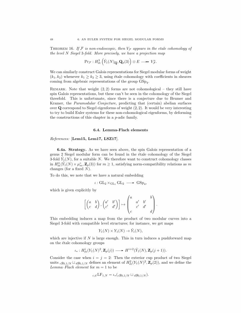
48 6. AN EULER SYSTEM FOR SIEGEL MODULAR FORMS
Theorem 16. If F is non-endoscopic, then VF appears in the etale cohomology ofthe level N Siegel 3-fold. More precisely, we have a projection map
PrF : H3et
(Y1(N)Q,Qp(3)
)⊗ E -- V ∗F .
We can similarly construct Galois representations for Siegel modular forms of weight(k1, k2) whenever k1 ≥ k2 ≥ 3, using etale cohomology with coefficients in sheavescoming from algebraic representations of the group GSp4.
Remark. Note that weight (2, 2) forms are not cohomological – they still havespin Galois representations, but these can’t be seen in the cohomology of the Siegelthreefold. This is unfortunate, since there is a conjecture due to Brumer andKramer, the Paramodular Conjecture, predicting that (certain) abelian surfacesover Q correspond to Siegel eigenforms of weight (2, 2). It would be very interestingto try to build Euler systems for these non-cohomological eigenforms, by deformingthe constructions of this chapter in a p-adic family. �
6.4. Lemma-Flach elements
References: [Lem15, Lem17, LSZ17].
6.4a. Strategy. As we have seen above, the spin Galois representation of agenus 2 Siegel modular form can be found in the etale cohomology of the Siegel3-fold Y1(N), for a suitable N . We therefore want to construct cohomology classes
in H4et(Y1(N)× µ◦m,Zp(3)) for m ≥ 1, satisfying norm-compatibility relations as m
changes (for a fixed N).
To do this, we note that we have a natural embedding
ι : GL2×GL1GL2
- GSp4,
which is given explicitly by
[(a bc d
),
(a′ b′
c′ d′
)]7→
a b
a′ b′
c′ d′
c d
.
This embedding induces a map from the product of two modular curves into aSiegel 3-fold with compatible level structures; for instance, we get maps
Y1(N)× Y1(N)→ Y1(N),
which are injective if N is large enough. This in turn induces a pushforward mapon the etale cohomology groups
ι∗ : Hiet(Y1(N)2,Zp(j)) - Hi+2(Y1(N),Zp(j + 1)).
Consider the case when i = j = 2: Then the exterior cup product of two Siegelunits cg0,1/N t dg0,1/N defines an element of H2
et(Y1(N)2,Zp(2)), and we define theLemma–Flach element for m = 1 to be
c,d LF1,N = ι∗(cg0,1/N t dg0,1/N ).

6.4. LEMMA-FLACH ELEMENTS 49
6.4b. Motivation: integral formulae. As in Chapter 3 above, there is agood motivation for why this class c,d LF1,N should be interesting.
There is an integral formula for the spin L-function of GSp4, which is due toPiatetskii-Shapiro. If F is a non-endoscopic, holomorphic eigenform of weight (3, 3)(or of any cohomological weight), then we can consider the integral∫
(Γ1(N)\H)2E(τ1, s)E(τ2, s)F(τ1, τ2)dA
where E(τ, s) is a suitably-chosen family of Eisenstein series, and dA = dτ1∧dτ1∧dτ2∧dτ2=(τ1)=(τ2)
is the invariant measure on (Γ1(N)\H)2. The general theory tells us that thisunfolds into a product of local integrals, and the local integral at a finite placecomputes the spin L-factor.
The problem is that the local integral at ∞ is always zero! This can be fixed byreplacing the holomorphic eigenform F with an “evil twin” Fg, which is a real-analytic but non-holomorphic function on Y1(N)(C) with the same Hecke eigenval-ues as F ; this doesn’t change the local integrals at the finite places, but gives us anon-vanishing archimedean integral.
As in the Rankin–Selberg setting, the Lemma–Flach class we’ve defined is naturallythe image under the etale regulator of a motivic cohomology class. The main resultof [Lem17] shows that the Beilinson regulator of this motivic class, paired with
an appropriate differential on Y1(N)(C) coming from Fg, gives Piatetskii-Shapiro’sintegral for Lspin(F , s) at s = − 1
2 .
Remark. The g stands for “generic”. Representation-theoretically, the problemis that the discrete-series representations of GSp4(R) come in pairs (“local L-packets”), consisting of a holomorphic representation and a non-holomorphic one,and it is the non-holomorphic one which is generic (admits a Whittaker model) andthus can contribute to the integral formula.
One can also replace Y1(N)×Y1(N) with a symmetric space associated to GL2 /K,where K is an imaginary quadratic field; this gives an alternative integral represen-tation which does involve the holomorphic eigenform F . However, it seems to beimpossible to interpret this integral as the regulator of a motivic cohomology class,since the symmetric space for GL2 /K is not an algebraic variety. �
6.4c. Lemma–Eisenstein classes. Our task is now to extend this to anEuler system: that is, to define classes c,d LFm,N for m > 1 satisfying good norm-compatibility properties. As before, we’ll start by defining classes on higher-levelmodular varities, which are easier to work with, and proving norm-compatibilityrelations for these auxiliary classes.
Let us define U(M,N) ={γ ∈ GSp4(Z) : γ =
(I2 02
02 I2
)mod (M M
N N )}
, and Y (M,N)
the corresponding Siegel threefold.
Lemma 1. If M |N , the group U(M,N) is normalised by the element u =
(1 1
1 11
1
).
Define ιM,N : Y (M,N)2 → Y (M,N) to be the composite
Y (M,N)2 ⊂ι- Y (M,N)
u- Y (M,N).

50 6. AN EULER SYSTEM FOR SIEGEL MODULAR FORMS
Here, Y (M,N)2 denotes as above the fibre product of two copies of Y (M,N) overµ◦M .
Definition. The Lemma-Eisenstein class c,d LEisM,N is the image of cg0,1/N tdg0,1/N under (ιM,N )∗. Here, we regard cg0,1/Ntdg0,1/N as an element of H2
et(Y (M,N)2,Zp(2))via pullback.
6.4d. Norm relations. Exactly as before, one sees straightforwardly that theLemma–Eisenstein classes satisfy norm relations as N changes.
Proposition 9. Suppose that M |N and ` is a prime with ` | N . Then
(pr1)∗(c,d LEisM,`N ) = c,d LEisM,N ,
where pr1 is the natural quotient map Y (M,N`)→ Y (M,N). �
(Exercise: formulate and prove a similar formula for ` - N .)
The second norm relation: changing M . Let us write τ` for the “non-standard”degeneracy map Y (`M,N) to Y (M,N), given by the right-translation action of(``
11
)∈ GSp4(Q`) ⊂ GSp4(Af ). Note that τ` factors as
Y (`M,N) - Y (M(`), N)π2,`- Y (M,N),
where the first map is the natural degeneracy map.
Theorem 17. Suppose `|M and `M | N . Then we have
(τ`)∗ (c,d LEis`M,N ) = U ′` · c,d LEisM,N .
Here, U ′` is the Hecke correspondence on Y (M,N) given by the element of GSp4(Af )
which is
(``
11
)at `, and the identity elsewhere.
Remark. Again, there is a similar but slightly more complicated formula in thecase when ` -M (but still `M | N). �

6.4. LEMMA-FLACH ELEMENTS 51
Proof. We erect the following commutative diagram, in which all verticalarrows are the natural degeneracy maps:
Y (`M,N)2 ⊂ι`M,N- Y (`M,N)
Y (`M,N)2
wwwwwwwwwwwwwwwwww- Y (M(`), N))
?
♦
Y (M,N)2?
⊂ιM,N - Y (M,N)
π1,`
?
Y (M,N)
τ`
-
π2,`
-
We claim that the middle arrow is actually injective. This is equivalent to the claimthat
H(Af ) ∩ uU(M(`), N)u−1 = U(M`,N)2,
which is an easy matrix computation.
When ` | M , we see that the square marked ♦ has both horizontal arrows closedimmersions, and both vertical arrows of degree `3. So it is Cartesian, and wemay conclude that the image of c,d LEis`M,N under pushforward to Y (M(`), N)coincides with the pullback of c,d LEisM,N . The result now follows by pushingboth of these elements forward along the diagonal arrow and observing that U ′` =(π2,`)∗ ◦ (π1,`)
∗. �
6.4e. Lemma-Flach classes and their norm relations. Let m ≥ 1. Welet $m denote the element of A×f whose `-th component is `v`(m). Then right
translation by the element
($m
$m1
1
)∈ GSp4(Af ) induces a map
sm : Y (m,mN)→ Y1(N)× µ◦m.
Definition. We define the Lemma-Flach element c,d LFm,N to be the image of
c,d LEism,mN under (sm)∗.
Theorem 18. Let ` be prime such that `|M and `|N . Then we have
normQ(µ`m)Q(µm) (c,d LF`m,N ) = U ′` · c,d LFm,N .
Proof. Analogous to the proof of the corresponding statement for Beilinson–Flach elements. �


CHAPTER 7
Projects
7.1. An Euler system for GSp4×GL2
The goal of this project is to construct an Euler system for the Galois represen-tations appearing in the cohomology of a certain 4-dimensional Shimura variety:namely, the product of a Siegel modular threefold and a modular curve.
The underlying Rankin–Selberg formula (in the sense of Section 3.3) was proven byNovodvorsky [Nov79]: it uses the embedding ι : GL2×GL1
GL2 ↪→ GSp4×GL1GL2
given by
((a bc d
),
(a′ b′
c′ d′
))7→
a b
a′ b′
c′ d′
c d
,
(a′ b′
c′ d′
) .Novodvorsky’s formula expresses values of the degree 8 L-function of an automor-phic form F for GSp4×GL1
GL2 in terms of an integal over GL2×GL1GL2; roughly,
one integrates ι∗($F ), where $F is a certain differential associated to F , againstan Eisenstein series on the first GL2 factor of GL2×GL2.
The corresponding Euler system should roughly be constructed as follows: let Y bea modular curve, and let gY be a Siegel unit on Y . Its image under the Kummermap κp(gY ) is an element of H1
et(Y,Qp(1)). We can regard it as an element ofH1
et(Y × Y,Qp(1)) via pullback along the natural projection map Y × Y → Y ontothe first factor. Then the bottom class of the Euler system (with trivial coefficients)should be given by
ι∗(κp(gY )) ∈ H5et(S × Y,Qp(3)),
where S denotes a Siegel 3-fold of a suitable level.
Remark. As in Section 3.3, this is visibly the etale regulator of a motivic class,whose Beilinson regulator is a special value of Novodvorsky’s integral. �
The aim of the project is to show that the methods of Chapters 4 and 6 can beadapted to give an Euler system of GSp4×GL2.
This project has several sub-projects, which are to some extent orthogonal (so itwould be suitable for a fairly large team):
• Writing down the relevant cohomology classes over the cyclotomic exten-sions of Q, using suitable level structures on Y and S.
• Proving norm-compatibility statements in the “vertical” aspect (i.e. prov-ing a relation under the Galois corestriction map for the the classes overQ(µpn+1) and Q(µpn) where p is a prime and n ≥ 1). This ought to be
53

54 7. PROJECTS
possible using a “Cartesian square” diagram analogous to those we hadabove for the Beilinson–Flach and Lemma–Flach elements.
• Proving the “horizontal” (or tame) norm relation (i.e. proving a relationunder the Galois corestriction map for the classes over Q(µm`) and Q(µm),where ` is a prime not dividing m. This is a rather more difficult problem,since extra Euler factors make an appearance, and we did not discuss itin these lecture notes. In [LLZ14] and [KLZ17], we proved these normrelations by explicit computations, but this method does not generalizeeasily. A different and much more flexible approach for proving the tamenorm relations (using local zeta integrals) was developed in the GSp4-casein [LSZ17, §§3, 10], and this strategy should generalize1 to GSp4×GL2.
• studying the case of higher weights (i.e. determining for which coefficientsystems F on S × Y one can construct elements in H5
et(S × Y,F (3))).The corresponding calculation for the GSp4-case can be found in [LSZ17,§§4, 8].
7.2. Euler systems and Selmer groups in Coleman families
Modular forms can often be deformed in p-adic families (Hida families of ordinaryforms, or the more general finite-slope families constructed by Coleman [Col97]).One knows that the Euler system of Kato, and the Euler system of Beilinson–Flachelements, can be interpolated in Coleman families (see [Wan14], [Han15] for theformer, and [LZ16] for the latter). This raises (at least) two natural questions.
• In the Beilinson–Flach setting, can one define a Selmer group attached tothe family, and use the Euler system to give upper bounds on its size?There is a general approach to defining Selmer groups in families, due toPottharst [Pot13], and it would be interesting to try to formulate andprove a bound for Pottharst’s Selmer groups in this setting.
• Are there analogous interpolation results for other Euler systems, e.g. inthe Hilbert or Siegel settings? The existence of Hida families in thesesettings is well-known ([Hid89, TU99]), so as a first step one could showthat the Euler systems vary in these families.
Andreatta, Iovita and Pilloni have recently shown the existence of p-adic families of finite-slope automorphic forms in both the Hilbert [AIP16]and the Siegel case [AIP15]; but whether the Euler systems interpolatein these families is an open question.
1It is possible to give a new proof of the tame norm relations for Beilinson–Flach elementsusing local zeta integrals. This is currently being worked out by Giada Grossi.

Bibliography
[AIP15] Fabrizio Andreatta, Adrian Iovita, and Vincent Pilloni, p-adic families of Siegel mod-
ular cuspforms, Ann. of Math. (2) 181 (2015), no. 2, 623–697. MR 3275848 ↑ 54[AIP16] , On overconvergent Hilbert modular cusp forms, Asterisque (2016), no. 382,
163–193. MR 3581177 ↑ 54
[And87] Anatolij N. Andrianov, Quadratic forms and Hecke operators, Grundlehren der Mathe-matischen Wissenschaften [Fundamental Principles of Mathematical Sciences], vol. 286,
Springer-Verlag, Berlin, 1987. MR 884891 ↑ 46
[Beı84] A. A. Beılinson, Higher regulators and values of L-functions, Current problems inmathematics, Vol. 24, Itogi Nauki i Tekhniki, Akad. Nauk SSSR, Vsesoyuz. Inst.
Nauchn. i Tekhn. Inform., Moscow, 1984, pp. 181–238. MR 760999 ↑ 26[BDR15] Massimo Bertolini, Henri Darmon, and Victor Rotger, Beilinson–Flach elements and
Euler systems I: syntomic regulators and p-adic Rankin L-series, J. Algebraic Geom.
24 (2015), no. 2, 355–378. MR 3311587 ↑ 29[Bes00] Amnon Besser, Syntomic regulators and p-adic integration. I. Rigid syntomic regula-
tors, Israel J. Math. 120 (2000), no. 1, 291–334. MR 1809626 ↑ 29
[Bes12] , On the syntomic regulator for K1 of a surface, Israel J. Math. 190 (2012),no. 1, 29–66. MR 2956231 ↑ 29
[Bum05] Daniel Bump, The Rankin-Selberg method: an introduction and survey, Automorphic
representations, L-functions and applications: progress and prospects, Ohio State Univ.Math. Res. Inst. Publ., vol. 11, de Gruyter, Berlin, 2005, pp. 41–73. MR 2192819 ↑ 27
[CR18] Antonio Cauchi and Joaquin Rodrigues, Euler systems for GSp(6), in preparation,
2018. ↑ 28[CRSS15] John Coates, A. Raghuram, Anupam Saikia, and R. Sujatha (eds.), The Bloch-Kato
conjecture for the Riemann zeta function, London Mathematical Society Lecture NoteSeries, vol. 418, Cambridge University Press, Cambridge, 2015. MR 3410209 ↑ 15
[Col97] Robert F. Coleman, p-adic Banach spaces and families of modular forms, Invent.
Math. 127 (1997), no. 3, 417–479. MR 1431135 ↑ 54[DDT97] Henri Darmon, Fred Diamond, and Richard Taylor, Fermat’s last theorem, Elliptic
curves, modular forms & Fermat’s last theorem (Hong Kong, 1993), Int. Press, Cam-
bridge, MA, 1997, pp. 2–140. MR 1605752 ↑ 18[DS05] Fred Diamond and Jerry Shurman, A first course in modular forms, Graduate Texts
in Mathematics, vol. 228, Springer-Verlag, New York, 2005. MR 2112196 ↑ 18
[Gea06] Matthew Thomas Gealy, On the Tamagawa Number Conjecture for motives attachedto modular forms, Caltech PhD thesis, 2006. ↑ 42
[Han15] David Hansen, Iwasawa theory of overconvergent modular forms, preprint, 2015. ↑ 54[Hid89] Haruzo Hida, On nearly ordinary Hecke algebras for GL(2) over totally real fields,
Algebraic number theory, Adv. Stud. Pure Math., vol. 17, Academic Press, Boston,
MA, 1989, pp. 139–169. MR 1097614 ↑ 54[Jan88] Uwe Jannsen, Continuous etale cohomology, Math. Ann. 280 (1988), no. 2, 207–245.
MR 929536 ↑ 17
[Kat04] Kazuya Kato, P -adic Hodge theory and values of zeta functions of modularforms, Asterisque 295 (2004), ix, 117–290, Cohomologies p-adiques et applications
arithmetiques. III. MR 2104361 ↑ 13, 20, 22, 23
[KLZ15] Guido Kings, David Loeffler, and Sarah Livia Zerbes, Rankin–Eisenstein classes formodular forms, to appear, 2015, arXiv:1501.03289. ↑ 31
[KLZ17] , Rankin–Eisenstein classes and explicit reciprocity laws, Cambridge J Math 5(2017), no. 1, 1–122. ↑ 31, 41, 42, 54
55

56 BIBLIOGRAPHY
[Kol91] V. A. Kolyvagin, On the structure of Shafarevich-Tate groups, Algebraic geometry
(Chicago, IL, 1989), Lecture Notes in Math., vol. 1479, Springer, Berlin, 1991, pp. 94–
121. MR 1181210 ↑ 13, 20[Lan91] Steven E. Landsburg, Relative Chow groups, Illinois J. Math. 35 (1991), no. 4, 618–641.
MR 1115990 ↑ 26
[Lan87] Serge Lang, Elliptic functions, second ed., Graduate Texts in Mathematics, vol. 112,Springer-Verlag, New York, 1987, With an appendix by J. Tate. MR 890960 ↑ 22
[LLZ14] Antonio Lei, David Loeffler, and Sarah Livia Zerbes, Euler systems for Rankin–
Selberg convolutions of modular forms, Ann. of Math. (2) 180 (2014), no. 2, 653–771.MR 3224721 ↑ 31, 54
[LLZ16] , Euler systems for Hilbert modular surfaces, preprint, 2016, arXiv:1607.07813.
↑ 28[Lem15] Francesco Lemma, On higher regulators of Siegel threefolds I: The vanishing on the
boundary, Asian J. Math. 19 (2015), no. 1, 83–120. MR 3318014 ↑ 48[Lem17] , On higher regulators of Siegel threefolds II: the connection to the special value,
Compos. Math. 153 (2017), no. 5, 889–946. MR 3705247 ↑ 48, 49
[LSZ17] David Loeffler, Christopher Skinner, and Sarah Livia Zerbes, Euler systems for GSp(4),preprint, 2017, arXiv:1706.00201. ↑ 28, 45, 48, 54
[LZ16] David Loeffler and Sarah Livia Zerbes, Rankin–Eisenstein classes in Coleman families,
Res. Math. Sci. 3 (2016), no. 29, special collection in honour of Robert F. Coleman. ↑54
[MR04] Barry Mazur and Karl Rubin, Introduction to Kolyvagin systems, Stark’s conjectures:
recent work and new directions, Contemp. Math., vol. 358, Amer. Math. Soc., Provi-dence, RI, 2004, pp. 207–221. MR 2088718 ↑ 12
[MVW06] Carlo Mazza, Vladimir Voevodsky, and Charles Weibel, Lecture notes on motivic co-
homology, Clay Mathematics Monographs, vol. 2, American Mathematical Society,Providence, RI; Clay Mathematics Institute, Cambridge, MA, 2006. MR 2242284 ↑ 26
[Nek98] Jan Nekovar, Syntomic cohomology and p-adic regulators, preprint, 1998. ↑ 29[NN16] Jan Nekovar and Wies lawa Nizio l, Syntomic cohomology and p-adic regulators for
varieties over p-adic fields, Algebra Number Theory 10 (2016), no. 8, 1695–1790,
With appendices by Laurent Berger and Frederic Deglise. MR 3556797 ↑ 29[Niz97] Wies lawa Nizio l, On the image of p-adic regulators, Invent. Math. 127 (1997), no. 2,
375–400. MR 1427624 ↑ 29
[Nov79] Mark Novodvorsky, Automorphic L-functions for the symplectic group GSp(4), Auto-morphic forms, representations and L-functions (Corvallis, 1977) (Armand Borel and
William Casselman, eds.), Proc. Sympos. Pure Math, vol. 33 Part 2, Amer. Math. Soc.,
1979, pp. 87–95. ↑ 53[PS97] I. I. Piatetski-Shapiro, L-functions for GSp4, Pacific J. Math. (1997), no. Special Issue,
259–275, Olga Taussky-Todd: in memoriam. MR 1610879 ↑ 47
[Pot13] Jonathan Pottharst, Analytic families of finite-slope Selmer groups, Algebra NumberTheory 7 (2013), no. 7, 1571–1612. MR 3117501 ↑ 54
[Rub00] Karl Rubin, Euler systems, Annals of Mathematics Studies, vol. 147, Princeton Univ.Press, 2000. MR 1749177 ↑ 12, 13, 14
[Tha88] Francisco Thaine, On the ideal class groups of real abelian number fields, Ann. of Math.(2) 128 (1988), no. 1, 1–18. MR 951505 ↑ 13
[TU99] J. Tilouine and E. Urban, Several-variable p-adic families of Siegel–Hilbert cusp eigen-
systems and their Galois representations, Ann. Sci. Ecole Norm. Sup. (4) 32 (1999),no. 4, 499–574. MR 1693583 ↑ 54
[vdG08] Gerard van der Geer, Siegel modular forms and their applications, The 1-2-3 of modular
forms, Universitext, Springer, Berlin, 2008, pp. 181–245. MR 2409679 ↑ 46[Wan14] Shanwen Wang, Le systeme d’Euler de Kato en famille (I), Comment. Math. Helv. 89
(2014), no. 4, 819–865. MR 3284296 ↑ 54
[Wei05] Rainer Weissauer, Four dimensional Galois representations, Asterisque 302 (2005),67–150, Formes automorphes. II. Le cas du groupe GSp(4). MR 2234860 ↑ 47