eu and developing countries: what is the impact of
TRANSCRIPT

1
EU and developing countries: what is the impact of agricultural preferences?♦♦♦♦
BY: MARIA CIPOLLINA
LUCA SALVATICI
University of Molise, Campobasso, Italy
Contact: Luca Salvatici
E-mail:[email protected]
Postal: University of Molise, via De Sanctis, 86100 Campobasso, Italy
Phone: (+39)08744240
Fax: (+39)0874311124
Co-Auth: Maria Cipollina
E-mail: [email protected]
Postal: University of Molise, via De Sanctis, 86100 Campobasso, Italy
Phone: (+39)08744041
Fax: (+39)0874311124
Date: June 2008
♦ This work was financially backed by the ‘Agricultural Trade Agreements (TRADEAG)’ project, funded by the European Commission (Specific Targeted Research Project, Contract no. 513666).

2
European Union and developing countries: what is the impact of agricultural
preferences?
Abstract
We assess the impact on trade of European Union (EU) preferences in the agricultural sector using a
gravity approach. We use trade statistics at the 6-digit level and compute an explicit measure of the
intensity of the preference margins showing the bias implied by the use of aggregate EU imports. As
far as the estimation method is concerned, we consider the potential selection bias implied by the
presence of zero-trade flows. Our results confirm an overall positive impact of preferences on trade
although with significant differences across products.
Keywords: Preferential Trade Policy; Agricultural Trade; Gravity Model.
1. Introduction
This work provides an analysis of the impact on trade of European Union (EU)
preferences in the agricultural sector. The analysis refers to imports from developing
countries to 15 “old” EU members in 2004. It is well-known that the EU has been increasing
its use of preferential regimes in order to promote economic development as well as the
integration of developing countries in the world economy. In this respect, the agricultural
sector plays a crucial role since it accounts for a large share of developing countries’
economies and is highly protected in the European market.
In section 2, we briefly review the literature that has analysed the impact of these policies.
From a methodological point of view, the commonly used econometric approach is based on
the gravitational model based on Newton’s Law of Gravitation that predicts that the volume
of trade between two economies increases with their size, measured as real GDP, population
or land area, and decreases with transaction costs measured as bilateral distance, adjacency or
cultural similarities (Baldwin, 1994; Eichengreen and Irwin, 1996; Feenstra, 1998; Anderson
and van Wincoop, 2003).
Following Anderson (1979) and Anderson and van Wincoop (2003) we derive a
theoretically grounded gravity equation where the trade cost factor depends on bilateral
distances, tariffs and preferential margins (Section 3). In the literature, preferential policies
are usually introduced as a dummy variable with value “1” if the exporting country belongs to

3
a preferential agreement and “0” if not whereas we use an explicit measure of the intensity of
the preference margins at the 6-digit tariff line level. The preference margin for each product
is calculated on a bilateral basis as the difference between the maximum applied duty by the
EU across all exporters and the duty faced by a specific exporter. This means that rather than
looking at the difference between multilateral (“bound”) tariffs and bilateral (applied) duties,
we focus on the actual preference margin with respect to possible competitors. Accordingly,
we avoid an overestimation of the competitive advantage enjoyed by the exporting country as
would be the case if the highest applied duties were lower than the maximum ceiling allowed
by the World Trade Organization (WTO) commitments.
Moreover, the assessment of the impact of trade preferences should be carried out using
disaggregated data rather than total exports as any discriminatory trade agreement applies at
product level: disaggregated data allows a more accurate analysis of policies that vary across
products (Agostino et al., 2007). On the other hand, the use of disaggregated data leads to two
types of shortcomings: (i) the elevated percentage of “zero trade flows” that creates obvious
problems in the log-linear form of the gravitational equation; (ii) the impossibility, for some
variables to obtain information at the detailed level at which tariff lines are specified.
In order to avoid the bias that would be implied by the drop of the observations with zero
flows, we implement the Heckman two-step procedure in line with the best practices in the
literature (Helpman et al., 2007; Linders and de Groot, 2006; Martin and Pham, 2008). The
choice of this procedure is not only instrumental in correcting possible biases but the results
of the first step that express the probability of registering a positive trade flow also allow us to
distinguish the impact of preferences on the number of traded goods (extensive margin) as
well as on the quantities traded (intensive margin). Extensive and intensive margins are worth
exploring since a large amount of recent literature considers the “quality” of traded goods,
understood as variety/diversification of exports, an important factor in explaining productivity
growth of the exporting country (Feenstra, 1994; Feenstra and Markusen, 1996; Feenstra et
al., 1999; Funke and Ruhwedel, 2001a and 2001b; Broda and Weinstein, 2006; Feenstra and
Kee, 2004a and 2004b).
As far as the lack of data is concerned, in order to control unobservable country and
product heterogeneity, we introduce product-by-exporter country and country-specific fixed
effects.
We estimate cross-sectional models for data on imports of 689 agricultural products from
161 Developing Countries (DCs) to 15 EU members provided by the MAcMap-HS6 database

4
and by Eurostat database COMEXT for 2004 (Section 4).1 The sensitivity of the results to
different levels of geographical aggregation for the importing region is explored considering
the 15 EU countries either individually or as an aggregate.
Results confirm that preferential regimes produce positive impacts both on the probability
of trade (extensive margin) and trade intensity (intensive margin) although they describe a
picture in which preferential regimes have very different impacts across products. However,
we show that both the geographical aggregation of the importing region and the use of
preferential policies dummies lead to an overestimation of the impact (Section 5).
2. EU Trade Policy and the developing countries: a brief survey of literature
The EU is engaged in a web of preferential trade relations with other countries or regional
groupings which range from the regular Generalized System of Preferences (GSP) to specific
provisions for LDCs (i.e. the Everything But Arms – EBA – initiative), the Africa-Caribbean-
Pacific agreement (i.e. the Lomé/Cotonou agreements) and the Bilateral Euro-Mediterranean
Association Agreements.2
In 2004 the EU GSP scheme included three main categories of benefits: the General
Scheme, first introduced in 1971, offering access to its markets at lower or zero tariffs to
imports from developing countries, the EBA initiative granting to the LDCs duty-free access
on all products with the exception of arms and munitions and the “GSP-plus” providing tariff
reductions and exemptions for developing countries that implement international conventions
on human and labour rights, environmental protection, fight against drugs, and good
governance.
The regular GSP covered around 7000 tariff lines where products were classified into two
groups according to the depth of the tariff cuts 3300 non-sensitive products were given duty-
free market access and 3700 sensitive products (including most agricultural products) with a
flat rate reduction of 3.5 percentage points from the Most Favoured Nation (MFN) duty.
The EBA considerably improved the extent of the preferential market access granted to
LDCs. Since 2002, as a matter of fact, duty-free access has been extended without any
quantitative restrictions to all products except for arms and three sensitive products, namely
bananas, rice and sugar (for these products a transition arrangement is to be provided until
2009). The EBA follows the same rules of origin specified in the GSP. This is seen as a major
1 In 2004, 178 countries benefitted from the EU preferential policy but data is not available for all of them. 2 For a detailed analysis of these preferential schemes see Bureau et al. (2004) and Gallezot (2005).

5
restriction to exporting processed products under the EBA especially for small countries that
find it difficult to find all components of their products within their boundaries (Bureau et al.,
2004). According to De Maria et al. (2008), in 2004, the percentage of agro-food tariff lines
covered by the GSP, EBA and GSP-plus were 45%, 68% and 99% respectively.
The Cotonou Partnership Agreement includes preferences and linkages between trade and
financial assistance for over 70 ACP countries which are mostly former colonies of the EU
Member States. The agreements constitute a follow-up to the Yaoundé and Lomé
Conventions which provided non-reciprocal trade benefits in 99 percent of industrial goods
and some agricultural products.3 The Lomé preferences expired at the end of 2007 except for
LDCs, and the EU signed full Economic Partnership Agreements (EPAs) with the Caribbean
region as well as interim agreements with African and Pacific countries. EPAs fully open up
the EU market to these countries and allow for gradual liberalisation over many years on the
ACP side. They also include chapters on development cooperation, revised rules of origin to
make it easier to trade with the EU and other issues.
The EU also has bilateral arrangements with 10 Mediterranean countries. The Euro-
Mediterranean partnership was launched at the 1995 Barcelona Conference which forecasted
a free trade area by 2010. The Bilateral Euro-Mediterranean Association Agreements are a
first step in this direction. Some of these agreements allow non-reciprocal free access for non-
sensitive products into the EU market and progressive liberalization for other products.
The literature on trade preferences focuses on two main issues: (i) the value of
preferences, and (ii) their impact on trade.
Many studies measure the value of preferences, i.e. the benefit that receiving countries
might draw from trade preferences (Alexandraki and Lankes, 2004; Bouët et al., 2005;
Candau and Jean, 2005). Under simplifying assumptions (perfect substitutability across
origins and constant world prices, in particular), a simple calculation of the value of the rent
(Vj) arising from preferential tariff duties for any partner j can be carried out:
∑ −=i
pref
ijijijij utilMprefmfnV )( (1)
where i is the tariff line, mfn and pref are respectively the MFN and the preferential applied
tariff duty, M refers to a country’s dutiable imports of product i from partner j, and util is the
corresponding utilisation rate (i.e. the ratio of exports under the EBA to exports eligible to the
3 Agricultural preferences include processed fruits and vegetables, corn, beef, rice, onions, tomatoes, strawberries, citrus fruit, tobacco and bananas.

6
EBA). Using this measure, Candau and Jean (2005) find that EU tariff preferences are an
important stake for a number of developing countries, in particular in sub-Saharan Africa: for
all country groups except the GSP-only countries, they represent a significant proportion of
the value of dutiable exports to the EU (up to 10% for sub-Saharan African countries and
LDCs).
Given the relevance of the utilisation rate of preferences in the calculation of the value of
the rent (Vj) arising from preferential tariff duties for any partner, it is not surprising that the
utilization rate has attracted a substantial body of research (Brenton, 2003; Bureau et al, 2004;
Manchin, 2005; Mold, 2004; Stevens and Kennan, 2004; Anson e al., 2005; Augier et al.,
2005; Estevadeordal and Suominen, 2005; Candau and Jean, 2005). It has been argued that
the use of some schemes is limited by stringent rules of origin and administrative
complications that make it very difficult for exporters to comply with the scheme’s
requirements (Gallezot and Bureau, 2004; Stevens and Kennan, 2004; Candau and Jean,
2005). By focusing on each agreement separately, it can be seen that the rate of utilization is
quite low: for example, the rate of utilization of EBA does not exceed 18% on average and the
rate of utilization of the EU GSP scheme for non-LDCs is also relatively low. However, it has
been pointed out that DC exports are often eligible for several preference schemes so that not
all of them can be filled at the same time (Bureau et al, 2004).
As far as the impact on trade is concerned, most of the literature relies on gravity models,
based on Newton’s Law of Gravitation, that predict that the volume of trade, Mij, between two
economies increases with their size, Yi(j) (proxies are real GDP, population, land area),
decreases with transaction costs measured as bilateral distance, dij, adjacency and intensifies
with preferential trade agreements and other factors such as a common language or colonial
ties (Anderson, 1979; Anderson and van Wincoop, 2003). Typically, the stochastic version of
the gravity equation has the form:
Mij = α0Y i α1
Y j α2
d ij α3
εij (2)
where εij is an error term with E(εij |Yi, Yj, dij) = 1, assumed to be statistically independent of
the regressors.
Most of the estimates are obtained from cross-country regressions. Even if panel data pins
down the estimates of persistent effects more accurately, only very recently gravity equations
have been estimated using panel data techniques (Yeyati, 2003; Ghosh, Yamarik, 2004; Rose,
2004a, b; Carrère, 2006; and others). In this respect, it is worth recalling that equation (2),

7
derived under the assumption of symmetric and constant bilateral trade costs, only holds with
cross section data.
Most of the empirical analyses use gravitational models with aggregated data both in
terms of products and in terms of countries. As far as the product aggregation is concerned, it
seems awkward to use aggregate export flows to analyse the effects of trade preferences
applied at product level. Indeed, the few works using disaggregated data confirm that
aggregation produces a significant estimation bias (Manchin, 2005; Agostino et al., 2007).
On the contrary, the only mention of the geographical aggregation issue we are aware of is
provided by Engel (2002) who criticizes the use of elasticities of substitution estimated
without considering the number of countries involved. By comparing the results for the EU15
as a whole with those obtained taking into account the differences in the import structure of
the 15 EU members, we provide a first time assessment of this type of bias.
The use of disaggregated data implies the presence of a high percentage of “zero trade
flows”. These zero observations pose no problem for the estimation of gravity equations in
their multiplicative form but they raise a problem in the log-linear specification of the gravity
equation that is usually adopted:
ln (Mij) = ln(α0) + α1 ln (Yi) + α2 ln (Yj) + α3 ln (dij) + εij. (3).
In many cases, the solution is simply to drop the pairs with zero trade from the data set
and estimate the log-linear form by OLS. Even without mentioning the fact that the omission
of zero flows could strongly reduce the sample and lead to a considerable loss of information,
limiting the analysis to observations where bilateral trade flows are positive is a significant
source of bias since the selected sample is not random.4 Zeros may be the result of rounding
errors. If trade is measured in thousands of dollars, for pairs of countries in which bilateral
trade did not reach a minimum value, the value of trade may be registered as zero. If these
rounded-down observations are partially compensated by rounded-up ones, the overall effect
of these errors will be relatively minor. However, rounding down is more likely to occur for
small or distant countries and the probability of rounding down will therefore depend on the
value of the covariates leading to the inconsistency of the estimators. The zeros can also be
missing observations which are wrongly recorded as zero. This problem is more likely to
occur when small countries are considered and, again, measurement error will depend on the
covariates leading to inconsistency.
4 For a general discussion of the selection bias problem see Wooldridge (2002, cap. 17).

8
When the dependent variable is zero for a substantial part of the sample but positive for
the rest of the sample, the econometric theory suggests the use of Tobit models. As is typical
in the literature, many gravity works perform Tobit estimates by constructing a new
dependent variable y = ln(1+Mij). However, this procedure relies on rather restrictive
assumptions that are not likely to hold since the censoring at zero is not a “simple”
consequence of the fact that trade cannot be negative. Zero flows, as a matter of fact, do not
reflect unobservable trade values but they are the result of economic decision-making based
on the potential profitability of engaging in bilateral trade at all.
Some authors suggest the Poisson Quasi Maximum Likelihood (PQML) estimator as a
way of dealing with the question of ‘zeros’ in the trade matrix in order to get unbiased and
consistent estimates. Santos Silva and Tenreyro (2005) strongly recommend that gravity type
models in particular as well as other constant-elasticity models in general should be estimated
in the multiplicative form and suggest a simple quasi-maximum likelihood estimation
technique based on Poisson regression (Siliverstovs and Schumacher, 2007).
A recent work by Martin and Pham (2008) uses Monte Carlo generated data in order to
investigate the performance of different estimators. It appears that the Poisson estimator turns
out to be severely biased while Heckman estimators perform well if true identifying
restrictions are available. Several recent works implement the Heckman (1979) two-stage
procedure (Linders and de Groot, 2006; Helpman et al., 2007). This approach, which takes
into account the information provided by zero-valued observations to get unbiased estimates,
is the one we are going to use in this work.
It is not an easy task to summarize the results of the large amount of literature that
assesses the impact of preferences on trade. The studies report very different estimates due to
the fact that they differ greatly in data sets, sample sizes, independent variables used in the
analysis and estimation methods. In any case, the expectation of the positive impact of
preferences on trade is by far and large confirmed.
With regard to the estimated coefficients of the impact of preferences, comprehensive
surveys of the estimated PTAs impact are provided by Nielsen (2003) and Cardamone (2007).
Many works focus specifically on the EU policies (Nilsson, 2002; Adam et al., 2003; Persson
and Wilhelmsson, 2005; Verdeja, 2006).
The EU GSP scheme does not seem to have a large impact since the import coefficient
ranges from 0.04 to 0.86 (Nilsson, 2002; Rose, 2004a; Persson and Wilhelmsson, 2005;
Verdeja, 2006), and some authors even find highly significant negative coefficients (Oguledo

9
and Macphee, 1994; Nilsson, 2002; Rose, 2004b; Subramanian and Wei, 2005). Looking at
the results for different sectors, Subramanian and Wei (2005) report positive estimates for the
clothing industry only whereas it is negative for the footwear and food industries.
Several studies (Carrère, 2004; Nilsson, 2005; Persson and Wilhelmsson, 2005; Agostino
et al., 2007) find that the EBA initiative provided a significant boost to LDCs’ exports.
Positive results have also been obtained for ACP countries, (Carrère, 2004, Nilsson, 2005;
Acosta-Rojas et al., 2005; Persson and Wilhelmsson, 2005; Persson, 2007, Verdeja (2006), as
well as for the Euro-Mediterranean agreements (Gaulier et al., 2004; Alvarez-Coque and
Martì-Selva, 2006; Pusterla, 2007) although the estimated impact sometimes seems
exceedingly high since coefficients range between 3.09 and 5.2 (Amurgo-Pacheco, 2006).
In the literature that assesses the impact of EU references on trade volumes from ACP
countries, it is worth mentioning the approach adopted by Manchin (2005) since it shares
several features with our work such as the use of highly detailed trade data, an explicit
measure of the preference margins, and the implementation of the Heckman two-step
procedure. The evidence provided confirms that preferences played a significant role in
improving market access to the EU in almost all sectors, with important differences across
sectors. However, these results are not directly comparable with ours since the preference
margin definitions differ and, more importantly, Manchin focuses on the utilization rates and
studies the factors which influence the decision to export using preferential schemes.
3. Gravity model
We follow Anderson (1979) and Anderson and van Wincoop (2003) in order construct our
gravity equation including many commodity classes of goods (denoted by k where k=1,2….K)
flowing between countries i and j. Consumption decisions are taken at two different levels: in
the first stage, the decision is how much to consume across product classes; in the second
stage, the decision is how much to import within a product class across countries of origin
(Armington assumption), so that bilateral trade is determined in “conditional general
equilibrium” whereby product markets for each good produced in each country clear
conditional on the observed output structure, Yjk, and expenditure allocations, Ejk.
The CES subutility function for product k and importer j facing i = 1…I exporting sources
can be written as follows:
[ ] kθ
ikθ
ijk
kθ
ikjk cβu/1
∑=− (4)

10
where cijk is the country j consumption for the commodity k importer from country i, βik is a
demand shifter which could represent unobserved differences in the number of distinct
varieties available from each exporter and kkk σσθ /)1( −= , with σk > 1 representing the
elasticity of substitution among all varieties from different exporters. Consumers maximize
their utility subject to:
jki ijkijk Ecp =∑ (5)
where Ejk is the country j’s expenditure for product class k.
Define the price index for commodity k in each country, Pjk, over the prices of individual
varieties produced in i and sold in j, pijk,
[ ] kσkσi ijkikjk pβP
−−∑=
1/11)( (6)
The imported good’s expenditure share is linked to its relative price by:
kσ
jk
ijkik
ijkP
pβφ
−
=
1
(7),
while the nominal demand for commodity k of country i by country j is:
j
kσ
jk
ijkik
jijkijkijkijk EP
pβEφcpm
−
===
1
(8).
Finally, using the national account identity between total expenditure (Ej) and total income
(Yj) we get:
j
kσ
jk
ijkik
ijk YP
pβm
−
=
1
(9).
Prices differ between locations due to trade costs. If pik denotes the exporter’s supply price
for commodity k, net of trade costs, and tikj is the trade cost factor between i and j for
commodity k so that pijk=piktijk, we get:
j
kσ
jk
ijkikik
ijk YP
tpβm
−
=
1
(10).
Moreover, if we assume that the production of commodity k for country i is a fraction of total
output, the market-clearing condition implies:
∑
=∑=
−
−
jj
kσ
jk
ijkkσikik
jijkiik Y
P
tpβmYφ
1
1)( (11).

11
Using the (11) to get the equilibrium scaled prices { ikik pβ } and substituting them in the
demand equation (10), we get:
( )( )∑
=−
−
jj
kσijkijk
jiikkσ
jkijk
ijkYPt
YYφPtm
1
1
/
/ (12)
If we define world national income by ∑=j jw YY , income shares by wjj YY=θ , the
exporter’s price index for good k by ∑≡ −−j
kσj
kσjkijkik θPtP
111 ))/( and assume that the trade
barriers are symmetric (that is, jikijk tt = ), we get the gravity equation:
kσ
jkik
ijk
w
jiik
ijkPP
t
Y
YYφm
−
=
1
(13).
Trade costs depend on transport costs, proxied by distance (dij), tariffs (τijk) imposed by
country j on imports of commodity k from country i, and preferential margins prefijk:
1)( −= ijkijijkijk prefdτt (14).
Finally, we can rewrite the gravity equation in (13) as:
kσ
ijkjkik
ijijk
w
jiik
ijkprefPP
dτ
Y
YYφm
−
=
1
(15),
or in the logarithmic form:
εPσPσprefσdστσφYYkm jkkikkijkkijkijkkikjiijk +−−−−−−−+−++++= ln)1(ln)1(ln)1(ln)1(ln)1(lnlnlnln
(16).
4. Econometric estimation
In order to estimate the impact of preferences on bilateral trade, we first have to decide
how to take into account the multilateral price terms, Pik. In the literature, three methods are
suggested: (1) the use of published data on price indexes (Bergstrand, 1985, 1989; Baier and
Bergstrand, 2001; Head and Mayer, 2000); (2) direct estimation à la Anderson and van
Wincoop (2003); (3) or the use of country fixed effects (Hummels, 1999; Rose and van
Wincoop, 2001; Eaton and Kortum, 2002; Feenstra, 2002; Redding and Venables, 2000).
The main weakness of the first method is that the existing price indexes may not
accurately reflect the true border effects (Feenstra, 2002). Consequently, Anderson and van
Wincoop (2003) estimate the structural equation with non-linear least squares after solving

12
the multilateral resistance indices according to the observables, i.e., bilateral distances and a
dummy variable for international borders. However, the computationally easier method for
accounting for multilateral price terms in cross section – that will also generate unbiased
coefficient estimates – is to estimate the gravity equation using country-specific fixed effects.
Since detailed data on consumption shares is not available, the only way to take into
account the unobserved shares, ϕik, is to include fixed effects for the k commodities from
country i. Let kΦ denote a dummy equal to “1” if imported good is commodity k, and “0” if
not; let i
1Φ denote a dummy equal to “1” if country i is the exporter, and “0” otherwise; and
let j
2Φ denote a dummy equal to “1” if country j is the importer, and “0” if not. Equation (16)
becomes:
εββprefσdστσβYYkm jjiiijkkijkijkk
kkjiijk +Φ+Φ+−+−+−+Φ+++= 2211 ln)1(ln)1(ln)1(lnlnln (17),
where the coefficients ikk φβ ln= , 1
1 )ln( −= kσik
iPβ and 1
2 )ln( −= kσjk
jPβ .
Estimates of coefficients are very sensitive to assumptions about the elasticity of
substitution (σk). Some authors (Feenstra, 1994; Eaton and Kortum, 2002) use data on prices
to estimate σk through the demand equation. Other authors estimate elasticity through the
gravity equations using information about directly observed trade barriers such as tariffs
and/or transport costs (Hummels, 2001; Baier and Bergstrand, 2001; Head and Ries, 2001). In
this respect, we do not attempt to provide original estimates but explore the sensitivity of the
results with respect to different values for σk. In order to choose the values, we follow
Anderson and van Wincoop (2004) who offer a review of methodologies used to estimate the
elasticity of substitution and conclude that the overall estimated σk is likely to be in the range
of 5 to 10.
As mentioned in Section 2, we address the issue of zero flows by adopting the Heckman
(1979) sample selection model. The Heckman two-step approach transforms a selection bias
problem into an omitted variable one solved by including an additional variable, the Mills
ratio, between the regressors.
The first stage consists of estimating a Probit equation that specifies the probability (ρ)
that country i exports product k to j according to observable variables:
ρijk = Pr ( *ijkM > 0 │observed variables) = Θ( )****
kijijkW κςξγ +++′ (18)

13
where ξ , ζ and κ are exporter, importer and product fixed effects, respectively. Θ(.) is the
cumulative distribution function of the unit-normal distribution, and every starred coefficient
represents the original coefficient divided by the standard deviation ση. Predicted components
of this equation are used to construct the inverse Mills ratio.
With ijkρ̂ as the estimated probability of exports product k from j to i, using the estimates
from the probit equation and )ˆ(ˆ 1*ijkijk ρϑγ −= as the estimated latent variable ησγγ ijkijk =* , we
construct the inverse Mills ratio )ˆ(
)ˆ(ˆ
*
*
ijk
ijkijk
γ
γϑλ
Θ= . Then in the second stage we estimate β by least
squares regression of Mijk on explanatory variables Xijk and ijkλ̂
ijkijkijkijk XM ελβ ++= ˆ'
(19)
observed only if Mijk = 1. The term ijkλ̂ is the standard Heckman (1979) correction for sample
selection. The two stage approach does not only correct possible biases but also allows us to
distinguishes the impact of preferences on the extensive as well as on the intensive margin.
An increased probability of registering a positive trade flow, as a matter of fact, signals the
existence of a larger set of traded goods (extensive margin), while the coefficient associated
with the preference margin in the second stage refers to the trade of larger quantities than
would have been the case without the preference (intensive margin).
We estimate a cross-sectional model, covering imports in 689 agricultural commodities
(Harmonized System at 6-digit – HS6) from 161 developing countries to 15 EU “old”
members in 2004. Data on trade at HS6 level of detail are taken from Eurostat Comext
database (http://fd.comext.eurostat.cec.eu.int/xtweb/) whereas data on tariffs is from the
MAcMap-V2 database.5 The Comext database contains detailed foreign trade data
distinguished by tariff regimes as reported by the EU member states6. More specifically, this
database distinguishes 3 categories of imports: MFN duty-free, positive MFN tariffs,
preferential duties. If we consider the overall EU imports, the percentage of positive bilateral
trade flows is obviously higher but the aggregation drastically reduces the number of
observations (from 477,375 to 36,564).
5 MAcMap provides a consistent assessment of protection across the world including ad valorem equivalent rates of applied tariff duties and tariff rate quotas at the six-digit level of the Harmonized System (http://www.cepii.fr/). 6 Trade values are calculated f.o.b. in order to avoid consistency problems since c.i.f. values would be correlated with the error term.

14
In practice, in the first step we estimate the following probit:
ρijk =Pr ( *ijkM >0│dij, prefijk, language, colony, ϕ i, ϕ j, ϕk) (20)
The product-specific preferential margin is calculated as the difference between the highest
tariff applied by EU and the duty paid by each exporter. Since the preferences should increase
the probability of trade, a positive impact on the trade extensive margin is expected. Data for
the remaining explanatory variables are based on a dataset provided by the Cepii that includes
the distances among countries and two sets of dummies related to the existence of a common
language (language) as well as the presence of colonial links (colony).7
In the second step we estimate a modified version of Eq.(17).8 Since the theoretical model
suggests that trade barriers that affect fixed trade costs but do not affect variable trade costs
should only be used as explanatory variables in the selection equation, we only include the
variable language in the first-stage Probit regression. Moreover, the tariff level is excluded
from the set of control variables due to multicollinearity with the preference margins:
ελσσσβ +++−+−+−+Φ+Φ+Φ+= ijkijkkkijkkkjjii
ijk colony al] preferenti*prefalpreferentidββkm ˆ)[ln1()1(ln)1(ln 2211
(21)
The dummy preferential is equal to “1” if imports enter under a preferential regime and
“0” if not. It breaks up the data into 2 groups: preferential imports and MFN imports, the
latter representing the base group. The estimated coefficient of the dummy measures how
much the intercept of the regression changes when an import enters with a preference. It then
takes into account all the possible factors implied by the preferential policy that influence
trade volumes in addition to the preference margin. As far as the latter is concerned, the
impact is reflected in the coefficient of the interaction term by measuring the slope of the
regression.
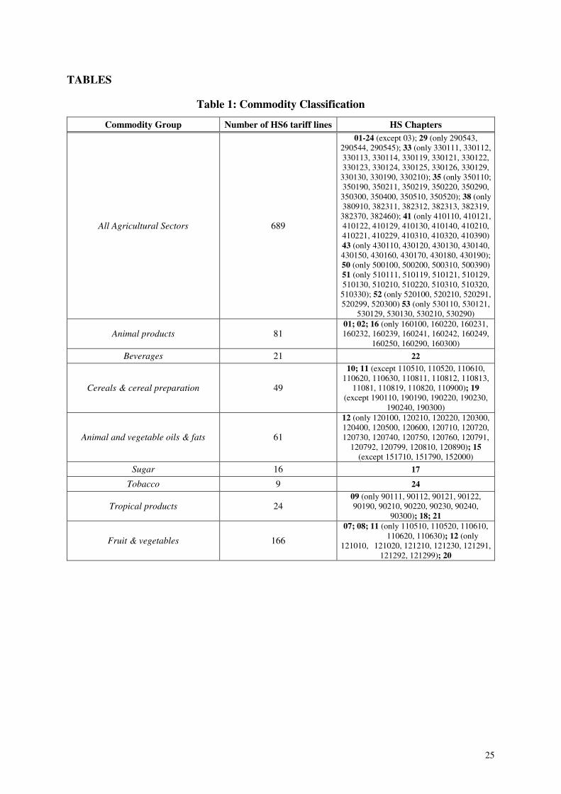
With regard to product detail, we define 8 groups (Table 1), according to WTO
Multilateral Trade Negotiations (MTN) Categories and the product concordance to HS Code
Commodity Classification provided by the World Integrated Trade Solution (WITS), 9 and
estimate separate regressions for each group. Developing countries agricultural exports cover
quite a wide range of goods (87% with respect to the total number of possible products, i.e. 7 When we consider the EU as a whole, the distance variable is computed as an average distance while the language and colonial links dummies are equal to 1 if they are different from zero for at least one EU member. 8 Martin and Pham (2008) show that Heckman estimators perform better than other estimators and overcome the “zero flows” problem only if true identifying restrictions are available. 9 We do not include the commodity groups that never present significant results in our regressions. These groups – chemicals, flowers, dairy, skins, feeding stuff for animals, and miscellaneous products – account for almost 25% of total agricultural imports.

15
689) with a weight equal to 60% of total EU agricultural imports. Figure 1 shows the share of
EU agricultural imports by type of tariff regime. Almost half of agricultural imports refers to
the MFN duty-free tariff lines although this percentage is much lower for animal products,
sugar, vegetables and cereals. If we consider the products facing a positive MFN duty, a
significant share of imports (30%) benefits from a positive preference margin. On the other
hand, some differences emerge when we look at the commodity groups: the share of
preferential imports ranges from 8% for animal products to almost 76% (where 64% is
preferential duty-free) for sugar.
Table 2 shows the percentage of tariff lines associated with positive trade subject to MFN
or preferential duties: in both cases, we distinguish between duty-free and positive tariffs. In
order to have an idea of the utilization rate, we also compute the percentage of tariff lines
where some preferential imports are actually registered. More than 60% of tariff lines with
positive trade may (potentially) benefit from a preferential treatment but preferences are only
actually exploited in half of the cases.
If we look at the number of preferential tariff lines actually used, the shares are always
much lower especially for animal products. The vast literature on preferences utilization (see
section 2) points out the possible reasons such as the excessive administrative burden or
prohibitive sanitary and phyto-sanitary regulations. If we compare the percentages of Table 2
with those of Figure 1, MFN duty-free lines appear to represent one third of all agricultural
tariff lines and account for almost half of total imports. This is mostly due to the oils and fats
and tropical sectors since in almost all other sectors the share of MFN duty-free imports is
much lower. On the other hand, for cereals and animal products most imports pay the MFN
duties. More generally, we notice that the share of preferential trade (Figure 1) is significantly
lower than the share of preferential tariff lines, and this is true even if we limit the comparison
to the actually used preferences.
Looking at the simple average applied duties and preferential margins (Table 3), animal
products, cereals and sugar are characterized by the largest values in both cases. Since these
sectors represent only tiny shares of EU imports from DCs (Figure 2), the preferential policies
do not seem to compensate for higher MFN duties.
On the other hand, vegetables, tropical products, oils and fats account for the largest share
of imports, and indeed they face the lowest average applied tariff (Table 3) whereas tobacco,
as well as beverages, accounts only for 3% of total agricultural imports even if it faces a low
average tariff (8%), and benefits (on average) from modest preferential margins (22%).

16
5. Econometric results
We estimate Eq. (21) by adopting the Heckman two-step procedure to tackle the “zero
flows” problem. First, we compare the estimates obtained using agricultural imports into each
of the 15 European members (Table 4) with those generated considering total imports to the
EU15 (Table 5) in order to highlight how results can be sensitive to geographical aggregation.
Then, working with country data, we estimate the trade impact of preferential margin by
commodity groups (Table 6).
In each table we highlight the rows referring to the estimates regarding the impact of
preferential margins: in the first stage, this is the impact on the probability of registering a
positive trade flow whereas in the second stage it can be interpreted as an elasticity that
measures the responsiveness of trade intensity to the extent of the margins themselves.
Accordingly, the former may be considered an estimate of the impact on the extensive
margin, i.e., the share of positive agricultural trade flows originating from DCs over the total
number of positive agricultural trade flows registered by the EU whereas the latter provides
an estimate of the impact on the intensive margins, i.e., the shares of agricultural imports from
developing countries on total EU agricultural imports.
Table 4 presents the results for the overall regression using disaggregated data for 15
European members. Econometric results confirm that preferential access leads to a significant
expansion of trade between EU and developing countries both in terms of the extensive as
well as intensive margin. The probit coefficient implies that preferences increase the
probability of registering positive trade flows by 4%. The impact on trade intensity is large
and highly significant. The dummy coefficient suggests that preferential trade flows are more
than two times larger (exp(0.81) > 2.25) whereas the coefficient associated with the
preference margin is equal to 1.29. Accordingly, a 10 per cent points increase of the EU
preference margins may lead to an increase of EU agricultural imports of 12.9 per cent.
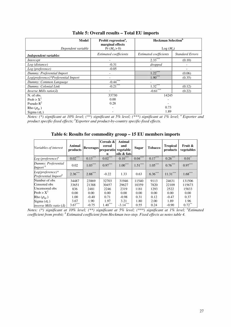
Looking at the results obtained using aggregated EU imports (Table 5), the first stage
coefficient for the probability of trading is not significantly different from zero. On the other
hand, both trade intensity coefficients are significant and higher than in the previous case.
Accordingly, geographical aggregation may lead to an underestimation of the impact on the
extensive margin and implies an overestimation of the impact on trade intensity.
In both regressions the coefficient of the preference dummy is positive, highly significant,
and much larger than the explicit preference intensity measure. Apparently, in addition to the

17
obvious benefits of the price margins granted by the preference schemes, these schemes
provide other more subtle, and in some cases even larger, benefits that accrue along the value
chain. These additional benefits may include greater access to (and lower cost) credit to cover
harvest expenses and other costs, and new business opportunities. The combination of the
competitive advantage and increased access to credit may contribute to greater economic
stability since farmers receiving preferential market access should be able to plan their
production better as well as personal, family and community needs.
The coefficient for the preference dummy variable has a point estimate of around 1.22 for
the aggregated EU. Such a result is broadly consistent with those provided by the literature
assessing the impact of different preference schemes mentioned in Section 2 (Haveman and
Schatz, 2003; Gaulier et al., 2004; Nilsson, 2005; Ảlvarez-Coque and Martì-Selva, 2006;
Amurgo-Pacheco, 2006; Verdeja, 2006; Pusterla, 2007; Agostino et al., 2007). However, the
comparison with the existing literature is not quite appropriate since usual econometric results
refer to aggregated data and cannot capture the variability of preference margins among
countries and products.
As far as the results for different commodity groups are concerned, some interesting
insights about the consequences of preferential policies on the extensive margin are provided
in Table 6. In all cases, preferences significantly increase the probability of exporting into the
EU markets. Such a probability of registering positive trade flows increases as a consequence
of the preference schemes varies between 1% for fruit and vegetables and 26% for tropical
products. Apparently, sectors characterized by higher shares of preferential duty-free tariff
lines tend to present a less diversified export structure (namely cereals, sugar, and animal
products).
The coefficients for the preference dummy variables have a point estimate ranging
between 0.76 and 1.51 (insignificant only for animal products) implying that the increase in
trade due to the implementation of preferences ranges between 4.5 (e1.51=4.5) for sugar and
2.1 (e0.76=2.1)for tropical products.
Looking at the intensive margins, it could be argued that a sector such as tropical products
characterized by the lowest (average) preference margin and the largest estimated coefficient,
should be considered the most promising from the developing countries point of view if they
were to ask for larger margins. However, such reasoning may be misleading. Tropical
products face the lowest applied tariffs and most imports (87%) enter the EU MFN duty-free.
In point of fact, the large impact of the EU preferences is due to a few tariff lines such as

18
“cocoa containing added sugar or other sweetening matter” that are highly protected. The
bottom line is that DCs have little to gain from an enlargement of the preference margins in
sectors such as tropical products and beverages where they already face (very) low applied
duties although they may have a lot to lose from preference erosion given the high sensitivity
of preferential trade flows.
Other sectors characterized by a large preferential trade elasticity are tobacco and fruit and
vegetables. In these cases, Figure 1 shows that there is some room for increasing the
preference margins both on MFN and preferential imports affected by positive duties.
However, tobacco only represents a tiny share of overall imports while the opposite is true for
fruit and vegetables (Figure 2).
Finally, it is worth mentioning animal products where most of imports are still subject to
positive, and still quite high (Table 3), MFN duties (Figure 1). Given the value of the
estimated coefficient (2.36), this is certainly the most promising sector for negotiating more
generous preferences.
6. Conclusions
Over time a number of preferential schemes have been granted by the EU to developing
countries in order to integrate them in world trade and promote their economic growth. In this
paper we focus on the agricultural sector since developing countries provide a significant
share of EU agricultural imports. The purpose of this work is to assess the impact of
preferential margins on trade flows using a gravity equation approach in order to single out
the contribution of the preferential policy to the deviation from “normal” trade levels.
We depart from the existing literature in two main respects. First, we work on highly
disaggregated trade data that quantifies the intensity of the preference margins rather than
relying on a simple dummy. In order to put the emphasis on the advantages granted with
respect to other competitors, preferential margins are computed for each product as the
difference between the highest tariff applied by EU and the actual duty paid by each exporter.
Secondly, we compare the results obtained by working at different level of geographic
aggregation and show how the choice of the importing region can also bias the final results.
Geographical aggregation produces an estimation bias since it pretends that there is only one
trade barrier for all countries in the same area while trade barriers may vary a lot across
importing countries (languages, colonial links, distances, and so on). Indeed, our results show

19
that the use of total EU imports leads to an underestimation of the impact of preferences on
the extensive margin whereas the impact on the intensive margin is largely overestimated.
From a methodological point of view, the main message is that there is little support for
the use of aggregated data either in terms of sectors, importing countries or preferential
policies. However, working at the most detailed level allowed by the data makes the problem
of zero trade flows quite serious. According to the most recent evidence provided by the
literature, we deal with this problem using the Heckman correction approach and control the
selection bias due to the presence of zeros.
Our results show that preferential schemes do have a significant impact on trade. First of
all, preferences influence the extensive margin of trade since we register a significant increase
in the probability of registering positive trade flows. This implies that countries benefiting
from a preferential scheme export a larger set of goods and some recent works have pointed
out the contribution of export variety to growth. Such an impact ranges from 1% for fruit and
vegetables and 26% for tropical products.
As far as the intensive margin is concerned, we find that import demand is quite elastic
with respect to the value of the preference margin. However, we also show that in addition to
the obvious benefits in terms of lower (or zero) duties, EU preferential schemes provide less
visible benefits that make the preferential trade flows more than double what they would
otherwise have been.
Finally, looking at the results for different commodity groups, our results have some
interesting policy implications. DCs should be afraid of the consequences of preference
erosion in sectors such as tropical products and beverages, characterized by large trade
elasticities. On the other hand, negotiation efforts to increase the preference margins should
be focused on sectors such as fruits and vegetables or animal products where most of imports
are still subject to positive and still quite high (Table 3) MFN duties.

20
References
Acosta Rojas G.E., Calfat G.G., Flores Jr R.G. (2005), Trade and Infrastructure: Evidences From the Andean Community, UNU-CRIS Occasional Papers N. O-2005/5.
Adam A., Kosma T. S., McHugh J. (2003), Trade-Liberalization Strategies: What Could Southeastern Europe Learn from the CEFTA and BFTA?, IMF Working Paper, WP/03/239.
Agostino M.R., Aiello F., Cardamone P. (2007), Analysing the Impact of Trade Preferences in Gravity Models. Does Aggregation Matter?, University of Calabria, TradeAG Working Paper 07/4.
Alexandraki K., Lankes H. P. (2004), The Impact of Preference Erosion on Middle-Income Developing Countries, IMF Working Paper 04/169, International Monetary Fund, Washington DC.
Alvarez-Coque J. M., Marti Selva (2006), A gravity approach to asses the effects of Association Agreements on Euromediterranean Trade of Fruits and Vegetables, Tradeag WP
2006/15.
Amurgo-Pacheco A. (2006), Preferential Trade Liberalization and the Range of Exported Products: The Case of the Euro-Mediterranean FTA. HEI Working Paper No. 18/2006, Graduate Institute of International Studies, Geneva.
Anderson J. E. (1979), A Theoretical Foundation for the Gravity Equation, American
Economic Review 69(1): 106-116.
Anderson J.E., van Wincoop E. (2003), Gravity With Gravitas: A Solution to the Border Puzzle, American Economic Review 93(1): 170-192.
Anderson J.E., van Wincoop E. (2004), Trade Costs, NBER Working Paper No. 10480.
Anson J., Cadot O., Estevadeordal A.,de Melo J., Suwa-Eisenmann A., Tumurchudur B. (2005), Rules of Origin in North–South Preferential Trading Arrangements with an Application to NAFTA, Review of International Economics 13(3): 501–517.
Augier P., Gasiorek M., Lai-Tong, C. (2005), The Impact of Rules of Origin in Trade Flows, In The Origin of Goods: Rules of Origin in Regional Trade Agreements edited by Cadot O., Estevadeordal A., Suwa A. and Verdier, T. CEPR/IADB/Oxford University Press, chap. 14.
Baier S. L., Bergstrand J. H. (2001), The Growth of World Trade: Tariffs, Transport Costs and Income Similarity, Journal of International Economics 53: 1-27.
Baldwin R.E. (1994), Towards an Integrated Europe, London: Centre for Economic Policy Research.
Bergstrand J. H. (1985), The gravity equation in international trade: some microeconomic foundation and empirical evidence, Review of Economics and Statistics 67: 474– 481.

21
Bergstrand J. H. (1989), The Generalized Gravity Equation, Monopolistic Competition, and the Factor Proportions Theory in International Trade, Review of Economic and Statistics 71: 143-53.
Bouët A., Jean S., Fontagné L. (2005), Is erosion of preferences a serious concern?, in Agricultural Trade Reform and the Doha Development Agenda, edited by K. Anderson and W. Martin, Washington, D.C.: The World Bank.
Brenton P. (2003), Integrating the Least Developed Countries into the World Trading System: The Current Impact of EU Preferences under Everything But Arms, Journal of World
Trade 37(3): 623-46.
Broda, Christian and David Weinstein (2006) Globalization and the Gains from Variety, Quarterly Journal of Economics 121(2): 541-85.
Bureau J.- C., Bernard F., Gallezot J., Gozlan E. (2004), The Measurement of Protection
on the Value Added of Processed Food Products in the EU, the US, Japan and South Africa. A Preliminary Assessment of its Impact on Exports of African Products, The World Bank, Final Report, July 26.
Candau F., Jean S. (2005), What Are EU Trade Preferences Worth for Sub-Saharan Africa and Other Developing Countries?, TradeAG Working Paper 05/09.
Cardamone P. (2007), A survey of the assessments of the effectiveness of Preferential Trade Agreements using gravity models, University of Calabria, TradeAG Working Paper.
Carrère C. (2004), African Regional Agreements: Impact on Trade with or without Currency Unions, Journal of African Economies 13(2): 199–239
Carrère C. (2006), Revisiting the Effects of Regional Trading Agreements on Trade Flows with Proper Specification of the Gravity Model, European Economic Review, Vol. 50.
De Maria F., Drogue S., Matthews A. (2008), Agro-Food Preferences in the EU’s GSP Scheme: An Analysis of Changes between 2004 and 2006, TradeAG Working Paper.
Eaton J., Kortum S. (2002), Technology, Geography and Trade, Econometrica 70(5): 1741-1779.
Eichengreen, B., Irwin, D. (1996). The Role of History in Bilateral Trade Flows. NBER Working Paper No. 5565.
Engel C. (2002), Comment on Anderson and van Wincoop in Brookings Trade Forum 2001, Susan Collins and Dani Rodrik, eds., Washington: The Brookings Institution.
Estevadeordal A, SuominenK. (2005), Rules of Origin: a World Map and Trade Effects, In The Origin of Goods: Rules of Origin in Regional Trade Agreements edited by Cadot O., Estevadeordal A., Suwa A. and Verdier, T. CEPR/IADB/Oxford University Press, chap. 4.
Feenstra R. C. (1994), New Product Varieties and the Measurement of International Prices, American Economic Review 84(1): 157-177.

22
Feenstra R. C. (1998), Integration of Trade and Disintegration of Production in the Global Economy, Journal of Economic Perspectives 12: 31-50.
Feenstra R. C. (2002), The Gravity Equation in International Economics: Theory and Evidence, Scottish Journal of Political Economy 49(5): 491-506.
Feenstra R. C., Kee H. L. (2004a), On the Measurement of Product Variety in Trade, American Economic Review 94(2): 145-149.
Feenstra R. C., Kee H. L. (2004b), Export Variety and Country Productivity, NBER Working Paper.
Feenstra R. C., Markusen J. (1996), Accounting for Growth with New Inputs, International Economic Review 35(2): 429-447.
Feenstra R. C., Yang T.-H., Hamilton G. G. (1999), Business Groups and Product Variety in Trade: Evidence from South Korea, Taiwan, and Japan, Journal of International
Economics 48(1): 71-100.
Funke M., Ruhwedel R. (2001a), Product Variety and Economic Growth: Empirical Evidence from the OECD Countries. IMF Staff Papers 48(2): 225–42.
Funke M., Ruhwedel R. (2001b), Export variety and export performance: empirical evidence from East Asia, Journal of Asian Economics 12: 493-505.
Gallezot J. (2005), Data Base on EU Preferential Trade TRADEPREF, TradeAG Working Paper 05/08.
Gallezot J., Bureau J.C. (2004), The utilisation of trade preferences by OECD countries: the case of agricultural and food products entering the European Union and United States, OECD, Paris.
Gaulier G., Jean S., Ünal-Kesenci D. (2004), Regionalism and the Regionalisation of International Trade, CEPII Working Paper No 2004-16.
Ghosh S., Yamarik S. (2004), Are regional trading arrangements trade creating? An application of extreme bounds analysis, Journal of International Economics 63: 369-395.
Haveman J.D., Schatz H. J. (2003), Developed Country Trade Barriers and the Least Developed Countries: The Economic Result of Freeing Trade, Working Paper No. 2003/7, Public Policy Institute of California
Head K., Mayer T. (2000), Non-Europe: The Magnitude and Causes of Market Fragmentation in the EU, Weltwirtschaftliches Archiv 136(2): 284-314.
Head K., Ries J. (2001), Increasing Returns versus National Product Differentiation as an Explanation for the Pattern of U.S.-Canada Trade, American Economic Review 91(4): 858-876.
Heckman J. (1979), Sample Selection Bias as a Specification Error, Econometrica 47(1): 153-161.

23
Helpman E., Melitz M., Rubinstein Y. (2007), Estimating trade flows: Trading Partners and Trading Volumes, NBER Working Paper No. 12927.
Hummels D. (1999), Have International Transportation Costs Declined?, Working Paper, Purdue University.
Hummels D. (2001), Toward a Geography of Trade Costs, Working Paper, Purdue University.
Linders G.-J. M., de Groot H. L. F. (2006), Estimation of the Gravity Equation in the Presence of Zero Flows, Tinbergen Institute Discussion Paper, TI 2006-072/3.
Manchin M. (2005), Preference Utilisation and Tariff Reduction in EU Imports from Africa, Caribbean, and Pacific Countries, World Bank Policy Research Working Paper, 3688.
Martin W., Pham C. (2008), Estimating the Gravity Model When Zero Trade Flows Are Frequent, mimeo, The World Bank.
Mold A. (2004), Trade Preference and Africa – The State of Play and the Issue at State, mimeo, The African Trade Policy Centre of the Economic Commission for Africa, United Nation, Economic Commission for Africa.
Nielsen C. P. (2003), Regional and Preferential Trade Agreements: a Literature Review and Identification of Future Steps. Report no. 155, Fodevareokonomisk Institut, Copenhagen.
Nilsson L. (2002), Trading relations: is the roadmap from Lomé to Cotonou correct? Applied Economics 34: 439-452.
Nilsson L. (2005), Comparative effects of EU and US trade policies on developing country exports, European Commission, TRADE Directorate General, Working Paper.
Oguledo V.I., MacPhee C.R. (1994), Gravity Models: a reformulation and an application to discriminatory trade arrangements, Applied Economics 26: 107-120.
Persson M. (2007), Trade Facilitation and the EU-ACP Economic Partnership Agreements: Who Has the Most to Gain?, mimeo, Lund University.
Persson M., Wilhelmsson F. (2005), Revisiting the Effects of EU Trade Preferences, Working Paper, Lund University, Sweden
Pusterla F. (2007) Regional Integration Agreements: impact, Geography and Efficiency. IDB-SOE Working Paper, January 2007.
Redding S., Venables A. J. (2000), Economic Geography and International Inequality, Centre for Economic Policy Research Discussion Paper No. 2568.
Rose A. K. (2004a) Do We Really Know that the WTO Increases Trade? American
Economic Review 94: 98-114.
Rose A. K. (2004b) Does the WTO Make Trade More Stable?, NBER Working Paper No. 10207.

24
Rose A. K., van Wincoop E. (2001), National money as a barrier to trade: The real case for monetary union, American Economic Review 91(2): 386–390.
Santos Silva J. M. C., Tenreyro S. (2005), The Log of Gravity, CEPR Discussion Paper No.5311.
Siliverstovs B., Schumacher D. (2007), Estimating gravity model: To log or not to log, Discussion Papers 739, German Institute for Economic Research, DIW Berlin.
Stevens C., Kennan J. (2004), Comparative Study of G8 Preferential Access Schemes for Africa, Report on a DFID Commissioned Study. Institute of Development Studies, University of Sussex.
Subramanian A., Wei S.J. (2005) The WTO promotes trade, strongly but unevenly. CEPR Discussion Paper No 5122.
Verdeja L. (2006) EU’s Preferential Trade Agreements With Developing Countries Revisited. Unpublished, University of Nottingham, School of Economics.
Wooldridge J. M. (2002), Econometric Analysis of Cross-Section and Panel Data, Cambridge, MA: MIT Press.
Yeyati L. E. (2003), On the impact of a common currency on bilateral trade, Economics
Letters 79(1): 125–129.
25
TABLES
Table 1: Commodity Classification
Commodity Group Number of HS6 tariff lines HS Chapters
All Agricultural Sectors 689
01-24 (except 03); 29 (only 290543, 290544, 290545); 33 (only 330111, 330112, 330113, 330114, 330119, 330121, 330122, 330123, 330124, 330125, 330126, 330129,
330130, 330190, 330210); 35 (only 350110; 350190, 350211, 350219, 350220, 350290, 350300, 350400, 350510, 350520); 38 (only 380910, 382311, 382312, 382313, 382319, 382370, 382460); 41 (only 410110, 410121, 410122, 410129, 410130, 410140, 410210, 410221, 410229, 410310, 410320, 410390) 43 (only 430110, 430120, 430130, 430140, 430150, 430160, 430170, 430180, 430190); 50 (only 500100, 500200, 500310, 500390) 51 (only 510111, 510119, 510121, 510129, 510130, 510210, 510220, 510310, 510320, 510330); 52 (only 520100, 520210, 520291, 520299, 520300) 53 (only 530110, 530121,
530129, 530130, 530210, 530290)
Animal products 81 01; 02; 16 (only 160100, 160220, 160231, 160232, 160239, 160241, 160242, 160249,
160250, 160290, 160300)
Beverages 21 22
Cereals & cereal preparation 49
10; 11 (except 110510, 110520, 110610, 110620, 110630, 110811, 110812, 110813,
11081, 110819, 110820, 110900); 19 (except 190110, 190190, 190220, 190230,
190240, 190300)
Animal and vegetable oils & fats 61
12 (only 120100, 120210, 120220, 120300, 120400, 120500, 120600, 120710, 120720, 120730, 120740, 120750, 120760, 120791,
120792, 120799, 120810, 120890); 15 (except 151710, 151790, 152000)
Sugar 16 17
Tobacco 9 24
Tropical products 24 09 (only 90111, 90112, 90121, 90122, 90190, 90210, 90220, 90230, 90240,
90300); 18; 21
Fruit & vegetables 166
07; 08; 11 (only 110510, 110520, 110610, 110620, 110630); 12 (only
121010, 121020, 121210, 121230, 121291, 121292, 121299); 20

26
Table 2: Share of EU agricultural tariff lines by type of tariff regime (2004)
% of Preferential duty-free tariff lines
% of Preferential duty tariff lines
Sample of positive trade
% of MFN duty-free tariff lines
% of MFN duty tariff lines
(no preference) Potential (Used) Potential (Used)
All Agricultural Sectors 30% 5% 25% (17%) 40% (17%) Animal products 6% 7% 26% (8%) 61% (15%) Beverages 43% 5% 24% (10%) 29% (17%) Cereals & cereal preparation 1% 6% 24% (11%) 68% (26%) Animal and vegetable oils & fats 38% 6% 32% (14%) 24% (12%) Sugar 1% 13% 18% (8%) 69% (28%) Tobacco 3% 4% 58% (27%) 35% (18%) Tropical products 29% 3% 45% (21%) 23% (6%) Fruit & vegetables 13% 4% 36% (18%) 46% (32%)
Table 3: Preference margins for commodity groups (2004)
Tariffs (simple averages) %
15 EU members
N. of Obs
Bilateral applied tariff Preference margin
Total Imports (Ml US$)
All Agricultural Sectors 477375 (36564)*
13 16 40,600
Animal products 34,487 32 34 2,307
Beverages 23,869 5 7 1,322
Cereals & cereal preparation 32,703 35 34 1,208
Animal and vegetable oils & fats 31,946 7 6 6,424
Sugar 11,540 70 40 1,309
Tobacco 9,113 8 22 1,206
Tropical products 24,631 2 5 5,583
Fruit & vegetables 144,010 8 11 11,100 * for aggregated EU15.
Table 4: Overall results – 15 EU members imports
Model
Dependent variable
Probit regressiona, marginal effects
Pr (Mij > 0)
Heckman Selectionb
Log (Mij)
Independent variables Estimated coefficients Estimated coefficients Standard Errors
Intercept - 20.80*** (0.82) Log (distance) -0.04*** -3.03*** (0.10) Log (preference) 0.04*** - Dummy: Preferential Import - 0.81*** (0.03) Log(preference)*Preferential Import - 1.29** (0.19) Dummy: Common Language 0.05*** - Dummy: Colonial Link 0.01*** 1.85*** (0.05)
Inverse Mills ratio(λ) - 2.40*** (0.07) N. of obs. Prob > Χ2
Pseudo R2
Rho (ρεµ ) Sigma (σε )
440934 0.00 0.59
- -
50391 - -
0.88 1.41
Notes: (*) significant at 10% level; (**) significant at 5% level; (***) significant at 1% level; aImporter,
Exporter and product specific-fixed effects; bImporter, Exporter and product-by-country specific-fixed effects.
27
Table 5: Overall results – Total EU imports
Model
Dependent variable
Probit regressiona, marginal effects
Pr (Mij > 0)
Heckman Selectionb
Log (Mij)
Independent variables Estimated coefficients Estimated coefficients Standard Errors
Intercept - 2.33*** (0.10) Log (distance) -0.31 dropped - Log (preference) -0.05 - - Dummy: Preferential Import - 1.22*** (0.06) Log(preference)*Preferential Import - 1.90*** (0.35) Dummy: Common Language -0.44*** - Dummy: Colonial Link -0.21*** 1.32*** (0.12) Inverse Mills ratio(λ) - -0.61*** (0.22) N. of obs. Prob > Χ2
Pseudo R2
Rho (ρεµ ) Sigma (σε )
33730 0.00 0.28
- -
14245 - -
0.73 1.89
Notes: (*) significant at 10% level; (**) significant at 5% level; (***) significant at 1% level; a
Exporter and
product specific-fixed effects; bExporter and product-by-country specific-fixed effects.
Table 6: Results for commodity group – 15 EU members imports
Variables of interest Animal
products Beverages
Cereals & cereal
preparation
Animal and
vegetable oils & fats
Sugar Tobacco Tropical products
Fruit & vegetables
Log (preference)a 0.02*** 0.13*** 0.02*** 0.10*** 0.04*** 0.17*** 0.26*** 0.01*
Dummy: Preferential
Import b 0.02 1.03*** 0.97*** 1.00*** 1.51*** 1.05*** 0.76*** 0.97***
Log(preference)*
Preferential Importb 2.36*** 2.88*** -0.22 1.33 0.63 6.36*** 11.31*** 1.68***
Number of obs Censored obs Uncensored obs Prob > Χ2
Rho (ρεµ ) Sigma (σε ) inverse Mills ratio (λ)
34487 33651
836 0.00 1.00 3.67
3.67***
23869 21388 2481 0.00 -0.40 1.90 -0.75
32703 30457 2246 0.00 0.71 1.97
1.40***
31946 29627 2319 0.00 -0.98 3.21
-3.14***
11540 10359 1181 0.00 0.31 1.80 0.55
9113 7820 1293 0.00 0.12 2.00 0.24
24631 22109 2522 0.00 -0.47 1.89 -0.90
131506 115673 15833 0.00 0.37 1.96
0.72**
Notes: (*) significant at 10% level; (**) significant at 5% level; (***) significant at 1% level; aEstimated
coefficient from probit; b Estimated coefficient from Heckman two-step. Fixed effects as notes table 4.

28
FIGURES
Figure 1: Share of EU agricultural imports by type of tariff regime (2004)
0%
10%
20%
30%
40%
50%
60%
70%
80%
90%
100%
All Agricultural
Sector
Tropical
products
Animal and
vegetable oils &
fats
Beverages Tobacco Cereals & cereal
preparation
Fruit &
vegetables
Sugar Food & live
animals
MFN duty free MFN duty Preferential duty free Preferential duty
Figure 2: Compositions of EU agricultural imports from DCs (2004)
Food & live animals
6%
Fruit & vegetables
27%
Tropical products
14%
Cereals & cereal preparation
3%
Animal and vegetable oils & fats
16%
Sugar
3%
Beverages
3%
Tobacco
3%
Others
25%