impact of eu agricultural policy on developing countries ... · impact of eu agricultural policy on...
TRANSCRIPT

Impact of EU agricultural policy on developing countries:A Uganda case study
Ole Boysen‡, Hans Grinsted Jensen§, Alan Matthews¶
July 2014
Abstract
Despite substantial reforms, the EU’s Common Agricultural Policy (CAP) is still
criticised for its detrimental effects on developing countries. This paper provides
updated evidence on the impact of the CAP on one developing country, Uganda. It
goes beyond estimating macro-level economic effects by analysing the impacts on
poverty. The policy simulation results show that eliminating EU agricultural support
would have marginal but nonetheless positive impacts on the Ugandan economy and
its poverty indicators. From the perspective of the EU’s commitment to policy co-
herence for development, this supports the view that further reducing EU agricultural
support would be positive for development.
Keywords: Uganda; Common Agricultural Policy; poverty; trade policy; domestic sup-port; computable general equilibrium-microsimulation
JEL classification: D58; F14; O10; O55
1 Introduction
The European Union’s (EU) Common Agricultural Policy (CAP) has long been criticisedfor its damaging effects on developing countries, and developing country agriculture inparticular. The CAP has provided extensive support to EU farmers, through both higherprices and budget support. The resulting stimulus to production, and disincentives toconsumption, meant that the EU emerged as a significant export competitor to developingcountry exporters, while its use of export subsidies enabled surpluses to be dumped at lowprices on the markets of importing developing countries. Case studies undertaken by non-governmental organisations (NGOs) have highlighted the alleged impact of EU exports
‡Ole Boysen, Agricultural and Food Policy, University of Hohenheim, Germany and Institute for Inter-national Integration Studies, Trinity College Dublin, Ireland, e-mail: [email protected].
§Hans Grinsted Jensen, Department of Food and Resource Economics, University of Copenhagen,Denmark, e-mail: [email protected].
¶Alan Matthews, Department of Economics and Institute for International Integration Studies, TrinityCollege Dublin, Ireland, e-mail: [email protected].
1

of particular commodities (milk powder, pig meat, poultry meat) in particular countries(APRODEV, 2007; Curtis, 2011; Fowler, 2002; Fritz, 2011; GermanWatch, 2008, 2009).At the same time, the EU’s high level of border protection for many CAP commoditieshas prevented low-cost developing country exporters from selling to the EU market exceptunder preferential access arrangements.
Model simulations confirm that the CAP has in the past distorted both the level andthe volatility of world market prices to the detriment of farmers in developing countries(Adenäuer & Kuiper, 2009; Costa, Osborne, Zhang, Boulanger, & Jomini, 2009; Gohin,2009; Gouel, Guillin, & P., 2008; Nowicki et al., 2009). However, the impacts on de-veloping countries are very diverse. By encouraging agricultural production in the EU,the CAP hurts those developing countries that are net food exporters and that would, oth-erwise, supply a larger share of the EU or world market. But the situation is less clearfor developing country exporters which have preferential access to the protected EU foodmarket or which are net food importers. Defenders of the CAP point to Europe’s open-ness to agricultural imports and underline that the EU is by far the largest importer ofagricultural products from developing countries (CEC, 2012). Consumers and net im-porting developing countries could have reaped some benefits from lower world marketprices (Panagariya, 2005); these countries, at least in the short run, are potential beneficia-ries of protected EU agricultural markets. Thus, there will be winners and losers amongdeveloping countries from the operation of the CAP (Matthews, 2008).
During the past twenty years, the CAP has undergone significant reform. The ‘newCAP’ is a rather different animal to the traditional policy widely, and rightly, criticised bydeveloping countries. According to OECD (2013), the Producer Support Estimate (PSE)for EU agriculture has fallen from 39% in 1986-88 to 19% in 2010-2012. More importantis that the share of trade-distorting support in the total has fallen from 98% to around 50%.This is reflected in the decline in the Nominal Protection Coefficient for EU agriculture,which has fallen from 1.72 in 1986-88 to 1.04 in 2010-2012. Nonetheless, it remainsthe case that EU farmers are still heavily subsidised, and for some products high tariffspersist. While reforms have been in a liberalising and market-oriented direction duringthe past two decades, a reversal of this trend cannot be excluded, particularly if currenthigh world market prices were to significantly collapse.
Policy coherence for development (PCD) means that the EU should take account ofthe objectives of development cooperation in all policies that it implements which arelikely to affect developing countries, and that these policies should support developmentobjectives where possible. The EU has adopted both a strong political and legal commit-ment to policy coherence for development (Carbone, 2008). Article 208 of the presentEU Treaty defines the overall objective of European development cooperation as follows:“The Union’s development cooperation policy shall have as its primary objective the re-
2

duction and, in the long term, the eradication of poverty. The Union shall take account
of the objectives of development cooperation in the policies that it implements which are
likely to affect developing countries.”
In the EU’s latest work programme on policy coherence, food security in develop-ing countries is one of five topics chosen for particular emphasis (Engel, Lein, Seters,& Helden, 2013). The European Commission in 2009 revised the guidelines for its exante impact assessment process for policy proposals under development to include PCD-relevant assessment indicators, noting the estimated impact of the proposed policy on thirdcountries in general, and particularly on its social, security and environmental impacts. Inaccordance with these guidelines, the impact assessment accompanying the Commission’slegislative proposals for the recent CAP reform included a discussion of the impacts of thereform on developing countries. The assessment noted that “impacts should be assessedon a case by case basis, as the economic, social, cultural and demographic heterogene-ity among and within developing countries, as well as the multitude of factors that affectfood security policies and situations in the short-, medium- and long-term, make gen-eralisations difficult. The assumption of direct price transmission mechanisms calls fora methodological approach that combines aggregate/national with household level data”(EC, 2011: 4).
This paper responds to this challenge by examining the impact of the CAP on Uganda.Uganda is one of the world’s least developed countries ($547 GDP per capita, currentUS$ in 2012) and has a high, if declining, share of its population living in poverty. It isthus representative of countries that are intended to be the focus of EU development aid.Uganda has a heavy dependence on agriculture. The sector employed 66% (2009) of thelabour force and accounted for 23% of total GDP in 2011.1 Agri-food exports accountedfor 64% of total exports in 2013.2 In 2013, 29% of Ugandan exports were destined for theEU of which 76% were agri-food products. Exports to the EU are highly concentrated ona few products: coffee, fish, other live plants, cocoa and tobacco account for 87% of totalexports to the EU. Most of Uganda’s main food staples (plantains, beans and cassava)are not widely traded, and the EU CAP does not significantly affect its main agriculturalexports nor does Uganda depend much on agri-food imports (11% of total imports). Im-ports from the EU consist mainly of chemicals and manufactures with a share of 5% ofagri-food products. As an LDC, and having initialled the interim EU–East African Com-munity (EAC) Economic Partnership Agreement (EPA), Uganda receives duty-free accessfor all of its exports to the EU. Moreover, its land-locked nature provides Uganda a certainamount of natural protection and thus limits the extent to which changes in world market
1Data retrieved from World Development Indicators, March 18, 2014, http://databank.worldbank.org.
2All trade-related data in this paragraph refers to the year 2013 and were retrieved from UN COM-TRADE via WITS, May 21, 2014, http://wits.worldbank.org.
3

prices are transmitted to domestic prices. Given these policy and structural characteris-tics, we do not expect the CAP to have major impacts, either positive or negative, on theUgandan economy. This, in itself, is a testable hypothesis. In addition, our methodologyillustrates the steps involved, and the data required, if one wishes to investigate the impactof the CAP on a developing country not only in aggregate terms but also in terms of itspoverty impacts.
Our objective in this paper is to examine the impact of EU agricultural policy by mod-elling the removal of trade and agricultural policy instruments supporting EU farmers andassessing the impact of the policy changes on prices and poverty in Uganda. We confinethe study to traditional agricultural support instruments (tariffs, export subsidies, directpayments) while recognising that agricultural trade can also be influenced by non-tariffbarriers such as health and safety standards, biofuel policies, environmental regulationsand climate regulation policies. A number of studies have simulated the impact on worldmarkets of eliminating CAP support instruments although, as we review below, these stud-ies are of limited usefulness in identifying the impacts of developing countries. The maincontributions of this study are to identify the specific impact of the CAP on Uganda (com-paring a scenario with and without the CAP) and to link the aggregate effect to Ugandanhousehold incomes and expenditure in order to estimate the impacts on poverty in thatcountry based on a computable general equilibrium (CGE) model framework.3
The simulations confirm that, on balance, further unilateral CAP reform would havepositive but very small overall effects on Uganda in terms of its GDP, poverty rates andfood security. Tracking the effect of this policy change through world and domestic pricechanges gives a better understanding of how changes in EU agricultural policy affecthouseholds in a developing country. We finally reflect on the usefulness of this approachto measuring the impact of EU non-aid policies on developing countries as part of PCD.
The paper is structured as follows. Following this motivation of the research question,Section 2 briefly reviews previous literature on the impact of the CAP on developingcountries. Section 3 briefly describes the two models and the databases used. Section 4describes the scenarios, how the models are linked to derive the poverty impacts of theCAP and the results of our simulations. Section 5 concludes.
3This study uses a consistent series of external shocks generated by a specific simulation of CAP reformin contrast to our earlier study which made use of synthetic shocks derived from the literature (Boysen &Matthews, 2012). We are also able to decompose the impact of CAP reform into the elimination of bordermeasures and the elimination of direct payments in this study.
4

2 Literature review and critique
There is an extensive literature on the ways in which the CAP impacts on developingcountries, but much of this is qualitative in nature and there are relatively few empiricalstudies. Empirical studies fall into two groups. On the one hand, case studies have beenundertaken, often by NGOs, examining the impact of EU exports of particular commodi-ties (milk powder, pig meat, tomato paste) in particular countries (see references above).A problem in interpreting these studies is that they do not develop a clear counterfactual ofwhat would happen in the absence of the CAP. Case studies generally start by examiningthe impact of EU trade flows (usually exports), although this is not the same as examiningthe impact of the CAP. Only if the EU would no longer export in the absence of the CAPmight it be justified to equate the impact of EU exports in a developing country with theimpact of the CAP. In some cases, the EU might indeed be a net exporter with the CAPbut a net importer in its absence. In other cases, the EU might still be an exporter with-out the CAP, even if a smaller one. Even if the EU were to cease exports, it is possiblethat the local market would be supplied by exports from another country rather than fromlocal production. Another criticism is that case studies usually focus on the impact ofEU exports in importing countries. But EU agricultural protection may also adverselyaffect the interests of developing country exporters, either directly by restricting accessto the EU market, or indirectly by competing with these exporters in third country mar-kets. Again, the main problem in identifying these effects on exporters is establishing thecounterfactual of what trade flows would occur in the absence of the CAP.
Modelling helps to address these two criticisms, but at the cost of introducing a newset of difficulties. In recent years, a wide array of simulation results has been published ex-amining the impact of agricultural protection in OECD countries on developing countries(Anderson & Martin, 2005; Anderson, Martin, & Van Der Mensbrugghe, 2006; Brooks,2014; McMillan, Zwane, & Ashraf, 2007; OECD, 2007). There is wide variation in thepublished empirical results. Partly, this variation reflects improvements that have takenplace in the models and databases over time. In part, the variation reflects the inherentcomplexities in modelling the causal links between EU policies (and OECD policies moregenerally) and their impacts in a developing country as well as the impact of the assump-tions that the modellers must make. However, relatively few studies publish the impactsof the CAP alone, simulated by a unilateral EU liberalisation of its agricultural policy. Ofthose published studies which do identify the impact of the CAP on world markets, manyare now considerably dated and are no longer a reliable guide to CAP impacts. Three ofthe more relevant studies are briefly reviewed.
The Scenar 2020-II study (Nowicki et al., 2009) contrasted a ‘Liberalisation’ scenariowith a ‘Reference’ scenario which carried forward the existing CAP orientation over the
5

period of the simulation. The ‘Reference’ scenario included a 20% reduction of the CAPbudget in real terms (constant in nominal terms), the implementation of the Single Pay-ment System (SPS) in all member states as of 2013, full decoupling, a 30% decrease indirect payments (DP) in nominal terms, a 105% increase of the European AgriculturalFund for Rural Development (EAFRD) and some trade liberalisation as a result of a DohaRound agreement. In the ‘Liberalisation’ scenario, all CAP trade-related measures arediscontinued. The CAP budget is reduced by 75% in real terms, all direct payments andmarket instruments are removed, and there is a similar increase in EAFRD expenditure asin the ‘Reference’ scenario.4 The ‘Liberalisation’ scenario also assumes full liberalisationof agricultural policy in other countries. This attenuates the effect of CAP liberalisationon EU agriculture, as does the limited amount of reform already foreseen in the ‘Ref-erence’ scenario. The modelling work employed a CGE model (LEITAP) and partialequilibrium models (ESIM, CAPRI). According to the Scenar-II study CAP liberalisa-tion would reduce the level of agricultural production in the EU with a greater impacton livestock products. The land and (to a lesser extent) segmented labour markets help tomaintain production as they absorb the negative impact of liberalisation due to a decline inland prices and a lower growth rate of agricultural wages. These two factors contribute tokeeping European agriculture competitive, along with the expected increase in productiv-ity. Only very aggregated results are reported for the impacts on third countries, but thereis a relatively higher growth in agricultural production in low-income countries (Centraland South America, Africa and Asia) in the ‘Liberalisation’ scenario.
Costa et al. (2009) is a GTAP5 application simulating the removal of all CAP instru-ments using version 7 of the GTAP database, which has a base year of 2004, althoughthe simulation is run for the year 2007. According to the modelling results, the CAPleads to higher output of the farm and food processing sectors in the EU, by about 8%and 6%, respectively, but lower output in the EU manufacturing and services sectors. Theadditional farm and food output in the EU is estimated to depress world prices for thesegoods by between 1% and 4%, while world prices for manufactured goods and servicesincrease. These price movements induce a contraction in agriculture and food processingin non-EU regions, and an expansion in the manufacturing and services sectors. In mostregions outside the EU welfare is lower because of the CAP, and would increase withCAP liberalisation (East Asia is an exception).
4The Scenar-II study also examines the implications of a third scenario, labelled the ‘ConservativeCAP’ scenario, in which Pillar 1 direct payments are increased relative to the ‘Reference’ scenario andPillar 2 payments significantly reduced (by 45%) to maintain the overall CAP budget constant.
5GTAP refers to the Global Trade Analysis Project which regularly updates and publishes the GTAPData Base, a fully documented, publicly available global data base which contains complete bilateral tradeinformation, transport and protection linkages, and which has also developed a standard GTAP model(T. W. Hertel, 1997), a multi-region, multi-sector, CGE model, with perfect competition and constant re-turns to scale, which is widely used to model trade liberalization scenarios.
6

Gohin (2009) uses a CGE model of the EU-15 to determine the effect of the CAP onworld prices. His model disaggregates the agri-food sector (32 primary agricultural com-modities, 30 food commodities and 10 animal feedstuffs, with the rest of manufacturingand services included as two further sectors). The model is calibrated to a 2005 socialaccounting matrix for the EU-15. The simulations are conducted against a baseline in2015 which takes account of the 2005 CAP Luxembourg reforms (decoupling of directpayments) but assumes no agreement on further WTO trade liberalisation. The simula-tion assumes the complete elimination of CAP and other agricultural policy instrumentsin 2015, including export subsidies, import tariffs, tariff rate quotas, the special safeguardmechanism, internal consumption subsidies, production quotas, direct payments and Pil-lar 2 payments. Direct payments are assumed partially coupled to production based ona literature survey of decoupling effects. Pillar 2 payments are modelled as direct sub-sidies to labour and capital. Gohin finds significant world market price effects from thissimulation of the elimination of the CAP, particular on world beef, maize and bioethanolmarkets. His estimates of the world market price changes resulting from elimination ofthe CAP are much greater than those in the other studies reviewed.
We conclude that there is a relatively thin recent empirical literature which examinesthe effect of the CAP on world markets, and the studies reviewed come to very differentresults regarding this impact. We therefore undertake an updated analysis using morerecent data and with a specific focus on identifying the impacts on Uganda.
3 Methodology
3.1 Model framework and database
3.1.1 Model framework
The model framework for the policy simulations consists of a sequence of two comparative-static CGE models. First, we use the GTAP model with version 8 of the database basedon 2007 data to simulate the CAP changes in the EU and its impacts on prices and tradebetween the different regions of the world. Then, the resulting changes in Ugandan tradeprices and quantities are passed to a detailed national model of Uganda as exogenous sim-ulation shocks. Their impacts on both the overall economy as well as households are thenassessed.
CAP-tailored GTAP model. The CAP reform in the EU and its world market impactsare simulated using a specially tailored CAP version of the multi-regional CGE modelGTAP. The standard GTAP model (Hertel 1997) is extended with policy variables and
7
equations making it possible to distinguish specific CAP budgetary payments, both na-tional or EU financed payments, within the model. Also the financing of the CAP ismodelled as a homogenous percentage contribution of national GDP by individual mem-ber states to the EU budget, whereby the model captures net transfers of payment betweenEU countries. Given these additional variables and equations the specially tailored CAPGTAP model is run on a database where each EU member country is specified individu-ally. The macroeconomic closure is neoclassical where investments are endogenous andadjust to accommodate any changes in savings. This approach is adopted at the globallevel, and investments are then allocated across regions so that all expected regional ratesof return change by the same percentage. Although global investments and savings mustbe equal, this does not apply at the regional level, where the trade balance is endoge-nously determined as the difference between regional savings and regional investments.The quantities of endowments (capital, land, labour, and natural resources) in each regionare fixed exogenously within the model. The Ugandan CPI is used as the numéraire forthe model.
Uganda model. For the detailed analysis of the Ugandan impacts, we adopt the single-country IFPRI Standard Computable General Equilibrium Model in GAMS (Löfgren,Harris, & Robinson, 2002). This choice is motivated by its excellent documentation andpublic availability which increase the transparency and ease of discussing the model andthe results. The reader is referred to the documentation in Löfgren et al. (2002) for an ex-haustive description and mathematical formulation of the model. Only model adaptationsand closure assumptions are presented here. To facilitate the microeconomic analysis ofincome distribution and poverty effects, the standard model is extended to incorporatethe full set of household observations from the nationally representative Uganda NationalHousehold Survey (UNHS) 2005/06 as individual households into the CGE model, alsocalled an “integrated CGE-microsimulation model”.6 Each household’s livelihood is char-acterized by its individual pattern of expenditures and income sources. But householdsare differentiated further. As in the IFPRI standard model, the consumption behaviourof households follows the Linear Expenditure System (LES) functional form. However,consumption preferences differ for each household as its LES is individually parame-terized by an own, idiosyncratic set of demand elasticities which is calculated from aneconometrically estimated flexible demand system (see Boysen, 2012). On the incomeside, each household differs by the quantities of the various factors it owns but also by theextent to which each of its labour types is utilized. Its labour utilization adapts to wage
6For a detailed discussion on various approaches for analysing household-level impacts on the basis ofCGE model extensions, see Bourguignon, da Silva, and Bussolo (2008), Boysen and Matthews (2008) orBussolo and Cockburn (2010).
8

changes within the extremes of unemployment and full employment. The potential foradditional labour supply (un- and underemployment) of individual households has beenderived from the UNHS data on unemployment, inactivity, and time-related underem-ployment of households’ members.7
In the standard model, commodities produced and sold on the domestic market areregarded as imperfect substitutes to imported commodities (“Armington assumption”).But as the CAP reform affects trade flows between Uganda and the EU differently thanthose between Uganda and other regions, it is important to further distinguish the externalaccount according to origin and destination of trade. Thus, the regions EU, East AfricanCommunity (EAC) and the rest of the world (ROW) are distinguished and imports fromthese regarded as imperfect substitutes. This is implemented in two levels. The higher-level Constant Elasticity of Substitution (CES) function aggregates imports from the EU,the EAC and the ROW together to a single imported commodity. The lower-level CESfunction combines imported and domestic goods into a final composite good which is soldon the domestic market. The elasticities of substitution between imports and domesticallyproduced goods have been adopted from T. Hertel, Hummels, Ivanic, and Keeney (2007).The elasticities of substitution between imports from different origins are twice the valueof the preceding ones.8 To facilitate the link to the results of the global CGE model, asexplained later, the constant elasticity of transformation (CET) export supply functionsof the standard model are replaced by downward-sloping export demand functions, sepa-rately for each export destination.9
The choice of “closures” has been guided by the goal to keep them as closely alignedwith those of the CAP GTAP model while introducing some country-specific detail intothe factor markets. However, these closures allow effects on household welfare whichcannot be measured in the model. This includes future welfare effects from saving, bor-rowing, and investment and non-monetary welfare provided through public goods andservices. Changes in government consumption cause unaccounted welfare effects throughchanged provision of public goods and services. Likewise, changes in government sav-ings imply unaccounted welfare effects in the future. In this model, the government reactsto changed revenue by adapting its spending on non-education, non-health services whilekeeping savings constant.10 The exchange rate adapts so that foreign savings remain con-
7Adopting the definition from the report on the UNHS (UBoS, 2006), time-related underemploymentrefers to individuals from the workforce which have worked less than 40 hours per week and are willingand able to provide more labour hours. For the present study, the actual number of additional labour hoursavailable is required.
8See T. Hertel et al. (2007) for a brief discussion of this “rule of two”.9Thereby giving up the small country assumption and the assumption that goods for the domestic and
export markets are differentiated.10The intention with this closure is to limit the effect of changes in government revenue on the provision
of public goods with a direct effect on the welfare of poor households.
9
stant. Investment is determined by total savings which depends on the fixed savings ratesof the households and the enterprise.
The way factor markets work has been modified compared to the standard IFPRImodel. Our analysis looks at a long term horizon. Accordingly, capital can depreciateand be reinvested in other sectors and is thus assumed to be fully mobile at a fixed supplylevel with rents clearing the market. Wage rates vary to clear the labour markets. But alsothe supplies of unskilled and skilled labour are assumed to increase with the associatedreal wage levels based on the so-called wage curve relationship introduced by Blanch-flower and Oswald (1995). They empirically found a relationship between the level of thereal wage and unemployment with an elasticity of unemployment with respect to the realwage level of approximately -0.1 valid across a large number of countries. Subsequently,this relationship and elasticity have been empirically confirmed by numerous studies forvarious countries, including the African countries Burkina Faso, Côte d’Ivoire, and SouthAfrica. Nijkamp and Poot (2005) subject the findings of the wage curve literature toa meta-analysis, confirm the stability of the negative real wage to unemployment rela-tionship, and suggest a publication-bias corrected elasticity of -0.07. Here, an elasticityof -0.1 is adopted. While the wage curve is observed on a macro level and thus is im-plemented to affect the aggregate supplies of skilled and unskilled labour, respectively,individual households might be limited in their potential to increase (fully employed) ordecrease (unemployed) their labour supply. Accordingly, the labour supply of each house-hold is modelled as being restricted from below by the state of unemployment and fromabove by full employment. More specifically, the labour utilization rate adapts in termsof percentage point changes uniformly for all households but some households are unaf-fected if their individual labour utilization rates are already at a limit. UBoS (2006, Table4.13) reports a time-related underemployment rate of 12.1% and an unemployment rateof 1.9%.
Also the land market is assumed to clear through rent adjustments. As climate andsoil conditions vary strongly across Uganda, crops, trees, and pastures cannot be grownwith the same productivity in all areas. To reflect these differences in productivity whenreallocating land between different crop uses, an approach presented by Keeney and Her-tel (2009) is adopted. According to this, each land owner has a fixed area of land and rentsit out to different activities with the goal of maximizing returns from land subject to limi-tations on the transformation of land from one use to another. As this limits the mobilityof land, rents differ between sectors. Here, the model formulation consists of a two-levelCET function nesting structure. On level one, the land owner decides on renting to annualor permanent crops or pastures. On the second level, the owner decides on renting to aparticular use within each group. The transformation of land use between the annual andpermanent crop and pasture groups as well as within the permanent group is assumed to
10

be rather sluggish with an elasticity of transformation of -0.25. By contrast, switchingland between uses for different annual crops is easier and an elasticity of transformationof -1.1 is assumed and a quasi-perfect elasticity of transformation between pastures fordifferent livestock types of -20.
The CPI is fixed and serves as the numéraire for the model.
3.1.2 Data
GTAP database. The simulations of global impacts of the EU CAP reform employ amodified version of the standard GTAP version 8 database (Narayanan, Aguiar, & Mc-Dougall, 2012).
The GTAP database is a system of multi-sector economy-wide input/output tables(countries) linked at the sector level through trade flows between commodities used bothfor final consumption and intermediate use in production. The database version 8 em-ployed in this analysis represents the global economy in the year 2007 and divides theglobal economy into 112 countries/regions where the present EU 27 member states arespecified as individual countries. The database specifies 57 commodities where 12 are pri-mary and 8 are secondary agricultural commodities. In this analysis, the GTAP databaseis aggregated to 28 regions with 25 EU member countries/regions specified together withUganda, rest of EAC and the rest of the world (ROW).11 On the commodity side, thedatabase is aggregated in a way to best match the commodity representation used for thenational Uganda model resulting in 32 commodities where the 12 primary agriculturalplus the forestry and fishing commodities are maintained.12
The modifications to the standard GTAP database identify the CAP agricultural do-mestic support payments by country and sector and enable direct modelling of the corre-sponding policy changes. Specifically, the agricultural domestic support payments foundin the standard GTAP database originate from the OECD’s Producer Support Estimate(PSE) tables. These correspond to the EU’s Pillar 1 decoupled payments to farmers andare reported by the EU as Green Box payments under the WTO Agreement on Agricul-ture. A condition for Green Box payments is that they should have no or minimal impacton trade. The literature, however, has brought forward evidence that the EU’s direct pay-ments are not fully decoupled from production but there is little evidence on the degree ofsuch coupling (Urban, Jensen, & Brockmeier, 2014). This study adopts the assumptionthat direct payments are coupled to output to some degree and thus bias the productionpattern. To modify the standard GTAP database, the PSE table for the EU year 2007 has
11The results for the individual 25 EU member countries/regions are aggregated to EU 27 results withinthe CAP-specific GTAP model providing results for the EU 27 which are transmitted to the Uganda model.
12The 8 secondary agricultural commodities are aggregated to 5, the 20 manufacturing commodities to7 and the 15 services commodities to 6 commodities.
11

been disaggregated so that domestic support payments are allocated to individual membercountries and calibrated into the model as input, output, and land-, capital-, labour-basedsubsidies (for details, see Urban et al., 2014).
In the CAP-tailored GTAP database used in our simulations, the standard calibrationof the direct payments single farm payment into the GTAP database is maintained as itoccurs in the standard GTAP database. This implies that the direct payments are allocatedin the database as a generic homogenous input subsidy rate to land, labour and capital em-ployed in the primary agricultural sectors. Given the initial distribution of factor incomesin the primary agricultural sectors found in the data, this means that roughly 85% of thedirect payments removed in the CAP liberalization scenario are, to some degree, coupledto production. The remaining 15% are decoupled from production representing the aver-age share of land rents found in the EU 27 countries. Given this calibration, the effects onUganda resulting from our simulations of cuts of the EU direct payments are among thestrongest effects we can suspect to happen if the CAP is liberalised. The calibration ofthe GTAP database could, however, be altered to reflect a lower degree of coupling (seeUrban et al., 2014, for a discussion on the subject).
Details of the CAP protection by sector in the CAP-tailored GTAP 8 (2007) databaseare shown in Table 1. In 2007, the EU had two digit tariffs on processed meat, rice and
Table 1: EU border and direct payment support for primary and processed agricultural prod-ucts, per cent
Direct payments
Import tariff Export subsidy Land Labour Capital
Paddy rice 9 0 10 10 10Wheat 6 0 14 15 15Other cereal grains 3 0 13 14 14Vegetables, fruit, nuts 6 1 13 13 13Oil seeds 0 0 13 14 13Sugar cane, sugar beet 0 0 14 14 14Plant-based fibers 0 0 16 17 17Other crops 1 0 13 13 13Bovine cattle, sheep and goats, horses 3 3 18 17 14Other animal products 2 0 14 14 14Raw milk 0 0 15 15 15Wool, silk-worm cocoons 0 0 15 15 14Meat products 17 5 0 0 0Processed rice 24 0 0 0 0Sugar 75 98 0 0 0Other food products 6 0 0 0 0Beverages and tobacco products 6 0 0 0 0
Source: Own computations from the CAP-tailored GTAP 8 database. Direct payment subsidies aspercentages of the respective factor input value.
sugar while processed sugar was the main receiver of export subsidies. Export refundsamounted to 1.4 billion euro in 2007 with 509 million euro spent on sugar and 513 million
12

euro on milk products (included in the meat sector). Direct aid in the EU amounted to37 billion euro in 2007 with roughly 32 billion euro being accounted for by the singlefarm payment (SFP) and single area payment scheme (SAPS). The remainder of roughly5 billion euro of direct aid mainly represents the remaining coupled payments still foundin France, Spain and Greece in 2007. Henceforth, the term ‘direct payments’ is used tocomprise the named three types. Table 1 shows that this is equivalent to an input subsidyrate of between 10% to 17% when aggregated up to EU averages by sector. The CAPreform scenario reduces these input subsidy rates to zero removing roughly 32 billioneuro of support together with the 5 billion euro of other direct support still remaining inFrance, Spain and Greece (not shown in Table 1). In addition, all primary and processedagricultural import tariffs and export subsidies are reduced to zero.
Data for the Uganda model. The detailed national Uganda model builds on the datafrom the 2007 social accounting matrix (SAM) for Uganda constructed by Thurlow (2008)which is extended to include the complete set of households from the UNHS 2005/06. 13
The final, extended Uganda SAM comprises 21 agricultural and 29 non-agricultural sec-tors, unskilled and skilled labour, land, and capital as factors of production, as well asaccounts for an enterprise, the government, household transfers, the rest of the world, andfinally 7,421 households. The SAM data (based on the national accounts) and the house-hold data (drawn from the household survey) are reconciled by a series of procedures.14
The structure of the final SAM is summarized in Table 2. Additionally, import values andtariffs from the TRAINS database (UNCTAD, 2010) are used for disaggregating Ugan-dan imports and exports (see Table 3) by origin as well as for construction of the tariffscenarios.
3.2 Poverty lines and measures
For measuring poverty, we employ an absolute poverty line and the measures Pα in-troduced by Foster, Greer, and Thorbecke (1984). The measure is defined as Pα =
1N
·N∑i=1
(z−yiz
)α · Ii with N : population size, z: poverty line, yi: income of individual
i, and Ii = 0 if yi < z and Ii = 1 otherwise. Setting the parameter α to 0, 1, or 2 com-putes the poverty headcount, gap, or severity index, respectively. The poverty headcountindex P0 measures the percentage of people falling below the poverty line. The povertygap P1 measures what percentage of the poverty line the average poor person needs asadditional income to reach the poverty line.
13Although a newer household survey is available for Uganda, the UNHS 2005/06 has been adopted asit also was the basis to construct the 2007 Uganda SAM.
14A technical appendix describing the reconciliation is available from the authors on request.
13

Table 2: The structure of Uganda’s domestic industry and trade in 2007, per cent
Share intotal pro-duction
value
Share intotal
valueadded
Share intotal
exports
Exportshare in
output ofthe sector
Share intotal
imports
Importshare indemand
for com-modity
Importtariff
Share intotal
importtariff
revenue
Share intotal
house-hold
homecon-
sumption
Share intotal
house-hold
marketcon-
sumption
Maize 1.2 1.7 1.9 18.6 0.8 13.3 0.1 0.0 2.4 0.2Rice 0.3 0.4 – – – – – – – –Other cereals 1.0 1.4 1.7 22.8 1.9 33.8 0.3 0.0 2.7 0.4Cassava 1.7 2.4 – – – – – – 10.2 1.3Irish potatoes 0.4 0.3 – – – – – – 1.2 0.3Sweet potatoes 1.9 2.5 – – – – – – 12.3 0.8Beans 2.2 2.6 4.3 27.1 – – – – 7.3 1.8Vegetables 0.6 0.9 0.0 0.5 – – – – 2.6 2.0Matooke 2.6 4.0 – – – – – – 15.7 2.4Fruits 0.7 1.0 0.1 4.2 0.1 4.4 7.9 0.0 3.8 0.9Oil seed crops 0.7 0.9 0.2 3.3 0.1 4.5 0.1 0.0 1.8 1.0Cotton 0.1 0.1 1.1 100.0 – – – – – –Tobacco 0.4 0.5 3.5 96.5 – – – – – –Coffee 0.8 0.8 7.4 100.0 – – – – – –Tea leaves 0.2 0.3 2.3 100.0 – – – – – –Other export crops 0.2 0.2 1.5 63.0 – – – – – –Cattle 1.3 1.6 – – – – – – – –Poultry 0.4 0.3 0.0 1.8 0.0 1.9 3.8 0.0 1.9 0.4Other livestock 0.2 0.3 0.2 11.3 – – – – 0.1 0.4
Total primary agriculture 16.8 22.2 24.2 16.4 2.9 5.2 0.4 0.1 62.1 12.0Fish 1.4 2.1 5.4 37.0 – – – – 0.2 1.3Forestry 1.8 2.1 1.6 8.5 – – – – 1.2 4.1
Grain milling 1.9 0.6 – – 1.1 8.6 8.6 0.6 3.9 4.1Meat processing 1.4 0.1 0.7 4.1 0.8 7.1 0.4 0.0 3.4 5.1Fish processing 0.7 0.1 5.7 58.3 0.5 13.3 2.0 0.1 0.0 0.9Other food processing 2.9 0.9 8.1 23.8 4.0 18.5 6.9 1.8 0.6 6.4Animal feed processing 0.3 0.1 – – – – – – – –Beverages & tobacco 1.1 0.5 0.5 3.5 1.0 10.5 9.7 0.6 0.6 3.3
Total food processing 8.4 2.3 15.0 14.5 7.4 12.2 6.5 3.0 8.6 19.8Manufacturing 6.3 4.0 9.5 11.5 66.6 45.9 22.9 96.9 0.1 18.2Services 65.4 67.3 44.4 7.0 23.0 6.3 0.0 0.0 27.9 44.7
Total 100.0 100.0 100.0 10.6 100.0 15.6 15.7 100.0 100.0 100.0
Source: Own computations from the extended 2007 Uganda SAM.
14

Table 3: Distribution of imports to and exports from Uganda by region and sector, per cent
Sector’s sharein total imports
Share in sector’simports
Sector’s sharein total exports
Share in sector’sexports
EAC ROW EU EAC ROW EU
Maize 0.79 2.6 15.1 82.3 1.87 96.3 0.0 3.7Other cereals 1.88 5.7 7.6 86.7 1.66 74.8 0.0 25.2Beans – – – – 4.30 57.9 12.3 29.9Vegetables – – – – 0.04 13.0 60.4 26.6Fruits 0.08 44.9 0.0 55.1 0.13 1.9 75.4 22.7Oil seed crops 0.14 50.9 6.0 43.1 0.16 15.9 21.4 62.6Cotton – – – – 1.09 13.1 0.0 86.9Tobacco – – – – 3.52 23.1 40.1 36.8Coffee – – – – 7.41 0.2 35.5 64.3Tea leaves – – – – 2.28 99.5 0.2 0.3Other export crops – – – – 1.51 0.5 44.9 54.5Poultry 0.03 37.4 33.9 28.7 0.04 71.1 28.5 0.5Other livestock – – – – 0.23 0.7 26.1 73.2Forestry – – – – 1.56 19.9 56.4 23.7Fish – – – – 5.43 0.5 89.2 10.4Grain milling 1.06 11.4 8.0 80.6 – – – –Meat processing 0.79 35.4 25.3 39.3 0.68 52.7 13.0 34.3Fish processing 0.55 6.1 12.2 81.7 5.67 1.7 36.5 61.8Other food processing 4.02 18.2 6.5 75.3 8.12 20.0 19.2 60.8Beverages & tobacco 1.00 75.3 7.6 17.1 0.49 18.0 0.9 81.1Manufacturing 66.64 20.4 24.2 55.4 9.46 20.6 17.4 62.0Services 23.04 – – – 44.36 – – –
Total or weighted average 100.00 20.4 22.2 57.4 100.0 23.9 29.8 46.3
Source: Own computation from the 2007 Uganda SAM. As no data is available on the regional distri-bution of services imports and exports, the corresponding averages exclude services.
Rural and urban poverty lines are derived such that they reproduce the poverty head-counts reported in the UNHS Report on the Socio-Economic Survey (UBoS, 2006, Table6.3.2 (a)) when applied to the adjusted household survey data. The UBoS poverty linesare based on the cost of basic needs approach, which accounts for the cost of meetingphysical calorie needs and allows for vital non-food expenditure, such as clothing andcooking fuels, valued using the average consumption basket of the poorest 50% of thepopulation (UBoS, 2006, Section 6.3). The rural and urban poverty lines account for thedifferences in prices and consumption baskets of the respective subpopulations. Per capitaconsumption is used as the welfare measure. To facilitate the poverty analysis from theCGE-MS results, household consumption is measured as the sum of the values of mar-ket consumption and home consumption of own produce, both valued at market prices,which then is deflated by the household-specific CPI. It should be noted that our povertyclassification is not directly comparable with the classification in the official report of theUBoS (2006) due to differences in data adjustments.
15

4 Simulation scenarios and results
4.1 Scenarios
The basic scenario (CAP) modelled in this paper is the elimination of CAP protectionto EU agriculture. This is measured as removing all import tariffs and export subsidieson agri-food products and all Pillar 1 direct payments to farmers in the model base yearwhich is 2007. Milk and sugar quotas are implicitly in place in the database, but arenot removed in the simulation, with the result that the impact of eliminating the CAP onthese markets may be over-estimated (high sugar and dairy tariffs and export subsidies areremoved which is expected to lower EU production of these products, but we do not allowfor an offsetting increase in production due to the removal of quotas). Pillar 2 paymentsto farmers are kept in place as these are not viewed as providing protection and incomesupport but rather as responding to market failures or providing regional assistance, suchas agri-environment payments or payments to farmers in areas of natural constraints.
The respective contributions of the two main sets of instruments of the CAP to the totaleffect of the CAP scenario are disentangled by first simulating these in isolation beforelooking at the full CAP reform scenario. The scenario Border eliminates only bordermeasures (import tariffs and export subsidies) and keeps total EU budgetary paymentsconstant. The scenario Direct Payments (DP) only abolishes the direct payment measures.
Uganda scenarios. As the 2007 Uganda SAM is based on 2003 supply and use tables,it does not well reflect the current import tariff structure which changed substantiallywhen Uganda formed the East African Community (EAC) customs union together withBurundi, Kenya, Rwanda, and Tanzania and correspondingly adopted the EAC’s com-mon external tariff (CET). To update Uganda’s tariff structure to the CET, a first scenario(2009) simulates the implementation of the EAC CET by adopting the tariff changes ob-served between 2003 and 2009 according to the UNCTAD TRAINS database (UNCTAD,2010). These results are not of interest by themselves for this study and thus are notshown but they serve as a synthetic baseline for the following simulations.15
The three scenarios for the simulations with the national Uganda CGE model are giventhrough the changes in import prices and export prices and quantities between Uganda andthe three regions EAC, ROW, and EU as determined by the results from the GTAP modelsimulations. To apply these results as external shocks to the Uganda CGE model, we adoptan approach suggested by Horridge and Zhai (2005). In order to align the trade behaviourof the single country model with that of the GTAP model, exports are determined bydownward-sloping export demand functions with elasticities corresponding to the import
15The more detailed results not reported in this paper are available from the authors on request.
16

substitution elasticities of the GTAP model.16 For the policy simulations, the locations ofthe export demand functions are shifted by changing the corresponding location parameterFP calculated from the GTAP simulation results for export prices and quantities togetherwith the elasticities.17 As for the import side, these authors argue that the consistencyis sufficiently established by applying the import price change for the respective countryfrom the global model results as import price changes to the single country model.
To illustrate the interpretation of the shocks to the location parameter assume a nega-tive percentage change in the location parameter of the demand function for exports fromUganda. This implies that the curve gets steeper (more L-shaped) and shifts towards theorigin. Thus, ceteris paribus, the export price and the quantity exported of this productdecrease.
4.2 Results
For each scenario, we first explain the global effects from the GTAP model which causethe specific trade price and quantity changes that are applied as exogenous shocks to thenational Uganda model and then continue with the Uganda model results. Note, onlyaggregate totals are shown for the non-food manufacturing and the services sectors, re-spectively, to reduce the size of the Uganda model-related tables. Moreover, economicvalues are given in real terms unless stated otherwise.
According to economic intuition, the removal of each of the three CAP policy mea-sures (import tariffs, export subsidies, and direct payments) leads to increasing worldmarket prices in the agri-food sectors affected. In addition, the reallocation of factors inthe EU towards more efficient sectors reduces prices in the non-food manufacturing andservices sectors as well as in the sectors which initially received less CAP support.
The effect on non-EU countries arises from both the direct changes in their trade withthe EU and the changes in their terms of trade as implied by the changes in world marketprices. The direction of the change in the terms of trade of each country depends on thecomposition of its import and export trade. In addition, if the EU cuts tariffs on importsfrom some particular country more than those from another country then the relative com-petitiveness of the latter country on the EU market and hence the quantity of imports fromthat country will be reduced. Such preference erosion concerns, in particular, developingcountries which already have quota- and duty-free access to the EU for their imports. TheEU can be expected to improve its welfare from the removal of distortions and result-
16Export demand functions are of the form QE =(
FPPWE
)ESUBMwith FP : location parameter, PWE :
the domestic price of exports and ESUBM : the GTAP Armington elasticity.17The shock for FP is calculated ∆FP = FP1
FP0=(
QE1
QE0
) 1ESUBM · PE1
PE0where QE 0,QE 1: the export
quantities and PE : the corresponding export prices from the results of the respective GTAP model scenariosimulations.
17
ing more efficient allocation of resources. For other countries, however, the direction ofwelfare effects is ambiguous ex ante.
4.2.1 Border scenario
Global results. The border scenario has two elements: the removal of the EU’s tariffson agri-food imports from, and the EU’s subsidies on agri-food exports to, non-EU coun-tries. Together, both elements lead to gains in the EU’s GDP of 0.04% in total. Loweringthe EU’s agri-food border protection drives down domestic food prices through cheaperimports and exports and stimulates domestic demand. With lower prices, EU agri-foodproduction decreases – while manufacturing and services expand – and EU demand in-creases resulting in excess demand on the ROW market and hence rising prices in theROW. This shortage also causes trade prices between the ROW and Uganda to rise. As inthe ROW resources are drawn into the agri-food sectors, factor costs and in consequencealso prices in the non agri-food sectors increase there. However, as imports to the EU fromdifferent origins are regarded as imperfect substitutes (due to the Armington assumption)and agri-food imports from Uganda are now relatively more expensive compared to thosefrom other countries for which import tariffs are now removed, the EU demand for agri-food imports from Uganda decreases (the EU demand curve for exports from Ugandashifts to the left). In general, EU export prices to Uganda tend to fall as a consequenceof lower EU domestic prices. This is counter-balanced in the meat processing and otherfood processing sectors (which includes sugar) where the removal of previously high EUexport subsidies means that Ugandan prices for EU imports increase for these products.Imports from the EAC to Uganda also become cheaper because the removal of EU importtariffs shifts trade from exporters with preferential trade arrangements, such as the EAC,to other exporters; thus EU demand for EAC agri-food products and, consequently, pricesdecrease as well. The resulting trade shock applied to the Uganda model is shown inTable 4.
Uganda results. The removal of EU agri-food tariffs has no direct impact on Ugan-dan trade which, in 2007, already had duty and quota free access to the EU market onbasis of the Cotonou Agreement and the Everything but Arms scheme.18 Nevertheless,Ugandan trade is affected indirectly because the EU’s import tariffs against third coun-tries are dropped. This leads to a loss of preferences vis-à-vis other exporters to the EU(preference erosion) and hence to a decrease in EU demand for Ugandan exports. Other
18The EU introduced the Everything but Arms scheme as a special arrangement under its GeneralisedSystem of Preferences in 2001. It provides duty-free and quota-free access to all least developed countriesfor all export commodities except arms. Duty-free access was delayed for bananas until January 2006, forsugar until July 2009 and for rice until September 2009 so trade barriers on these products from Ugandaremain in the GTAP database.
18

Table 4: Border scenario: percentage changes to Ugandan export demand function locationparameters and import prices
Export demandlocation parameter
Import price
Uganda model sector EAC ROW EU EAC ROW EU GTAP sectors mapped
Maize -0.07 0.76 -2.32 -0.10 0.67 -1.10 GrainsOther cereals -0.06 0.73 -2.23 -0.02 0.65 -1.12 Wheat; grainsBeans 0.10 0.76 -2.51 – – – Vegetables, fruit, nutsVegetables 0.10 0.76 -2.51 – – – Vegetables, fruit, nutsFruits 0.10 0.78 -2.53 -0.06 0.75 -1.13 Vegetables, fruit, nuts;
sugar cane, sugar beetOil seed crops -0.01 1.13 -1.76 -0.07 0.89 -1.31 Oil seedsCotton 0.33 0.50 0.27 – – – Plant-based fibersTobacco -0.08 0.56 -1.00 – – – Other cropsCoffee -0.08 0.56 -1.00 – – – Other cropsTea leaves -0.08 0.56 -1.00 – – – Other cropsOther export crops -0.08 0.56 -1.00 – – – Other cropsPoultry 0.22 0.64 -2.51 -0.09 0.75 -1.64 Animal products necOther livestock 0.22 0.64 -2.51 – – – Animal products necForestry 0.05 0.17 0.08 – – – ForestryFish -0.06 0.38 -1.49 – – – FishingGrain milling – – – 0.00 0.43 -0.52 Processed rice; other
food productsMeat processing 0.24 0.95 -3.26 0.00 0.65 1.16 Raw milk; meatFish processing 0.04 0.33 -1.69 0.01 0.40 -0.52 Other food productsOther food processing 0.05 0.51 -1.67 -0.02 0.53 0.56 Sugar; other food prod-
uctsBeverages & tobacco -0.04 0.12 -0.82 0.01 0.32 -0.32 Beverages and tobacco
productsTextiles & clothing 0.20 0.23 0.07 0.05 0.30 -0.08 Wool and silk; textiles,
apparel, leatherWood & paper products 0.10 0.18 -0.01 0.02 0.25 -0.01 Wood and paper prod-
uctsMining 0.19 0.17 0.19 0.15 0.17 0.15 MiningFuels – – – 0.16 0.18 0.13 Petroleum, coal productsChemicals & fertilizer 0.11 0.16 0.05 0.04 0.25 -0.05 Chemical, rubber, plastic
productsOther manufacturing 0.12 0.17 0.06 0.05 0.24 -0.03 Other manufacturingMachinery & equipment 0.12 0.18 0.07 0.06 0.24 -0.01 Machinery and equip-
mentFurniture 0.12 0.17 0.06 0.05 0.24 -0.03 Other manufacturingUtilities 0.06 0.17 0.01 – – – UtilitiesHotels & catering 0.02 0.19 -0.05 – – – TradeTransport services 0.09 0.18 0.09 0.04 0.25 -0.02 TransportCommunication services 0.02 0.15 -0.01 -0.01 0.26 -0.13 CommunicationFinancial & banking services 0.03 0.16 0.06 -0.02 0.26 -0.05 Banking and insuranceOther private services 0.07 0.16 -0.02 -0.00 0.27 -0.11 Other services
Source: Own computation from GTAP Border scenario results.
19

exporters faced tariffs of up to 9% for primary agricultural products and up to 75% forprocessed food. At the same time, the import tariff abolition reduces EU internal pricesfor these products increasing EU demand and correspondingly prices on the world mar-ket. The removal of EU export subsidies, in contrast, affects Ugandan imports from theEU (mainly the fruits, meat processing and other food processing sectors) directly byincreasing their prices.
The overall outcome is a matter of empirical analysis. Table 5 shows that the elimi-nation of CAP border measures will lead to a deterioration in Uganda’s terms of trade. Inquantity terms, imports decrease by 0.13% while exports increase by 0.05%. The detailedresults (not provided) show imports in all sectors but poultry declining. The picture on theexport side is mixed. Exports from the majority of agri-food sectors including fish declineby 6% or less with the most notable exceptions being oil seed crops, cotton and processedmeat exports which rise by 1% to 2% (see Table 6). Exports from the important manufac-turing and services sectors, amounting to 9% and 44% of total exports, rise by 1.3% and0.3%, respectively. GDP decreases marginally (-0.02%). Output increases marginally inaggregate and there is a slight shift in production towards those expanding export sectors.Private consumption decreases by 0.06% distributed across all sectors. The governmentreduces spending marginally to compensate for lower revenue. The real incomes of thepoor tend to decrease in similar magnitude for rural and urban households as shown inTable 7. This scenario causes an increase of 0.01 percentage point in the national povertyheadcount equivalent to 2,720 additional people falling into poverty. Equally, the povertygap increase by 0.01 points. Figure 1 illustrates that the overall effect of this scenario is aslight increase in the poverty headcount and gap irrespective of the choice of the povertyline.
4.2.2 Direct payments (DP) scenario
Global results. EU GDP increases by 0.02%. Within the EU, the reduction in directpayments (even if only partially coupled to production) increases production costs andraises prices of the agricultural sectors and their upstream processing industries. Thequantity demanded is lower at higher prices causing EU agri-food markets to rebalance ina new equilibrium with higher prices and lower quantities. This creates shortages and in-creases prices on world markets. Moreover, reduced agri-food production stimulates pro-duction in the non agri-food sectors where market prices tend to fall. Hence, EU demandfor imports increases in the agri-food and decreases in the non agri-food sectors; likewise,prices for exports from the EU tend to increase in the agri-food and to decrease in othersectors. In contrast to the border scenario, the DP scenario causes similar shocks to boththe EAC and the ROW. Both regions increase their demand for agricultural commodities
20

Table 5: Macroeconomic results
Base Border DP CAP
GDP components (real) % of GDP % change from Base
Private consumption 76.96 -0.06 0.20 0.15Investments 20.78 -0.06 0.26 0.21Government consumption 11.80 -0.01 0.02 0.00Total absorption 109.77 -0.06 0.19 0.14Exports 15.59 0.05 -0.40 -0.36Imports -25.37 -0.13 0.40 0.29GDP at market prices 100.00 -0.02 0.05 0.03Net indirect taxes 9.13 -0.12 0.37 0.26GDP at factor cost 91.09 -0.00 0.01 0.00
Government revenue Share in total % change from Base
ROW transfers 43.01 0.02 -0.06 -0.04Direct taxes 23.73 -0.08 0.16 0.09Import taxes 11.09 -0.26 0.25 -0.02Sales taxes 22.16 -0.02 0.05 0.03
Factor income distribution Share in total point change from Base share
Labor unskilled 38.62 -0.00 -0.02 -0.02Labor skilled 12.89 -0.00 -0.00 -0.01Land 8.53 0.01 0.06 0.07Capital 39.96 -0.00 -0.04 -0.05
Closure variables change from Base
Terms of trade (%) -0.03 0.06 0.03Real exchange rate (%) 0.04 -0.09 -0.05Nominal exchange rate (%,UGX/USD)
0.02 -0.06 -0.04
Government spending onadministration (%)
-0.01 0.03 0.01
Source: Own computation from CGE simulation results.
21

Table 6: Border scenario results: Percentage changes from Base
Quantity
Output Exports ImportsHousehold
consumptionConsumer
prices
Maize 0.03 0.03 -0.42 -0.07 0.03Rice -0.02 – – – –Other cereals 0.16 0.45 -0.36 -0.18 0.16Cassava -0.02 – – -0.02 -0.04Irish potatoes -0.02 – – -0.03 -0.04Sweet potatoes -0.02 – – -0.02 -0.05Beans 0.02 0.17 – -0.03 -0.03Vegetables -0.03 -4.38 – -0.02 -0.04Matooke -0.01 – – -0.02 -0.06Fruits -0.09 -5.94 -0.52 -0.03 -0.03Oil seed crops 0.06 2.08 -0.67 -0.04 -0.02Cotton 1.51 1.51 – – –Tobacco -0.40 -0.42 – – –Coffee 0.11 0.11 – – –Tea leaves -0.03 -0.03 – – –Other export crops -0.25 -0.40 – – –Cattle 0.08 – – – –Poultry -0.03 -1.27 0.35 -0.04 -0.04Other livestock -0.03 -0.25 – -0.02 -0.06
Total primary agriculture 0.01 0.04 -0.39 -0.03 -0.03Fish -1.32 -2.97 – -0.01 -0.07Forestry -0.00 0.56 – -0.08 0.00
Grain milling -0.02 – -0.39 -0.09 0.03Meat processing 0.09 1.03 -1.24 -0.08 0.01Fish processing -0.73 -1.33 -0.34 -0.06 0.00Other food processing 0.08 0.07 -0.51 -0.13 0.09Animal feed processing 0.02 – – – –Beverages & tobacco -0.02 0.26 -0.07 -0.06 -0.00
Total food processing -0.03 -0.43 -0.50 -0.09 0.03Manufacturing 0.35 1.29 -0.11 -0.15 0.06Services 0.01 0.30 -0.03 -0.03 -0.04
Total 0.01 0.05 -0.13 -0.08 0.00
Source: Own computation from CGE simulation results. Household consumption is valued at marketprices.
22

Table 7: FGT poverty indices and consumer price indices for the poor
Base Border DP CAP
NationalHeadcount 30.01 0.01 -0.09 -0.06Gap 8.85 0.01 -0.03 -0.02
RuralHeadcount 33.25 0.01 -0.09 -0.07Gap 9.84 0.01 -0.03 -0.02
UrbanHeadcount 12.68 0.02 -0.08 0.00Gap 3.57 0.01 -0.01 -0.01
Poor only-CPI 100.00 -0.01 0.11 0.11
Source: Own computation from CGE simulation results. The columns show point changes in theindices from the Base column. The poverty figures use rural and urban poverty lines, respectively.
from Uganda but decrease it for processed foods and manufacturing and services. Ugan-dan imports from these regions become more expensive in case of primary agriculturalproducts and cheaper for others. These results are reflected in the trade shock applied tothe Uganda model, see Table 8.
Uganda results. A large share of Ugandan imports is manufactured goods and a largeshare of its exports is agri-food products (neglecting services exports which are mainlytourism-related), so that the terms of trade improve by 0.06%. Correspondingly, produc-tion shifts towards exported agri-food products where output increases the most in thecash crop sectors (by 3% to 6% for tobacco, other export crops, tea and coffee, see Table9). The strong expansion in those agri-food sectors tends to increase consumer pricesfor other products through higher prices for primary factors and inputs. By contrast, theprice for manufactures drops by 0.3% and its output by 1.2%. Overall, output dropsby 0.03%. Uganda’s primary agriculture expands but food manufacturing declines; ex-ports become more concentrated on primary commodities and the import dependence fornon-food manufactures and services increases. In aggregate, exports decrease by 0.4%,imports increase by 0.4%, GDP at market prices increases by 0.05% and household andgovernment consumption as well as investments increase by 0.2%, 0.02% and 0.26%,respectively.
GDP at factor prices increases marginally (0.01%) and the factor income distributionshifts marginally from capital, and less from unskilled labour, to land (Table 5) allowingconsumption to increase. But for the average poor household, the CPI actually increasesbecause the prices for primary agricultural and food processing commodities increase.
23

Table 8: Direct payments scenario: percentage changes to Ugandan export demand functionlocation parameters and import prices
Export demandlocation parameter
Import price
Uganda model sector EAC ROW EU EAC ROW EU GTAP sectors mapped
Maize 0.68 0.26 5.28 0.54 -0.15 6.18 GrainsOther cereals 0.67 0.30 5.10 0.40 0.01 6.23 Wheat; grainsBeans 0.89 0.42 4.38 – – – Vegetables, fruit, nutsVegetables 0.89 0.42 4.38 – – – Vegetables, fruit, nutsFruits 0.89 0.42 4.35 0.27 0.03 8.28 Vegetables, fruit, nuts;
sugar cane, sugar beetOil seed crops 0.76 0.30 3.54 0.40 0.07 4.99 Oil seedsCotton 0.09 0.10 2.19 – – – Plant-based fibersTobacco 1.54 0.89 3.21 – – – Other cropsCoffee 1.54 0.89 3.21 – – – Other cropsTea leaves 1.54 0.89 3.21 – – – Other cropsOther export crops 1.54 0.89 3.21 – – – Other cropsPoultry 0.64 0.66 4.14 0.70 -0.08 2.83 Animal products necOther livestock 0.64 0.66 4.14 – – – Animal products necForestry -0.17 -0.73 -0.77 – – – ForestryFish -0.06 -0.62 -1.12 – – – FishingGrain milling – – – 0.03 -0.46 0.37 Processed rice; other
food productsMeat processing -0.02 -0.06 2.10 -0.02 -0.41 1.72 Raw milk; meatFish processing -0.01 -0.33 0.05 0.00 -0.50 0.36 Other food productsOther food processing -0.01 -0.35 0.06 0.09 -0.47 0.36 Sugar; other food prod-
uctsBeverages & tobacco -0.04 -0.39 -0.25 -0.08 -0.59 -0.06 Beverages and tobacco
productsTextiles & clothing -0.41 -0.62 -0.68 -0.16 -0.64 -0.83 Wool and silk; textiles,
apparel, leatherWood & paper products -0.47 -0.69 -0.85 -0.15 -0.70 -0.82 Wood and paper prod-
uctsMining -0.79 -0.76 -0.76 -0.72 -0.76 -0.77 MiningFuels – – – -0.70 -0.75 -0.79 Petroleum, coal productsChemicals & fertilizer -0.57 -0.71 -0.81 -0.20 -0.70 -0.85 Chemical, rubber, plastic
productsOther manufacturing -0.60 -0.72 -0.81 -0.29 -0.71 -0.87 Other manufacturingMachinery & equipment -0.71 -0.73 -0.80 -0.35 -0.71 -0.86 Machinery and equip-
mentFurniture -0.60 -0.72 -0.81 -0.29 -0.71 -0.87 Other manufacturingUtilities -0.50 -0.74 -0.84 – – – UtilitiesHotels & catering -0.37 -0.71 -0.75 – – – TradeTransport services -0.56 -0.75 -0.78 -0.23 -0.71 -0.87 TransportCommunication services -0.53 -0.76 -0.85 -0.07 -0.71 -0.93 CommunicationFinancial & banking services -0.41 -0.76 -0.83 0.03 -0.70 -0.96 Banking and insuranceOther private services -0.57 -0.75 -0.86 -0.01 -0.70 -0.94 Other services
Source: Own computation from GTAP Direct payments scenario results.
24
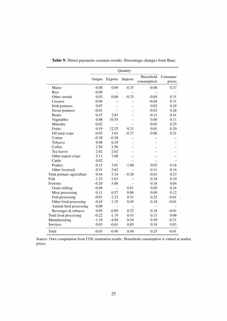
Table 9: Direct payments scenario results: Percentage changes from Base
Quantity
Output Exports ImportsHousehold
consumptionConsumer
prices
Maize 0.08 0.69 -0.35 -0.08 0.37Rice -0.09 – – – –Other cereals 0.03 0.68 -0.25 -0.04 0.31Cassava -0.04 – – -0.04 0.31Irish potatoes 0.07 – – 0.02 0.18Sweet potatoes -0.01 – – -0.03 0.26Beans 0.47 2.63 – -0.11 0.41Vegetables 0.08 10.55 – 0.06 0.11Matooke -0.02 – – -0.05 0.25Fruits 0.19 12.25 0.21 0.01 0.20Oil seed crops -0.03 3.63 -0.37 -0.06 0.31Cotton -0.38 -0.38 – – –Tobacco 6.08 6.29 – – –Coffee 2.56 2.56 – – –Tea leaves 2.62 2.62 – – –Other export crops 5.11 7.68 – – –Cattle 0.02 – – – –Poultry 0.15 3.81 -1.00 0.03 0.16Other livestock 0.51 3.62 – 0.11 0.14
Total primary agriculture 0.44 3.14 -0.28 -0.01 0.23Fish -1.33 -3.03 – 0.10 0.10Forestry -0.20 -3.66 – 0.18 0.04
Grain milling -0.09 – 0.81 0.05 0.16Meat processing 0.11 0.57 0.08 0.09 0.12Fish processing -0.81 -1.23 0.51 0.22 -0.01Other food processing -0.43 -1.35 0.45 0.18 -0.01Animal feed processing 0.09 – – – –Beverages & tobacco 0.05 -0.89 0.25 0.18 -0.01
Total food processing -0.22 -1.19 0.43 0.13 0.06Manufacturing -1.19 -4.94 0.54 0.59 -0.31Services 0.03 -0.61 0.05 0.18 0.03
Total -0.03 -0.40 0.40 0.25 -0.01
Source: Own computation from CGE simulation results. Household consumption is valued at marketprices.
25

−0.10
−0.05
0.00
0.05
−0.06
−0.04
−0.02
0.00
0.02
Headcount
Gap
50 100 150 200Percent of poverty line
Poi
nt d
iffer
ence
in in
dex
CAP Border DP
Figure 1: Sensitivity of FGT poverty indices to the choice of the poverty line
Nevertheless, the overall effect is a decrease in the poverty headcount by 0.09 pointsequivalent to a reduction of 24,480 poor people. The gap to the poverty line for theaverage poor person narrows by 0.03 points. In terms of the FGT poverty indices, the ruralpoor benefit slightly more than the urban. Considering a range of alternative poverty lines(Figure 1), the EU’s removal of direct payments tends to have a slight poverty alleviatingeffect, even when other poverty lines are considered.
4.2.3 CAP scenario
Global results. The CAP scenario combines the previous two policy changes, i.e., theremoval of border measures and of direct payments, simultaneously. This causes EU GDPto increase by 0.05%. The directions of change of demand for Ugandan exports and ofthe prices for imports from these regions to Uganda are ambiguous in cases where the two
26

policy changes work in opposite directions. In the simulation results, the EU increasesdemand for Ugandan agricultural and decreases that for other exports, see Table 10. Fromthe EU, agricultural commodities become more expensive in Uganda, processed foodprices tend to remain stable and other products become cheaper. The directions of effectson trade between Uganda and the ROW and the EAC are the same except for demand forUgandan processed foods which increases.
Uganda results. For Uganda, the total effect is an increase in the terms of trade of0.03% and a negligible increase in GDP of 0.03%. Exports decrease by 0.4% and im-ports increase by 0.3%. Total output decreases by 0.02% and there is a broad shift inproduction towards agricultural export sectors which expand by 3.3% on average (Table11). Other sectors largely shrink including manufacturing (-0.9%) and fish and processedfish (-2.7% and -1.6%). Household consumption increases by 0.2% due to the factor re-turns distribution shifting mainly from capital to land. How this affects individual poorhouseholds depends on the changes in the returns to the factors they own and their indi-vidual consumption preferences. The CPI specifically calculated for the population belowthe poverty line increases reflecting that prices for almost all agri-food products increase.The CAP abolition decreases the national poverty headcount by 0.06 points equivalent tolifting 16,320 out of poverty. The decrease in the poverty gap by 0.02 points indicates ageneral but minor income gain for people living below the poverty line. Figure 1 high-lights that the impact on the headcount varies quite strongly with different poverty linesbut both headcount and gap reduce irrespectively of the line chosen. Thus, CAP elimina-tion could have a slightly poverty alleviating effect in Uganda. Rural households turn outto benefit more than urban ones as the headcount remains unchanged for the latter.
5 Review and conclusions
The EU’s CAP has long been criticised for its incoherence with the EU’s developmentpolicy objectives, the primary and overarching objective of which is the eradication ofpoverty in the context of sustainable development (CEC, 2005). But, over time, the CAPhas been reformed slowly in a more market-oriented direction and developing countrieshave become more heterogeneous. This has led the European Commission to conclude:“With the mostly criticised negative effects largely addressed over the previous consec-utive reforms through a decoupling of payments and a gradual elimination of export re-funds, the implications of the current CAP reform for development are limited. The CAPhas become more market oriented, thereby considerably reducing its potential negativeimpacts on world markets. Therefore past criticisms about the negative effects on globalfood security are no longer relevant” (CEC, 2013, p. 106).
27

Table 10: CAP removal scenario: percentage changes to Ugandan export demand functionlocation parameters and import prices
Export functionlocation parameter
Import price
Uganda model sector EAC ROW EU EAC ROW EU GTAP sectors mapped
Maize 0.63 1.09 2.99 0.44 0.57 5.15 GrainsOther cereals 0.64 1.11 2.90 0.39 0.73 5.18 Wheat; grainsBeans 1.02 1.27 1.88 – – – Vegetables, fruit, nutsVegetables 1.02 1.27 1.88 – – – Vegetables, fruit, nutsFruits 1.02 1.28 1.83 0.20 0.85 7.54 Vegetables, fruit, nuts;
sugar cane, sugar beetOil seed crops 0.76 1.53 1.93 0.34 1.04 3.79 Oil seedsCotton 0.46 0.67 2.58 – – – Plant-based fibersTobacco 1.54 1.59 2.35 – – – Other cropsCoffee 1.54 1.59 2.35 – – – Other cropsTea leaves 1.54 1.59 2.35 – – – Other cropsOther export crops 1.54 1.59 2.35 – – – Other cropsPoultry 0.90 1.38 1.60 0.62 0.73 1.20 Animal products necOther livestock 0.90 1.38 1.60 – – – Animal products necForestry -0.11 -0.54 -0.72 – – – ForestryFish -0.13 -0.25 -2.68 – – – FishingGrain milling – – – 0.03 -0.02 -0.15 Processed rice; other
food productsMeat processing 0.23 0.90 -1.49 -0.03 0.27 2.96 Raw milk; meatFish processing 0.04 0.02 -1.69 0.01 -0.09 -0.16 Other food productsOther food processing 0.04 0.18 -1.67 0.06 0.07 0.93 Sugar; other food prod-
uctsBeverages & tobacco -0.10 -0.26 -1.10 -0.08 -0.28 -0.40 Beverages and tobacco
productsTextiles & clothing -0.21 -0.39 -0.64 -0.12 -0.34 -0.94 Wool and silk; textiles,
apparel, leatherWood & paper products -0.38 -0.51 -0.90 -0.14 -0.47 -0.87 Wood and paper prod-
uctsMining -0.63 -0.62 -0.59 -0.60 -0.61 -0.64 MiningFuels – – – -0.57 -0.59 -0.68 Petroleum, coal productsChemicals & fertilizer -0.46 -0.55 -0.80 -0.17 -0.47 -0.93 Chemical, rubber, plastic
productsOther manufacturing -0.48 -0.56 -0.78 -0.26 -0.49 -0.93 Other manufacturingMachinery & equipment -0.59 -0.55 -0.77 -0.31 -0.49 -0.90 Machinery and equip-
mentFurniture -0.48 -0.56 -0.78 -0.26 -0.49 -0.93 Other manufacturingUtilities -0.46 -0.58 -0.86 – – – UtilitiesHotels & catering -0.36 -0.51 -0.83 – – – TradeTransport services -0.48 -0.58 -0.72 -0.20 -0.48 -0.92 TransportCommunication services -0.52 -0.61 -0.90 -0.09 -0.46 -1.10 CommunicationFinancial & banking services -0.39 -0.60 -0.81 -0.00 -0.45 -1.05 Banking and insuranceOther private services -0.51 -0.58 -0.92 -0.02 -0.44 -1.09 Other services
Source: Own computation from GTAP CAP scenario results.
28

Table 11: CAP removal scenario results: Percentage changes from Base
Quantity
Output Exports ImportsHousehold
consumptionConsumer
prices
Maize 0.12 0.73 -0.86 -0.15 0.43Rice -0.12 – – – –Other cereals 0.21 1.17 -0.68 -0.24 0.50Cassava -0.06 – – -0.06 0.28Irish potatoes 0.05 – – -0.00 0.14Sweet potatoes -0.03 – – -0.05 0.22Beans 0.48 2.78 – -0.13 0.39Vegetables 0.05 5.64 – 0.04 0.07Matooke -0.03 – – -0.07 0.21Fruits 0.09 5.63 -0.34 -0.02 0.17Oil seed crops 0.03 5.89 -1.14 -0.10 0.30Cotton 1.28 1.28 – – –Tobacco 5.94 6.15 – – –Coffee 2.80 2.80 – – –Tea leaves 2.73 2.73 – – –Other export crops 5.09 7.62 – – –Cattle 0.08 – – – –Poultry 0.11 2.45 -0.75 -0.00 0.13Other livestock 0.48 3.39 – 0.09 0.09
Total primary agriculture 0.47 3.30 -0.75 -0.04 0.20Fish -2.71 -6.11 – 0.10 0.04Forestry -0.22 -3.19 – 0.11 0.05
Grain milling -0.12 – 0.43 -0.04 0.21Meat processing 0.18 0.88 -1.16 0.02 0.13Fish processing -1.57 -2.62 0.16 0.16 -0.00Other food processing -0.37 -1.33 -0.06 0.06 0.08Animal feed processing 0.10 – – – –Beverages & tobacco 0.03 -0.67 0.19 0.13 -0.01
Total food processing -0.26 -1.71 -0.07 0.05 0.10Manufacturing -0.86 -3.67 0.45 0.46 -0.25Services 0.03 -0.34 0.03 0.16 -0.01
Total -0.02 -0.36 0.29 0.18 -0.01
Source: Own computation from CGE simulation results. Household consumption is valued at basemarket prices and consumer prices are weighted by base quantities.
29

While we broadly agree with this assessment the CAP retains a number of protection-ist features which potentially can impact on third countries (Matthews, 2014). The impactof the CAP on developing countries is an empirical question; this impact will differ de-pending on the economic, trade and poverty characteristics of each country. In this paper,we investigate the impact of the CAP on Uganda. Uganda is an appropriate country foranalysis as a least developed country with a high dependence on agriculture and a highshare of agri-food exports in total exports. It also benefits from unrestricted access (sub-ject to rules of origin) to the EU market for agri-food products under preferential tradeagreements. While we do not expect to find large impacts from further reform of the CAP,the approach we have adopted facilitates the identification of the transmission channelsbetween CAP reform and its household and poverty impacts in Uganda.
Our empirical results in simulating the removal of remaining border protection and di-rect payments to EU farmers suggest, indeed, that the impact on Uganda will be marginalbut nonetheless positive. Its terms of trade, GDP and household consumption all improveslightly as do the poverty indicators. These results are driven largely by the assumptionthat direct payments in the EU are only partially decoupled and encourage a higher level ofagricultural production than in the absence of the CAP. Note that the database employedimplies a rather high degree of coupling of direct payments to production and thus thesimulated effects of the CAP elimination are at the high end of what can be expected. Theremoval of border measures turns out to have a smaller impact and partly in an offsettingdirection.
To derive these results we had to make a number of assumptions about the presumedbehaviour of firms, households and the government in Uganda which could, no doubt,be improved in further work. A challenge facing all research on the poverty impact oftrade reform (though mostly overlooked in the literature to date) is to keep separate thepoverty impact of the trade reform itself from the poverty impact of the measures thegovernment has to take to maintain equilibrium and the modelling choices for the savingsand investment and the foreign account balances. In the results of the full CAP elimina-tion, however, government spending and real investment increase while foreign savingsare constant. Thus, these indicate potentially positive welfare in addition to the povertyreduction.
Another limitation of our results is that we cannot take proper account of the imper-fect price transmission of price changes not just across the Uganda border (internationalto Uganda transmission) but, more importantly, within Uganda. The Armington structurein the Uganda CGE model determining the demand for imports does imply that changesin border prices are only imperfectly transmitted to domestic prices, but within Ugandawe assume that all households, independent of their location or whether urban or rural,experience the same price effects. In reality, factors and goods are susceptible to frictions
30

in relocating spatially (depending, e.g., on geography and infrastructure) and thus pricesas well as their changes differ across Uganda’s area as shown, e.g., in Boysen (2009).Together with the strength of price signals transmitted, the induced reactions and welfareimplications may vary widely between households in different locations. As a result, weover-estimate the likely reallocation of resources within Uganda in response to CAP re-form. Because greater mobility of factors and goods help a specific household to bettercope with an adverse price shock but restricts the extent to which it can benefit from a pos-itive price shock, the effect on the overall welfare and poverty results of this assumptionis ambiguous.
However, our study is important in demonstrating the range of channels whereby CAPreform can impact on developing countries like Uganda. The effects are felt not just in themarkets for agri-food commodities but also in the markets for manufactures and services.The distribution of factor incomes changes, away from labour and capital towards land.Food prices become relatively more expensive, benefiting surplus producers but hurtingpoor consumers. Moreover, preference erosion adds a negative effect to the overall con-sequences for developing countries. In the Ugandan case, it appears that the CAP as itexisted in the late 2000s had some minor impact in lowering consumption and increasingpoverty, but we stress that the magnitude of these effects was very small. Further changessince then (the rise in global food prices since 2007 which has further lowered the effec-tive protection given to EU farmers, and the additional conditionality attached to directpayments in the 2013 CAP reform and the continued reduction in their real value) makethis impact smaller still.
References
Adenäuer, M., & Kuiper, M. (2009). A typical application of SEAMLESS-IF at macro
level: A trade liberalization scenario applied to the EU (Report No. 43). SEAM-LESS Integrated Project, EU 6th Framework Programme.
Anderson, K., & Martin, W. (2005). Agricultural trade reform and the Doha DevelopmentAgenda. The World Economy, 28(9), 1301-1327.
Anderson, K., Martin, W., & Van Der Mensbrugghe, D. (2006). Distortions to worldtrade: Impacts on agricultural markets and farm incomes. Review of Agricultural
Economics, 28(2), 168-194.APRODEV. (2007). No more chicken, please. Brussels: Author.Blanchflower, D. G., & Oswald, A. J. (1995). The wage curve (Vol. 1). Cambridge, MA:
The MIT Press.Bourguignon, F., da Silva, L. A. P., & Bussolo, M. (Eds.). (2008). The impact of macroe-
conomic policies on poverty and income distribution : macro-micro evaluation
31

techniques and tools. Washington, DC: The World Bank and Palgrave MacMil-lan.
Boysen, O. (2009). Border price shocks, spatial price variation, and their impacts on
poverty in Uganda (IIIS Discussion Paper Series No. No. 306). Institute for Inter-national Integration Studies, Trinity College Dublin.
Boysen, O. (2012). A food demand system estimation for Uganda (IIIS Discussion PaperSeries No. No. 396). Institute for International Integration Studies, Trinity CollegeDublin.
Boysen, O., & Matthews, A. (2008). The impact of developed country agricultural trade
liberalization on poverty: A survey (Mimeo). Trinity College Dublin.Boysen, O., & Matthews, A. (2012). Impact of EU Common Agricultural Policy reform
on Uganda (Research Report). London: Overseas Development Institute (ODI).Brooks, J. (2014). Policy coherence and food security: The effects of OECD countries’
agricultural policies. Food Policy, 44, 88-94.Bussolo, M., & Cockburn, J. (Eds.). (2010). Macro-micro analytics - a guide to combining
computable general equilibrium and microsimulation modelling frameworks (Vol.3(1)).
Carbone, M. (2008). Mission impossible: the European Union and policy coherence fordevelopment. Journal of European Integration, 30(3), 323-342.
CEC. (2005). The European Consensus on Development: Joint Statement by the Council
and the Representatives of the Governments of the Member States Meeting within
the Council, the European Parliament and the Commission. Brussels: Commissionof the European Union.
CEC. (2012). International aspects of agricultural policy, background document for
the Advisory Group on International Aspects of Agriculture, updated 30 January
2012. Brussels: Commission of the European Communities, Directorate-Generalfor Agriculture and Rural Development.
CEC. (2013). EU 2013 report on policy coherence for development. Brussels: Commis-sion of the European Union.
Costa, C., Osborne, M., Zhang, X., Boulanger, P., & Jomini, P. (2009). Modelling the
effects of the EU Common Agricultural Policy (Staff Working Paper). Melbourne:Productivity Commission.
Curtis, M. (2011). Milking the poor - how EU subsidies hurt dairy producers in
Bangladesh. Copenhagen, Denmark: ActionAid.EC. (2011). The Common Agricultural Policy and development: Annex 12, impact as-
sessment, Common Agricultural Policy towards 2020 - SEC(2011) 1153 final/2.
Brussels: European Commission, Directorate-General Agriculture and Rural De-velopment.
32

Engel, P., Lein, B., Seters, J. v., & Helden, B. v. (2013). EU policy coherence for food se-
curity: Aligning parallel agendas (ECDPM Discussion Paper No. 153). Maastricht,The Netherlands: European Centre for Development Policy Management.
Foster, J., Greer, J., & Thorbecke, E. (1984). A class of decomposable poverty measures.Econometrica, 52(3), 761-66.
Fowler, P. (2002). Milking the CAP: How Europe’s dairy regime is devastating livelihoods
in the developing world (Briefing Paper No. 34). Oxfam.Fritz, T. (2011). Globalising hunger: Food security and the EU’s Common Agricultural
Policy (CAP). Berlin: Transnational Institute, FDCL-Verlag.GermanWatch. (2008). Devastating floods - man made. Bonn: GermanWatch e.V.GermanWatch. (2009). Consequences of the EU trade and agricultural policy for Zam-
bia’s dairy farmers. Bonn: GermanWatch e.V.Gohin, A. (2009). Quelles conséquences d’une suppression de la politique agricole com-
mune après 2013? Revue d’Economie Politique, 119(4), 633-651.Gouel, C., Guillin, A., & P., R. M. (2008). American and European agricultural market
access: A concern for the South? (La Lettre du CEPII No. 277). Paris, France:CEPII.
Hertel, T., Hummels, D., Ivanic, M., & Keeney, R. (2007). How confident can we beof CGE-based assessments of free trade agreements? Economic Modelling, 24(4),611-635.
Hertel, T. W. (1997). Global trade analysis: Modeling and applications. CambridgeUniversity Press.
Horridge, J., & Zhai, F. (2005). Shocking a single-country CGE model with exportprices and quantities from a global model. In T. Hertel & L. Winters (Eds.), Poverty
and the WTO: Impacts of the Doha Development Agenda (p. 94-103). PalgraveMacmillan.
Keeney, R., & Hertel, T. W. (2009). The indirect land use impacts of United States biofuelpolicies: The importance of acreage, yield, and bilateral trade responses. American
Journal of Agricultural Economics, 91(4), 895-909.Löfgren, H., Harris, R. L., & Robinson, S. (2002). A standard computable general
equilibrium (CGE) model in GAMS (Microcomputers in Policy Research No. 5).Washington, DC: International Food Policy Research Institute (IFPRI).
Matthews, A. (2008). The European Union’s Common Agricultural Policy and develop-ing countries: the struggle for coherence. European Integration, 30(3), 381-399.
Matthews, A. (2014). Research handbook on the Common Agricultural Policy. InM. Cardwell & J. McMahon (Eds.), (chap. The CAP and development). Chel-tenham, UK: Edward Elgar Publishing.
McMillan, M., Zwane, A., & Ashraf, N. (2007). Globalization and poverty. In (p. 183-
33

240). University of Chicago Press.Narayanan, B., Aguiar, A., & McDougall, R. (Eds.). (2012). Global trade, assistance, and
production: The GTAP 8 data base. Center for Global Trade Analysis, Purdue Uni-versity. (Available online at: http://www.gtap.agecon.purdue.edu/
databases/v8/v8_doco.asp)Nijkamp, P., & Poot, J. (2005). The last word on the wage curve? Journal of Economic
Surveys, 19(3), 421-450.Nowicki, P., Goba, V., Knierim, A., van Meijl, H., Banse, M., Delbaere, B., & Helming, J.
(2009). Scenar 2020-II – update of analysis of prospects in the Scenar 2020 study -
contract no. 30-ce-0200286/00-21. Brussels: European Commission, Directorate-General Agriculture and Rural Development.
OECD. (2007). Agricultural policy and trade reform: The impact on world commodity
markets. Paris: OECD Publishing.OECD. (2013). Agricultural policy monitoring and evaluation 2013: OECD countries
and emerging economies. Paris: OECD.Panagariya, A. (2005). Agricultural liberalisation and the least developed countries: six
fallacies. The World Economy, 28(9), 1277-1299.Thurlow, J. (2008). A 2007 social accounting matrix for Uganda (Report). Washington,
DC: International Food Policy Research Institute (IFPRI).UBoS. (2006). Uganda National Household Survey 2005/06 - report on the socio-
economic module. Entebbe, Uganda: Uganda Bureau of Statistics.UNCTAD. (2010). UNCTAD TRAINS database. United Nations Conference on Trade
and Development, Geneva, Switzerland. (Accessed online via WITS, World Bankon November 22, 2010)
Urban, K., Jensen, H. G., & Brockmeier, M. (2014). Extending the GTAP data base and
model to cover domestic support issues using the EU as example (GTAP TechnicalPapers No. 35). Center for Global Trade Analysis, Department of AgriculturalEconomics, Purdue University.
34