etm 607 application of monte carlo simulation: scheduling radar warning receivers (rwrs)
DESCRIPTION
ETM 607 Application of Monte Carlo Simulation: Scheduling Radar Warning Receivers (RWRs). Scott R. Schultz Mercer University. Problem Statement. Develop an RWR scheduler that minimizes the time to detect multiple threats across multiple frequency bands. RWR Scheduling Definitions. - PowerPoint PPT PresentationTRANSCRIPT
August 27, 2012 ETM 607 Slide 1
ETM 607Application of Monte Carlo
Simulation:Scheduling Radar Warning
Receivers (RWRs)
Scott R. Schultz Mercer University
August 27, 2012 ETM 607 Slide 2
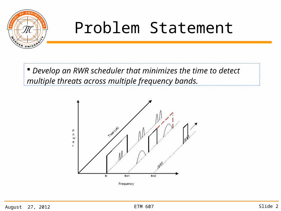
Problem Statement
Develop an RWR scheduler that minimizes the time to detect multiple threats across multiple frequency bands.

August 27, 2012 ETM 607 Slide 3
RWR Scheduling Definitions
Pulse Width (PW)
Revisit Time (RT)
IlluminationTime (IT)
Pulse RepetitionInterval (PRI)
Beam Width (BW)
Definitions:
Revisit Time (RT) – time to rotate 360 degrees (rotating radar)
Illumination Time (IT) – function of RT and BW
Pulse Width (PW) – length of time while target is energized
Pulse Repetition Interval (PRI) – time between pulses
Time
August 27, 2012 ETM 607 Slide 4
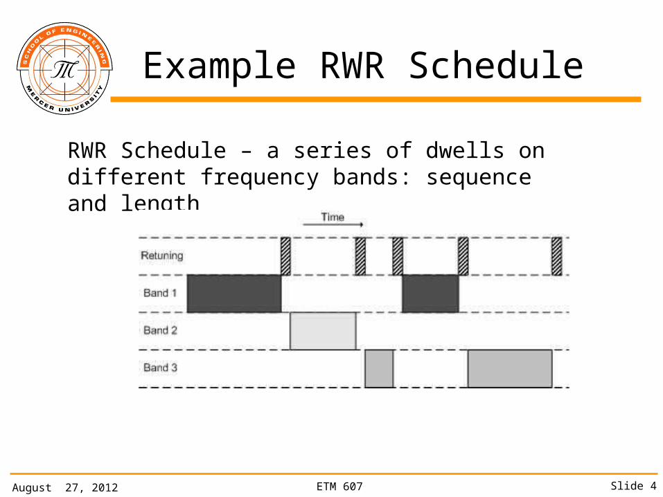
Example RWR Schedule
RWR Schedule – a series of dwells on different frequency bands: sequence and length
August 27, 2012 ETM 607 Slide 5
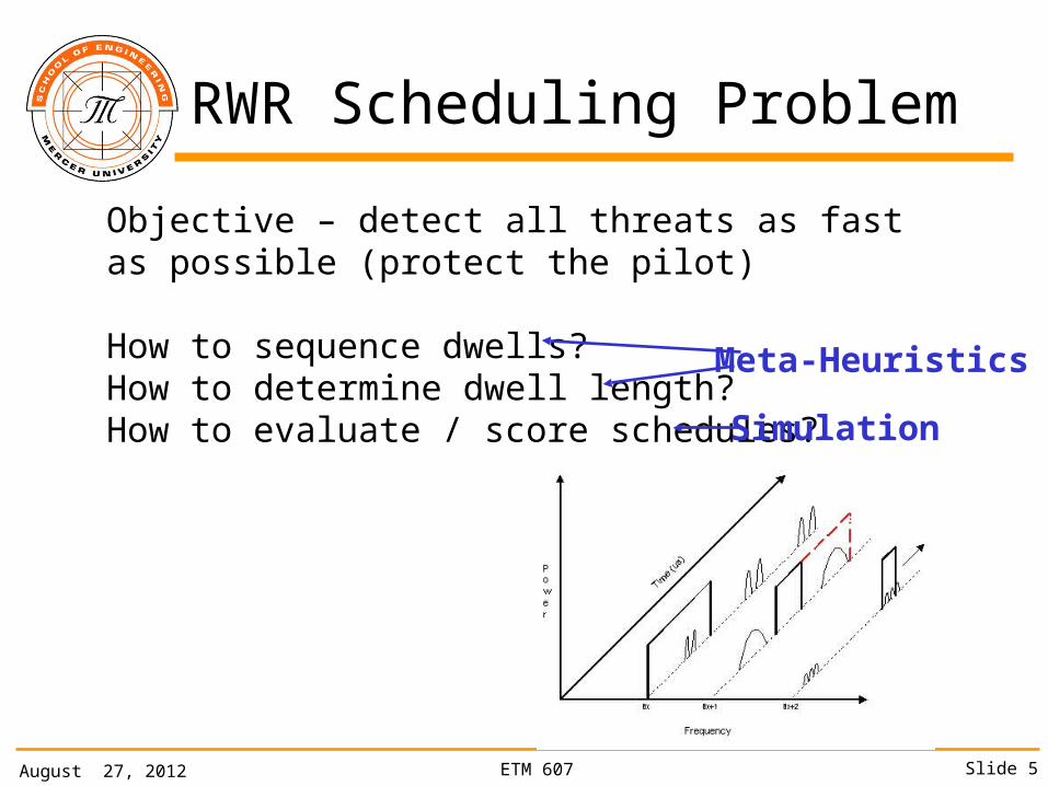
RWR Scheduling Problem
Objective – detect all threats as fast as possible (protect the pilot)
How to sequence dwells?How to determine dwell length?How to evaluate / score schedules?
Meta-Heuristics
Simulation
August 27, 2012 ETM 607 Slide 6
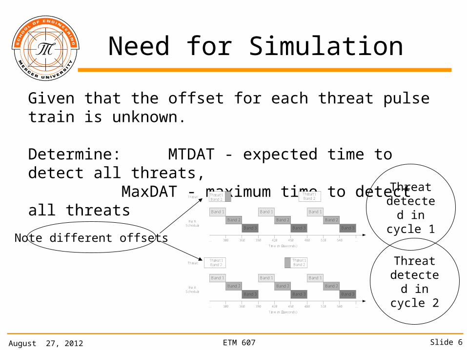
Need for Simulation
Given that the offset for each threat pulse train is unknown.
Determine: MTDAT - expected time to detect all threats, MaxDAT - maximum time to detect all threats
Threat 1Band 2
Band 1
Band 2
Band 3
Band 1
Band 2
Band 3
Band 1
Band 2
Band 3
Threat 1Band 2
300 360 390 420 450 480 510 540 ......
Time (milliseconds)
RWR Schedule
Threat
Band 1
Band 2
Band 3
Band 1
Band 2
Band 3
Band 1
Band 2
Band 3
Threat 1Band 2
Threat 1Band 2
300 360 390 420 450 480 510 540 ......
Time (milliseconds)
RWR Schedule
Threat
Note different offsets
Threat detected in
cycle 1
Threat detected in
cycle 2
August 27, 2012 ETM 607 Slide 7
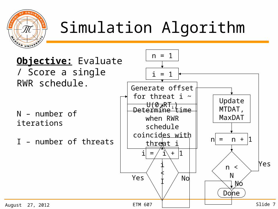
Simulation Algorithm
n = 1
i = 1
Generate offset for threat i ~ U(0,RTi)
Determine time when RWR schedule
coincides with threat i
i = i + 1
i < I
Objective: Evaluate / Score a single RWR schedule.
N – number of iterations
I – number of threatsn = n + 1
Update MTDAT, MaxDAT
n < N
Done
Yes
Yes
NoNo
August 27, 2012 ETM 607 Slide 8
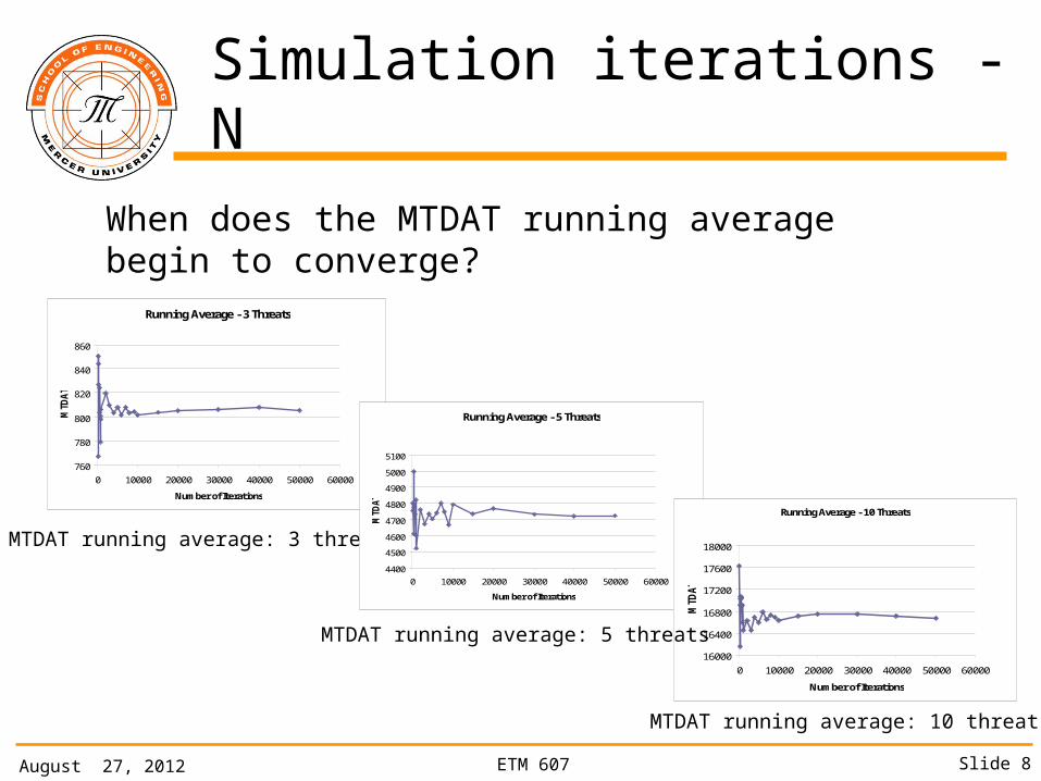
Simulation iterations - N
When does the MTDAT running average begin to converge?
Running Average - 3 Threats
760
780
800
820
840
860
0 10000 20000 30000 40000 50000 60000
Number of Iterations
MTD
AT
MTDAT running average: 3 threats
Running Average - 5 Threats
4400
4500
4600
4700
4800
4900
5000
5100
0 10000 20000 30000 40000 50000 60000
Number of Iterations
MTD
AT
Running Average - 10 Threats
16000
16400
16800
17200
17600
18000
0 10000 20000 30000 40000 50000 60000
Number of IterationsM
TDA
T
MTDAT running average: 5 threats
MTDAT running average: 10 threats
August 27, 2012 ETM 607 Slide 9
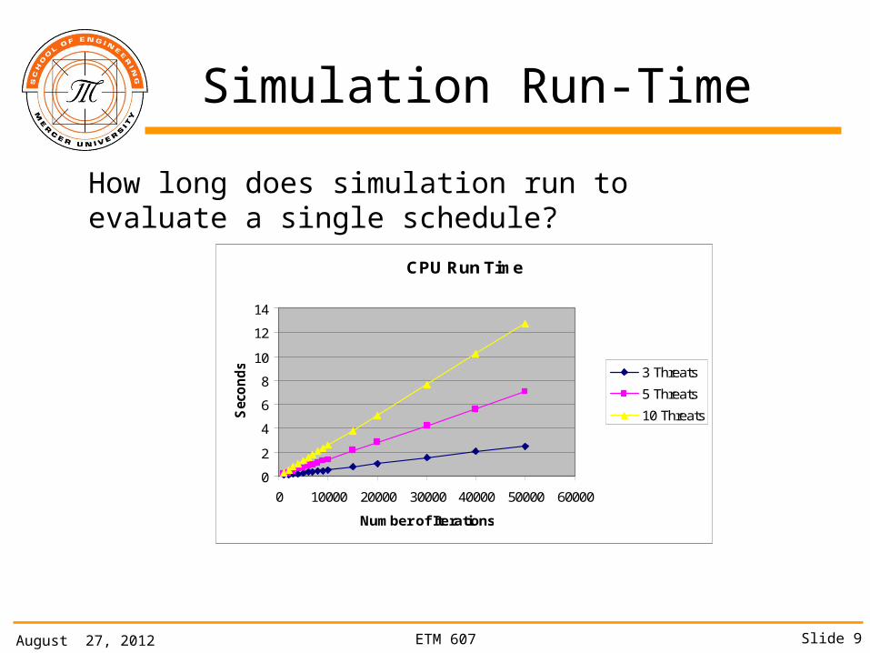
Simulation Run-Time
How long does simulation run to evaluate a single schedule?
CPU Run Time
0
2
4
6
8
10
12
14
0 10000 20000 30000 40000 50000 60000
Number of Iterations
Sec
on
ds 3 Threats
5 Threats
10 Threats
August 27, 2012 ETM 607 Slide 10
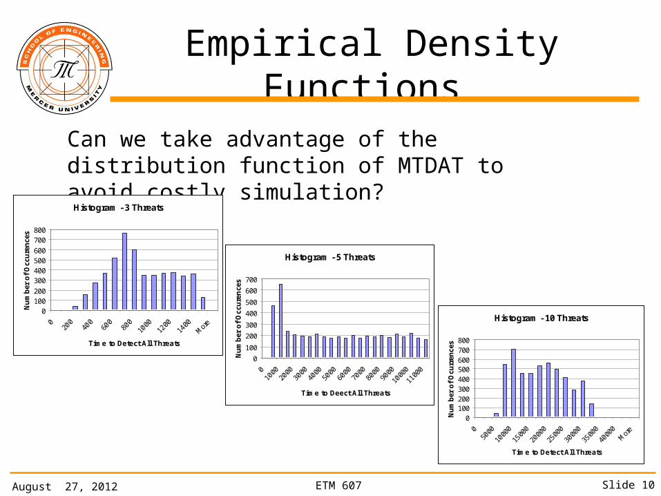
Empirical Density Functions
Can we take advantage of the distribution function of MTDAT to avoid costly simulation?
Histogram - 3 Threats
0100200
300400500600
700800
020
040
060
080
010
0012
0014
00M
ore
Time to Detect All Threats
Nu
mb
er o
f O
ccu
ren
ces
Histogram - 5 Threats
0
100
200
300
400
500
600
700
Time to Deect All Threats
Nu
mb
er o
f O
ccu
ren
ces
Histogram - 10 Threats
0100200300400500600700800
050
00
1000
0
1500
0
2000
0
2500
0
3000
0
3500
0
4000
0M
ore
Time to Detect All ThreatsN
um
ber
of
Ocu
rren
ces
August 27, 2012 ETM 607 Slide 11
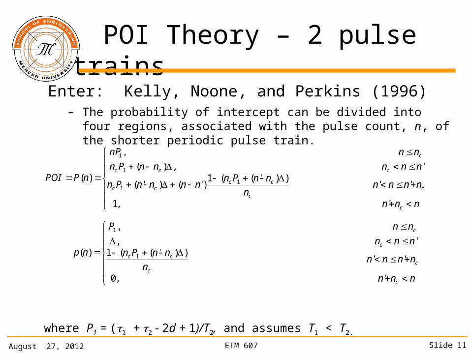
POI Theory – 2 pulse trains
Enter: Kelly, Noone, and Perkins (1996) – The probability of intercept can be divided into four regions, associated with
the pulse count, n, of the shorter periodic pulse train.
where P1 = (1 + 2 - 2d + 1)/T2, and assumes T1 < T2.
* Note, Kelly Noone and Perkins did not add the 1, we believe trailing edge triggered.
nnn
nnnnn
nnPnnnnnPn
nnnnnPn
nnnP
nPPOI
c
cc
cccc
ccc
c
',1
''))'((1
)'()'(
',)(
,
)( 11
1
1
nnn
nnnnn
nnPnnnn
nnP
np
c
cc
cc
c
c
',0
''))'((1
',
,
)( 1
1
August 27, 2012 ETM 607 Slide 12
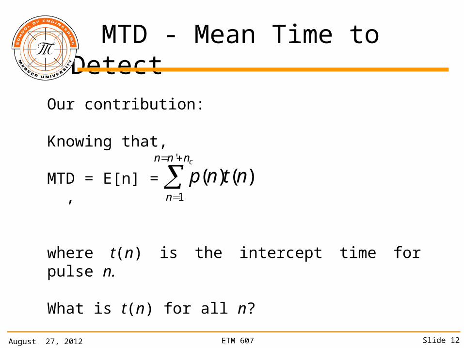
MTD - Mean Time to Detect
Our contribution:
Knowing that,
MTD = E[n] = ,
where t(n) is the intercept time for pulse n.
What is t(n) for all n?
cnnn
n
ntnp'
1
)()(
August 27, 2012 ETM 607 Slide 13
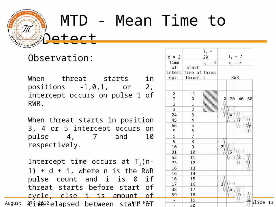
MTD - Mean Time to Detect
Observation:
When threat starts in positions -1,0,1, or 2, intercept occurs on pulse 1 of RWR.
When threat starts in position 3, 4 or 5 intercept occurs on pulse 4, 7 and 10 respectively.
Intercept time occurs at T1(n-1) + d + i, where n is the RWR pulse count and i is 0 if threat starts before start of cycle, else i is amount of time elapsed between start of RWR pulse and start of threat.
d = 2 T2 = 20 T1 = 7
Time of Intercep
t Start Time of Threat
Threat RWR
2 -1
2 0 0 20 40 602 1
1
3 24
24 3
7
45 4 1066 5
9 6 9 7 9 8
2
10 9 5
31 10
8
52 11 1173 12
16 13 16 14 16 15
3
17 16 6
38 17
9
59 18 12- 19
- 20

August 27, 2012 ETM 607 Slide 14
MTD - Mean Time to Detect
Expected times t(n) per cycle n:
where is an indeterminate error bounded by:
and, MTD =
where E is the total error bounded by:
,12
)1()(21
11
1
1
d
idnTnt
d
i
nn v
,)1()( 1'
dnTntnnnn vc
.1
1
1
d
i
i
Entnpcnnn
n
'
1
)()(
.)1(1
11
1
d
ic
iPnE
August 27, 2012 ETM 607 Slide 15
MTD - Mean Time to Detect
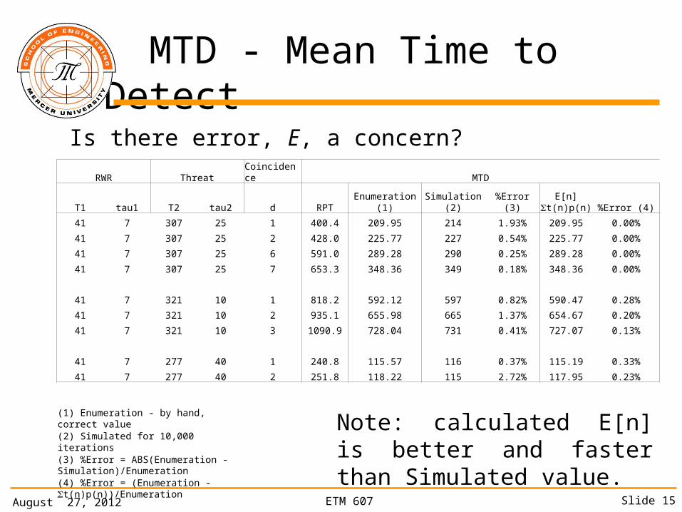
Is there error, E, a concern?RWR Threat Coincidence MTD
T1 tau1 T2 tau2 d RPT Enumeration (1) Simulation (2) %Error (3)E[n]
t(n)p(n) %Error (4)
41 7 307 25 1 400.4 209.95 214 1.93% 209.95 0.00%
41 7 307 25 2 428.0 225.77 227 0.54% 225.77 0.00%
41 7 307 25 6 591.0 289.28 290 0.25% 289.28 0.00%
41 7 307 25 7 653.3 348.36 349 0.18% 348.36 0.00%
41 7 321 10 1 818.2 592.12 597 0.82% 590.47 0.28%
41 7 321 10 2 935.1 655.98 665 1.37% 654.67 0.20%
41 7 321 10 3 1090.9 728.04 731 0.41% 727.07 0.13%
41 7 277 40 1 240.8 115.57 116 0.37% 115.19 0.33%
41 7 277 40 2 251.8 118.22 115 2.72% 117.95 0.23%
(1) Enumeration - by hand, correct value
(2) Simulated for 10,000 iterations
(3) %Error = ABS(Enumeration - Simulation)/Enumeration
(4) %Error = (Enumeration - t(n)p(n))/Enumeration
Note: calculated E[n] is better and faster than Simulated value.

August 27, 2012 ETM 607 Slide 16
Summary and Limitations
Summary:• An innovative closed form approach for determining the mean time for coincidence of periodic pulse trains has been developed using POI theory and insight on the coincidence of periodic pulse trains.
• The approach is computationally faster and more accurate than a previous presented Monte Carlo simulation approach.
Limitations:• This method is limited to threats which exhibit strictly periodic pulse train behavior (e.g. rotating beacons).• Still need method to determine MaxDAT
Future:• An enumerative approach is being evaluated for non-periodic pulse trains.