August 27, 2012 ETM 607 Slide 1
ETM 607Application of Monte Carlo
Simulation:Scheduling Radar Warning
Receivers (RWRs)
Scott R. Schultz Mercer University
August 27, 2012 ETM 607 Slide 2
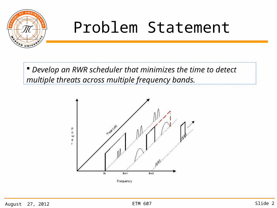
Problem Statement
Develop an RWR scheduler that minimizes the time to detect multiple threats across multiple frequency bands.

August 27, 2012 ETM 607 Slide 3
RWR Scheduling Definitions
Pulse Width (PW)
Revisit Time (RT)
IlluminationTime (IT)
Pulse RepetitionInterval (PRI)
Beam Width (BW)
Definitions:
Revisit Time (RT) – time to rotate 360 degrees (rotating radar)
Illumination Time (IT) – function of RT and BW
Pulse Width (PW) – length of time while target is energized
Pulse Repetition Interval (PRI) – time between pulses
Time
August 27, 2012 ETM 607 Slide 4
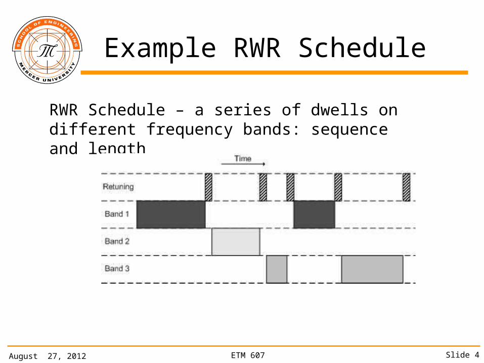
Example RWR Schedule
RWR Schedule – a series of dwells on different frequency bands: sequence and length
August 27, 2012 ETM 607 Slide 5
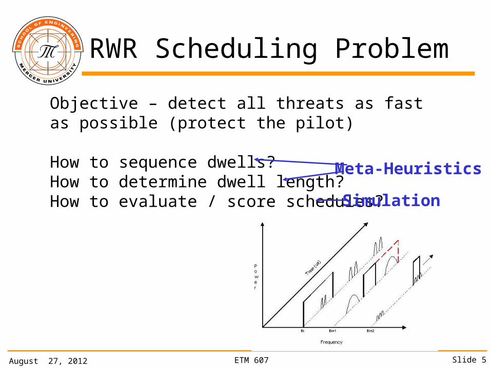
RWR Scheduling Problem
Objective – detect all threats as fast as possible (protect the pilot)
How to sequence dwells?How to determine dwell length?How to evaluate / score schedules?
Meta-Heuristics
Simulation
August 27, 2012 ETM 607 Slide 6
Need for Simulation
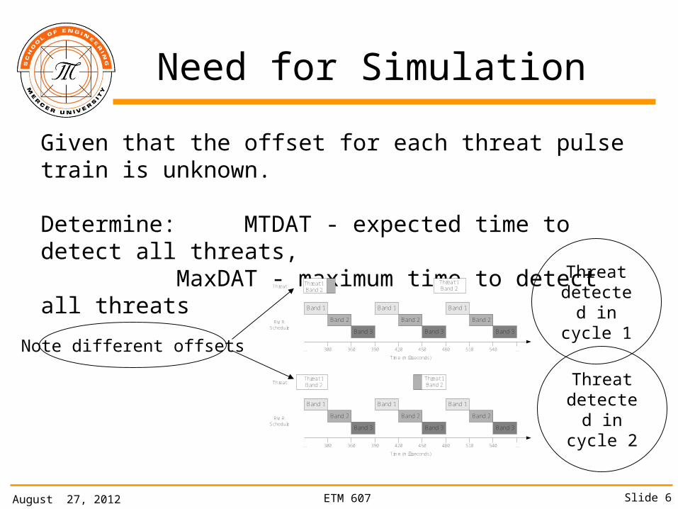
Given that the offset for each threat pulse train is unknown.
Determine: MTDAT - expected time to detect all threats, MaxDAT - maximum time to detect all threats
Threat 1Band 2
Band 1
Band 2
Band 3
Band 1
Band 2
Band 3
Band 1
Band 2
Band 3
Threat 1Band 2
300 360 390 420 450 480 510 540 ......
Time (milliseconds)
RWR Schedule
Threat
Band 1
Band 2
Band 3
Band 1
Band 2
Band 3
Band 1
Band 2
Band 3
Threat 1Band 2
Threat 1Band 2
300 360 390 420 450 480 510 540 ......
Time (milliseconds)
RWR Schedule
Threat
Note different offsets
Threat detected in
cycle 1
Threat detected in
cycle 2
August 27, 2012 ETM 607 Slide 7
Simulation Algorithm
n = 1
i = 1
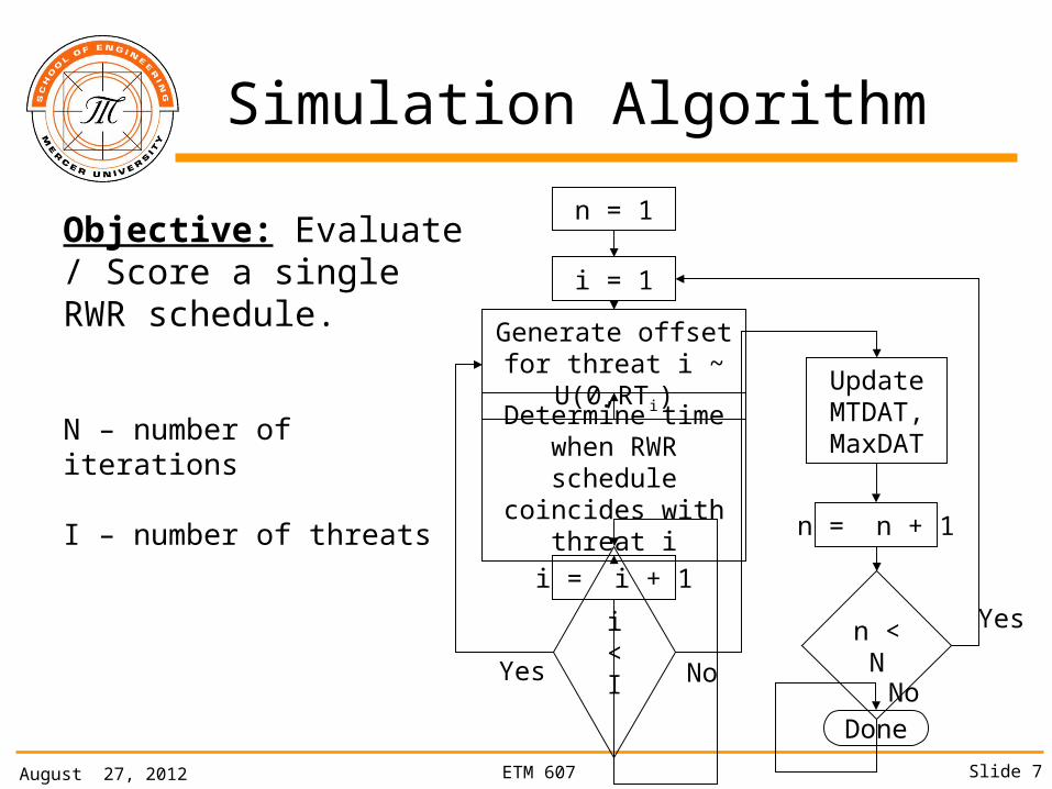
Generate offset for threat i ~ U(0,RTi)
Determine time when RWR schedule
coincides with threat i
i = i + 1
i < I
Objective: Evaluate / Score a single RWR schedule.
N – number of iterations
I – number of threatsn = n + 1
Update MTDAT, MaxDAT
n < N
Done
Yes
Yes
NoNo
August 27, 2012 ETM 607 Slide 8
Simulation iterations - N
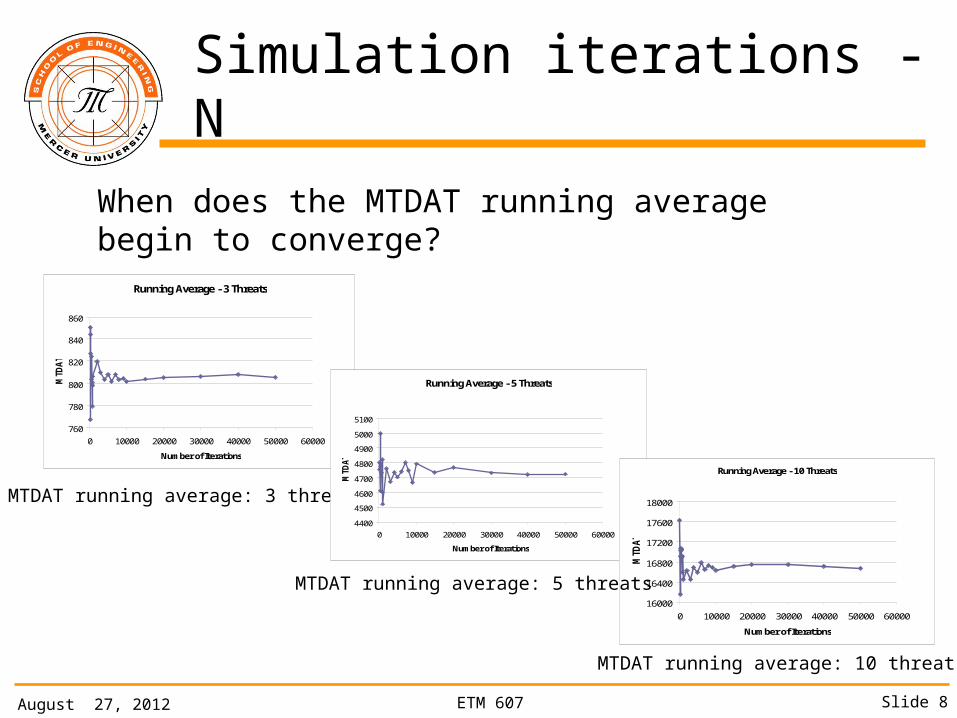
When does the MTDAT running average begin to converge?
Running Average - 3 Threats
760
780
800
820
840
860
0 10000 20000 30000 40000 50000 60000
Number of Iterations
MTD
AT
MTDAT running average: 3 threats
Running Average - 5 Threats
4400
4500
4600
4700
4800
4900
5000
5100
0 10000 20000 30000 40000 50000 60000
Number of Iterations
MTD
AT
Running Average - 10 Threats
16000
16400
16800
17200
17600
18000
0 10000 20000 30000 40000 50000 60000
Number of IterationsM
TDA
T
MTDAT running average: 5 threats
MTDAT running average: 10 threats
August 27, 2012 ETM 607 Slide 9
Simulation Run-Time
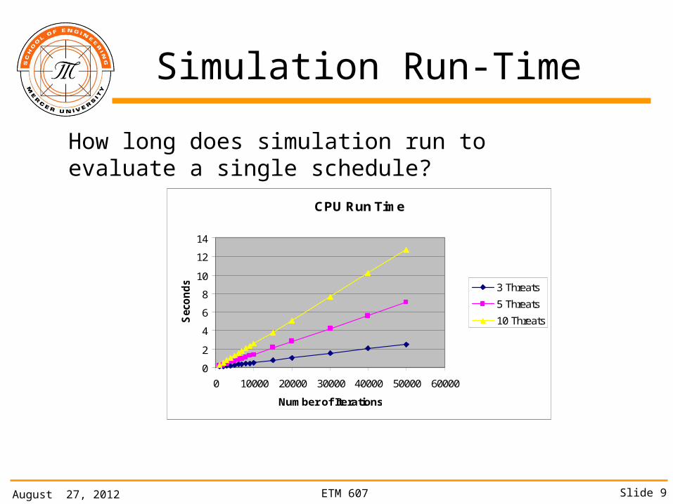
How long does simulation run to evaluate a single schedule?
CPU Run Time
0
2
4
6
8
10
12
14
0 10000 20000 30000 40000 50000 60000
Number of Iterations
Sec
on
ds 3 Threats
5 Threats
10 Threats
August 27, 2012 ETM 607 Slide 10
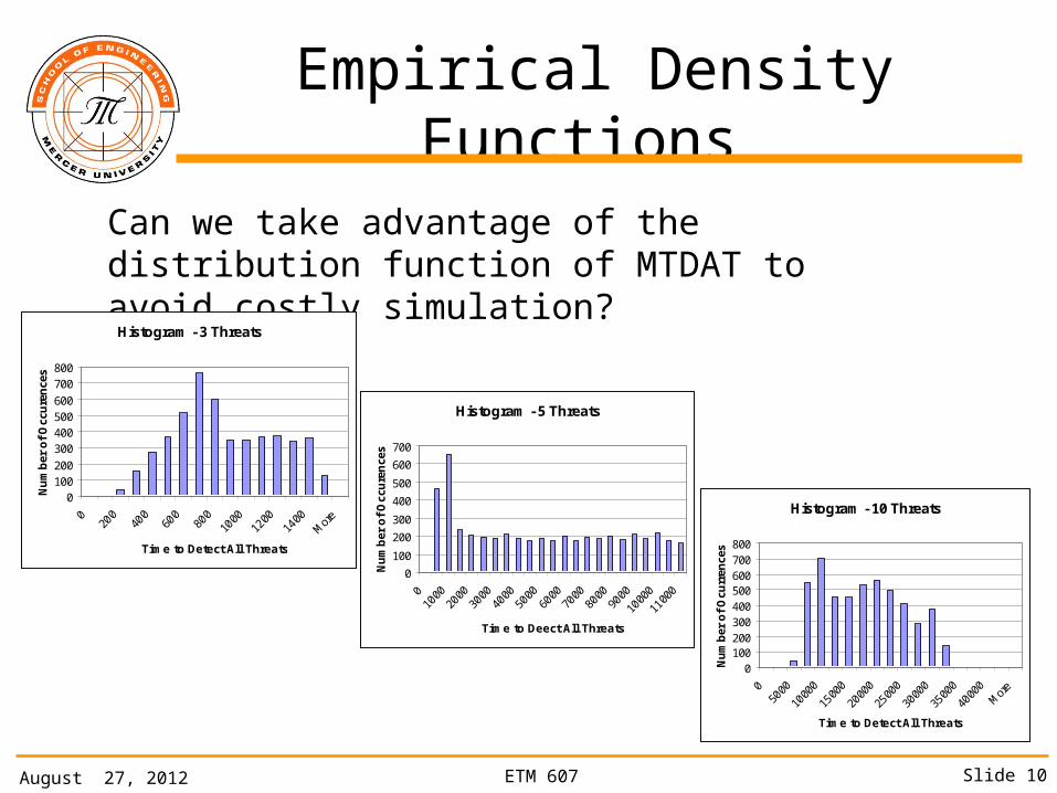
Empirical Density Functions
Can we take advantage of the distribution function of MTDAT to avoid costly simulation?
Histogram - 3 Threats
0100200
300400500600
700800
020
040
060
080
010
0012
0014
00M
ore
Time to Detect All Threats
Nu
mb
er o
f O
ccu
ren
ces
Histogram - 5 Threats
0
100
200
300
400
500
600
700
Time to Deect All Threats
Nu
mb
er o
f O
ccu
ren
ces
Histogram - 10 Threats
0100200300400500600700800
050
00
1000
0
1500
0
2000
0
2500
0
3000
0
3500
0
4000
0M
ore
Time to Detect All ThreatsN
um
ber
of
Ocu
rren
ces
August 27, 2012 ETM 607 Slide 11
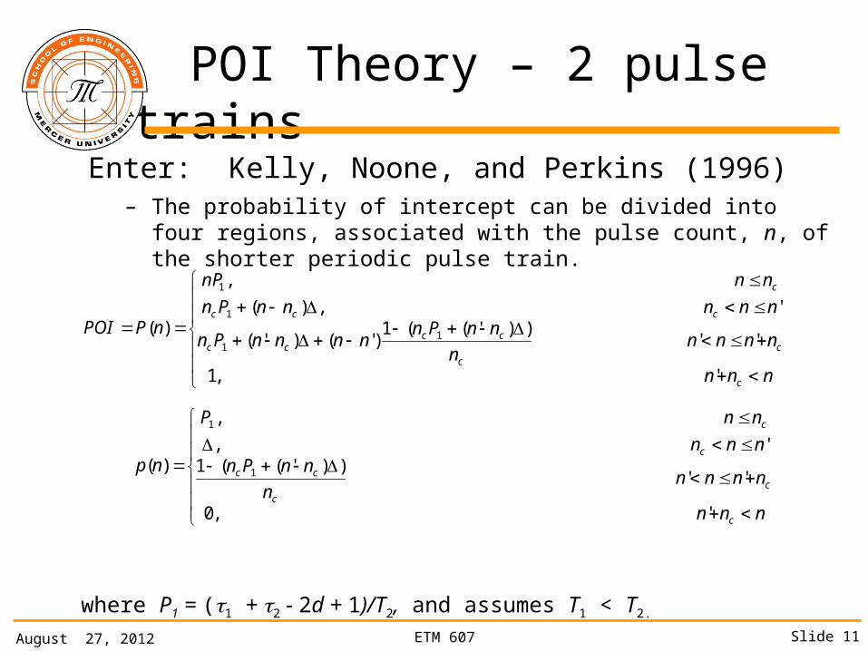
POI Theory – 2 pulse trains
Enter: Kelly, Noone, and Perkins (1996) – The probability of intercept can be divided into four regions, associated with
the pulse count, n, of the shorter periodic pulse train.
where P1 = (1 + 2 - 2d + 1)/T2, and assumes T1 < T2.
* Note, Kelly Noone and Perkins did not add the 1, we believe trailing edge triggered.
nnn
nnnnn
nnPnnnnnPn
nnnnnPn
nnnP
nPPOI
c
cc
cccc
ccc
c
',1
''))'((1
)'()'(
',)(
,
)( 11
1
1
nnn
nnnnn
nnPnnnn
nnP
np
c
cc
cc
c
c
',0
''))'((1
',
,
)( 1
1
August 27, 2012 ETM 607 Slide 12
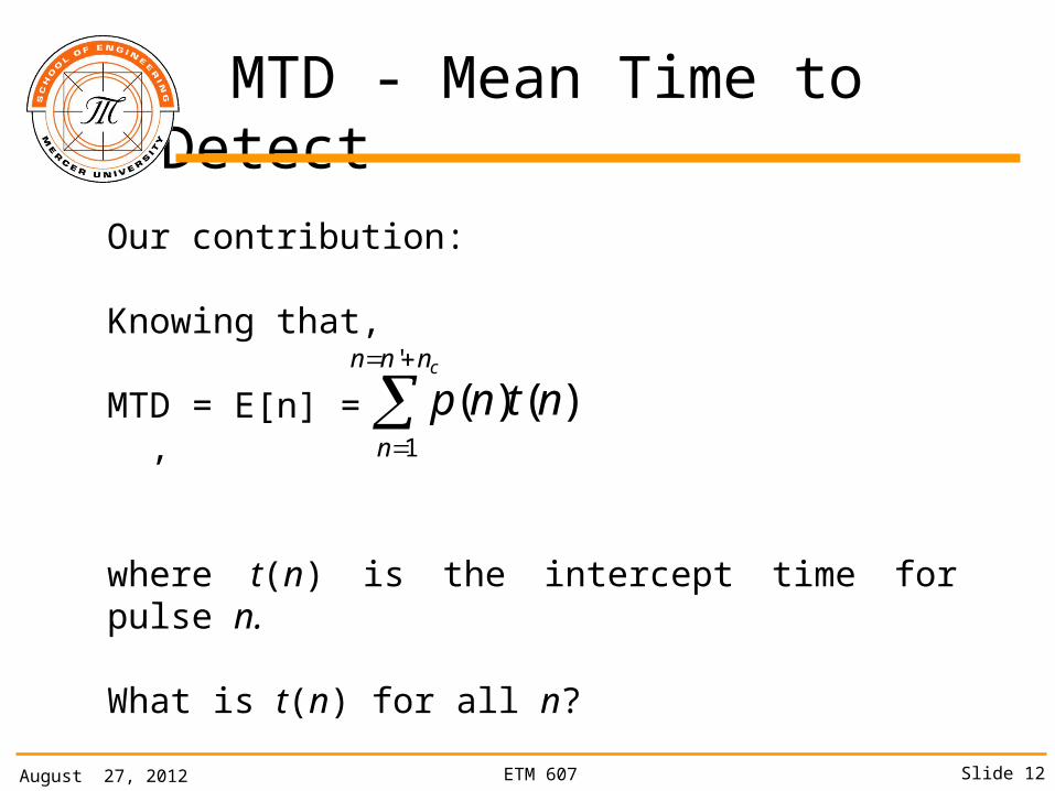
MTD - Mean Time to Detect
Our contribution:
Knowing that,
MTD = E[n] = ,
where t(n) is the intercept time for pulse n.
What is t(n) for all n?
cnnn
n
ntnp'
1
)()(
August 27, 2012 ETM 607 Slide 13
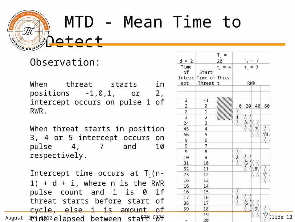
MTD - Mean Time to Detect
Observation:
When threat starts in positions -1,0,1, or 2, intercept occurs on pulse 1 of RWR.
When threat starts in position 3, 4 or 5 intercept occurs on pulse 4, 7 and 10 respectively.
Intercept time occurs at T1(n-1) + d + i, where n is the RWR pulse count and i is 0 if threat starts before start of cycle, else i is amount of time elapsed between start of RWR pulse and start of threat.
d = 2 T2 = 20 T1 = 7
Time of Intercep
t Start Time of Threat
Threat RWR
2 -1
2 0 0 20 40 602 1
1
3 24
24 3
7
45 4 1066 5
9 6 9 7 9 8
2
10 9 5
31 10
8
52 11 1173 12
16 13 16 14 16 15
3
17 16 6
38 17
9
59 18 12- 19
- 20

August 27, 2012 ETM 607 Slide 14
MTD - Mean Time to Detect
Expected times t(n) per cycle n:
where is an indeterminate error bounded by:
and, MTD =
where E is the total error bounded by:
,12
)1()(21
11
1
1
d
idnTnt
d
i
nn v
,)1()( 1'
dnTntnnnn vc
.1
1
1
d
i
i
Entnpcnnn
n
'
1
)()(
.)1(1
11
1
d
ic
iPnE
August 27, 2012 ETM 607 Slide 15
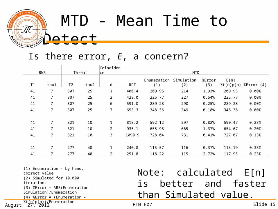
MTD - Mean Time to Detect
Is there error, E, a concern?RWR Threat Coincidence MTD
T1 tau1 T2 tau2 d RPT Enumeration (1) Simulation (2) %Error (3)E[n]
t(n)p(n) %Error (4)
41 7 307 25 1 400.4 209.95 214 1.93% 209.95 0.00%
41 7 307 25 2 428.0 225.77 227 0.54% 225.77 0.00%
41 7 307 25 6 591.0 289.28 290 0.25% 289.28 0.00%
41 7 307 25 7 653.3 348.36 349 0.18% 348.36 0.00%
41 7 321 10 1 818.2 592.12 597 0.82% 590.47 0.28%
41 7 321 10 2 935.1 655.98 665 1.37% 654.67 0.20%
41 7 321 10 3 1090.9 728.04 731 0.41% 727.07 0.13%
41 7 277 40 1 240.8 115.57 116 0.37% 115.19 0.33%
41 7 277 40 2 251.8 118.22 115 2.72% 117.95 0.23%
(1) Enumeration - by hand, correct value
(2) Simulated for 10,000 iterations
(3) %Error = ABS(Enumeration - Simulation)/Enumeration
(4) %Error = (Enumeration - t(n)p(n))/Enumeration
Note: calculated E[n] is better and faster than Simulated value.

August 27, 2012 ETM 607 Slide 16
Summary and Limitations
Summary:• An innovative closed form approach for determining the mean time for coincidence of periodic pulse trains has been developed using POI theory and insight on the coincidence of periodic pulse trains.
• The approach is computationally faster and more accurate than a previous presented Monte Carlo simulation approach.
Limitations:• This method is limited to threats which exhibit strictly periodic pulse train behavior (e.g. rotating beacons).• Still need method to determine MaxDAT
Future:• An enumerative approach is being evaluated for non-periodic pulse trains.


