ethnic diversity and international trade
TRANSCRIPT

Ethnic Diversity and International Trade
Evidence from panel data in the EU
Master Thesis
Nikki Schellekens
456828
Erasmus School of Economics
Supervisor: Benoit Crutzen
July 2017

2
Abstract Ethnic diversity is defined as the variety of different ethnic groups within a society. Conflicts
can be caused by more and diverse nationalities within a country although it can also, amongst
others, enhance international trade through two channels. First, boosting imports, immigrants
demand some of their home-country products. Second, immigrants decrease the transactions
costs with respect to uncertainty and incomplete information, which in turn increases exports.
It is referred to as migrants possessing superior foreign-market-intelligence, which nationals do
not own, therefore engaging in market creation; being able to open up to other markets abroad.
Several ways are accessible to measure ethnic diversity, where the fractionalization and
polarization index are considered to be close proxies. In this study a polarization index is created
as a measure for ethnic diversity, dividing the population by foreign countries they were born
and the depth of cleavage being proxied by the six cultural dimensions of Hofstede. This study
aims to investigate whether ethnic diversity affects international trade using panel data from
2000 to 2017 of the 28 member countries of the EU. The results show the relationship to be
positive, implying ethnic diversity to increase international trade, dominated by the foreign
good demand channel over the market creation effect.
This study contributes to the existing literature for making it possible to perform a panel
data study including fixed effect, when calculating the yearly values for ethnic diversity instead
of time invariant values. Moreover, it is the first empirical study to analyze the impact of ethnic
diversity on the aggregate of international trade.

3
Table of content Abstract ...................................................................................................................................... 2
Table of content .......................................................................................................................... 3
Introduction ................................................................................................................................ 4
Theoretical framework ............................................................................................................... 5
Migration and Trade ................................................................................................................... 6
Literature review ........................................................................................................................ 7
Ethnic diversity and economic performance .............................................................................. 9
Hofstede’s cultural dimensions ................................................................................................ 10
Hypothesis - Ethnic diversity and international trade .............................................................. 12
Data and methodology ............................................................................................................. 13
Data ....................................................................................................................................... 13
Descriptive statistics ............................................................................................................. 17
Comparison of the different proxies for ethnic diversity...................................................... 19
Random versus fixed effects ................................................................................................. 22
Model specification .............................................................................................................. 23
Endogeneity issues ............................................................................................................... 25
Robustness ............................................................................................................................ 25
Causality ............................................................................................................................... 27
Results ...................................................................................................................................... 27
Robustness checks ................................................................................................................ 31
Causality ............................................................................................................................... 32
Limitations ............................................................................................................................... 32
Conclusion ................................................................................................................................ 34
References ................................................................................................................................ 35
Appendix .................................................................................................................................. 38
4
1. Introduction The flow of migrants over the whole world is increasing in volume every year (World Bank,
2017). This is amongst others due to the world getting more globalized and transportation and
communication is faster and easier than ever before. Moreover, firms are becoming
multinationals, their employees work from over the world, having different nationalities and
cultures. This creates a multicultural society where different cultures meet that might lead to
clashes and conflicts within society and within firms but, on the other hand, diversity within the
firm opens up foreign markets, both for imports and exports, that in turn increases welfare
globally for the very same society.
According to the Central Bureau of Statistics (CBS) of the Netherlands, almost 70% of
the population experiences tensions between different groups of migrants in the Netherlands
(CBS, 2017). Moreover, the recent stream of refugees from amongst others Syria, has led to
heavy discussions and conflicts within the Netherlands. The refugee crisis is affecting Europe
as a whole and has given rise to an emergency procedure in 2015 by the European Union (EU)
aiming to control the abundance of migrants. Concluding from these facts and incidents,
Europeans are mostly pessimistic about more diversity within society, also called ethnic
diversity.
Refugees are only a small share of the total proportion of foreigners in Europe; the
biggest part exists of work and family migrants. In general, natives only regard the negative
side effects of the arrival of migrants, however, they should also consider the benefits it bring
and therefore, these positive consequences should be highlighted more. For example, studies
have already shown that ethnic diversity enhances economic growth (Alesina & La Ferrara,
2005), and ethnic diversity within firms leads to more diverse idea generation, stimulating
innovation (McLeod & Lobel, 1992).
Moreover, migrants have experienced a different history which causes them to own a
different background, culture etc. that adds valuable new knowledge to society. With the use of
this supplementary knowledge and their networks, new foreign markets can be opened up for
trade, which enhances exports. Besides, the inflow of migrants generates a demand for foreign
products before unknown in the destination country. Thus, imports increase and the product
scope of countries broadens too, which increases welfare since consumers, overall, have love
of variety.
This study aims to investigate the effect of ethnic diversity on the aggregate of international
trade. The first section elaborates on theoretic models explaining the migration-trade nexus,
followed by an intuitive explanation and afterwards the empirical evidence in the literature

5
review. Thereafter, ethnic diversity is introduced and the multiple ways to measure it are
explained. In this study, I develop my own index that is introduced in the fifth section and
explained into more detail in the following section. The hypothesis is stated in section seven
after which the data and methodology part follows. The subsection about data explains the index
I created theoretically and the results are presented in section nine extended by the limitations
of the study in section ten. Lastly, the study ends with a conclusion of the whole.
2. Theoretical framework As assumptions of different theoretical models explaining the relationship between migration
and international trade are variant, opposing results are found. The two are either find to be
complements or substitutes, which is explained into more detail in this section.
Mundell (1957) introduced the relationship between migration and international trade
extending Samuelson’s factor-price equalization (Samuelson, 1948). He shows that an increase
in trade impediments drives factors, in this case labor, to move and on the other hand, labor
mobility restrictions stimulate trade and lead to (a tendency of) both factor- and commodity-
price equalization. In other words, international trade and migration are explained to be
substitutes. However, Markusen (1983) changes the assumptions of Mundell (1957) such that
the model becomes more realistic and other market imperfections come into place. Such market
imperfections include returns to scale, imperfect competition, production and factor taxes, and
differences in production technology that causes trade and factor movements to be
complements.
The Ricardian model is another famous trade model explaining the pattern of trade by
the comparative advantage of countries based on differences in technology. The Ricardian
model normally has only one factor of production which is labor. When a free trade policy is
conducted, the country exports the good it can produce most efficiently and all countries benefit
from free trade, even when a country has an absolute advantage in the production of all goods.
If free movement of labor is also facilitated, labor flows to the industry whose export product
is most factor intensive, because in the more productive and efficient industry, the factor reward
is higher, which attracts labor. Thus, this model explains a positive relation between trade and
factor movements and therefore, regards the two as complements.
In the Heckscher-Ohlin trade model, trade does not occur due to differences in
technology as in the Ricardian, yet due to differences between factor endowments. The more
abundant a country is in a particular production factor, being labor or capital, the relatively
6
cheaper that factor is. The country has a comparative advantage in the good which requires
relatively more of the abundant factor and produces more of this good. For this reason, the
country exports the product which requires relatively more of the abundant factor, and it import
other ones. This, again, leads to factor-price equalization as explained in the Ricardian models
and as trade leads to equal prices, the incentives to move decreases as the wages converge, thus
trade and migration are substitutes. The other way around, without trade in goods, factor price
equalization would result only if factors are traded freely; since factor price equalization is
observed in the case of free goods trade, as well as in the case of free factor trade, it can be
concluded that free goods trade and free factor trade are perfect substitutes.
Other models explaining the relationship to be complementarity base their results on the
assumption of increasing returns to scale. Experiencing both free trade and increasing returns
to scale, countries optimize welfare by specializing in one good in order to gain from
specialization, which both countries do. The reward of the factor intensively used in that sector
rises because of the assumption of increasing returns to scale. Thus, there is an incentive for
labor to move which is followed by an upswing in production and therefore an increase in trade.
In other words, the model finds the relation between migration and trade to be complementary.
I have now elaborated on the theoretical models explaining the relationship between
migration and international trade. The next section continues with describing the relationship
more intuitively.
3. Migration and Trade Two channels explain the migration trade nexus where the first is effecting imports and the
second impacts both exports and to a lesser extent imports. First, boosting imports, immigrants
demand some of their home-country products. Second, immigrants can decrease the
transactions costs with respect to uncertainty and incomplete information, which in turn reduce
transaction costs of bilateral trade with those countries. Moreover, the networks the migrants
have acquired enhances trade which is defined by Girma and Yu (2002) as individual-specific
whereas the gained knowledge is being referred to as non-individual-specific. As the import
boosting channel seems more intuitive, only the latter is going to be explained in more detail.
International trade requires knowledge about, amongst others, the market, the culture
and the language of the trading country in order to minimize costs and failures. However, such
knowledge is difficult to acquire because of the distance, literally and figuratively, and it can
even be impossible to learn, as for example culture is subjective. This makes research into the

7
foreign country costly especially in the case of more different countries in terms of culture,
policy and economy. Migrants can therefore act as a bridge or a weak tie for providing
information the firm requires beneficial for performing business with the migrant’s originate
country or a country similar to that. Wagner, Head and Reis (2002) define this knowledge as
superior foreign-market-intelligence the migrants possess, that the nationals do not own, in
which the more different the countries are, the more valuable the weak ties. Because,
international trade increases the more of these (different) weak ties exists. In other words, the
more migrants from different countries, the more the export market can be expanded which
stimulates international trade. Egger, Von Ehrlich and Nelson (2012) specify that migrants
engage in market creation, i.e. being able to open up to other foreign markets.
However in their study they find a certain threshold of migrants after which the effect on
international trade is expected to decline or even disappear. As soon as the connection to a
certain country has already been formed and trade with that foreign market is established, not
much more of those migrants are needed anymore to keep increasing international trade. The
threshold level is estimated at a level of around 4,000 immigrants (Egger, Ehrlich, Von, &
Nelson, 2012). This mechanism is confirmed by an empirical paper of Genc, Gheasi, Nijkamp
and Poot (2012), where the elasticities of the growing stock of immigration is found to decrease
over time, implying that the marginal benefit of immigration is decreasing.
4. Literature review After explaining the theoretical models and a more intuitive explanation, this section elaborates
on the empirical evidence of these models and mechanisms. Most empirical studies concerning
the immigration trade relationship, examine gravity models starting with Gould (1994) finding
a complementary relationship. Moreover, Genc et al. (2012), conclude in their study that on
average, an increase of immigration of 10 percent increases international trade with 1.5 percent.
These results confirm the results found by Head and Reis (1998) over an earlier time frame
using data from Canada, determining a 10 percent increase in immigration causes a 1 percent
increase in exports and a 3 percent increase in import. The increase in imports originates from
immigrants demanding products of their home country and the rise in exports and also partially
behind imports is explained by the market creation effect.
Moreover, Parsons (2005) also differentiates between exports and imports in his
empirical study, representing respectively the market creation and foreign-good demand
channel. He finds that immigrants have a positive influence on both imports and exports in the

8
countries analyzed, being the EU-15. It is found that a 10% rise in immigration increases the
exports of these countries by 1.2% and the imports by 1.4%, implying that the effect on
international trade is dominated by the demand for the native goods of the immigrants over the
effect of the reduction in transaction costs.
Girma and Yu (2002) find, based on data in the UK, that exports are mostly driven
through the non-individual-specific channel. In other words, creating new knowledge the
immigrants possess from their home countries' market, rather than the networks and personal
contacts they have acquired, stimulates exports. They separate commonwealth (CWC) and non-
commonwealth countries (NCWC) in which trade with the former emerges from the network
channel as the characteristics and history with the CWC are almost similar to the UK. The
export data reveals a positive relationship between the stock of immigrants from NCWC and
UK's exports, whereas they did not find any trade-enhancing effect from CWC immigrants.
Thus, trade is driven by the non-individual-specific channel, rather than the business
connections or personal contacts they own. The import data shows the effect between CWC
and immigration to be negative, implying the two to be substitutes. However it is mentioned
that the CWC immigrant stock in the UK is relatively large, which could have made it cheaper
to manufacture the ‘home’-goods the immigrants demand itself rather than importing them, due
to economies of scale for production, that might have biased the results.
Not many empirical studies have found a substitutional relationship between migration
and trade. However, Peters (2015) finds empirical support for his hypothesis that immigration
policy and international trade are rather substitutes. The findings are based on data about low-
skilled migration, as this covers most part of the migration stream. When trade is restricted, the
production of low-skilled intensive goods rises, resulting in higher wages as labor is demanded
more. Continually, firms would prefer to have a better immigration policy which stimulates
immigration, in order to decrease the pressure on the wages. On the other hand, as trade
impediments are minimized, competition will be fiercer and some firms need to shut down or
specialize in other industries, where for example production requires high-skilled labor, which
in turn reduces labor migration. However, since his study is examining migration policy instead
of migration itself, the mechanism works differently and for this reason it is not considered
further in this paper.
To conclude, various theoretical trade-migration models find either the two to be
complements or substitutes, whereas the empirical evidence mostly points to the
complementary relationship to hold. The empirical studies show that the effect of migration on
international trade, is particularly driven by imports rather than exports.

9
5. Ethnic diversity and economic performance I now have elaborated on both theoretical and empirical evidence for the relation between
migration and international trade. However, an overall migration flow or stock does not reveal
any information about the composition of this migration figure. For example, the stock of
migration might for a significant part exists of neighbor country migrants for which the
political, economic and cultural differences are only little. Then, migration will not affect
international trade as much as a more diverse stream of migrants coming from more different
and diverse countries. For this reason, it is more interesting to analyze ethnic diversity of a
country and its effect on international trade. In this section the concept and the different
measures of ethnic diversity are introduced extended by studies they are mostly used in.
Ethnic diversity is defined as the variety of different ethnic groups within a country.
Most empirical studies using ethnic diversity have focused on the relationship with economic
performance (Easterly & Levine, 1997) (Alesina & La Ferrara, 2005). On the one hand, ethnic
diversity creates a multicultural society where different cultures meet that in turn, leads to
conflicts within the society as well as within firms (Garcia-Montalvo & Reynal-Querol, 2004).
On the other hand, diversity within the firm expands idea creation and widens the firm scope
(McLeod & Lobel, 1992). In other words, the costs of diversity include conflicts, racism,
discrimination, although the benefits are a more diverse workforce which leads to an ethnic mix
of different cultures, experiences and abilities. This in turn creates diverse idea creation,
enhancing innovation and stimulating economic growth. As measures of ethnic diversity are
mostly used in those studies, I use those measures as a basis in my study to create the index of
ethnic diversity to estimate the effect on international trade.
The first and mostly used index measuring ethnic diversity is the fractionalization index,
more specifically the ethno-linguistic fractionalization index (ELF). It measures the chance that
two randomly chosen inhabitants of a country belong to separate groups within society (Easterly
& Levine, 1997). It is the reverse of the Herfhindahl index of different groups within society
and is calculated according to the following formula:
𝐸𝐿𝐹 = 1 − ∑ 𝑠𝑖2
𝑛
𝑖=1
where s is the share of the ethnic group i in the population. Much weight is attached to the
number of groups and the ELF is maximized when its value is one, which is the case when there
exist an infinite number of groups within the country. Alesina et al. (2003) also uses this index
and groups societies based on ethnicity, language and religion and creates for each dimension
10
a separate measure for all countries. For example for ethnicity, the Netherlands is divided into
three parts being: Europeans, Muslims and former colonies.
However, many scholars have criticized the ELF and have therefore come up with other
indexes, amongst which is the polarization index, that also takes into account the differences
between the various groups in society, i.e. the depth of cleavage. This index is designed by Ray
and Esteban (1994) and is structured the following way:
𝑃(𝑠,𝑦) = 𝐾 ∑ ∑ 𝑠𝑖1+𝛼𝑠𝑗|𝑦𝑖 − 𝑦𝑗|
𝑛
𝑗=1
𝑛
𝑖=1
where K is a constant, α a constant between 0 and 1.6, s is the share of the foreign population i
or the national population j and the last term is the depth of cleavage. The last term is difficult
to measure and therefore in most studies it is presumed to be equal for all groups. Sometimes a
proxy is taken, for example the difference in mother tongue being one for similar languages and
zero for completely different ones (Fearon, 2003). The index established in the latter study
becomes the following:
𝐹 = 1 − ∑ ∑ 𝑠𝑖𝑠𝑗𝑟𝑖𝑗
𝑛
𝑗=1
𝑛
𝑖=1
where s is the share of the population i and population j and r is the difference in mother tongue
as a proxy for the depth of cleavage. Fearon (2003) finds 822 ethnic groups in 160 countries
that made up at least one percent of the country population in the early 1990’s. The index is
maximized when there are plenty of groups speaking structurally unrelated languages and the
more similar and the fewer groups are present in society the lower the fractionalization index
is.
However, English is considered a world language and many people own the skill to
speak it these days, especially the ones migrating. Moreover, language does not reveal any
information about behavioral and cultural differences. Therefore, such proxies are not accurate
enough and other measures for the cleavage depth should be considered. In this study a
completely new index is constructed including the cultural dimensions of Hofstede as a proxy
for the depth of cleavage. In the next section these dimensions are explained into more detail.
6. Hofstede’s cultural dimensions Geert Hofstede is a former Dutch professor at Maastricht University in the fields of cross-
cultural psychology and anthropology. He became famous with his self-created cultural model,
which is often being used by academics. His model includes six cultural dimensions which are

11
chosen based on outstanding characteristics of cultures of national societies (Hofstede, 1983).
The dimensions measure the relative value of the culture of nations which can be compared
with one and other. The six dimensions are individualism, power distance, masculinity,
uncertainty avoidance, long-term orientation and indulgence and are measured on a scale from
0 to 100.
Individualism measures the extent to which people feel independent and how important
the individual and its deployment is considered to be within a certain nationality. Societies
characterized with high individualism have loose ties between individuals, they look mostly
after themselves and their family and citizens identify themselves with “I”. The opposite of
individualism is collectivism which emphasizes the importance of the group and its interests.
In such societies it is important to always have harmony in order to not lose its strength. People
always identify themselves with “we”. Hofstede explains the two extreme with a metaphor from
physics: “people in an individualistic society are more like atoms flying around in a gas while
those in collectivist societies are more like atoms fixed in a crystal” (Hofstede, The six cultural
dimensions, 2017). Scores close to zero are more collectivists and close to 100 more
individualistic.
The next cultural dimension is power distance measuring the extent to which the less
powerful ranks of society accept and respect the hierarchy and therefore the people above them.
The value for the power distance is determined by the people at the bottom rather than at the
top as it is about the acceptance of the lower ranks. Societies with high power distance are
characterized with hierarchy and everybody knows their position, inequality is considered to be
normal and they tend to be more centralized. As opposed to a society with low power distance,
power is distributed equally and hierarchy does not exist, power should be used legitimately
and decentralization is more favorable. Employees work more independently as in high power
distance employees prefer to be told what and how to do their tasks.
Masculinity includes force and courage, but as the word does say it does not have
anything to do with being male, even females can be masculine. A masculine society is
characterized by toughness, big in size, victory and a separation of both genders. Work is
dominant and an acceptable excuse to neglect family. The opposite is a feminine society where
genders are emotionally more alike and where there is empathy for the weak. Traits of such a
society are about feelings and sensitivity.
Uncertainty avoidance is the extent to which the members of a national society or a
country feel threatened by unknown situations, and does not mean risk avoidance. Countries
with high uncertainty avoidance overall experience more stress and are more aggressive that

12
cannot be controlled. They feel what is different is dangerous and they need to have rules and
regulations. They tend to be more rational, structured and anxious and have distrust for the
unknown. Low certainty avoidance societies are more relaxed and can handle unknown
situations better, they are not conservative and prefer to have some change. Mostly, those
countries are more entrepreneurial, have a higher level of innovation and start-ups. Deregulation
is preferred and switching jobs happens more often.
Long-term orientation has much to do with change and being conservative. Therefore,
it builds on the previous dimension. A long-term orientated country is aware of the future and
the consequences of everyday life nowadays. Preparation for the future is needed and people
adapt to certain circumstances easily. Countries want to learn from other countries to get better.
Short-term orientated cultures stick to the past and the present and do not change easily. They
are characterized by national pride, respect for traditional, fulfilling social obligations.
The last dimensions is indulgence which is about all the good things in life and is
subjective to happiness, such as enjoyment and having fun. Friends and family are very
important and you work to live and don’t live to work. An indulgent country is free and leisure
is central as opposed to a restrained country where freedom is limited and work is more
important. Moreover, they are more pessimistic and introvert.
All the information about the six dimension is acquired from the website of Geert
Hofstede (Hofstede, The six cultural dimensions, 2017). The values for each dimension and for
each country are based on comparisons with other countries and therefore do not present an
absolute standard value but rather a relative one.
7. Hypothesis - Ethnic diversity and international trade As is mentioned before, the stock or flow of migrants and in particular immigrants does not
reveal any composition information. The characteristics of the migrants and to the extent they
differ from the destination country are not included, which is a loss in information as the bigger
the cultural, political and economic differences the bigger the effect is expected to be on
international trade. Moreover, migrants do not only own superior knowledge about the
origination country as well as the countries similar to that, for example neighboring countries.
Therefore, in my opinion, the relationship between ethnic diversity and the national aggregate
of international trade is more interesting to study.
To my knowledge there is no literature nor studies that have directly analyzed the
relationship of combining migration and cultural differences, i.e. ethnic diversity, on

13
international trade. Therefore, I base my predictions combing the studies about migration and
trade on the one hand and ethnic diversity and economic performance on the other. I use the
theory behind the former and the variable measures from the latter studies. Both are already
discussed and for that reason I do not elaborate on them again.
However, it should be mentioned that the indexes as a proxy for ethnic diversity, that
already exist are different and have generated different results. The division of ethnic groups as
well as the measure for the depth of cleavage vary, which develops different measures.
Therefore, the creation of another index also contributes to the existing literature but should be
examined with care.
To sum up, I use the polarization index as a measure for ethnic diversity in which the
proxy for the depth of cleavage is the average of the six Hofstede cultural dimensions. I expect
that an increase in ethnic diversity within a country leads to an increase in international trade.
Therefore the relationship is expected to be positive. The polarization index which I use in my
study is explained in more detail in the data section hereafter.
8. Data and methodology
Data In this study I use a panel dataset including the 28 member countries of the European Union
over a 17 year timespan, being from 2000 until 2016. This time span is chosen as it maximizes
the availability of data, mainly as the data I retrieved from Eurostat starts in 2000. The full list
of countries can be found in table 1 in the Appendix. The main relationship I focus on is the
relation between the national ethnic diversity on the aggregate of international trade. In this
section all the variables are explained in more detail, including the dependent, independent and
control variables and which database I used to retrieve them.
The first variable is the main dependent variable, international trade, retrieved from the
World Bank1, World Development Indicators. I took both the value in current US dollar prices
of the export and import and added these to calculate Trade. As trade is slightly skewed to the
right I transformed the variable into log form, logTrade, also for making interpretation easier
and to take care of outliers.
1 World Bank database, World Development Indicators (2017), retrieved from: http://data.worldbank.org/indicator

14
The main independent variable is the polarization index as a proxy for ethnic diversity.
I calculated the yearly index for all the 28 countries myself using data from Eurostat2 and the
Hofstede3 website. I used Eurostat to download the yearly proportions of foreign-born
population per country. I combined the formula from Ray and Esteban (1994) and Fearon
(2003) to create my own polarization index (POL). The indexes are presented as respectively
Ray and Esteban index (RE) and Fearon index (F). The RE index is the following:
𝑅𝐸 = 𝐾 ∑ ∑ 𝑠𝑖1+𝛼𝑠𝑗|𝑦𝑖 − 𝑦𝑗|
𝑛
𝑗=1
𝑛
𝑖=1
where K is a constant, α a constant between 0 and 1.6, s is the share of the population i and the
population j and the last term is the depth of cleavage. This last term is difficult to measure and
therefore in most studies it is presumed to be equal for all groups. Sometimes a proxy is taken
for this term, for example the difference in mother tongue being one for similar languages and
zero for completely different ones which is used by Fearon (2003). His index becomes:
𝐹𝑒𝑎𝑟𝑜𝑛 = 1 − ∑ ∑ 𝑠𝑖𝑠𝑗𝑟𝑖𝑗
𝑛
𝑗=1
𝑛
𝑖=1
where s is the share of the population i and population j and the r is the difference in mother
tongue as a proxy for the depth of cleavage. Leaving the first part of the equation, then in a
country with languages that are to a large extent similar to one another or where only one
language is spoken, the polarization index is close to one. On the other hand when many
different languages are spoken by a lot of groups, the value will be close to zero. To get the
index analogous to the ethnic fractionalization index, it is subtracted from 1. The maximum
value of one implies a very fractionalized country and the minimum of zero represents a country
where the same language is spoken by everyone.
As the precise values for K and α are unknown I primarily used Fearon’s index as a
basis. The depth of cleavage I use in my index, is calculated based on the six cultural dimensions
of Hofstede, according to this formula:
𝑃𝑂𝐿 = 1 − ∑ 𝑠𝑖𝑠𝑗𝑐𝑖𝑗
𝑛
𝑗=1
𝑐𝑖𝑗 =∑ |𝑦𝑐,𝑖 − 𝑦𝑐,𝑗|6
𝑐=1
600
2 Eurostat database, (2017) retrieved from: http://ec.europa.eu/eurostat/statistics-explained/index.php/Migration_and_migrant_population_statistics 3 Geert Hofstede cultural dimensions (2015), retrieved from: http://geerthofstede.com/research-and-vsm/dimension-data-matrix/

15
where s is the share of the foreign population i or the national population j and cij is the depth
of cleavage between the two. I decided to leave the summation for i and consider it as the share
of national population as otherwise I would have to calculate the cultural difference for each
combination of foreign born nationalities within a country, which would have made calculations
too extensive. Furthermore, the proportions of foreign-born populations multiplied with each
other give tiny values that should not make a difference in this study.
Cij is the sum of the absolute difference of each of the six Hofstede cultural dimensions
between the foreign and national culture. As each dimension is valued between 0 and 100 I
divide it by 600 to get to a value analogous in Fearon (2003) between zero and one. A value
close to zero indicates very different cultures and a value close to one almost similar cultures.
As some countries have missing values for at least one of the cultural dimensions, I took the
average of the countries in the same region and included those. The division of the world in
regions can be seen in table 2 in the appendix. For the countries in the regions: Africa West,
Africa East and the Arab countries, the aggregated values are taken that are retrieved from the
Hofstede website3 as those were already reported.
Moreover, I calculated a polarization index with the overall depth of cleavage using all
six dimension separately, being D1, D2, D3, D4, D5 and D6. The formula for cij then becomes:
𝑐𝑖𝑗 =|𝑦𝑖 − 𝑦𝑗|
100
where y is one of the six cultural dimensions.
Another explanatory variable used in this study, is the fractionalization index that I
calculate myself again using the foreign-born shares acquired from Eurostat1. The index from
Alesina et al. (2003) is used to calculate Frac which looks the following:
𝐹𝑟𝑎𝑐 = 1 − ∑ 𝑠𝑖2
𝑛
𝑖=1
where s is the share of all different groups i, including the foreign-born and natives.
In other regressions I retrieved data about the polarization index used in Fearon4 (2003)
and the fractionalization index from Alesina et al.5 (2003). Their indexes are time invariant and
moreover they both created the measures using data from different points in time to construct a
time invariant diversity measure for a country. I applied the value for each country into all 17
years, to still be able to perform a panel data regression to make comparison with the other
indexes feasible. Alesina et al. (2003), mention in their paper that the ethnic fractionalization is
4 Replication data retrieved from: http://web.stanford.edu/group/ethnic/publicdata/publicdata.html 5 Alesina, Alberto, et al. "Fractionalization." Journal of Economic growth 8.2 (2003): 155-194.
16
generally taken as exogenous using cross-country data and that the proportions of different
population groups are sufficiently stable over a time horizon of at least 30 years. Moreover, if
they change, their impact is only little. As their data stems from the mid-90’s it is certified to
use it up until the mid-20’s which covers the timeframe used in this study.
The control variables included in the models are logGDPcap, REER, PPP, logPop,
Barriers, Inst and Global. These acronyms stand for, respectively, the logarithm of GDP per
capita, real effective exchange rate, purchasing power parity conversion factor, the logarithm
of the population size, a variable measuring the quality of institutions and the amount of
globalization. The first four are retrieved from the World Bank Development Indicators1 and
the latter two from CESIFO.
logGDPcap is used to control for indirect influences from the level of development on
the volume of trade. The log of GDP per capita is taken again for both convenience and to
construct the distribution close to a normal distribution.
The real effective exchange rate, REER, is included to control for the stability of the
home currencies as this influences the attractiveness for trade. For example, if a currency is
devaluating it becomes attractive to import products from that country as it automatically causes
the products to be cheaper, which in turn increases international trade. The opposite is true for
an appreciation, leading to a decrease in trade which is confirmed by many empirical studies
(Auboin & Ruta, 2013). The REER is a measure of the value of a currency against a weighted
average of several other currencies divided by a price deflator or index of costs retrieved from
the World Bank1. The data takes the year 2010 as the base period.
For PPP I use the price level ratio of PPP conversion factor divided by the market
exchange rate retrieved from the World Bank1 and in short the national price level. The sign
depends on the relative level of exports and imports as a lower price level is expected to increase
exports but lower imports.
Pop1 measures the population of each country and including it in the regression controls
for the size of the country. Being a large economy has been found to negatively impact a country
its trade performance as they are better able to be self-sufficient. Larger countries, or countries
with larger populations have, ceteris paribus, more opportunities for specialization and are less
dependent on imports. This effect has been found and confirmed by several authors (Alesina &
Wacziarg, 1998) (Ram, 2009). For convenience the transformation to logPop has been made.
The well-functioning of institutions reduces the level of uncertainty and therefore,
reduce transaction costs. It is empirically confirmed by several authors that good institutions
increase international trade (Jansen & Nordås, 2004). For this reason, I include Inst as a control

17
variable in my regression model. The Institutions Climate Index6 is retrieved from the CESIFO
institute in Munich.
The measures for the extent of globalization, Global¸ is included to control for changes
in international trade due to the extent of global orientation of countries. The globalization index
is retrieved from KOF Globalization Index7 which is an index measuring economic, social, and
political integration (Dreher, 2006). The data combines actual economic flows, economic
restrictions, data on information flows, data on personal contact and data on cultural proximity.
The higher its value, the more globally oriented a country is, therefore it is expected to have a
positive relation with international trade.
The variable Barriers measures the extent of trade freedom of a country. The data is
retrieved from the index of economic freedom8 and is a composite measure of the absence of
tariff and non-tariff barriers that affect imports and exports of goods and services. It includes a
trade-weighted average tariff rate and non-tariff barriers (NTB). As the value expresses the
freedom of trade the sign is expected to be positive, the more free trade is possible the higher
international trade is expected to be.
Skilled migration has found to be enhancing trade relatively more than lower skilled or
unskilled migrant workers (Docquier & Lodigiani, 2010) (Mundra, 2005). Therefore I include
EducHigh as an interaction term with the polarization and fractionalization indexes to examine
whether the results also hold in this study. I retrieved the data from CESIFO9, using the
percentage of tertiary education in foreign born population aged 25 to 64, using ISCED 5/6 as
the definition of high skilled education.
Descriptive statistics In this section the descriptive statistics of the data used are provided and some graphs are
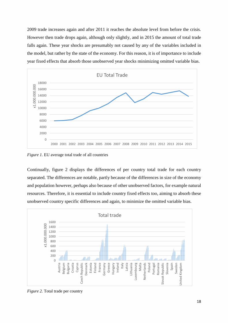
presented displaying the behavior of the variables. Figure 1 presents the amounts and the
evolution of total trade of all 28 EU member countries together. The graphs shows a steady
increase except for the years 2009, 2012 and 2015. The huge drop after 2008 represents the
global financial crisis that hit many countries, in particular the developed Western countries. In
6 DICE Database (2013), "Institutions Climate Index, 1994 - 2012", ifo Institute, Munich, online available at http://www.cesifo-group.de/DICE/fb/rN4BMUYy 7 DICE Database (2015), "Index of globalization (according to KOF), 1970 - 2011", ifo Institute, Munich, online available at http://www.cesifo-group.de/DICE/fb/4RLWQ54Hk 8 The Heritage Foundation (2017), “The index of Economic Freedom”, 2000-2017, online available at http://www.heritage.org/index/trade-freedom 9 DICE Database (2016), "Employment rates of national and foreign-born persons, by gender, 2012 - 2013", ifo Institute, Munich, online available at http://www.cesifo-group.de/DICE/fb/LKoj3H7M
18
2009 trade increases again and after 2011 it reaches the absolute level from before the crisis.
However then trade drops again, although only slightly, and in 2015 the amount of total trade
falls again. These year shocks are presumably not caused by any of the variables included in
the model, but rather by the state of the economy. For this reason, it is of importance to include
year fixed effects that absorb those unobserved year shocks minimizing omitted variable bias.
Figure 1. EU average total trade of all countries
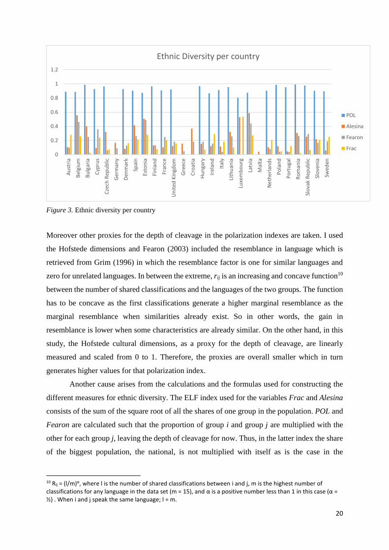
Continually, figure 2 displays the differences of per country total trade for each country
separated. The differences are notable, partly because of the differences in size of the economy
and population however, perhaps also because of other unobserved factors, for example natural
resources. Therefore, it is essential to include country fixed effects too, aiming to absorb these
unobserved country specific differences and again, to minimize the omitted variable bias.
Figure 2. Total trade per country
0
2000
4000
6000
8000
10000
12000
14000
16000
18000
2000 2001 2002 2003 2004 2005 2006 2007 2008 2009 2010 2011 2012 2013 2014 2015
x1.0
00
.00
0.0
00
EU Total Trade
0
200
400
600
800
1000
1200
1400
1600
Au
stri
a
Bel
giu
m
Bu
lgar
ia
Cro
atia
Cyp
rus
Cze
ch R
epu
blic
Den
mar
k
Esto
nia
Fin
lan
d
Fran
ce
Ge
rman
y
Gre
ece
Hu
nga
ry
Irel
and
Ital
y
Latv
ia
Lith
uan
ia
Luxe
mb
ou
rg
Mal
ta
Ne
the
rlan
ds
Po
lan
d
Po
rtu
gal
Ro
man
ia
Slo
vak
Rep
ub
lic
Slo
ven
ia
Spai
n
Swed
en
Un
ited
Kin
gdo
m
x1.0
00
.00
0.0
00
Total trade

19
Table 3 in the Appendix shows the descriptive statistics of the main variables in my study. The
indexes I created myself, POL and Frac contribute the most to cause the panel to be unbalanced
as they both have a lot of missing values. The reasons for this are twofold, first because some
countries do not report any values concerning the shares of foreign population, e.g. Germany,
Greece, Croatia and Malta. And some countries have missing observations, e.g. Cyprus,
Estonia, France, UK, Lithuania, Luxembourg, Poland and Portugal. Therefore, already four
countries are excluded from this research because of missing data and some are
underrepresented.
Moreover, the minimum and maximum values of the polarization index I created and
the index from Fearon, which I used as a basis, differ greatly. Although the minimum and
maximum values for Frac and Alesina are similar which was expected as the same formula is
used in calculating the yearly values using data and, again, Alesina being time invariant. In the
section hereafter I elaborate into more detail on the differences between the proxies used for
ethnic diversity.
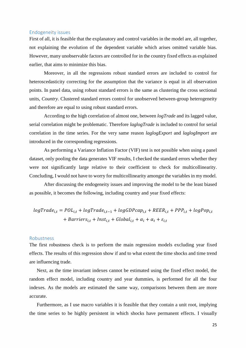
Comparison of the different proxies for ethnic diversity Figure 3 displays all indexes of all countries in the sample, to demonstrate their differences
visually. The differences are notable and some of them are outstanding, that can be explained
by several reasons, being mentioned in this subsection.
The main reason concerns the division of ethnic groups within society, as for example
the ethnic divisions for the Netherlands that Alesina et al. (2003) use in their study is; nationals,
Europeans, Muslims and former colonies. Fearon (2003) groups for example the US in; White,
Black, Hispanic and Asian and I divide society based on the nationality, i.e. country someone
is born, that includes only first generation foreigners. The maximum proportion of the latter is
at around 3% and the average lies beneath 1%. The shares of groups in Fearon (2003) and
Alesina et al. (2003) are therefore larger, although the exact shares are unfortunately not
mentioned in their papers.
20
Figure 3. Ethnic diversity per country
Moreover other proxies for the depth of cleavage in the polarization indexes are taken. I used
the Hofstede dimensions and Fearon (2003) included the resemblance in language which is
retrieved from Grim (1996) in which the resemblance factor is one for similar languages and
zero for unrelated languages. In between the extreme, rij is an increasing and concave function10
between the number of shared classifications and the languages of the two groups. The function
has to be concave as the first classifications generate a higher marginal resemblance as the
marginal resemblance when similarities already exist. So in other words, the gain in
resemblance is lower when some characteristics are already similar. On the other hand, in this
study, the Hofstede cultural dimensions, as a proxy for the depth of cleavage, are linearly
measured and scaled from 0 to 1. Therefore, the proxies are overall smaller which in turn
generates higher values for that polarization index.
Another cause arises from the calculations and the formulas used for constructing the
different measures for ethnic diversity. The ELF index used for the variables Frac and Alesina
consists of the sum of the square root of all the shares of one group in the population. POL and
Fearon are calculated such that the proportion of group i and group j are multiplied with the
other for each group j, leaving the depth of cleavage for now. Thus, in the latter index the share
of the biggest population, the national, is not multiplied with itself as is the case in the
10 Rij = (l/m)α, where l is the number of shared classifications between i and j, m is the highest number of classifications for any language in the data set (m = 15), and α is a positive number less than 1 in this case (α = ½) . When i and j speak the same language; l = m.
0
0.2
0.4
0.6
0.8
1
1.2A
ust
ria
Bel
giu
m
Bu
lgar
ia
Cyp
rus
Cze
ch R
epu
blic
Ge
rman
y
Den
mar
k
Spai
n
Esto
nia
Fin
lan
d
Fran
ce
Un
ited
Kin
gdo
m
Gre
ece
Cro
atia
Hu
nga
ry
Irel
and
Ital
y
Lith
uan
ia
Luxe
mb
ou
rg
Latv
ia
Mal
ta
Ne
the
rlan
ds
Po
lan
d
Po
rtu
gal
Ro
man
ia
Slo
vak
Rep
ub
lic
Slo
ven
ia
Swed
en
Ethnic Diversity per country
POL
Alesina
Fearon
Frac

21
fractionalization index. Since this is to be the biggest value and it gets subtracted from 1, the
polarization index generates overall, higher values. This is especially notable for the POL index.
Besides, Fearon (2003) only includes the groups being part of population of more than
1%, although I use all population shares. However, the multiplication of proportions lower than
1% generate tiny values such that it would not have made a notable difference.
To confirm the differences between the indexes, table 4 shows their correlations. Fearon
and Alesina correlate with 0.74, which is also found in Fearon (2003) and he concludes that
only a little more than half of the variation of the two measures is "shared", indicating that they
do not correlate much. POL and Frac correlate much although negatively and they correlate
little with Fearon and Alesina.
POL Frac Fearon Alesina
POL 1
Frac -0.9764 1
Fearon -0.3208 0.3301 1
Alesina -0.1541 0.0847 0.7432 1
Table 4. Correlation matrix
The most outstanding fact is that POL correlates negatively with all the other three explanatory
variables. This is structurally due to way the indexes are calculated. I demonstrate it with an
example shown in table 5. The fractionalization index attaches much weight to the number of
groups, where the more groups and of the more equal proportion, the higher fractionalized
society is calculated to be. On the other hand, the polarization index does not attach any weight
to the amount of different groups only to the relative size of the national share. The data is
mostly alike to the first two rows, in which one relatively large group and a small group exists,
however in this sample a lot of small groups. It is immediately notable that the two move in the
opposite direction. So overall, the outcomes show an intuitive transformation, however when
only considering a fraction of possibilities the evolution seems to contradict each other.
Although, notice that for convenience, I did not include the depth of cleavage in this example,
such that only the minimum values for POL are shown. The strength of the polarization index
lies in the fact that for each group the cultural distances can be included that changes the
outcomes.

22
Frac POL11
2 groups (0.95, 0.05) 0.10 0.95
2 groups (0.8, 0.2) 0.32 0.84
2 groups (0.5, 0.5) 0.50 0.75
3 groups (0.33, 0.33, 0.33) 0.67 0.78
3 groups (0.50, 0.35, 0.15) 0.605 0.75
3 groups (0.80, 0.15, 0.05) 0.40 0.84
(0.48,0.01,0.01,...) 0.76 0.95
(0.25, 0.25, 0.25, 0.25) 0.75 0.81
n groups, (1//i, 1//i,...) 1-(1/n)
Table 5. Examples of fractionalization versus polarization
The reverse effect is accelerated by the fact that the data in my sample included the member
countries of the EU. As the Schengen agreement is in force, which makes it possible for people
to move freely in the participating countries amongst which 22 of the EU member countries, it
seems fair that the population of the countries in this studies consist of higher fractions of
foreigners born in the EU countries. Moreover, all the countries being part of one union, the
EU, and being (close to) neighboring countries, they already share some culture, history,
policies etc. For this reason, the relatively low fraction of foreigners born in countries with low
cultural resemblance causes the polarization index to increase more than proportionally. On the
other hand, the high proportion of foreigners born in EU is accelerated by the high similarity
which in turn leaves the polarization index to be close to the second row of table 5, where the
cleavage depth is 1.
The correlation between POL and Fearon being negative can be explained by the
reasons mentioned before, being; other divisions of groups within society and another proxy
for the depth of cleavage being concave or linear.
It can be concluded that the indexes differ greatly and it is expected that they generate
different results in the regressions.
Random versus fixed effects As is mentioned in the descriptive statistics section, differences between the countries and
between the years can be caused by unobserved factors, which is called unobserved
heterogeneity. The random and fixed effect models control for this heterogeneity, assumed to
be constant over time. The difference between the two models is that when performing the
random effects model the explanatory variables are suspected to be exogenous. Moreover, the
11 Considering the depth of cleavage to be equal to one (i.e. excluding the depth)

23
individual or country effect is expected to be random and completely unrelated to the
explanatory variables. The random effects model is the same as regressing a pooled ordinary
least squares (OLS). On the other hand, when performing the fixed effects model, the
explanatory variables are assumed to be potentially correlated with the unobserved effect and
even more, the unobserved factors need to be time invariant. Using the fixed effects model is
equal to the inclusion of a dummy for each country i, except the first one because of
multicollinearity, when the sum of the number of series and the number of parameters is smaller
as the number of observations, which, in this study is the case. When estimating a fixed effects
model, to control for both country and year fixed effects, year dummies should be included as
well, to control for aggregated shocks in time e.g. global economic shock or to take out any
time trend. In other words, the fixed effect model only controls for the country unobserved
effects and therefore, year dummies need to be included if it is preferred to control for year
unobserved factors too.
In economics, unobserved individual, i.e. cross section, effects are seldom uncorrelated
with explanatory variables so that the fixed effects model is most of the times more convincing.
Accordingly, I choose to run the fixed effects model.
However, random effects is preferable if the variable of interest does not vary over time,
which is the case in at least one of the variables I use in other regressions. Thus, in my
regressions where the polarization index is proxied by the index of Alesina et al. (2003) and
Fearon (2003), it is appropriate to use the random effects model as these indexes are time
invariant. However including dummies for each except one country, which figures as the base
country, simulates the country fixed effects and therefore still controls for the unobserved
country effects.
Model specification In my study I use a panel data set with yearly observations for the 28 countries being a member
of the European Union for a period of 17 years, from 2000 up until 2016. I perform a pooled
OLS regression with country and year fixed effects for the indexes I create myself. Moreover,
in the regressions including the polarization index from Alesina et al. (2003) and Fearon (2003)
I am forced to use the random effects model as their polarization variable is time invariant.
Anyhow, I still include country and year fixed effects in these regressions aiming to control for
unobserved country and year effects to decrease the likelihood of omitted variables.
Multicollinearity is reasonable due to the country dummies, because of the time invariance.
However, I am including the country dummies only to serve as controls and not to be interested

24
in the dummies itself, for this reason it is sufficient to include them. In all the regression models,
the country fixed effects control for time invariant characteristics of each country such as
infrastructure, customs or geographical location. Year fixed effects, instead, account for
aggregated shocks to the European Union in a specific year such as a crisis or other policies the
EU implements aggregately and moreover, for taking out any time trend.
My model aims to estimate the effect of ethnic diversity on the total value of
international trade, using a panel consisting of the countries in the EU. For this reason, the
analyses aims to find if and to which extent my polarization index as well as the other indexes,
representing ethnic diversity, affect international trade. I estimate the following fixed effects
regression model including year dummies to control for year fixed effects:
𝑙𝑜𝑔𝑇𝑟𝑎𝑑𝑒𝑖,𝑡 = 𝑃𝑂𝐿𝑖,𝑡 + 𝑙𝑜𝑔𝐺𝐷𝑃𝑐𝑎𝑝𝑖,𝑡 + 𝑅𝐸𝐸𝑅𝑖,𝑡 + 𝑃𝑃𝑃𝑖,𝑡 + 𝑙𝑜𝑔𝑃𝑜𝑝𝑖,𝑡 + 𝐵𝑎𝑟𝑟𝑖𝑒𝑟𝑠𝑖,𝑡
+ 𝐼𝑛𝑠𝑡𝑖,𝑡 + 𝐺𝑙𝑜𝑏𝑎𝑙𝑖,𝑡 + 𝛼𝑖 + 𝛼𝑡 + 𝜀𝑖,𝑡
Moreover I intent to estimate whether there is an accelerated effect for above median
high-skilled migration. The regression model then includes an interaction term between the
polarization index and a time invariant dummy which is one for above median percentage of
high skilled migrants and zero otherwise. As explained before, the random effects model is used
here as the dummy variable EducHigh is time invariant. The model looks as follows using
country and year dummies that simulate country and year fixed effects:
𝑙𝑜𝑔𝑇𝑟𝑎𝑑𝑒𝑖,𝑡 = 𝑃𝑂𝐿𝑖,𝑡 + 𝑃𝑂𝐿𝐸𝑑𝑢𝑐𝑖,𝑡 + 𝑙𝑜𝑔𝐺𝐷𝑃𝑐𝑎𝑝𝑖,𝑡 + 𝑅𝐸𝐸𝑅𝑖,𝑡 + 𝑃𝑃𝑃𝑖,𝑡 + 𝑙𝑜𝑔𝑃𝑜𝑝𝑖,𝑡
+ 𝐵𝑎𝑟𝑟𝑖𝑒𝑟𝑠𝑖,𝑡 + 𝐼𝑛𝑠𝑡𝑖,𝑡 + 𝐺𝑙𝑜𝑏𝑎𝑙𝑖,𝑡 + 𝐸𝑑𝑢𝑐ℎ𝐻𝑖𝑔ℎ𝑖 + 𝛼𝑖 + 𝛼𝑡 + 𝜀𝑖,𝑡
Lastly, to analyze whether the effect either arises from the market creation or the foreign
demand for products channel, I divide exports and imports. If and for which the effect is to be
stronger will be dominating the other. The main model as described before is used, changing
the dependent variable to the log of exports and imports. In this analyses I follow Parsons
(2005), who also divides exports and imports and linked it to the market creation respectively
foreign goods demand channels.
25
Endogeneity issues First of all, it is feasible that the explanatory and control variables in the model are, all together,
not explaining the evolution of the dependent variable which arises omitted variable bias.
However, many unobservable factors are controlled for in the country fixed effects as explained
earlier, that aims to minimize this bias.
Moreover, in all the regressions robust standard errors are included to control for
heteroscedasticity correcting for the assumption that the variance is equal in all observation
points. In panel data, using robust standard errors is the same as clustering the cross sectional
units, Country. Clustered standard errors control for unobserved between-group heterogeneity
and therefore are equal to using robust standard errors.
According to the high correlation of almost one, between logTrade and its lagged value,
serial correlation might be problematic. Therefore laglogTrade is included to control for serial
correlation in the time series. For the very same reason laglogExport and laglogImport are
introduced in the corresponding regressions.
As performing a Variance Inflation Factor (VIF) test is not possible when using a panel
dataset, only pooling the data generates VIF results, I checked the standard errors whether they
were not significantly large relative to their coefficient to check for multicollinearity.
Concluding, I would not have to worry for multicollinearity amongst the variables in my model.
After discussing the endogeneity issues and improving the model to be the least biased
as possible, it becomes the following, including country and year fixed effects:
𝑙𝑜𝑔𝑇𝑟𝑎𝑑𝑒𝑖,𝑡 = 𝑃𝑂𝐿𝑖,𝑡 + 𝑙𝑜𝑔𝑇𝑟𝑎𝑑𝑒𝑖,𝑡−1 + 𝑙𝑜𝑔𝐺𝐷𝑃𝑐𝑎𝑝𝑖,𝑡 + 𝑅𝐸𝐸𝑅𝑖,𝑡 + 𝑃𝑃𝑃𝑖,𝑡 + 𝑙𝑜𝑔𝑃𝑜𝑝𝑖,𝑡
+ 𝐵𝑎𝑟𝑟𝑖𝑒𝑟𝑠𝑖,𝑡 + 𝐼𝑛𝑠𝑡𝑖,𝑡 + 𝐺𝑙𝑜𝑏𝑎𝑙𝑖,𝑡 + 𝛼𝑖 + 𝛼𝑡 + 𝜀𝑖,𝑡
Robustness The first robustness check is to perform the main regression models excluding year fixed
effects. The results of this regression show if and to what extent the time shocks and time trend
are influencing trade.
Next, as the time invariant indexes cannot be estimated using the fixed effect model, the
random effect model, including country and year dummies, is performed for all the four
indexes. As the models are estimated the same way, comparisons between them are more
accurate.
Furthermore, as I use macro variables it is feasible that they contain a unit root, implying
the time series to be highly persistent in which shocks have permanent effects. I visually

26
noticed, examining figure 4, the unit root as after the crisis in 2008, total trade dropped
significantly and did not return to its original trend12. To examine whether the main macro
variables contain a unit root, I performed the Fisher unit root test based on Dickey and Fuller
(Dickey & Fuller, 1979). As the time series is trended13 and a lag of the dependent variable is
included in the model, the augmented Dickey and Fuller test is operated that enables to control
for both the trend and a lag. Besides, it also enables to control for a demeaned regression, which
is executed while performing the fixed effects estimation. LogTrade turned out to contain a unit
root which can be eliminated by taking the first difference of the particular variable (Woolridge,
2012).
Figure 4. EU average total trade with time trend
As the first-differenced panel estimator aims to exclude any time invariant variation between
countries, it is similar to the fixed effect estimator. Although, as the fixed effects model
demeans the data and the first difference model takes the difference of each observation the two
methods do differ. Therefore, both are computed to check for robustness.
Lastly, the depth of cleavage in the POL index is proxied by all the six dimensions
separately. The results show if and which dimensions are most explaining the differences
between cultures and which are mostly affecting trade.
12 Interpretation should be interpreted with care as the economy normally has 7 good and 7 bad years and my time span is relatively narrow to conclude whether the variable will not return to its trend. 13 See Figure 4
0
2000
4000
6000
8000
10000
12000
14000
16000
18000
2000 2001 2002 2003 2004 2005 2006 2007 2008 2009 2010 2011 2012 2013 2014 2015
x1.0
00
.00
0.0
00
EU Total Trade

27
Causality It remains questionable whether the relationship aimed to estimate, truly indicates a causal
effect, in other words whether ethnic diversity and international trade reveal a causal link from
the former to the latter instead of the other way around. A causal relationship from international
trade to migration is found in some, however not many, empirical papers (Hering & Paillacar,
2015) and therefore causality is debatable in this study. To address this concern, instrumental
variables (IV) are introduced aiming to transform the endogenous variable, ethnic diversity, to
be rather exogenous by finding a variable correlating strongly with the explanatory variable
although not correlating with the error terms. Finding such an instrument is difficult and data is
in most cases hardly available. Still, I try to include two, rather imperfect, instruments, being
the lagged variable of the endogenous variable and the stock of migrants the year before. First,
because an often used IV is its own lagged value and second current migration is frequently
instrumented by past migrant stocks reasoning that migration is influenced by networks and the
“pull-effect” rather than economic conditions (Genc, Gheasi, Nijkamp, & Poot, 2011). Both
IV’s nonetheless violate the assumption to not be correlated with the error term. For this reason,
the selected instruments may not be effective in reducing reverse causality in any case.
9. Results This section provides the main results of this study. The fundamental relationship I aim to
estimate is the effect of ethnic diversity on international trade in which that ethnic diversity is
hypothesized to increase international trade.
I noticed directly that my observations were few, mostly due to the institution variable
as it only has 182 observations, see table 2, descriptive statistics. Moreover, Global has no
values for all countries after the year 2011. Hence, many observations drop and the timespan
gets even more narrow. For this reason, and as for all regressions both effects are insignificant,
I decided to drop the variables, in order to maximize the amount of observations.
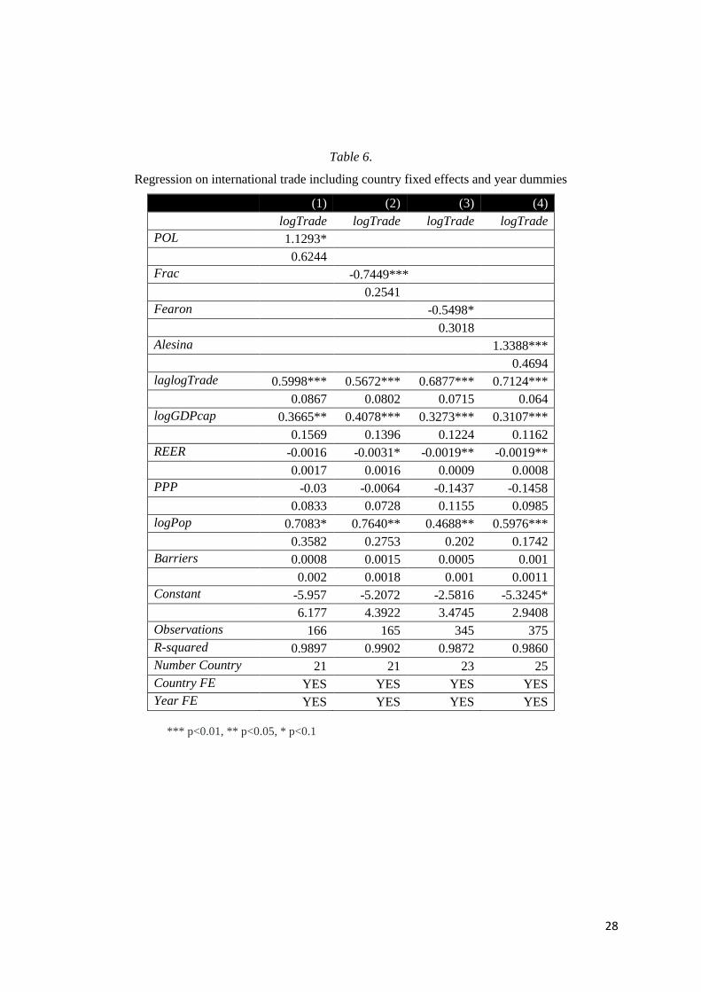
The main model includes country fixed effects and year dummies that simulate the year
fixed effects and the results are shown in table 6. Model 1 to Model 4 are respectively the
regressions with different measures for ethnic diversity, being the polarization and
fractionalization index I created and calculated, and the indexes of Fearon (2003) and Alesina
et al. (2003). It is notable that the signs of the estimates are not unanimous. Even more striking
is the fact that POL and Fearon respectively Frac and Alesina are calculated according to the
same formula and those pairs of indexes show different signs. Only POL and Alesina have the
28
Table 6.
Regression on international trade including country fixed effects and year dummies
(1) (2) (3) (4) logTrade logTrade logTrade logTrade
POL 1.1293*
0.6244
Frac -0.7449***
0.2541
Fearon -0.5498*
0.3018
Alesina 1.3388*** 0.4694
laglogTrade 0.5998*** 0.5672*** 0.6877*** 0.7124*** 0.0867 0.0802 0.0715 0.064
logGDPcap 0.3665** 0.4078*** 0.3273*** 0.3107*** 0.1569 0.1396 0.1224 0.1162
REER -0.0016 -0.0031* -0.0019** -0.0019** 0.0017 0.0016 0.0009 0.0008
PPP -0.03 -0.0064 -0.1437 -0.1458 0.0833 0.0728 0.1155 0.0985
logPop 0.7083* 0.7640** 0.4688** 0.5976*** 0.3582 0.2753 0.202 0.1742
Barriers 0.0008 0.0015 0.0005 0.001 0.002 0.0018 0.001 0.0011
Constant -5.957 -5.2072 -2.5816 -5.3245* 6.177 4.3922 3.4745 2.9408
Observations 166 165 345 375
R-squared 0.9897 0.9902 0.9872 0.9860
Number Country 21 21 23 25
Country FE YES YES YES YES
Year FE YES YES YES YES
*** p<0.01, ** p<0.05, * p<0.1

29
expected sign and are significant, at the 10% respectively 1% level. On the other hand, Frac
and Fearon are negative, indicating that more ethnic diversity is trade deterring, for which
Fearon is significant at the 10% level and Frac at the 1% level. Control variables which are,
besides the lagged value of trade, highly significant, are GDP per capita of a country and the
population, which represent the wealth and size of the economy. Both have positive values
meaning that the wealth and the size of the country, are boosting international trade. Moreover,
REER is, however not always, significant and negative implying that a depreciation of its
currency is trade increasing.
Introducing an interaction term for above median high skilled migration estimates
whether a relatively higher share of high skilled migration accelerates the effect on international
trade. A positive sign indicates that the latter increases the effect on trade more than
proportionally. The results are presented in table 7 in the appendix and show insignificant
results for all models except for the model proxied by the Alesina index, where the effect is
estimated to be negative. This implies that having an above median percentage of at least
tertiary education skilled migrants, deters the effect that ethnic diversity, proxied by the Alesina
index, has on international trade. So, the education level of the migration has either no
accelerated effect on international trade or it is contradicting the hypothesis. However, the
results might be biased as the flow of migrants being relatively high-skilled could not have been
able to find a matching job where they can utilize their superior knowledge.
Next, imports and exports are divided aiming to estimate whether the effect is dominated
by the foreign goods demand channel or because of the market creation effect. The results are
presented in table 8 and they do show striking results. First of all, the sign of the coefficients
are again not unanimous, again Frac and Fearon show a negative coefficient. Regardless of the
sign, the coefficient of ethnic diversity for imports is always higher than for exports and
moreover always significant, whereas it is mostly insignificant for exports. This indicates that
the effect is driven by the demand side of the migrants rather than the fall in transaction costs,
that confors the existing empirical literature. In other words, the foreign goods channel is
dominating the market creation effect. The controls do not show striking results, although the
REER is significant in most cases, but surprisingly both for imports and exports negative. One
would expect the sign to be positive for imports meaning that in case of real exchange rate rise,
the goods are becoming more expensive relative to foreign goods, thus, foreign goods become
relatively cheaper and imports increase.

30
*** p<0.01, ** p<0.05, * p<0.1
Table 8.
Regression on exports and imports separated including country fixed effects and year dummies
(12) (13) (14) (15) (16) (17) (18) (19)
logExport logImport logExport logImport logExport logImport logExport logImport
POL 0.9143 1.1293*
0.6936 0.6244
Frac
-0.559** -0.7449***
0.2565 0.2541
Fearon
0.0885 -0.5498*
0.2438 0.3018
Alesina
0.1897 1.3388***
0.3959 0.4694
laglogExport 0.8470*** 0.8723*** 0.8047*** 0.8301***
0.1012
0.0986
0.0447
0.0422
laglogImport 0.5998*** 0.5672*** 0.6877*** 0.7124***
.0867
0.0802
0.0715
0.064
logGDPcap 0.271 0.3665** 0.282 0.4078*** 0.1904** 0.3273*** 0.1748** 0.3107***
0.1854 0.1569 0.1831 0.1396 0.0793 0.1224 0.0794 0.1162
REER -
0.0028**
-0.0016 -0.0028* -0.0031* -0.001 -0.0019** -0.0011 -0.0019**
0.0011 0.0017 0.0013 0.0016 0.0007 0.0009 0.0007 0.0008
PPP -0.0461 -0.03 -0.0678 -0.0064 -0.1586 -0.1437 -0.1579 -0.1458
0.1073 0.0833 0.1054 0.0728 0.1158 0.1155 0.1076 0.0985
logPop 0.6035 0.7083* 0.7729* 0.7640** 0.1186 0.4688** 0.2593* 0.5976***
0.4986 0.3582 0.4343 0.2753 0.1828 0.202 0.1381 0.1742
Barriers -0.0003 0.0008 -0.0009 0.0015 0.0007 0.0005 0.0013 0.001
0.003 0.002 0.0027 0.0018 0.0007 0.001 0.001 0.0011
Constant -9.0748 -5.957 -11.5471 -5.2072 1.2926 -2.5816 -1.4865 -5.3245*
10.1229 6.177 8.4786 4.3922 3.4036 3.4745 2.5824 2.9408
Observations 166 166 165 165 345 345 375 375
R-squared 0.9886 0.9897 0.9885 0.9902 0.9909 0.9872 0.9897 0.9860
Number of
Country
21 21 21 21 23 23 25 25
Country FE YES YES YES YES YES YES YES YES
Year FE YES YES YES YES YES YES YES YES

31
To conclude, ethnic diversity measured by the polarization index I created and which is
explained thoroughly in this study, is increasing international trade. Ethnic diversity is affecting
international trade dominated by imports over exports, which is due to immigrants demanding
foreign products rather than immigrants possessing superior foreign knowledge or foreign
networks which decrease trade cost and stimulate trade. However, the various measures for
ethnic diversity generate different results. Not only the significance level is disparate but also
the sign of the coefficients which makes it is hard to make conclusions concerning the effects
on international trade. Anyhow, what can be concluded is, that it does matter in which way
ethnic diversity is measured and on beforehand of each study, it should be well elaborated what
measure fits best for the particular study.
Robustness checks The first robustness check is to run regressions including only country fixed effects and for the
random effects model including country dummies only who simulate the country fixed effects.
The results in table 9 in the Appendix show that POL gets insignificant and Frac gets significant
at the 10% level and Fearon at 1%. The signs rises although the controls do not change much
implying that excluding the year dummies, overestimates the results.
The second robustness check is running all models with using the random effect model
including country and year dummies to control for country and year fixed effects. As Fearon
and Alesina cannot be estimated with the fixed effects models, I can now, by using the random
effects models, compare the four models more easily as they are estimated the same way. The
results are shown in table 10 and there are no changes, besides the errors becoming a little bit
smaller.
Continually, table 11 presents the results when correcting for the unit root in the time
series for international trade. POL and Frac do not change much, nonetheless some controls do
not show a significant effect on international trade anymore which is surprising contradicting
the hypothesis. Moreover, both models including the index Fearon and Alesina do not show
predicted significant results. As I have not found any paper taking the first difference of
international trade I neglect these models any further in this study and they only serve as a
robustness check, although not a strong one.
Next, the models are estimated performing first differencing instead of the fixed effect
model. First differencing controls for time invariant unobserved heterogeneity across countries,
by taking the difference of each observation. The results are presented in table 12 and only
Model 1 and Model 2 can be executed using this estimator, as the other models have time

32
invariant variables and would therefore be omitted. The sign of the coefficients do not change,
however, the significance does, POL gets significant at the 5% level and its coefficient
increases. Frac is now only significant at the 10% level and its coefficient becomes more
negative. Overall, it generates no striking changes and therefore the results can concluded to be
robust.
Table 13 shows the output of the model where the depth of cleavage represents only one
of the six dimensions. However none of them are significant, although all staying positive. So,
each dimension itself does not explain a nationality well, it is the combination of dimensions
who can express the characteristics of different nationalities. Moreover, controls who lose their
significance are REER and logPop.
To conclude, the results are robust to changes in the estimation method although not to
changes in the independent variable, measured by the proxy for ethnic diversity or by taking
the first difference to correct for the presence of a unit root.
Causality Two stage least squares (2SLS) is performed to estimate a causal relationship of ethnic diversity
on international trade. The IV estimation is only executed on Model 1 and Model 2 as the other
two proxies are time invariant, and a lagged value would lead to perfect multicollinearity. The
results are presented in table 14 and the instruments lagMigrant respectively lagPOL and
lagFrac represent the percentage of migrant stock the year before respectively the lagged value
of the endogenous variables. Observations drop significantly as compared to OLS regressions
as well as the countries included. Moreover, both instruments generate contradicting results in
both the models and, violate the critical assumption of independence between the error terms
which for both reason makes any conclusion not reliable. However, as causality is an important
issue the table is added to this study to start the discussion of good instruments for ethnic
diversity and to motivate other researches to elaborate on this theme.
10. Limitations In this section, the limitations of this study are mentioned in which the first involves the data.
Almost half of the observations drop because of lack of data especially concerning the foreign
population shares. Even more, some countries were for this reason excluded in the study since
they had no observations for the population shares at all. This reduces the cross sections, which

33
is a loss in precision and, because of the availability of data I was forced to narrow down my
timespan.
Another limitation is the use of aggregated data instead of using bilateral data and
performing a gravity model. Many studies concerning international trade make use of the
gravity model that estimates the relationship using bilateral data, i.e. from a specific country to
another specific country and that for all pairs in the sample. The model includes amongst others
trade, distance, common language, former colony, geography etc. between the two specific
countries and is mostly used aiming to analyze the effect of a change in trade policy. However,
the gravity equation is subject to some critique (Baier & Bergstrand, 2007), and oreover, I am
interested in the total effect of the country its diversity on the total value of trade, instead of
trade with the specific countries where the migrants come from. The more ethnic divers a
country is, the better it is able to cope with more different countries, also as nationals are
familiar with working with other nationalities and because of the other two channels I
mentioned before. Being, first, the foreign products demanded by migrants do not necessarily
need to come from the specific country of origin. Second, migrants do not only possess superior
knowledge about their originating country, as well as also countries similar to that. Therefore,
I would expect total trade to increase and not just trade with that specific country as the various
countries the migrants come from can to some extent be similar to one another.
My data contains only the EU28 countries and therefore variation is minimized as all
countries are incorporated in one union. The EU is characteristic by an internal single market
through a standardized system of laws that apply in all member states. For example, the
emergency procedure following the huge stream of refugees was implemented on EU level.
However, on the other hand, the Schengen agreement makes migration easier within the
participating countries, increasing the variation in ethnic diversity. For a more precise
estimation more countries should be included in the sample that is lacking in this study.
Moreover, an econometrical limitation is the time invariant variables Fearon and
Alesina. Comparisons of the different models are therefore not precise.
Lastly, as already mentioned before, this study incorporates foreign born population,
that does not reveal anything about the employment or level of jobs. This contains information
regarding the ability to utilize their superior knowledge and networks and might have biased
the import versus export conclusion and the accelerated effect education could have.

34
11. Conclusion To conclude, this study aims to estimate the relationship between ethnic diversity on the
aggregate of international trade. The polarization index used as a proxy for ethnic diversity is
international trade enhancing and divides the country in shares based on nationality in which
the depth of cleavage is proxied by the absolute value of the relative difference between the
national culture and the different foreign cultures. That in turn, is measured by the average of
the six cultural dimension of Hofstede. The more divers and diverse cultures live in a country
the more fractionalized the country is, which increases international trade.
The effect is caused by imports rather than exports, in other words, ethnic diversity
affects international trade particularly due to the migrants demanding foreign products rather
than the decrease in trading costs because of the market creation effect. However it should be
noted that the channel through which imports are affected is always present as migrants demand
foreign products. The export channel cannot be exploited when migrants have not found a
matching job where they can utilize their superior knowledge and networks, that is not included
in this study. Also, the accelerated effect of skilled migration on trade could for this reason have
disappeared.
However, ethnic diversity can be measured by different indexes and according to the
correlations between them and the results from the regressions, they do differ greatly and
generate different results. For example, when excluding the depth of cleavage and only
measuring ethnic diversity by the change that two randomly chosen inhabitants of a country
belong to separate groups within society, turns the effect to be trade deterring. Moreover, the
data that is already published about the time invariant measure for ethnic fractionalization from
Alesina et al. (2003) and Fearon (2003) generate dissimilar results. Therefore, before starting a
study it is important to understand the exact aim and which measure for ethnic diversity is most
appropriate to use in each study.
This reserach contributes to the existing literature for making it possible to perform a
panel data regression including fixed effect, when calculating the yearly values for ethnic
diversity instead of time invariant values. Moreover, the effect of ethnic diversity on aggregated
international trade has never been analyzed before. As differences in the measures are present
and correlations are small, further research on the strength of the measures is required to be able
to use the appropriate index for different studies.

35
12. References Alesina, A., & La Ferrara, E. (2005). Ethnic Diversity and Economic Growth. Discussion
Paper, Harvard University.
Alesina, A., & Wacziarg, R. (1998). Openness, country size and government. Journal of
Public Economics 69, 305–321.
Alesina, A., Devleeschauwer,, A., Easterly, W., Kurlat, S., & Wacziarg, R. (2003).
Fractionalization. Journal of Economic growth 8.2, 155-194.
Auboin, M., & Ruta, M. (2013). The relationship between exchange rates and international
trade: a literature review. World Trade Review 12.03 , 577-605.
Baier, S., & Bergstrand, J. (2007). Do free trade agreements actually increase members'
international trade? Journal of international Economics 71.1, 72-95.
CBS. (2017). Gerapporteerde spanningen in de samenleving en eigen ervaringen daarmee.
Bevolkingstrend 2017.
Dickey, D., & Fuller, W. (1979). Distribution of the estimators for autoregressive time series
with a unit root. Journal of the American Statistical Association 74, 427–431.
Docquier, F., & Lodigiani, E. (2010). Skilled migration and business networks. Open
Economies Review 21.4, 565-588.
Dreher, A. (2006). Does globalization affect growth? Evidence from a new index of
globalization. Applied Economics 38, 1091-1110.
Easterly, W., & Levine, R. (1997). Africa's growth tragedy: policies and ethnic divisions. The
Quarterly Journal of Economics 112.4, 1203-1250.
Egger, P., Ehrlich, Von, M., & Nelson, D. (2012). Migration and Trade. The World Economy
35.2, 216-241.
Esteban, J., & Ray, D. (1994). On the Measurement of Polarization. Econometrica 62(4), 819-
851.
Fearon, J. (2003). Ethnic and cultural diversity by country. Journal of Economic Growth 8.2,
195-222.
Garcia-Montalvo, J., & Reynal-Querol, M. (2004). Ethnic polarization, potential conflict, and
civil wars.

36
Genc, M., Gheasi, M., Nijkamp, P., & Poot. (2012). The impact of immigration on
international trade: a meta-analysis. Migration Impact Assessment: New Horizons 301.
Genc, M., Gheasi, M., Nijkamp, P., & Poot, J. (2011). The impact of immigration on
international trade: A meta-analysis.
Girma, S., & Yu, Z. (2002). The link between immigration and trade: Evidence from the
United Kingdom. Weltwirtschaftliches Archiv 138.1, 115-130.
Gould, D. (1994). Immigrant links to the home country: empirical implications for US
bilateral trade flows. The Review of Economics and Statistics, 302-316.
Grimes , J., & Grimes, B. (1996). Ethnologue: Languages of the World, 13 edn : . Dallas, TX:
Summer Institute of Linguistics.
Head, K., & Reis, J. (1998). Immigration and trade creation: econometric evidence from
Canada. Canadian journal of economics, 47-62.
Hering, L., & Paillacar, R. (2015). Does Access to Foreign Markets Shape Internal Migration?
Evidence from Brazil. The World Bank Economic Review 30.1, 78-103.
Hofstede, G. (1983). National cultures in four dimensions: A research-based theory of cultural
differences among nations. International Studies of Management & Organization
13.1-2 , 46-74.
Hofstede, G. (2017, May 23). The six cultural dimensions. Retrieved from Hofstede's cultural
dimensions: http://geerthofstede.com/culture-geert-hofstede-gert-jan-hofstede/6d-
model-of-national-culture/
Jansen, M., & Nordås, H. (2004). Institutions, trade policy and trade flows. Working Paper.
Markusen, J. (1983). Factor movements and commodity trade as complements. Journal of
international economics 14.3-4, Journal of international economics 14.3-4.
McLeod, P., & Lobel, S. (1992). The effects of ethnic diversity on idea generation in small
groups. Academy of Management Proceedings. Vol. 1992. No. 1. Academy of
Management.
Mundell, R. (1957). International trade and factor mobility. The American Economic Review
47.3, 321-335.

37
Mundra, K. (2005). Immigration and international trade: A semiparametric empirical
investigation. The Journal of International Trade & Economic Development 14.1, 65-
91.
Mundra, K. (2005). Immigration and international trade: A semiparametric empirical
investigation. The Journal of International Trade & Economic Development 14.1, 65-
91.
Parsons, C. (2005). Quantifying the trade-migration nexus of the enlarged EU. A comedy or
errors of much ado about nothing.
Peters, M. (2015). Open trade, closed borders Immigration in the era of Globalization. World
Politics 67.01 , 114-154.
Ram, R. (2009). Openness, country size, and government size: Additional evidence from a
large cross-country panel. Journal of Public Economics 93.1 , 213-218.
Samuelson, P. (1948). Samuelson International Trade and the Equalisation of Factor Prices.
Economic Journal, 58, 230,, 163-84.
Wagner, F., Keith, H., & Reis, J. (2002). Immigration and the Trade of Provinces. Scottish
Journal of Political Economy 49.5 , 507-525.
Woolridge, J. (2012). Introductory Econometrics; A Modern Approach. In J. Woolridge,
Introductory Econometrics; A Modern Approach (p. Ch 11). Mason: South-Western,
Cengage Learning.
World Bank. (2017, May). International migrant stock (% of population). Retrieved from
World Bank Indicators: http://data.worldbank.org/indicator/SM.POP.TOTL.ZS
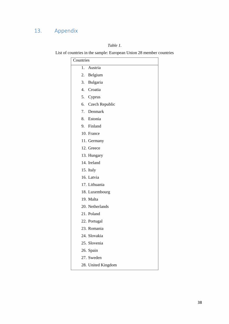
38
13. Appendix
Table 1.
List of countries in the sample: European Union 28 member countries
Countries
1. Austria
2. Belgium
3. Bulgaria
4. Croatia
5. Cyprus
6. Czech Republic
7. Denmark
8. Estonia
9. Finland
10. France
11. Germany
12. Greece
13. Hungary
14. Ireland
15. Italy
16. Latvia
17. Lithuania
18. Luxembourg
19. Malta
20. Netherlands
21. Poland
22. Portugal
23. Romania
24. Slovakia
25. Slovenia
26. Spain
27. Sweden
28. United Kingdom

39
Table 2.
Regions in the world
1. North America
2. South America
3. Central America
4. Caribbean
5. Northern Europe
6. Western Europe
7. Eastern Europe
8. Southern Europe
9. Northern Africa
10. Western Africa
11. Eastern Africa
12. Middle Africa
13. Southern Africa
14. Middle Africa
15. Western Asia
16. Central Asia
17. Southern Asia
18. Eastern Asia
19. Southeastern Asia
20. Oceania
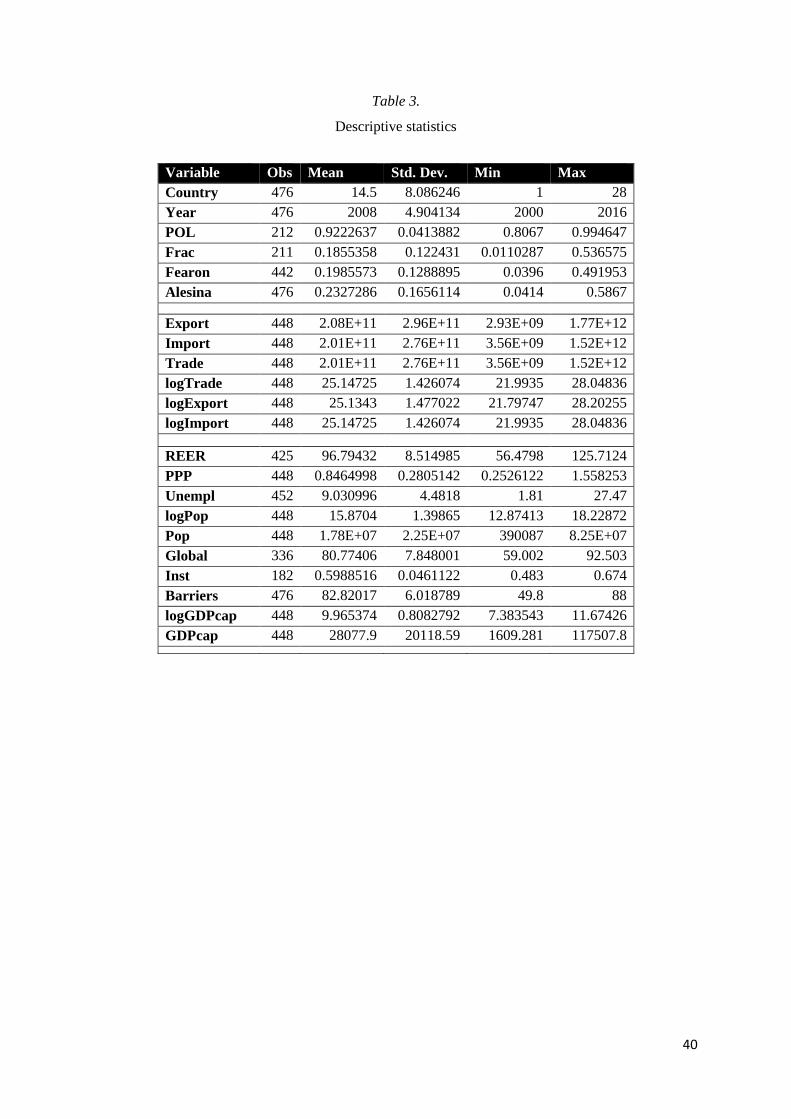
40
Table 3.
Descriptive statistics
Variable Obs Mean Std. Dev. Min Max
Country 476 14.5 8.086246 1 28
Year 476 2008 4.904134 2000 2016
POL 212 0.9222637 0.0413882 0.8067 0.994647
Frac 211 0.1855358 0.122431 0.0110287 0.536575
Fearon 442 0.1985573 0.1288895 0.0396 0.491953
Alesina 476 0.2327286 0.1656114 0.0414 0.5867
Export 448 2.08E+11 2.96E+11 2.93E+09 1.77E+12
Import 448 2.01E+11 2.76E+11 3.56E+09 1.52E+12
Trade 448 2.01E+11 2.76E+11 3.56E+09 1.52E+12
logTrade 448 25.14725 1.426074 21.9935 28.04836
logExport 448 25.1343 1.477022 21.79747 28.20255
logImport 448 25.14725 1.426074 21.9935 28.04836
REER 425 96.79432 8.514985 56.4798 125.7124
PPP 448 0.8464998 0.2805142 0.2526122 1.558253
Unempl 452 9.030996 4.4818 1.81 27.47
logPop 448 15.8704 1.39865 12.87413 18.22872
Pop 448 1.78E+07 2.25E+07 390087 8.25E+07
Global 336 80.77406 7.848001 59.002 92.503
Inst 182 0.5988516 0.0461122 0.483 0.674
Barriers 476 82.82017 6.018789 49.8 88
logGDPcap 448 9.965374 0.8082792 7.383543 11.67426
GDPcap 448 28077.9 20118.59 1609.281 117507.8
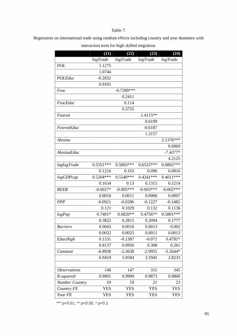
41
Table 7.
Regression on international trade using random effects including country and year dummies with
interaction term for high skilled migration.
(21) (22) (23) (24)
logTrade logTrade logTrade logTrade
POL 1.1275
1.0744
POLEduc -0.2832
0.9101
Frac
-0.7289***
0.2411
FracEduc
0.114
0.3755
Fearon
1.4115**
0.6199
FearonEduc
-0.6187
1.3157
Alesina
2.1376***
0.6969
AlesinaEduc
-7.4377*
4.2125
laglogTrade 0.5551*** 0.5003*** 0.6525*** 0.6802***
0.1216 0.103 0.096 0.0816
logGDPcap 0.5204*** 0.5540*** 0.4241*** 0.4011***
0.1634 0.13 0.1315 0.1214
REER -0.0027* -0.005*** -0.003*** -0.002***
0.0016 0.0011 0.0006 0.0007
PPP -0.0921 -0.0286 -0.1227 -0.1482
0.121 0.1029 0.132 0.1136
logPop 0.7401* 0.6820** 0.4756** 0.5801***
0.3822 0.2815 0.2094 0.1777
Barriers 0.0043 0.0016 0.0013 0.002
0.0032 0.0025 0.0011 0.0013
EducHigh 0.1531 -0.1387 -0.071 0.4781*
0.8137 0.0956 0.308 0.261
Constant -6.8938 -3.3638 -2.9955 -5.2644*
6.9419 5.0584 3.5945 2.8233
Observations 148 147 315 345
R-squared 0.9901 0.9909 0.9873 0.9860
Number Country 19 19 21 23
Country FE YES YES YES YES
Year FE YES YES YES YES
*** p<0.01, ** p<0.05, * p<0.1

42
Table 9.
Regression on international trade including country fixed effects
(1) (2) (3) (4) logTrade logTrade logTrade logTrade
POL 1.193
0.8927
Frac
-0.8440*
0.4807
Fearon
-1.9495***
0.3642
Alesina
4.0041***
0.6435
laglogTrade 0.1753*** 0.1507*** 0.1765*** 0.1867***
0.0459 0.0451 0.0477 0.0475
logGDPcap 1.0623*** 1.0857*** 1.0440*** 1.0276***
0.0985 0.1007 0.1084 0.1094
REER -0.0032 -0.0060** -0.0040** -0.0040**
0.003 0.0027 0.0017 0.0016
PPP -0.0579 -0.011 -0.0881 -0.0745
0.0908 0.0732 0.1193 0.1184
logPop 1.6173*** 1.6267*** 1.1058*** 1.2113***
0.4515 0.4701 0.2927 0.2632
Barriers -0.0005 0.0014 -0.0001 0.0005
0.0038 0.0038 0.0017 0.0017
Constant -16.500** -14.9486* -6.7608 -9.2211**
7.7978 7.3641 4.5776 4.1282
Observations 166 165 345 375
R-squared 0.9621 0.9633 0.9631 0.9636
Number Country 21 21 23 25
Country FE YES YES YES YES
Year FE NO NO NO NO
*** p<0.01, ** p<0.05, * p<0.1

43
Table 10.
Regression on international trade using random effects model including country and year dummies
(20) (21) (3) (4)
logTrade logTrade logTrade logTrade
POL 1.1293*
0.6729
Frac
-0.7449***
0.274
Fearon
-0.5498*
0.3018
Alesina
1.3388***
0.4694
laglogTrade 0.5998*** 0.5672*** 0.6877*** 0.7124***
0.0934 0.0865 0.0715 0.064
logGDPcap 0.3665** 0.4078*** 0.3273*** 0.3107***
0.169 0.1505 0.1224 0.1162
REER -0.0016 -0.0031* -0.0019** -0.0019**
0.0018 0.0017 0.0009 0.0008
PPP -0.03 -0.0064 -0.1437 -0.1458
0.0897 0.0785 0.1155 0.0985
logPop 0.7083* 0.7640** 0.4688** 0.5976***
0.386 0.2968 0.202 0.1742
Barriers 0.0008 0.0015 0.0005 0.001
0.0021 0.0019 0.001 0.0011
Constant -5.8558 -5.0661 -2.5816 -5.3245*
6.5971 4.6878 3.4745 2.9408
Observations 166 165 345 375
R-squared 0.9897 0.9902 0.9872 0.9860
Number of
Country
21 21 23 25
Country FE YES YES YES YES
Year FE YES YES YES YES
*** p<0.01, ** p<0.05, * p<0.1

44
Table 11.
Regression on international trade using fixed effects and year dummies and correcting for the
unit root
(1) (2) (3) (4)
D.logTrade D.logTrade D.logTrade D.logTrade
POL 1.4246*
0.7399
Frac
-0.7162**
0.3344
Fearon
-0.0422
0.3239
Alesina
0.144
0.4175
laglogTrade = D, 0.1115 0.0698 0.2323*** 0.2378***
0.1069 0.1019 0.066 0.0502
logGDPcap 0.1045 0.1125 0.0246 0.0186
0.127 -0.1298 -0.0596 -0.0535
REER -0.0015 0.0029 0.0015 0.0013
-0.0013 -0.002 -0.001 -0.0009
PPP 0.1569* 0.1469* -0.1252 -0.1270*
0.0847 0.0847 0.0776 0.0711
logPop 1.0341** 1.1040** 0.2598 0.2934**
0.4539 0.4651 0.2031 0.1414
Barriers -0.0001 0.0005 0.0004 0.0007
0.0023 0.0021 0.0009 0.001
Constant -18.8245** -18.6183** -4.1087 -4.6367*
8.6952 8.3782 3.6204 2.5962
Observations 158 157 322 350
R-squared 0.9205 0.9217 0.9206 0.9199
Number of
Country
20 20 23 25
Country FE YES YES YES YES
Year FE YES YES YES YES
*** p<0.01, ** p<0.05, * p<0.1

45
Table 12.
Regression on international trade using first differencing
(25) (26)
D.logTrade D.logTrade
POL = D, 1.8819***
0.6496
Frac = D,
-2.6435*
1.4776
logGDPcap = D, 1.1548*** 1.1660***
0.1332 0.1436
REER = D, -0.0102** -0.0099**
0.0047 0.0047
PPP = D, 0.2358 0.2048
0.167 0.1793
logPop = D, 2.3082*** 3.4526**
0.8447 1.3497
Barriers = D, 0.0031* 0.0036*
0.0018 0.0019
Constant 0.0036 0.0058
0.008 0.0075
Observations 137 137
Number of
Country
16 16
FD YES YES
Year FE NO NO
*** p<0.01, ** p<0.05, * p<0.1

46
Table 13.
Regression on international trade including country fixed effects and year dummies using each
dimension separately as a proxy for the depth of cleavage
(6) (7) (8) (9) (10) (11)
logTrade logTrade logTrade logTrade logTrade logTrade
D1 0.0558
0.8335
D2
0.6449
1.0627
D3
-0.3266
1.0904
D4
1.3349
0.9554
D5
2.6823
2.5791
D6
3.1057
2.4268
laglogTrade 0.6022*** 0.5984*** 0.6038*** 0.5979*** 0.5980*** 0.5861***
0.0834 0.0842 0.0814 0.0854 0.0854 0.088
logGDPcap 0.3520** 0.3549** 0.3511** 0.3546** 0.3543** 0.3688**
0.1634 0.1641 0.1626 0.1609 0.1587 0.164
REER -0.0018 -0.0018 -0.0017 -0.0018 -0.0017 -0.0019
0.0019 0.0019 0.0019 0.0019 0.0018 0.0019
PPP -0.0498 -0.0492 -0.0548 -0.0361 -0.0221 -0.0091
0.102 0.1011 0.0985 0.0867 0.0746 0.0736
logPop 0.3915 0.4324 0.364 0.4843 0.5552 0.5959
0.3464 0.3384 0.3547 0.4136 0.3956 0.3856
Barriers 0.001 0.0011 0.0009 0.0014 0.0013 0.0015
0.002 0.0019 0.0019 0.0018 0.0018 0.0018
Constant 0.3115 -0.2715 0.7279 -1.113 -2.2544 -2.7525
5.532 5.3633 5.6652 6.5128 6.1949 6.03
Observations 166 166 166 166 166 166
R-squared 0.9894 0.9894 0.9894 0.9894 0.9895 0.9896
Number
Country
21 21 21 21 21 21
Country FE YES YES YES YES YES YES
Year FE YES YES YES YES YES YES
*** p<0.01, ** p<0.05, * p<0.1

47
Table 14.
Regression on international trade using 2SLS with instruments for the explanatory variables POL and
Frac
(25) (26) (27) (28) logTrade logTrade logTrade logTrade
Instruments lagMigrant lagPOL lagMigrant lagFrac
POL 6.7932** 16.426
30.176 11.388
Frac
-13.546 -0.9690**
25.9177 0.4646
logGDPcap 0.6515*** 0.5786*** 0.6579 0.5607***
0.1457 0.0869 0.4376 0.0837
REER 0.0001 -0.0053*** -0.0304 -0.0046***
0.0015 0.0014 0.0393 0.0015
PPP 0.2133 -0.0028 14.814 -0.0430
0.2424 0.1122 21.147 0.1122
logPop 3.0097*** 0.7283* 41.199 0.8805**
0.9018 0.4137 40.350 0.3843
Barriers -0.0062 0.0050 0.0299 0.0035
0.0041 0.0034 0.0485 0.0034
Constant -43.887** -38.517 -469.174 -50.054
171.340 82.852 553.655 70.392
Observations 80 137 79 137
Number of
Country
15 16 15 16
Country FE YES YES YES YES
Year FE YES YES YES YES
*** p<0.01, ** p<0.05, * p<0.1