ethanol chemical vapor deposition process design for ...1489/... · ethanol chemical vapor...
TRANSCRIPT

Ethanol Chemical Vapor Deposition Process Design for Selective
Growth of Vertically-Aligned Single-Walled Carbon Nanotubes
A Dissertation Presented
by
Hatem Mansour Abuhimd
to
The Department of Mechanical and Industrial Engineering
in partial fulfillment of the requirements
for the degree of
Doctor of Philosophy
in the field of
Industrial Engineering
Northeastern University
Boston, Massachusetts
December 2011

ii
Abstract
Science and engineering communities have given the synthesis of vertically
aligned single walled carbon nanotubes (VA-SWNTs) considerable attention
due to their attractive physical properties, unique morphology, and better
potential for building advanced devices than those with asymmetric and
entwined carbon nanotubes (CNTs). Chemical vapor deposition (CVD) is one of
several viable methods for growing VA-SWNTs, which is well known for its
economic viability and good yield of VA-SWNTs. Utilizing Co catalyst (0.5 ~ 1
nm thick) supported on an Al/SiO2 multilayer substrate and a hydrocarbon
feedstock, VA-SWNTs are grown in excess of a millimeter height.
To control the CVD process to selectively produce tall VA-SWNTs, one has to
use the right combination of process inputs such as gas flow rate, chamber
temperature, and chamber pressure. This dissertation investigates their main
effects and interactions on VA-SWNT yield and length by conducting design of
experiments and analysis on the metamodel of the CVD process. The artificial

iii
neural network (ANN) based metamodel was constructed using the
experimental data.
The interactions among control variables and response surface plots show that
pressure and temperature are the most significant CVD process control
variables to selectively produce VA-SWNTs. In addition, the analysis confirms
that higher temperature and higher pressure will result in a better yield of VA-
SWNTs. In contrast, the analysis points out that the flow rate and the pressure
are the most statistically significant factors that influence the length of VA-
SWNTs. The response surface graphs indicate that higher flow with lower
pressure will consistently yield tall VA-SWNTs. We found that gas flow rate is
the most significant of the control variables and only the optimum value of the
gas flow rate can ensure the growth of tall VA-SWNTs. We also found that the
interaction of gas flow rate with chamber temperature and pressure is
extremely important to ensure the quality of VA-SWNTs. This observation
indicates that dynamic pressure of the fluid in the chamber affects the quality of
VA-SWNTs grown on the substrate. We have also found out that flow rate less
than 150 sccm and a growth time of 20 minutes are suitable for the repeatability

iv
of medium length VA-SWNTs. Outcomes of this investigation are beneficial for
moving the CVD process closer to producing VA-SWNTs on large mass-
produced scale.

v
Table of Contents
Abstract ............................................................................................................................. ii
List of Figures .............................................................................................................. viii
List of Tables ................................................................................................................ xiii
1. Introduction ......................................................................................................... 1
2. Literature Review ................................................................................................ 7
2.1 Vertically Aligned Single Walled Carbon Nanotubes .................................................. 7
2.1.1 Experimental Methods ................................................................................. 10
2.1.2 Growth Mechanism ...................................................................................... 16
2.1.3 Applications ................................................................................................. 20
2.2 Computational Methods .............................................................................................. 22
2.2.1 Multi-Layer Perceptron ................................................................................ 23
2.2.2 Design of Experiments ................................................................................. 24
2.3 Design of Experiments for CVD Grown Carbon Nanotubes...................................... 26
2.3.1 Experiments and Discussion ........................................................................ 34
3. Experimental Setup .......................................................................................... 40

vi
3.1 System Variables ........................................................................................................ 42
3.2 Catalyst Preparation .................................................................................................... 45
3.3 CVD Process Setup ..................................................................................................... 45
4. Process Design for Controllability ................................................................ 47
4.1 Metamodel and Design of Experiments ...................................................................... 48
4.2 Comparison of Main Effects Plots .............................................................................. 52
4.3 Pareto and General Response Surface Plots ............................................................... 54
5. Process Design for Length Assurance ........................................................... 56
5.1 Metamodel and Design of Experiments ...................................................................... 57
5.2 Pareto Chart Analysis ................................................................................................. 65
5.3 Marginal Mean Plots ................................................................................................... 66
5.4 Comparison of Main Effects Plots .............................................................................. 67
5.5 General Response Surface Plot ................................................................................... 69
6. Process Design for CVD Flow ........................................................................ 73
6.1 Pareto Chart Analysis ................................................................................................. 77
6.2 Comparison of Main Effects Plots .............................................................................. 78

vii
6.3 General Response Surface Plot ................................................................................... 79
7. Scientific Formulation of the Process Input Variables .............................. 80
7.1 Ideal Gas Law ............................................................................................................. 83
7.2 Dynamic Pressure ....................................................................................................... 85
8. Conclusion and Future Work.......................................................................... 88
References ....................................................................................................................... 90
Appendix A .................................................................................................................... 99
Appendix B ................................................................................................................... 102
Appendix C .................................................................................................................. 139
Appendix D .................................................................................................................. 155
Appendix E ................................................................................................................... 159

viii
List of Figures
Figure 1.1 CVD of VA-SWNTs input output diagram (Co: Cobalt, C: Carbon) ..... 2
Figure 1.2 Schematic of the modeling process framework ........................................ 4
Figure 2.1 Homogenous MWNT samples in a network characterized by TEM
done by Iijima in 1991 [6] ................................................................................................ 8
Figure 2.2 Schematic of the types of pure Carbon forms like Carbon Nanotubes,
Graphite and Diamond [7] .............................................................................................. 9
Figure 2.3 Schematic of the arc-discharge apparatus employed for CNT
production [12] ............................................................................................................... 11
Figure 2.4 Laser ablation schematic for growing CNTs [12] ................................... 12
Figure 2.5 Schematics of ethanol CVD systems and experimental procedures for
the growth of VA-SWNTs ............................................................................................. 13
Figure 2.6 (a) An image of the 2.5-mm-height VA-SWNTS (b) & (c) SEM images
of VA-SWNTs [6] ........................................................................................................... 16

ix
Figure 2.7 CVD grown VA-SWNTS base or tip growth mechanism schematic
with catalyst as Cobalt................................................................................................... 19
Figure 2.8 Scanning electron microscope image of a VA-CNTs membrane (scale
bar = 10 μm) [18] ............................................................................................................. 20
Figure 2.9 Histogram of observed permeability in VA-CNTs [18] ......................... 21
Figure 2.10 5 mm long TiO2/CNT arrays [20] ............................................................ 22
Figure 2.11 Architecture of a Multilayer Perceptron ................................................ 24
Figure 2.12 Most researchers utilize Full Factorial designs for their publications
instead of other techniques like Fractional Factorial and Taguchi ......................... 32
Figure 2.13 Histogram of years 2004-2009 of papers related to Orthogonal
Arrays .............................................................................................................................. 33
Figure 2.14 Schematic diagram of the CCVD setup for carbon nanotube
synthesis .......................................................................................................................... 35
Figure 2.15 Schematic diagram of VCVD [50] ........................................................... 36

x
Figure 3.1 Schematics of ethanol CVD systems and experimental procedures for
the growth of VASWMTs ............................................................................................. 41
Figure 3.2 Cause and effect matrix of input variables .............................................. 44
Figure 3.3 Schematic of the cross section of the substrate ........................................ 45
Figure 4.1 Classifications accuracy of process outcome ........................................... 51
Figure 4.2 Interaction Plots between Temperature and Pressure for VA-SWNTS53
Figure 4.3 Process Analysis Pareto Plot ...................................................................... 55
Figure 4.4 Response Surface Plots of VA-SWNTs Length (Temperature VS
Pressure) .......................................................................................................................... 55
Figure 5.1 Architecture of a multi-layer perceptron network ................................. 59
Figure 5.2 VA-SWNTs length (target) versus estimated VA-SWNTs length
(output) regressions graph for the MLP 4-21-1 network ......................................... 60
Figure 5.3 Histograms showing the distribution of control variables in the
training data for neural networks ................................................................................ 64

xi
Figure 5.4 Process Pareto Analysis, (A) CVD Temperature (°C), (B) CVD
Pressure (sccm), (C) Gas Flow Rate (Torr) ................................................................. 65
Figure 5.5 Marginal mean plots, (A) CVD Temperature (°C), (B) CVD Pressure
(sccm), (C) Gas Flow Rate (Torr) .................................................................................. 66
Figure 5.6 Main effect plots for VA-SWNTs length of pressure and flow ............. 68
Figure 5.7 Response surface plot of VA-SWNTs length VS flow rate VS pressure 70
Figure 5.8 Main effect plots for VA-SWNTs length of temperature and flow ...... 71
Figure 5.9 Response surface plot of VA-SWNTs length VS flow rate VS
temperature ..................................................................................................................... 72
Figure 6.1 VA-SWNTs length (target) versus estimated VA-SWNTs length
(output) regressions graph for the MLP 2-12-1 network ......................................... 74
Figure 6.2 Process Pareto analysis .............................................................................. 77
Figure 6.3 Main effect plots for VA-SWNTs length of time and flow .................... 78
Figure 6.4 Response surface plot of VA-SWNTs length VS flow rate VS time ..... 79

xii
Figure 7.1 First and second runs graphs to measure the stability of pressure
sensor during VA-SWNTs growth time (average = 705.2 torr, 703.5 torr) ............ 81
Figure 7.2 Matrix plots between flow, temperature and pressure for VA-SWNTS
(101 = VA-SWNTs, 102 = MWNTs, 103 = MWNTs & SWNTs, 104 = None) .......... 84
Figure 7.3 Interaction plots between temperature and pressure for VA-SWNTs 86

xiii
List of Tables
Table 2.1 Historical timeline of CNT growth methods [19] .................................... 14
Table 2.2 Researchers used many substrate materials to produce the tubes [19] . 17
Table 2.3 The feasible factorial design either for full or fractional factorial
designs, which can be utilized to optimize processes .............................................. 25
Table 2.4 Taguchi Designs orthogonal arrays ............................................................ 26
Table 2.5 Journals including nanotechnology papers utilizing DOE ..................... 27
Table 2.6 Publications using variable conventional processes and designs for the
optimization of carbon nanotubes characteristic [23-26,31,32,34,38,45-49] ........... 28
Table 2.7 Nano-manufacturing improvements techniques ..................................... 31
Table 2.8 Summary of articles in the use of Orthogonal Arrays to optimize the
processes and designs related to carbon nanotubes [30,39,41,44,51] ..................... 33
xiv
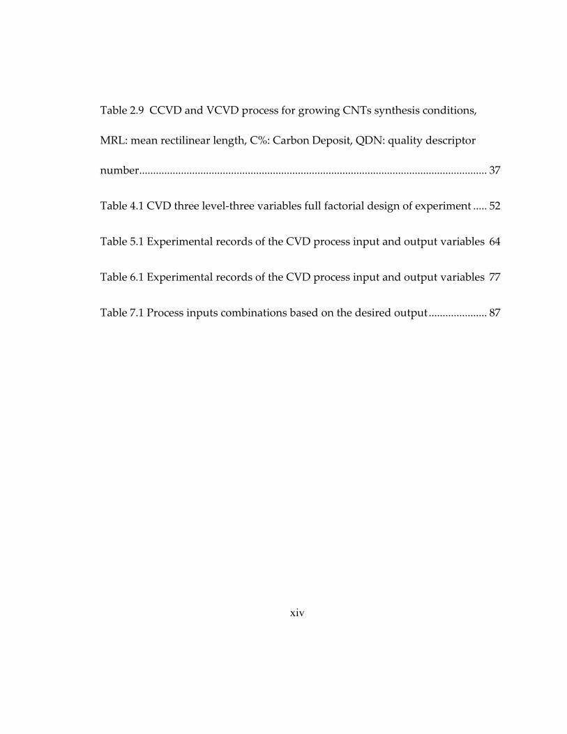
Table 2.9 CCVD and VCVD process for growing CNTs synthesis conditions,
MRL: mean rectilinear length, C%: Carbon Deposit, QDN: quality descriptor
number............................................................................................................................. 37
Table 4.1 CVD three level-three variables full factorial design of experiment ..... 52
Table 5.1 Experimental records of the CVD process input and output variables 64
Table 6.1 Experimental records of the CVD process input and output variables 77
Table 7.1 Process inputs combinations based on the desired output ..................... 87

xv
Acknowledgment
I would like to extend a deep gratitude to my advisors, Prof. Kamarthi and
Prof. Zeid, as they have been the driving force behind my academic and
research success. In addition to their expertise in my research field, I appreciate
their constant encouragement and guidance, which was critical to my
dissertation. I would also like to thank the other member of my committee,
Prof. Jung, for taking the time to understand my work and providing the
feedback. In addition, I would like to acknowledge Prof. Jung’s research group
in general and specifically Dr. Hahm, and Mr. Sanghyun for performing the
experiments. I want to show appreciation to everyone in Network/Nano
Science and Engineering Laboratory and Mechanical and Industrial
Engineering Department and for all their support. I would like to thank my
parents and siblings for instilling in me the seeds of interest and determination
that led me to this career choice, and my lovely wife and two wonderful
daughters for being extremely patient and making the process worthwhile.
Finally, I would like to take this opportunity, to personally, thank everyone
who has assisted, in any way, me in getting my PhD degree.

xvi
Dedication
I dedicate this work to my parents, family, and friends.

1
1. Introduction
Materials at the nanoscale exhibit unparalleled physical and chemical
characteristics in contrast to the macro scale because of the Quantum
phenomena [1]. In addition, mass-producing those materials
(nanomanufacturing) does not receive as much funding as dedicated to their
science [2]. Chemical vapor deposition (CVD) is a common nanomanufacturing
process for growing vertically aligned single walled carbon nanotubes (VA-
SWNTs). It is expected to enable the scale-up of CNT production. However, the
fact that CVD yields only a small fraction of VA-SWNTs makes it hard to scale
up production [3]. To move nanoscience from labs to mass production, a
multidisciplinary scientific approach is needed.
Our proposed approach aims to analyze experimental data from a CVD
process, build neural network models, and perform an experimental design
analysis with the goal of relating the CVD input parameters to the
characteristics of the VA-SWNTs to gain better understanding of their
properties. There are many variables influencing the CVD process; some of
those variables include catalyst type, particle size, surface roughness, reactant

2
composition, etchant composition, reactant pretreatment, and gas flow rate.
Our objective is to evaluate all input variables statistically to find the significant
ones. Figure 1.1 shows the input output diagram for VA-SWNTs growth using
CVD process.
Figure 1.1 CVD of VA-SWNTs input output diagram (Co: Cobalt, C: Carbon)
The figure shows the controllable variables (process inputs), and the key
performance indicators (process outputs). Superior morphology and fascinating

3
physical features of VA-SWNTs can result in interesting applications.
Therefore, we need to address the control of their growth and length. Growing
VA-SWNTs on a substrate surface is an important step toward manufacturing
nanoscale devices [4].. Here are the main objectives of this dissertation
1. Build a deep understanding of CVD based VA-SWNTs growth processes
2. Screen available optimization methods to identify suitable designs
3. Employ the most suitable design
4. Analyze the design results and make recommendations
To achieve the above objectives we plan to analyze a data set from a CVD
machine and perform statistical analysis. In order to relate the CVD input
parameters to the characteristics of the VA-SWNTs, we correlate the input to
the output to allow the optimization and control the CVD process to gain better
VA-SWNTs properties. Figure 1.2 shows the framework flow of the modeling
process.

4
Figure 1.2 Schematic of the modeling process framework
The data analysis for this dissertation is driven by a null hypothesis based on
current publications literature review. The review is related to the CVD grown
VA-SWNTs synthesis process and growth mechanism. For that purpose, the
CVD is presumed to be controllable by researchers to improve the yield. The
expectation is that an understanding of the process controllable variables will
be developed with performing the examination and analyzing the data. That
will result in better designs to control the whole growth process. This
dissertation research was created based upon certain assumptions. Input
5
variables are independent and will yield statistical significant results. Without
such assumption the experimental design results will be hindered and obsolete.
All the efforts are forced to obtain the best quantitative and qualitative data for
the analytical model. Similar assumptions will be applied to the data analysis.
This dissertation will add to the understanding of the VA-SWNTs fabrication
Process, however, certain limitations to the study exist. The data were collected
using traditional sampling methods, which only assess data perceptions of the
independent and dependent variables at one point in time.
The analysis of the CVD grown CNTs process was reported in the literature
before but not for the current process under study. Hence, all variables have to
be considered without the benefit of previous recommendations from old
experiments. The dissertation will examine a metamodel of the CVD VA-
SWNTs synthesis process. The Purpose of the Study is to improve the current
understanding of the VA-SWNTs yield controllability and length. The study
significance iies in the results of such purposes achieved in using such VA-
SWNTs in nanomanufacturing.
The dissertation content is organized as follows. Chapter 2 will go over the
properties and growth mechanism of VA-SWNTs. In addition, it will also

6
describe their importance toward the advancement of nanotechnology.
Moreover, a brief introduction to experimental designs is described including
design of experiment for (Full/Fractional Factorial Designs, Taguchi), Artificial
Neural Networks, and some instances where CNT growth was enhanced by an
experimental design. The method for VA-SWNTS growth and catalyst
preparation with small illustration of the characterization method are discussed
in Chapter 3. Chapter 4 discusses the VA-SWNTs controllability by a
metamodel of an ANN phase and an Experimental Design phase. Chapter 5
will start by an analysis of the VA-SWNTs length assurance experiments results
followed by a general analysis using a similar to chapter 4 metamodel. CVD gas
flow rate relation with the growth time will be analyzed in chapter 6. In chapter
7, we will detail some scientific formulation of the previous metamodels.
Finally, Chapter 8 will present the conclusion and touch on the future research
directions.

7
2. Literature Review
This chapter will give a background on VA-SWNTs and Computational
methods related to this dissertation. The VA-SWNTs section is related to their
remarkable properties and how they were discovered. Then, an illustration of
how they are grown with CVD, growth mechanism and possible future
applications. Here, Computational methods are discussed and related to the
research proposed metamodel. Specifically Artificial neural networks and
design of experiments will be introduced.
2.1 Vertically Aligned Single Walled Carbon Nanotubes
Iijima et al. used arc discharge method to discover CNTs in 1991 (see Figure 2.1)
and it fueled the research about those tubes [5]. Superior morphology and
fascinating physical features of vertically aligned single walled carbon
nanotubes (VA-SWNTs) can result in interesting applications. Therefore, we
need to address the control of their structural growth and organization.
Growing VA-SWNTs on a substrate surface is an important step toward
manufacturing nanoscale devices like field emission displays [4].

8
Figure 2.1 Homogenous MWNT samples in a network characterized by TEM
done by Iijima in 1991 [6]
In general, they bears higher physical quality than other nanoscale carbon
materials [4]. Furthermore, their astonishing purity of 99.98% in a sample
present them as being the purest and highest quality of carbon nanotubes [6].
Their ratio of SWNT to catalyst weight exceeds 50,000% to the other processes
[6]. We can define Multi Walled Carbon Nanotubes (MWNTs) as multiple
rolled concentric tubes of graphite while Single Walled Carbon Nanotubes
(SWNTs) has only one tube [1]. Carbon comes in different molecular structure
like diamond and graphite (Figure 2.2).

9
Figure 2.2 Schematic of the types of pure Carbon forms like Carbon
Nanotubes, Graphite and Diamond [7]
CNT science is a well-researched topic in literature especially for Multi Walled
Carbon Nanotubes (MWNTs)[7]. However, manufacturing those tubes at a
large scale is still an emerging research area [8]. Hence, several researchers are
investigating the large-scale production of CNTs [9]. Our research considers the
nanomanufacturing of VA-SWNTs at a mass production scale. Current methods
for producing VA-SWNTs by CVD have high quality and yield in comparison
to other methods like arc discharge and laser ablation.

10
The task to review VA-SWNTs in literature is made challenging by several
issues. Mainly, there is huge variability of carbon nanotubes. In addition, there
is large amount of published literature researching their physical properties as
pure or compound materials. That literature is produced over a long period and
is generated under very different environments. Therefore, most probably it
discusses very different experimental conditions. Those reasons have driven us
to focus our analysis on more recent work, assuming that older studies are
made obsolete by the new ones.
2.1.1 Experimental Methods
There are three major ways to grow CNTs (SWNT, MWNTs, VA-SWNTs):
electric arc discharge, laser ablation, and chemical vapor deposition (CVD). Arc
discharge was the method used to discover CNT in 1991 by Iijima [5]. Here is a
brief discussion about those main techniques and their characteristics.
Electric Arc Discharge
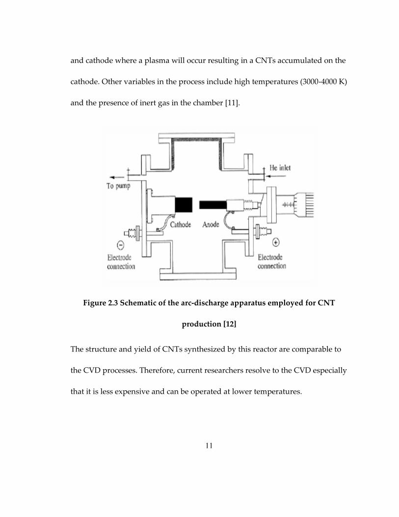
In 1991 Iijima discovered MWNT by the Electric Arc Discharge process [10].
Figure 2.3 shows a drawing of the arc discharge machine [11]. The anode and
cathode are made of graphite. It works by flowing electricity between the anode
11
and cathode where a plasma will occur resulting in a CNTs accumulated on the
cathode. Other variables in the process include high temperatures (3000-4000 K)
and the presence of inert gas in the chamber [11].
Figure 2.3 Schematic of the arc-discharge apparatus employed for CNT
production [12]
The structure and yield of CNTs synthesized by this reactor are comparable to
the CVD processes. Therefore, current researchers resolve to the CVD especially
that it is less expensive and can be operated at lower temperatures.

12
Laser Ablation Method
An alternative to using electric arc discharge is laser ablation. As shown in
Figure 2.4 it utilizes high-energy lasers in high temperature furnaces [11]. The
laser will be used to vaporize metallically catalyzed graphite in the presence of
high temperatures. Similar to the previous process this process is less usable
than the CVD especially that lasers are very costly.
Figure 2.4 Laser ablation schematic for growing CNTs [12]
Chemical Vapor Deposition
In the CVD furnace, a carbonaceous gas is flown over a metallic catalyst. The
carbon under pressure will react with the catalyst and start growing to form the

13
CNT (Figure 2.5) [7]. In contrast, to the previous methods the CVD factors
involved are of moderate ranges. Consequently, the viability of the process for
high yield is promising especially if more research is done in the area. Current
methods for producing CNT by CVD have high quality and yield in
comparison to other methods.
Figure 2.5 Schematics of ethanol CVD systems and experimental procedures
for the growth of VA-SWNTs
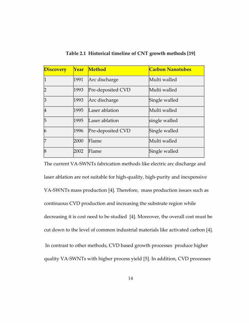
Historically, the research and discoveries in CNTs were happening in rapid
pace (Table 2.1) [12]. CNTs researchers come from different fields with different
scientific background [5]. Such criteria enabled the development of different
techniques and different materials to be utilized.
14
Table 2.1 Historical timeline of CNT growth methods [19]
Discovery Year Method Carbon Nanotubes
1 1991 Arc discharge Multi walled
2 1993 Pre-deposited CVD Multi walled
3 1993 Arc discharge Single walled
4 1995 Laser ablation Multi walled
5 1995 Laser ablation single walled
6 1996 Pre-deposited CVD Single walled
7 2000 Flame Multi walled
8 2002 Flame Single walled
The current VA-SWNTs fabrication methods like electric arc discharge and
laser ablation are not suitable for high-quality, high-purity and inexpensive
VA-SWNTs mass production [4]. Therefore, mass production issues such as
continuous CVD production and increasing the substrate region while
decreasing it is cost need to be studied [4]. Moreover, the overall cost must be
cut down to the level of common industrial materials like activated carbon [4].
In contrast to other methods, CVD based growth processes produce higher
quality VA-SWNTs with higher process yield [5]. In addition, CVD processes

15
require process variables such as temperature and pressure in moderate ranges,
reflecting its potential as cost effective manufacturing technique[13].
In 1996, multi-walled Carbon nanotubes were first aligned utilizing a CVD
process [14]. However, researchers could not grow VA-SWNTs until Murakami
et al. demonstrated their growth in 2004 [15] which were short ~1.5 μm and not
suitable for manufacturing devices. Later, Hata et al. used the assistance of
water to grow VA-SWNTs to 2500 μm [6]. The addition of water prolonged the
catalyst lifetime resulting in taller tubes [6].
The majority of SWNTs grown by CVD use a flow of a gaseous carbon
feedstock over catalyst nanoparticles at medium to high temperature, which
reacts with the catalyst nanoparticles [7]. During CVD growth, VA-SWNTs self-
assemble into vertical structures on the patterned substrate at the catalyst
locations [4,16]. They self-orient and grow perpendicular to the substrate
because of the of van der Waals forces rigidity [7].
Researchers have already mastered the alignment of multiwall carbon
nanotubes while VA-SWNTs alignment understanding is still a challenging task
[17]. Multiple researchers have studied their growth conditions and found that
uncontaminated CVD chamber, gas flow rate and water addition are important

16
control factors and that the vertical or parallel alignment of SWNTs depends
largely on the density of catalyst particles and their distribution in the substrate
[17].
2.1.2 Growth Mechanism
Forming CNT on a substrate surface is an important step toward
manufacturing nanoscale devices. For instance, the vertical forming of CNTs is
particularly essential for field emission displays. The rigidity of MWNT made
them easier for alignment than the flexible SWNT. That VA-SWNTS has higher
quality than other materials.
Figure 2.6 (a) An image of the 2.5-mm-height VA-SWNTS (b) & (c) SEM
images of VA-SWNTs [6]
17
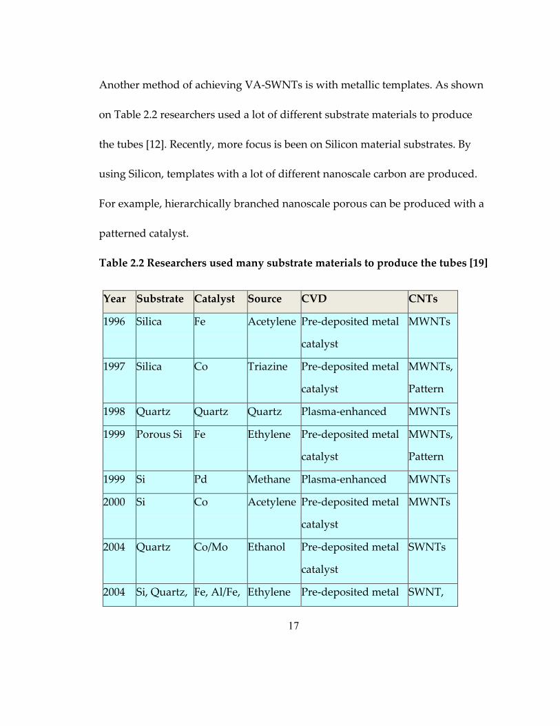
Another method of achieving VA-SWNTs is with metallic templates. As shown
on Table 2.2 researchers used a lot of different substrate materials to produce
the tubes [12]. Recently, more focus is been on Silicon material substrates. By
using Silicon, templates with a lot of different nanoscale carbon are produced.
For example, hierarchically branched nanoscale porous can be produced with a
patterned catalyst.
Table 2.2 Researchers used many substrate materials to produce the tubes [19]
Year Substrate Catalyst Source CVD CNTs
1996 Silica Fe Acetylene Pre-deposited metal
catalyst
MWNTs
1997 Silica Co Triazine Pre-deposited metal
catalyst
MWNTs,
Pattern
1998 Quartz Quartz Quartz Plasma-enhanced MWNTs
1999 Porous Si Fe Ethylene Pre-deposited metal
catalyst
MWNTs,
Pattern
1999 Si Pd Methane Plasma-enhanced MWNTs
2000 Si Co Acetylene Pre-deposited metal
catalyst
MWNTs
2004 Quartz Co/Mo Ethanol Pre-deposited metal
catalyst
SWNTs
2004 Si, Quartz, Fe, Al/Fe, Ethylene Pre-deposited metal SWNT,

18
Metal Foil Al2O3/Fe
Al2O3/Co
catalyst Pattern
2005 Si Al2O3/Fe/
Al2O3
Methane Plasma-enhanced SWNTs
There are four main assumptions about SWNTs growth mechanism [7]. First, a
carbon feedstock and active transition metal nanoparticles are necessary for
their growth unless high temperature is used to heat graphitic carbon
nanoparticles. Second, their diameter is set from the onset of the nanotubes
growth and only a small change will happen if there is a defect. Third, both the
catalyst nanoparticle and the SWNT have the same size (diameter). Fourth, one
catalyst nanoparticle will result in only one nanotube unless the diameters are
different.
There are two types of CNTs diffusion on the substrate, surface or bulk carbon
diffusion [7]. Surface diffusion is related to substrate growth where catalyst
nanoparticles are deposited on a substrate such as SiO2 [7]. The carbon cracks
and nucleates around the solid catalyst and start growing SWNT [7]. Bulk
diffusion can be called a gas phase growth because the formation of catalyst
and nanotube occur in the air [7]. Here the metal nanoparticle dissolve the
cracked carbon until saturation and the growth starts [7]. The growth continues

19
on both types until the carbon source is stopped or the particle is fully coated
with amorphous or graphitic carbon [7].
VA-SWNTs grows either from the catalyst base or from tip and its growth type
depends on the position and size of the catalyst particles (See Figure 2.7) [7].
Thus, the particles detach from the surface of the support material and move at
the tip of growing CNTs for tip-growth. The base growth happens when
nanoscale particles remain attached to the supporting material and CNTs grow
upwards from those metal particles. Figure 2.7 shows both CNTs growth
mechanism.
Figure 2.7 CVD grown VA-SWNTS base or tip growth mechanism schematic
with catalyst as Cobalt

20
2.1.3 Applications
Remarkable applications may result from VA-SWNTs superior morphology
and fascinating physical features. Transport processes for gas and liquid
through CNTs are subjects of deep theoretical and experimental research. One
study uses VACNTs to make gas and liquid membranes [18]. Figure 2.8 shows
a Scanning electron microscope image of that membrane.
Figure 2.8 Scanning electron microscope image of a VA-CNTs membrane
(scale bar = 10 μm) [18]
The VA-CNTs hydrophobic graphitic walls, and nanoscale internal diameters
give rise to an exceptional physical process of ultra-efficient water and gas

21
transport [19]. Water and gas molecules move through nanotube pores 20 or 30
times faster than through other pores of comparable size (see Figure 2.9).
Hence, they will aspire future applications for water desalination, water
purification, nanofiltration, and gas separation.
Figure 2.9 Histogram of observed permeability in VA-CNTs [18]
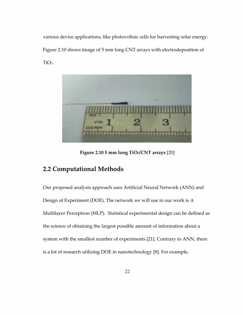
Another application is made from an array of 5 mm aligned titanium oxide/
vertically aligned carbon nanotube (TiO2/CNT) [20]. It was prepared by
electrochemically coating the CNTs with a uniform layer of TiO2 nanoparticles
[20]. The resultant arrays exhibit minimized recombination of photo induced
electron–hole pairs and fast electron transfer from the aligned TiO2/CNT arrays
to external circuits [20]. This enables the assembly of TiO2/CNT arrays for
22
various device applications, like photovoltaic cells for harvesting solar energy.
Figure 2.10 shows image of 5 mm long CNT arrays with electrodeposition of
TiO2.
Figure 2.10 5 mm long TiO2/CNT arrays [20]
2.2 Computational Methods
Our proposed analysis approach uses Artificial Neural Network (ANN) and
Design of Experiment (DOE). The network we will use in our work is A
Multilayer Perceptron (MLP). Statistical experimental design can be defined as
the science of obtaining the largest possible amount of information about a
system with the smallest number of experiments [21]. Contrary to ANN, there
is a lot of research utilizing DOE in nanotechnology [8]. For example,

23
researchers used full and fractional factorial designs to optimize SWNTs [22-
25].
2.2.1 Multi-Layer Perceptron
MLPs are an important class of highly connected feed-forward neural networks
(Figure 2.10). Typically, an MLP consists of a layer of input nodes, one or more
layers of hidden neurons, and a layer of output nodes. The input signal
propagates forward layer by layer with every neuron in the layers representing
a smooth and differentiable nonlinear activation function. The hidden neurons
help the network learn complex features of the relation between input patterns
and outputs. MLPs use a popular supervised learning algorithm named back
propagation, which works in two phases [26].

24
Figure 2.11 Architecture of a Multilayer Perceptron
2.2.2 Design of Experiments
DOE was first used first used in agriculture and has been for over 70 years.
Before information technology DOE was a hard job which requires a skilled
statistician with a wholesome physical knowledge of the process under study to
make an inference about the process [8].
In DOE, factors are the controllable parameters of the process, which have
different levels usually determined by scientific method or experience. Barker et
al. illustrated all of the possible factorial designs in Table 2.3 where the columns

25
are number of factors , rows are number of runs, and III, IV etc. is the fractional
factorial designs [27].
Table 2.3 The feasible factorial design either for full or fractional factorial
designs, which can be utilized to optimize processes
Now we can design the experiment in less time and even analyze the output
with vast speed. Toward this end, choosing a design is the first step, which
requires an understanding of the process input and output. The most used
designs are full and fractional factorial design with high and low levels (two
levels). Other designs like Box–Behnken Design (BBD) are more geared toward
studying the curvature of the design after optimality to deeper understanding

26
of the variables interaction. Another technique is the Taguchi methodology
where the researcher chooses an array and optimizes the process based on it, as
mentioned on Bourgeois et al. which is also illustrated on Table 2.4 [28].
Table 2.4 Taguchi Designs orthogonal arrays
2.3 Design of Experiments for CVD Grown Carbon
Nanotubes
This sections will present instances of using experimental designs in
nanotechnology. Currently, the research on using ANN to study
nanotechnology is very limited. The number of journals, which include CNTs
27
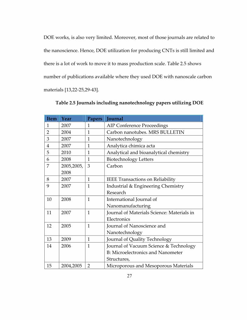
DOE works, is also very limited. Moreover, most of those journals are related to
the nanoscience. Hence, DOE utilization for producing CNTs is still limited and
there is a lot of work to move it to mass production scale. Table 2.5 shows
number of publications available where they used DOE with nanoscale carbon
materials [13,22-25,29-43].
Table 2.5 Journals including nanotechnology papers utilizing DOE
Item Year Papers Journal
1 2007 1 AIP Conference Proceedings
2 2004 1 Carbon nanotubes. MRS BULLETIN
3 2007 1 Nanotechnology
4 2007 1 Analytica chimica acta
5 2010 1 Analytical and bioanalytical chemistry
6 2008 1 Biotechnology Letters
7 2005,2005,
2008
3 Carbon
8 2007 1 IEEE Transactions on Reliability
9 2007 1 Industrial & Engineering Chemistry
Research
10 2008 1 International Journal of
Nanomanufacturing
11 2007 1 Journal of Materials Science: Materials in
Electronics
12 2005 1 Journal of Nanoscience and
Nanotechnology
13 2009 1 Journal of Quality Technology
14 2006 1 Journal of Vacuum Science & Technology
B: Microelectronics and Nanometer
Structures,
15 2004,2005 2 Microporous and Mesoporous Materials

28
16 2009 1 Polymer Letters
17 2007 1 Powder Technology
18 2007 1 Quality Progress
19 2006 1 Thin Solid Films
Most of the papers use full factorial design because of its understanding ease
and depth of information. Such technique is very useful for a technology in it
start like CNTs. Those designs are useful in most nanotechnology experiments
especially for the physical characteristics enhancements of innovative
nanostructures.
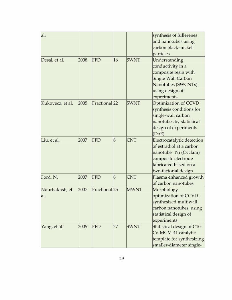
Table 2.6 illustrates instances of research using DOE and CNT. Table also 2.6
shows how most researchers often use the full factorial than other techniques.
Using fractional factorial design is used if the number of runs is high like for
two level seven factors experiment (27=128). However, this technique will help
when the full design with high number of runs is not feasible and the goal is to
get the main effects and low order factors interactions. Table 2.7 explains in
more details why some researchers use full or the other techniques.
Table 2.6 Publications using variable conventional processes and designs for
the optimization of carbon nanotubes characteristic [23-26,31,32,34,38,45-49]
Authors Year Design Runs TYPE Title
Cotasanchez, et 2005 FFD 16 BUCKY Induction plasma
29
al. synthesis of fullerenes
and nanotubes using
carbon black–nickel
particles
Desai, et al. 2008 FFD 16 SWNT Understanding
conductivity in a
composite resin with
Single Wall Carbon
Nanotubes (SWCNTs)
using design of
experiments
Kukovecz, et al. 2005 Fractional 22 SWNT Optimization of CCVD
synthesis conditions for
single-wall carbon
nanotubes by statistical
design of experiments
(DoE)
Liu, et al. 2007 FFD 8 CNT Electrocatalytic detection
of estradiol at a carbon
nanotube |Ni (Cyclam)
composite electrode
fabricated based on a
two-factorial design.
Ford, N. 2007 FFD 8 CNT Plasma enhanced growth
of carbon nanotubes
Nourbakhsh, et
al.
2007 Fractional 25 MWNT Morphology
optimization of CCVD-
synthesized multiwall
carbon nanotubes, using
statistical design of
experiments
Yang, et al. 2005 FFD 27 SWNT Statistical design of C10-
Co-MCM-41 catalytic
template for synthesizing
smaller-diameter single-

30
wall carbon nanotubes
Darsono, et al. 2007 FFD 8 CNT Field emission properties
of carbon nanotube
pastes examined using
design of experiments,
Gou, et al. 2004 FFD 8 BUCKY Experimental design and
optimization of
dispersion process for
single-walled carbon
nanotube bucky
dissertation
Cota-Sanchez, G 2003 FFD 16 MWNT Synthesis of carbon
nanostructures using a
high frequency induction
plasma reactor
Doddasanagouda
, S.
2006 FFD 8 SSNT Growth and
Deterministic Assembly
of Single Stranded
Carbon Nanotube
Kuo, et al 2005 Fractional 16 MWNT Diameter control of
multiwalled carbon
nanotubes using
experimental Design
Yang, et al. 2004 Fractional 28 SWNT Statistical analysis of
synthesis of Co-MCM-41
catalysts for production
of aligned single walled
carbon nanotubes
(SWNT)
Yeh, C. 2004 Fractional 30 Buckypaper CHARACTERIZATION
OF NANOTUBE
BUCKYDISSERTATION
MANUFACTURING
PROCESS

31
Table 2.7 Nano-manufacturing improvements techniques
Technique Nano-manufacturing
Fabrication method
Examples
Full Factorial Designs Those designs are useful in
most nanotechnology
experiments especially for the
physical characteristics
enhancements of innovative
nanostructures
Induction
Plasma (new
method but
currently with
low yield)
Fractional Factorial
Designs
This technique will help
when the full design high
number of runs is not
feasable and the goal is to get
the main effects and low
order factors interactions
Catalyst
Chemical vapor
deposition (big
number of
variables)
Non-Conventional
Designs
Such designs are used when
techniques efficiency is not
essential for the model
Injection
Molding (old
techniques)
An example of the use of full factorial can be seen in the dissertation about
Induction Plasma [33]. This process is new and currently has low yield in
comparison to other CNT synthesis methods. So, the author resolved to full
design to get the complete statistical analysis for factors interactions. In
contrast, other publications used fractional factorial for CVD. CVD is an old
technique with most variables is known and only small fraction of their
interactions is important [44].

32
Figure 2.12 Most researchers utilize Full Factorial designs for their
publications instead of other techniques like Fractional Factorial and Taguchi
In addition, there are some instances where some investigators used orthogonal
array to study CNT (See figure 2.11). Such designs are used when technique’s
efficiency is not essential for the model. For example, the Injection Molding
paper used an old technique’s where there is no need for a full statistical
analysis. Here the author can just study the new factors affecting the process
rather than studying all the factors. In addition, only suspected interactions are
examined since others might already have been proven insignificant. Figure
2.12 show an overview of the number of papers over the years who used
orthogonal arrays and Table 2.8 details their titles and other information.
RSM
Others
Fractional
FFD
Taguchi

33
Figure 2.13 Histogram of years 2004-2009 of papers related to Orthogonal
Arrays
Table 2.8 Summary of articles in the use of Orthogonal Arrays to optimize the
processes and designs related to carbon nanotubes [30,39,41,44,51]
Authors Year Array TYPE Title
Ting, et al. 2006 9 CNT Optimization of field
emission properties of
carbon nanotubes by
Taguchi method
Maheshwar, et al. 2005 18 CNT Application of the Taguchi
Analytical Method for
Optimization of Effective
Parameters of the Chemical
Vapor Deposition Process
Controlling the Production

34
of Nanotubes/Nanobeads
Lin, et al. 2006 9 Nano
fibers
Improvement on
superhydrophobic behavior
of carbon nanofibers via the
design of experiment and
analysis of variance
Jahanshahi, M 2007 16 CNT Application of Taguchi
Method in the Optimization
of ARC-Carbon Nanotube
Fabrication
Prashantha, K. 2009 16 MW
NT
Taguchi analysis of
shrinkage and warpage of
injection-moulded
polypropylene/multiwall
carbon nanotubes
nanocomposites
2.3.1 Experiments and Discussion
Three papers used DOE to optimize CNTs fabrication will be discussed here
[34, 36, 40]. The papers used two types of CVD to grow the CNTs, namely,
catalyst chemical vapor deposition (CCVD) and vertical chemical vapor
deposition (VCVD). Two papers research the use of CCVD to optimize the
diameter and synthesis condition of CNTs. Those papers have similar input and

35
output variables but one of them synthesized SWNT and the other MWNT.
Figure 2.13 shows a schematic of their CVD system.
Figure 2.14 Schematic diagram of the CCVD setup for carbon nanotube
synthesis
The third paper used VCVD, which has great promise for producing large
quantities of CNT. Its vertical setup allow for the constant feeding of the
catalyst material and carbon source to the furnace. However, it needs high
temperature to operate and its initial capital investment is high. Figure 2.14
shows how the vertical alignment is structured.

36
Figure 2.15 Schematic diagram of VCVD [50]
Both methods focused on the furnace temperature as an important factor to
study initially. Then, all of the research regardless of the analytical method used
concluded that it is a statistical significant factor. After that, the gas flow rate
was considered significant. For the CCVD a C2H2 source was utilized while the
VCVD used a methane source. Both the temperature and carbon source flow
rate ranges were moderately similar for the two processes. The third common
factor between the processes was carrier gas flow rate. Three gases were
considered. H2, N2 and Argon were varied dramatically between (50-2000Sccm)
to study their effect on CNTs. Table 2.9 summarizing the techniques used and
the results.

37
Table 2.9 CCVD and VCVD process for growing CNTs synthesis conditions,
MRL: mean rectilinear length, C%: Carbon Deposit, QDN: quality descriptor
number
Nourbakhsh et al. Kukovecz et al. Kuo et al.
Year 2007 2005 2005
Process CCVD CCVD VCVD
CNTs MWNT SWNT MWNT
Temperature
Co
700,800 850,900,950 1050,1150
Carbon
Source Flow
Rate
(3,12) C2H2 (5,10,15) C2H2 (125,250) CH4
Carrier Gas
Flow Rate
(50,110) C2H2 (100,300,500) Ar (1000,2000) N2
Runs 64 = 2
6-3
+BBD 128 = 27-4
+BBD 32 = 25-1
+CCD
Goal Diameter, MRL C%, QDN Diameter
(Kukovecz et al., 2005) used two level design with fractional factorial design
[23]. They optimize the main seven factors influencing the carbon percentage
and the ratio of radial breathing mode to the Raman spectrum d-band. The
seven factors are reaction temperature, reaction time, preheating time, catalyst
mass, C2H2 volumetric flow rate, Ar volumetric flow rate, and Fe: MgO molar
ratio. The design confounds three factors using BBD and so reduces the run to
22 instead of 128. Which is an example of DOE saving time and cost.
38
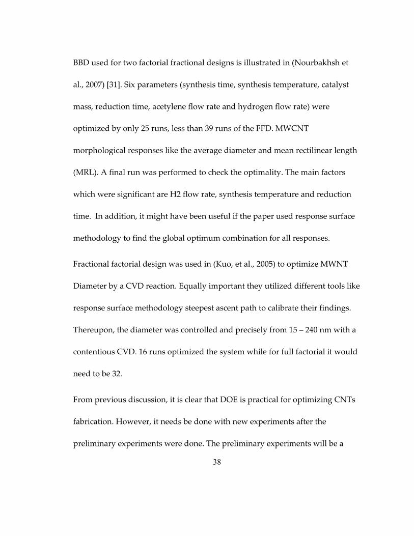
BBD used for two factorial fractional designs is illustrated in (Nourbakhsh et
al., 2007) [31]. Six parameters (synthesis time, synthesis temperature, catalyst
mass, reduction time, acetylene flow rate and hydrogen flow rate) were
optimized by only 25 runs, less than 39 runs of the FFD. MWCNT
morphological responses like the average diameter and mean rectilinear length
(MRL). A final run was performed to check the optimality. The main factors
which were significant are H2 flow rate, synthesis temperature and reduction
time. In addition, it might have been useful if the paper used response surface
methodology to find the global optimum combination for all responses.
Fractional factorial design was used in (Kuo, et al., 2005) to optimize MWNT
Diameter by a CVD reaction. Equally important they utilized different tools like
response surface methodology steepest ascent path to calibrate their findings.
Thereupon, the diameter was controlled and precisely from 15 – 240 nm with a
contentious CVD. 16 runs optimized the system while for full factorial it would
need to be 32.
From previous discussion, it is clear that DOE is practical for optimizing CNTs
fabrication. However, it needs be done with new experiments after the
preliminary experiments were done. The preliminary experiments will be a

39
used to setup the input and output factors of the DOE and their levels. With
ANN, we can utilize the preliminary results to build a process metamodel.
Then, we utilize metamodel to setup the DOE method and analysis. That
analysis will give us a better understanding of the CNTs fabrication without
having to do additional experiments. So, in the following chapters will be more
discussion on that metamodel and analysis.

40
3. Experimental Setup
This chapter will discuss growing VA-SWNTs experimental Setup and CVD
setup. First, we describe the details of the growth system variables. Then, we
discuss the catalyst preparation and generalization of the CVD setup especially
the growth processes. The length controlled VA-SWNTs were synthesized by
using an ethanol CVD technique.
Most of the experiment setup here is similar to work published before utilizing
ethanol based CVD to grow VA-SWNTs [23, 46]. Figure 3.1 is a schematic
showing the ethanol CVD system and experimental procedure for the growth
of the highly aligned CNTs.
41
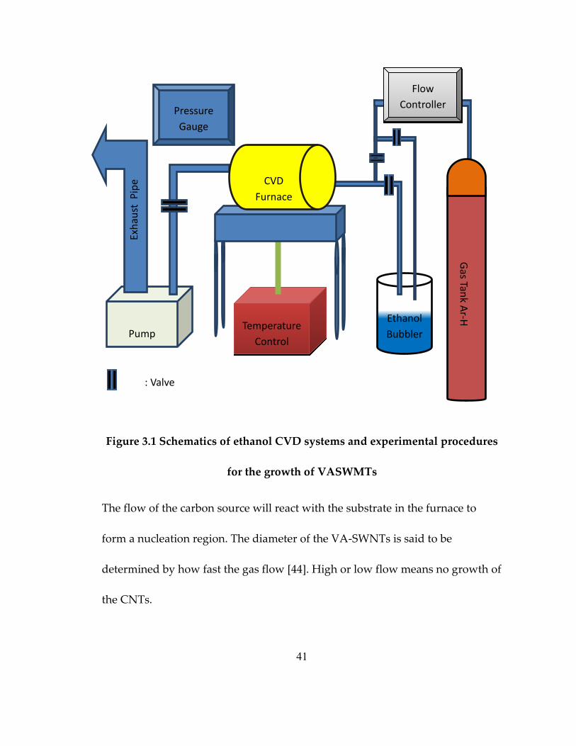
Figure 3.1 Schematics of ethanol CVD systems and experimental procedures
for the growth of VASWMTs
The flow of the carbon source will react with the substrate in the furnace to
form a nucleation region. The diameter of the VA-SWNTs is said to be
determined by how fast the gas flow [44]. High or low flow means no growth of
the CNTs.
Pump
Ethanol
Bubbler
Gas Tan
k Ar-H
Flow
Controller Pressure
Gauge
Temperature
Control
: Valve
Exh
aust
Pip
e
CVD
Furnace

42
3.1 System Variables
Figure 1.1 shows the input-output diagram of the CVD process to grow VA-
SWNTs. As shown in the figure, temperature, gas flow rate and pressure are
considered the important process inputs. VA-SWNTs length is considered the
key performance indicator, i.e. process output.
Input Variables
1. CVD temperature: It is the temperature of the gas flowing through the furnace;
it is measured by a thermocouple installed inside the furnace; the resolution of
this measurement is 1°C.
2. Gas flow rate: it is the volumetric flow rate of the gas flowing through the
furnace; it is measured by flow gauge; the unit of this measurement is Standard
Cubic Centimeters per Minute (SCCM).
3. CVD pressure: it is the furnace pressure at the time of CNT growth; it is
measured by a pressure gauge attached to the furnace; the control resolution of
this apparatus is 1 Torr.
4. Growth time: It is the duration from the time the substrate is inserted in to the
furnace until the process is terminated; it is measured in minutes.

43
Noise Factors
Noise factors are known or unknown variables affecting the VA-SWNTs
growth and they have one thing in common; they are uncontrollable. Lot of
variables affect the sample before, during, and after growth. Some are inside the
furnace like the ambient temperature and rate of cooling. Others are from the
environment like the gravity field. A Cause and Effect Diagram (Fishbone)
Analysis is done to map each input variable to the output. The major inputs are
classified to Measurement, Method, Machine, Manpower, Materials, and
Environment. As shown in Figure 3.2 an analysis investigation is done on each
of those inputs to study and classify the most important of them. More
emphasis is aimed to classify them to either controllable or non-controllable
(noise) factors.

44
Figure 3.2 Cause and effect matrix of input variables

45
3.2 Catalyst Preparation
Catalyst system is prepared by sputter coating a 20 nm thick Aluminum layer
onto a SiO2 wafer as a buffer to grow VA-SWNTs. Then, the layer is exposed to
the air for the formation of aluminum oxide. Using a sputter coater a 0.5-1 nm
thick Cobalt (Co) catalyst film was deposited on top of the Al/SiO2 layer with
wide dispersion. Figure 3.3 shows a schematic of the preparation process.
Figure 3.3 Schematic of the cross section of the substrate
3.3 CVD Process Setup
CVD setup is done through the following steps. First, put the substrate inside
the furnace. Then, pressurize the furnace to prepare for the growth process.
Meanwhile, a mixture of an argon-hydrogen (5% hydrogen) is supplied as the
carrier gas to maintain the pressure at 700 Torr. Consequently, the temperature
SiO2
AL
Co

46
inside the quartz tube furnace reaches 850°C. After that, a controlled high-
purity anhydrous ethanol (99.95%) vapor is supplied from the bubbler as a
carbon source for the growth of VA-SWNTs. Using different
ethanol/argon/hydrogen mixture gas flow rates, different VA-SWNTs are
synthesized. Resulting VA-SWNTs shown in two views and set of samples is
shown in Appendix A. Also, Appendix A shows a set of pictures showing the
whole CVD system, heat source and temperature sensor, pressure machine,
gases locker, the ethanol bubbler, the gold plated furnace, the catalyst sputter.

47
4. Process Design for Controllability
In this dissertation, we study the controllability of VA-SWNTs growth via a
hybrid process model of an experimental design and an artificial neural
network (ANN). Controllability here means to selectively fabricate only VA-
SWNTs. Our process analysis shows that CVD pressure and temperature are
the most significant input factors [47]. In addition, interactions and response
surface plots confirm these results and show that higher temperature and
pressure will yield VA-SWNTs with high probability.
Our proposed approach aims to analyze experimental data from a CVD
process, build neural network models, and perform statistical analysis with the
goal of relating the CVD input parameters to the characteristics of the CNTs to
gain better understanding of CNT properties. Our objective is to evaluate all
input variables theoretically and experimentally to find the statistically
significant ones.
The proposed methodology has two distinct stages. Stage 1 focuses on building
a metamodel of the process using the experimental data and an ANN technique
such as an MLP. A metamodel in this context captures the overarching behavior
of the process by broadly encompassing the data available at hand. Using the

48
metamodel, Stage 2 generates multiple runs for a full-factorial experimental
design.
4.1 Metamodel and Design of Experiments
Artificial Neural Network Design Stage
The following are the steps that make up the stage 1 of the research
methodology.
Delete records with missing data.
Using the records retained in the previous step, train a set of MLPs for
predicting the process outputs; given that input vectors are positioned
densely in the input space, the neural networks is likely to learn the
mapping between process inputs and outputs accurately.
Compute the prediction accuracy of each MLP and retain the network that
gives the highest prediction accuracy.

49
The neural network selected in the previous step serves as a meta-model of
the process. Compute the paired difference between the actual process
outputs and the neural-network estimated process responses.
Conduct the t-test on paired differences with level of significance = 0.05.
H0: d = 0 and H1: d > 0, where d is the mean of the paired differences.
Compute t0, the t-statistic for the paired difference. If |t0|> tα/2 then reject
H0; otherwise we fail to reject H0, and conclude that our metamodel is a
viable statistical representation of the experiment.
Design of Experiment Stage
After building the MLP-based process metamodel, a DOE study is performed.
Following are the steps required for their implementation.
Find the min-, mid- and max-points of each input variable for the records
used for training the selected neural networks in stage 1.
Create the level settings for the DOE using the min-, mid-, and max-points
of the input variables.
Conduct DOE analysis using the DOE runs.

50
System Variables
The process input variables are growth time; furnace temperature, gas flow
rate, and chamber pressure (see Figure 1.1). The process output is one of three
possible types on of CNTs : VA-SWNTs, MWNTs or MWNTs-SWNTs mixture.
Seven hundred and fifty samples of VA-SWNTs were used in our study (see
Appendix B). First, we eliminated the records that lack measurement quality or
completeness of data. This brought down the number of available records to
702. We ignored the growth time since it has no effect on the type of CNTs that
come out of the process. Using these records, we trained an MLP neural
network with three input nodes, four output nodes, and a different number of
hidden neurons. We found that an MLP with three inputs, seven hidden nodes,
and four outputs (3-7-4) gives the best prediction (83%) for the training data as
shown in Figure 4.1.

51
Figure 4.1 Classifications accuracy of process outcome
The ANN response is obtained from the trained MLP. Then, we computed the
response estimation error (the absolute difference between the predicted and
actual values) for the prediction. Subsequently, the paired t-test was conducted
on the actual process output and the neural-network estimated process
responses. We computed t0 for the VA-SWNTs and found it to be t0= 0.76. So,
the value of |t0| < t0.025= 1.98, and hence we concluded that there is no statistical
evidence to say that the behavior of the metamodel is different from that of the
actual process. This has given us the confidence that the DOE analysis
conducted using metamodel will be statistically valid.
0%
20%
40%
60%
80%
100%
MWNTs &SWNTs
MWNTs VA-SWNTs None PredictionAccuracy
Cla
ssif
icat
ion
Acc
ura
cy
52
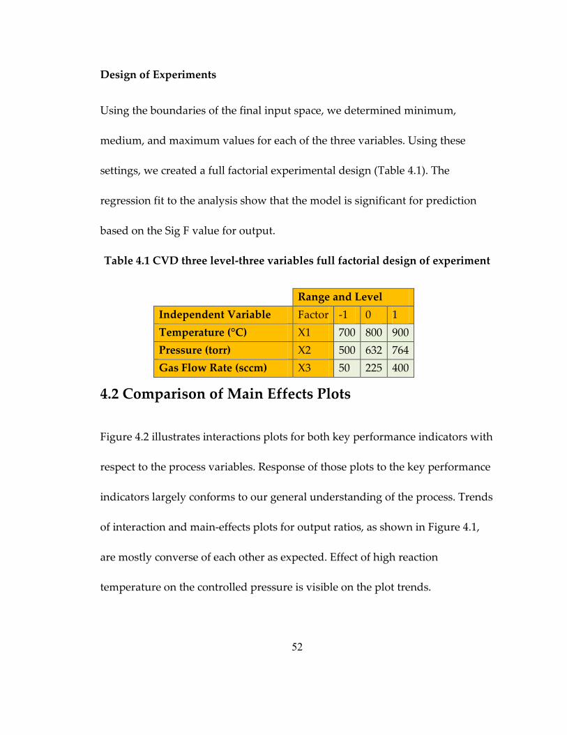
Design of Experiments
Using the boundaries of the final input space, we determined minimum,
medium, and maximum values for each of the three variables. Using these
settings, we created a full factorial experimental design (Table 4.1). The
regression fit to the analysis show that the model is significant for prediction
based on the Sig F value for output.
Table 4.1 CVD three level-three variables full factorial design of experiment
Range and Level
Independent Variable Factor -1 0 1
Temperature (°C) X1 700 800 900
Pressure (torr) X2 500 632 764
Gas Flow Rate (sccm) X3 50 225 400
4.2 Comparison of Main Effects Plots
Figure 4.2 illustrates interactions plots for both key performance indicators with
respect to the process variables. Response of those plots to the key performance
indicators largely conforms to our general understanding of the process. Trends
of interaction and main-effects plots for output ratios, as shown in Figure 4.1,
are mostly converse of each other as expected. Effect of high reaction
temperature on the controlled pressure is visible on the plot trends.

53
700. 800. 900.
Temperature (°C)
VA-SWNT
MWNTs
SWNTs & MWNTs
none
Pressure (torr) 500.
Pressure (torr) 632.
Pressure (torr) 764.
Figure 4.2 Interaction Plots between Temperature and Pressure for VA-
SWNTS
Interaction plot serves as a secondary means to gauge the efficacy with which
our metamodel simulate the actual process behavior in response to the changes
in the input settings. Once we have the interaction plots for the generally
anticipated behavior of the process, we go into variable specific analysis within
the input variables space defined by the minimum and maximum values
available in the experimental data.

54
4.3 Pareto and General Response Surface Plots
The R-squared value for the process is 0.89 and the standard error is 0.15. The
Pareto chart of the analysis is presented in Figure 4.3. The Figure shows that
CVD temperature and pressure are the most statistically significant factors ( =
0.05). Therefore, any alteration of their values will affect the desired output
(VA-SWNTs). Response surface plots in Figure 4.4 help illustrate the details of
the growth changing aspects of VA-SWNTs with respect to individual behavior
of the control variables. The figure shows that there is a more rapidly increasing
ascent of the VA-SWNTs response surface along increasing temperature and
pressure. This provides insight into the role of high temperature and pressure
and its positive impact on VA-SWNTs growth.

55
0.00 0.02 0.04 0.06 0.08 0.1
Absolute Coefficient
F
T by F
P2
T2
T by P
T
Desig
n E
ffects
T= Temperature (°C)
P= Pressure (torr)
F= Flow Rate (sccm)
Figure 4.3 Process Analysis Pareto Plot
Figure 4.4 Response Surface Plots of VA-SWNTs Length (Temperature VS
Pressure)

56
5. Process Design for Length Assurance
Chapter 4 researched the VA-SWNTs controllability while this chapter will
research their length assurance. Chemical vapor deposition (CVD) is one of the
several viable methods for growing VA-SWNTs. Utilizing Co supported on
multilayer Al/SiO2 as the catalyst and a hydrocarbon feedstock, VA-SWNTs are
grown in excess of a millimeter high. To control VA-SWNTs length, one has to
use the right combination of process inputs such as hydrocarbon flow, growth
time, temperature, and pressure.
This dissertation presents a process metamodel-based full factorial
experimental design and analysis to study the yield of tall VA-SWNTs. All of
the process variables under the study play a role in influencing VA-SWNTs
length; the current study which under review in the “International Journal of
Advanced Manufacturing Technology” investigates their main effects and
interactions [48]. The neural network metamodel-based analysis demonstrates
that the hydrocarbon flow rate and the pressure are the most statistically
significant factors that influence the length of VA-SWNTs. In addition, the
response surface graph confirms the factors of significance and adds that higher
flow with lower pressure will consistently yield tall VA-SWNTs.

57
We found that gas flow rate is the most significant of the control variables and
only the optimum value of the gas flow can ensure the growth of tall VA-
SWNTs. We also found that the interaction of flow rate with temperature of the
gases in the chamber is extremely significant to the quality of output indicating
towards velocity related dynamic pressure of the fluid to be a way to simplify
the understanding of the process. Outcomes of this investigation are beneficial
for moving closer to producing VA-SWNTs on production scale.
5.1 Metamodel and Design of Experiments
The methodology employed [26] has two phases. Phase 1 focuses on building
the process metamodel using the experimental data. The metamodel in this
context captures the overarching behavior of the process by broadly
encompassing the data available at hand. Using the metamodel, in Phase 2 we
generate multiple runs for a full-factorial experimental design to study the
influence of the process input variables (Figure 5) on the length of the VA-
SWNTs.
We explored different data modeling techniques keeping in view that the
anticipated behavior of the control variables is highly nonlinear. First technique
we considered is non-parametric regression, which is one of the most

58
established modeling techniques in statistical theory as presented by Dasguta et
al. [27]. However, its dependence on the valid statistical design of training data
is the major challenge to its applicability to the problem at hand. The basic
fitting parameter, i.e. R2 for the response surface regression with linear, paired
interaction and nonlinear coefficients was 0.32, a low number of valid results.
Thus, we use neural networks as an alternative modeling technique.
There are different types of neural networks like self-organizing maps and
radial basis functions that can be used for modeling process input-output
relationship [28]. Most MLPs contain highly connected feed-forward
connections with a layer of input nodes, one or more layers of hidden nodes,
and a layer of output nodes [29]. The input signal propagates forward layer-by-
layer with every node in the hidden and output layers representing a smooth
and differentiable nonlinear activation function.
Therefore, we used multi-layer perceptron based on back propagation
algorithm, which is well known as a universal approximate of the non-linarites
in the training data. Using these experimental data records, we trained multi-
layer perceptions with three input nodes, one output node. The architecture of
the MLP used in the current dissertation is shown in Figure 5.1.

59
Figure 5.1 Architecture of a multi-layer perceptron network
As shown in Figure 5.2 R2 value of 0.5 for the network architecture with three
input nodes, 21 hidden nodes and one output node renders it as a better meta-
model for the process with the available data at hand. Once the best available
process meta-model is selected, we used a full factorial design of experiments to
design a set of computer experiments with 30 replication for each record for
studying the details of process behavior. We compute t0 for the VA-SWNTs
length and find It to be t0 = 0.9188. So, the value of |t0| < t0.025= 1.98. On this
basis, we decide that there is no statistical evidence to say that the behavior of
the metamodel is different from that of the actual process with 97.25%
confidence level.

60
Scatterplot of VA-SWNTs Length againest Estimated VA-SWNTs Length
y = -51.4918+1.015 * x; R = 0.7026; R2 = 0.4936; 0.95 Prediction Interval
0 200 400 600 800 1000 1200
Estimated VA-SWNTs Length
0
200
400
600
800
1000
1200V
A-S
WN
Ts
Len
gth
Figure 5.2 VA-SWNTs length (target) versus estimated VA-SWNTs length
(output) regressions graph for the MLP 4-21-1 network
Metamodel
The following are the steps to construct the computer model:
Eliminate experimental data records with missing data.
Normalize the values of each process control variable in [0, 1] range. This
transformation brings all control variables into the same numerical range to
give equal weight to each variable in clustering process described below.
61
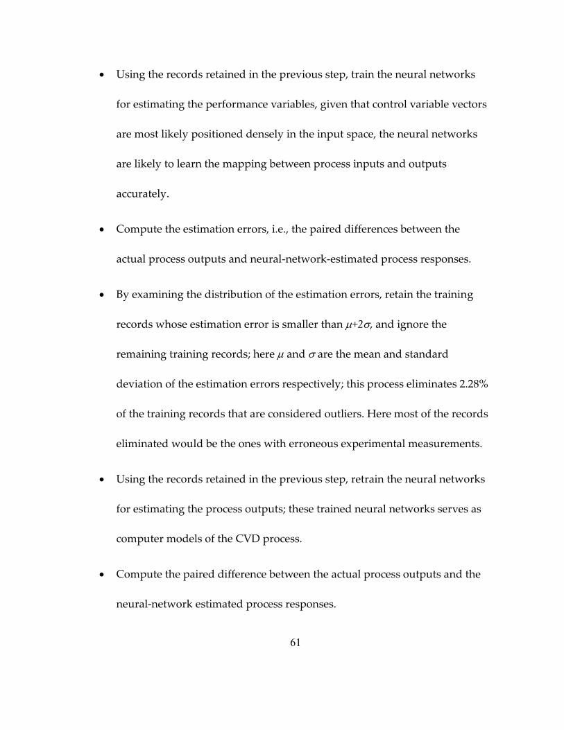
Using the records retained in the previous step, train the neural networks
for estimating the performance variables, given that control variable vectors
are most likely positioned densely in the input space, the neural networks
are likely to learn the mapping between process inputs and outputs
accurately.
Compute the estimation errors, i.e., the paired differences between the
actual process outputs and neural-network-estimated process responses.
By examining the distribution of the estimation errors, retain the training
records whose estimation error is smaller than +2, and ignore the
remaining training records; here and are the mean and standard
deviation of the estimation errors respectively; this process eliminates 2.28%
of the training records that are considered outliers. Here most of the records
eliminated would be the ones with erroneous experimental measurements.
Using the records retained in the previous step, retrain the neural networks
for estimating the process outputs; these trained neural networks serves as
computer models of the CVD process.
Compute the paired difference between the actual process outputs and the
neural-network estimated process responses.

62
Conduct the t-test on paired differences with a level of significance, say =
0.05 (this can be tightened or relaxed if necessary). H0: d = 0 and H1: d > 0,
where d is the mean of the paired differences. Compute t0, the t-statistic for
the paired difference. If |t0|> tα/2 then reject H0; otherwise we fail to reject H0,
which would mean that statistically we do not have evidence to the effect
that the behavior of the metamodel is different from that of the actual
process.
Design of Experiment Phase
After building the multi-layer perceptron based process metamodel, we
perform a design of experiment study. The following steps are used to conduct
the study.
Find the min-, mid- and max-points of each input variable for the records
used in training the neural networks in phase 1.
Create the three level settings for the DOE using the min-, med-, and max-
points of the input variables.
Create 30 replications of each pattern by adding a Gaussian noise to each
variable. The Gaussian noise was added with mean equal to zero and

63
standard deviation equal to 1% of the minimum value of each variable in the
training data.
Conduct DOE analysis using the DOE runs.
We started with 100 records of VA-SWNTs growth using the same
experimental setup for chapter 3 (See Appendix C). First, we eliminated records
with errors in measurements and missing data. This brought down the number
of available records to 84 samples. The distribution of the control variables in
these 84 records is shown in Figure 5.3.
873 876 879 882 885 888 891 894 897
CVD Temperature (°C)
0
10
20
30
40
50
60
70
80
90
No
of
Ob
se
rv
at
ion
s
700.0 706.4 712.8 719.2 725.6 732.0 738.4 744.8 751.2 757.6 764.0
CVD Pressure (Torr)
0
10
20
30
40
50
60
70
No o
f O
bserv
ations

64
50 85 120 155 190 225 260 295 330 365 400
Gas Flow Rate (torr)
0
10
20
30
40
50
60
70
80
No of
Obs
erva
tions
Figure 5.3 Histograms showing the distribution of control variables in the
training data for neural networks
Using the boundaries of the final input space, we determine minimum,
medium, and maximum values for each of the four input variables. Table 5.1
shows the min, mid, and max values of the records used for the analysis.
Table 5.1 Experimental records of the CVD process input and output
variables
Variable Min Mid Max
CVD Temperature (°C) 870 889 900
CVD Pressure (sccm) 700 717 764

65
Gas Flow Rate (Torr) 50 97 400
5.2 Pareto Chart Analysis
The comparison of significance of control variables, their quadratic effects, and
or their paired interactions is presented in Pareto and the coefficients of
regression Figure 5.4. The most significant of the variables is the quadratic
effect of the gas flow in the chamber during growth. After that linear effect of
chamber pressure, interaction of pressure and flow and linear effect of chamber
pressure bear almost the same significance of effect on the length of VA-SWNTs
grown.
Figure 5.4 Process Pareto Analysis, (A) CVD Temperature (°C), (B) CVD
Pressure (sccm), (C) Gas Flow Rate (Torr)
66
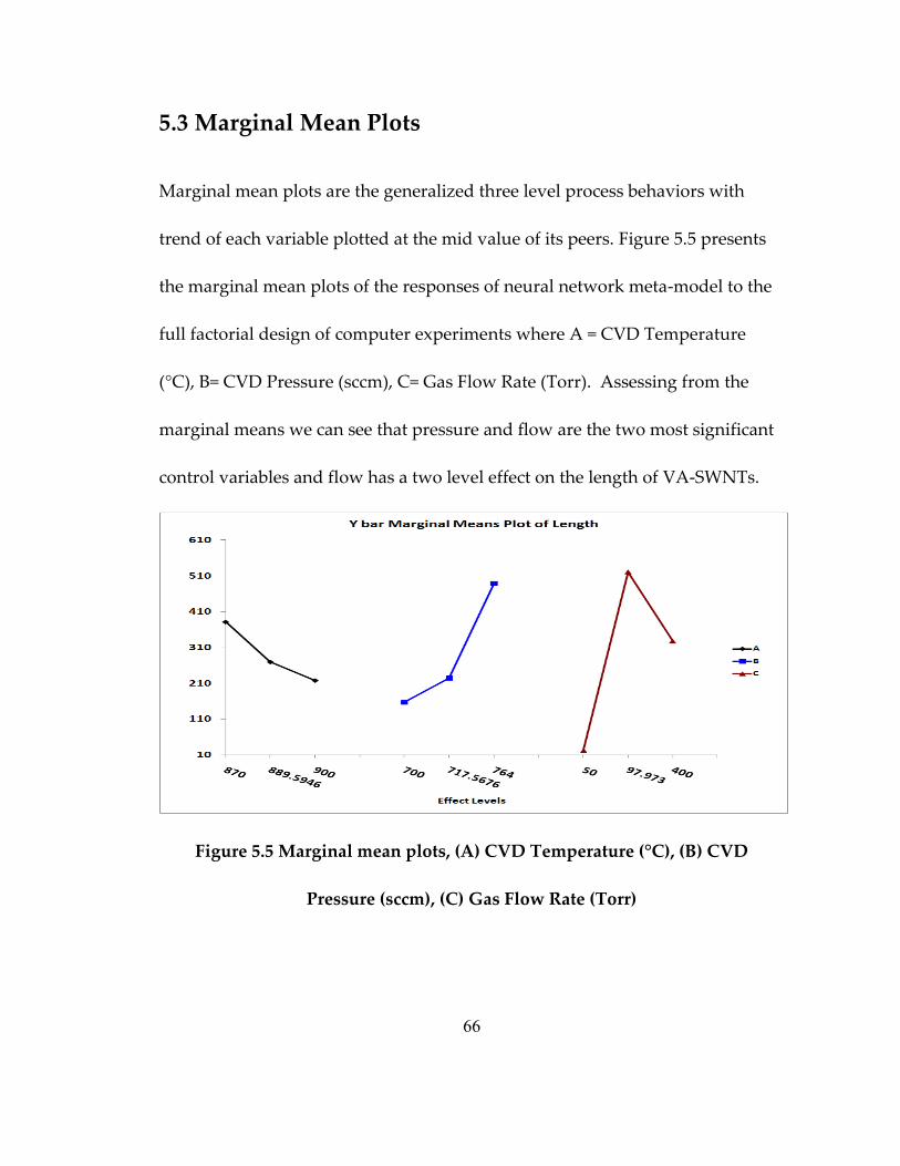
5.3 Marginal Mean Plots
Marginal mean plots are the generalized three level process behaviors with
trend of each variable plotted at the mid value of its peers. Figure 5.5 presents
the marginal mean plots of the responses of neural network meta-model to the
full factorial design of computer experiments where A = CVD Temperature
(°C), B= CVD Pressure (sccm), C= Gas Flow Rate (Torr). Assessing from the
marginal means we can see that pressure and flow are the two most significant
control variables and flow has a two level effect on the length of VA-SWNTs.
Figure 5.5 Marginal mean plots, (A) CVD Temperature (°C), (B) CVD
Pressure (sccm), (C) Gas Flow Rate (Torr)

67
5.4 Comparison of Main Effects Plots
In order to investigate the details of interaction between chamber pressure and
flow of the constituent gases (Ethanol, Hydrogen, and Argon), we performed
the main effects analysis on this interaction. Figure 5.6 shows the interaction
plots for the key performance indicator (length of VA-SWNTs) with respect to
the significance process variables, namely, pressure and flow rate. The
interaction plots largely confirm our belief that the process pressure and flow
rate are the most influential process input parameters. The sensitivity trends of
chamber pressure, which directly relates to the availability of gases for growth
reaction at min, mid, and max values of net flow rate of the gases, indicate
towards the details of nature of two level effect of the flow rate on the length of
the VA-SWNTs. The minimum extreme of flow rat e, which in a way indicates
towards the sustained supply of fresh mix of gases, shows almost no growth.
However, the extreme high-end values of the flow, i.e., 400 sccm refer to a
saturation effect that can be forced to yield taller SWNTs if coupled with higher
pressure. Pressure here seems to ensure sustained concentration of reactant at
catalyst locations to maintain the growth mechanism. The fundamental
conclusion which we can draw form this is that the velocity of arriving

68
constituent atoms at the cobalt catalyst locations needs to be maintained high
but the momentum must not exceed the strength of the van der Walls forces
that initiate and maintain the growth reaction. However, this growth
phenomenon appears to optimize the length of VA-SWNTs grown at the
optimum range of flow rate (225 sccm) revealing that pressure may only ensure
the supply of right amount of constituent atoms to some extent. The main
influences that flow rate has on the growth phenomenon are ensuring the
optimum compensation of reaction constituents to the depleted stoichiometry
in the vicinity of the catalyst location and guaranteeing the right amount of
momentum these atoms have.
Figure 5.6 Main effect plots for VA-SWNTs length of pressure and flow
-10
490
990
1490
700 704 707 711 714 718 721 725 728 732 736 739 743 746 750 753 757 760 764
Re
spo
nse
Val
ue
B
Length Y-hat Interaction Plot B vs C
Constants: A = 885
50
225
400

69
5.5 General Response Surface Plot
A. Response Surface (Length versus Flow and Pressure)
A further deeper and concise insight in the growth mechanism can be attained
by analyzing the response surface between chamber pressure and flow rate and
the length of the VA-SWNTs as shown in the Figure 5.7. The minimum and
maximum values of the chamber pressure are not significant in terms of the
concentrating effect they may have on the flowing mixture of gases with very
small flow rate, i.e., 50 sccm. Similarly, at the highest flow rate values in the
training data, i.e., 400 sccm stepping the chamber pressure up to 764 Torr can
support the growth reaction to the extent that the resultant VA-SWNTs length
of 900 µm can be achieved as explained in Figure 10. However, the two level
effect of the flow rate can optimize the length to 990 µm and ≈ 1390 µm at 700
Torr and 764 Torr respectively.

70
Figure 5.7 Response surface plot of VA-SWNTs length VS flow rate VS
pressure
B. Response Surface (Length w.r.t Flow and Temperature)
In order to further test the theory of effect of momentum on the van der Waals
forces that ensure the stiction of incoming constituent atoms at the cobalt
location, we investigated the impact of temperature on the flow of the gases in
the chamber even though the temperature turned out to be the relatively
insignificant variable in the Pareto of coefficients (Figure 5.4). Figure 5.7 is the
response surface of the length w.r.t flow and temperature at the mid setting of
the pressure of constituent gases in the chamber, i.e., 732 Torr. Figure 5.8 is the

71
main effect plot of the two control variables in order to elaborate the
significance of impact of temperature on flow of constituents along the hidden
edge of the response surface in Figure 5.9. As anticipated, the impact of
temperature on the dominant nonlinear flow rate is minimum at the optimum
flow rate, i.e., 225 sccm. However, its impact is magnified where the a large
amount of constituents is arriving at the cobalt locations with already too high
momentum and the temperature only adds to the volatility of the saturation
condition of the supply of constituents.
Figure 5.8 Main effect plots for VA-SWNTs length of temperature and flow
-10
190
390
590
790
990
1190
1390
870872873875877878880882883885887888890892893895897898900
Re
spo
nse
Val
ue
A
Length Y-hat Interaction Plot A vs C
Constants: B = 732
50
225
400

72
Figure 5.9 Response surface plot of VA-SWNTs length VS flow rate VS
temperature
50
147.2222222
244.4444444341.6666667
-10
490
990
1490
87
0
87
3
87
7
88
0
88
3
88
7
89
0
89
3
89
7
90
0
C
Re
spo
nse
Val
ue
A
Length Y-hat Surface Plot A vs C
Constants: B = 732
990-1490
490-990
-10-490

73
6. Process Design for CVD Flow
This chapter discusses in depth the relation between the gas flow and time. The
methodology employed [26] has two phases and somewhat similar to the one
employed in the previous chapter.
As shown in Figure 6.1 R2 value of 0.8 for the network architecture with two
input nodes, 12 hidden nodes and one output node renders it as a better meta-
model for the process with the available data on hand (See Appendix D). Once
the best available process meta-model is selected, we used a full factorial design
of experiments to design a set of computer experiments for each record for
studying the details of process behavior. We compute t0 for the VA-SWNTs
length and find it to be t0 = 0.17. So, the value of |t0| < t0.025= 1.98. On this basis,
we decide that there is no statistical evidence to say that the behavior of the
metamodel is different from that of the actual process with 97.25% confidence
level.

74
Scatterplot of VA-SWNTs Length againest Estimated VA-SWNTs Length
y = -97.9+0.08 * x; R = 0.89; R2 = 0.8; 0.95 Prediction Interval
300 350 400 450 500 550 600 650 700
Actual VA-SWNTs Length
300
350
400
450
500
550
600
650
700
Estim
ate
d V
A-S
WN
Ts L
ength
Figure 6.1 VA-SWNTs length (target) versus estimated VA-SWNTs length
(output) regressions graph for the MLP 2-12-1 network
The following are the steps to construct the computer model:
Eliminate experimental data records with missing data.
Normalize the values of each process control variable in [0, 1] range. This
transformation brings all control variables into the same numerical range to
give equal weight to each variable in clustering process described below.
Using the records retained in the previous step, train the neural networks
for estimating the performance variables; given that control variable vectors

75
are most likely positioned densely in the input space, the neural networks
are likely to learn the mapping between process inputs and outputs
accurately.
Compute the estimation errors, i.e., the paired differences between the
actual process outputs and neural-network-estimated process responses.
Using the records retained in the previous step, retrain the neural networks
for estimating the process outputs; these trained neural networks serves as
computer models of the MBE process.
Compute the paired difference between the actual process outputs and the
neural-network estimated process responses.
Conduct the t-test on paired differences with a level of significance, say =
0.05 (this can be tightened or relaxed if necessary). H0: d = 0 and H1: d > 0,
where d is the mean of the paired differences. Compute t0, the t-statistic for
the paired difference. If |t0|> tα/2 then reject H0; otherwise we fail to reject H0,
which would mean that statistically we do not have evidence to the effect
that the behavior of the meta model is different from that of the actual
process.

76
Design of Experiment Phase
After building the multi-layer perceptron based process metamodel, we
perform a design of experiment study. The following steps are used to conduct
the study.
Find the min-, mid- and max-points of each input variable for the records
used in training the neural networks in phase 1.
Create the three level settings for the DOE using the min-, med-, and max-
points of the input variables.
Conduct DOE analysis using the DOE runs.
We started with 42 records of VA-SWNTs growth using the experimental
setup described in chapter 3. First, we eliminated records with errors in
measurements and missing data. This brought down the number of
available records to 25 samples.
Using the boundaries of the final input space, we determine minimum,
medium, and maximum values for each of the four input variables. Table 1
shows the min, mid, and max values of the records used for the analysis.

77
Table 6.1 Experimental records of the CVD process input and output
variables
Variable Min Mid Max
Growth Time (min) 5 32 60
Gas Flow Rate
(Torr) 20 85 150
6.1 Pareto Chart Analysis
The comparison of significance of control variables, their quadratic effects, and
or their paired interactions is presented in Pareto and the coefficients of
regression Figure 6.2. The most significant of the variables is the quadratic
effect of the time and gas flow in the chamber during growth.
p=.05
Standardized Effect Estimate (Absolute Value)
t
F2
F by t
F
t2
t= T ime (min) F= Flow Rate (sccm)
Figure 6.2 Process Pareto analysis

78
6.2 Comparison of Main Effects Plots
In order to investigate the details of interaction between growth time and gas
flow we performed the main effects analysis on this interaction. Figure 6.3
shows the interaction plots for the length of VA-SWNTs with respect to the
process input variables, namely, time and flow rate. The sensitivity trends of
growth time, which directly relates to the availability of gases for growth
reaction at min, mid, and max values of net flow rate of the gases, indicate
towards the details of nature of time low level effect of the flow rate on the
length of the VA-SWNTs.
Time 5. Time 32.5 Time 60.
20. 85. 150.
Flow
0
100
200
300
400
500
600
700
800
900
1000
Le
ng
th
Figure 6.3 Main effect plots for VA-SWNTs length of time and flow

79
6.3 General Response Surface Plot
A further deeper and concise insight in the growth mechanism can be attained
by analyzing the response surface between growth time and flow rate and the
length of the VA-SWNTs as shown in the Figure 6.4. The minimum and
maximum values of the growth time are not significant in terms of the
concentrating effect they may have on the flowing mixture of gases with flow
rate. Higher VA-SWNTs length will be achieved at less than 20 minute and flow
rate fewer than 150 sccm. This would be suitable for repeatedly producing
medium length VA-SWNTs.
> 800 < 780 < 680 < 580 < 480 < 380 < 280 < 180
Figure 6.4 Response surface plot of VA-SWNTs length VS flow rate VS time

80
7. Scientific Formulation of the Process Input
Variables
Previous chapters discuss the CVD grown VA-SWNTs input and output
variables. In addition, they discuss which of them are most significant for the
controllability or the length assurance. We used the pressure gauge to check the
reliability of the pressure sensor during the growth time. We found that the
pressure sensor is slightly fluctuating. Therefore, an investigation of the
fluctuating was performed to Figure out if the setup value is a good
representative of the CVD pressure. The following Figure 7.1 shows that the
pressure average of two 30 minutes runs. From figure it is clear that the
fluctuation is between 680 torr and 730 torr for a setup value of 700 torr. This
mean that we can approximate the pressure by its setup value. Therefore, we
used the setup value as a measure of the CVD pressure. The exact values
observed for the two runs are shown in appendix E.

81
Figure 7.1 First and second runs graphs to measure the stability of pressure
sensor during VA-SWNTs growth time (average = 705.2 torr, 703.5 torr)
Based on the plots of marginal means, interactions, and response surfaces the
overall relationship between the VA-SWNTs controllability and length with the
four controlled inputs can be iterated as follows:
680
690
700
710
720
1 3 5 7 9 11 13 15 17 19 21 23 25 27 29
CV
D P
ress
ure
(to
rr)
Growth Time (min)
Pressure
Pressure
Linear (Pressure)
680
690
700
710
720
1 3 5 7 9 11 13 15 17 19 21 23 25 27 29
CV
D P
ress
ure
(to
rr)
Growth Time (min)
Pressure
Pressure
Linear (Pressure )
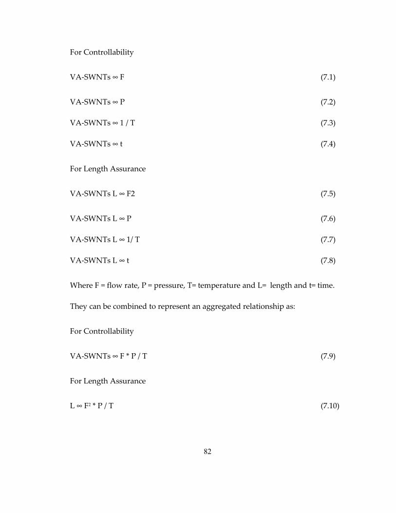
82
For Controllability
VA-SWNTs ∞ F (7.1)
VA-SWNTs ∞ P (7.2)
VA-SWNTs ∞ 1 / T (7.3)
VA-SWNTs ∞ t (7.4)
For Length Assurance
VA-SWNTs L ∞ F2 (7.5)
VA-SWNTs L ∞ P (7.6)
VA-SWNTs L ∞ 1/ T (7.7)
VA-SWNTs L ∞ t (7.8)
Where F = flow rate, P = pressure, T= temperature and L= length and t= time.
They can be combined to represent an aggregated relationship as:
For Controllability
VA-SWNTs ∞ F * P / T (7.9)
For Length Assurance
L ∞ F2 * P / T (7.10)
83
7.1 Ideal Gas Law
We can derive an approximate equation from the Ideal Gas Law formula [52].
That law is part of the thermodynamics theory relating pressure, temperature,
and volume.
P * Vol = n * Ru * T (7.11)
Where Ru = specific gas constant , Vol= volume of gases, and n = chemical
amount of gases. Since volume is the multiplication between flow and cross
sectional area of the system (A).
Vol = F * A (7.12)
Substituting all the values, we get the following formula:
P * F * A = n * Ru * T (7.13)
Assuming that n and Ru divided by A is proportional to the desired output, we
rewrite it as:
P * F / T = n * Ru / A (7.14)
Figure 7.1 shows the slight correlation between controllability of VA-SWNTs
and the above formulation extracted from the ideal gas law.

84
Matrix Plot
700 800 900 1000
101
102
103
104
500 588 676 764
101
102
103
104
25 183 342 500
101
102
103
104
25 37 48 60
101
102
103
104
Temperature (°C) Pressure (torr) Flow Rate (sccm) Time (min)
Result
Figure 7.2 Matrix plots between flow, temperature and pressure for VA-
SWNTS (101 = VA-SWNTs, 102 = MWNTs, 103 = MWNTs & SWNTs, 104 =
None)
This refers to a possibility of relationship between the macro scale physical
quantity of the gases in the CVD chamber and quantum level phenomenon.
Our detailed designed experimental studies corroborated this hypothesis,

85
which explains the physics of the growth process for customization chamber
designs for high rate manufacturing.
7.2 Dynamic Pressure
An approximate equation from the formula of Bernoulli dynamic (Pd) pressure
can be derived for the VA-SWNTs length assurance [52]. Since, dynamic
pressure is part of the Bernoulli theory relating pressure and velocity.
Pd= ½ * * P *M (7.15)
Where = heat capacity ratio, and M is the Mach number (M = v/a), a = speed of
sound.
M= V / a, a= (R * T * )1/2 (7.16)
Since velocity is the ratio between flow and cross sectional area of the system.
V= F / A (7.17)
Substituting all the values, we get the following formula.
Pd= (1 / 2 * A2 * R) F2 * P / T (7.18)
Assuming that half of squared area multiplied by the specific gas constant to be
a constant term (K) for the process, we rewrite it as
Pd= K * F2 * P / T (7.19)

86
Figure 7.3 shows an approximate linear relationship between length of VA-
SWNTs and the dynamic pressure with an offsetting constant K.
Matrix Plot
870 880 890 900
0
192
383
575
767
958
1150
700 721 743 764
0
192
383
575
767
958
1150
50 167 283 400
0
192
383
575
767
958
1150
25 37 48 60
0
192
383
575
767
958
1150
Temp. P (torr) gas flow rate time (min)
length
Figure 7.3 Interaction plots between temperature and pressure for VA-
SWNTs
This relation refers to a possibility of relationship between the macro scale
physical quantity, i.e., dynamic pressure of the gases in the CVD chamber and
quantum level phenomenon of CVD growth reaction at selected catalyst sites
on the substrate. Detailed and carefully designed experimental studies are

87
required to validate this hypothesis, which if validated, can simplify the physics
of the growth process for customizing chamber designs for high rate
manufacturing. Table 7.1 summaries this chapter recommended input ranges
with the main two goals (controllability and length assurance) and the four
inputs.
Table 7.1 Process inputs combinations based on the desired output
Inputs ranges Gas flow
rate (sccm)
CVD pressure
(torr)
CVD
temperature (°c)
Growth time
(min)
VA-SWNTs
controllability
25-500 500-764 700-1000 25-60
Recommended VA-
SWNTs
controllability
50-400 632-764 800-920 40-60
VA-SWNTs length 50-400 700-764 870-900 25-60
Recommended VA-
SWNTs length
150 700 880 60

88
8. Conclusion and Future Work
In summary, this dissertation shows that VA-SWNTs mass production is a
multidisciplinary research area requiring collaboration between nanoscience
and nanomanufacturing. Generally, there are many variables influencing the
CVD process. In the preceding chapters, several questions were raised on the
VA-SWNTs growth input factors role. We found that, carbon flow rate, furnace
temperature, CVD pressure, and growth time are the most influential factors. In
addition, the study discusses some exercises of applying models of ANN and
DOE to help understand the nanotubes growth mechanism.
The start of VA-SWNTs growth mechanism is an area that requires further
investigation. We found that CVD pressure and its interaction with the CVD
temperature have the most significant influence on the controllability of VA-
SWNTs. In addition, higher temperature with elevated pressure will produce
higher yield of VA-SWNTs.
In addition, we found that CVD pressure and its interaction with the CVD flow
have the most significant influence on the VA-SWNTs length. Higher flow with
depressed pressure will produce taller VA-SWNTs. Dynamic pressure
equation drawn from Bernoulli equation showed that dynamic pressure at

89
macro level might be, directly, related to molecular level growth reaction of
VA-SWNT and helps simplify the understanding of control parameters of the
process.
In addition to the previous discussion, future research related challenges are
briefly outlined below.
1. Control the catalyst particle diameter to control the VA-SWNTs diameter.
2. Determine the VA-SWNTs physical, chemical, electronic, and optical
properties of each catalyst used in growing the nanotubes and research the
visibility of building devices like nanomembrane for water desalination and
photovoltaic cells for solar energy.
3. Figure out the nucleation crucial steps to help decide what is significant for
mass production.
4. Investigate the growth mechanism at room temperature to lower the cost of
CVD process.
5. Eliminate or mitigate the impurities from the catalyst or support materials.
6. Employ the recent technologies in Quality Engineering to and standardized
them among nanotechnology fields.

90
References
[1] Tanaka K., Yamabe T., and Fukui K., 1999, The science and technology of carbon
nanotubes, Elsevier.
[2] Hosokawa M., 2007, Nanoparticle technology handbook, Elsevier Science Ltd.
[3] Board E., 2006, Understanding Carbon Nanotubes, Springer Berlin Heidelberg.
[4] Jorio A., Dresselhaus G., and Dresselhaus M. S., 2008, Carbon nanotubes: Advanced
topics in the synthesis, structure, properties and applications, Springer.
[5] Dresselhaus M., 2001, “Carbon nanotubes: Synthesis, structure, properties, and
applications.”
[6] Hata K., Futaba D., and Mizuno K., 2004, “Water-assisted highly efficient synthesis of
impurity-free single-walled carbon nanotubes,” Science.
[7] Oconnell M. J., 2006, Carbon nanotubes: properties and applications, CRC press.

91
[8] Yuangyai C., and Nembhard H. B., 2009, “Design of Experiments: A Key to Innovation
in Nanotechnology,” Emerging Nanotechnologies for Manufacturing, Elsevier Inc., pp.
207-234.
[9] Busnaina A. A., 2007, Nanomanufacturing handbook, CRC Press/Taylor & Francis.
[10] Iijima S., 1991, “Helical microtubules of graphitic carbon,” Nature.
[11] Harris P., 2007, “Solid state growth mechanisms for carbon nanotubes,” Carbon.
[12] Li X., 2008, “Tailoring vertically aligned carbon nanotube growth and fabrication of
carbon nanotube membrane filters,” RPI.
[13] Dresselhaus, M.S. , Dresselhaus, G. and Avouris P., 2004, “Carbon nanotubes,” MRS
Bulletin, 33(7), p. 237.
[14] Li W., Xie S., Qian L., and Chang B., 1996, “Large-scale synthesis of aligned carbon
nanotubes,” Science.
[15] Murakami Y., 2004, “Growth of vertically aligned single-walled carbon nanotube films
on quartz substrates and their optical anisotropy,” Chemical Physics Letters, 385(3-4),
pp. 298-303.

92
[16] Miller G. P., 2007, Carbon Nanotubes, Properties and Applications. CRC Press and
Taylor & Francis Group: Boca Raton, FL. 2006.
[17] Klabunde K. J., Richards R., 2009, Nanoscale materials in chemistry, Wiley Online
Library.
[18] Majumder M., Chopra N., and Hinds B. J., 2011, “Mass transport through carbon
nanotube membranes in three different regimes: Ionic diffusion and gas and liquid
flow.,” ACS nano, 5(5), pp. 3867-77.
[19] Majumder M., Stinchcomb A., and Hinds B. J., 2010, “Towards mimicking natural
protein channels with aligned carbon nanotube membranes for active drug delivery.,”
Life Sciences, 86(15-16), pp. 563-8.
[20] Zhao Y., Hu Y., Li Y., Zhang H., Zhang S., Qu L., Shi G., and Dai L., 2010, “Super-
long aligned TiO2/carbon nanotube arrays.,” Nanotechnology, 21(50), p. 505702.
[21] Kohonen T., 2001, Self-organizing maps, Springer.
[22] Desai S., Mohan R., Sankar J., and Tiano T., 2008, “Understanding conductivity in a
composite resin with Single Wall Carbon Nanotubes (SWCNTs) using design of
experiments,” International Journal of Nanomanufacturing, 2(4), pp. 292–304.

93
[23] Kukovecz a, Mehn D., Nemesnagy E., Szabo R., and Kiricsi I., 2005, “Optimization of
CCVD synthesis conditions for single-wall carbon nanotubes by statistical design of
experiments (DoE),” Carbon, 43(14), pp. 2842-2849.
[24] Yang Y., York J. D., Xu J., Lim S., Chen Y., and Haller G. L., 2005, “Statistical design
of C10-Co-MCM-41 catalytic template for synthesizing smaller-diameter single-wall
carbon nanotubes,” Microporous and Mesoporous Materials, 86(1-3), pp. 303-313.
[25] Yang Y., Lim S., Wang C., Du G., and Haller G. L., 2004, “Statistical analysis of
synthesis of Co-MCM-41 catalysts for production of aligned single walled carbon
nanotubes (SWNT),” Microporous and Mesoporous Materials, 74(1-3), pp. 133-141.
[26] Haykin S., 2009, Neural networks and learning machines, Pearson.
[27] Barker T., 1994, “Quality by experimental design”. CRC
[28] Bourgeois, J., Kravchenko, M., Parsons N., 2010, “Design of experiments via factorial
designs - ControlsWiki.” https://controls.engin.umich.edu/ wiki/index.php/Design_of_
experiments_via_factorial_designs

94
[29] Jahanshahi M., Jahan-Bakhsh R., Solmaz H., and Razieh J., 2007, “Application of
Taguchi Method in the Optimization of ARC-Carbon Nanotube Fabrication,” AIP
Conference Proceedings, p. 77.
[30] Liu X., and Wong D. K. Y., 2007, “Electrocatalytic detection of estradiol at a carbon
nanotube|Ni(Cyclam) composite electrode fabricated based on a two-factorial design.,”
Analytica chimica acta, 594(2), pp. 184-91.
[31] Nourbakhsh A., Ganjipour B., Zahedifar M., and Arzi E., 2007, “Morphology
optimization of CCVD-synthesized multiwall carbon nanotubes, using statistical design
of experiments,” Nanotechnology, 18(11), p. 115715.
[32] Luo F., 2008, “Application of Tagushi Method in the Optimization of ARC Carbon
Nanotube Fabrication,” Biotechnology Letters, 31(4), pp. 221-649.
[33] Cotasanchez G., Soucy G., Huczko A., and Lange H., 2005, “Induction plasma synthesis
of fullerenes and nanotubes using carbon black–nickel particles,” Carbon, 43(15), pp.
3153-3166.
[34] Maultzsch J., and Thomsen C., 2008, “Characterization of Carbon Nanotubes by Optical
Spectroscopy,” Carbon, 8.

95
[35] Jeng S. L., Lu J. C., and Wang K., 2007, “A review of reliability research on
nanotechnology,” IEEE Transactions on Reliability, 56(3), pp. 401–410.
[36] See C. H., and Harris A. T., 2007, “A Review of Carbon Nanotube Synthesis via
Fluidized-Bed Chemical Vapor Deposition,” Industrial & Engineering Chemistry
Research, 46(4), pp. 997-1012.
[37] Darsono N., Kwon S.-W., Yoon D.-H., Kim J., Moon H., and Park S.-U., 2007, “Field
emission properties of carbon nanotube pastes examined using design of experiments,”
Journal of Materials Science: Materials in Electronics, 19(1), pp. 17-23.
[38] Maheshwar S., Apte P., Purandare S., and Renju Z., 2005, “Application of the Taguchi
Analytical Method for Optimization of Effective Parametersof the Chemical Vapor
Deposition Process Controlling the Production of Nanotubes/Nanobeads,” Journal of
Nanoscience and Nanotechnology, 5(2), pp. 288–295.
[39] Lu J.-C., Jeng, Shuen-Lin J., Kaibo W., And Jye-Chyi L. U. S. L. I. N. J., 2009, “A
Review of Statistical Methods for Quality Improvement and Control in
Nanotechnology,” Journal of Quality Technology, 41(2).
[40] Lin T.-S., Wu C.-F., and Hsieh C.-T., 2006, “Improvement on superhydrophobic
behavior of carbon nanofibers via the design of experiment and analysis of variance,”
96
Journal of Vacuum Science & Technology B: Microelectronics and Nanometer
Structures, 24(2), p. 855.
[41] Hou T.-H., Su C.-H., and Liu W.-L., 2007, “Parameters optimization of a nano-particle
wet milling process using the Taguchi method, response surface method and genetic
algorithm,” Powder Technology, 173(3), pp. 153-162.
[42] Nembhard H. B., 2007, “Nanotechnology : A Big Little Frontier For Quality,” Quality
Progress, (July), pp. 23-29.
[43] Ting J., Chang C., Chen S., Lu D., Kung C., and Huang F., 2006, “Optimization of field
emission properties of carbon nanotubes by Taguchi method,” Thin Solid Films, 496(2),
pp. 299-305.
[44] Kuo C. C. S., Bai A., Huang C. C. M., Li Y. Y. Y., Hu C. C., and Chen C. C., 2005,
“Diameter control of multiwalled carbon nanotubes using experimental strategies,”
Carbon, 43(13), pp. 2760–2768.
[45] Hahm M., Kwon Y., and Busnaina A., 2011, “Structure Controlled Synthesis of
Vertically Aligned Carbon Nanotubes Using Thermal Chemical Vapor Deposition
Process,” Journal of Heat Transfer, 133(3), p. 31001-31004.

97
[46] Hahm M. G., Kwon Y.-K., Lee E., Ahn C. W., and Jung Y. J., 2008, “Diameter
Selective Growth of Vertically Aligned Single Walled Carbon Nanotubes and Study on
Their Growth Mechanism,” Journal of Physical Chemistry C, 112(44), pp. 17143-17147.
[47] Abuhimd H., Zeid A., Jung Y.G., Kamarthi S. K., 2011, “Process design for the
controllability of chemical vapor deposition grown Vertically Aligned Single Walled
Carbon Nanotubes,” IMECE 2011.
[48] Abuhimd H., Zeid A., Jung Y.G., Kamarthi S. K., Uddin G. M., 2011, “Chemical Vapor
Deposition grown Vertically Aligned Single Walled Carbon Nanotubes Length
Assurance,” The International Journal of Advanced Manufacturing Technology, (Special
Issue).
[49] Uddin G. M., Cai Z., Ziemer K. S., Zeid A., and Kamarthi S., 2010, “Analysis of
Molecular Beam Epitaxy Process for Growing Nanoscale Magnesium Oxide Films,”
Journal of Manufacturing Science and Engineering, 132(3), p. 030913.
[50] Dasgupta T., Weintraub B., and Joseph V. R., 2011, “A physical–statistical model for
density control of nanowires,” IIE Transactions, 43(4), pp. 233-241.
[51] Haykin S., 2009, Neural networks and learning machines, Prentice Hall.

98
[52] Liepmann H. W., and Roshko A., 1957, Elements of gasdynamics, Courier Dover
Publications.

99
Appendix A
Set of pictures showing CVD experimental setup (courtesy Prof. Jung’s
Research Group)
whole CVD system
heat source and temperature pressure machine

100
gases locker ethanol bubbler
gold plated furnace(inner diameter
1.26 inch and length 24 inches) catalyst sputter

101
Samples of VA-SWNTs pictures (courtesy Prof. Jung’s Research Group)
Picture of VA-SWNTs shown from
side
Picture of VA-SWNTs shown from
oblique view
Set of samples view from top

102
Appendix B
Experimental Data (S.A. = small amount)
Temperature
(°C)
Pressure
(torr)
Flow
(sccm)
Time
(min)
Result
850 500 200 60 VA-SWNT
850 500 200 60 VA-SWNT
850 500 200 60 VA-SWNT
850 500 200 60 VA-SWNT
850 500 200 60 VA-SWNT
850 500 200 60 VA-SWNT
850 500 200 60 VA-SWNT
850 500 200 60 VA-SWNT
850 500 200 60 VA-SWNT
850 500 200 60 VA-SWNT
850 500 200 60 VA-SWNT
850 500 200 60 VA-SWNT
850 500 200 60 VA-SWNT
850 500 200 60 VA-SWNT
850 500 200 60 VA-SWNT
850 500 200 60 VA-SWNT
850 500 200 60 VA-SWNT
850 500 200 60 VA-SWNT
850 500 200 60 VA-SWNT
890 700 100 60 VA-SWNT
890 762 80 60 VA-SWNT
890 761 80 60 VA-SWNT
890 760 80 60 VA-SWNT
890 759 80 60 VA-SWNT
890 758 80 60 VA-SWNT

103
890 700 80 60 VA-SWNT
890 700 80 60 VA-SWNT
890 700 80 60 VA-SWNT
890 700 80 60 VA-SWNT
890 700 80 60 VA-SWNT
890 700 80 60 VA-SWNT
890 700 80 60 VA-SWNT
890 700 80 60 VA-SWNT
890 700 80 60 VA-SWNT
890 700 80 60 VA-SWNT
890 700 80 60 VA-SWNT
890 700 80 60 VA-SWNT
890 700 80 60 VA-SWNT
890 756 75 60 VA-SWNT
890 755 75 60 VA-SWNT
890 754 75 60 VA-SWNT
890 753 75 60 VA-SWNT
890 752 75 60 VA-SWNT
890 752 75 60 VA-SWNT
890 700 75 60 VA-SWNT
890 700 75 60 VA-SWNT
890 700 75 60 VA-SWNT
890 700 75 60 VA-SWNT
890 700 75 60 VA-SWNT
890 700 75 60 VA-SWNT
890 700 75 60 VA-SWNT
890 700 75 60 VA-SWNT
890 700 75 60 VA-SWNT
850 500 50 60 VA-SWNT
850 500 50 60 VA-SWNT
850 500 50 60 VA-SWNT
850 500 50 60 VA-SWNT
850 500 50 60 VA-SWNT

104
850 500 50 60 VA-SWNT
850 500 50 60 VA-SWNT
850 500 50 60 VA-SWNT
850 500 50 60 VA-SWNT
850 500 50 60 VA-SWNT
850 500 50 60 VA-SWNT
850 500 50 60 VA-SWNT
850 500 50 60 VA-SWNT
850 500 50 60 VA-SWNT
850 500 50 60 VA-SWNT
850 500 50 60 VA-SWNT
850 500 50 60 VA-SWNT
850 500 50 60 VA-SWNT
850 500 50 60 VA-SWNT
850 500 50 60 VA-SWNT
850 500 50 60 VA-SWNT
850 500 50 60 VA-SWNT
850 500 50 60 VA-SWNT
850 500 50 60 VA-SWNT
850 500 50 60 VA-SWNT
850 500 50 60 VA-SWNT
850 500 50 60 VA-SWNT
850 500 50 60 VA-SWNT
850 500 50 60 VA-SWNT
850 500 50 60 VA-SWNT
850 500 50 60 VA-SWNT
850 500 50 60 VA-SWNT
850 500 50 60 VA-SWNT
850 500 50 60 VA-SWNT
850 500 50 60 VA-SWNT
850 500 50 60 VA-SWNT
850 500 50 60 VA-SWNT
850 500 50 60 VA-SWNT

105
850 500 50 60 VA-SWNT
850 500 50 60 VA-SWNT
850 500 50 60 VA-SWNT
850 500 50 60 VA-SWNT
850 500 50 60 VA-SWNT
850 500 50 60 VA-SWNT
850 500 50 60 VA-SWNT
850 500 50 60 VA-SWNT
850 500 50 60 VA-SWNT
850 500 50 60 VA-SWNT
850 500 50 60 VA-SWNT
850 500 50 60 VA-SWNT
850 500 50 60 VA-SWNT
850 500 50 60 VA-SWNT
850 500 50 60 VA-SWNT
850 500 50 60 VA-SWNT
850 500 50 60 VA-SWNT
850 500 50 60 VA-SWNT
850 500 50 60 VA-SWNT
850 500 50 60 VA-SWNT
850 500 50 60 VA-SWNT
850 500 50 60 VA-SWNT
850 500 50 60 VA-SWNT
850 500 50 60 VA-SWNT
850 500 50 60 VA-SWNT
850 500 50 60 VA-SWNT
850 500 50 60 VA-SWNT
850 500 50 60 VA-SWNT
850 500 50 60 VA-SWNT
850 500 50 60 VA-SWNT
850 500 50 60 VA-SWNT
850 500 50 60 VA-SWNT
850 500 50 60 VA-SWNT

106
850 500 50 60 VA-SWNT
850 500 50 60 VA-SWNT
850 500 50 60 VA-SWNT
850 500 50 60 VA-SWNT
850 500 50 60 VA-SWNT
850 500 50 60 VA-SWNT
850 500 50 60 VA-SWNT
850 500 50 60 VA-SWNT
850 500 50 60 VA-SWNT
850 500 50 60 VA-SWNT
850 500 50 60 VA-SWNT
850 500 50 60 VA-SWNT
850 500 50 60 VA-SWNT
850 500 50 60 VA-SWNT
850 500 50 60 VA-SWNT
850 500 50 60 VA-SWNT
850 500 50 60 VA-SWNT
850 500 50 60 VA-SWNT
850 500 50 60 VA-SWNT
850 500 50 60 VA-SWNT
850 500 50 60 VA-SWNT
850 500 50 60 VA-SWNT
850 500 50 60 VA-SWNT
850 500 50 60 VA-SWNT
850 500 50 60 VA-SWNT
850 500 50 60 VA-SWNT
850 500 50 60 VA-SWNT
850 500 50 60 VA-SWNT
850 500 50 60 VA-SWNT
850 500 50 60 VA-SWNT
850 500 50 60 VA-SWNT
850 500 50 60 VA-SWNT
850 500 50 60 VA-SWNT

107
850 500 50 60 VA-SWNT
850 500 50 60 VA-SWNT
850 500 50 60 VA-SWNT
850 500 50 60 VA-SWNT
850 500 50 60 VA-SWNT
850 500 50 60 VA-SWNT
850 500 50 60 VA-SWNT
850 500 50 60 VA-SWNT
850 500 50 60 VA-SWNT
850 500 50 60 VA-SWNT
850 500 50 60 VA-SWNT
850 500 50 60 VA-SWNT
850 500 50 60 VA-SWNT
850 500 50 60 VA-SWNT
850 500 50 60 VA-SWNT
850 500 50 60 VA-SWNT
850 500 50 60 VA-SWNT
850 500 50 60 VA-SWNT
850 500 50 60 VA-SWNT
850 500 50 60 VA-SWNT
850 500 50 60 VA-SWNT
850 500 50 60 VA-SWNT
850 500 50 60 VA-SWNT
850 500 50 60 VA-SWNT
850 500 50 60 VA-SWNT
850 500 50 60 VA-SWNT
850 500 50 60 VA-SWNT
850 500 50 60 VA-SWNT
850 500 50 60 VA-SWNT
850 500 50 60 VA-SWNT
850 500 50 60 VA-SWNT
850 500 50 60 VA-SWNT
850 500 50 60 VA-SWNT
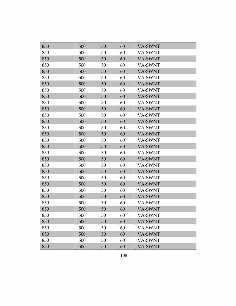
108
850 500 50 60 VA-SWNT
850 500 50 60 VA-SWNT
850 500 50 60 VA-SWNT
850 500 50 60 VA-SWNT
850 500 50 60 VA-SWNT
850 500 50 60 VA-SWNT
850 500 50 60 VA-SWNT
850 500 50 60 VA-SWNT
850 500 50 60 VA-SWNT
850 500 50 60 VA-SWNT
850 500 50 60 VA-SWNT
850 500 50 60 VA-SWNT
850 500 50 60 VA-SWNT
850 500 50 60 VA-SWNT
850 500 50 60 VA-SWNT
850 500 50 60 VA-SWNT
850 500 50 60 VA-SWNT
850 500 50 60 VA-SWNT
850 500 50 60 VA-SWNT
850 500 50 60 VA-SWNT
850 500 50 60 VA-SWNT
850 500 50 60 VA-SWNT
850 500 50 60 VA-SWNT
850 500 50 60 VA-SWNT
850 500 50 60 VA-SWNT
850 500 50 60 VA-SWNT
850 500 50 60 VA-SWNT
850 500 50 60 VA-SWNT
850 500 50 60 VA-SWNT
850 500 50 60 VA-SWNT
850 500 50 60 VA-SWNT
850 500 50 60 VA-SWNT
850 500 50 60 VA-SWNT

109
850 500 50 60 VA-SWNT
850 500 50 60 VA-SWNT
850 500 50 60 VA-SWNT
850 500 50 60 VA-SWNT
850 500 50 60 VA-SWNT
850 500 50 60 VA-SWNT
850 500 50 60 VA-SWNT
850 500 50 60 VA-SWNT
850 500 50 60 VA-SWNT
850 500 50 60 VA-SWNT
850 500 50 60 VA-SWNT
850 500 50 60 VA-SWNT
850 500 50 60 VA-SWNT
850 500 50 60 VA-SWNT
850 500 50 60 VA-SWNT
850 500 50 60 VA-SWNT
850 500 50 60 VA-SWNT
850 500 50 60 VA-SWNT
850 500 50 60 VA-SWNT
850 500 50 60 VA-SWNT
850 500 50 60 VA-SWNT
850 500 50 60 VA-SWNT
850 500 50 60 VA-SWNT
850 500 50 60 VA-SWNT
850 500 50 60 VA-SWNT
850 500 50 60 VA-SWNT
850 500 50 60 VA-SWNT
850 500 50 60 VA-SWNT
850 500 50 60 VA-SWNT
850 500 50 60 VA-SWNT
850 500 50 60 VA-SWNT
850 500 50 60 VA-SWNT
850 500 50 60 VA-SWNT

110
850 500 50 60 VA-SWNT
850 500 50 60 VA-SWNT
850 500 50 60 VA-SWNT
850 500 50 60 VA-SWNT
850 500 50 60 VA-SWNT
850 500 50 60 VA-SWNT
850 500 50 60 VA-SWNT
850 500 50 60 VA-SWNT
850 500 50 60 VA-SWNT
850 500 50 60 VA-SWNT
850 500 50 60 VA-SWNT
850 500 50 60 VA-SWNT
850 500 50 60 VA-SWNT
850 500 50 60 VA-SWNT
850 500 50 60 VA-SWNT
850 500 50 60 VA-SWNT
850 500 50 60 VA-SWNT
850 500 50 60 VA-SWNT
850 500 50 60 VA-SWNT
850 500 50 60 VA-SWNT
850 500 50 60 VA-SWNT
850 500 50 60 VA-SWNT
850 500 50 60 VA-SWNT
850 500 50 60 VA-SWNT
850 500 50 60 VA-SWNT
850 500 50 60 VA-SWNT
850 500 50 60 VA-SWNT
850 500 50 60 VA-SWNT
850 500 50 60 VA-SWNT
850 500 50 60 VA-SWNT
850 500 50 60 VA-SWNT
850 500 50 60 VA-SWNT
850 500 50 60 VA-SWNT

111
850 500 50 60 VA-SWNT
850 500 50 60 VA-SWNT
850 500 50 60 VA-SWNT
850 500 50 60 VA-SWNT
850 500 50 60 VA-SWNT
850 500 50 60 VA-SWNT
850 500 50 60 VA-SWNT
850 500 50 60 VA-SWNT
850 500 50 60 VA-SWNT
850 500 50 60 VA-SWNT
850 500 50 60 VA-SWNT
850 500 50 60 VA-SWNT
850 500 50 60 VA-SWNT
850 500 50 60 VA-SWNT
850 500 50 60 VA-SWNT
850 500 50 60 VA-SWNT
850 500 50 60 VA-SWNT
850 500 50 60 VA-SWNT
850 500 50 60 VA-SWNT
850 500 50 60 VA-SWNT
850 500 50 60 VA-SWNT
850 500 50 60 VA-SWNT
850 500 50 60 VA-SWNT
850 500 50 60 VA-SWNT
850 500 50 60 VA-SWNT
850 500 50 60 VA-SWNT
850 500 50 60 VA-SWNT
850 500 50 60 VA-SWNT
850 500 50 60 VA-SWNT
850 500 50 60 VA-SWNT
850 500 50 60 VA-SWNT
850 500 50 60 VA-SWNT
850 500 50 60 VA-SWNT

112
850 500 50 60 VA-SWNT
850 500 50 60 VA-SWNT
850 500 50 60 VA-SWNT
850 500 50 60 VA-SWNT
850 500 50 60 VA-SWNT
850 500 50 60 VA-SWNT
850 500 50 60 VA-SWNT
850 500 50 60 VA-SWNT
850 500 50 60 VA-SWNT
850 500 50 60 VA-SWNT
850 500 50 60 VA-SWNT
850 500 50 60 VA-SWNT
850 500 50 60 VA-SWNT
850 500 50 60 VA-SWNT
850 500 50 60 VA-SWNT
850 500 50 60 VA-SWNT
850 500 50 60 VA-SWNT
850 500 50 60 VA-SWNT
850 500 50 60 VA-SWNT
850 500 50 60 VA-SWNT
850 500 50 60 VA-SWNT
850 500 50 60 VA-SWNT
850 500 50 60 VA-SWNT
850 500 50 60 VA-SWNT
850 500 50 60 VA-SWNT
850 500 50 60 VA-SWNT
850 500 50 60 VA-SWNT
850 500 50 60 VA-SWNT
850 500 50 60 VA-SWNT
850 500 50 60 VA-SWNT
850 500 50 60 VA-SWNT
850 500 50 60 VA-SWNT
850 500 50 60 VA-SWNT

113
850 500 50 60 VA-SWNT
850 500 50 60 VA-SWNT
850 500 50 60 VA-SWNT
850 500 50 60 VA-SWNT
850 500 50 60 VA-SWNT
850 500 50 60 VA-SWNT
850 500 50 60 VA-SWNT
850 500 50 60 VA-SWNT
850 500 50 60 VA-SWNT
850 500 50 60 VA-SWNT
850 500 50 60 VA-SWNT
850 500 50 60 VA-SWNT
850 500 50 60 VA-SWNT
850 500 50 60 VA-SWNT
850 500 50 60 VA-SWNT
850 500 50 60 VA-SWNT
850 500 50 60 VA-SWNT
850 500 50 60 VA-SWNT
850 500 50 60 VA-SWNT
850 500 50 60 VA-SWNT
850 500 50 60 VA-SWNT
850 500 50 60 VA-SWNT
850 500 50 60 VA-SWNT
850 500 50 60 VA-SWNT
850 500 50 60 VA-SWNT
890 700 75 40 VA-SWNT
890 700 75 40 VA-SWNT
890 700 75 40 VA-SWNT
890 700 75 40 VA-SWNT
890 700 75 40 VA-SWNT
890 756 400 30 VA-SWNT
890 700 400 30 VA-SWNT
890 700 400 30 VA-SWNT
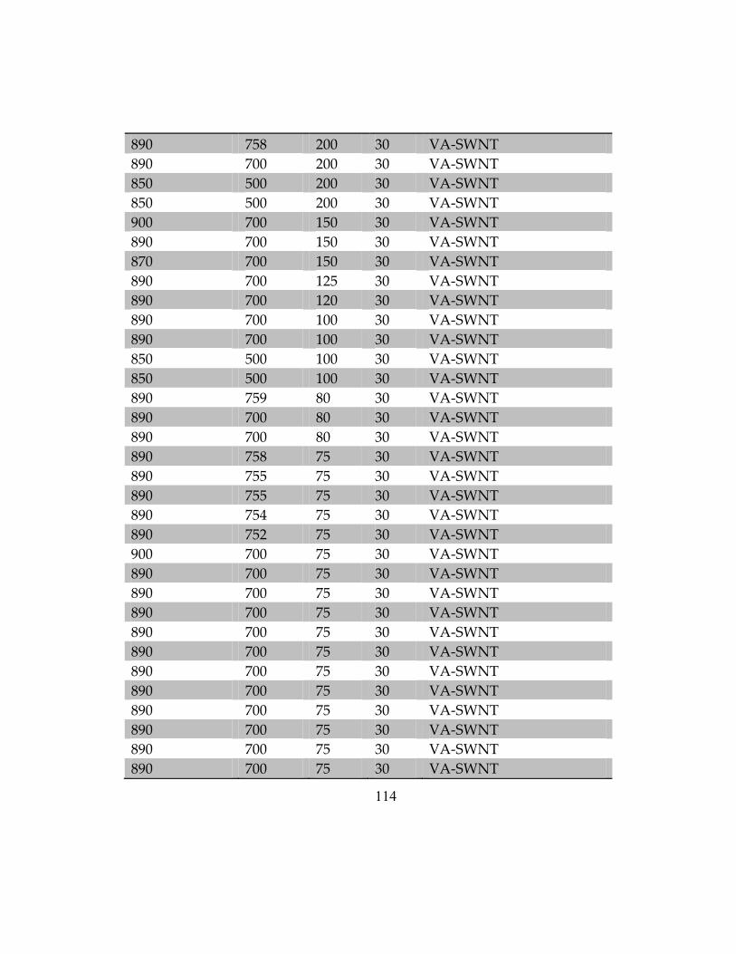
114
890 758 200 30 VA-SWNT
890 700 200 30 VA-SWNT
850 500 200 30 VA-SWNT
850 500 200 30 VA-SWNT
900 700 150 30 VA-SWNT
890 700 150 30 VA-SWNT
870 700 150 30 VA-SWNT
890 700 125 30 VA-SWNT
890 700 120 30 VA-SWNT
890 700 100 30 VA-SWNT
890 700 100 30 VA-SWNT
850 500 100 30 VA-SWNT
850 500 100 30 VA-SWNT
890 759 80 30 VA-SWNT
890 700 80 30 VA-SWNT
890 700 80 30 VA-SWNT
890 758 75 30 VA-SWNT
890 755 75 30 VA-SWNT
890 755 75 30 VA-SWNT
890 754 75 30 VA-SWNT
890 752 75 30 VA-SWNT
900 700 75 30 VA-SWNT
890 700 75 30 VA-SWNT
890 700 75 30 VA-SWNT
890 700 75 30 VA-SWNT
890 700 75 30 VA-SWNT
890 700 75 30 VA-SWNT
890 700 75 30 VA-SWNT
890 700 75 30 VA-SWNT
890 700 75 30 VA-SWNT
890 700 75 30 VA-SWNT
890 700 75 30 VA-SWNT
890 700 75 30 VA-SWNT

115
880 700 75 30 VA-SWNT
880 700 75 30 VA-SWNT
880 700 75 30 VA-SWNT
890 700 50 30 VA-SWNT
890 700 50 30 VA-SWNT
890 700 50 30 VA-SWNT
890 700 50 30 VA-SWNT
850 500 50 30 VA-SWNT
850 500 50 30 VA-SWNT
850 500 50 30 VA-SWNT
850 500 50 30 VA-SWNT
850 500 50 30 VA-SWNT
850 500 50 30 VA-SWNT
850 500 50 30 VA-SWNT
850 500 50 30 VA-SWNT
850 500 50 30 VA-SWNT
850 500 50 30 VA-SWNT
850 500 50 30 VA-SWNT
850 500 50 30 VA-SWNT
850 500 50 30 VA-SWNT
850 500 50 30 VA-SWNT
850 500 50 30 VA-SWNT
850 500 50 30 VA-SWNT
850 500 50 30 VA-SWNT
850 500 50 30 VA-SWNT
850 500 50 30 VA-SWNT
850 500 50 30 VA-SWNT
850 500 50 30 VA-SWNT
850 500 50 30 VA-SWNT
850 500 50 30 VA-SWNT
850 500 50 30 VA-SWNT
850 500 50 30 VA-SWNT
850 500 50 30 VA-SWNT

116
850 500 50 30 VA-SWNT
850 500 50 30 VA-SWNT
850 500 50 30 VA-SWNT
850 500 50 30 VA-SWNT
850 500 50 30 VA-SWNT
850 500 50 30 VA-SWNT
850 500 50 30 VA-SWNT
850 500 50 30 VA-SWNT
850 500 50 30 VA-SWNT
850 500 50 30 VA-SWNT
850 500 50 30 VA-SWNT
850 500 50 30 VA-SWNT
850 500 50 30 VA-SWNT
850 500 50 30 VA-SWNT
850 500 50 30 VA-SWNT
850 500 50 30 VA-SWNT
890 754 75 25 VA-SWNT
1000 500 400 30 Small amount of MWNT
1000 500 400 30 Small amount of MWNT
900 500 400 30 Small amount of MWNT
900 500 400 30 Small amount of MWNT
850 500 400 30 Small amount of MWNT
850 500 400 30 Small amount of MWNT
850 500 400 30 Small amount of MWNT
800 500 400 30 Small amount of MWNT
800 500 400 30 Small amount of MWNT
800 500 400 30 Small amount of MWNT
750 500 400 30 Small amount of MWNT
750 500 400 30 Small amount of MWNT
750 500 400 30 Small amount of MWNT
700 500 400 30 Small amount of MWNT
700 500 400 30 Small amount of MWNT
700 500 400 30 Small amount of MWNT

117
700 500 400 30 Small amount of MWNT
1000 500 300 30 Small amount of MWNT
1000 500 300 30 Small amount of MWNT
1000 500 300 30 Small amount of MWNT
900 500 300 30 Small amount of MWNT
900 500 300 30 Small amount of MWNT
900 500 300 30 Small amount of MWNT
850 500 300 30 Small amount of MWNT
850 500 300 30 Small amount of MWNT
850 500 300 30 Small amount of MWNT
800 500 300 30 Small amount of MWNT
800 500 300 30 Small amount of MWNT
800 500 300 30 Small amount of MWNT
750 500 300 30 Small amount of MWNT
750 500 300 30 Small amount of MWNT
750 500 300 30 Small amount of MWNT
700 500 300 30 Small amount of MWNT
700 500 300 30 Small amount of MWNT
700 500 300 30 Small amount of MWNT
700 500 300 30 Small amount of MWNT
700 500 300 30 Small amount of MWNT
1000 500 200 30 Small amount of MWNT
1000 500 200 30 Small amount of MWNT
1000 500 200 30 Small amount of MWNT
900 500 200 30 Small amount of MWNT
900 500 200 30 Small amount of MWNT
900 500 200 30 Small amount of MWNT
850 500 200 30 Small amount of MWNT
850 500 200 30 Small amount of MWNT
850 500 200 30 Small amount of MWNT
800 500 200 30 Small amount of MWNT
800 500 200 30 Small amount of MWNT
800 500 200 30 Small amount of MWNT

118
750 500 200 30 Small amount of MWNT
750 500 200 30 Small amount of MWNT
750 500 200 30 Small amount of MWNT
700 500 200 30 Small amount of MWNT
700 500 200 30 Small amount of MWNT
700 500 200 30 Small amount of MWNT
700 500 200 30 Small amount of MWNT
700 500 200 30 Small amount of MWNT
700 500 200 30 Small amount of MWNT
1000 500 100 30 Small amount of MWNT
1000 500 100 30 Small amount of MWNT
1000 500 100 30 Small amount of MWNT
900 500 100 30 Small amount of MWNT
900 500 100 30 Small amount of MWNT
900 500 100 30 Small amount of MWNT
850 500 100 30 Small amount of MWNT
850 500 100 30 Small amount of MWNT
850 500 100 30 Small amount of MWNT
800 500 100 30 Small amount of MWNT
800 500 100 30 Small amount of MWNT
800 500 100 30 Small amount of MWNT
750 500 100 30 Small amount of MWNT
750 500 100 30 Small amount of MWNT
750 500 100 30 Small amount of MWNT
700 500 100 30 Small amount of MWNT
700 500 100 30 Small amount of MWNT
700 500 100 30 Small amount of MWNT
700 500 100 30 Small amount of MWNT
1000 500 50 30 Small amount of MWNT
1000 500 50 30 Small amount of MWNT
1000 500 50 30 Small amount of MWNT
900 500 50 30 Small amount of MWNT
900 500 50 30 Small amount of MWNT
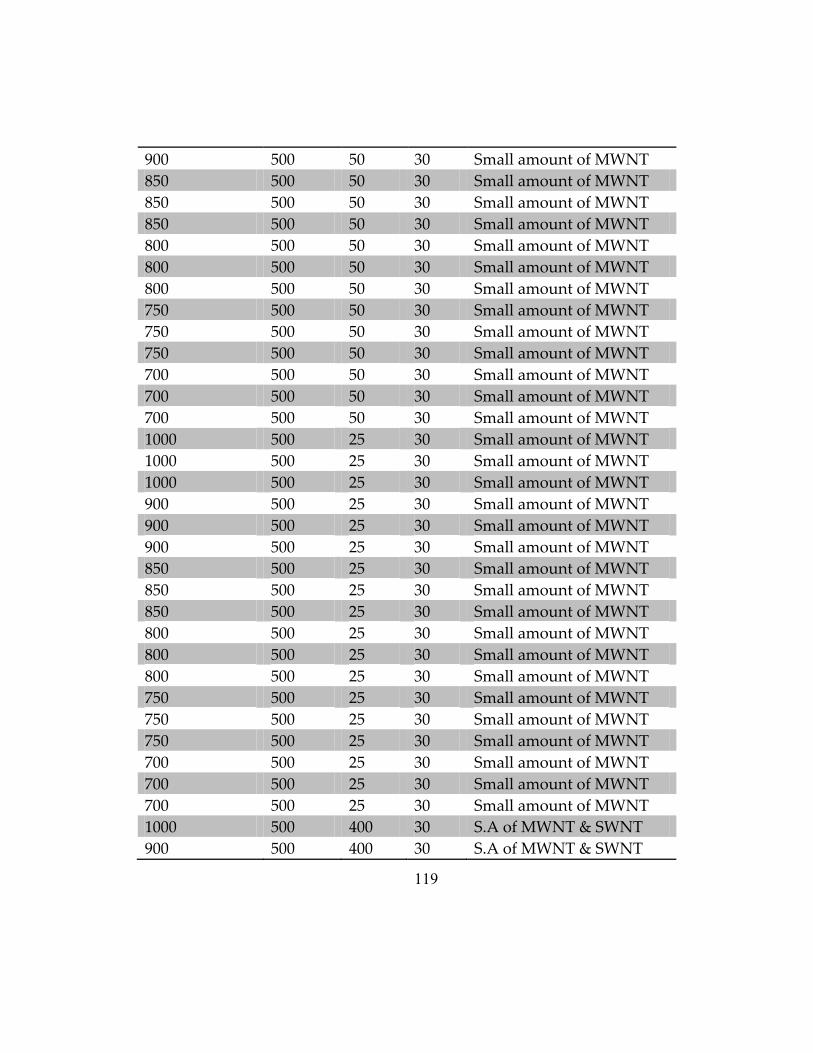
119
900 500 50 30 Small amount of MWNT
850 500 50 30 Small amount of MWNT
850 500 50 30 Small amount of MWNT
850 500 50 30 Small amount of MWNT
800 500 50 30 Small amount of MWNT
800 500 50 30 Small amount of MWNT
800 500 50 30 Small amount of MWNT
750 500 50 30 Small amount of MWNT
750 500 50 30 Small amount of MWNT
750 500 50 30 Small amount of MWNT
700 500 50 30 Small amount of MWNT
700 500 50 30 Small amount of MWNT
700 500 50 30 Small amount of MWNT
1000 500 25 30 Small amount of MWNT
1000 500 25 30 Small amount of MWNT
1000 500 25 30 Small amount of MWNT
900 500 25 30 Small amount of MWNT
900 500 25 30 Small amount of MWNT
900 500 25 30 Small amount of MWNT
850 500 25 30 Small amount of MWNT
850 500 25 30 Small amount of MWNT
850 500 25 30 Small amount of MWNT
800 500 25 30 Small amount of MWNT
800 500 25 30 Small amount of MWNT
800 500 25 30 Small amount of MWNT
750 500 25 30 Small amount of MWNT
750 500 25 30 Small amount of MWNT
750 500 25 30 Small amount of MWNT
700 500 25 30 Small amount of MWNT
700 500 25 30 Small amount of MWNT
700 500 25 30 Small amount of MWNT
1000 500 400 30 S.A of MWNT & SWNT
900 500 400 30 S.A of MWNT & SWNT

120
850 500 400 30 S.A of MWNT & SWNT
800 500 400 30 S.A of MWNT & SWNT
750 500 400 30 S.A of MWNT & SWNT
1000 500 300 30 S.A of MWNT & SWNT
900 500 300 30 S.A of MWNT & SWNT
850 500 300 30 S.A of MWNT & SWNT
800 500 300 30 S.A of MWNT & SWNT
750 500 300 30 S.A of MWNT & SWNT
1000 500 200 30 S.A of MWNT & SWNT
900 500 200 30 S.A of MWNT & SWNT
850 500 200 30 S.A of MWNT & SWNT
800 500 200 30 S.A of MWNT & SWNT
750 500 200 30 S.A of MWNT & SWNT
700 500 200 30 S.A of MWNT & SWNT
1000 500 100 30 S.A of MWNT & SWNT
900 500 100 30 S.A of MWNT & SWNT
850 500 100 30 S.A of MWNT & SWNT
800 500 100 30 S.A of MWNT & SWNT
750 500 100 30 S.A of MWNT & SWNT
700 500 100 30 S.A of MWNT & SWNT
1000 500 50 30 S.A of MWNT & SWNT
900 500 50 30 S.A of MWNT & SWNT
850 500 50 30 S.A of MWNT & SWNT
800 500 50 30 S.A of MWNT & SWNT
750 500 50 30 S.A of MWNT & SWNT
700 500 50 30 S.A of MWNT & SWNT
1000 500 25 30 S.A of MWNT & SWNT
900 500 25 30 S.A of MWNT & SWNT
850 500 25 30 S.A of MWNT & SWNT
800 500 25 30 S.A of MWNT & SWNT
750 500 25 30 S.A of MWNT & SWNT
700 500 25 30 S.A of MWNT & SWNT
890 755 200 60 none

121
850 500 200 60 none
850 500 200 60 none
890 700 100 60 none
890 764 80 60 none
890 763 80 60 none
850 500 50 60 none
850 500 50 60 none
850 500 50 60 none
850 500 50 60 none
850 500 50 60 none
850 500 50 60 none
850 500 50 60 none
850 500 50 60 none
850 500 50 60 none
850 500 50 60 none
850 500 50 60 none
850 500 50 60 none
850 500 50 60 none
850 500 50 60 none
850 500 50 60 none
850 500 50 60 none
850 500 50 60 none
850 500 50 60 none
850 500 50 60 none
850 500 50 60 none
850 500 50 60 none
850 500 50 60 none
850 500 50 60 none
850 500 50 60 none
850 500 50 60 none
850 500 50 60 none
850 500 50 60 none
850 500 50 60 none

122
850 500 50 60 none
850 500 50 60 none
850 500 50 60 none
850 500 50 60 none
850 500 500 30 none
850 500 500 30 none
850 500 400 30 none
850 500 400 30 none
750 500 400 30 none
700 500 400 30 none
850 500 300 30 none
850 500 300 30 none
700 500 300 30 none
850 500 200 30 none
850 500 200 30 none
900 500 100 30 none
900 500 100 30 none
850 500 100 30 none
850 500 100 30 none
850 500 100 30 none
850 500 100 30 none
800 500 100 30 none
800 500 100 30 none
750 500 100 30 none
750 500 100 30 none
750 500 100 30 none
750 500 100 30 none
700 500 100 30 none
700 500 100 30 none
700 500 100 30 none
890 754 75 30 none
850 500 50 30 none
850 500 50 30 none

123
850 500 50 30 none
850 500 50 30 none
850 500 50 30 none
850 500 50 30 none
850 500 50 30 none
850 500 50 30 none
850 500 50 30 none
850 500 50 30 none
850 500 50 30 none
850 500 50 30 none
850 500 50 30 none
850 500 50 30 none
850 500 50 30 none
850 500 50 30 none
850 500 50 30 none
850 500 50 30 none
DOE Data
Temperature Pressure Flow Time Result
700 500 50 250 none
700 500 50 420 S.A of MWNT & SWNT
700 500 50 600 none
700 500 225 250 Small amount of MWNT
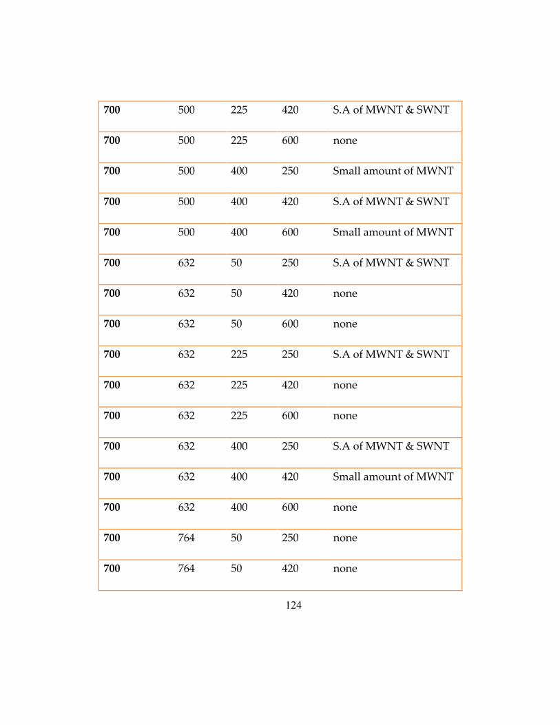
124
700 500 225 420 S.A of MWNT & SWNT
700 500 225 600 none
700 500 400 250 Small amount of MWNT
700 500 400 420 S.A of MWNT & SWNT
700 500 400 600 Small amount of MWNT
700 632 50 250 S.A of MWNT & SWNT
700 632 50 420 none
700 632 50 600 none
700 632 225 250 S.A of MWNT & SWNT
700 632 225 420 none
700 632 225 600 none
700 632 400 250 S.A of MWNT & SWNT
700 632 400 420 Small amount of MWNT
700 632 400 600 none
700 764 50 250 none
700 764 50 420 none

125
700 764 50 600 none
700 764 225 250 none
700 764 225 420 none
700 764 225 600 none
700 764 400 250 none
700 764 400 420 none
700 764 400 600 none
800 500 50 250 Small amount of MWNT
800 500 50 420 S.A of MWNT & SWNT
800 500 50 600 none
800 500 225 250 Small amount of MWNT
800 500 225 420 S.A of MWNT & SWNT
800 500 225 600 none
800 500 400 250 Small amount of MWNT
800 500 400 420 S.A of MWNT & SWNT
800 500 400 600 S.A of MWNT & SWNT
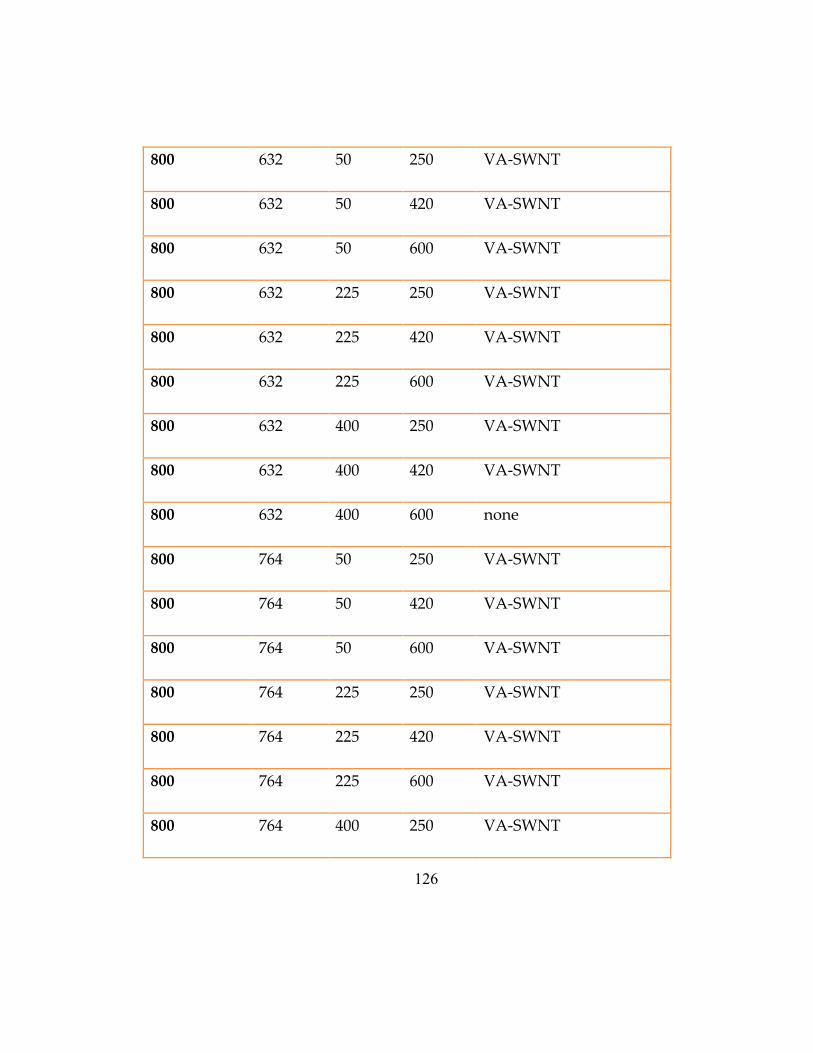
126
800 632 50 250 VA-SWNT
800 632 50 420 VA-SWNT
800 632 50 600 VA-SWNT
800 632 225 250 VA-SWNT
800 632 225 420 VA-SWNT
800 632 225 600 VA-SWNT
800 632 400 250 VA-SWNT
800 632 400 420 VA-SWNT
800 632 400 600 none
800 764 50 250 VA-SWNT
800 764 50 420 VA-SWNT
800 764 50 600 VA-SWNT
800 764 225 250 VA-SWNT
800 764 225 420 VA-SWNT
800 764 225 600 VA-SWNT
800 764 400 250 VA-SWNT

127
800 764 400 420 VA-SWNT
800 764 400 600 VA-SWNT
900 500 50 250 none
900 500 50 420 VA-SWNT
900 500 50 600 VA-SWNT
900 500 225 250 Small amount of MWNT
900 500 225 420 S.A of MWNT & SWNT
900 500 225 600 VA-SWNT
900 500 400 250 none
900 500 400 420 S.A of MWNT & SWNT
900 500 400 600 VA-SWNT
900 632 50 250 VA-SWNT
900 632 50 420 VA-SWNT
900 632 50 600 VA-SWNT
900 632 225 250 VA-SWNT
900 632 225 420 VA-SWNT

128
900 632 225 600 VA-SWNT
900 632 400 250 VA-SWNT
900 632 400 420 VA-SWNT
900 632 400 600 VA-SWNT
900 764 50 250 VA-SWNT
900 764 50 420 VA-SWNT
900 764 50 600 VA-SWNT
900 764 225 250 VA-SWNT
900 764 225 420 VA-SWNT
900 764 225 600 VA-SWNT
900 764 400 250 VA-SWNT
900 764 400 420 VA-SWNT
900 764 400 600 VA-SWNT
C Source File
//Analysis Type - Classification

129
#include <stdio.h>
#include <conio.h>
#include <math.h>
#include <stdlib.h>
double input_hidden_weights[12][4]=
{
{-1.10626389895333e+000, -3.73643496006291e-003, 5.96566965299829e+000,
2.12499984937343e+000 },
{6.57731612579698e-001, -2.92481134061285e+000, -7.85101897381701e-001,
1.64231401512658e+000 },
{-1.16058873730090e+001, -8.92886691018749e+000, 5.43316705908870e+000, -
4.83392243846306e+000 },
{-5.21276960171781e+000, -6.62498586125943e-001, -2.53690312098249e+000,
5.80096137446396e-001 },
{1.95455434574576e-001, 2.27916688256394e+000, 1.95448650355832e+000,
1.07630239317822e+000 },
{3.16576736733244e+000, -4.14960880259401e+000, -4.92500806780292e+000, -
3.48665624799860e+000 },
{8.74702498089894e+000, -4.58648936262645e+000, -2.26116853452984e+000, -
1.11784635782786e+000 },
{1.04861692985922e+000, -4.30718908920277e+000, -1.45599407693833e+000, -
3.83921115266548e+000 },
{1.20344648378913e+000, 4.91528926944447e+000, -1.35668049826802e+000, -
1.45964626930918e+000 },
{-1.40925587887915e+000, -3.73382786683886e+000, -2.07472417539196e+001, -
3.05847487083543e+000 },

130
{2.89719585458340e-001, -2.86859795404039e+000, -7.99821806345248e-001,
3.14126157045974e-001 },
{2.57779598097478e+000, -3.70422470781917e+000, -4.13173188587870e+000, -
7.20501918350059e-001 }
};
double hidden_bias[12]={ -3.98566483194604e+000, -9.43831760189939e-001,
5.17789669494765e+000, 9.65571074908640e-001, -5.69755420045899e-001, -
3.74927386846146e-001, -3.41779205020830e+000, -7.12520353454542e-001, -
1.07829605709090e+000, 2.65972689551957e+000, 1.71014648061759e-001, -
9.25008699698261e-002 };
double hidden_output_wts[4][12]=
{
{3.79361473524166e-001, -4.42293097221627e+000, -6.95536471294875e-004, -
6.26475374686074e-001, -1.12462198943676e+000, 3.09203595031522e-001,
3.77856184512851e-002, 1.27552964135618e+000, -1.75567973130942e+000,
1.73495548739488e-001, -1.99319110089557e+000, -6.59944854194473e-001 },
{-4.94462713236383e-001, -4.10065790869239e+000, 1.18290472182240e-004, -
1.47770701847982e-001, 2.89119115325853e-001, -2.02500595416126e-001,
2.22915702640809e-002, 3.85382053492280e+000, -4.13326836232414e+000,
1.14046369358423e-001, 3.73791241241672e-001, 4.94510325402918e-002 },
{1.62526284591701e-001, 4.69852312118827e-002, -5.33852531663558e+000, -
6.68527743098429e-002, -9.28439519529504e-003, 3.37202788325939e+000, -
2.29854749015291e+000, 2.73951374354158e+000, -2.90720424550613e-003, -
1.76806579230098e+000, 1.54873415426241e-001, 8.31978976118578e-001 },
{5.00692372344648e-002, 6.92434479070777e-001, -2.31526502993601e-002,
4.16740293309858e+000, 7.02582997480717e-001, 2.03961158903557e+000, -
9.80452572039321e-001, -1.43400429584647e-001, -2.10235980310695e+000, -
2.17975138935412e+000, -6.14022135063163e+000, 2.80423145063388e+000 }
};

131
double output_bias[4]={ 4.80480210266358e+000, 6.83717178164568e-001,
9.78925664392187e-002, 1.50652260101541e+000 };
double max_input[4]={ 10000000000e+003, 7.64000000000000e+002,
50000000000e+002, 60000000000e+001 };
double min_input[4]={ 70000000000e+002, 50000000000e+002,
2.50000000000000e+001, 2.50000000000000e+001 };
double input[4];
double hidden[12];
double output[4];
void ScaleInputs(double* input, double minimum, double maximum, int size)
{
double delta;
long i;
for(i=0; i<size; i++)
{
delta = (maximum-minimum)/(max_input[i]-min_input[i]);
input[i] = minimum - delta*min_input[i]+ delta*input[i];
}
}
void ComputeFeedForwardSignals(double* MAT_INOUT,double*
V_IN,double* V_OUT, double* V_BIAS,int size1,int size2,int layer)
{
int row,col;
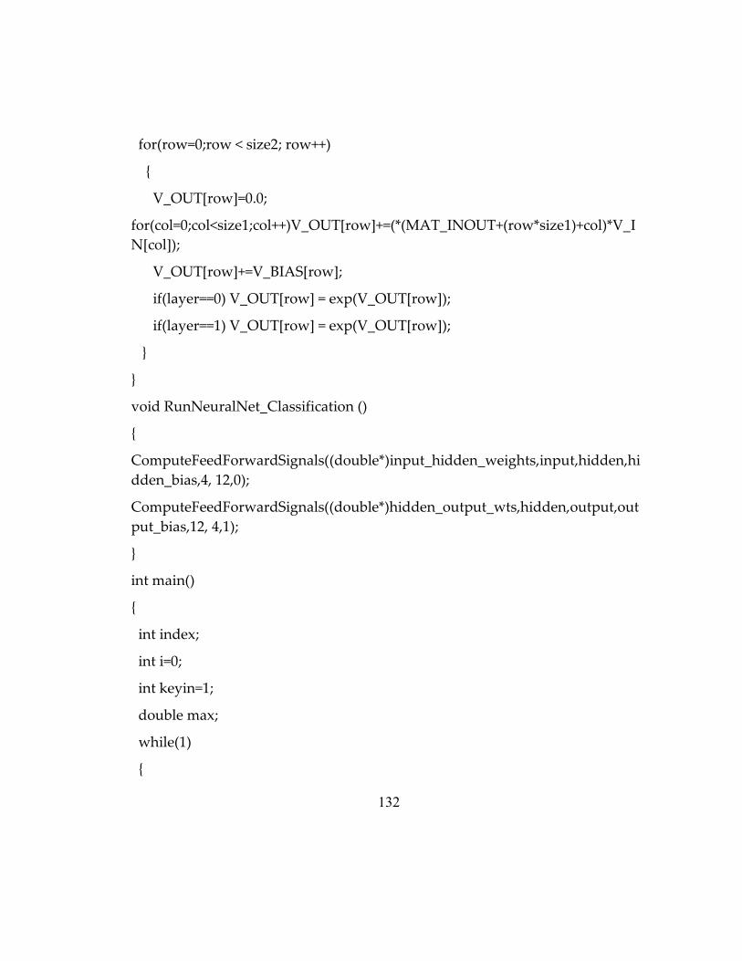
132
for(row=0;row < size2; row++)
{
V_OUT[row]=0.0;
for(col=0;col<size1;col++)V_OUT[row]+=(*(MAT_INOUT+(row*size1)+col)*V_I
N[col]);
V_OUT[row]+=V_BIAS[row];
if(layer==0) V_OUT[row] = exp(V_OUT[row]);
if(layer==1) V_OUT[row] = exp(V_OUT[row]);
}
}
void RunNeuralNet_Classification ()
{
ComputeFeedForwardSignals((double*)input_hidden_weights,input,hidden,hi
dden_bias,4, 12,0);
ComputeFeedForwardSignals((double*)hidden_output_wts,hidden,output,out
put_bias,12, 4,1);
}
int main()
{
int index;
int i=0;
int keyin=1;
double max;
while(1)
{

133
max=3.e-300;
printf("\nEnter values for Continuous inputs\n");
printf("Cont. Input-0(Temperature (°C)): ");
scanf("%lg",&input[0]);
printf("Cont. Input-1(Pressure (torr)): ");
scanf("%lg",&input[1]);
printf("Cont. Input-2(Flow Rate (sccm)): ");
scanf("%lg",&input[2]);
printf("Cont. Input-3(Time (min)): ");
scanf("%lg",&input[3]);
ScaleInputs(input,0,1,4);
RunNeuralNet_Classification();
for(i=0;i<4;i++)
{
if(max<output[i])
{
max=output[i];
index=i+1;
}
}
printf("\nPredicted category = ");
switch(index)
{

134
case 1: printf("S.A of MWNT & SWNT\n"); break;
case 2: printf("Small amount of MWNT\n"); break;
case 3: printf("VA-SWNT\n"); break;
case 4: printf("none\n"); break;
default: break;
}
printf("\nConfidence level = %.14f",max);
printf("\n\nPress any key to make another prediction or enter 0 to quit
the program.\n");
keyin=getch();
if(keyin==48)break;
}
return 0;
}
XML Document
<?xml version="1.0" encoding="UTF-8"?>
<PMML version="3.0"><Header copyright="Copyright (c) StatSoft, Inc. All
Rights Reserved."><Application name="STATISTICA Automated Neural
Networks (SANN)" version="2.0"/></Header><DataDictionary
numberOfFields="5"><DataField name="Result" optype="categorical"><Value
value="S.A of MWNT & SWNT"/><Value value="Small amount of
MWNT"/><Value value="VA-SWNT"/><Value
value="none"/></DataField><DataField name="Temperature (°C)"
optype="continuous"/><DataField name="Pressure (torr)"
optype="continuous"/><DataField name="Flow Rate (sccm)"
optype="continuous"/><DataField name="Time (min)"

135
optype="continuous"/></DataDictionary><NeuralNetwork modelName="Book1
c_MLP 4-12-4" functionName="classification"><MiningSchema><MiningField
name="Result" usageType="predicted"/><MiningField name="Temperature
(°C)" lowValue="70000" highValue="100000"/><MiningField name="Pressure
(torr)" lowValue="50000" highValue="76400"/><MiningField name="Flow Rate
(sccm)" lowValue="2500" highValue="50000"/><MiningField name="Time (min)"
lowValue="2500" highValue="6000"/></MiningSchema><NeuralInputs
numberOfInputs="4"><NeuralInput id="0"><DerivedField><NormContinuous
field="Temperature (°C)"><LinearNorm orig="70000000000e+002"
norm="000"/><LinearNorm orig="10000000000e+003"
norm="100"/></NormContinuous></DerivedField></NeuralInput><NeuralInput
id="1"><DerivedField><NormContinuous field="Pressure (torr)"><LinearNorm
orig="50000000000e+002" norm="000"/><LinearNorm
orig="7.64000000000000e+002"
norm="100"/></NormContinuous></DerivedField></NeuralInput><NeuralInput
id="2"><DerivedField><NormContinuous field="Flow Rate
(sccm)"><LinearNorm orig="2.50000000000000e+001"
norm="000"/><LinearNorm orig="50000000000e+002"
norm="100"/></NormContinuous></DerivedField></NeuralInput><NeuralInput
id="3"><DerivedField><NormContinuous field="Time (min)"><LinearNorm
orig="2.50000000000000e+001" norm="000"/><LinearNorm
orig="60000000000e+001"
norm="100"/></NormContinuous></DerivedField></NeuralInput></NeuralInpu
ts><NeuralLayer numberOfNeurons="12"
activationFunction="exponential"><Neuron id="4" bias="-
3.98566483194604e+000"><Con from="0" weight="-
1.10626389895333e+000"/><Con from="1" weight="-3.73643496006291e-
003"/><Con from="2" weight="5.96566965299829e+000"/><Con from="3"
weight="2.12499984937343e+000"/></Neuron><Neuron id="5" bias="-
9.43831760189939e-001"><Con from="0" weight="6.57731612579698e-001"/><Con
from="1" weight="-2.92481134061285e+000"/><Con from="2" weight="-
7.85101897381701e-001"/><Con from="3"
weight="1.64231401512658e+000"/></Neuron><Neuron id="6"

136
bias="5.17789669494765e+000"><Con from="0" weight="-
1.16058873730090e+001"/><Con from="1" weight="-
8.92886691018749e+000"/><Con from="2"
weight="5.43316705908870e+000"/><Con from="3" weight="-
4.83392243846306e+000"/></Neuron><Neuron id="7" bias="9.65571074908640e-
001"><Con from="0" weight="-5.21276960171781e+000"/><Con from="1"
weight="-6.62498586125943e-001"/><Con from="2" weight="-
2.53690312098249e+000"/><Con from="3" weight="5.80096137446396e-
001"/></Neuron><Neuron id="8" bias="-5.69755420045899e-001"><Con from="0"
weight="1.95455434574576e-001"/><Con from="1"
weight="2.27916688256394e+000"/><Con from="2"
weight="1.95448650355832e+000"/><Con from="3"
weight="1.07630239317822e+000"/></Neuron><Neuron id="9" bias="-
3.74927386846146e-001"><Con from="0" weight="3.16576736733244e+000"/><Con
from="1" weight="-4.14960880259401e+000"/><Con from="2" weight="-
4.92500806780292e+000"/><Con from="3" weight="-
3.48665624799860e+000"/></Neuron><Neuron id="10" bias="-
3.41779205020830e+000"><Con from="0"
weight="8.74702498089894e+000"/><Con from="1" weight="-
4.58648936262645e+000"/><Con from="2" weight="-
2.26116853452984e+000"/><Con from="3" weight="-
1.11784635782786e+000"/></Neuron><Neuron id="11" bias="-7.12520353454542e-
001"><Con from="0" weight="1.04861692985922e+000"/><Con from="1"
weight="-4.30718908920277e+000"/><Con from="2" weight="-
1.45599407693833e+000"/><Con from="3" weight="-
3.83921115266548e+000"/></Neuron><Neuron id="12" bias="-
1.07829605709090e+000"><Con from="0"
weight="1.20344648378913e+000"/><Con from="1"
weight="4.91528926944447e+000"/><Con from="2" weight="-
1.35668049826802e+000"/><Con from="3" weight="-
1.45964626930918e+000"/></Neuron><Neuron id="13"
bias="2.65972689551957e+000"><Con from="0" weight="-
1.40925587887915e+000"/><Con from="1" weight="-

137
3.73382786683886e+000"/><Con from="2" weight="-
2.07472417539196e+001"/><Con from="3" weight="-
3.05847487083543e+000"/></Neuron><Neuron id="14" bias="1.71014648061759e-
001"><Con from="0" weight="2.89719585458340e-001"/><Con from="1" weight="-
2.86859795404039e+000"/><Con from="2" weight="-7.99821806345248e-
001"/><Con from="3" weight="3.14126157045974e-001"/></Neuron><Neuron
id="15" bias="-9.25008699698261e-002"><Con from="0"
weight="2.57779598097478e+000"/><Con from="1" weight="-
3.70422470781917e+000"/><Con from="2" weight="-
4.13173188587870e+000"/><Con from="3" weight="-7.20501918350059e-
001"/></Neuron></NeuralLayer><NeuralLayer numberOfNeurons="4"
activationFunction="exponential"><Neuron id="16"
bias="4.80480210266358e+000"><Con from="4" weight="3.79361473524166e-
001"/><Con from="5" weight="-4.42293097221627e+000"/><Con from="6"
weight="-6.95536471294875e-004"/><Con from="7" weight="-6.26475374686074e-
001"/><Con from="8" weight="-1.12462198943676e+000"/><Con from="9"
weight="3.09203595031522e-001"/><Con from="10" weight="3.77856184512851e-
002"/><Con from="11" weight="1.27552964135618e+000"/><Con from="12"
weight="-1.75567973130942e+000"/><Con from="13"
weight="1.73495548739488e-001"/><Con from="14" weight="-
1.99319110089557e+000"/><Con from="15" weight="-6.59944854194473e-
001"/></Neuron><Neuron id="17" bias="6.83717178164568e-001"><Con from="4"
weight="-4.94462713236383e-001"/><Con from="5" weight="-
4.10065790869239e+000"/><Con from="6" weight="1.18290472182240e-
004"/><Con from="7" weight="-1.47770701847982e-001"/><Con from="8"
weight="2.89119115325853e-001"/><Con from="9" weight="-2.02500595416126e-
001"/><Con from="10" weight="2.22915702640809e-002"/><Con from="11"
weight="3.85382053492280e+000"/><Con from="12" weight="-
4.13326836232414e+000"/><Con from="13" weight="1.14046369358423e-
001"/><Con from="14" weight="3.73791241241672e-001"/><Con from="15"
weight="4.94510325402918e-002"/></Neuron><Neuron id="18"
bias="9.78925664392187e-002"><Con from="4" weight="1.62526284591701e-
001"/><Con from="5" weight="4.69852312118827e-002"/><Con from="6"

138
weight="-5.33852531663558e+000"/><Con from="7" weight="-6.68527743098429e-
002"/><Con from="8" weight="-9.28439519529504e-003"/><Con from="9"
weight="3.37202788325939e+000"/><Con from="10" weight="-
2.29854749015291e+000"/><Con from="11"
weight="2.73951374354158e+000"/><Con from="12" weight="-
2.90720424550613e-003"/><Con from="13" weight="-
1.76806579230098e+000"/><Con from="14" weight="1.54873415426241e-
001"/><Con from="15" weight="8.31978976118578e-001"/></Neuron><Neuron
id="19" bias="1.50652260101541e+000"><Con from="4"
weight="5.00692372344648e-002"/><Con from="5" weight="6.92434479070777e-
001"/><Con from="6" weight="-2.31526502993601e-002"/><Con from="7"
weight="4.16740293309858e+000"/><Con from="8" weight="7.02582997480717e-
001"/><Con from="9" weight="2.03961158903557e+000"/><Con from="10"
weight="-9.80452572039321e-001"/><Con from="11" weight="-
1.43400429584647e-001"/><Con from="12" weight="-
2.10235980310695e+000"/><Con from="13" weight="-
2.17975138935412e+000"/><Con from="14" weight="-
6.14022135063163e+000"/><Con from="15"
weight="2.80423145063388e+000"/></Neuron></NeuralLayer><NeuralOutputs
numberOfOutputs="4"><NeuralOutput outputNeuron="16"><DerivedField
optype="categorical"><NormDiscrete field="Result" value="S.A of MWNT
& SWNT"/></DerivedField></NeuralOutput><NeuralOutput
outputNeuron="17"><DerivedField optype="categorical"><NormDiscrete
field="Result" value="Small amount of
MWNT"/></DerivedField></NeuralOutput><NeuralOutput
outputNeuron="18"><DerivedField optype="categorical"><NormDiscrete
field="Result" value="VA-
SWNT"/></DerivedField></NeuralOutput><NeuralOutput
outputNeuron="19"><DerivedField optype="categorical"><NormDiscrete
field="Result"
value="none"/></DerivedField></NeuralOutput></NeuralOutputs></NeuralNet
work></PMML>

139
Appendix C
Experimental Data
Temp. P (torr) Flow (sccm) time (min) length
870 700 150 30 900
880 700 75 30 150
880 700 75 30 150
880 700 75 30 500
890 700 100 60 0
890 754 75 30 0
890 755 200 60 0
890 763 80 60 0
890 764 80 60 0
890 700 75 30 100
890 700 400 30 100
890 700 400 30 100
890 700 75 40 100
890 700 75 60 100
890 752 75 60 100
890 754 75 25 100
890 758 75 30 100
890 759 80 30 100
890 759 80 60 100
890 700 50 30 150
890 700 50 30 150
890 700 75 30 150
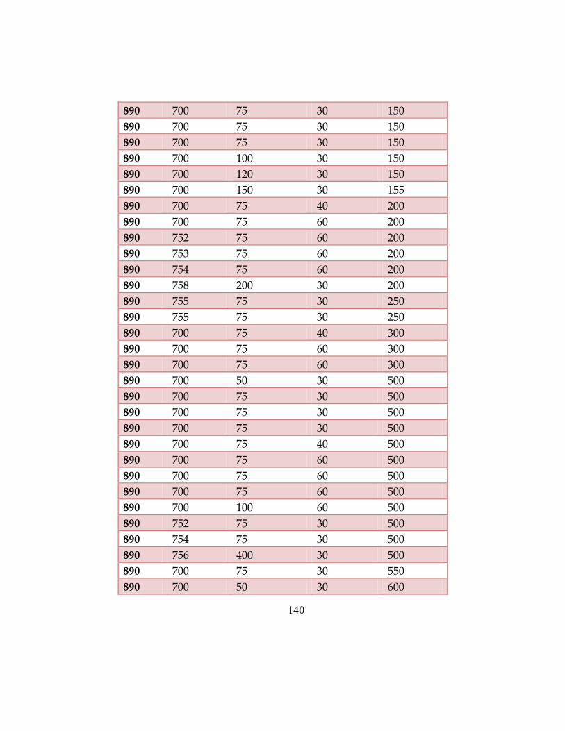
140
890 700 75 30 150
890 700 75 30 150
890 700 75 30 150
890 700 100 30 150
890 700 120 30 150
890 700 150 30 155
890 700 75 40 200
890 700 75 60 200
890 752 75 60 200
890 753 75 60 200
890 754 75 60 200
890 758 200 30 200
890 755 75 30 250
890 755 75 30 250
890 700 75 40 300
890 700 75 60 300
890 700 75 60 300
890 700 50 30 500
890 700 75 30 500
890 700 75 30 500
890 700 75 30 500
890 700 75 40 500
890 700 75 60 500
890 700 75 60 500
890 700 75 60 500
890 700 100 60 500
890 752 75 30 500
890 754 75 30 500
890 756 400 30 500
890 700 75 30 550
890 700 50 30 600

141
890 756 75 60 700
890 700 75 40 800
890 700 75 30 900
890 700 75 30 900
890 700 80 30 900
890 700 80 30 900
890 700 75 60 900
890 700 75 60 900
890 700 80 60 900
890 700 80 60 900
890 700 80 60 900
890 700 80 60 900
890 700 80 60 900
890 700 80 60 900
890 700 80 60 900
890 700 80 60 900
890 700 80 60 900
890 700 80 60 900
890 700 80 60 900
890 700 80 60 900
890 700 80 60 900
890 755 75 60 900
890 758 80 60 900
890 760 80 60 900
890 761 80 60 900
890 762 80 60 900
890 700 100 30 950
890 700 125 30 1150
890 700 200 30 1150
900 700 75 30 150
900 700 150 30 1000
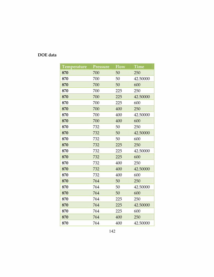
142
DOE data
Temperature Pressure Flow Time
870 700 50 250
870 700 50 42.50000
870 700 50 600
870 700 225 250
870 700 225 42.50000
870 700 225 600
870 700 400 250
870 700 400 42.50000
870 700 400 600
870 732 50 250
870 732 50 42.50000
870 732 50 600
870 732 225 250
870 732 225 42.50000
870 732 225 600
870 732 400 250
870 732 400 42.50000
870 732 400 600
870 764 50 250
870 764 50 42.50000
870 764 50 600
870 764 225 250
870 764 225 42.50000
870 764 225 600
870 764 400 250
870 764 400 42.50000

143
870 764 400 600
885 700 50 250
885 700 50 42.50000
885 700 50 600
885 700 225 250
885 700 225 42.50000
885 700 225 600
885 700 400 250
885 700 400 42.50000
885 700 400 600
885 732 50 250
885 732 50 42.50000
885 732 50 600
885 732 225 250
885 732 225 42.50000
885 732 225 600
885 732 400 250
885 732 400 42.50000
885 732 400 600
885 764 50 250
885 764 50 42.50000
885 764 50 600
885 764 225 250
885 764 225 42.50000
885 764 225 600
885 764 400 250
885 764 400 42.50000
885 764 400 600
900 700 50 250
900 700 50 42.50000
900 700 50 600
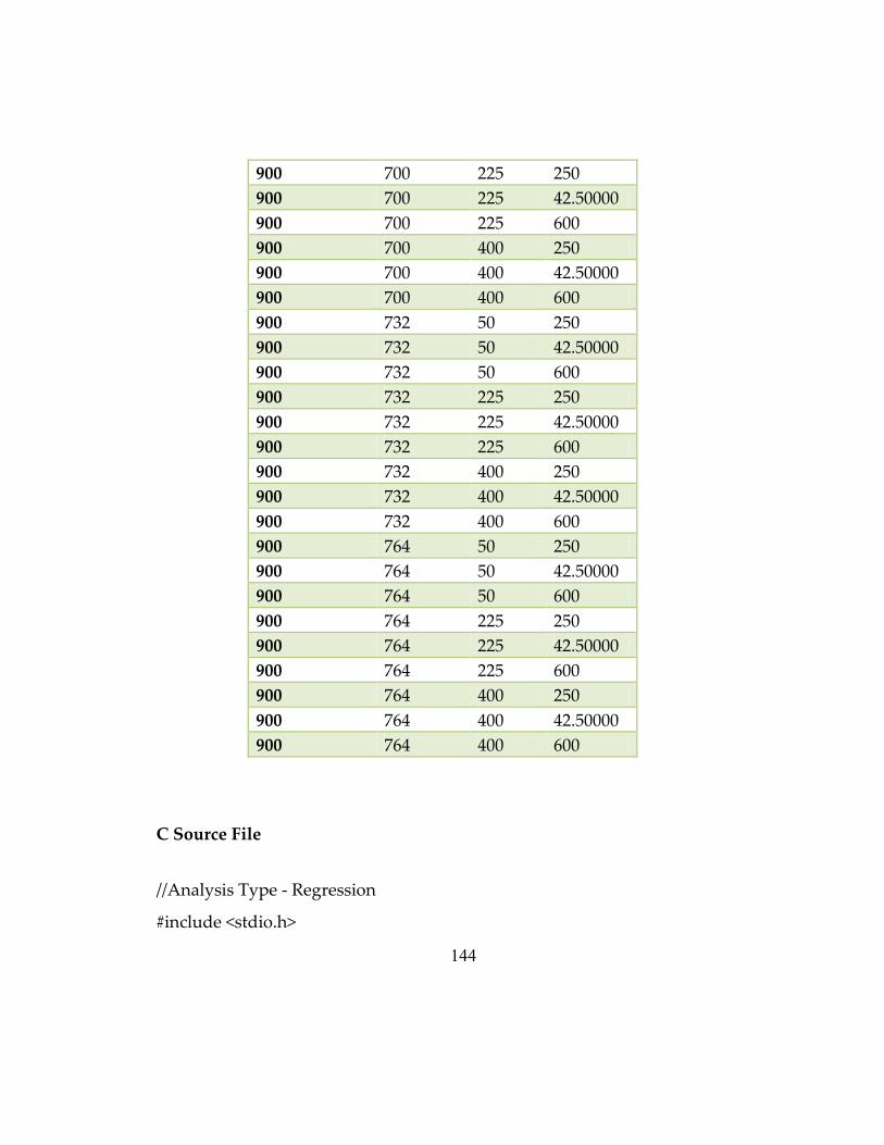
144
900 700 225 250
900 700 225 42.50000
900 700 225 600
900 700 400 250
900 700 400 42.50000
900 700 400 600
900 732 50 250
900 732 50 42.50000
900 732 50 600
900 732 225 250
900 732 225 42.50000
900 732 225 600
900 732 400 250
900 732 400 42.50000
900 732 400 600
900 764 50 250
900 764 50 42.50000
900 764 50 600
900 764 225 250
900 764 225 42.50000
900 764 225 600
900 764 400 250
900 764 400 42.50000
900 764 400 600
C Source File
//Analysis Type - Regression
#include <stdio.h>

145
#include <conio.h>
#include <math.h>
#include <stdlib.h>
double input_hidden_weights[16][4]=
{
{6.88538167880656e+001, 5.19705031137239e+001, 1.96349725020864e-001, -
3.96837035101177e+001 },
{-9.41151995629373e+001, -1.13003504340434e+002, 3.81656846849003e+001,
5.23240862449531e+001 },
{4.01810908021807e+001, -9.18610797701283e+001, -1.04453192467511e+001,
5.36469081765266e+001 },
{-1.56383045945218e+001, -9.06987638452360e+001, -1.01933995373302e+000,
8.40483484092657e+001 },
{5.22265263772885e+001, 8.89616582166964e+001, -3.93660084263335e+001, -
4.43438171715207e+001 },
{1.42040275574771e+001, 1.84972652282273e+001, 3.96386196954803e+000, -
7.87681671339185e+000 },
{3.36355319990229e+001, -1.25864192194514e+002, -4.65829507148270e+001,
6.53305874680016e+001 },
{-7.52932016934223e+001, 5.83281611885973e+001, 3.30854101777050e+000, -
1.31102191213292e+001 },
{1.02433398178607e+001, 1.33528450578865e+002, 9.86575161041711e-001, -
1.26542861376054e+002 },
{-5.45262588816080e+001, -8.60668501080394e+000, -3.21967335331254e+001,
5.00334975291107e+001 },
{-3.36133417636788e+000, -1.27130873750613e+002, -2.28795241300012e+001, -
5.93673720091773e+000 },

146
{-4.94871677241414e+000, 1.75006370691987e+001, 4.70229690719144e+000,
1.61215658839238e+001 },
{-7.82230091690304e+001, -1.54029768119110e+001, -1.27426390300539e+002,
1.61760741125225e+000 },
{3.45486568045511e+001, 6.27126567698776e+001, -9.12086705919135e+001,
4.75735499149714e+000 },
{3.55321485300413e+001, -6.05696311234928e+000, -1.46376742164126e+001, -
3.04507464104846e+001 },
{-3.21699982266888e+001, 1.19627496082985e+002, -7.65554470841906e+001, -
1.42725907753947e+002 }
};
double hidden_bias[16]={ 1.35327813428559e+001, 1.41134751024459e+001,
1.76482123707594e+001, -2.41673416249054e+001, -1.59566330977438e+000, -
1.00669497804693e+001, 3.08661961534460e+001, 6.60304331325891e+001,
8.84922792181880e+000, 1.11914973077307e+001, 7.33639561516985e+000, -
3.20387893627937e+001, 7.09087687782888e+001, 1.49338018849561e+001,
1.45155945812972e+001, 6.17382693600943e+001 };
double hidden_output_wts[1][16]=
{
{-1.83866503181541e+002, -9.08345298647669e+001, 7.35533974495154e+001,
4.73836303200020e+001, 4.87935957704203e+001, -5.98846120080697e+001,
8.34668938379424e+001, -9.83377480284121e+001, 1.23223156059255e+002, -
8.15416774789619e+001, -2.55000470702606e+002, -2.75734810522121e+002,
1.62680971165662e+002, -8.77271503993161e+001, -7.26224338366502e+001,
8.02533927116236e+001 }
};
double output_bias[1]={ -8.78297705012941e+001 };

147
double max_input[4]={ 90000000000e+002, 7.64000000000000e+002,
40000000000e+002, 60000000000e+001 };
double min_input[4]={ 8.70000000000000e+002, 70000000000e+002,
50000000000e+001, 2.50000000000000e+001 };
double max_target[1]={ 1.15000000000000e+003 };
double min_target[1]={ 00000000000e+000 };
double input[4];
double hidden[16];
double output[1];
void ScaleInputs(double* input, double minimum, double maximum, int size)
{
double delta;
long i;
for(i=0; i<size; i++)
{
delta = (maximum-minimum)/(max_input[i]-min_input[i]);
input[i] = minimum - delta*min_input[i]+ delta*input[i];
}
}
void UnscaleTargets(double* output, double minimum, double maximum, int
size)
{
double delta;
long i;
for(i=0; i<size; i++)

148
{
delta = (maximum-minimum)/(max_target[i]-min_target[i]);
output[i] = (output[i] - minimum + delta*min_target[i])/delta;
}
}
double logistic(double x)
{
if(x > 100.0) x = 1.0;
else if (x < -100.0) x = 0.0;
else x = 1.0/(1.0+exp(-x));
return x;
}
void ComputeFeedForwardSignals(double* MAT_INOUT,double*
V_IN,double* V_OUT, double* V_BIAS,int size1,int size2,int layer)
{
int row,col;
for(row=0;row < size2; row++)
{
V_OUT[row]=0.0;
for(col=0;col<size1;col++)V_OUT[row]+=(*(MAT_INOUT+(row*size1)+col)*V_I
N[col]);
V_OUT[row]+=V_BIAS[row];
if(layer==0) V_OUT[row] = tanh(V_OUT[row]);
if(layer==1) V_OUT[row] = logistic(V_OUT[row]);
}

149
}
void RunNeuralNet_Regression ()
{
ComputeFeedForwardSignals((double*)input_hidden_weights,input,hidden,hi
dden_bias,4, 16,0);
ComputeFeedForwardSignals((double*)hidden_output_wts,hidden,output,out
put_bias,16, 1,1);
}
int main()
{
int i=0;
int keyin=1;
while(1)
{
printf("\nEnter values for Continuous inputs\n");
printf("Cont. Input-0(Temp.): ");
scanf("%lg",&input[0]);
printf("Cont. Input-1(P (torr)): ");
scanf("%lg",&input[1]);
printf("Cont. Input-2(gas flow rate): ");
scanf("%lg",&input[2]);
printf("Cont. Input-3(time (min)): ");
scanf("%lg",&input[3]);
ScaleInputs(input,0,1,4);
RunNeuralNet_Regression();
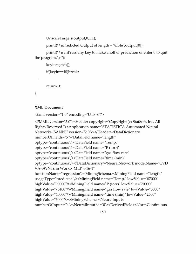
150
UnscaleTargets(output,0,1,1);
printf("\nPredicted Output of length = %.14e",output[0]);
printf("\n\nPress any key to make another prediction or enter 0 to quit
the program.\n");
keyin=getch();
if(keyin==48)break;
}
return 0;
}
XML Document
<?xml version="1.0" encoding="UTF-8"?>
<PMML version="3.0"><Header copyright="Copyright (c) StatSoft, Inc. All
Rights Reserved."><Application name="STATISTICA Automated Neural
Networks (SANN)" version="2.0"/></Header><DataDictionary
numberOfFields="5"><DataField name="length"
optype="continuous"/><DataField name="Temp."
optype="continuous"/><DataField name="P (torr)"
optype="continuous"/><DataField name="gas flow rate"
optype="continuous"/><DataField name="time (min)"
optype="continuous"/></DataDictionary><NeuralNetwork modelName="CVD
VA-SWNTs in Workb_MLP 4-16-1"
functionName="regression"><MiningSchema><MiningField name="length"
usageType="predicted"/><MiningField name="Temp." lowValue="87000"
highValue="90000"/><MiningField name="P (torr)" lowValue="70000"
highValue="76400"/><MiningField name="gas flow rate" lowValue="5000"
highValue="40000"/><MiningField name="time (min)" lowValue="2500"
highValue="6000"/></MiningSchema><NeuralInputs
numberOfInputs="4"><NeuralInput id="0"><DerivedField><NormContinuous

151
field="Temp."><LinearNorm orig="8.70000000000000e+002"
norm="000"/><LinearNorm orig="90000000000e+002"
norm="100"/></NormContinuous></DerivedField></NeuralInput><NeuralInput
id="1"><DerivedField><NormContinuous field="P (torr)"><LinearNorm
orig="70000000000e+002" norm="000"/><LinearNorm
orig="7.64000000000000e+002"
norm="100"/></NormContinuous></DerivedField></NeuralInput><NeuralInput
id="2"><DerivedField><NormContinuous field="gas flow rate"><LinearNorm
orig="50000000000e+001" norm="000"/><LinearNorm orig="40000000000e+002"
norm="100"/></NormContinuous></DerivedField></NeuralInput><NeuralInput
id="3"><DerivedField><NormContinuous field="time (min)"><LinearNorm
orig="2.50000000000000e+001" norm="000"/><LinearNorm
orig="60000000000e+001"
norm="100"/></NormContinuous></DerivedField></NeuralInput></NeuralInpu
ts><NeuralLayer numberOfNeurons="16" activationFunction="tanh"><Neuron
id="4" bias="1.35327813428559e+001"><Con from="0"
weight="6.88538167880656e+001"/><Con from="1"
weight="5.19705031137239e+001"/><Con from="2" weight="1.96349725020864e-
001"/><Con from="3" weight="-3.96837035101177e+001"/></Neuron><Neuron
id="5" bias="1.41134751024459e+001"><Con from="0" weight="-
9.41151995629373e+001"/><Con from="1" weight="-
1.13003504340434e+002"/><Con from="2"
weight="3.81656846849003e+001"/><Con from="3"
weight="5.23240862449531e+001"/></Neuron><Neuron id="6"
bias="1.76482123707594e+001"><Con from="0"
weight="4.01810908021807e+001"/><Con from="1" weight="-
9.18610797701283e+001"/><Con from="2" weight="-
1.04453192467511e+001"/><Con from="3"
weight="5.36469081765266e+001"/></Neuron><Neuron id="7" bias="-
2.41673416249054e+001"><Con from="0" weight="-
1.56383045945218e+001"/><Con from="1" weight="-
9.06987638452360e+001"/><Con from="2" weight="-
1.01933995373302e+000"/><Con from="3"

152
weight="8.40483484092657e+001"/></Neuron><Neuron id="8" bias="-
1.59566330977438e+000"><Con from="0"
weight="5.22265263772885e+001"/><Con from="1"
weight="8.89616582166964e+001"/><Con from="2" weight="-
3.93660084263335e+001"/><Con from="3" weight="-
4.43438171715207e+001"/></Neuron><Neuron id="9" bias="-
1.00669497804693e+001"><Con from="0"
weight="1.42040275574771e+001"/><Con from="1"
weight="1.84972652282273e+001"/><Con from="2"
weight="3.96386196954803e+000"/><Con from="3" weight="-
7.87681671339185e+000"/></Neuron><Neuron id="10"
bias="3.08661961534460e+001"><Con from="0"
weight="3.36355319990229e+001"/><Con from="1" weight="-
1.25864192194514e+002"/><Con from="2" weight="-
4.65829507148270e+001"/><Con from="3"
weight="6.53305874680016e+001"/></Neuron><Neuron id="11"
bias="6.60304331325891e+001"><Con from="0" weight="-
7.52932016934223e+001"/><Con from="1"
weight="5.83281611885973e+001"/><Con from="2"
weight="3.30854101777050e+000"/><Con from="3" weight="-
1.31102191213292e+001"/></Neuron><Neuron id="12"
bias="8.84922792181880e+000"><Con from="0"
weight="1.02433398178607e+001"/><Con from="1"
weight="1.33528450578865e+002"/><Con from="2" weight="9.86575161041711e-
001"/><Con from="3" weight="-1.26542861376054e+002"/></Neuron><Neuron
id="13" bias="1.11914973077307e+001"><Con from="0" weight="-
5.45262588816080e+001"/><Con from="1" weight="-
8.60668501080394e+000"/><Con from="2" weight="-
3.21967335331254e+001"/><Con from="3"
weight="5.00334975291107e+001"/></Neuron><Neuron id="14"
bias="7.33639561516985e+000"><Con from="0" weight="-
3.36133417636788e+000"/><Con from="1" weight="-
1.27130873750613e+002"/><Con from="2" weight="-

153
2.28795241300012e+001"/><Con from="3" weight="-
5.93673720091773e+000"/></Neuron><Neuron id="15" bias="-
3.20387893627937e+001"><Con from="0" weight="-
4.94871677241414e+000"/><Con from="1"
weight="1.75006370691987e+001"/><Con from="2"
weight="4.70229690719144e+000"/><Con from="3"
weight="1.61215658839238e+001"/></Neuron><Neuron id="16"
bias="7.09087687782888e+001"><Con from="0" weight="-
7.82230091690304e+001"/><Con from="1" weight="-
1.54029768119110e+001"/><Con from="2" weight="-
1.27426390300539e+002"/><Con from="3"
weight="1.61760741125225e+000"/></Neuron><Neuron id="17"
bias="1.49338018849561e+001"><Con from="0"
weight="3.45486568045511e+001"/><Con from="1"
weight="6.27126567698776e+001"/><Con from="2" weight="-
9.12086705919135e+001"/><Con from="3"
weight="4.75735499149714e+000"/></Neuron><Neuron id="18"
bias="1.45155945812972e+001"><Con from="0"
weight="3.55321485300413e+001"/><Con from="1" weight="-
6.05696311234928e+000"/><Con from="2" weight="-
1.46376742164126e+001"/><Con from="3" weight="-
3.04507464104846e+001"/></Neuron><Neuron id="19"
bias="6.17382693600943e+001"><Con from="0" weight="-
3.21699982266888e+001"/><Con from="1"
weight="1.19627496082985e+002"/><Con from="2" weight="-
7.65554470841906e+001"/><Con from="3" weight="-
1.42725907753947e+002"/></Neuron></NeuralLayer><NeuralLayer
numberOfNeurons="1" activationFunction="logistic"><Neuron id="20" bias="-
8.78297705012941e+001"><Con from="4" weight="-
1.83866503181541e+002"/><Con from="5" weight="-
9.08345298647669e+001"/><Con from="6"
weight="7.35533974495154e+001"/><Con from="7"
weight="4.73836303200020e+001"/><Con from="8"

154
weight="4.87935957704203e+001"/><Con from="9" weight="-
5.98846120080697e+001"/><Con from="10"
weight="8.34668938379424e+001"/><Con from="11" weight="-
9.83377480284121e+001"/><Con from="12"
weight="1.23223156059255e+002"/><Con from="13" weight="-
8.15416774789619e+001"/><Con from="14" weight="-
2.55000470702606e+002"/><Con from="15" weight="-
2.75734810522121e+002"/><Con from="16"
weight="1.62680971165662e+002"/><Con from="17" weight="-
8.77271503993161e+001"/><Con from="18" weight="-
7.26224338366502e+001"/><Con from="19"
weight="8.02533927116236e+001"/></Neuron></NeuralLayer><NeuralOutputs
numberOfOutputs="1"><NeuralOutput outputNeuron="20"><DerivedField
optype="continuous"><NormContinuous field="length"><LinearNorm
orig="00000000000e+000" norm="00000000000e+000"/><LinearNorm
orig="1.15000000000000e+003"
norm="10000000000e+000"/></NormContinuous></DerivedField></NeuralOutp
ut></NeuralOutputs></NeuralNetwork></PMML>

155
Appendix D
Experimental Data
Temp Flow Time Press Length
880 150 60 700 0
880 150 5 700 325
880 150 60 700 325
880 150 60 700 325
880 150 60 700 325
880 150 60 700 325
880 150 60 700 325
880 150 60 700 325
880 150 30 700 325
880 150 30 700 325
880 150 30 700 325
880 150 30 700 325
880 150 30 700 325
880 150 30 700 325
880 150 60 700 325
880 50 5 700 325
880 20 5 700 325
880 150 60 700 500
880 150 60 700 500
880 150 60 700 500
880 150 60 700 500
880 150 60 700 500
880 150 60 700 500
880 150 60 700 500
880 150 60 700 500

156
880 150 60 700 500
880 150 60 700 500
880 150 5 700 500
880 150 30 700 500
880 150 30 700 500
880 150 30 700 500
880 150 30 700 500
880 150 30 700 500
880 150 30 700 500
880 150 30 700 500
880 150 30 700 500
880 150 30 700 500
880 150 30 700 500
880 150 60 700 650
880 150 90 700 650
880 150 20 700 675
880 150 60 700 1000
DOE data
Flow Time Length
20 50 325
20 32.50000 325
20 600 503.7915
85 50 628.0037
85 32.50000 357.7051
85 600 640.5887
150 50 675
150 32.50000 429.475
150 600 649.8988

157
XML Document
<?xml version="1.0" encoding="UTF-8"?>
-<PMML version="3.0">-<Header copyright="Copyright (c) StatSoft, Inc. All
Rights Reserved."><Application version="2.0" name="STATISTICA Automated
Neural Networks (SANN)"/></Header>-<DataDictionary
numberOfFields="3"><DataField name="Length"
optype="continuous"/><DataField name="Flow"
optype="continuous"/><DataField name="Time"
optype="continuous"/></DataDictionary>-<NeuralNetwork
functionName="regression" modelName="Monte Carlo Data -- Replication 12
(recent) in nonparamet_MLP 2-6-1">-<MiningSchema><MiningField
name="Length" usageType="predicted"/><MiningField name="Flow"
highValue="15000" lowValue="2000"/><MiningField name="Time"
highValue="9000" lowValue="500"/></MiningSchema>-<NeuralInputs
numberOfInputs="2">-<NeuralInput id="0">-<DerivedField>-<NormContinuous
field="Flow"><LinearNorm norm="000"
orig="20000000000e+001"/><LinearNorm norm="100"
orig="1.50000000000000e+002"/></NormContinuous></DerivedField></NeuralIn
put>-<NeuralInput id="1">-<DerivedField>-<NormContinuous
field="Time"><LinearNorm norm="000"
orig="50000000000e+000"/><LinearNorm norm="100"
orig="90000000000e+001"/></NormContinuous></DerivedField></NeuralInput>
</NeuralInputs>-<NeuralLayer activationFunction="logistic"
numberOfNeurons="6">-<Neuron id="2" bias="-2.34605521309488e+000"><Con
weight="-8.43053970865299e-001" from="0"/><Con weight="-
2.31405662902162e+000" from="1"/></Neuron>-<Neuron id="3" bias="-
4.02665223356582e-001"><Con weight="-8.31149712079690e-003"
from="0"/><Con weight="-3.13040212864502e-001" from="1"/></Neuron>-
<Neuron id="4" bias="-2.45349983538043e-002"><Con weight="-

158
1.46958441487193e-001" from="0"/><Con weight="2.21153869088144e+000"
from="1"/></Neuron>-<Neuron id="5" bias="-1.77086489918581e-001"><Con
weight="-4.27712184823327e-001" from="0"/><Con
weight="1.41015887585967e+000" from="1"/></Neuron>-<Neuron id="6"
bias="2.14377123761839e-001"><Con weight="-3.41038575786699e-001"
from="0"/><Con weight="4.11123928698177e+000" from="1"/></Neuron>-
<Neuron id="7" bias="-1.16892250788823e+000"><Con weight="-
3.29827505060424e+000" from="0"/><Con weight="1.50765983953288e+001"
from="1"/></Neuron></NeuralLayer>-<NeuralLayer
activationFunction="identity" numberOfNeurons="1">-<Neuron id="8" bias="-
3.41668192093133e+000"><Con weight="2.63281674121808e+000"
from="2"/><Con weight="2.42953493133018e+000" from="3"/><Con
weight="2.21252553836957e+000" from="4"/><Con weight="1.81199062188609e-
001" from="5"/><Con weight="3.66986350798838e+000" from="6"/><Con
weight="-2.10447746169748e+000" from="7"/></Neuron></NeuralLayer>-
<NeuralOutputs numberOfOutputs="1">-<NeuralOutput outputNeuron="8">-
<DerivedField optype="continuous">-<NormContinuous
field="Length"><LinearNorm norm="00000000000e+000"
orig="00000000000e+000"/><LinearNorm norm="10000000000e+000"
orig="6.75000000000000e+002"/></NormContinuous></DerivedField></NeuralO
utput></NeuralOutputs></NeuralNetwork></PMML>
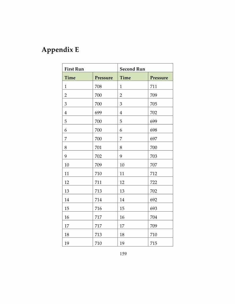
159
Appendix E
First Run Second Run
Time Pressure Time Pressure
1 708 1 711
2 700 2 709
3 700 3 705
4 699 4 702
5 700 5 699
6 700 6 698
7 700 7 697
8 701 8 700
9 702 9 703
10 709 10 707
11 710 11 712
12 711 12 722
13 713 13 702
14 714 14 692
15 716 15 693
16 717 16 704
17 717 17 709
18 713 18 710
19 710 19 715
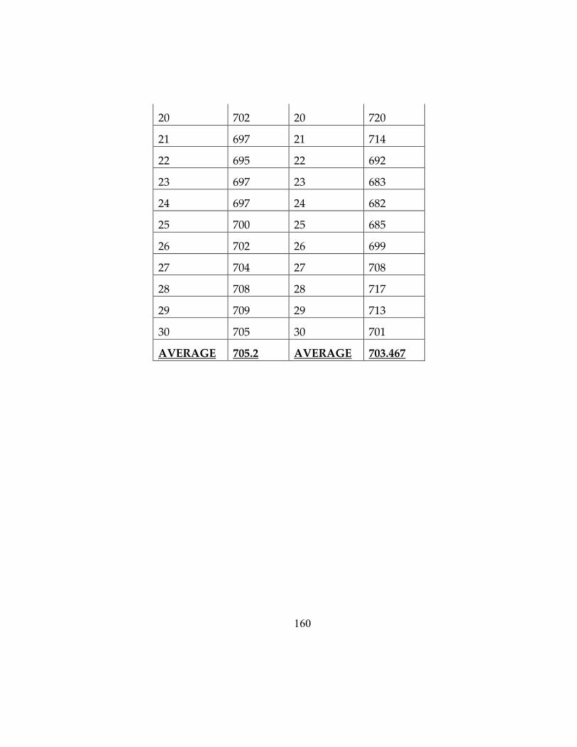
160
20 702 20 720
21 697 21 714
22 695 22 692
23 697 23 683
24 697 24 682
25 700 25 685
26 702 26 699
27 704 27 708
28 708 28 717
29 709 29 713
30 705 30 701
AVERAGE 705.2 AVERAGE 703.467