estimation of the conditional tail index in presence of...
TRANSCRIPT

Outline The problem The estimator Asymptotic properties A simulation study Conclusion and forthcoming studies
Estimation of the conditional tail index in presenceof random covariates
Laurent Gardes (Universite de Strasbourg)Joint work with Gilles STUPFLER (Universite d’Aix-Marseille)
7th International Conference of the ERCIM WG on Computational andMethodological Statistics
1/ 28

Outline The problem The estimator Asymptotic properties A simulation study Conclusion and forthcoming studies
Outline
1. The problem
2. The estimator
3. Asymptotic properties
4. A simulation study
5. Conclusion and forthcoming studies
2/ 28
Outline The problem The estimator Asymptotic properties A simulation study Conclusion and forthcoming studies
The problem
Let (X1,Y1), . . . , (Xn,Yn) be n independent copies of a random pair (X ,Y )such that X takes its values in Rd , d ≥ 1 and that Y given X = x hasconditional survival function
F (y |x) = y−1/γ(x)L(y |x), y > 0,
where L(·|x) is a slowly varying function at infinity.
We address the problem of estimating the function x 7→ γ(x), which iscalled the conditional tail-index of the random pair (X ,Y ).
3/ 28

Outline The problem The estimator Asymptotic properties A simulation study Conclusion and forthcoming studies
Some applications
• the estimation of high risk in finance;
• the description of the upper tail of the claim size distribution forreinsurers;
• study of extreme rainfalls in hydrology.
4/ 28

Outline The problem The estimator Asymptotic properties A simulation study Conclusion and forthcoming studies
Some existing methods
• Fixed design case (the Xi ’s are nonrandom):• Regression model: Smith (1989), Davison and Smith (1990);• Semi-parametric approach: Hall and Tajvidi (2000);• Local polynomials: Davison and Ramesh (2000);• Splines: Chavez-Demoulin and Davison (2005);• Moving window: Gardes and Girard (2008);• Nearest neighbor: Gardes and Girard (2010).
• Random design case:• Maximum likelihood: Wang and Tsai (2009);• Conditional quantile estimators: Daouia et al. (2011, 2013);• Threshold and kernel regression: Goegebeur et al. (2013).
5/ 28
Outline The problem The estimator Asymptotic properties A simulation study Conclusion and forthcoming studies
A first idea
• Let Y1,n ≤ . . . ≤ Yn,n be the ordered statistics.
• The covariate associated with the ordered statistic Yn−i+1,n will bedenoted by X ∗i .
• For k ∈ 1, . . . , n, let Mk(x , h) is the number of covariates amongX ∗1 , . . . ,X
∗k which lie in the ball B(x , h) with center x and radius
h = h(n)→ 0.
6/ 28
Outline The problem The estimator Asymptotic properties A simulation study Conclusion and forthcoming studies
0.0 0.2 0.4 0.6 0.8 1.0
1.0
01
.05
1.1
01
.15
1.2
01
.25
1.3
0
X
Y
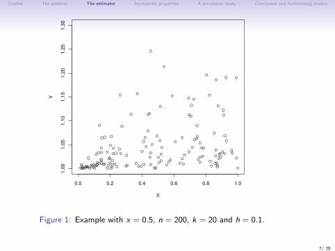
Figure 1: Example with x = 0.5, n = 200, k = 20 and h = 0.1.
7/ 28

Outline The problem The estimator Asymptotic properties A simulation study Conclusion and forthcoming studies
0.0 0.2 0.4 0.6 0.8 1.0
1.0
01
.05
1.1
01
.15
1.2
01
.25
1.3
0
X
Y
Figure 1: Example with x = 0.5, n = 200, k = 20 and h = 0.1.
7/ 28

Outline The problem The estimator Asymptotic properties A simulation study Conclusion and forthcoming studies
0.0 0.2 0.4 0.6 0.8 1.0
1.0
01
.05
1.1
01
.15
1.2
01
.25
1.3
0
X
Y
Figure 1: Example with x = 0.5, n = 200, k = 20 and h = 0.1.
7/ 28

Outline The problem The estimator Asymptotic properties A simulation study Conclusion and forthcoming studies
0.0 0.2 0.4 0.6 0.8 1.0
1.0
01
.05
1.1
01
.15
1.2
01
.25
1.3
0
X
Y
Figure 1: Example with x = 0.5, n = 200, k = 20 and h = 0.1:Mk(x , h) = 5.
7/ 28

Outline The problem The estimator Asymptotic properties A simulation study Conclusion and forthcoming studies
A straightforward adaptation of Hill’s estimator is:
H(x , k, h) =1
Mk(x , h)− 1
k−1∑i=1
logYn−i+1,n
Yn−k+1,n1l‖X∗i −x‖∨‖X∗k −x‖≤h
if Mk(x , h) > 1 and H(x , k , h) = 0 otherwise, where 1l· is the indicator
function and ‖ · ‖ is a norm on Rd .
Problem: the behavior of H(x , k , h) as a function of k is very erratic.
8/ 28
Outline The problem The estimator Asymptotic properties A simulation study Conclusion and forthcoming studies
0.0 0.2 0.4 0.6 0.8 1.0
1.0
01
.05
1.1
01
.15
1.2
01
.25
1.3
0
X
Y
x
0.0 0.2 0.4 0.6 0.8 1.0
1.0
01
.05
1.1
01
.15
1.2
01
.25
1.3
0
X
Y
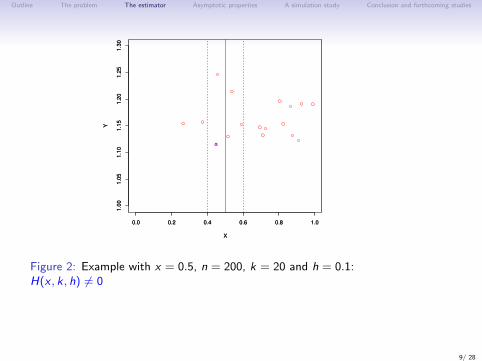
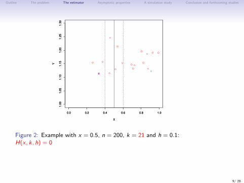
Figure 2: Example with x = 0.5, n = 200, k = 20 and h = 0.1:H(x , k, h) 6= 0
9/ 28
Outline The problem The estimator Asymptotic properties A simulation study Conclusion and forthcoming studies
0.0 0.2 0.4 0.6 0.8 1.0
1.0
01
.05
1.1
01
.15
1.2
01
.25
1.3
0
X
Y
x
0.0 0.2 0.4 0.6 0.8 1.0
1.0
01
.05
1.1
01
.15
1.2
01
.25
1.3
0
X
Y
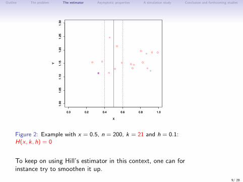
Figure 2: Example with x = 0.5, n = 200, k = 21 and h = 0.1:H(x , k, h) = 0
9/ 28
Outline The problem The estimator Asymptotic properties A simulation study Conclusion and forthcoming studies
0.0 0.2 0.4 0.6 0.8 1.0
1.0
01
.05
1.1
01
.15
1.2
01
.25
1.3
0
X
Y
x
0.0 0.2 0.4 0.6 0.8 1.0
1.0
01
.05
1.1
01
.15
1.2
01
.25
1.3
0
X
Y
Figure 2: Example with x = 0.5, n = 200, k = 21 and h = 0.1:H(x , k, h) = 0
To keep on using Hill’s estimator in this context, one can forinstance try to smoothen it up.
9/ 28

Outline The problem The estimator Asymptotic properties A simulation study Conclusion and forthcoming studies
A smoothed local Hill estimator
We propose to estimate the conditional tail index by an average on j of thestatistics H(x , j , h):
γa(x , kx , h) =1
kx − kx,a + 1
n∑j=2
H(x , j , h)1lkx,a≤Mj (x,h)≤kx
where
• a ∈ [0, 1) is a tuning parameter;
• kx = kx(n)→∞ is a positive sequence belonging to the interval[2/(1− a), n];
• kx,a = b(1− a)kxc where bzc is the integer part of z .
The parameter a controls the number of statistics H(x , j , h) appearing inthe estimator γa.
10/ 28

Outline The problem The estimator Asymptotic properties A simulation study Conclusion and forthcoming studies
Uniform consistency
From now on, it is assumed that X has a probability density function fwhose support is a subset S of Rd (d ≥ 1) having nonempty interior.
We wish to state the uniform consistency of our estimator on a compactsubset Ω of Rd which is contained in the interior of S . We first introducesome regularity assumptions:
(A1) It holds that
• The function γ is positive and continuous on S ;
• The function f is positive and Holder continuous on S ;
• For all x ∈ S , the function F (·|x) is continuous and decreasing.
11/ 28
Outline The problem The estimator Asymptotic properties A simulation study Conclusion and forthcoming studies
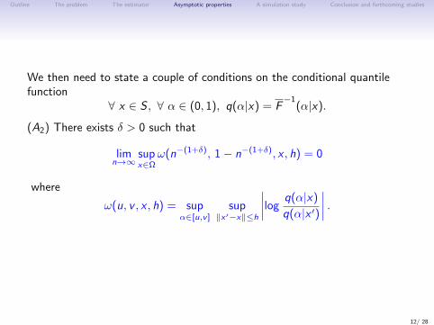
We then need to state a couple of conditions on the conditional quantilefunction
∀ x ∈ S , ∀ α ∈ (0, 1), q(α|x) = F−1
(α|x).
(A2) There exists δ > 0 such that
limn→∞
supx∈Ω
ω(n−(1+δ), 1− n−(1+δ), x , h) = 0
where
ω(u, v , x , h) = supα∈[u,v ]
sup‖x′−x‖≤h
∣∣∣∣logq(α|x)
q(α|x ′)
∣∣∣∣ .
12/ 28

Outline The problem The estimator Asymptotic properties A simulation study Conclusion and forthcoming studies
Finally, note that in our context, it holds that
∀ x ∈ S , ∀ α ∈ (0, 1), q(α|x) = α−γ(x)`(α−1|x)
where `(·|x) is a slowly varying function at infinity.
(A3) For all x ∈ S and t ≥ 1,
`(t|x) = c(x) exp
(∫ t
1
∆(u|x)
udu
),
where c(x) > 0 and ∆(·|x) is an ultimately monotonic function convergingto 0 at infinity.
13/ 28
Outline The problem The estimator Asymptotic properties A simulation study Conclusion and forthcoming studies
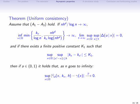
Theorem (Uniform consistency)Assume that (A1 − A3) hold. If nhd/ log n→∞,
infx∈Ω
min
kx
log n,
nhd
kx log(nhd)
→∞, lim
t→∞supx∈Ω
supu≥t|∆(u | x)| = 0,
and if there exists a finite positive constant K1 such that
supx∈Ω
sup‖x′−x‖≤h
|kx − kx′ | ≤ K1,
then if a ∈ (0, 1) it holds that, as n goes to infinity:
supx∈Ω|γa(x , kx , h)− γ(x)| P−→ 0.
14/ 28
Outline The problem The estimator Asymptotic properties A simulation study Conclusion and forthcoming studies
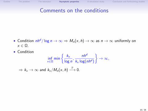
Comments on the conditions
• Condition nhd/ log n→∞ ⇒ Mn(x , h)→∞ as n→∞ uniformly onx ∈ Ω.
• Condition
infx∈Ω
min
kx
log n,
nhd
kx log(nhd)
→∞,
⇒ kx →∞ and kx/Mn(x , h)P−→ 0.
15/ 28
Outline The problem The estimator Asymptotic properties A simulation study Conclusion and forthcoming studies
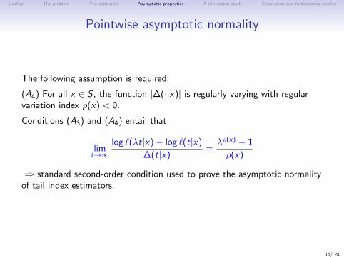
Pointwise asymptotic normality
The following assumption is required:
(A4) For all x ∈ S , the function |∆(·|x)| is regularly varying with regularvariation index ρ(x) < 0.
Conditions (A3) and (A4) entail that
limt→∞
log `(λt|x)− log `(t|x)
∆(t|x)=λρ(x) − 1
ρ(x)
⇒ standard second-order condition used to prove the asymptotic normalityof tail index estimators.
16/ 28

Outline The problem The estimator Asymptotic properties A simulation study Conclusion and forthcoming studies
Theorem (Pointwise asymptotic normality)Assume that (A1), (A3) and (A4) hold. Pick x in the interior of S.Conditionally to the event Mn(x , h) = mx, if
• mx →∞ and kx/mx → 0;
• k1/2x ω(m−1−δ
x , 1−m−1−δx , x , h)→ 0;
• k1/2x ∆(mx/kx |x)→ ξ(x) ∈ R
then for a ∈ [0, 1) one has:
k1/2x (γa(x , kx , h)− γ(x))
d−→ N(ξ(x)AB(a, x)
1− ρ(x), γ2(x)AV(a)
)where if a ∈ (0, 1):
AB(a, x) =1− (1− a)1−ρ(x)
a(1− ρ(x)), AV(a) =
2(a + (1− a) log(1− a))
a2
and if a = 0: AB(0, x) = AV(0) = 1.
17/ 28
Outline The problem The estimator Asymptotic properties A simulation study Conclusion and forthcoming studies
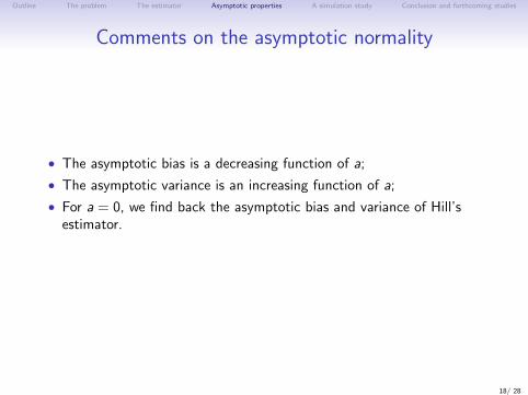
Comments on the asymptotic normality
• The asymptotic bias is a decreasing function of a;
• The asymptotic variance is an increasing function of a;
• For a = 0, we find back the asymptotic bias and variance of Hill’sestimator.
18/ 28
Outline The problem The estimator Asymptotic properties A simulation study Conclusion and forthcoming studies
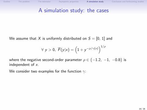
A simulation study: the cases
We assume that X is uniformly distributed on S = [0, 1] and
∀ y > 0, F (y |x) =(
1 + y−ρ/γ(x))1/ρ
where the negative second-order parameter ρ ∈ −1.2, −1, −0.8 isindependent of x .
We consider two examples for the function γ:
19/ 28

Outline The problem The estimator Asymptotic properties A simulation study Conclusion and forthcoming studies
0.0 0.2 0.4 0.6 0.8 1.0
0.2
00
.25
0.3
00
.35
0.4
00
.45
0.5
0
x
γ 1(x
)
0.0 0.2 0.4 0.6 0.8 1.0
0.2
00
.25
0.3
00
.35
0.4
00
.45
0.5
0
x
γ 2(x
)
Figure 3: Functions γ1 (left) and γ2 (right)
Aim: in each case, to estimate the conditional tail-index on a grid of pointsx1, . . . , xM of [0, 1].
20/ 28

Outline The problem The estimator Asymptotic properties A simulation study Conclusion and forthcoming studies
Choice of the parameters
We take a = 3/7: this value of a provides reasonable performances in alarge range of situations.
⇒ it remains to choose:
• the bandwidth h;
• the number of upper order statistics kxi , for 1 ≤ i ≤ M.
Let h1, . . . , hP be a grid of possible values of h. For 1 ≤ i ≤ M,1 ≤ j ≤ P and k ∈ [2/(1− a),Mn(xi , hj)], we set
γi,j(k) = γa(xi , k , hj).
Our selection procedure is carried out in two steps.
21/ 28

Outline The problem The estimator Asymptotic properties A simulation study Conclusion and forthcoming studies
Selection procedure: first step
For every i ∈ 1, . . . ,M and j ∈ 1, . . . ,P, we make a preliminarychoice of kxi for a given hj .
22/ 28
Outline The problem The estimator Asymptotic properties A simulation study Conclusion and forthcoming studies
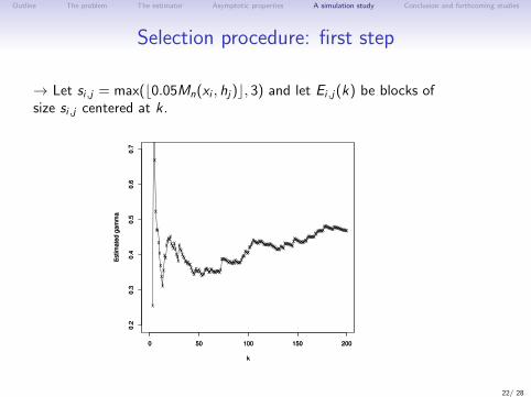
Selection procedure: first step
→ Let si,j = max(b0.05Mn(xi , hj)c, 3) and let Ei,j(k) be blocks ofsize si,j centered at k .
0 50 100 150 200
0.2
0.3
0.4
0.5
0.6
0.7
k
Estim
ate
d g
am
ma
x
x
x
xx
x
x
x
x
x
x
xx
xxxxx
xxxxxxxx
xxxxxxxxxxxx
xxxxxxxxxxxxxx
xxxxxxxxxxxxxxxxx
xxxxxxxxxxxxxxxxxxxx
xxxxxxxx
xxxxxxxxxxxxxxxxxxxxxxxxxxxxxxxx
xxxxxxxxxxxxx
xxxxxxxxxxxxxxxxxxxxxx
xxxxxxxxx
xxxxxxxxxxxxxxxxxxxxxxxx
0 50 100 150 200
0.2
0.3
0.4
0.5
0.6
0.7
k
estim
ate
d g
am
ma
22/ 28
Outline The problem The estimator Asymptotic properties A simulation study Conclusion and forthcoming studies
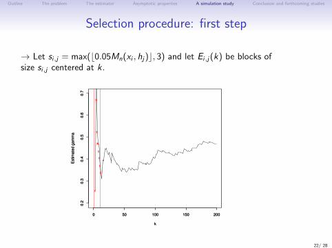
Selection procedure: first step
→ Let si,j = max(b0.05Mn(xi , hj)c, 3) and let Ei,j(k) be blocks ofsize si,j centered at k .
0 50 100 150 200
0.2
0.3
0.4
0.5
0.6
0.7
k
Estim
ate
d g
am
ma
x
x
x
xx
x
x
x
x
0 50 100 150 200
0.2
0.3
0.4
0.5
0.6
0.7
k
Estim
ate
d g
am
ma
22/ 28

Outline The problem The estimator Asymptotic properties A simulation study Conclusion and forthcoming studies
Selection procedure: first step
→ Let si,j = max(b0.05Mn(xi , hj)c, 3) and let Ei,j(k) be blocks ofsize si,j centered at k .
0 50 100 150 200
0.2
0.3
0.4
0.5
0.6
0.7
k
Estim
ate
d g
am
ma
xxxxxxxxxxx
0 50 100 150 200
0.2
0.3
0.4
0.5
0.6
0.7
k
Estim
ate
d g
am
ma
22/ 28
Outline The problem The estimator Asymptotic properties A simulation study Conclusion and forthcoming studies
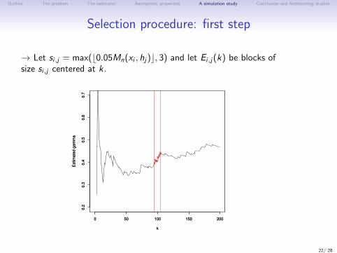
Selection procedure: first step
→ Let si,j = max(b0.05Mn(xi , hj)c, 3) and let Ei,j(k) be blocks ofsize si,j centered at k .
0 50 100 150 200
0.2
0.3
0.4
0.5
0.6
0.7
k
Estim
ate
d g
am
ma
xxxxx
xxxxxx
0 50 100 150 200
0.2
0.3
0.4
0.5
0.6
0.7
k
Estim
ate
d g
am
ma
22/ 28

Outline The problem The estimator Asymptotic properties A simulation study Conclusion and forthcoming studies
Selection procedure: first step
→ Let Ei,j(k∗) be the block where the estimated gammas hasminimal variance.
0 50 100 150 200
0.2
0.3
0.4
0.5
0.6
0.7
k
Estim
ate
d g
am
ma
xxxxxxxxxxx
0 50 100 150 200
0.2
0.3
0.4
0.5
0.6
0.7
k
Estim
ate
d g
am
ma
22/ 28

Outline The problem The estimator Asymptotic properties A simulation study Conclusion and forthcoming studies
Selection procedure: first step
→ In this block, we consider the median of the estimated gammas
0 50 100 150 200
0.2
0.3
0.4
0.5
0.6
0.7
k
Estim
ate
d g
am
ma
x
0 50 100 150 200
0.2
0.3
0.4
0.5
0.6
0.7
k
Estim
ate
d g
am
ma
o
0 50 100 150 200
0.2
0.3
0.4
0.5
0.6
0.7
k
Estim
ate
d g
am
ma
22/ 28
Outline The problem The estimator Asymptotic properties A simulation study Conclusion and forthcoming studies
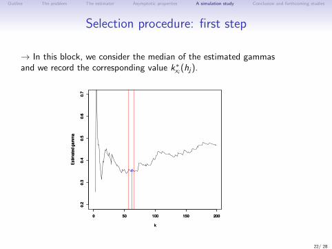
Selection procedure: first step
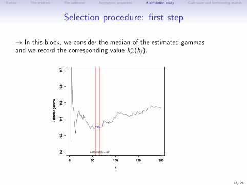
→ In this block, we consider the median of the estimated gammasand we record the corresponding value k∗xi (hj).
0 50 100 150 200
0.2
0.3
0.4
0.5
0.6
0.7
k
Estim
ate
d g
am
ma
o
0 50 100 150 200
0.2
0.3
0.4
0.5
0.6
0.7
k
Estim
ate
d g
am
ma
0 50 100 150 200
0.2
0.3
0.4
0.5
0.6
0.7
k
Estim
ate
d g
am
ma
22/ 28
Outline The problem The estimator Asymptotic properties A simulation study Conclusion and forthcoming studies
Selection procedure: first step
→ In this block, we consider the median of the estimated gammasand we record the corresponding value k∗xi (hj).
0 50 100 150 200
0.2
0.3
0.4
0.5
0.6
0.7
k
Estim
ate
d g
am
ma
0 50 100 150 200
0.2
0.3
0.4
0.5
0.6
0.7
k
Estim
ate
d g
am
ma
o
0 50 100 150 200
0.2
0.3
0.4
0.5
0.6
0.7
k
Estim
ate
d g
am
ma
selected k = 62
22/ 28

Outline The problem The estimator Asymptotic properties A simulation study Conclusion and forthcoming studies
Selection procedure: second step
We now choose the parameter h.
23/ 28

Outline The problem The estimator Asymptotic properties A simulation study Conclusion and forthcoming studies
Selection procedure: second step
→ For every i ∈ 1, . . . ,M, we plot the estimator γi,j(k∗xi (hj)) as afunction of hj , j ∈ 1, . . . ,P
0.05 0.10 0.15 0.20 0.25
0.4
0.5
0.6
0.7
0.8
0.9
h
Estim
ate
d g
am
ma
23/ 28
Outline The problem The estimator Asymptotic properties A simulation study Conclusion and forthcoming studies
Selection procedure: second step
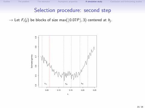
→ Let Fi (j) be blocks of size max(b0.07Pc, 3) centered at hj .
0.05 0.10 0.15 0.20 0.25
0.4
0.5
0.6
0.7
0.8
0.9
h
Estim
ate
d g
am
ma
h10 h50h80
23/ 28

Outline The problem The estimator Asymptotic properties A simulation study Conclusion and forthcoming studies
Selection procedure: second step
→ Compute the standard deviation σi (j) of each block Fi (j) and letσ(j) be the mean of the σi (j), 1 ≤ i ≤ M.
0.05 0.10 0.15 0.20 0.25
0.4
0.5
0.6
0.7
0.8
0.9
h
Estim
ate
d g
am
ma
h10 h50h80
σi(10)
σi(50)
σi(50)
23/ 28
Outline The problem The estimator Asymptotic properties A simulation study Conclusion and forthcoming studies
Selection procedure: second step
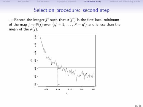
→ Record the integer j∗ such that σ(j∗) is the first local minimumof the map j 7→ σ(j) over q′ + 1, . . . , P − q′ and is less than themean of the σ(j).
0.05 0.10 0.15 0.20 0.25
0.0
00
.01
0.0
20
.03
0.0
40
.05
0.0
6
h
σ(j
)
0.05 0.10 0.15 0.20 0.25
0.0
00
.01
0.0
20
.03
0.0
40
.05
0.0
6
hjx
23/ 28

Outline The problem The estimator Asymptotic properties A simulation study Conclusion and forthcoming studies
Selection procedure: second step
Conclusion We then choose h∗ = hj∗ and k∗xi = k∗xi (hj∗).
23/ 28
Outline The problem The estimator Asymptotic properties A simulation study Conclusion and forthcoming studies
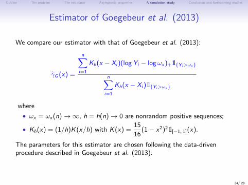
Estimator of Goegebeur et al. (2013)
We compare our estimator with that of Goegebeur et al. (2013):
γG (x) =
n∑i=1
Kh(x − Xi )(log Yi − logωx)+1lYi>ωx
n∑i=1
Kh(x − Xi )1lYi>ωx
where
• ωx = ωx(n)→∞, h = h(n)→ 0 are nonrandom positive sequences;
• Kh(x) = (1/h)K (x/h) with K (x) =15
16(1− x2)21l[−1, 1](x).
The parameters for this estimator are chosen following the data-drivenprocedure described in Goegebeur et al. (2013).
24/ 28

Outline The problem The estimator Asymptotic properties A simulation study Conclusion and forthcoming studies
Methodology
• 100 samples with size n = 1000 of random copies of the pair (X , Y )are generated;
• The estimation is carried out on a grid of M = 35 evenly spaced pointsin [0, 1];
• Selection procedure: P = 100 evenly spaced values of h ranging from0.025 to 0.25 are tested.
MSEs (over the 100 samples) are computed for both estimators.
25/ 28

Outline The problem The estimator Asymptotic properties A simulation study Conclusion and forthcoming studies
SituationEstimator γG Smoothed Hill
of Goegebeur et al. estimator γaγ = γ1
ρ = −0.8 0.0241 0.0115
ρ = −1 0.0157 0.00753
ρ = −1.2 0.00972 0.00512
γ = γ2
ρ = −0.8 0.0321 0.0164
ρ = −1 0.0198 0.0102
ρ = −1.2 0.0148 0.00724
Table 1: MSEs associated to the estimators in all cases.
Both estimations worsen as |ρ| decreases. Remark that the smoothed Hillestimator γa performs better than the estimator γG of Goegebeur et al.(2013) in all the considered situations.
26/ 28

Outline The problem The estimator Asymptotic properties A simulation study Conclusion and forthcoming studies
Conclusion and forthcoming studies
• A new estimator of the conditional tail index was proposed with aprocedure to select the hyper-parameters.
• Its uniform consistency was established.
Future developments include trying to obtain the asymptotic distribution ofthe uniform error
supx∈Ω|γa(x , kx , h)− γ(x)| .
27/ 28

Outline The problem The estimator Asymptotic properties A simulation study Conclusion and forthcoming studies
References
Gardes, L., Stupfler, G. (2014). Estimation of the conditional tail indexusing a smoothed local Hill estimator, Extremes 17(1), 45–75.
Goegebeur, Y., Guillou, A., Schorgen, A. (2014). Nonparametric regressionestimation of conditional tails – the random covariate case, Statistics,48(4), 732–755.
28/ 28