Purdue UniversityPurdue e-Pubs

ECE Technical Reports Electrical and Computer Engineering

4-1-1995

Estimation of Sequential Circuit ActivityConsidering Spatio-Temporal CorrelationsTan Li ChouPurdue University School of Electrical Engineering

Kaushik RoyPurdue University School of Electrical Engineering

Follow this and additional works at: http://docs.lib.purdue.edu/ecetr

This document has been made available through Purdue e-Pubs, a service of the Purdue University Libraries. Please contact epubs@purdue.edu foradditional information.

Chou, Tan Li and Roy, Kaushik, "Estimation of Sequential Circuit Activity Considering Spatio-Temporal Correlations" (1995). ECETechnical Reports. Paper 117.http://docs.lib.purdue.edu/ecetr/117

TR-EE 95-10 APRIL 1995

Elst imat ion of Sequential Circuit Activity Considering Spatio-Temporal Correlations1

Tan-Li Chou and Kaushik Roy Electrical Engineering

Purdue University West Lafayette, IN 47907-1285

Contact person: Kaushik Roy Ph: 317-494-2361 Fax: 317-494-3371

e-mail: kaushik@ecn.purdue.edu

'This research was supported in part by IBM Corporation

Elstirnation of Sequential Circuit Activity Considering Spatio-Temporal Correlations

Abstract

In this paper, we present accurate estimation of signal activity at the internal nodes of sequential logic circuits. The methodology is based on stochastic model of logic signals and takes spatial and temporal correlations of logic signals into con~iderai~ion. Given the State Tranzjition Graph (STG) of a Finite State Machine (FSM), we create an Extended State Transition Graph (ESTG), where the temporal correlations of the input signals are explicitly represented. From the graph we derive the equations to calculiste exact signal probabilities and activities. However, for large circuits the method can be computationally expensive. 'Therefore, we propose an approximate solution method and a Monte Carlo based approach. The approximate method unrolls the next state logic and calculates the activities using a probabilistic technique which considers spatio-temporal correlations of signals. All Monte Carlo based techniques that have been proposed for combinational circuits so far can not be directly applied to sequential circuits. This is because if the initial transient problem is not well dealt with, the estimated activities for some circuit nodes could be off by more thim 100% in comparison to the exact method. The proposed approach deals with this problem by gaining insight from Markov chain theory. Experimental results show that if temporal and spatial correlations are not considered, the power dissipation determined by the approxi mate method can be off by more than 40%. On the other hand, tlie results of the approximate method proposed in this paper are within 5% of that of long run simulation. However, for large sequential circuits and for some applications that require the accuracy of the activitit:~ of individual nodes, experiments show that the Monte Carlo approach is fast and accurate.

1 Introduction

Low power VLSI design has emerged as a major technology driver due to growing markets

in portable computing and communication systems [3, 12, 20, 18, 17, 191. In order to de-

sign circuit's for low power and high reliability, accurate estimation of power dissipation is

required. In CMOS circuits majority of the power dissipation is due to charging and dis-

charging of' load capacitances of logic gates. Such charging and discharging occurs due to

signal transitions. The problem of determining when and how often transitions occur at a

node in a digital circuit is difficult because they depend on the applied input vectors and the

sequence in which they are applied. Therefore probabilistic techniques hatre been resorted

to.

Riesearch directed at estimating signal activity for combinational logic are reported in

(1, 2, 4, 10, 11, 14, 151. In [I], a primary input is specified by two independent parameters:

signal problzbility (probability of being logic ONE) and transition density (,average number

of transitio~ns per second, also called activity). Based on a stochastic model of logic signals,

an algorithm is presented to propagate the activity (which is called transition density in [I])

from primary inputs to the internal and the output nodes. However, the stochastic process

essentially assumes circuits to be asynchronous, that is, the primary inputs can switch at

any time during the clock period. Thus, when applying this approach to real circuits (for

clocked circuits primary inputs normally switch at the leading edges of cloclc only), activity

of a node is always overestimated [2]. Different approaches have been taken to improve

this overestimation. In [8], inertial delay of a logic gate has been considered. Therefore the

glitches that have shorter intervals than the inertial delay have been eliminated when passing

through a low pass filter. In combinational logic synthesis, in order to mi:nimize spurious

transitions due to finite propagation delays, it is crucial to balance all sign'al paths and to

reduce the logic depth [3]. As a result of balancing delays through different p'aths, the inputs

to logic gates may switch at approximately the same time. Hence, Chou et al. in [2] presented

an efficient algorithm to compute the activities at the internal nodes of a circuit considering

signal corre:iations (spatial correlations) and simultaneous switching (temporal correlations).

However, th.e modeling of the correlations between the internal and output nodes is NP hard

[2]. Therefore, trading accuracy with speed is necessary for these techniques.

An alternative approach, a Monte Carlo technique for combinational Logic, has been

proposed in [14, 151. It applies randomly generated input patterns to the sirnulated circuits

and e~timal~es the activity of each node. The activity value is updated ite:ratively until it

converges l,o the true average value with a specified accuracy and a specified confidence

level. However, for nodes that switch infrequently it takes a long time to converge. In

order to get around the slow convergence problem, a threshold value of activity is proposed

in [15]. Falr any node with a activity value less than the threshold value, absolute error

bound is applied rather than percentage error bound. This speeds up the calnvergence while

sacrificing percentage accuracy only on low activity nodes. These nodes usually contribute

little to power dissipation. One of the advantage of this approach is that the desired accuracy

can be specified up-front by the users.

For sequential logic circuits, attempts at estimating activities have been presented in

[4, 10, 111. In [4], the correlation between the applied vector pairs was accurately modeled,

however, the state probabilities were assumed to have uniform distributions. In [lo, 111, the

state probabilities are estimated by using the Chapman-Kolmogorov equations for discrete-

time Markclv chains [21]. However, the input signals were assumed to be teinporally uncor-

related. That is, the input signal at time t is independent of the same input signal at time

t + T, whe~e T is the clock cycle. Therefore, when input signals are temporally correlated,

the activities can be very different from the ones under the assumption given in [lo, 111. Let

us consider the circuit of Figure 1 and its STG (State Transition Graph) in Figure 2. Under

the assumption of having temporally uncorrelated signals, the normalized <activity, a (also

called transition probability) of the input signal equals to 2 * P * (1 - P), where P is the signal

probability. However, if each input signal is temporally correlated, which means that the

inputs can have normalized activities other than 0.5 [2], the probabilities and activities at

the internal nodes can be different. Table 1 shows the different probabilities and activities at

nodes ns l , ns2, and n corresponding to different activities of the input signals. The results

were obtained using logic level simulation. The signal probability of the input I is assumed

to be 0.5. If the primary input is temporally uncorrelated, its normalized activity equals to

2 x 0.5 * (1 - 0.5) = 0.5.

In this paper, we assume that the input signal distributions are represented by probabil-

ities and activities of the input signals. Therefore given a state transition graph (STG) of a

finite state inachine (FSM), we can create an extended state transition graph (ESTG). Each

state in ESrC'G is represented by a present state in STG and the next primary input vector

(corresponding to next state). The temporal correlation of the input signals are explicitly

represented by ESTG. In [lo, 111, since the temporal correlation is neglected., the transition

probability of STG (the probability of transition from one state to another state) is com-

Table 1: Probabilities and normalized activities corresponding to different activities of input signals

Figure 1: An example sequential circuit.

Figure 2: A general model for sequential logic circuit.

pletely determined by the present input vector. We present an exact method to estimate

signal activity which is similar to [lo, 111. However, we apply the Chapman-Kolmogorov

equations to the ESTG rather than STG. The exact method requires the solution of a linear

system of c:quations of size at least 2M and at most 2M+N, where M is the number of the

latches (flip-flops) and N is the number of the primary inputs. For large circuits, the method

may be conlputation-time intensive. Hence, we also present two different approaches: an ap-

proximate tlolution method and a Monte Carlo based technique to estimate the probabilities

and activities at the internal nodes of a circuit.

The aplproximate solution method first unrolls the the circuit k times with assigned

initial values at the state bits. The signal probabilities and activities of the state inputs

are then ca,lculated by applying a method similar to the one proposed by us in [2]. Since

the approximate method does not assume the knowledge of STG, it is applicable to general

sequential circuits. However, this method, like the one for combinational circuits [2], must

trade off accuracy for speed. Such a trade-off results in loss of accuracy of individual node

activities. On the other hand, Monte Carlo seems to be a good solution for sequential circuits.

However, all Monte Carlo based techniques (statistical techniques) that have been proposed

for combinational circuits do not apply directly to sequential circuits [9]. A similar problem

that causes the stopping criteria erroneously to terminate the simulation for combinational

circuits [14] exists for sequential circuits, too. Furthermore, the heuristic method to deal

with the problem in combinational circuits proposed by [14] cannot be applied to that in

sequential circuits. Like all the steady-state parameters in simulation, the sc~mple mean has

the initial t,ransient problem, or the startup problem [22]. In order to reduce the bias of

the sample mean, ESTG is thought of as a Markov chain [21] network. Given the following

parameters: an upper bound of the second largest eigenvalue, the probability of a near-closed

set, and an upper bound on the relative error of the probability of the near-closed set, we

can determine the length of warmup period required to reduce the bias. After the warmup

period, the sampling begins and sample mean is calculated and the statistical estimation

method proposed in [15] can be applied to the analysis of the output data.

The rest of the paper is organized as follows. Section 2 reviews signal probability and

activity definitions. The basic definitions concerning STG and FSM are also given in the

same section. Section 3 describes an exact method of calculating the signal probabilities and

activities for sequential circuits, considering temporal correlation of input signals. Section 4

presents an approximate but computationally efficient method of estimating signal activity

Combinational Logic Primary outputs

Figure 3: A General Synchronous Sequential Logic Circuit.

P

in sequential circuits. Section 5 introduces a Monte Carlo approach and discusses the initial

transient piroblem with sequential circuits. Section 6 gives a more complete but brief intro-

duction to Markov chain theory. Based on Markov chain theory, a method ito deal with the

initial transient problem is proposed. The reduction of sample variation is also addressed

there. Expttrimental results are presented in section 7. The conclusion is given in Section 8.

-

2 Preliminaries and Definitions

Present state inputs - Next state inputs

In this section we describe the representation of sequential circuits and ST(;, followed by a

brief discussion on signal probability, activity, and power dissipation in CMOS.

Representation of Sequential Logic Circuits: A general model for a synchronous se-

quential circuit (Mealy machine) is shown in Figure 3. We denote the input vector to the

combinatioilal logic as U. U-T, Uo, and UT represent U at time -T, 0, and T respectively,

where T is the system clock cycle. Input vector U consists of two parts: primary inputs I

and state irlputs S. Accordingly, < I-T, BS >, < Io, PS > and < IT, NS ;> correspond to

U-T, Uo ant1 UT. Here I-T, lo, and IT are primary inputs at time -T, 0, and F . Particularly,

we denote state inputs at -T, 0, and T as previous state BS, present state PS, and next

state NS rt:spectively. PS is completely determined by < I-T, BS > or U-T, and NS by

< I,, PS > or Uo.

STG is represented by a directed graph G(V, E), where each vertex Si E V represents a

state of the FSM and each edge e;,j E E represents a transition from S, to S, . Each state S,

also corresponds to an instance of the vector S (state inputs). F(Si, I) = Sj alenotes that the

machine makes a transition from state Si to Sj due to the primary input vector I. We call

F(-) the next state function. Therefore, we have F(PS, Io) = NS and F(BS, I-T) = PS.

We assume that the implemented sequential circuit or the STG do not contain periodic-

states.

Signal Probabil i ty a n d Activity:

This section briefly describes the model used in [I, 21 for estimation of signal activity. The

primary inputs to a sequential circuit are modeled as mutually independent Strict-Sense

Stationary (SSS) mean-ergodic 0-1 processes. Under this assumption, the p:robability of the

primary input logic signals x i ( t ) , i = 1 . . . n, assuming the logic value ONE at any given time

t becomes a constant, independent of time, and is called the equilibrium probability of the

random signal x i ( t ) . This is denoted by P ( x ; ) . The activity A(x ; ) at a prirnary input x; of n ~ . (7') the module is defined as limT,, n"T(T) and equals the expected value of *-. The variable

nZi is the number of switching of x i ( t ) in the time interval ( - T / 2 , T / 2 ] . Since sequential

digital circuits or the corresponding STG contain no periodic-states, it can be shown that

the signals at the internal and output nodes of the circuit are also SSS and mean-ergodic.

Further, the Boolean functions describing the outputs of a logic module are decoupled from

the delays inside the module by assuming the signals to have passed through a special delay

module prior to entering the module under consideration. Therefore, the task of propagating

equilibrium probabilities through the module is transformed into that of propagating signal

probabilities.

Assume all primary inputs to the module switch only at the leading edge of the clock

and the mcldule is delay-free. Every signal x at the internal or output node of the circuit

become a discrete-time stochastic process. Therefore, x ( t ) represents the 1og;ic value for the

time intervitl ( t , t + TI, where t is some leading edge of the clock cycle ancl T is the clock

cycle of the circuit module. This is due to the fact that during the interval. the signal y ( t )

does not change value. We denote P ( y ( t ) ) as the probability of node y being logic ONE in

the time in1,erval ( t , t + TI. Similarly, P ( y ( t ) ) is the probability of node y being logic ZERO

in the time interval ( t , t +TI. If one selects a clock cycle at random, the proba~bility of having

a switching at time t at node y is A ( y ) / f . A ( y ) is the activity at node y an'd f is the clock

frequency [1.3]. We define the normalized activity a ( y ) as A( y )/ f . In [lo, 1 : I . ] , a (y ) is denoted

as transitioii probability. Therefore,

Since y is SSS, P ( y ( t ) ) = P ( y ( t + T ) ) . Furthermore, we have

Hence, P(y(t - T)ij(t)) = P(y(t - T)y(t)) = ta(y). Similarly, we can show the following [2],

and

where P(.l-) represents the conditional probability.

Power Dissipation in CMOS Logic Circuits

Of the three sources of power dissipation in digital CMOS circuits - switching, direct-path

short circuit current, and leakage current - the first one is by far the dominant. Ignoring

power dissipation due to direct-path short circuit current and leakage current, the average

power dissipation in a CMOS logic is given by POWER,,,, = +Vd2d xi CiA(i), where Vdd is

the supply voltage, A(i) is the activity at node i, and Ci is the capacitive load at that node.

The summ;~tion is taken over all nodes of the logic circuit. It should be observed that A(;)

is proportional to a(i). C; is approximately proportional to the fanout at that node. As

a result, the normalized power dissipation measure defined as = xi f~znout; x a(i) is

proportional to the average power dissipation in CMOS circuits. The parameter, fanout; is

the number of fanouts at node i.

3 Siginal Activity Considering Temporal Correlation of the Input Signals

In this section, we will derive an accurate method of calculating signal activity. Some basic

assumptions of our exact method will be introduced. Based on some of the assumptions,

we will extend STG to ESTG (extended STG) and derive state probabilities by applying

Chapman-h:olmogorov equations to the ESTG. Therefore, by explicit or implicit state enu-

meration, we can calculate the exact probabilities and activities of internal nodes and state

inputs.

3.1 Assumptions for the Exact Method

As mentioned in section 1, we assume that the glitches can be neglected if all the paths

are balanced and the logic depth is reduced. Delays are decoupled from the circuits and

are assumed to be neglected. Also, we assume that primary inputs to a sequential circuit

are modeled as mutually independent (SSS) mean-ergodic 0-1 process. Eaclh primary input

is associated with a signal probability and an activity. For combinationa,l circuits, these

assumptions will completely determine all the internal and the output nodes of the circuits.

However, more information is necessary for sequential circuits. NS of the sequential cir-

cuits depends on < lo, PS >, PS on < I-T, BS >, and hence N S on < I-T, lo, BS >. Moreover, we can extend this procedure and reach the conclusion that IYS depends on

< lo, I-T, i r - * ~ , . . . >, that is, the whole history of the primary inputs. This makes the

calculation complicated and computationally forbidden. Therefore, we assurne that for each

primary input x i , x i ( t ) only depends on x;(t - T ) . That is, if its present x,(t - T ) is spec-

ified, its past xi(t - 2T)) x;(t - 3T), . . . have no influence on the future x(t:l. This is called

discrete-time Markov chain [21] with 2 states, ZERO and ONE. Therefore, if x;(t - T ) is

known, frorn equation 2 the probability of x; ( t ) is determined by its signal probability and

activity as ~Eollows:

P ( x i ) - x a(x i ) x a(xi) P ( ~ ~ ( t ) I x , ( t - T ) ) = , P ( i i , ( t ) l ~ ; ( t - T ) ) = --) 2

P(xi) Pl[xi) 1 - 2 x a (x i ) 1 - P ( x i ) - x a (x i )

P(x;(;t)Jii;(t - T ) ) = P(ii;( t) lz;( t - T ) ) = 1 - P(x; ) ) 1 - P ( x ; ) (3 )

As a result of the assumption of Markov chain inputs, the following equations hold:

P(x;(t) lx;(t - T ) . . . x;(t - TIT)) = P(x; ( t ) (x i ( t - T ) )

P ( ~ ; ( i ! ) ~ i ( t - T ) . . . x;(t - nT)lxi(t - T ) . . . x;(t - n T ) ) = P(x;(t) lx;(t .- T ) ) . (4)

The assumption that the primary input signal is a discrete-time Markov chain implies the

constructioil of ESTG built from the STG of the FSM. We will explain it in the following

sect ion.

3.2 Sta.te Probability Calculation from ESTG

Given the STG of a sequential circuit or an FSM, we can build ESTG and calculate the

probability of a state of the ESTG. Consider the STG of Figure 2. Let P ( S , ) denote the

state probal~ility, that is, the probability of the machine being in state S;. P(e ig j ) represents

the transition probability, which is the probability of the machine making a transition from

state S; to Sj. However, P(e;j) depends not only on present primary inputs but also on the

previous inlmts, and hence it depends on S;. As a result, P(e i j ) is not equal to the probability

of the present primary input vector I that satisfies F(Si, I ) = Sj, where F( . ) denotes the

next state junction mentioned in section 2. That is, P ( N S ( P S ) # P(Io), where P ( N S ( P S )

denotes the transition probability from PS to N S and F(PS, 10) = NS. Since P(ei$) in

not known, we can not apply Chapman-Kolmogorov equations to STG. This motivates us

to create E I ~ T G from STG.

ESTG i:s represented by a directed graph G(V1, El), where each vertex Si E V' represents

a state of the FSM and each edge e:,j E E' represents a transition from S;' to Si. Each state

S;' also corresponds to an instance of the vector < S, I > (state inputs and primary inputs).

Therefore, ~f the sequential circuit under consideration has N primary independent inputs

and M state inputs, the number of the states of the ESTG can be 2 N + M . That is, a state S

in STG is split into 2N states in ESTG. In this way, each state in ESTG keeps track of the

value of the present primary input vector.

For example, Consider the STG of Figure 2. The corresponding EST" is shown in

Figure 4. In Figure 4, each state is represented by two present state bits and one present

input, that is, psl,ps2, Io. The variable attached to each edge in Figure 4 is the next input

(input at time T). The state Sl in the STG of Figure 2 is split into Slo and Sll in ESTG.

By definition the machine will make a transition from state < BS, A'-T > to state

< PS, I. > if the present primary input vector is Io, and from < PS, lo > to < NS, IT > if the next primary input vector is IT. Therefore, the transition probability from < PS, I0 > to < N S , I r >, denoted as P(< NS, IT > 1 < PS, lo >), equals to P(I:rl < PS, l o >)

if F1(< PS', I. >,IT) = < NS, IT >, where F1(S;', IT) = S: denotes t h , ~ t the machine

makes a trimsition from state S;' to Si due to the next primary input vector. Further-

more, since the primary inputs are assumed to be Markov chain, IT depends on I. only,

P(ITI < PS', lo >) = P(ITIIo). We have:

P(< IVS, IT > ) < PS, 10 >) = P( IT JIo), if F1(< PS, I 0 >, IT) =*< NS, IT >,

= 0, if F1(< PS, I, >, IT) #< NS, IT > . (5)

where P(IT 1 Io) is the conditional probability.

For instance, let us assume that the FSM is in STG state Sl (Figure 2) with primary

input value of 1. The next STG state will be S2. However, in the ESTG (Figure 4) the state

transition is different. At first, the FSM is in ESTG state Sll since the primary input value

is 1 (if the primary input value is 0, it is in Slo instead), Up to this point, we know that the

next ESTGl is either S20 or S21, which correspond to a STG state S2. Bulb the exact next

ESTG state depends on the next primary input value. If the next primary input value is 1

(O), the next ESTG state is S21 (S20). Because the present input value is 1 and the next

input value is 1 (O), the transition probability from Sll to S21 (S2,) is P(13plIo) (P( ITl~o) ) .

Since wle assume that the primary inputs are mutually independent, we have N

IT 110) = n P(xi(T) Ixi(O)), i=l

(6)

where x; is one of the N primary inputs. Equation 6 can be calculated using equation 2.

For the ESTG, we can obtain its state probabilities by solving the Chapm.an-Kolmogorov

equation [21] as follows:

P(S,') = C P(I ; l I j )P(s ; ) i= l ,2 , . . . L - 1 jEINSTATE(I)

L 1 = C P(s;)

j=1 (7)

where P(S;':) = P(< Si, I; >) and I N S T A T E ( i ) is the set of fanin states of :?: in the ESTG.

Let us assume that the ESTG have L states. For STG, we can obtain its stake probabilities

by summing all the ESTG states that correspond to the same state in STG. That is,

3.3 Signal Probability and Activity

We first consider the signal probabilities and activities of the internal nodes and the primary

outputs. Let y denote an internal node or a primary output. Node y can be represented by

a logic function f (< S, I >) with state inputs S and primary inputs I . Let y(0) and y(T)

denote f (< PS, lo >) and f (< NS, IT >) respectively. Since y is SSS aind N S = F ( <

PS, I. >), vre have

and

4 ~ ) = P(y(0) @ Y(T)) = p ( f (< PS, I o >) @ f (< NS, IT >))

= p(f(< P S , I o > ) @ f ( < F(< PS , Io>) , IT >)).

v Figure 4: Extended state transition graph.

By summing up all the terms over all possible ESTG states, that is, by the total probability

theorem [21], we have

P(Y) = C < P S , Z o >€(all ESTG states)

f (< PS, I0 >)P(< PS, I0 >),

a(?/ ) = C <PS,.ro>€(all ESTG states)

P(f(< PS, l o >) $ f (< F(< PS, I o >),IT >)I < PS, lo >)

x P(< PS, .Io >).

Notice that given a state < PS, I. > in ESTG,

P(f (<: PS, l o >) $ f (< F(< PS, I o >), IT)\ < PS, I o >)

is a function of IT only.

Given the state encoding, each STG state is represented by state inputs $0, s l , . . . , S M - ~ ,

where M is the number of flip-flops. Similarly, each ESTG state is represented by state

inputs so,sll, . . . , s ~ - 1 and primary input vector Io. Therefore, for the node of the state

input s;, we can calculate its probability by summing up all the probabilities of ESTG states

whose s; value is 1 in its representation. That is,

where S E M ( i ) is the set of states whose encodings have the ith bit equal l;o ONE. In the

same way, hy summing all the probabilities of ESTG states whose s; value is v at present

The probabilitiw and activities of stale inputs feedback in Phase I1

JJI-[L,

Figure 5: Unrolling of the sequential circuits k times.

athatage

time 0 and is @ at next time T, we have

C P(< PS, I0 >). PS~S_EN(~)NSES-EN(i)

L

4 An Approximate Solution Method

PS - fl

As mentioned before, the exact method may require solving for a linear system of equations

of size 2IV+", where N is the number of primary inputs and M the number of flip-flops. For

large circuil,~ with large number of primary inputs and flip-flops, the exact method is compu-

tationally expensive. Therefore, we propose an approximate method which takes temporal

correlations of primary inputs into account. We unroll the sequential circuit b'y k time frames

I - ... 4-1

N s l k 1)

as shown in Figure 5. As k approaches infinity, the unrolled circuit is the co~iceptually same

Or- 1 Fth - ) shge NS 0

as the unrolled sequential circuit. However, it is computationally expensive to unroll the

circuit infinite times. As a result, we unroll it k times and approximately capture the spatial

and temporal correlations. At first, we need the signal probabilities and activities of the

present state bits of the oth stage (PSo) to calculate the signal probabilities a~nd activities at

1st slage

the internal nodes and outputs. In sequential circuits, the signal probabilities and activities

at PSo are tihe same as those at the next state bits of the (k - l)th stage (Nd!i'k-l) if glitches

are neglected. Though this is not true for the k-unrolled circuits, it implies el method to get

initial values for PSo. Therefore, we can obtain the approximate signal pi-obabilities and

activities at the PSo by assigning initial values to PSo, calculating the signal probabilities

and activities at NSk-l, and assinging the values of NSk-l to PSo. Once we have the more

accurate initial values, we can compute the signal probabilities and activities at all nodes at

the (k - l)'h stage. We will explain the details of the solution method by dividing it into

two phases.

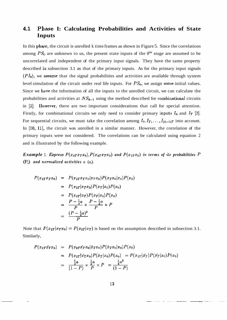
4.1 Phase I: Calculating Probabilities and Activities of State Inputs

In this phase, the circuit is unrolled k time frames as shown in Figure 5. Since the correlations

among PScI are unknown to us, the present state inputs of the Oth stage are assumed to be

uncorrelated and independent of the primary input signals. They have the same property

described in subsection 3.1 as that of the primary inputs. As for the primary input signals

(PIo), we assume that the signal probabilities and activities are available through system

level simulation of the circuit under real life inputs. For PSo, we assign some initial values.

Since we have the information of all the inputs to the unrolled circuit, we can calculate the

probabilities and activities at NSk-l using the method described for combillational circuits

in [Z]. Hawever, there are two important considerations that call for special attention.

Firstly, for combinational circuits we only need to consider primary inputs I 0 and IT [2].

For sequential circuits, we must take the correlation among l o , IT , . . . , I ( k - 1 ) ~ into account.

In [lo, 111, the circuit was unrolled in a similar manner. However, the correlation of the

primary inputs were not considered. The correlations can be calculated using equation 2

and is illustrated by the following example.

Example I. Express P ( x ~ ~ x ~ x ~ ) , P ( x ~ ~ ~ ~ x ~ ) and P(xzTxo) in t e rms of i ts probabilities P

(P,) and normalized activit ies a (a,).

Note that = P(xzT(xT) is based on the assumption described in subsection 3.1.

Similarly,

0-th stage 1st stage

Figure 6: An example of a temporally reconvergent node in the unrolled circuit of Figure 1 .

Therefore, we have

Secondly, reconvergent nodes of sequential nodes are different from those of the combi-

national ones [2]. Consider the circuit of Figure 6, which is a 2-unrolled circuit of Figure 1 .

Only from .topological analysis, it seems that IT and ns2O are independent of each other.

That is, there does not exist a common ancestor of node IT and node ns2O. An ancestor y

of a node z is defined as a node such that there is a directed path from y to z. However,

ns2' is topologically dependent on node 1°, and the primary inputs 1° and IT are tempo-

rally correlated. As a result, IT and ns2' are not independent. Here node I is defined as

a temporally reconvergent node as opposed to a topologically reconvergent node. Following

the calculation of the probabilities and the activities of next state inputs of the (k - l ) t h

stage, we cam calculate the total power dissipation of the circuit in Phase 11.

4.2 P base 11: Calculating Probabilities and Activities of Internal Nodes

In this phase, the probabilities and the activities of the state inputs of the ( I t h stage are set

equal to those of the next state inputs of the ( k - l ) t h stage. Under the sarne assumptions

as those of Phase I, we can by the same method, calculate all the probabilities and the

activities of the internal nodes, including the primary outputs and the next state inputs of

the ( k - I)~,'' stage.

Before we leave this section, it is worth mentioning that the approxima,te method is in

fact exact lor pipelined circuits. This is due to the fact that pipelined circuits do not have

feedback (present state inputs).

5 Monte Carlo Based Techniques and Their Problems When Applied to Sequential Circuits

In the approximate method the more we unroll the circuit, the more accurate results we may

get (theoretically). However, unfortunately we need to handle more primary inputs. If the

circuit is u~lrolled k time frames, the number of primary inputs are N * k + IEM, where N and

M are the :number of primary inputs to the sequential circuits and the number of state bits

respectiveljr. This implies that we must partition the unrolled circuits to trade accuracy for

speed. Hence, in practice, more stages of the unrolled circuit do not necessaxily imply more

accurate reisults if the unrolled circuit is partitioned for lower CPU time. In this section, we

review the Monte Carlo based technique proposed in [15] for combinational ci1:cuits. However,

this technique can not be directly applied to sequential circuits without any modification.

We will examine the initial transient problem inherent to sequential circuits while applying

Monte Car1.0 based technique to them.

5.1 A :Monte Carlo Approach for Combinational circuits

The basic .idea of Monte Carlo methods for estimating activity of indiviclual nodes is to

simulate a circuit by applying inputs of random patterns. The convergence of simulation

can be obtained when the activities of individual nodes satisfy some stopping criteria.

We can use random number generators to generate input patterns conforming to given

activities and probabilities. During a given period, say T (T clock cycles), we count the

number of transitions at each node, nl and call the value n l /T a random sample. T is called

the sample length in this paper. The process is repeated I ' times to have I' independent

samples, a, = nj/T, j = 1 - . . K, by using different seeds for the random nurnber generators.

The sample mean is defined as a = (Cy=, aj)/I'. For large I<, a will approa,ch the expected

value of a, .which is limT,, nT/T, and is denoted as n since the signal at each node is mean-

ergodic (section 2). n~ is the number of transitions in the time interval (3, $]. Similarly,

for large K' the sample standard deviation s will approach the true standard deviation o.

Furthermore, according to the Central Limit Theorem [21] ct is a random variable with mean

a and has a distribution approaching the normal distribution if K is large (typically 2 30).

Likewise o e s a . It has been shown in [14, 151 that for (1 - a ) x 100% confidence the

following inequality holds:

where za12 is a specific value such that the area under the standard normal distribution from

za/2 to oo is a/2. Therefore, if

la - 2,129 la - iil €1 we halve - 5 - 5 el , and hence - 5 - = c,

a f l a a 1 - €1

Equation 1'2 is the stopping criterion for (1 - a) x 100% confidence and e is an upper bound

on the rela1:ive error.

If any node in the circuit has a very low activity, that is, its ii << 1, by equation 12 the

number of samples required can be very large. This results in slow convergence. However,

since these low-activity nodes contribute little to power dissipation, a modified stopping

criterion is proposed in [15]. One can specify a particular threshold value a,,;,, below which

the activities of nodes are less important. Hence one may not wait for those nodes to converge

to a value within a certain percentage of error. Furthermore, if

Ja - z a / 2 ~ aminel we hi~ve - <-<-, - a f l

and hence Ja - nl <_ a,,in€l. a a

Therefore, equation 13 becomes the stopping criterion (with 6, < amin) for (1 - a ) x 100%

confidence and aminel is an absolute error bound (not a percentage error bound).

5.2 Pr'oblem of Initial Transient

Like all the steady-state parameters in stochastic processes, samples can be severely biased

if proper care is not taken. The Monte Carlo approach falls into the category of replication

approach. Therefore, it is natural to consider the replication/deletion approach to reduce

the bias caused by initial states [22]. In each sample, we start with a warmup period, say P

cycles, without counting any transitions. After the warmup period, we count the transitions

as before for a period of sample length. The problems of how to choose an initial state for

each sample and of how long the warmup period should be will be discussed in section 6.

Figure 7: Examplel: A STG of a sequentia.1 logic circuit.

Table 2: Results on the STG of Examplel

Let us consider the STG of Figure 7. The primary inputs x; ( i = 1 . . .7) are assumed to

be independent of each other. We can derive the next state bits nso and nsl as follows,

The output, y , equals to sox7. Assume all the signal probabilities (P(x;)) and normalized

activities ((z(xi)) of the primary inputs are 0.5 and 0.5 respectively. That is, we can apply

Chapman-lColmogorov equations to STG since the primary inputs are teinporally uncor-

related andl have their normalized activities being 2 * 0.5 * (1 - 0.5) or O.!j. Monte Carlo

methods with different choices of initial states and with or without warmiup periods have

been tried. The results are summarized in Table 2. In the table, n(y), a.(sl), and a(s0)

are the no~nmalized activities of output y and of state bits, s l and SO respectively. Exact

represents the results of the exact method introduced in Section 3. S; ICIrC is the Monte

Carlo method with initial state S;, where So, S1, S2 and S3 are represented by < l a , ;lsO,

s l d , and .slsO respectively. MC denotes the Monte Carlo method with a random initial

state (uniformly distributed) for each sample. Wl MC and W2 MC are Monte Carlo based

methods with a random initial state and warmup periods of 109 cycles ( Wl MC) and of

1148 cycles (W2 MC) respectively (the significance of these numbers, 109 and 1148, will

be clear from section 6). S; MC, MC and Wl MC all have the same sample length of 100

cycles while W2 MC's sample length is of 3000 cycles. The Monte Carlo rnethods tried in

the table are based on 5% error, 95% confidence, and a,i, = 0.3. Observe that the transition

probabilities (the probability of making a transition) from state ;lsO to state sls0 and vice

versa are 0.0156 and 0.125. They are so low that it is very unlikely that a transition will

occur between {So, S2} and {S1, S3}. Since the initial states of S1 MC and S3 MC are S1

and S3 respectively, without warmup periods the samples of S1 MC and S3 ~MCare collected

from among states S1 and S3. This is also true for the samples of So MC anti S2 MC. Unfor-

tunately, the sample of node y collected from among states S1 and S3 has a different sample

mean from that collected from among states So and S2. That is, the distribution of a(y)

is bimodal in this case. It is interesting to note that n(s1) does not have the bias problem

while a(s0') is very small. Since the distribution of n(y) is bimodal rather than normal, it

is suggested that we can change the sample length so that node SO has tr(ansitions several

times [14]. Based on the value derived by Exact, a(s0) = 0.00317 and the sample length is

of 10000 cycles if at least 30 transitions are required.

Figure 8: Example2: Another STG of a sequential logic circuit.

Table 3: Results on the STG of Example2

The heuristic scheme that monitors the number of the transitions at state bits may not

be applicable to some sequential circuits. Let us consider the STG of Figure 8, which can

not be dealt with by the same scheme. The output y is equal to (slsO 4- ils-O)xl. The

results are summarized in Table 3. The Monte Carlo methods shown in the table are based

on the samt: error, confidence, and threshold as those of Table 7. We assume that the signal

probability and normalized activity of the primary inputs are 0.2 and 0.3 re:spectively. The

warmup pe:riods for W1 MC and W2 M C are 96 and 1010 respectively. A sample length of

100 cycles is used except for W2 MC, which has sample length of 3000. The results show

that even though all the state bits sl and SO transitions almost 30 times in each sample and

all the nor~nalized activities are close to that of Exact, the bias on the estimation of a(y)

still exists. In order to gain insight to this problem, we will resort to Markov chain theory

again as we: did in the case of the exact method.

6 Mairkov Chain and Its Application to Sequential Circzuits

In this section, we give a more complete introduction to Markov chain. Based on Markov

chain theory, we propose a Monte Carlo simulation method to deal with the initial transient

problem wil;hout assuming the knowledge of STG. Gaining insight from thle results of the

exact method of subsection 3.3, we also discuss a technique to reduce the sample variance.

6.1 The Theory of Markov Chain

A Markov chain is a sequence of random variables with a countable state space E such

that for any n, Xntl is conditionally independent of Xo . . . X,L-l given X, [23]. The state

space E ({S;Ji = 0 . - N, - 13) of sequential circuits is finite and the number of the states

is determined by the number of primary inputs, the state bits, and the circuit functionality.

We denote T , a row vector such that n( j ) = P(Sj). That is, the jth columri of n equals to

the probability of state Sj. When the process (the FSM in sequential circuits) is in state Sj

at time n, ii; is denoted as Xn = Sj. We restrict our discussion to time-homogeneous markov

chain, which is applicable to sequential circuits provided that input signal:; are also time-

homogeneous. Therefore, the condition probability P(XntI = SjJXn = s;) is independent

of n and is abbreviated as P( i , j ) . All the P( i , j)'s can be arranged into a square matrix P .

P is called transition matrix and equals to

Let Pj(T) denote the probability of the time of first visit to state Sj being T. Then a

state Sj is called recurrent if Pj(T < m) = 1. A recurrent state Sj is said to be periodic

with period S if 6 > 2 is the largest integer for which Pj(T = nS for some n > 1) = 1;

otherwise, if there is no such S >_ 2, state Sj is called aperiodic. For any non-negative integer

k, P(Xntk = Sj(X, = S;) = Pk( i , j), where Pk( i , j) is the (i, j)-entry of of jDk. We say that

state Sj call be reached from state Si if there exists an integer n 2 0 such that P n ( i , j ) > 0.

A set of states is said to be closed if no state outside it can be reached from any state in

it. A closeld set is irreducible if no proper subset of it is closed. A Markov chain is called

irreducible if its only closed set is the set of all states. If P is an irreducible a:periodic Markov

Figure 9: Transition graph of two states (or two set of states).

matrix, t he11 for all i, j,

lim pk( i , j ) = ~ ( j ) > 0, k+oo

which is the probability of state Sj and the jth column of the row vector T . Also the row

vector a is the unique solution of a P = a , xO<jlNs-l ~ ( j ) = 1. Moreover, the convergence

of equation 14 is geometric, i.e. there exist constants a > 0 and 0 5 ,B < 1 such that

In sequential circuits, equation 15 shows the difference ("bias") between the probability of

state Sj anti that of reaching the state Sj if we start from state S; after a warmup period

of k cycles. As discussed in section 3, the ESTG corresponds to a Markov chain. Therefore,

all the theoiry mentioned above can be applied to ESTG.

6.2 Determining the Length of Warmup Period

Let us consider the transition graph of Figure 9. Assume here that G1 and 1G2 are the only

two states i:n the state space. The transition matrix P is

where Pi; is the transition probability from state G; to state Gi. The matrix has eigenvalues

of 1 and Pll + Pz2 - 1. It can be shown that Ipk(i, j) - a( j ) l < ~ ( I J I ~ + P22 - l ) k , 1-P

where a(1) = (1-fi2)+?;-pl1) and 4 2 ) = (~-p~:y$i-p~~)- If Pll = 0.999 and P22 = 0.997, s(1) = 0.75, ~ ( 2 ) = 0.25, (pk( i , 1)-a( l )J 5 0.866(0.996)~ and IPk(i, 2)-n(2)( 5 0.5(0.996)~.

Due to the very low transition probabilities between the two states, it causes problems if we

try to apply the Monte Carlo approach to estimate the state probabilities and activities. If

every time when we sample data, we start from the same state with samp1,e length of 100

cycles, the expected numbers of transitions from GI to G2 and vice versa is at most 0.19. It

is very likely that all the independent samples are from G; given the initial state G;. Then

the stopping criteria erroneously terminate the simulation. Recall the two equations from

section 3.3,

P(Y> = C <PS,Io >€{al l ESTG states)

f (< PS, I0 >)P(< PS, I 0 >),

C <PS,Zo >€{ail ITSTG states)

P(f (< PS, 10 >) @ f (< F(< PS, 10 >), IT > ) I < PS, 10 >)P(<

PS, I0 >).

These equations imply one way to solve this problem. Suppose we have N independent

samples. If somehow we know the probabilities of G1 and G2 ( ~ ( 1 ) and 7r(2)), for each sam-

ple, we generate a random initial state G; according to its probability and start to sample

data with sample length of (say) 100 cycles. Though each sample with initial state G, is

not likely to have transitions to another state Gj in this sample length, the sample mean is

not biased. This can be explained as follows. The expected number N; of samples that are

sampled from G; is N * ~ ( i ) . The expected value of sample mean of the nor~nalized activity

is

& * P ( f ( < G1,Io > ) @ f ( < F(< G1,Io >),IT > ) I < G1,Io >)+

% * P(f (< GzIo >) @ f (< F(< G2, I o >), IT > ) I < G2,Io >), and equals .to

p(f(< GI, >To >) @ f (< F(< GI, l o >),IT > ) I < Gl, l o > ) ~ ( l ) +

p(f (< G2Io >) @ f (< F(< G2, 10 >), IT > ) I < G2, I o > ) ~ ( 2 )

since 3 = n( i ) . This gives the unbiased mean.

However, usually the state probability (distribution) is unknown before we simulate the

circuits. If we use uniform distribution to generate initial states, the expected number N; of

samples tha.t are sampled from G; is N * 0.5. For the example of Figure 9, since ~ ( 1 ) = 0.75

and n(2) = 0.25, the sample mean is severely biased. The solution comes from equation 15.

We know that in this example I P k( i , 1) - ~ ( 1 ) 1 < 0.866(0.996)', (Jlr(l) = = 0.866)

and IPk(i, 2) - a(2)I < 0.5(0.996)', (Jlr(2) = 0 = 0.5). Based on these inequalities, we

can specify an upper bound (r2) on the relative error of ~ ( i ) such that IPk(i, j) - n(j)l < log ir 1 xcz 0.886) n ( j ) x r2 and calculate k, the length of the warmup period. That is, k > -( for

log ir 2 Xc2 0.5) GI and k 2 \06 ,b .94 for G2. This means that no matter what the initial state is, the

probability of being in state Gi is very close to n( i ) after a warmup period of k cycles. In

fact, the percentage error is less than c2. For example, if c2 = 5%, k 2 784 or k 2 921. for

the two cases shown above. Hence, we run a warmup period of 921 cycles before we start

sampling data in each independent sample without lengthening the sample length. We can

be sure tha.t the relative errors of the estimated state probabilities are less than 5% even

though we don't know explicitly what the values are. Now we generalize tlhis idea derived

from this example.

Let us consider at Figure 9 again. This time we assume that G; is a set of states, where

GI n G2 = la and G1 U G2 = E (state space). The probability Pll (PZ2) is the probability of

being in any state of set G1 (G2) after one cycle with any initial state in set (21 (G2). Hence,

Pll and Pz2 are lumped probabilities. Therefore, we have a lumped transition matrix Plumped,

which is a 2 x 2 matrix and a transition matrix P, which is N, x N,, where A', is the number * of all the states. It can be shown (see Appendix) that Ri = XSIEG, (CSkECii P(j, k)) P(Gi ) ,

where P(Gi) is CSjEGi ~ ( j ) . We say that a set of states is a near-closed set if a,ll states outside

it can be hardly (by specifying a very small probability) reached from any sta.te in it and vice

versa. For example, we say that G1 is a near-closed set if 1 - Pi, is very small, or in other

words, if Pi, is very close to 1, where i = 1,2, say Pll = 0.999 and PZ2 = 0.997. Therefore, G1

and G2 are qualified to be near-closed sets. Suppose that we have N independlent samples and

in each sample an uniformly distributed random initial state is generated to st,art the warmup

period of k cycles. It can be shown (see Appendix) that at the end of the warmup period

the probability of being in any state in G, is CSJEE CSkEGi Pk(17 j), which is denoted as

( G . This probability is different from the probability of G; given by P(Gi). If we 'warmup

assume P is irreducible aperiodic and diagonalizable with the property that; its eigenvalues

A 1 = 1 > 1A21 > 1A31 2 . .- > I A N ~ ~ and

where 0 I 191,pz 5 1 and 1 > pl + p2 - 1 > 1A31, it can be shown (see Appendix) that

- ( 2 I and A2 = PI + PZ - 1. (17)

The condition specified by equation 16 implies CSIEG, CSIEG, P(1, j) = N; x pi for i=1,2,

where Ni is; the number of states of near-closed set G;. In a general case, if there are two

near-closed sets, we can always find pl and p2 so that 0 < pl , pz x 1 and

C C P(1,j) = Ni xp ; for i = 1,2. Sl€G; ,SjEGi

That is, instead of specifying the sum of each row, CS,EO, P(l , j ) = pi, we can find the

"lumpedn probability, ft CslEGi CsJEGi P(1, j ) = pi. If G1 and G2 are the only two near-

closed sets, we experimentally found that X2 x pl + pz - 1 and that

However, if there are m near-closed sets with p; a 1, i = 1 . m and p; x pj for all i # j, there will be m - 1 eigenvalues that are close to each other and are close to the second largest

eigenvalue, X2. As a result, the inequality becomes IPkarmUp(Gi) - P(Gi)I < ykm-I [ A 2 l k if

there exists n > 0 such that every entry of Pn is positive, where y is some positive number

[16Im

If STG or the transition matrix is given, we may be able to calculate the exact value

of m and y and get a good upper bound for the warmup period. However, in the Monte

Carlo approach, we assume no knowledge about STG. Therefore, we specif.y the value lX21

up-front instead of calculating it from the transition matrix. Also for simplicity, we assume

that there exist only two near-closed sets (high-level knowledge of the sequential circuit

during the s~ynthesis process may help identify how many near-closed sets are present). N, is

assumed to be the number of ESTG states, 2 M + N , which is an upper bound on the number

of states, si:nce some ESTG states can be combined (collapsed) into one state.

Let us rle-examine the STG of Figure 7. First we compute the warmup period with the

knowledge of the STG and without it afterward. Since we assumed in this example that

the primary inputs are temporally uncorrelated with probability 0.5, we can apply Markov

chain theory directly to its STG without constructing ESTG. Following equation 5, we derive

transition matrix P,

where P( i , j;) represents the probability of transition from state Si-1 to state: Sj-1 assuming

the present state is state Si-1. P has eigenvalues 1,0.9845,-0.1573, and -0.0773. From

the STG 01. from the transition matrix, we can identify two near-closed sets G1 and Gz,

where G1 =: {So,S2) and G2 = {S1,S3). Let us assume that the upper bound of relative

error of P((7;) after k cycles is 5%. If we know P , based on X2 = 0.9845, P(Gl) = 0.1013,

P(G2) = 0.8987 (derived from the row eigenvector of P corresponding to eigenvalue I),

N, = 4 and from equation 19, the length of warmup period, k should be max{428,288) = 428.

Enable

Figure 10: A circuit with enable.

With sample length of 100 cycles, this results in a(y) = 0.448, which is very accurate (see

Table 2). H[owever, if we know the probability of each state, we can simply generate initial

states accol-dingly and need no warmup period. If we know nothing about the STG and

assume P((Ji) = 0.1 and N, = 22+7 = 512, the warmup period required is 109 for X 2 = 0.9

and is 1148 for X 2 = 0.99. That is why we use these two warmup periods in Table 2 for Wl

MC and W2 MC.

It is interesting to note that this method of determining the warmup period is applicable

to combinational circuits as well. We can construct ESTG for a combinational circuit con-

ceptually. However, each state is represented by its next primary input vector IT rather than

< So, IT >. Let us consider the circuit with enable of Figure 10 [14]. Assume that the Enable

line is a primary input with a very low activity and the transition graph has two near-closed

sets G1 = {IT 11;s Enable is 1) and G2 = {IT I &Enable is 0). Assuine the activity and

probability of Enable are a and P respectively. Then Pll = P(EnablelEnab1e) = and -- 1 -p- 2

Pz2 = P(E~zablelEnable) = ,-pz. If a << 1, we can estimate the required warmup period

for each sample. Thus we do not need to stretch the sample length.

6.3 Sarnple Standard Deviation Reduction

For the stopping criteria given in equations 12 and 13, the number of samples required is for

confidence (1-cr) x 100% on standard sample deviation s. If some near-closed sets do exist

in sequential circuits, s will be very large even though its sample mean is still very close to

its true average value. This can be explained as follows. Let us again examine the equation

from sectioii 3.3:

1: <PS,Zo >€{al l .ESTG states)

P ( f ( < PS,Io >) $ f (< F(< PS, l o > ) , IT >)( < PS, I o >)P(<

PS, I 0 >).

Assume that there are m near-closed sets, GI . . . Gm and after warmup period of k cycles

the probability of being in set G; is P(G;) (the error is assumed to be neg1:igible). We also

assume that the sample length is not long enough for the circuit to make a transition to

another near-closed set. If a sample value a; is sampled from among the states of G;, the

expected value of aj, E{a;} = ii;, is not necessarily equal to the true average value a. If

all these expected values are different, we have a "multi-modal7' distribution rather than a

bimodal distribution. As a result, the sample standard deviation is very large even though

the sample mean is very close to its average value as shown before. One way to resolve this

problem is to increase the number of samples N, times ( N * N,) and to shorten the sample

length (TIIV,) while keeping the product of the number of samples and the sample length

constant (AT * T = ( N * N,) * (TIN,)). Given N * N, independent samples Lj , 1 5 m 5 N

and 1 < j 5; N,, we define N new samples, X, = ft 12~ Ym,i, m = 1 . . . N, which are still

independent so that the stopping criteria of equations 12 and 13 are valid. Among the N,

samples, the expected number of samples that "get stuck" in set Gj is N, * P(Gj) . If the

expected numbers are integers, we have the expected value of Xm to be

which results in smaller sample standard deviation.

7 Implementation and Results

The Prclbability and Activity Simulator for Sequential circuits (PASS), the Monte Carlo

based approach for Sequential circuits (MCS), and the exact method (Exact) to estimate

activities at the internal and output nodes of sequential logic circuits have been implemented

in C under the Berkeley SIS environment. PASS corresponds to the approximate solution

method of Section 4. The activities and probabilities of primary inputs are: assumed to be

available th.rough system level simulation and is assigned to be 0.3 and 0.5 respectively for

all experiments. In order to assess the accuracy of the results, we run MCS for a long time

with 99% confidence, 1% error, threshold of (a,;,) 0.1, 2nd largest eigenvalue ( A z ) of 0.999,

near-closed set probability (P(G;)) of 0.1, and the upper bound on the relative error of P(G;)

being 1%. This result will be referred to as the long run MCS. Table 4 lists the circuits,

'Table 5: Results of the exact method and those of the long run MCS. .-

Ckt

bbsse cse .-

dk14 .- dk15 .- dk16 .- opus

Exact I Lone run MCS 1 " CPU CPU Ave. abs % error Max abs a

(sec) (sec) error error error 266 2635 0.00035 0.14 0.001 0.097 383 2962 0.00009 0.13 0.0004 0.097 0.41

numbers of gates (#gates), primary inputs (#PI), and latches (#ff), the leingth of warmup

period, sample length (in clock cycles), number of samples (#samples), and CPU time in

seconds on HP 715150.

Table 5 compares the results of the exact method with those of the long run MCS (Ta-

ble 4). Since the exact method is computationally expensive, only 6 circuits that have

smaller nunnber of primary inputs and latches (flip-flops) are chosen. The results from long

run MCS are compared with Exact. In the table, the average absolute error ('Ave. abs error)

is t,talw:lnoaG E g E a l l n o d e s lau(y) - a(y) 1 , where au(y) and a(y) are estimated by long run MCS

results and Exact respectively. The average relative error (% error) is the average percentage

of all the relative errors of individual nodes provided that a(y) 2 0.1. This i~idicates that on

the average how accurate the long run MCS is for those nodes with higher activity. Maximal

absolute error (Max abs error) among all the nodes is also given. The term a represents

the activity. of a node, at which maximal absolute error occurs and its percentage error is

denoted as a % error in the table. It is clear that these two results are extre:mely close since

the average absolute error (under the column of Ave. abs error) is less than 0.0004 and the

relative error (under the column of % error) is less than 0.2%. Even the m#aximal absolute

error (under the column of Max abs error) is less than 0.0013.

In phase I of the approximate solution method (PASS), the activities and probabilities

of the present state input bits are assigned to be those of the next state bits obtained by

simulating the circuit with 1000 random primary input vectors (input vectors conforming to

the given distribution). This gives us better initial values for present state bits but does not

take a long time to compute (within 10 seconds of CPU time).

After the initial values for present state bits are obtained through simulation, the sequen-

Figure 11: The Minimun Set of Topologically and Temporally Independent Inputs to y .

tial circuits are unrolled twice (two stages only) to trade-off CPU time and accuracy. By

applying the algorithm proposed in [2] to the unrolled circuits, we can find out the Minimum

Set of Topologically Independent Inputs (MSTII) to each node. The MSTII to a node y is

the set of niinimum number of topologically (spatially) independent nodes t'o determine the

probability and activity of node y. Topologically independent nodes are those nodes such

that any two of them have no common ancestors. Since an unrolled circuit can be viewed

as a Directed Acyclic Graph (DAG), node x is an ancestor of node y if and only if there

exists a directed path from node x to node y . However, as we mentioned iin section 4, we

must consider temporally reconvergent nodes. Let us define the temporal amcestor first. If

a circuit is unrolled k times, it has k stages numbered from 0 to ( k - 1) (Figure 5). Each

node xnT i11 the nth stage of the unrolled circuit corresponds to a node x of the sequential

circuit without being unrolled. Node x is defined as the temporal ancestor of some node ymT

of the rnth stage if and only if node ymT has an (topological) ancestor xnT in the unrolled

circuit. Therefore, we can define Minimum Set of Temporally and Topologically Independent

Inputs (MSTTII) to a node y as the set of minimum number of topologilcally (spatially)

and temporally independent nodes to determine the signal probability and activity of node

Table 6: Results on MCNC and ISCAS benchmarks.

y. Temporally independent nodes are those nodes such that any two of thein have no com-

mon temporal ancestors. Let us consider the circuit of the Figure 6. The lMSTII of node

a s l T is {xT, as2O) while the M S T T I I is {xT, xO, s lO, ~2 ' ) . Since the computational time is

exponentially proportional to the cardinality of M S T T I I [2], partitioning is used to make

the computation faster. For example, Figure 11 shows that the M S T T I I to node y is

{wlO, x3O, do, x4T, dT, xgT, zlT, x l lT , x 1 2 ~ ) ,

whose cardinality is 9. We first compute the cost of each fanin of node y axcording to the

heuristic scheme proposed in [7]. We select the fanin, say ylO, that has the least cost. Then

we treat node y1° as an independent node to y and recompute the new M S T T I I which is

iylO, u ~ 3 ~ , x8T, z lT, x l lT, ~ 1 2 ~ ) . Though this partition gives smaller cardinality of the

M S T T I I to y, it neglects the temporally reconvergent nodes 24' and ~ 4 ~ . This can intro-

duce another error besides the one introduced by neglecting some topologically reconvergent

nodes when partitioning is performed. In this paper, we set the maximum c.ardinality to be

10.

To show the importance of considering the temporal correlations of primary inputs for the

appro~imat~e method, results are also compared with the algorithm that ignores temporal

correlations;. Table 6 shows the result on 10 MCNC and ISCAS sequential circuits. The

term 4 represents the power dissipation measure obtained from the long run MCS results

(Table 4). UNC represents the case when every primary input is assumed to be temporally

uncorrelated. Results show that the error of power dissipation measure 4) determined by

Table 7: Individual node information on PASS in comparison with long run MCS results

PASS is within 5% (except for circuit scf). On the other hand, if the temporal correlations

of primary inputs are not considered, the results (UNC) can be more than 45% off from the

long run M'CS results. If temporal correlation of the primary input signal is neglected, the

normalized activity is 0.5 (equation I). Since we assign normalized activity of 0.3 to the

primary inl~uts, it is expected that the power dissipation estimated by UNC is higher than

PASS since UNC has higher normalized activity. This can be observed consistently from the

table. It is worth noting that the errors in PASS come from two sources. One is from the fact

that we only unroll the circuits a finite number of times. The other is due to the partitioning

of the unro:lled circuits. Besides PASS and UNC, we also show the results ob'tained by MCS.

We assume X2, P(G;), and the upper bound on the percentage error of P(Gi) to be 0.9, 0.1,

and 5% respectively. The confidence, upper bound on relative error, and the threshold a,;,

are 95%, 5!%, and 0.3. The sample length is of 300 cycles.

Accurat,e power estimation does not necessarily imply the accuracy of normalized activity

of individual nodes. It is possible that some node activities are overestimated, some are

underestimated and the errors may cancel each other resulting in good power estimation.

Table 7 gives information on the activities of individual nodes. In the table, Ave. abs error,

% error, Max abs error, a and a % error have the same meaning as those (of Table 5. The

results from PASS are compared to those from the long run MCS. The results on the same

set of circu:its as those of Table 6 show high percentage errors (except s1196 a~nd s1238) occur

at those na'des with higher activity.

Recall that the results obtained by MCS in Table 6 look very promising. Therefore,

Table 8: Ilndividual lode information on MCS in comparison with long ru:n MCS results

CPU Ave. abs % error Max abs a (set) error error error

we collected more data from more benchmark circuits shown in Table 8 with the same

parameters used by MCS in Table 6. All the terms on the table bear the same meaning

as those of Table 7. The CPU time is in seconds. The average error for nodes with higher

(2 0.1) nor:malized activity is within 2%. The worst absolute error (Max abs error) is always

less than 0.016. The percentage error at the node where worst absolute error occurs is at

most 15%. Note that all have the same sample length, which is of 300 c;ycles except for

circuit s1423. For s1423, the sample length is 600 since the warmup length is more than 600.

In this paper we have shown the power in the sequential circuits can be (estimated accu-

rately by cclnsidering temporal correlations of primary inputs. An exact and an approximate

method of estimating activities have been presented. By building an ESTG from STG,

we can acciirately calculate the activities and probabilities by summing up all the possible

states. The approximate method is computationally efficient and takes temporal correla-

tions of primary inputs into account. Results show that power dissipation estimated using

our technique is within 5% of simulation results. However, in some applications where the

accuracy of activities of individual nodes with higher activity is very important, the approx-

imate solution method may not be acceptable. Based on the exact method and Markov

Chain theory, a Monte Carlo based technique has been ~roposed to deal with the transient

problem. Results show that the method provides not only accurate power estimation but

also accurate activity at each individual node.

Proof of the Theorems In this section, we will prove some of the facts mentioned in section 6.

Theo rem 1 (Transit ion probabil i ty of near-closed se t ) Assume that P is the transi- tion matrix and P;; is the probability of being in any state of set G; after one clock cycle with any initial state in set G;. Then

Proof: Assume that Xn and Xn+l are the initial state and the next state after one cycle from the initial state. By definition, we have

P(Xn+l E G; and X,, E G,) Pi; == P(Xn+I E GjIXn E G;) =

P(Gi)

-- -- CsjEci P(Xn+l E G; IXn = S j ) r ( j ) (by the total probability theorem [21])

P(Gi)

Since Skl aind SkZ are disjoint if kl # k2 and P(Xn+1 = SklXn = Sj ) is P ( j , ,k) by definition, we have

Theorem 2 (Probability of being in G; after warmup) Suppose that in each sample an uniformly distributed random initial state is generated to start the warinup period of k cycles. Recall that P~a,,up(Gi) is the probability of being in any state oJ G; at the end of the warnzup period. E is the sample space and the total number of states is N,. P k( l , j ) denotes the lth row and jth column element of the matrix Pk ond P(Gi) is X5;EGi ~ ( j ) . Then

Proof: Assume that Xn and Xn+k are the initial state and the state after k cycles from the initial state. Therefore, Pk( l , j ) = P(Xn+k = SIIXn = S j ) [23]. The proof is very similar to theorem 1. But notice that P ( X , = S l ) = rather than a(1) since Xn is generated from a uniform distribution. By definition and by the total probability theorem [21], we have

Theorem 3 (Bias estimation) Assume P is irreducible ciperiodic and diagonalizable with the property that its eigenvalues X 1 = 1 2 X 2 > X 3 2 . . . > A N , , and

where 0 I pi, p2 I 1 and 1 > pl + p2 - 1 > IX31 , then the following holds,

where P~~, , , ,~ (G, ) and P(G;) hold the same meaning as defined above.

Proof: First we will show that P has an eigenvalue, pl + p2 - 1. That is, det ( P - XI) = 0 has a root, pl +p2 - 1, where det ( P - XI) is the determinant of matrix ( P - XI). Let jl and j2 be two columns of matrix ( P - XI) such that Sjl E G1 and Sj2 E G2. A,fter performing column opr:rations on ( P - XI), which are adding every column 11 # jl to column jl and every colunin 12 # j2 to column j2, we have a new matrix A(X). From equation 20, we have

A( i , j l ) = p i - A and A(i,j2) = 1 -pl, for Si E G ~ ; A( i , j l ) = 1 - p2 and A(i, j2) = p2 - A, for Si E G2.

If X = pl + p2 - 1, it turns out that

A ( i , j l ) = 1 -p2, for Si E G1; A(i, j2) = 1 -pl for Si E G2,

which meaizs that column jl of A(pl + p2 - 1) is a multiple (2) of column j2. Hence, - ,-

det(A(p1 + p2 - 1)) = 0. Since the column operations performed on ( P - XI) leave the determinant unchanged, det ( P - XI) = det (A(X)). Therefore, det ( P - + p2 - 1)1) = det (A(pl $ p2 - 1)) = 0. This proves that P has an eigenvalue, pl + p z - 1. Moreover, since 1 > pl +p2 - 1 > 1x31, X 2 =p1 + p 2 - 1.

Now we are ready to prove the inequality. Let T, and f, be the row and column eigenvec- tors with respect to the eigenvalue Am. We define Bm as f,~,, an N, x N, matrix. Bm(l, j ) denotes he lth row and jth column element of the matrix B,. Since P is dia,gonalizable and irreducible aperiodic, Pk equals to [23]

where Bl (1, j ) = ~ ( j ) . Therefore,

On the other hand, since P(Gi) = 1% E ~ , ~ ( j ) = & IsIE~ rsjE~i ~ ( j ) , we have from theo- rem 2

and by equation 22

Since Bm == fmrm, we can derive

Recall also A m r m = rm P, hence we have

= C rm(n) (because CSjEE P(n , j) = 1). SnEE

Hence (Am -- 1) CSjEE r m ( j ) = 0. For Am # 1, CSjEE r m ( j ) = 0. AS a result, C S ~ ~ G ~ r m ( j ) = - C S j E G 2 r:, ( j ) for Am # 1. We also have

= C ~m(n)Pl + C rm(n)(l - pz) (by equations 20). SnEGl SnEGz

= C rm(n ) (p l - ( l -pz ) ) . SnEGl

Therefore, ((Am - (pl + p2 - 1)) CsjEGl r m ( j ) = 0. Similarly, we can prove that

(Am -- (pi + p2 - 1)) C rm(j) = 0. SJEGz

For Am # p:,+p2-1, ZSjEGi r m ( j ) = 0. This results in (by equation 24) CSIEE CSJEGi Bm(l, j ) = 0 for rn > 8. Equation 23 becomes P~a,m,p (Gi) - P(Gi) = *A: X S L E E CS, ,zGi B2(l, j ) . By the equation 21, we have

C C pk( l , j) = C C Bl( l , j ) + A: C C Bz(Lj)- SlEE S,EGi SiEE SjEGi SI EE Sj EGi

Particularly,

C C I ( l , j ) = C C B, ( l , j )+ C C B2(l,j), f o r k = O . SiEE SjEGi SlEE SjEGi SL EE SjEGi

Hence I r I E ~ C s J E ~ , B ~ ( l , j ) l = 1 CS~EE X S , E G , I ( l , j ) - XS,EE X S , E G ~ Bl(l , j) l 5 Na. There- fore, IP;,,,,,,(Gi) - P(Gi)J = $-IhIkI X S ~ E E XS,EG. B ~ ( l . j ) l 5 IA21k.

[I] F.N. Najm, "Transition Density, A New Measure of Activity in Digital ~Circuits,~~ IEEE Trans. on Computer-Aided Design, vol. 12, No. 2, Feb. 1993, pp. 310-3123.

[2] T.-L. Chou, K. Roy, and S. Prasad, "Estimation of Circuit Activity Considering Sig- nal Correlations and Simultaneous Switching," IEEE Intl. Conf. on Lyomputer-Aided- Design., 1994.

[3] A.P. Chandrakashan, S. Sheng, and R. Brodersen, "Low Power CMOS :Digital Design," IEEE Trans. on Solid-State Circuits., vol. 27, No. 4, April, 1992, pp. 4'73-483.

[4] A. Ghosh, S. Devadas, K. Keutzer, and J. White, "Estimation of Average Switching Activity in Combinational and Sequential Circuits," ACM/IEEE Design Automation Conf., 1992, pp. 253-259.

[5] J. Sav:ir, G. Ditlow, and P. Bardell, "Random Pattern Testability," I'EEE Trans. on Computers, Jan. 1984, pp 79-90.

[6] B. Krishnamurthy and I. G. Tollis, "Improved Techniques for Estimating Signal Prob- abilities," IEEE Trans. on Computers., vol. C-38, Jul. 1989, pp. 1245-1251.

[7] R. Kapur, and M. R. Mercer, "Bounding Signal Pr~babilit~ies for Testability Measure- ment IJsing Conditional Syndromes," SRC P u b C92152, Mar. 1992.

[8] F.N. Najm, "Low-pass Filter for Computing the Transition Density in Digital Circuits," IEEE Trans. on Computer-Aided Design, Sep. 1994, pp. 1123-1131.

[9] F.N. Najm, "A Survey of Power Estimation Techniques in VLSI Circuits," IEEE Trans. on VLSI Systems, Dec. 1994, pp. 446-455.

[lo] C.-Y. 'I'sui, M. Pedram, and A. M. Despain, "Exact and Approximate hclethods for Cal- culating Signal and Transition Probabilities in FSMs," ACM/IEEE Design Automation Conf., 1994, pp. 18-23.

[ll] J. Monteiro, S. Devadas, and B. Lin, "A Methodology for Efficient Estimation of Switch- ing Activity in Sequential Logic Circuits," ACM/IEEE Design Automation Conf., 1994, pp. 12-17.

[12] K. Roy and S. Prasad, "Circuit Activity Based Logic Synthesis for Low Power Reliable Operaltions," IEEE Trans. on VLSI Systems, Dec. 1993, pp. 503-513.

[13] S. Prasad and K. Roy, "Circuit Optimization for Minimization of Power Consumption under Delay Constraint," Intl. Workshop on Lou) Pouler Design, Napa Valley, 1994.

[14] R. Burch, F. N. Najm, and P. Yang, T. N. Trick, "A Monte Carlo Approach for Power Estimittion," IEEE Trans. on VLSI Systems, vol. 1, No. 1, March 1993;, pp. 63-71.

[15] M. G. Xakellis and F. N. Najm, "Statistical Estimation of the Switching Activity in Digital Circuits," ACM/IEEE Design Automation Conf. , 1994, pp. 728-733.

[16] E. Seneta, "Non-negative Matrices and Markov Chains," 2nd Edition, Springer-Verlag.

[17] C. Tsai, M. Pedram, and A. Despain, "Technology Decomposition and Mapping Tar- geting Low Power Dissipation," ACM/IEEE Design Automation Conf., 1993, pp. 68-73.

[18] V. Tiwari, P. Ashar, and S. Malik, "Technology Mapping for Low Powe!r," ACM/IEEE Design Automation Conf., 1993, pp. 74-79.

[19] J. Mon~teiro, S. Devadas, and A. Ghosh, 'Retiming Sequential Circuits for Low Power," IEEE lntl. Conf. on Computer-Aided-Design, 1993, pp. 398-402.

[20] B. Lin and H. de Man, 'Low-Power Driven Technology Mapping und'er Timing Con- straint," Intl. Workshop on Logic Synthesis,, 1993 pp. 9a.l-9a.16.

[21] A. Papoulis, Probability, Random Variables, and Stochastic Processes, 3rd Edition, New York: McGraw-Hill, 1991.

[22] A. M. :Law, W. D. Kelton, "Simulation Modeling and Analysis," 2nd Edition, New York: McGraiw-Hill, 1991.

[23] E. Cinlar, "Introduction t o Stochastic Process," Prentice-Hall, 1975.