Seminar paper in Panel Analysis

Estimation of gasoline demand function

Markus Pock Matr.Nr. 8900483

June 2005

Abstract

The objective of this seminar paper in the course of the lecture by R.

Kunst Paneldata, University of Vienna, is the estimation of a gasoline

demand function done by Baltagi and Griffin (1983). They used a

panel of 18 OECD countries over the period 1960-1978. My idea is

to estimate the same equation but with more actual data in order

to see whether the estimation outcome can be improved or changes

reasonable.

1 Model specification

The model of Baltagi and Griffin specifies gasoline demand by

Gasoline consumption =] km] cars

· Gasoline consumption] km

· ] cars (1)

Thus, the three main factors explaining gasoline consumption are the degree

of car utilization, inverse of efficiency, and stock of cars in a country. Due

to lack of data, they estimated this model by using proxies for utilization

and efficiency:

ln(GAS

CAR)it = α+β ln(

Y

N)it+γ ln(

PGAS

PGDP)it+δ ln(

CAR

N)it+φ ln(E)it+(µi+λi)+νit,

(2)

with country dummy variable µi, time dummy variable λt and error term

νit.

Expected signs for parameters are β > 0 (income-elasticity), γ < 0

(relative price effect), δ < 0 (increased car ownership reduces utilization),

and φ < 0 (higher efficiency decreases consumption per car).

Gestation of cars causes lagged penetration of technical innovation. Thus,

efficiency is modeled by lagged polynomial (L):

ln(E)it = α∗ + β∗(L) ln(Y

N)it + γ∗(L) ln(

PGAS

PGDP)it + ξit (3)

In their paper, Baltagi and Griffin present estimation results of 3 different

models. Their first model is equation 1 without efficiency term. No model

could fully convince. Own estimation in class revealed some serial correlation

of the basic model (equation 1) which is not satisfactory.

One problem could be that CAR in B& G comprises trucks as well as

passenger cars driven by gasoline and diesel. A time series consisting merely

of gasoline driven cars could perform better. This has been the motivation

for the seminar work.

2 Data

The search for corresponding data was tedious. The only relevant data

source with broad and costless data I have found at the homepage of Eu-

rostat. Thus, I could include only EU-countries, i.e. unfortunately no USA

data.

1

From this source I took data for gasoline and diesel consumption GAS

and DIESEL in thousand tons per year (Energetischer Endverbrauch des

Strassenverkehrs), gasoline and diesel prices inclusive taxes per 100 litre av-

eraged per year, passenger gasoline cars (PKW) per year CARG and diesel

cars CARD, and total population per year N. From the OECD source I re-

trieved series for real GDP adjusted by PPP reference 2000 for each coun-

try in US-Dollar, GDP-Deflator PGDP and power purchasing parity PPP

in US-Dollar.

Out of this I constructed the series for estimation: gasoline consump-

tion per total number of cars (in order to compare it to B&G) in loga-

rithm ln(GAS/CAR), gasoline consumption per gasoline-car in logarithm

ln(GAS/CARG), diesel consumption per diesel-car in logarithm ln(GAS/CARD)

real output per capital PPP-adjusted in US$ in logarithm ln(Y/N), number

of total cars per capita in logarithm ln(CAR/N), number of gasoline-cars

per capita in logarithm ln(CARG/N), number of diesel-cars per capita in

logarithm ln(CARD/N), the relative price of gasoline to other goods - where

the GDP-Deflator is taken as a proxy - ln(PG/PGDP ), the relative price of

diesel to other goods ln(PD/PGDP ), and relative price of diesel to gasoline

ln(PD/PG).

Note that the relative prices of gasoline/diesel to other goods are cal-

culated different to Baltagi and Griffin: They shortly mentioned in the ap-

pendix ”the purchasing power parity adjustment affects both real per capita

income and the price of other goods PGDP .” By this, they probably multipli-

cated the GDP Deflator PGDP with PPP being in US$. Thus, the gasoline

price in is related to an adjusted GDP-Deflator in US$. But what is of

interest here is the true fraction of the gasoline price w.r.t. all goods within

a specific country which is obviously distorted. Hence, I did not the PPP

adjustment in this case.

Of course, it would be better to take harmonized CPI instead of GDP-

Deflator, but for comparison reasons I have chosen to stick to B&G setting.

The following summarizes and indicate the data ranges for each con-

structed series. Some problems encountered during data constructing are

shortly mentioned:

2

Gasoline consumption: total 1985-2002, Benzine/Diesel 1992-2001 (par-

tially) in liters per year(converted from TOE - tons of oil equivalence).

Relative Gasoline price: 1985-2004 (partially 1995-2004); e per 100 Liter

divided by GDP-Deflator (indexed 1995); incl. taxes, thus wide coun-

try differences;

• Divided by GDP-Deflator PGDP not PPP -adjusted

• Constructed out of overlapping leaded and unleaded gasoline se-

ries

Price diesel relative to gasoline: In order to test effect of diesel substi-

tution against gasoline (in B&G insignificant); to account for higher

efficiency of Diesel, multiplication with factor 0.769.1

GDP per capita: 1980-2003; real GDP PPP per capita (indexed 2000)

Number of cars: 1979-2000; Diesel/Gasoline cars 1991-2001 (partially).

Problems:

• Germany interpolation (1991 reunion with Eastern Germany)

• France no Gasoline cars series, thus constructed from other two

• Portugal no Diesel/Gasoline cars series

• Greece, Italy truncated

• short series for Austria, Finland, Sweden, Norway leading to un-

balanced panel

In order to work with balanced data I had to skip some countries. What

remained three balanced panels consisting of

• Total Car series with T = 18 (1985-2002) and N = 10 (BE,DN,DE,

ES,FR,IT,IR,NL,PO,UK), and

• Gasoline / Diesel car series with T = 12 (1992-2001) and N = 8

(BE,DN,DE, FR,IR,NL,PO,UK).

The visualized series are given below.1Although this factor would be included in the constant and no change of the coefficient

estimate would occur if left out, I decided to leave it in the constructed series. Intuitively,

I didn’t want it to have it in the intercept.

3

3 Estimation results

For estimation I used STATA 8.0. I stuck to following procedure for all three

model types:

First, I estimated a one-way random effects model given by a standard-

ized command in STATA. Then, I checked the Breusch-Pagan LM-test for

presence of individual effects, i.e. σ2µ = 0 one- and two-sided, which is pro-

vided by the ado-command xttest1. Unfortunately, this packages doesn’t test

for time effects and time as well as individual effects. However, it provides

a serial correlation test.

Next, fixed effects one-way model estimation was done. The command

xttest3 gives a Wald test for heteroscedasticity and pantest2 for serial corre-

lation, significance of fixed effects, and normality of residuals in FE-models.

Then, I calculated Hausman-test upon which to decide for RE or FE-model.

Unfortunately, STATA doesn’t provide two-way RE-model estimation rou-

tine so that after accepting Hausman’s H0 I couldn’t further distinguish

between one-way and two-way random effects model via tests.

Next, I constructed dummies for individual and time effects in order

to manually run regression for one-way and two-way FE-model via OLS. I

calculated LR- and F-statistics to decide upon the better model.

Due to prevailing serial correlation, I run with standard command a GLS

estimation accounting for heteroscedasticity with or without cross-sectional

correlation, and also cross-sectional correlation alone with common or panel-

specific AR(1) process in error terms.

To account for the efficiency term in B&G demand equation, I tried

estimation in first differences with lagged explaining variables of varying

order. In all estimations, I could not observe improvements. Still, some

tests indicated existence of autocorrelation. Especially, the gasoline/diesel

car series are to short for dealing with differences2.

For the results see log-files of STATA given below. Now the discussion2One severe problem I encountered in STATA has been, that I could not run standard

residual diagnostic packages. This would have been useful to check whether GLS estima-

tion accounting for cross-sectional correlation would have improved the quality compared

to simple panel estimation.

4

of the results which I revised in some points after my presentation in class:

First, I estimated the data given by B&G, and - for comparison reasons

- I skipped the countries not contained in my specific panel consisting of 11

countries. Because data for Portugal are not available in B&G, the resulting

panel comprises 10 countries. The results of the estimation correspond to

those given in their paper. The estimates of the coefficients of the truncated

B&G-panel are similar to the published results and are highly significant,

too: 0.63, -0.26, -0.55, and 2.92 for output per capita, relative gasoline price,

car per capita, and the constant, respectively.

There is, however, one observed difference between the two panels: Whereas

the coefficients of the time effects are significant and gradually increasing in

the two-way fixed effects model of the total B&G-panel, all these coefficients

are insignificant and no clear trend is observable.

The estimation of both panels suffers from serial correlation which I

encounter in every examined panel (see below). It is remedied by using GLS

estimation with heteroscedastic and AR(1) correlated errors.

Next, I estimated the equation using my constructed total car series.

In nearly all estimations, the sign of the coefficient correspond to B&G and

thus to the predicted ones, i.e. positive income-elasticity, negative relative

gasoline price and negative car per capita. For instance, in the FE model

we get: 0.49, -0.52, -1.27, and -0.56, respectively. The constant term is

insignificant except in the two-way FE model and the heteroscedastic and

cross-section correlated GLS-models as well as the dynamic models. Latter

still suffer from autocorrelation and to short time series for estimating.

Breusch-Pagan LM tests indicate strong serial correlation and presence

of individual effects. Hausman-test does not reject the null, thus RE-model

is not rejected. The R2 within and overall of RE-model is marginally higher

than that of FE. Both models show a high fraction of σµ to overall variance

indicating strong individual effects. LR- and F-statistics, however, show

preference for a combination of individual and time effects: the two-way FE

model.

Due to strong serial correlation found in the standard models, it was

no surprise in finding heteroscedasticity with cross-sectional correlation ad-

justed GLS estimation performing better. As mentioned above, no extensive

5

residual diagnostics could be conducted.

Addition of regressor relative price of Diesel to gasoline turned out to be

insignificant corresponding to findings of B&G.

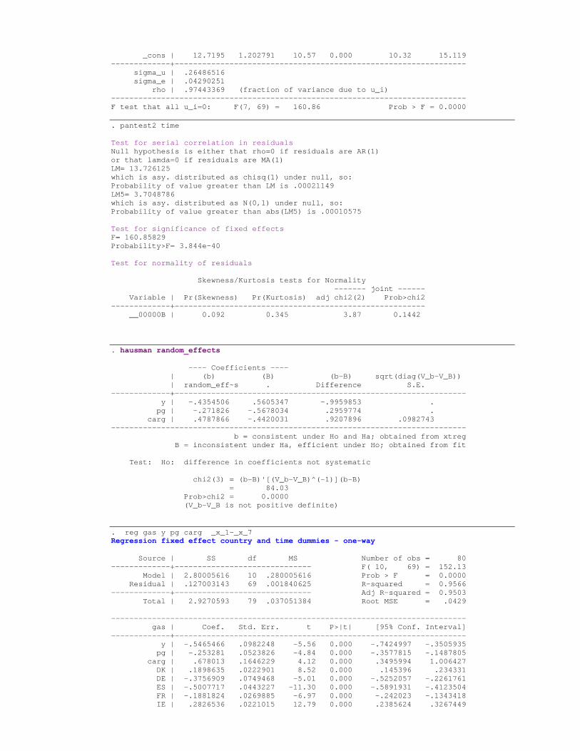
Estimations of the shorter series constructed out of gasoline cars re-

vealed negative income effects and positive gasoline car per capita effect,

which is not in line with prediction. For instance, via the fixed effect model

one gets -0.55, -0.25, 0.68, and 12.72 for output per capita, relative gasoline

price, gasoline car per capita, and the constant, respectively. One possible

explanation for the inverted sign of output is that higher output is strongly

correlated with consumed diesel by trucks for transportation purposes and

not with privately driven kilometers by gasoline cars. Note, that mainly

trucks and passenger road vehicles3 use diesel motors. This possible ef-

fect also appears in the car total constructed series. Note further, that the

fuel demand by private person is very inelastic at least within the current

price range of fuel, so that no dependence on economic output should be

expected. This hypothetical discussion becomes abundant if one looks at

the estimation accounting for serial correlation (see below) where the signs

change.

To explain the effect of positive correlation of gasoline consumption with

car per capita, one has to look at the increasing mobility of the second per-

son in a family household either for work or organizing the household. The

underlying assumption is that the major part of private persons own gaso-

line driven cars which is in line with the data throughout the countries.

However, the diesel motor share is strongly increasing recently4 so conse-

quently one could expect parameter shift also in the Diesel and total car

series estimations.

Next difference to the previous estimation, is the insignificant constant

term over all standard estimation methods. Further, Hausman-test rejects

the null, thus one takes the FE-model. LR- and F-test strongly decide3not to be mixed up with passenger cars (dt. Personenkraftwagen) as it seemed to hap-

pened with the OECD data.4Here I would like to stress again, that due to the explosive increase in Diesel cars (f.i. in

Austria, France, and Belgium) the work suffers a lot from the absence of data from 2002

till now.

6

for two-way FE-model. This model is also an exception to the above said

in so far that output elasticity is positive being in line with the B&Gs’

prediction. The beautyspot of the latter model is the insignificance of the

coefficient of relative gasoline price, because, although generally fuel demand

is strongly inelastic, the households - especially in the first years of the used

data series - mainly use gasoline driven cars and they should react somehow

to increased prices. In contrast, this coefficient is significant in the total

car as well in diesel car estimation. However, the negative coefficient of

the relative gasoline price in the gasoline car estimation becomes significant

after estimating implemented serial correlation.

Looking at the coefficients of the time dummies, except the first they

are all significant and gradually decreasing. The same applies also to the

total car estimation. One explanation could be that efficiency of motor cars

increased over time due to technological innovations. I personally doubt

this. No substantial improvement in motor technology occurred in the last

ten years. Further, increased usage of air condition in cars and more car

overcrowding in cities, which results in more wasteful stop-and-go driving

behaviour, would compensate any efficiency gains by far. The most reason-

able interpretation of the observed gradual decrease of gasoline consumption

over time considers the strong diesel substitution for gasoline which can be

directly read off the data of all countries.

Looking now at the corresponding coefficients of the diesel constructed

series estimation one should observe the opposite. Indeed, one finds - though

all time coefficients are insignificant - a gradual increase over time which

strongly supports the interpretation of the observed effect.

Again one observes serial correlation which is more or less fixed by het-

eroscedasticity adjusted GLS panel estimation provided by STATA. Inter-

estingly again, with some GLS-models the sign of the car per capita effect

changes to the predicted sign by B&G.

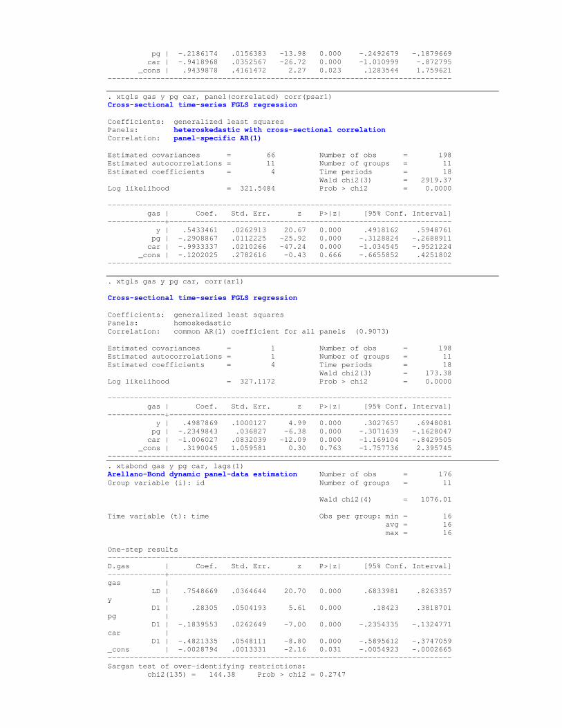
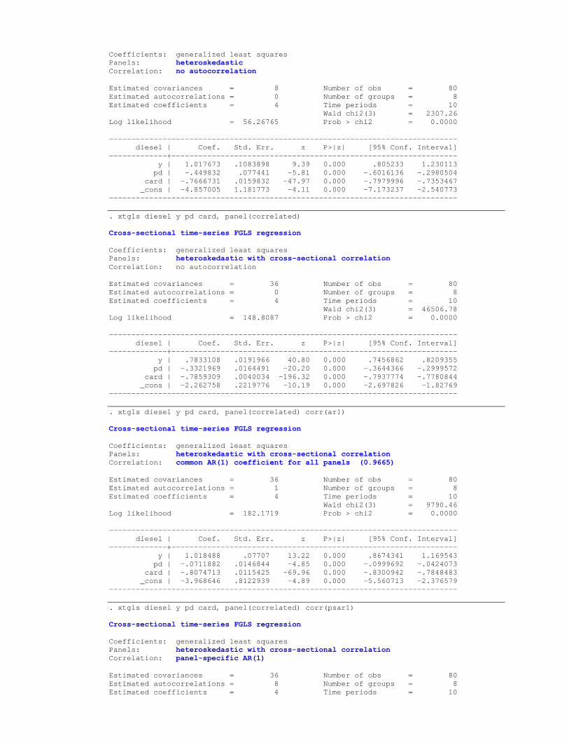
The best estimation is the one with heteroscedastic, cross-sectional cor-

relation, but without autocorrelation in the errors. All coefficients are highly

significant and have predicted sign. As already mentioned, this renders the

above interpretation of the effect of the positive sign of the cars per capita

and of output obsolete. The values for the coefficients are: approx. 0.57,

7

-0.55, -0.44, and -0.54 for output per capita, relative gasoline price, gasoline

cars per capita, and intercept, respectively.

Estimations with differenced and lagged dependent and/or exogenous

regressors did not improve results. Still autocorrelation can be observed.

Addition of regressor relative price of Diesel to gasoline turned out to be

insignificant corresponding to findings of B&G and in our total car estima-

tion.

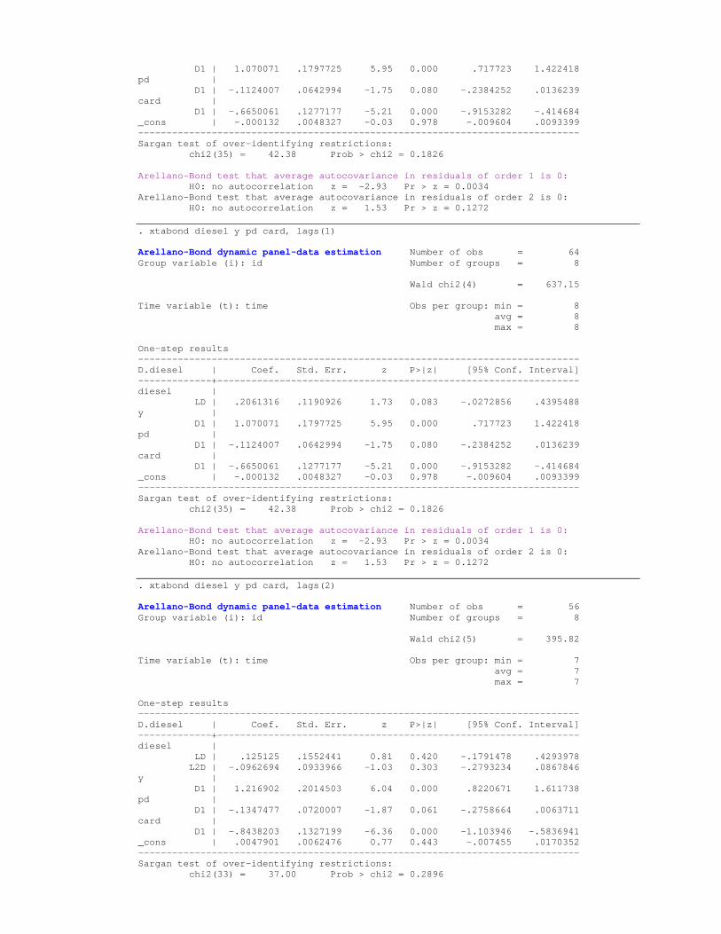
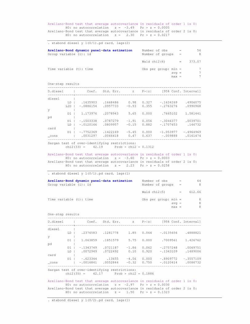
Lastly, I estimated the Diesel car constructed series. The qualitative

results resemble to those of the total car estimation. All coefficients obtain

the predicted sign throughout nearly all types of estimation. The quantita-

tive effects of output and car per capita are larger than those in total car

and gasoline car estimation. The exception is the value of the effect of rela-

tive diesel price which is reasonably smaller compared to the former cases.

This could be again a hint for the substitution effect of diesel combined

with inelastic fuel demand of the individual households and transportation

industry.

Both RE and FE are doing quiet well. R2 within and total is higher than

in the other compared cases. Again, one observes strong serial correlation

given by LM-test. The value of the Hausman-test does clearly not reject the

null. LR-test and F-test prefer the one-way FE to the two-way FE-model.

Looking at the estimation with individual dummies, all countries except

Spain develop lower than Belgium. Each coefficient estimate is significant

except the individual country effect for Ireland.

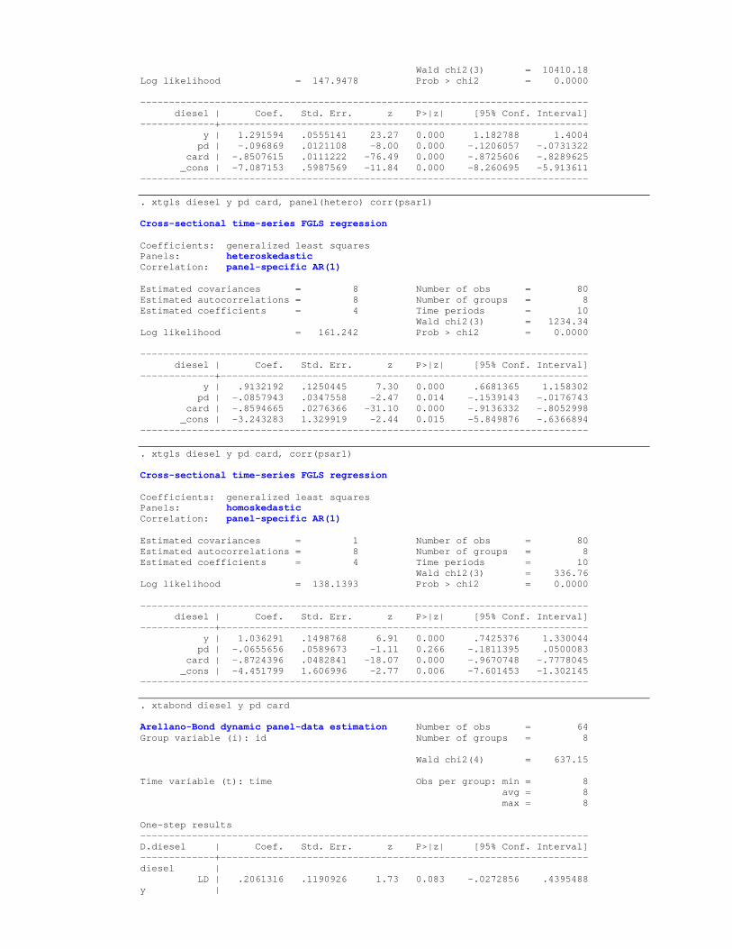
Again, heteroscedastic, cross-sectional correlation adjusted GLS estima-

tion cures the observed serial correlation. The highly significant coefficient

estimates, which are more distinct as in the case of gasoline series, are 0.78,

-0.33, -0.78, and -2.26 for output per capita, relative diesel price, diesel

car per capita, and the constant, respectively. Here, allowing for autocor-

relation of error term improves even further the estimation results in the

panel-specific AR(1)-case as well as in the common case5. In the latter case,

one gets for y, pd, card, and constant 1.018, -0.07, -0.81, and -3.96, respec-

tively. Note, that the impact of a rise in relative diesel price nearly vanishes5Second best estimation is panel-specific AR(1) autocorrelation giving very similar results

8

compared to the one of the gasoline estimation. The first reveals the very

inelastic fuel demand in general, whereas the second reflects the more elastic

diesel-substitution effect.

Taking first differences and lagged dependent and exogenous regressors

could not improve estimation results6.

Again, the coefficient of the included regressor relative diesel price to

gasoline price has been insignificant.

4 Conclusion

The qualitative results of the estimation of the total car series correspond to

those obtained by B&G, which are given in their paper and in the textbook

by Baltagi. In addition, I checked the estimates of the whole B&G-panel as

well as of a truncated version for the sake of comparison with my constructed

panel. The income elasticity is positive, relative price effect is negative,

and effect of increased car ownership is negative on gasoline consumption.

However, all estimations suffer from serious serial correlation as indicated

by tests. This is again in line with the results by B&G. A GLS estimation

with heteroscedastic errors improved the quality, and even more with cross-

section correlation with or without AR(1)-errors in all three investigated

cases. The estimated coefficient of the AR-term seemed to be high. Thus, I

tried estimation with first differences and lagged dependent and exogenous

variables. The results were ambiguous.

The effect of relative price of diesel to gasoline turned out to be insignif-

icant in all cases which corresponds to the results by B&G.

The GLS estimation accounting for heteroscedastic, cross-sectional cor-

relation turned out to be promising for all three investigated types of fuel

demand function. To verify this result, more intensive residual diagnostics

should be undertaken.

What can be improved is the inclusion of countries with shorter time6Especially after taking first differences, the gasoline/diesel car series became too short.

At this point, I have to point out, that I could not manage to run diverse residual

diagnostic packages for the panel estimations in STATA, such that my obtained results

and conclusions are qualified.

9

series so that one deals with unbalanced panels. Also, for future research it

would be interesting to examine similar data but with longer time horizon

and including period 2003 till at least 2005. In this period, we will observe a

sharp increase in oil price which should induce strong effects on the demand

function.

Appendix:

10

Gasoline demand per total cars . xtreg gas y pg car, re Random-effects GLS regression Number of obs = 198 Group variable (i): id Number of groups = 11 R-sq: within = 0.5960 Obs per group: min = 18 between = 0.5561 avg = 18.0 overall = 0.5563 max = 18 Random effects u_i ~ Gaussian Wald chi2(3) = 280.23 corr(u_i, X) = 0 (assumed) Prob > chi2 = 0.0000 ------------------------------------------------------------------------------ gas | Coef. Std. Err. z P>|z| [95% Conf. Interval] -------------+---------------------------------------------------------------- y | .4864349 .0859576 5.66 0.000 .3179611 .6549087 pg | -.5086575 .0403008 -12.62 0.000 -.5876456 -.4296695 car | -1.250908 .093972 -13.31 0.000 -1.43509 -1.066727 _cons | -.4733032 .9834101 -0.48 0.630 -2.400752 1.454145 -------------+---------------------------------------------------------------- sigma_u | .19949125 sigma_e | .08727359 rho | .83935611 (fraction of variance due to u_i) ------------------------------------------------------------------------------ . xttest1 Tests for the error component model: gas[id,t] = Xb + u[id] + v[id,t] v[id,t] = rho v[id,(t-1)] + e[id,t] Estimated results: Var sd = sqrt(Var) ---------+----------------------------- gas | .098387 .3136671 e | .0076167 .08727359 u | .0397968 .19949125 Tests: Random Effects, Two Sided: LM(Var(u)=0) = 891.54 Pr>chi2(1) = 0.0000 ALM(Var(u)=0) = 709.04 Pr>chi2(1) = 0.0000 Random Effects, One Sided: LM(Var(u)=0) = 29.86 Pr>N(0,1) = 0.0000 ALM(Var(u)=0) = 26.63 Pr>N(0,1) = 0.0000 Serial Correlation: LM(rho=0) = 203.38 Pr>chi2(1) = 0.0000 ALM(rho=0) = 20.88 Pr>chi2(1) = 0.0000 Joint Test: LM(Var(u)=0,rho=0) = 912.43 Pr>chi2(2) = 0.0000 . xtreg gas y pg car, fe Fixed-effects (within) regression Number of obs = 198 Group variable (i): id Number of groups = 11 R-sq: within = 0.5961 Obs per group: min = 18 between = 0.5549 avg = 18.0 overall = 0.5553 max = 18 F(3,184) = 90.50 corr(u_i, Xb) = -0.3624 Prob > F = 0.0000 ------------------------------------------------------------------------------ gas | Coef. Std. Err. t P>|t| [95% Conf. Interval] -------------+---------------------------------------------------------------- y | .4906543 .0880458 5.57 0.000 .3169451 .6643635 pg | -.5177339 .0412172 -12.56 0.000 -.599053 -.4364148 car | -1.273783 .0979822 -13.00 0.000 -1.467096 -1.08047

_cons | -.5616356 1.009873 -0.56 0.579 -2.554055 1.430784 -------------+---------------------------------------------------------------- sigma_u | .21485558 sigma_e | .08727359 rho | .85837234 (fraction of variance due to u_i) ------------------------------------------------------------------------------ F test that all u_i=0: F(10, 184) = 83.03 Prob > F = 0.0000 Hausman specification test ---- Coefficients ---- | Fixed Random gas | Effects Effects Difference -------------+----------------------------------------- y | .4906543 .4864349 .0042194 pg | -.5177339 -.5086575 -.0090764 car | -1.273783 -1.250908 -.0228749 Test: Ho: difference in coefficients not systematic chi2( 3) = (b-B)'[S^(-1)](b-B), S = (S_fe - S_re) = 5.36 Prob>chi2 = 0.1474 . reg gas y pg car _x_1-_x_10 Regression fixed effect country and time dummies - one-way Source | SS df MS Number of obs = 198 -------------+------------------------------ F( 13, 184) = 181.59 Model | 17.9807778 13 1.38313675 Prob > F = 0.0000 Residual | 1.40146892 184 .007616679 R-squared = 0.9277 -------------+------------------------------ Adj R-squared = 0.9226 Total | 19.3822467 197 .098387039 Root MSE = .08727 ------------------------------------------------------------------------------ gas | Coef. Std. Err. t P>|t| [95% Conf. Interval] -------------+---------------------------------------------------------------- y | .4906543 .0880458 5.57 0.000 .3169451 .6643635 pg | -.5177339 .0412172 -12.56 0.000 -.599053 -.4364148 car | -1.273783 .0979822 -13.00 0.000 -1.467096 -1.08047 DK | .1594472 .0411584 3.87 0.000 .0782441 .2406503 DE | .3794523 .0343083 11.06 0.000 .311764 .4471405 GR | -.000849 .0500588 -0.02 0.986 -.099612 .0979141 ES | -.1712933 .032681 -5.24 0.000 -.235771 -.1068157 FR | .0924119 .0299217 3.09 0.002 .0333782 .1514455 IE | .0996686 .040401 2.47 0.015 .0199599 .1793773 IT | .1804287 .0416498 4.33 0.000 .0982561 .2626014 NL | -.0554366 .0302994 -1.83 0.069 -.1152155 .0043422 PT | -.3222081 .0367659 -8.76 0.000 -.3947451 -.2496712 UK | .3964964 .0294703 13.45 0.000 .3383532 .4546396 _cons (BE) | -.6305554 1.007996 -0.63 0.532 -2.619271 1.35816 ------------------------------------------------------------------------------ . ereturn list scalars: e(N) = 198 e(df_m) = 13 e(df_r) = 184 e(F) = 181.5931549760814 e(r2) = .9276931647885042 e(rmse) = .0872735865748828 e(mss) = 17.98077780678826 e(rss) = 1.401468920110417 e(r2_a) = .9225845296920398 e(ll) = 209.1740358578644 e(ll_0) = -50.88278899821908 . reg gas y pg car _x_1-_x_27 Regression fixed effect country and time dummies - two-way Source | SS df MS Number of obs = 198 -------------+------------------------------ F( 30, 167) = 89.49 Model | 18.247155 30 .6082385 Prob > F = 0.0000 Residual | 1.13509174 167 .006796957 R-squared = 0.9414 -------------+------------------------------ Adj R-squared = 0.9309

Total | 19.3822467 197 .098387039 Root MSE = .08244 ------------------------------------------------------------------------------ gas | Coef. Std. Err. t P>|t| [95% Conf. Interval] -------------+---------------------------------------------------------------- y | .7569654 .0988987 7.65 0.000 .5617127 .9522182 pg | -.514977 .0504471 -10.21 0.000 -.6145733 -.4153807 car | -1.085439 .1200854 -9.04 0.000 -1.32252 -.848358 DK | .1756457 .0415382 4.23 0.000 .093638 .2576534 DE | .3625091 .0339971 10.66 0.000 .2953896 .4296286 GR | .2526158 .0809674 3.12 0.002 .0927641 .4124674 ES | -.0624024 .0395083 -1.58 0.116 -.1404025 .0155977 FR | .0741538 .0292193 2.54 0.012 .016467 .1318407 IE | .2374178 .0542408 4.38 0.000 .1303317 .3445039 IT | .1401379 .0460565 3.04 0.003 .04921 .2310658 NL | -.0441861 .0289902 -1.52 0.129 -.1014207 .0130485 PT | -.1047926 .060118 -1.74 0.083 -.2234818 .0138967 UK | .4241119 .028776 14.74 0.000 .3673004 .4809235 1986 | -.05987 .0357605 -1.67 0.096 -.1304708 .0107309 1987 | -.1067793 .0367532 -2.91 0.004 -.1793401 -.0342185 1988 | -.1325431 .0379421 -3.49 0.001 -.2074512 -.0576351 1989 | -.1437584 .0386075 -3.72 0.000 -.21998 -.0675368 1990 | -.1555958 .0398061 -3.91 0.000 -.2341838 -.0770077 1991 | -.1402506 .0400833 -3.50 0.001 -.219386 -.0611152 1992 | -.139886 .0410992 -3.40 0.001 -.221027 -.058745 1993 | -.1338625 .0410644 -3.26 0.001 -.2149347 -.0527903 1994 | -.1705733 .0422913 -4.03 0.000 -.2540677 -.0870788 1995 | -.2065542 .0437704 -4.72 0.000 -.2929688 -.1201395 1996 | -.1864064 .0447248 -4.17 0.000 -.2747053 -.0981076 1997 | -.1941772 .0464053 -4.18 0.000 -.2857938 -.1025605 1998 | -.2211569 .0485399 -4.56 0.000 -.3169877 -.125326 1999 | -.2483691 .0508378 -4.89 0.000 -.3487366 -.1480016 2000 | -.2332983 .053748 -4.34 0.000 -.3394114 -.1271852 2001 | -.2763128 .0554089 -4.99 0.000 -.3857049 -.1669207 2002 | -.3208961 .0564938 -5.68 0.000 -.4324303 -.209362 cons(BE,1985)| -2.950763 1.079525 -2.73 0.007 -5.082038 -.8194874 ------------------------------------------------------------------------------ Test for H0: λi=0 , comparing one-way against two-way FE-model LR=2*(230.0439 - 209.174)= 41.74 Chi^2(18) p=0.0012 F = (1.40146 - 1.13509)*183 / 1.13509*10 = 4,294 F(10,183) p=0.00002 . xtgls gas y pg car, panel(hetero) Cross-sectional time-series FGLS regression Coefficients: generalized least squares Panels: heteroskedastic Correlation: no autocorrelation Estimated covariances = 11 Number of obs = 198 Estimated autocorrelations = 0 Number of groups = 11 Estimated coefficients = 4 Time periods = 18 Wald chi2(3) = 2191.41 Log likelihood = 96.344 Prob > chi2 = 0.0000 ------------------------------------------------------------------------------ gas | Coef. Std. Err. z P>|z| [95% Conf. Interval] -------------+---------------------------------------------------------------- y | .8023007 .043241 18.55 0.000 .7175499 .8870514 pg | -.4000542 .0325038 -12.31 0.000 -.4637605 -.3363478 car | -1.219584 .028108 -43.39 0.000 -1.274674 -1.164493 _cons | -3.279778 .4356502 -7.53 0.000 -4.133637 -2.42592 ------------------------------------------------------------------------------ . xtgls gas y pg car, panel(correlated) Cross-sectional time-series FGLS regression Coefficients: generalized least squares Panels: heteroskedastic with cross-sectional correlation Correlation: no autocorrelation Estimated covariances = 66 Number of obs = 198 Estimated autocorrelations = 0 Number of groups = 11

Estimated coefficients = 4 Time periods = 18 Wald chi2(3) = 21192.26 Log likelihood = 349.5028 Prob > chi2 = 0.0000 ------------------------------------------------------------------------------ gas | Coef. Std. Err. z P>|z| [95% Conf. Interval] -------------+---------------------------------------------------------------- y | .7931605 .0091448 86.73 0.000 .775237 .8110841 pg | -.4565131 .0068595 -66.55 0.000 -.4699575 -.4430687 car | -1.156407 .0082692 -139.85 0.000 -1.172614 -1.140199 _cons | -3.276874 .0983149 -33.33 0.000 -3.469568 -3.084181 ------------------------------------------------------------------------------ . xtgls gas y pg car, panel(hetero) corr(ar1) Cross-sectional time-series FGLS regression Coefficients: generalized least squares Panels: heteroskedastic Correlation: common AR(1) coefficient for all panels (0.9073) Estimated covariances = 11 Number of obs = 198 Estimated autocorrelations = 1 Number of groups = 11 Estimated coefficients = 4 Time periods = 18 Wald chi2(3) = 271.76 Log likelihood = 348.6747 Prob > chi2 = 0.0000 ------------------------------------------------------------------------------ gas | Coef. Std. Err. z P>|z| [95% Conf. Interval] -------------+---------------------------------------------------------------- y | .4244021 .0837576 5.07 0.000 .2602402 .588564 pg | -.2168621 .0290442 -7.47 0.000 -.2737877 -.1599365 car | -1.00271 .0676626 -14.82 0.000 -1.135327 -.8700942 _cons | 1.134649 .8936769 1.27 0.204 -.6169254 2.886224 ------------------------------------------------------------------------------ . xtgls gas y pg car, panel(hetero) corr(psar1) Cross-sectional time-series FGLS regression Coefficients: generalized least squares Panels: heteroskedastic Correlation: panel-specific AR(1) Estimated covariances = 11 Number of obs = 198 Estimated autocorrelations = 11 Number of groups = 11 Estimated coefficients = 4 Time periods = 18 Wald chi2(3) = 823.87 Log likelihood = 378.7658 Prob > chi2 = 0.0000 ------------------------------------------------------------------------------ gas | Coef. Std. Err. z P>|z| [95% Conf. Interval] -------------+---------------------------------------------------------------- y | .5663818 .0504493 11.23 0.000 .4675029 .6652606 pg | -.2842756 .0223492 -12.72 0.000 -.3280792 -.240472 car | -1.092482 .0410568 -26.61 0.000 -1.172952 -1.012012 _cons | -.4742299 .542888 -0.87 0.382 -1.538271 .5898111 ------------------------------------------------------------------------------ . xtgls gas y pg car, panel(correlated) corr(ar1) Cross-sectional time-series FGLS regression Coefficients: generalized least squares Panels: heteroskedastic with cross-sectional correlation Correlation: common AR(1) coefficient for all panels (0.9073) Estimated covariances = 66 Number of obs = 198 Estimated autocorrelations = 1 Number of groups = 11 Estimated coefficients = 4 Time periods = 18 Wald chi2(3) = 829.62 Log likelihood = 434.1516 Prob > chi2 = 0.0000 ------------------------------------------------------------------------------ gas | Coef. Std. Err. z P>|z| [95% Conf. Interval] -------------+---------------------------------------------------------------- y | .4489298 .038502 11.66 0.000 .3734673 .5243922

pg | -.2186174 .0156383 -13.98 0.000 -.2492679 -.1879669 car | -.9418968 .0352567 -26.72 0.000 -1.010999 -.872795 _cons | .9439878 .4161472 2.27 0.023 .1283544 1.759621 ------------------------------------------------------------------------------ . xtgls gas y pg car, panel(correlated) corr(psar1) Cross-sectional time-series FGLS regression Coefficients: generalized least squares Panels: heteroskedastic with cross-sectional correlation Correlation: panel-specific AR(1) Estimated covariances = 66 Number of obs = 198 Estimated autocorrelations = 11 Number of groups = 11 Estimated coefficients = 4 Time periods = 18 Wald chi2(3) = 2919.37 Log likelihood = 321.5484 Prob > chi2 = 0.0000 ------------------------------------------------------------------------------ gas | Coef. Std. Err. z P>|z| [95% Conf. Interval] -------------+---------------------------------------------------------------- y | .5433461 .0262913 20.67 0.000 .4918162 .5948761 pg | -.2908867 .0112225 -25.92 0.000 -.3128824 -.2688911 car | -.9933337 .0210266 -47.24 0.000 -1.034545 -.9521224 _cons | -.1202025 .2782616 -0.43 0.666 -.6655852 .4251802 ------------------------------------------------------------------------------ . xtgls gas y pg car, corr(ar1) Cross-sectional time-series FGLS regression Coefficients: generalized least squares Panels: homoskedastic Correlation: common AR(1) coefficient for all panels (0.9073) Estimated covariances = 1 Number of obs = 198 Estimated autocorrelations = 1 Number of groups = 11 Estimated coefficients = 4 Time periods = 18 Wald chi2(3) = 173.38 Log likelihood = 327.1172 Prob > chi2 = 0.0000 ------------------------------------------------------------------------------ gas | Coef. Std. Err. z P>|z| [95% Conf. Interval] -------------+---------------------------------------------------------------- y | .4987869 .1000127 4.99 0.000 .3027657 .6948081 pg | -.2349843 .036827 -6.38 0.000 -.3071639 -.1628047 car | -1.006027 .0832039 -12.09 0.000 -1.169104 -.8429505 _cons | .3190045 1.059581 0.30 0.763 -1.757736 2.395745 ------------------------------------------------------------------------------ . xtabond gas y pg car, lags(1) Arellano-Bond dynamic panel-data estimation Number of obs = 176 Group variable (i): id Number of groups = 11 Wald chi2(4) = 1076.01 Time variable (t): time Obs per group: min = 16 avg = 16 max = 16 One-step results ------------------------------------------------------------------------------ D.gas | Coef. Std. Err. z P>|z| [95% Conf. Interval] -------------+---------------------------------------------------------------- gas | LD | .7548669 .0364644 20.70 0.000 .6833981 .8263357 y | D1 | .28305 .0504193 5.61 0.000 .18423 .3818701 pg | D1 | -.1839553 .0262649 -7.00 0.000 -.2354335 -.1324771 car | D1 | -.4821335 .0548111 -8.80 0.000 -.5895612 -.3747059 _cons | -.0028794 .0013331 -2.16 0.031 -.0054923 -.0002665 ------------------------------------------------------------------------------ Sargan test of over-identifying restrictions: chi2(135) = 144.38 Prob > chi2 = 0.2747

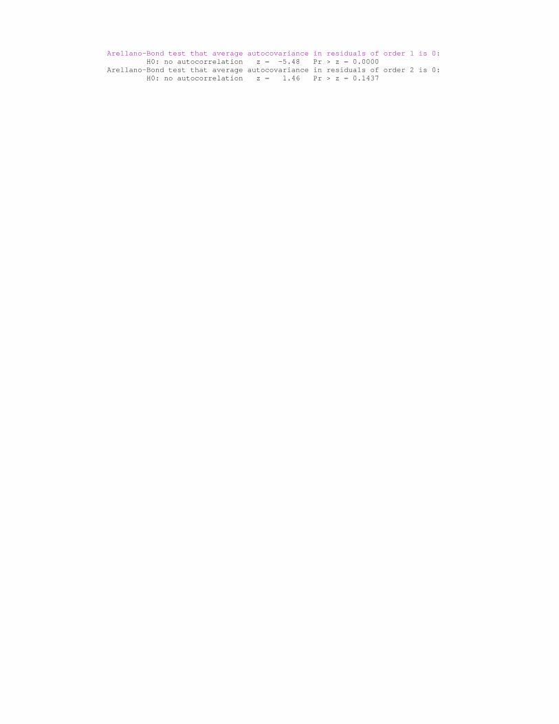
Arellano-Bond test that average autocovariance in residuals of order 1 is 0: H0: no autocorrelation z = -5.48 Pr > z = 0.0000 Arellano-Bond test that average autocovariance in residuals of order 2 is 0: H0: no autocorrelation z = 1.46 Pr > z = 0.1437

Gasoline demand per gasoline car . xtreg gas y pg carg, re Random-effects GLS regression Number of obs = 80 Group variable (i): id Number of groups = 8 R-sq: within = 0.5464 Obs per group: min = 10 between = 0.1285 avg = 10.0 overall = 0.0420 max = 10 Random effects u_i ~ Gaussian Wald chi2(3) = 67.90 corr(u_i, X) = 0 (assumed) Prob > chi2 = 0.0000 ------------------------------------------------------------------------------ gas | Coef. Std. Err. z P>|z| [95% Conf. Interval] -------------+---------------------------------------------------------------- y | -.4354506 .0985217 -4.42 0.000 -.6285497 -.2423515 pg | -.271826 .0557396 -4.88 0.000 -.3810735 -.1625785 carg | .4787866 .1617361 2.96 0.003 .1617896 .7957836 _cons | 11.33054 1.202541 9.42 0.000 8.9736 13.68747 -------------+---------------------------------------------------------------- sigma_u | .15469492 sigma_e | .04290251 rho | .92857806 (fraction of variance due to u_i) ------------------------------------------------------------------------------ . xttest1 Tests for the error component model: gas[id,t] = Xb + u[id] + v[id,t] v[id,t] = rho v[id,(t-1)] + e[id,t] Estimated results: Var sd = sqrt(Var) ---------+----------------------------- gas | .0370514 .1924874 e | .0018406 .04290251 u | .0239305 .15469492 Tests: Random Effects, Two Sided: LM(Var(u)=0) = 221.19 Pr>chi2(1) = 0.0000 ALM(Var(u)=0) = 149.77 Pr>chi2(1) = 0.0000 Random Effects, One Sided: LM(Var(u)=0) = 14.87 Pr>N(0,1) = 0.0000 ALM(Var(u)=0) = 12.24 Pr>N(0,1) = 0.0000 Serial Correlation: LM(rho=0) = 77.07 Pr>chi2(1) = 0.0000 ALM(rho=0) = 5.66 Pr>chi2(1) = 0.0173 Joint Test: LM(Var(u)=0,rho=0) = 226.85 Pr>chi2(2) = 0.0000 . xtreg gas y pg carg, fe Fixed-effects (within) regression Number of obs = 80 Group variable (i): id Number of groups = 8 R-sq: within = 0.5545 Obs per group: min = 10 between = 0.1524 avg = 10.0 overall = 0.0669 max = 10 F(3,69) = 28.62 corr(u_i, Xb) = -0.6854 Prob > F = 0.0000 ------------------------------------------------------------------------------ gas | Coef. Std. Err. t P>|t| [95% Conf. Interval] -------------+---------------------------------------------------------------- y | -.5465466 .0982248 -5.56 0.000 -.7424997 -.3505935 pg | -.253281 .0523826 -4.84 0.000 -.3577815 -.1487805 carg | .678013 .1646229 4.12 0.000 .3495994 1.006427

_cons | 12.7195 1.202791 10.57 0.000 10.32 15.119 -------------+---------------------------------------------------------------- sigma_u | .26486516 sigma_e | .04290251 rho | .97443369 (fraction of variance due to u_i) ------------------------------------------------------------------------------ F test that all u_i=0: F(7, 69) = 160.86 Prob > F = 0.0000 . pantest2 time Test for serial correlation in residuals Null hypothesis is either that rho=0 if residuals are AR(1) or that lamda=0 if residuals are MA(1) LM= 13.726125 which is asy. distributed as chisq(1) under null, so: Probability of value greater than LM is .00021149 LM5= 3.7048786 which is asy. distributed as N(0,1) under null, so: Probability of value greater than abs(LM5) is .00010575 Test for significance of fixed effects F= 160.85829 Probability>F= 3.844e-40 Test for normality of residuals Skewness/Kurtosis tests for Normality ------- joint ------ Variable | Pr(Skewness) Pr(Kurtosis) adj chi2(2) Prob>chi2 -------------+------------------------------------------------------- __00000B | 0.092 0.345 3.87 0.1442 . hausman random_effects ---- Coefficients ---- | (b) (B) (b-B) sqrt(diag(V_b-V_B)) | random_eff~s . Difference S.E. -------------+---------------------------------------------------------------- y | -.4354506 .5605347 -.9959853 . pg | -.271826 -.5678034 .2959774 . carg | .4787866 -.4420031 .9207896 .0982743 ------------------------------------------------------------------------------ b = consistent under Ho and Ha; obtained from xtreg B = inconsistent under Ha, efficient under Ho; obtained from fit Test: Ho: difference in coefficients not systematic chi2(3) = (b-B)'[(V_b-V_B)^(-1)](b-B) = 84.03 Prob>chi2 = 0.0000 (V_b-V_B is not positive definite) . reg gas y pg carg _x_1-_x_7 Regression fixed effect country and time dummies - one-way Source | SS df MS Number of obs = 80 -------------+------------------------------ F( 10, 69) = 152.13 Model | 2.80005616 10 .280005616 Prob > F = 0.0000 Residual | .127003143 69 .001840625 R-squared = 0.9566 -------------+------------------------------ Adj R-squared = 0.9503 Total | 2.9270593 79 .037051384 Root MSE = .0429 ------------------------------------------------------------------------------ gas | Coef. Std. Err. t P>|t| [95% Conf. Interval] -------------+---------------------------------------------------------------- y | -.5465466 .0982248 -5.56 0.000 -.7424997 -.3505935 pg | -.253281 .0523826 -4.84 0.000 -.3577815 -.1487805 carg | .678013 .1646229 4.12 0.000 .3495994 1.006427 DK | .1898635 .0222901 8.52 0.000 .145396 .234331 DE | -.3756909 .0749468 -5.01 0.000 -.5252057 -.2261761 ES | -.5007717 .0443227 -11.30 0.000 -.5891931 -.4123504 FR | -.1881824 .0269885 -6.97 0.000 -.242023 -.1343418 IE | .2826536 .0221015 12.79 0.000 .2385624 .3267449

NL | -.130084 .0254658 -5.11 0.000 -.1808869 -.079281 UK | -.0246434 .0463584 -0.53 0.597 -.1171257 .067839 _cons (BE) | 12.81285 1.224575 10.46 0.000 10.36989 15.25582 ------------------------------------------------------------------------------ . reg gas y pg carg _x_1-_x_16 Regression fixed effect country and time dummies - two-way Source | SS df MS Number of obs = 80 -------------+------------------------------ F( 19, 60) = 151.08 Model | 2.86712933 19 .150901544 Prob > F = 0.0000 Residual | .059929971 60 .000998833 R-squared = 0.9795 -------------+------------------------------ Adj R-squared = 0.9730 Total | 2.9270593 79 .037051384 Root MSE = .0316 ------------------------------------------------------------------------------ gas | Coef. Std. Err. t P>|t| [95% Conf. Interval] -------------+---------------------------------------------------------------- y | .2377113 .1249086 1.90 0.062 -.012143 .4875657 pg | -.0280023 .0525213 -0.53 0.596 -.1330604 .0770559 carg | .2817035 .1328165 2.12 0.038 .0160311 .547376 DK | .1715972 .0166213 10.32 0.000 .1383496 .2048447 DE | -.19406 .0604912 -3.21 0.002 -.3150603 -.0730596 ES | -.2016587 .0513565 -3.93 0.000 -.304387 -.0989305 FR | -.1658507 .0201753 -8.22 0.000 -.2062074 -.1254941 IE | .3703215 .0202251 18.31 0.000 .3298652 .4107778 NL | -.1292135 .0188747 -6.85 0.000 -.1669685 -.0914586 UK | .1145693 .0389181 2.94 0.005 .0367215 .1924171 1993 | -.0065026 .0158603 -0.41 0.683 -.0382279 .0252228 1994 | -.0346571 .0160024 -2.17 0.034 -.0666666 -.0026475 1995 | -.0710464 .0165252 -4.30 0.000 -.1041016 -.0379911 1996 | -.0769266 .0172494 -4.46 0.000 -.1114306 -.0424227 1997 | -.1124696 .0194845 -5.77 0.000 -.1514445 -.0734948 1998 | -.1307355 .0206819 -6.32 0.000 -.1721056 -.0893655 1999 | -.154687 .0228196 -6.78 0.000 -.200333 -.1090411 2000 | -.1992731 .0296594 -6.72 0.000 -.2586007 -.1399454 2001 | -.2320162 .0297251 -7.81 0.000 -.2914752 -.1725571 cons(BE,1992)| 5.071888 1.348706 3.76 0.000 2.374074 7.769702 ------------------------------------------------------------------------------ Test for H0: λi=0 , comparing one-way against two-way FE-model LR= 2*( 174.349 - 144.307) = 60,08 Chi^2(10) p=0.00000 F= (0.1270 - 0.0599) * 68/0.0599 *7 = 10,88 F(7,68) p=0.00000 . xtgls gas y pg carg Cross-sectional time-series FGLS regression Coefficients: generalized least squares Panels: homoskedastic Correlation: no autocorrelation Estimated covariances = 1 Number of obs = 80 Estimated autocorrelations = 0 Number of groups = 8 Estimated coefficients = 4 Time periods = 10 Wald chi2(3) = 26.46 Log likelihood = 30.23565 Prob > chi2 = 0.0000 ------------------------------------------------------------------------------ gas | Coef. Std. Err. z P>|z| [95% Conf. Interval] -------------+---------------------------------------------------------------- y | .5605347 .1580728 3.55 0.000 .2507177 .8703516 pg | -.5678034 .1627194 -3.49 0.000 -.8867275 -.2488793 carg | -.4420031 .1252026 -3.53 0.000 -.6873957 -.1966104 _cons | -.4590795 1.861315 -0.25 0.805 -4.10719 3.189032 ------------------------------------------------------------------------------ . xtgls gas y pg carg, panel(hetero) Cross-sectional time-series FGLS regression Coefficients: generalized least squares Panels: heteroskedastic Correlation: no autocorrelation Estimated covariances = 8 Number of obs = 80

Estimated autocorrelations = 0 Number of groups = 8 Estimated coefficients = 4 Time periods = 10 Wald chi2(3) = 60.02 Log likelihood = 49.38727 Prob > chi2 = 0.0000 ------------------------------------------------------------------------------ gas | Coef. Std. Err. z P>|z| [95% Conf. Interval] -------------+---------------------------------------------------------------- y | .5186168 .1682102 3.08 0.002 .1889309 .8483028 pg | -.9425805 .1538007 -6.13 0.000 -1.244024 -.6411367 carg | -.2917766 .0686774 -4.25 0.000 -.4263817 -.1571714 _cons | -.8040832 1.932866 -0.42 0.677 -4.592432 2.984265 ------------------------------------------------------------------------------ . xtgls gas y pg carg, panel(correlated) Cross-sectional time-series FGLS regression Coefficients: generalized least squares Panels: heteroskedastic with cross-sectional correlation Correlation: no autocorrelation Estimated covariances = 36 Number of obs = 80 Estimated autocorrelations = 0 Number of groups = 8 Estimated coefficients = 4 Time periods = 10 Wald chi2(3) = 5987.24 Log likelihood = 158.9458 Prob > chi2 = 0.0000 ------------------------------------------------------------------------------ gas | Coef. Std. Err. z P>|z| [95% Conf. Interval] -------------+---------------------------------------------------------------- y | .5731473 .0248694 23.05 0.000 .5244041 .6218905 pg | -.5477575 .0182347 -30.04 0.000 -.5834968 -.5120181 carg | -.4440043 .0070595 -62.89 0.000 -.4578408 -.4301679 _cons | -.537192 .2443208 -2.20 0.028 -1.016052 -.0583321 ------------------------------------------------------------------------------ . xtgls gas y pg carg, panel(hetero) corr(ar1) Cross-sectional time-series FGLS regression Coefficients: generalized least squares Panels: heteroskedastic Correlation: common AR(1) coefficient for all panels (0.9837) Estimated covariances = 8 Number of obs = 80 Estimated autocorrelations = 1 Number of groups = 8 Estimated coefficients = 4 Time periods = 10 Wald chi2(3) = 24.91 Log likelihood = 164.1461 Prob > chi2 = 0.0000 ------------------------------------------------------------------------------ gas | Coef. Std. Err. z P>|z| [95% Conf. Interval] -------------+---------------------------------------------------------------- y | -.2378287 .1415885 -1.68 0.093 -.5153369 .0396796 pg | -.1682994 .0488197 -3.45 0.001 -.2639842 -.0726146 carg | -.1083424 .1992829 -0.54 0.587 -.4989297 .282245 _cons | 8.96812 1.606769 5.58 0.000 5.81891 12.11733 ------------------------------------------------------------------------------ . xtgls gas y pg carg, panel(correlated) corr(ar1) Cross-sectional time-series FGLS regression Coefficients: generalized least squares Panels: heteroskedastic with cross-sectional correlation Correlation: common AR(1) coefficient for all panels (0.9837) Estimated covariances = 36 Number of obs = 80 Estimated autocorrelations = 1 Number of groups = 8 Estimated coefficients = 4 Time periods = 10 Wald chi2(3) = 114.90 Log likelihood = 192.1598 Prob > chi2 = 0.0000 ------------------------------------------------------------------------------ gas | Coef. Std. Err. z P>|z| [95% Conf. Interval] -------------+----------------------------------------------------------------

y | -.2187017 .0686892 -3.18 0.001 -.3533301 -.0840733 pg | -.1703586 .0186207 -9.15 0.000 -.2068546 -.1338626 carg | -.01044 .080193 -0.13 0.896 -.1676154 .1467354 _cons | 8.852241 .7655903 11.56 0.000 7.351712 10.35277 ------------------------------------------------------------------------------ . xtgls gas y pg carg, panel(correlated) corr(psar1) Cross-sectional time-series FGLS regression Coefficients: generalized least squares Panels: heteroskedastic with cross-sectional correlation Correlation: panel-specific AR(1) Estimated covariances = 36 Number of obs = 80 Estimated autocorrelations = 8 Number of groups = 8 Estimated coefficients = 4 Time periods = 10 Wald chi2(3) = 758.40 Log likelihood = 155.0019 Prob > chi2 = 0.0000 ------------------------------------------------------------------------------ gas | Coef. Std. Err. z P>|z| [95% Conf. Interval] -------------+---------------------------------------------------------------- y | .1331203 .0384813 3.46 0.001 .0576985 .2085422 pg | -.2080793 .013864 -15.01 0.000 -.2352523 -.1809063 carg | -.5543796 .0363142 -15.27 0.000 -.6255542 -.483205 _cons | 4.774339 .4183465 11.41 0.000 3.954395 5.594283 ------------------------------------------------------------------------------ . xtgls gas y pg carg, corr(ar1) Cross-sectional time-series FGLS regression Coefficients: generalized least squares Panels: homoskedastic Correlation: common AR(1) coefficient for all panels (0.9837) Estimated covariances = 1 Number of obs = 80 Estimated autocorrelations = 1 Number of groups = 8 Estimated coefficients = 4 Time periods = 10 Wald chi2(3) = 12.24 Log likelihood = 156.3345 Prob > chi2 = 0.0066 ------------------------------------------------------------------------------ gas | Coef. Std. Err. z P>|z| [95% Conf. Interval] -------------+---------------------------------------------------------------- y | -.2386033 .1528398 -1.56 0.118 -.5381638 .0609571 pg | -.128791 .0570698 -2.26 0.024 -.2406458 -.0169362 carg | -.0407414 .2253566 -0.18 0.857 -.4824322 .4009494 _cons | 9.116903 1.755682 5.19 0.000 5.675829 12.55798 ------------------------------------------------------------------------------ . xtabond gas y pg carg, lags(1) Arellano-Bond dynamic panel-data estimation Number of obs = 64 Group variable (i): id Number of groups = 8 Wald chi2(4) = 43.39 Time variable (t): time Obs per group: min = 8 avg = 8 max = 8 One-step results ------------------------------------------------------------------------------ D.gas | Coef. Std. Err. z P>|z| [95% Conf. Interval] -------------+---------------------------------------------------------------- gas | LD | .3246483 .1779284 1.82 0.068 -.0240849 .6733816 y | D1 | .1098794 .173232 0.63 0.526 -.2296491 .449408 pg | D1 | -.1153381 .0503915 -2.29 0.022 -.2141035 -.0165726 carg | D1 | .2428223 .1923124 1.26 0.207 -.134103 .6197476 _cons | -.0160055 .0060226 -2.66 0.008 -.0278096 -.0042013

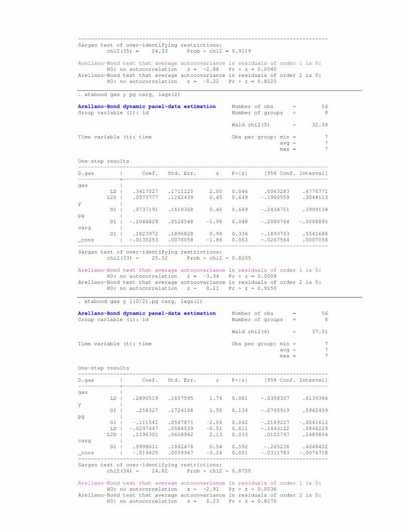
------------------------------------------------------------------------------ Sargan test of over-identifying restrictions: chi2(35) = 24.33 Prob > chi2 = 0.9119 Arellano-Bond test that average autocovariance in residuals of order 1 is 0: H0: no autocorrelation z = -2.88 Pr > z = 0.0040 Arellano-Bond test that average autocovariance in residuals of order 2 is 0: H0: no autocorrelation z = -0.22 Pr > z = 0.8225 . xtabond gas y pg carg, lags(2) Arellano-Bond dynamic panel-data estimation Number of obs = 56 Group variable (i): id Number of groups = 8 Wald chi2(5) = 32.34 Time variable (t): time Obs per group: min = 7 avg = 7 max = 7 One-step results ------------------------------------------------------------------------------ D.gas | Coef. Std. Err. z P>|z| [95% Conf. Interval] -------------+---------------------------------------------------------------- gas | LD | .3417027 .1711125 2.00 0.046 .0063283 .6770771 L2D | .0573777 .1262439 0.45 0.649 -.1900559 .3048113 y | D1 | .0737191 .1618368 0.46 0.649 -.2434751 .3909134 pg | D1 | -.1044829 .0528548 -1.98 0.048 -.2080764 -.0008895 carg | D1 | .1823972 .1896828 0.96 0.336 -.1893743 .5541688 _cons | -.0130253 .0070058 -1.86 0.063 -.0267564 .0007058 ------------------------------------------------------------------------------ Sargan test of over-identifying restrictions: chi2(33) = 25.52 Prob > chi2 = 0.8205 Arellano-Bond test that average autocovariance in residuals of order 1 is 0: H0: no autocorrelation z = -3.34 Pr > z = 0.0008 Arellano-Bond test that average autocovariance in residuals of order 2 is 0: H0: no autocorrelation z = 0.11 Pr > z = 0.9150 . xtabond gas y l(0/2).pg carg, lags(1) Arellano-Bond dynamic panel-data estimation Number of obs = 56 Group variable (i): id Number of groups = 8 Wald chi2(6) = 37.01 Time variable (t): time Obs per group: min = 7 avg = 7 max = 7 One-step results ------------------------------------------------------------------------------ D.gas | Coef. Std. Err. z P>|z| [95% Conf. Interval] -------------+---------------------------------------------------------------- gas | LD | .2890519 .1657595 1.74 0.081 -.0358307 .6139346 y | D1 | .258327 .1724108 1.50 0.134 -.0795919 .5962459 pg | D1 | -.111542 .0547871 -2.04 0.042 -.2189227 -.0041612 LD | -.0297447 .0584539 -0.51 0.611 -.1443122 .0848229 L2D | .1296301 .0608942 2.13 0.033 .0102797 .2489804 carg | D1 | .0998011 .1862478 0.54 0.592 -.265238 .4648402 _cons | -.019425 .0059967 -3.24 0.001 -.0311783 -.0076718 ------------------------------------------------------------------------------ Sargan test of over-identifying restrictions: chi2(34) = 24.82 Prob > chi2 = 0.8750 Arellano-Bond test that average autocovariance in residuals of order 1 is 0: H0: no autocorrelation z = -2.91 Pr > z = 0.0036 Arellano-Bond test that average autocovariance in residuals of order 2 is 0: H0: no autocorrelation z = 0.23 Pr > z = 0.8170

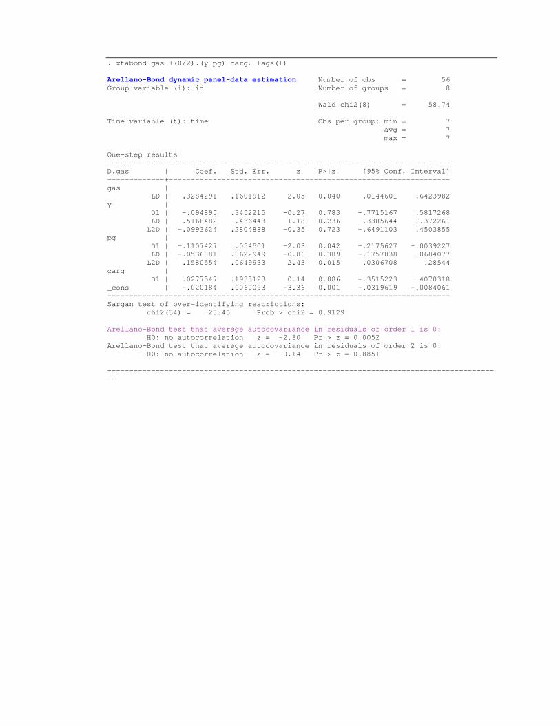
. xtabond gas l(0/2).(y pg) carg, lags(1) Arellano-Bond dynamic panel-data estimation Number of obs = 56 Group variable (i): id Number of groups = 8 Wald chi2(8) = 58.74 Time variable (t): time Obs per group: min = 7 avg = 7 max = 7 One-step results ------------------------------------------------------------------------------ D.gas | Coef. Std. Err. z P>|z| [95% Conf. Interval] -------------+---------------------------------------------------------------- gas | LD | .3284291 .1601912 2.05 0.040 .0144601 .6423982 y | D1 | -.094895 .3452215 -0.27 0.783 -.7715167 .5817268 LD | .5168482 .436443 1.18 0.236 -.3385644 1.372261 L2D | -.0993624 .2804888 -0.35 0.723 -.6491103 .4503855 pg | D1 | -.1107427 .054501 -2.03 0.042 -.2175627 -.0039227 LD | -.0536881 .0622949 -0.86 0.389 -.1757838 .0684077 L2D | .1580554 .0649933 2.43 0.015 .0306708 .28544 carg | D1 | .0277547 .1935123 0.14 0.886 -.3515223 .4070318 _cons | -.020184 .0060093 -3.36 0.001 -.0319619 -.0084061 ------------------------------------------------------------------------------ Sargan test of over-identifying restrictions: chi2(34) = 23.45 Prob > chi2 = 0.9129 Arellano-Bond test that average autocovariance in residuals of order 1 is 0: H0: no autocorrelation z = -2.80 Pr > z = 0.0052 Arellano-Bond test that average autocovariance in residuals of order 2 is 0: H0: no autocorrelation z = 0.14 Pr > z = 0.8851 ------------------------------------------------------------------------------------------

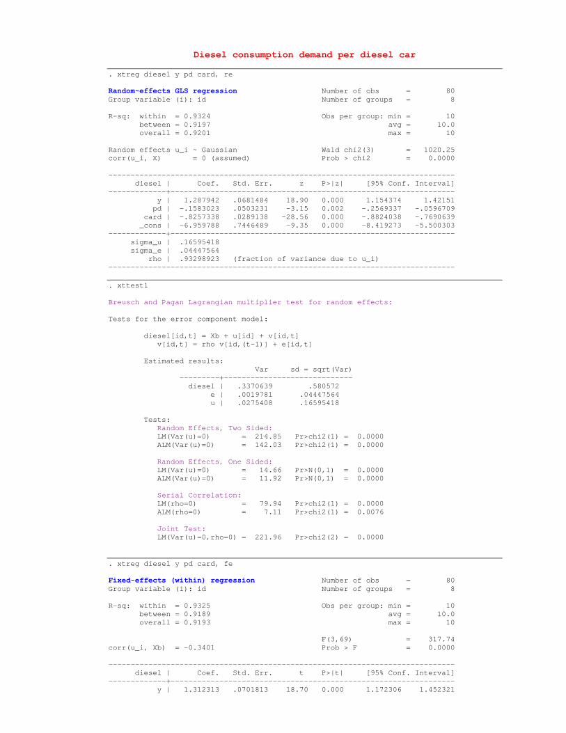
Diesel consumption demand per diesel car . xtreg diesel y pd card, re Random-effects GLS regression Number of obs = 80 Group variable (i): id Number of groups = 8 R-sq: within = 0.9324 Obs per group: min = 10 between = 0.9197 avg = 10.0 overall = 0.9201 max = 10 Random effects u_i ~ Gaussian Wald chi2(3) = 1020.25 corr(u_i, X) = 0 (assumed) Prob > chi2 = 0.0000 ------------------------------------------------------------------------------ diesel | Coef. Std. Err. z P>|z| [95% Conf. Interval] -------------+---------------------------------------------------------------- y | 1.287942 .0681484 18.90 0.000 1.154374 1.42151 pd | -.1583023 .0503231 -3.15 0.002 -.2569337 -.0596709 card | -.8257338 .0289138 -28.56 0.000 -.8824038 -.7690639 _cons | -6.959788 .7446489 -9.35 0.000 -8.419273 -5.500303 -------------+---------------------------------------------------------------- sigma_u | .16595418 sigma_e | .04447564 rho | .93298923 (fraction of variance due to u_i) ------------------------------------------------------------------------------ . xttest1 Breusch and Pagan Lagrangian multiplier test for random effects: Tests for the error component model: diesel[id,t] = Xb + u[id] + v[id,t] v[id,t] = rho v[id,(t-1)] + e[id,t] Estimated results: Var sd = sqrt(Var) ---------+----------------------------- diesel | .3370639 .580572 e | .0019781 .04447564 u | .0275408 .16595418 Tests: Random Effects, Two Sided: LM(Var(u)=0) = 214.85 Pr>chi2(1) = 0.0000 ALM(Var(u)=0) = 142.03 Pr>chi2(1) = 0.0000 Random Effects, One Sided: LM(Var(u)=0) = 14.66 Pr>N(0,1) = 0.0000 ALM(Var(u)=0) = 11.92 Pr>N(0,1) = 0.0000 Serial Correlation: LM(rho=0) = 79.94 Pr>chi2(1) = 0.0000 ALM(rho=0) = 7.11 Pr>chi2(1) = 0.0076 Joint Test: LM(Var(u)=0,rho=0) = 221.96 Pr>chi2(2) = 0.0000 . xtreg diesel y pd card, fe Fixed-effects (within) regression Number of obs = 80 Group variable (i): id Number of groups = 8 R-sq: within = 0.9325 Obs per group: min = 10 between = 0.9189 avg = 10.0 overall = 0.9193 max = 10 F(3,69) = 317.74 corr(u_i, Xb) = -0.3401 Prob > F = 0.0000 ------------------------------------------------------------------------------ diesel | Coef. Std. Err. t P>|t| [95% Conf. Interval] -------------+---------------------------------------------------------------- y | 1.312313 .0701813 18.70 0.000 1.172306 1.452321

pd | -.1481031 .0507667 -2.92 0.005 -.2493799 -.0468263 card | -.8371178 .0307916 -27.19 0.000 -.8985453 -.7756903 _cons | -7.208604 .7627813 -9.45 0.000 -8.730311 -5.686897 -------------+---------------------------------------------------------------- sigma_u | .18033059 sigma_e | .04447564 rho | .94265963 (fraction of variance due to u_i) ------------------------------------------------------------------------------ F test that all u_i=0: F(7, 69) = 113.29 Prob > F = 0.0000 . hausman random_effects ---- Coefficients ---- | (b) (B) (b-B) sqrt(diag(V_b-V_B)) | random_eff~s . Difference S.E. -------------+---------------------------------------------------------------- y | 1.287942 1.312313 -.0243715 . pd | -.1583023 -.1481031 -.0101992 . card | -.8257338 -.8371178 .0113839 . ------------------------------------------------------------------------------ b = consistent under Ho and Ha; obtained from xtreg B = inconsistent under Ha, efficient under Ho; obtained from xtreg Test: Ho: difference in coefficients not systematic chi2(3) = (b-B)'[(V_b-V_B)^(-1)](b-B) = 1.22 Prob>chi2 = 0.7490 (V_b-V_B is not positive definite) . pantest2 time Test for serial correlation in residuals Null hypothesis is either that rho=0 if residuals are AR(1) or that lamda=0 if residuals are MA(1) LM= 7.1872079 which is asy. distributed as chisq(1) under null, so: Probability of value greater than LM is .00734251 LM5= 2.6808969 which is asy. distributed as N(0,1) under null, so: Probability of value greater than abs(LM5) is .00367126 Test for significance of fixed effects F= 113.28916 Probability>F= 2.841e-35 Test for normality of residuals Skewness/Kurtosis tests for Normality ------- joint ------ Variable | Pr(Skewness) Pr(Kurtosis) adj chi2(2) Prob>chi2 -------------+------------------------------------------------------- __00000B | 0.078 0.202 4.74 0.0934 . reg diesel y pd card _x_1-_x_7 Regression fixed effect country and time dummies – one-way Source | SS df MS Number of obs = 80 -------------+------------------------------ F( 10, 69) = 1339.25 Model | 26.4915591 10 2.64915591 Prob > F = 0.0000 Residual | .136487683 69 .001978082 R-squared = 0.9949 -------------+------------------------------ Adj R-squared = 0.9941 Total | 26.6280468 79 .337063884 Root MSE = .04448 ------------------------------------------------------------------------------ diesel | Coef. Std. Err. t P>|t| [95% Conf. Interval] -------------+---------------------------------------------------------------- y | 1.312313 .0701813 18.70 0.000 1.172306 1.452321 pd | -.1481031 .0507667 -2.92 0.005 -.2493799 -.0468263 card | -.8371178 .0307916 -27.19 0.000 -.8985453 -.7756903

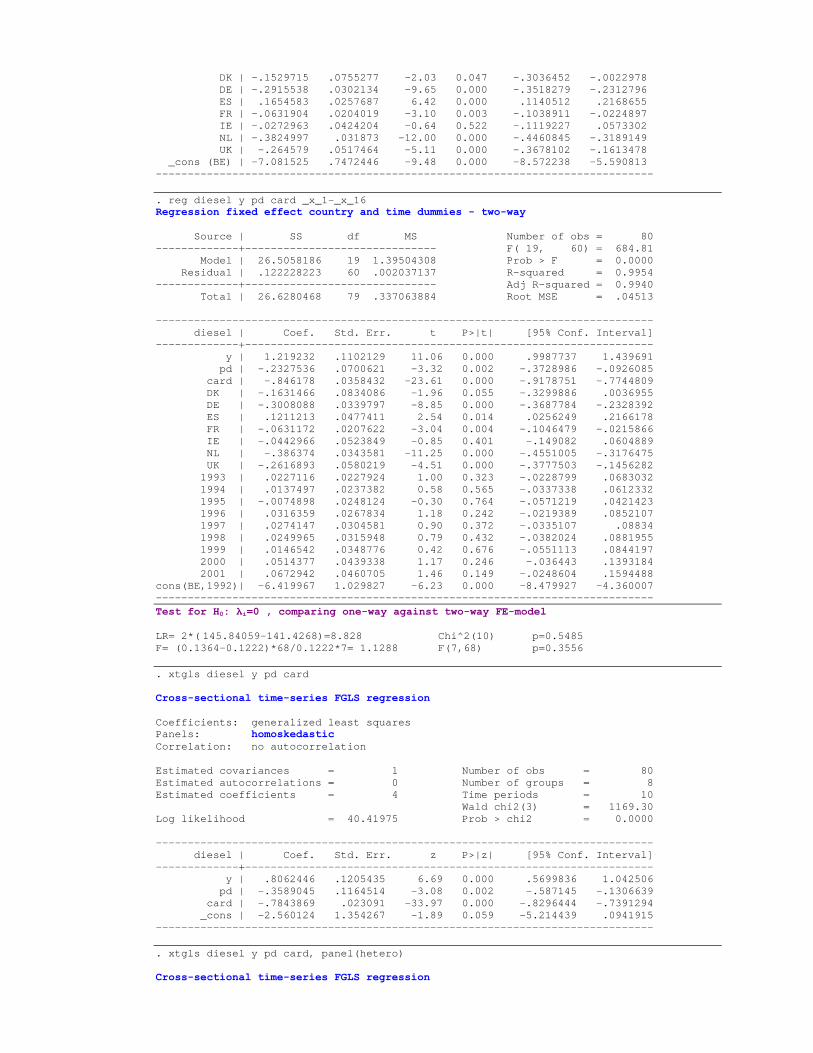
DK | -.1529715 .0755277 -2.03 0.047 -.3036452 -.0022978 DE | -.2915538 .0302134 -9.65 0.000 -.3518279 -.2312796 ES | .1654583 .0257687 6.42 0.000 .1140512 .2168655 FR | -.0631904 .0204019 -3.10 0.003 -.1038911 -.0224897 IE | -.0272963 .0424204 -0.64 0.522 -.1119227 .0573302 NL | -.3824997 .031873 -12.00 0.000 -.4460845 -.3189149 UK | -.264579 .0517464 -5.11 0.000 -.3678102 -.1613478 _cons (BE) | -7.081525 .7472446 -9.48 0.000 -8.572238 -5.590813 ------------------------------------------------------------------------------ . reg diesel y pd card _x_1-_x_16 Regression fixed effect country and time dummies - two-way Source | SS df MS Number of obs = 80 -------------+------------------------------ F( 19, 60) = 684.81 Model | 26.5058186 19 1.39504308 Prob > F = 0.0000 Residual | .122228223 60 .002037137 R-squared = 0.9954 -------------+------------------------------ Adj R-squared = 0.9940 Total | 26.6280468 79 .337063884 Root MSE = .04513 ------------------------------------------------------------------------------ diesel | Coef. Std. Err. t P>|t| [95% Conf. Interval] -------------+---------------------------------------------------------------- y | 1.219232 .1102129 11.06 0.000 .9987737 1.439691 pd | -.2327536 .0700621 -3.32 0.002 -.3728986 -.0926085 card | -.846178 .0358432 -23.61 0.000 -.9178751 -.7744809 DK | -.1631466 .0834086 -1.96 0.055 -.3299886 .0036955 DE | -.3008088 .0339797 -8.85 0.000 -.3687784 -.2328392 ES | .1211213 .0477411 2.54 0.014 .0256249 .2166178 FR | -.0631172 .0207622 -3.04 0.004 -.1046479 -.0215866 IE | -.0442966 .0523849 -0.85 0.401 -.149082 .0604889 NL | -.386374 .0343581 -11.25 0.000 -.4551005 -.3176475 UK | -.2616893 .0580219 -4.51 0.000 -.3777503 -.1456282 1993 | .0227116 .0227924 1.00 0.323 -.0228799 .0683032 1994 | .0137497 .0237382 0.58 0.565 -.0337338 .0612332 1995 | -.0074898 .0248124 -0.30 0.764 -.0571219 .0421423 1996 | .0316359 .0267834 1.18 0.242 -.0219389 .0852107 1997 | .0274147 .0304581 0.90 0.372 -.0335107 .08834 1998 | .0249965 .0315948 0.79 0.432 -.0382024 .0881955 1999 | .0146542 .0348776 0.42 0.676 -.0551113 .0844197 2000 | .0514377 .0439338 1.17 0.246 -.036443 .1393184 2001 | .0672942 .0460705 1.46 0.149 -.0248604 .1594488 cons(BE,1992)| -6.419967 1.029827 -6.23 0.000 -8.479927 -4.360007 ------------------------------------------------------------------------------ Test for H0: λi=0 , comparing one-way against two-way FE-model LR= 2*( 145.84059-141.4268)=8.828 Chi^2(10) p=0.5485 F= (0.1364-0.1222)*68/0.1222*7= 1.1288 F(7,68) p=0.3556 . xtgls diesel y pd card Cross-sectional time-series FGLS regression Coefficients: generalized least squares Panels: homoskedastic Correlation: no autocorrelation Estimated covariances = 1 Number of obs = 80 Estimated autocorrelations = 0 Number of groups = 8 Estimated coefficients = 4 Time periods = 10 Wald chi2(3) = 1169.30 Log likelihood = 40.41975 Prob > chi2 = 0.0000 ------------------------------------------------------------------------------ diesel | Coef. Std. Err. z P>|z| [95% Conf. Interval] -------------+---------------------------------------------------------------- y | .8062446 .1205435 6.69 0.000 .5699836 1.042506 pd | -.3589045 .1164514 -3.08 0.002 -.587145 -.1306639 card | -.7843869 .023091 -33.97 0.000 -.8296444 -.7391294 _cons | -2.560124 1.354267 -1.89 0.059 -5.214439 .0941915 ------------------------------------------------------------------------------ . xtgls diesel y pd card, panel(hetero) Cross-sectional time-series FGLS regression

Coefficients: generalized least squares Panels: heteroskedastic Correlation: no autocorrelation Estimated covariances = 8 Number of obs = 80 Estimated autocorrelations = 0 Number of groups = 8 Estimated coefficients = 4 Time periods = 10 Wald chi2(3) = 2307.26 Log likelihood = 56.26765 Prob > chi2 = 0.0000 ------------------------------------------------------------------------------ diesel | Coef. Std. Err. z P>|z| [95% Conf. Interval] -------------+---------------------------------------------------------------- y | 1.017673 .1083898 9.39 0.000 .805233 1.230113 pd | -.449832 .077441 -5.81 0.000 -.6016136 -.2980504 card | -.7666731 .0159832 -47.97 0.000 -.7979996 -.7353467 _cons | -4.857005 1.181773 -4.11 0.000 -7.173237 -2.540773 ------------------------------------------------------------------------------ . xtgls diesel y pd card, panel(correlated) Cross-sectional time-series FGLS regression Coefficients: generalized least squares Panels: heteroskedastic with cross-sectional correlation Correlation: no autocorrelation Estimated covariances = 36 Number of obs = 80 Estimated autocorrelations = 0 Number of groups = 8 Estimated coefficients = 4 Time periods = 10 Wald chi2(3) = 46506.78 Log likelihood = 148.8087 Prob > chi2 = 0.0000 ------------------------------------------------------------------------------ diesel | Coef. Std. Err. z P>|z| [95% Conf. Interval] -------------+---------------------------------------------------------------- y | .7833108 .0191966 40.80 0.000 .7456862 .8209355 pd | -.3321969 .0164491 -20.20 0.000 -.3644366 -.2999572 card | -.7859309 .0040034 -196.32 0.000 -.7937774 -.7780844 _cons | -2.262758 .2219776 -10.19 0.000 -2.697826 -1.82769 ------------------------------------------------------------------------------ . xtgls diesel y pd card, panel(correlated) corr(ar1) Cross-sectional time-series FGLS regression Coefficients: generalized least squares Panels: heteroskedastic with cross-sectional correlation Correlation: common AR(1) coefficient for all panels (0.9665) Estimated covariances = 36 Number of obs = 80 Estimated autocorrelations = 1 Number of groups = 8 Estimated coefficients = 4 Time periods = 10 Wald chi2(3) = 9790.46 Log likelihood = 182.1719 Prob > chi2 = 0.0000 ------------------------------------------------------------------------------ diesel | Coef. Std. Err. z P>|z| [95% Conf. Interval] -------------+---------------------------------------------------------------- y | 1.018488 .07707 13.22 0.000 .8674341 1.169543 pd | -.0711882 .0146844 -4.85 0.000 -.0999692 -.0424073 card | -.8074713 .0115425 -69.96 0.000 -.8300942 -.7848483 _cons | -3.968646 .8122939 -4.89 0.000 -5.560713 -2.376579 ------------------------------------------------------------------------------ . xtgls diesel y pd card, panel(correlated) corr(psar1) Cross-sectional time-series FGLS regression Coefficients: generalized least squares Panels: heteroskedastic with cross-sectional correlation Correlation: panel-specific AR(1) Estimated covariances = 36 Number of obs = 80 Estimated autocorrelations = 8 Number of groups = 8 Estimated coefficients = 4 Time periods = 10

Wald chi2(3) = 10410.18 Log likelihood = 147.9478 Prob > chi2 = 0.0000 ------------------------------------------------------------------------------ diesel | Coef. Std. Err. z P>|z| [95% Conf. Interval] -------------+---------------------------------------------------------------- y | 1.291594 .0555141 23.27 0.000 1.182788 1.4004 pd | -.096869 .0121108 -8.00 0.000 -.1206057 -.0731322 card | -.8507615 .0111222 -76.49 0.000 -.8725606 -.8289625 _cons | -7.087153 .5987569 -11.84 0.000 -8.260695 -5.913611 ------------------------------------------------------------------------------ . xtgls diesel y pd card, panel(hetero) corr(psar1) Cross-sectional time-series FGLS regression Coefficients: generalized least squares Panels: heteroskedastic Correlation: panel-specific AR(1) Estimated covariances = 8 Number of obs = 80 Estimated autocorrelations = 8 Number of groups = 8 Estimated coefficients = 4 Time periods = 10 Wald chi2(3) = 1234.34 Log likelihood = 161.242 Prob > chi2 = 0.0000 ------------------------------------------------------------------------------ diesel | Coef. Std. Err. z P>|z| [95% Conf. Interval] -------------+---------------------------------------------------------------- y | .9132192 .1250445 7.30 0.000 .6681365 1.158302 pd | -.0857943 .0347558 -2.47 0.014 -.1539143 -.0176743 card | -.8594665 .0276366 -31.10 0.000 -.9136332 -.8052998 _cons | -3.243283 1.329919 -2.44 0.015 -5.849876 -.6366894 ------------------------------------------------------------------------------ . xtgls diesel y pd card, corr(psar1) Cross-sectional time-series FGLS regression Coefficients: generalized least squares Panels: homoskedastic Correlation: panel-specific AR(1) Estimated covariances = 1 Number of obs = 80 Estimated autocorrelations = 8 Number of groups = 8 Estimated coefficients = 4 Time periods = 10 Wald chi2(3) = 336.76 Log likelihood = 138.1393 Prob > chi2 = 0.0000 ------------------------------------------------------------------------------ diesel | Coef. Std. Err. z P>|z| [95% Conf. Interval] -------------+---------------------------------------------------------------- y | 1.036291 .1498768 6.91 0.000 .7425376 1.330044 pd | -.0655656 .0589673 -1.11 0.266 -.1811395 .0500083 card | -.8724396 .0482841 -18.07 0.000 -.9670748 -.7778045 _cons | -4.451799 1.606996 -2.77 0.006 -7.601453 -1.302145 ------------------------------------------------------------------------------ . xtabond diesel y pd card Arellano-Bond dynamic panel-data estimation Number of obs = 64 Group variable (i): id Number of groups = 8 Wald chi2(4) = 637.15 Time variable (t): time Obs per group: min = 8 avg = 8 max = 8 One-step results ------------------------------------------------------------------------------ D.diesel | Coef. Std. Err. z P>|z| [95% Conf. Interval] -------------+---------------------------------------------------------------- diesel | LD | .2061316 .1190926 1.73 0.083 -.0272856 .4395488 y |

D1 | 1.070071 .1797725 5.95 0.000 .717723 1.422418 pd | D1 | -.1124007 .0642994 -1.75 0.080 -.2384252 .0136239 card | D1 | -.6650061 .1277177 -5.21 0.000 -.9153282 -.414684 _cons | -.000132 .0048327 -0.03 0.978 -.009604 .0093399 ------------------------------------------------------------------------------ Sargan test of over-identifying restrictions: chi2(35) = 42.38 Prob > chi2 = 0.1826 Arellano-Bond test that average autocovariance in residuals of order 1 is 0: H0: no autocorrelation z = -2.93 Pr > z = 0.0034 Arellano-Bond test that average autocovariance in residuals of order 2 is 0: H0: no autocorrelation z = 1.53 Pr > z = 0.1272 . xtabond diesel y pd card, lags(1) Arellano-Bond dynamic panel-data estimation Number of obs = 64 Group variable (i): id Number of groups = 8 Wald chi2(4) = 637.15 Time variable (t): time Obs per group: min = 8 avg = 8 max = 8 One-step results ------------------------------------------------------------------------------ D.diesel | Coef. Std. Err. z P>|z| [95% Conf. Interval] -------------+---------------------------------------------------------------- diesel | LD | .2061316 .1190926 1.73 0.083 -.0272856 .4395488 y | D1 | 1.070071 .1797725 5.95 0.000 .717723 1.422418 pd | D1 | -.1124007 .0642994 -1.75 0.080 -.2384252 .0136239 card | D1 | -.6650061 .1277177 -5.21 0.000 -.9153282 -.414684 _cons | -.000132 .0048327 -0.03 0.978 -.009604 .0093399 ------------------------------------------------------------------------------ Sargan test of over-identifying restrictions: chi2(35) = 42.38 Prob > chi2 = 0.1826 Arellano-Bond test that average autocovariance in residuals of order 1 is 0: H0: no autocorrelation z = -2.93 Pr > z = 0.0034 Arellano-Bond test that average autocovariance in residuals of order 2 is 0: H0: no autocorrelation z = 1.53 Pr > z = 0.1272 . xtabond diesel y pd card, lags(2) Arellano-Bond dynamic panel-data estimation Number of obs = 56 Group variable (i): id Number of groups = 8 Wald chi2(5) = 395.82 Time variable (t): time Obs per group: min = 7 avg = 7 max = 7 One-step results ------------------------------------------------------------------------------ D.diesel | Coef. Std. Err. z P>|z| [95% Conf. Interval] -------------+---------------------------------------------------------------- diesel | LD | .125125 .1552441 0.81 0.420 -.1791478 .4293978 L2D | -.0962694 .0933966 -1.03 0.303 -.2793234 .0867846 y | D1 | 1.216902 .2014503 6.04 0.000 .8220671 1.611738 pd | D1 | -.1347477 .0720007 -1.87 0.061 -.2758664 .0063711 card | D1 | -.8438203 .1327199 -6.36 0.000 -1.103946 -.5836941 _cons | .0047901 .0062476 0.77 0.443 -.007455 .0170352 ------------------------------------------------------------------------------ Sargan test of over-identifying restrictions: chi2(33) = 37.00 Prob > chi2 = 0.2896

Arellano-Bond test that average autocovariance in residuals of order 1 is 0: H0: no autocorrelation z = -3.49 Pr > z = 0.0005 Arellano-Bond test that average autocovariance in residuals of order 2 is 0: H0: no autocorrelation z = 2.30 Pr > z = 0.0217 . xtabond diesel y l(0/1).pd card, lags(2) Arellano-Bond dynamic panel-data estimation Number of obs = 56 Group variable (i): id Number of groups = 8 Wald chi2(6) = 373.07 Time variable (t): time Obs per group: min = 7 avg = 7 max = 7 One-step results ------------------------------------------------------------------------------ D.diesel | Coef. Std. Err. z P>|z| [95% Conf. Interval] -------------+---------------------------------------------------------------- diesel | LD | .1635903 .1668486 0.98 0.327 -.1634269 .4906075 L2D | -.0886154 .0957733 -0.93 0.355 -.2763276 .0990968 y | D1 | 1.173976 .2078943 5.65 0.000 .7665102 1.581441 pd | D1 | -.1503338 .0787279 -1.91 0.056 -.3046377 .0039701 LD | -.0120166 .0809957 -0.15 0.882 -.1707653 .146732 card | D1 | -.7752369 .1422169 -5.45 0.000 -1.053977 -.4964969 _cons | .0031297 .0066418 0.47 0.637 -.009888 .0161474 ------------------------------------------------------------------------------ Sargan test of over-identifying restrictions: chi2(33) = 42.19 Prob > chi2 = 0.1312 Arellano-Bond test that average autocovariance in residuals of order 1 is 0: H0: no autocorrelation z = -3.60 Pr > z = 0.0003 Arellano-Bond test that average autocovariance in residuals of order 2 is 0: H0: no autocorrelation z = 2.23 Pr > z = 0.0258 . xtabond diesel y l(0/1).pd card, lags(1) Arellano-Bond dynamic panel-data estimation Number of obs = 64 Group variable (i): id Number of groups = 8 Wald chi2(5) = 612.66 Time variable (t): time Obs per group: min = 8 avg = 8 max = 8 One-step results ------------------------------------------------------------------------------ D.diesel | Coef. Std. Err. z P>|z| [95% Conf. Interval] -------------+---------------------------------------------------------------- diesel | LD | .2376583 .1281778 1.85 0.064 -.0135656 .4888821 y | D1 | 1.063859 .1851579 5.75 0.000 .7009561 1.426762 pd | D1 | -.1343749 .0721187 -1.86 0.062 -.2757248 .0069751 LD | .0072949 .0722492 0.10 0.920 -.1343109 .1489006 card | D1 | -.623344 .13655 -4.56 0.000 -.8909772 -.3557109 _cons | -.0016841 .0052844 -0.32 0.750 -.0120414 .0086732 ------------------------------------------------------------------------------ Sargan test of over-identifying restrictions: chi2(35) = 42.17 Prob > chi2 = 0.1886 Arellano-Bond test that average autocovariance in residuals of order 1 is 0: H0: no autocorrelation z = -2.97 Pr > z = 0.0030 Arellano-Bond test that average autocovariance in residuals of order 2 is 0: H0: no autocorrelation z = 1.50 Pr > z = 0.1323 . xtabond diesel y l(0/2).pd card, lags(1)

Arellano-Bond dynamic panel-data estimation Number of obs = 56 Group variable (i): id Number of groups = 8 Wald chi2(6) = 431.77 Time variable (t): time Obs per group: min = 7 avg = 7 max = 7 One-step results ------------------------------------------------------------------------------ D.diesel | Coef. Std. Err. z P>|z| [95% Conf. Interval] -------------+---------------------------------------------------------------- diesel | LD | .0118841 .1346477 0.09 0.930 -.2520205 .2757886 y | D1 | 1.272778 .1854081 6.86 0.000 .909385 1.636172 pd | D1 | -.1554671 .0737939 -2.11 0.035 -.3001006 -.0108336 LD | .0132314 .0779292 0.17 0.865 -.1395071 .1659698 L2D | -.0870453 .0846661 -1.03 0.304 -.2529878 .0788973 card | D1 | -.8381178 .1384569 -6.05 0.000 -1.109488 -.5667473 _cons | .0036044 .0062872 0.57 0.566 -.0087182 .015927 ------------------------------------------------------------------------------ Sargan test of over-identifying restrictions: chi2(34) = 49.12 Prob > chi2 = 0.0451 Arellano-Bond test that average autocovariance in residuals of order 1 is 0: H0: no autocorrelation z = -2.41 Pr > z = 0.0160 Arellano-Bond test that average autocovariance in residuals of order 2 is 0: H0: no autocorrelation z = 1.22 Pr > z = 0.2209 . xtabond diesel l(0/1).(y pd card), lags(1) Arellano-Bond dynamic panel-data estimation Number of obs = 64 Group variable (i): id Number of groups = 8 Wald chi2(7) = 667.97 Time variable (t): time Obs per group: min = 8 avg = 8 max = 8 One-step results ------------------------------------------------------------------------------ D.diesel | Coef. Std. Err. z P>|z| [95% Conf. Interval] -------------+---------------------------------------------------------------- diesel | LD | .4025039 .1658613 2.43 0.015 .0774216 .7275861 y | D1 | .4540846 .3922962 1.16 0.247 -.3148019 1.222971 LD | .3990382 .3736737 1.07 0.286 -.3333488 1.131425 pd | D1 | -.153973 .075777 -2.03 0.042 -.3024931 -.0054529 LD | -.0489411 .0766681 -0.64 0.523 -.1992079 .1013256 card | D1 | -.9990571 .1652028 -6.05 0.000 -1.322849 -.6752655 LD | .4916564 .1668064 2.95 0.003 .1647219 .8185908 _cons | .0020583 .0057695 0.36 0.721 -.0092497 .0133663 ------------------------------------------------------------------------------ Sargan test of over-identifying restrictions: chi2(35) = 38.53 Prob > chi2 = 0.3130 Arellano-Bond test that average autocovariance in residuals of order 1 is 0: H0: no autocorrelation z = -3.63 Pr > z = 0.0003 Arellano-Bond test that average autocovariance in residuals of order 2 is 0: H0: no autocorrelation z = 1.89 Pr > z = 0.0586 ------------------------------------------------------------------------------------------