chapter five demand estimation -...

of 22

CHAPTER FIVE DEMAND ESTIMATION

Estimating demand for the firm’s product is an essential and continuing

process. After all, decisions to enter new market, decisions concerning

production, planning production capacity, and investment in fixed assets

inventory plans as well as pricing and investment strategies are all

depends on demand estimation.

The estimated demand function provides managers with an accurate

way to predict future demand for the firm’s product as well as set of

elasticities that allow managers to know in advance the consequences

of planned changes in prices, competitors’ prices, variations in

consumers’ income, or the expected changes in any of the other factors

affecting demand.

This chapter will provide you with a simplified version of the simple and

multiple regression analyses and techniques that belong to a field called

“Econometrics”, which focuses on the use of statistical techniques and

economic theories in dealing with economic problems.

Managers may not need to estimate demand by themselves, especially

in big firms. They may assign such technical tasks to their research

department or hire outsider consulting firms (outsourcing) to do the job.

However, a manager does need at least to have some basic knowledge

of econometrics, to be able to read and understand reports.

By the end of this chapter, you will be able to do simple demand

estimation, or at least to be able to read and understand the computer

printouts and reports presented to you.

In the following pages, we will study regression analysis and how it can

be used in demand estimation and how to find the coefficients of

demand equation. The question is how these coefficients are estimated,

or generally how demand is estimated.

of 22

Regression Analysis Regression analysis is a statistical technique for finding the best

relationship between dependent variable and selected independent

variable(s).

Dependent variable: depends on the value of other variables. It is the

primary interest to researchers.

Independent (explanatory) variable: used to explain the variation in

the dependent variable.

Regression analysis is commonly used by economists to estimate

demand for a good or service.

There are two types of statistical analysis:

1. Simple Regression Analysis: The use of one independent variable

Y = a + bX +µ

Where:

Y: dependent variable, amount to be determined

a: constant value; y-intercept

b: slope (regression coefficients), or parameters to be estimated (it

measures the impact of independent variable)

X: independent (or explanatory) variable, used to explain the variation in

the dependent variable

µ: random error

2. Multiple Regression Analysis: The use of more than one independent variable

Y = a + b1X1 + b2X2 + ….+ bkXk + µ

(k= number of independent variable in the regression model)

The well-known method of ordinary least squares (OLS) is used in our

regression analysis. Some of the assumptions of OLS include.

1. Independent (explanatory) variables are independent from the

dependent variable and independent from each other.

of 22

2. The error terms (µ) are independent and identically distributed

normal random variables, with mean equal to zero.

How regression analysis is done? There are certain steps to conduct reg. analysis.

1. Identify the relevant variables

2. Obtain data on the variables

3. Specify the regression model

4. Estimate the parameters (coefficients)

5. Interpret the results

6. Statistical evaluation of the results (testing statistical significance of

model)

7. Use the results in decision making (forecasting using reg. results).

1. Identification of variables and data collection: Here, we try to answer the question of what variables to be included in

regression analysis; what variables are important

The role of economic theory, the availability of data and other

constraints help in determining which variables to be included

The role of economic theory:

o In estimating the demand for a particular good or service, we have

to determine all the factors that might influence this demand.

o Economic theory helps by considering the right set of variables to

be considered when estimating demand for the good. It also helps

in determining the relationship between Qd and these variables;

e.g.; we expect a negative sign for the coefficient of P because of

the negative relation between P and Qd. if the good under

consideration is a normal good, we expect a positive sign the for

the coefficient of income because of the positive relationship

between income and the demand for normal good, etc…

of 22

In reality, however, the availability of data and the cost of generating new data may determine what to include.

o Some variables are easy to find and to measure and quantify, like

prices, number of consumers and may be income …

o Sometimes it is difficult to get data for the original variables use

proxy

o Some variables are hard to quantify such as location (urban,

suburban, rural) or tastes and preferences (like, dislike, indifferent,

…) ⇒ use dummy (binary) variables (1 if the event occurs and

zero otherwise. E.g., urban, 0 otherwise) or (1 if like, 0 otherwise).

o The main types of data used in regression are:

1. Cross sectional: provide information about the variables

for a given time period (different individuals, goods, firms,

countries …)

2. Time series: give information about variables over a

number of periods of time (years, months, daily,…)

3. Pooled (Panel): Combinations of cross section and time

series data

o Data for studies pertaining to countries, regions, or industries are

readily available and reliable.

o Data for analysis of specific product categories may be more

difficult to obtain. The solution is to buy the data from data

providers, perform a consumer survey, focus groups, etc.

2. Specification of the model: This is where the relation between the dependent variable (say, Qd) and

the factors affecting it (the independent or explanatory variables) are

expressed in regression equation.

The estimation of regression equation involves searching for the best

linear relationship between variables.

of 22

The commonly used specification is to express the regression equation

in the additive liner function.

If equation is non-liner such as Multiplicative such as Q = APbYc,

transform nonlinear into linear using logarithm

It is double log (log is the natural log, also written as ln)

Log Q = a + bLog P + cLog Y

For the purpose of illustration, let us assume that we have obtained

cross-sectional data on college students of 30 randomly selected

college campuses during a particular month, with the following equation.

Qd = a + b1P + b2T - b3Pc + b4L + µ

Where:

Qd: Quantity demanded of pizza (average number of slices per capita

per month)

P: Average price of slice of pizza (in cents)

T: Annual tuition as proxy for income (in thousands of $s)

Pc: Price of cans of soft drinks (in cents)

L: Location of campuses (1 if urban area, 0 otherwise)

a: Constant value or Y intercept

bi: Coefficient of independent variables to be estimated (slope)

µ: Random error term standing for all other omitted variables.

The effect of each variable (the marginal impact) is the coefficient of that

variable in the regression equation. The impact of P is b1 (dQ/dP), the

impact of T is b2 (dQ/dT), etc…..

The elasticity of each variable is calculated as usual:

o QPb

QP

dPdQE 1d ×=×=

o QTb

QT

dTdQE 2T ×=×=

o QP

bQP

dPdQE c

3c

cPc ×=×=

o QLb

QL

dLdQE 4L ×=×=

of 22

3. Estimation of the regression coefficients: Given this particular set up of regression equation we can now estimate

the values of coefficients of the independent variable as well as the

intercept term. Using ordinary least squares (OLS) method

Usually statistical and econometrics packages are used to estimate

regression equation using excel and many other statistical packages

such as SPSS, SAS, EViews, LimDep, TSP…

Results are usually reported in regression equation or table format,

containing certain information such

Qd = 26.67 – 0.088P + 0.138T – 0.076Pc – 0.544L

(0.018) (0.0087) (0.020) (0.884)

R2 = 0.717 (The coefficient of determination)

67.0R2= (Adjusted R2

SE of Q estimate (SEE) = 1.64

F = 15.8 (F-Statistics)

Standard errors of the coefficient are listed in parentheses.

4. Interpretation of the regression coefficients: Analyzing regression results involves the following steps

o Checking the signs and magnitudes

o Computing elasticity coefficients

o Determining statistical significance

It also involves two tasks:

o Interpretation of coefficients

o Statistical evaluation of coefficients

What are the expected magnitude and signs of the estimated

coefficient?

Check signs of the coefficient according to economic theory and see if

they are as expected:

P: when price increases, Qd for Pizza decreases (negative sign)

of 22

T: Sign for proxy of income depends on whether pizza is a normal or

inferior good. (+,-)

Pc: expected sign for Pc is (-) because of complementary relation (Pc

increases, demand for pizza decreases)

L: Expected sign is (-) because in urban areas students have varieties

of restaurants (more substitutes), ⇒ they will consume less pizza

than their counterparts in other areas will.

Check the effect of each independent variable on the dependent

variable according to economic theory.

With regard to magnitude, we can see that each estimated coefficient

tells us how much the demand for pizza will change relative to a unit

change in each of the independent variables.

b1: a unit change in P changes Qd by 0.088 units in the opposite

direction.

b2: for a $1000 change in tuition, demand changes by 0.138 units.

b3: for a unit change in Pc, demand changes by 0.076 in opposite

direction

b4: students in urban areas will buy about half (0.544) less than those in

other areas.

Magnitude of regression coefficients is measured by elasticity of each

variable.

If P=100 (cents), T=14($000), Pc=110 (cents), L= 1

Qd = 26.67 – 0.088(100) + 0.138(14) – 0.076(110) – 0.544(1) = 10.898

807.0898.10

100088.0Ed −=×−= is somewhat inelastic

177.0898.10

14138.0ET =×= no great impact

767.0898.10

110076.0 −=×−=cpE is inelastic

05.0898.101544.0EL −=×−= dose not really matter

of 22

5. Statistical evaluation of the regression results Regression results are based on a sample.

How confident are we that these results are truly reflective of

population?

The basic test of the statistical significance using each of the estimated

regression coefficients is done separately using t-test.

t- Test

t-test is conducted by computing t-value or t-statistic for each of the

estimated coefficient, to test the impact of each variable separately.

t = (estimated coefficient – population value of the coefficient) / standard

error of the coefficient

ib

ii

Sbbt −

=

bi is assumed equal to zero in the null hypothesis ⇒ ib

i

Sbt =

We usually compare the estimated (observed) t-value (ib

i

Sbt = ) to the

critical value from t-table, t α, n-k-1

where:

α = level of significance (it is an error rate of unusual samples with their

false inference from a sample to a population)

n = number of observations,

k = number of independent/ explanatory variables.

n-k-1 = degrees of freedom: the number of free or linearly independent

sample observations used in the calculation of statistic.

To compare estimated t-value to critical t-value.

of 22

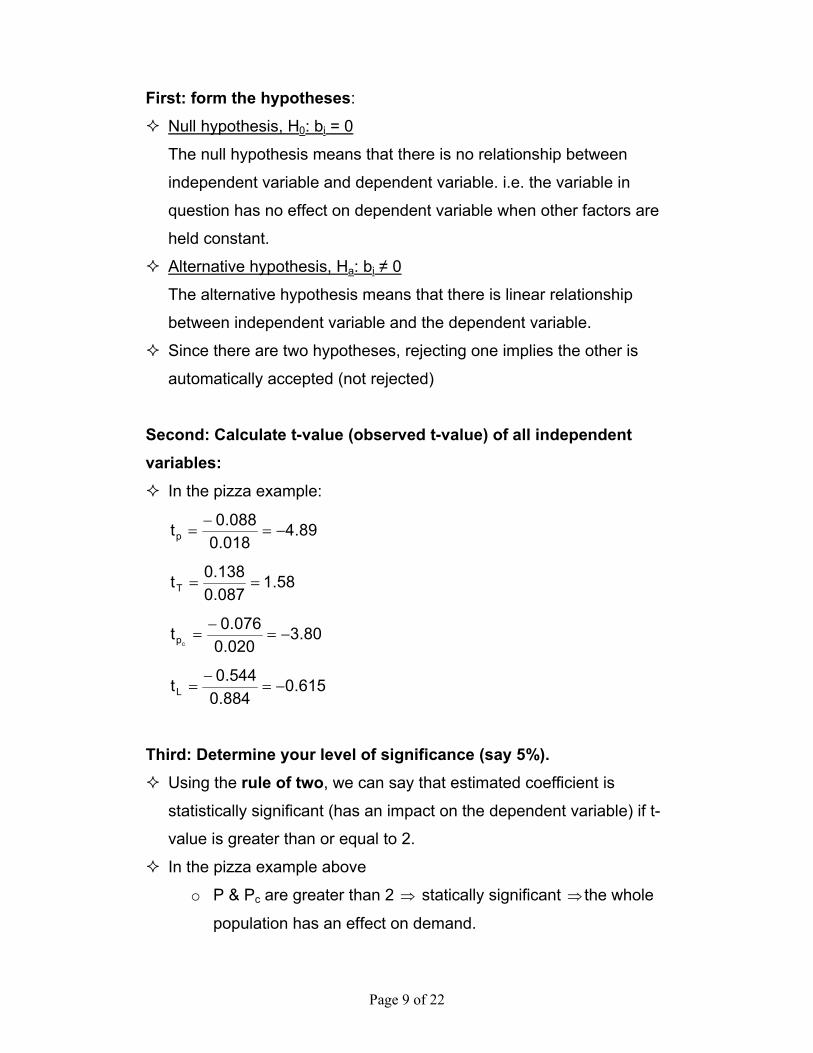
First: form the hypotheses:

Null hypothesis, H0: bi = 0

The null hypothesis means that there is no relationship between

independent variable and dependent variable. i.e. the variable in

question has no effect on dependent variable when other factors are

held constant.

Alternative hypothesis, Ha: bi ≠ 0

The alternative hypothesis means that there is linear relationship

between independent variable and the dependent variable.

Since there are two hypotheses, rejecting one implies the other is

automatically accepted (not rejected)

Second: Calculate t-value (observed t-value) of all independent variables:

In the pizza example:

89.4018.0088.0tp −=

−=

58.1087.0138.0tT ==

80.3020.0076.0t

cp −=−

=

615.0884.0544.0tL −=

−=

Third: Determine your level of significance (say 5%). Using the rule of two, we can say that estimated coefficient is

statistically significant (has an impact on the dependent variable) if t-

value is greater than or equal to 2.

In the pizza example above

o P & Pc are greater than 2 ⇒ statically significant ⇒ the whole

population has an effect on demand.

of 22

o T& L are Less than 2 ⇒ statistically insignificant ⇒ the population

as no effect on demand.

α = 0.05, n = 30, k= 4

t α, n-k-1 = t 0.05, 30-4-1 = t 05, 25 = 2.060

Fourth: Conclusion

Compare absolute t-value with the critical t-value:

If absolute t-value > critical t-value, reject H0 and conclude that

estimated coefficient is statistically significant, otherwise accept H0.

var. t-value critical Decision Conclusion P 4.889 > 2.060 reject significant

T 1.683 < 2.060 don’t reject not significant

Pc 3.800 > 2.060 reject significant

L 0.615 < 2.060 do not reject not significant

Significant means there is linear relationship between the independent

and dependent variables. The independent variable has a true impact

on the dependent variable or it is important in explaining variation in the

dependent variable (Qd in our example),

Not significant means there is no linear relationship between the

independent and dependent variables

-2.060 2.060

Reject H0 Accept H0

0

Reject H0

of 22

Testing the performance of the Regression Model – R2 The overall results are tested using the coefficient of determinations, R2.

R2 is to evaluate the deterministic power of the regression model.

R2 is used to test whether the regression model is good, i.e., to test the

goodness of fit of the regression line to actual data.

R2 measures the percentage of total variation in the dependent variable

that is explained by the variation in all of the independent variables in

the regression model.

TSSESS1

TSSRSSR2 −==

Where,

TSS: total sum of squares; it is the sum of squared total variation in the

dependent variables around its mean (explained & unexplained)

RSS: regression sum of square (explained variation)

ESS: Error of square (unexplained variation)

0 < R2 < 1

R2 = 0 ⇒ variation in the dependent variable cannot be explained at all

by the variation in the independent variable.

R2 = 1 ⇒ all of the variation in the dependent variable can be explained

by the independent variables For statistical analysis, the closer R2 is to one, the better the regression

equation; i.e., the greater the explanatory power of the regression

equation.

Low value of R2 indicates the absence of some important variables from

the model.

In our example, R2 = 0.717. This means that about 72% of the variation

in the demand for pizza by college students can be explained by the

variation in the independent variables.

The value of R2 is affected by:

o The value of independent variables: the way R2 is calculated

causes its value to increase as more independent variables are

of 22

added to the regression model even if these variables do not have

any effect on the dependent variable.

o Types of data used: other factors held constant, time series data

generally produce a higher R2 than cross-sectional data. This is

because of series data has built-in trend over time to keep

dependent and independent variables moving closely together. A

good example of this is a time-series analysis of aggregate

consumption regressed on aggregate disposable income.

Regression analysis of this consumption function commonly

produces R2 of .95 and above.

Adjusted R2, 2R (The adjusted coefficient of determination),

As more and more variables are added, R2 usually increases.

Therefore, we use 2R to account for this “inflation" in R2 so that

equation with different numbers of independent variables can be more

fairly compared

In our example, 2R = 0.67 which indicates that about 67% of the

variation in Qd of pizza is explained by the variations in the independent

variables while 33% of these variations are unexplained by the model.

2R is calculated as

( )222 R11kn

kRR −−−

−=

( ) 67.072.0125472.0R 2 =−−=

of 22

F- test F-test is used to test the impact of overall explanatory power of the

whole model, or the joint effect of all explanatory variables as a group.

(i.e., testing the overall performance of the regression coefficients)

F-test measures the statistical significance of the entire regression

equation rather than of each individual coefficient as the t-test is

designed to do.

If it is used in simple regression (i.e., for a regression equation with only

one independent variable), then in effect it provides the same test as the

t-test for this particular variable.

The F-test is much more useful when two or more independent variables

are used.

It can then test whether all of these variables taken together are

statistically significant from zero, leaving the t-test to determine whether

each variable taken separately is statistically significant.

As in the t-test, we have to set our hypotheses.

First: form the hypotheses:

H0: All bi = 0 ( b1= b2 = b3 =…= bk = 0) (k= number of independent variable in the regression model)

There is no relation between the dependent variable and independent

variables. The model cannot explain any of the variation in the

dependent variable

Ha: at least one bi ≠ 0 A linear relation exists between dependent variable and at least one of

the independent variables.

of 22

Second: Calculate F-value F = (explained variation/k) / (unexplained variation/n-k-1)

( )

( ) 1kn/ESSk/RSS

1kn/YY

k/YYF 2

2

−−=

−−−

−=∑∑

RSS: regression some of squares

ESS: error sum of squares

n: number of observation

k: number of explanatory variables

But F maybe re-written in term of R2 as follows

( ) 1kn/R1k/RF 2

2

−−−=

In our example: F=15.8

The greater the value of F-statistics, the more confident the researcher

would be that variables included in the model have together a significant

effect on the dependent variable, and the model has a high explanatory

power.

Thus, the F test examines the significance of R2

Third: Determine your level of significance (say 5%) F α, k, n-k-1

α: level of significance

k: number of independent variables

n: number of observations or sample size

k, n-k-1: degrees of freedom

in our example: F.05, 4, 30-4-1 = F.05, 4, 25 = 2.76

Fourth: Compare F-value (observed F) with critical F-value If F > Critical F value reject H0 and conclude that a linear relation

exists between the dependent variable and at least one of the

independent variable

of 22

F= 15.8 > F.05, 4, 25 = 2.76

Reject H0, there is a linear relationship between the dependent variable

and at least one of the independent variables. The entire regression

model accounts for a statistically significant proportion of the variation in

the demand for pizza.

6. Forecasting:

Future values of demand can easily be predicted or forecasted by

plugging values of independent variables in the demand equation.

Only we have to be confident at a given level that the true Y is close to

the estimated Y.

Since we do not know the true Y, we can only say that it lies between a

given confidence interval.

The interval is Ŷ+ t α, n-k-1 X SEE

Confidence interval tells that we are, say, 95% confident that the

predicted value of Qd lies approximately between the two limits.

Implications of Regression Analysis for Decision Making Regression analysis can show which are the important factors, judging

from whether the variable is significant or not (what variables passed the

t-test and what did not pass.)

The magnitude and the level of coefficient indicate the importance of the

variables.

Computing elasticity will help in determining what may happen to total

revenue.

of 22

Correlation A measure of association is the correlation coefficient, r.

Correlation coefficient, r, indicates the strength and direction of a

linear relationship between two random variables

The correlation is defined only if both of the standard deviations are

finite and both of them are nonzero

If r = 0 the variables are independent

If r = 1, the correlation is perfect and positive. This is the case of an

increasing linear relationship

If r = -1, the correlation is perfect and negative. This is the case of an

decreasing linear relationship

If the value is in between, it indicates the degree of linear dependence

between the variables

The closer the coefficient is to either -1 or 1, the stronger the correlation

between the variable

The correlation coefficient is defined in terms of the covariance:

ZX

XZ

)zvar()Xvar()Z,Xcov()Z,X(corr

σσσ

==

–1 ≤ corr(X,Z) ≤ 1

corr(X,Z) = 1 mean perfect positive linear association

corr(X,Z) = –1 means perfect negative linear association

corr(X,Z) = 0 means no linear association

Association and Causation Regressions indicate association, but beware of jumping to the

conclusion of causation

Suppose you collect data on the number of swimmers at a beach and

the temperature and find:

Temperature = 61 + .04 Swimmers,

and R2 = .88.

of 22

o Surely the temperature and the number of swimmers is positively

related, but we do not believe that more swimmers caused the

temperature to rise.

o Furthermore, there may be other factors that determine the

relationship, for example the presence of rain, or whether or not it

is a weekend or weekday.

Education may lead to more income, and also more income may lead to

more education. The direction of causation is often unclear. But the

association is very strong.

of 22

Regression Problems

Identification Problem:

The identification problem refers to the difficulty of clearly identifying the

demand equation because of the effects of both supply and demand that

are often reflected in data used in the analysis.

The estimation of demand may produce biased results due to

simultaneous shifting of supply and demand curves.

Advanced estimation techniques, such as two-stage least squares and

indirect least squares, are used to correct this problem.

Multicollinearity

Two or more independent variables are highly correlated, thus it is

difficult to separate the effect each has on the dependent variable.

Passing the F-test as a whole, but failing the t-test for each coefficient is

a sign that multicollinearity exists.

A standard remedy is to drop one of the closely related independent

variables from the regression

Autocorrelation

Also known as serial correlation, occurs when the dependent variable

relates to the independent variable according to a certain pattern.

Possible causes:

o Effects on dependent variable exist that are not accounted for by the

independent variables.

o The relationship may be non-linear

The Durbin-Watson (DW) statistic is used to identify the presence of

autocorrelation.

To correct autocorrelation consider:

o Transforming the data into a different order of magnitude

o Introducing leading or lagging data

of 22

APPENDIX

Using MS-Excel in Regression: 1. Open a new file in Excel program and name it example-1.

2. Label the first column on your file Q, the second P. Insert the following

data collected by the research team in 1999.

Observations 1 2 3 4 5 6 7 8 9 10

Meals 180 590 430 250 275 720 660 490 700 210

Price 475 400 450 550 575 375 375 450 400 500

Observations 11 12 13 14 15 16 17 18 19 20

Meals 150 120 500 150 600 220 200 280 160 300

Price 480 650 300 330 350 660 650 540 720 600

3. Open Tools in the menu bar, choose Data Analysis and move to number

4 bellow. If Data Analysis does not appear on the Tools menu, click

“Add-Ins….”. on the Tools menu. In the Add-Ins window, choose

“Analysis ToolPack” and press OK.

of 22

4. Now, open tools once again and click the new title “Data Analysis”, and click Regression in the Data Analysis window, then OK.

5. In the regression dialog box, For “Input Y range”, select the Q column

of your data including the label cell. Move the cursor to “Input X range”,

select the P column from your data. Check the square beside “labels”. 6. Click “Output Range”, and click a cell bellow your data where you like

printing of the results to start.

of 22

7. Click OK. The results print out will look exactly as follows:

SUMMARY OUTPUT

Regression Statistics

Multiple R 0.66119647

R Square 0.43718077

Adjusted R Square 0.40591304

Standard Error 158.38729

Observations 20

ANOVA

df SS MS F Significance F

Regression 1 350756.1452 350756.113.98184982 0.001501539

Residual 18 451557.6048 25086.53

Total 19 802313.75

of 22

CoefficientsStandard Errort Stat P-value

Intercept 903.598862 149.8239232 6.0310721.05758E-05

P -1.1075257 0.296190743 -3.73923 0.001501539

Excel Exercise

1. Use the data in your text page 169 to confirm the results presented in

the text

2. The following table contains data on the number of apartments rented

(Q), the rental price (P) in BDs, the amount spent on advertisement (AD)

in hundreds of BDs, and the distance between the apartments and the

university (Dis) in miles.

Q 28 69 43 32 42 72 66 49 70 60 P 250 400 450 550 575 375 375 450 400 375 AD 11 24 15 31 34 22 12 24 22 10 Dis 12 6 5 7 4 2 5 7 4 5

a. Use Excel program to regress Q on the three explanatory variables.

b. Write the estimated demand equation for apartments.

chapter five demand estimation -...

Documents