estimation from indirect supervision with linear moments · estimation from indirect supervision...

Estimation from Indirect Supervision with Linear Moments

Aditi Raghunathan [email protected] Frostig [email protected] Duchi [email protected] Liang [email protected]

Stanford University, Stanford, CA

AbstractIn structured prediction problems where we haveindirect supervision of the output, maximummarginal likelihood faces two computational ob-stacles: non-convexity of the objective and in-tractability of even a single gradient computa-tion. In this paper, we bypass both obstacles for aclass of what we call linear indirectly-supervisedproblems. Our approach is simple: we solve alinear system to estimate sufficient statistics ofthe model, which we then use to estimate param-eters via convex optimization. We analyze thestatistical properties of our approach and showempirically that it is effective in two settings:learning with local privacy constraints and learn-ing from low-cost count-based annotations.1

1. IntroductionConsider the problem of estimating a probabilistic graph-ical model from indirect supervision, where only a partialview of the variables is available. We are interested in indi-rect supervision for two reasons: first, one might not trusta data collector and wish to use privacy mechanisms to re-veal only partial information about sensitive data (Warner,1965; Evfimievski et al., 2004; Dwork et al., 2006; Duchiet al., 2013). Second, if data is generated by human anno-tators, say in a crowdsourcing setting, it can often be morecost-effective to solicit lightweight annotations (Oded &Tomas, 1998; Mann & McCallum, 2008; Quadrianto et al.,2008; Liang et al., 2009). In both cases, we trade statisticalefficiency for another resource: privacy or annotator cost.

Indirect supervision is naturally handled by defining alatent-variable model where the structure of interest istreated as a latent variable. While statistically sensible,

1 This is an extended and updated version of our paper inProceedings of the 33 rd International Conference on MachineLearning, New York, NY, USA, 2016. JMLR: W&CP volume48. Copyright 2016 by the author(s).

learning latent-variable models poses two computationalchallenges. First, maximum marginal likelihood requiresnon-convex optimization, where popular procedures suchas gradient descent or Expectation Maximization (EM)(Dempster et al., 1977) are only guaranteed to converge tolocal optima. Second, even the computation of the gradientor performing the E-step can be intractable, requiring prob-abilistic inference on a loopy graphical model induced bythe indirect supervision (Chang et al., 2007; Graca et al.,2008; Liang et al., 2009).

In this paper, we propose an approach that bypasses bothcomputational obstacles for a class which we call linearindirectly-supervised learning problems. We lean on themethod of moments (Pearson, 1894), which has recentlyled to advances in learning latent-variable models (Hsuet al., 2009; Anandkumar et al., 2013; Chaganty & Liang,2014), although we do not appeal to tensor factorization.Instead, we express indirect supervision as a linear com-bination of the sufficient statistics of the model, which werecover by solving a simple noisy linear system. Once wehave the sufficient statistics, we use convex optimization tosolve for the model parameters. The key is that while su-pervision per example is indirect and leads to intractability,aggregation over a large number of examples renders theproblem tractable.

While our moments-based estimator yields computationalbenefits, we suffer some statistical loss relative to maxi-mum marginal likelihood. In Section 5, we compare theasymptotic variance of marginal-likelihood and moment-based estimators, and provide some geometric insight intotheir differences in Section 6. Finally, in Section 7, we ap-ply our framework empirically to our two motivating set-tings: (i) learning a regression model under local privacyconstraints, and (ii) learning a part-of-speech tagger withlightweight annotations. In both applications, we show thatour moments-based estimator obtains good accuracies.

arX

iv:1

608.

0310

0v1

[st

at.M

L]

10

Aug

201

6


x y omodel

pθ(y | x)

supervision

S(o | y)

Figure 1. We solve a structured prediction problem from x to y.During training, we observe not y, but indirect supervision o.

2. SetupNotation. We use superscripts to enumerate instances ina data sample (e.g. x(1), . . . , x(n)), and square-bracket in-dexing to enumerate components of a vector or sequence:x[b] denotes the component(s) of x associated with b. Fora real vector x ∈ Rd, we let x⊗2 def

= xx>.

Model. Consider the structured prediction task of map-ping an input x ∈ X to some output y ∈ Y . We model thismapping using a conditional exponential family

pθ(y | x) = expφ(x, y)>θ −A(θ;x), (1)

where φ : X × Y → Rd is the feature mapping,θ ∈ Rd is the parameter vector, and A(θ;x) =log∑y∈Y expφ(x, y)>θ is the log-partition function.

For concreteness, we specialize to conditional randomfields (CRFs) (Lafferty et al., 2001) over collections ofK-variate labels, where x = (x[1], . . . , x[L]) and y =(y[1], . . . , y[L]) ∈ [K]L; here L is the number of vari-ables and K is the number of possible labels per vari-able. We let C ⊆ 2[L] be the set of cliques in the CRF,so that the features decompose into a sum over cliques:φ(x, y) =

∑c∈C φc(y[c], x, c). As one particular exam-

ple, if C consists of all nodes 1, . . . , L and edgesbetween adjacent nodes 1, 2, . . . , L−1, L, the CRFis chain-structured.

Learning from indirect supervision. In the indirectlysupervised setting that is the focus of this paper, we do nothave access to y but rather only observations o ∈ O, whereo is drawn from a known supervision distribution S(o | y).

For each i = 1, . . . , n, let (x(i), y(i)) be drawn from someunknown data-generating distribution p∗ (by default, we donot assume the CRF is well-specified), and o(i) is drawnaccording to S(· | y(i)) as in Figure 1. The learning prob-lem is then the natural one: given the training examples(x(1), o(1)), . . . , (x(n), o(n)), we wish to produce an esti-mate θ for the model (1).

Maximum marginal likelihood. The classic paradigm isto maximize the marginal likelihood:

θmargdef= argmax

θE

log∑y∈Y

S(o | y)pθ(y | x)

, (2)

(x(i), o(i)) µ θlinear system convex optimization

Figure 2. Our approach is to (i) solve a linear system based onthe data (x(i), o(i)) to estimate the sufficient statistics µ, then(ii) use convex optimization to estimate the model parameters θ.

where E denotes an expectation over the training sample.While θmarg is often statistically efficient, there are twocomputational difficulties associated with this approach:

1. The log-likelihood objective (2) is typically non-convex, so computing θmarg exactly is in general in-tractable; see Section 6 for a more detailed discus-sion. Local algorithms like Expectation Maximization(Dempster et al., 1977) are only guaranteed to con-verge to local optima.

2. Computing the gradient or the E-step requires com-puting p(y | x, o) ∝ pθ(y | x)S(o | y), which isintractable, not due to the model pθ, but to the supervi-sion S. This motivates a number of relaxations (Gracaet al., 2008; Liang et al., 2009; Steinhardt & Liang,2015), but there are no guarantees on approximationquality.

Our approach: moment-based estimation. We presenta simple approach to circumvent the above issues for arestricted class of models, in the same vein as Chaganty& Liang (2014). To begin, consider the fully-supervisedsetting, where we observe examples (x(i), y(i)). Inthis case, we could maximize the likelihood E[log pθ(y |x)], solving argmaxθµ>θ − E[A(θ;x)], where µ def

=

E[φ(x, y)] ∈ Rd are the sufficient statistics, which con-verge to µ∗ def

= E[φ(x, y)]. Therefore, if we could constructa consistent estimate µ of µ∗, then we could solve the sameconvex optimization problem used in the fully-supervisedestimator.

Of course, we do not have access to E[φ(x, y)]. Instead,in our (linearly) indirectly supervised setting, we are ableto define an observation function β(x, o) ∈ Rd which isnonetheless in expectation equal to the population suffi-cient statistics:

E[β(x, o) | x] = φ(x, y), E[β(x, o)] = µ∗. (3)

In general, we construct β(x, o) by solving a linear system.Putting the pieces together yields our estimator (Figure 2):

1. Sufficient statistics: µ = E[β(x, o)].

2. Parameters: θmomdef= arg maxθµ− E[A(θ;x)].

In the next two sections, we describe the observation func-tion β(x, o) for learning with local privacy (Section 3) andlightweight annotations (Section 4).


3. Learning under local privacySuppose we wish to estimate a conditional distributionpθ(y | x), where x is non-sensitive information about anindividual and y contains sensitive information (for ex-ample, income or disease status). Individuals, becauseof a variety of reasons—mistrust, embarrassment, fear ofdiscrimination—may wish to keep y private and insteadrelease some o ∼ S(· | y). To quantify the amount ofprivacy afforded by S, we turn to the literature on pri-vacy in databases and theoretical computer science (Ev-fimievski et al., 2004; Dwork et al., 2006) and say that Sis α-differentially private if any two y, y′ have comparableprobability (up to a factor of exp(α)) of generating o:

supo,y,y′

S(o | y)

S(o | y′)≤ exp(α). (4)

What S should we employ? We first explore the classicalrandomized response (RR) mechanism (Section 3.1), andthen develop a new mechanism that leverages the graphicalmodel structure (Section 3.2).

3.1. Classic randomized response

Warner (1965) proposed the now-classical randomized re-sponse technique, which proceeds as follows: For somefixed (generally small) ε > 0, the respondent reveals y withprobability ε and with probability 1 − ε draws a samplefrom a (known) base distribution u—generally uniform—over Y . Formally, the classical randomized response super-vision is

S(o | y)def= εI[o = y] + (1− ε)u(o). (5)

Estimation. Our goal is to construct a function β satis-fying (3). Towards that end, let us start with what we canestimate and expand based on (5):

E[φ(x, o)] = εE[φ(x, y)] + (1− ε)E[φ(x, y′)], (6)

where y′ ∼ u. Rearranging (6), we see that we can solvefor µ∗ = E[φ(x, y)]. Indeed, if we define the observationfunction:

β(x, o)def=

φ(x, o)− (1− ε)E[φ(x, y′) | x]

ε, (7)

we can verify that E[β(x, o)] = µ∗.

Privacy. We can check that the ratio S(o | y)/S(o |y′) ≤ 1 + ε+(1−ε)u(o)

(1−ε)u(o) , so classical randomized responseis ε

(1−ε) mino u(o) -differentially private. For any distributionu, this value is at least ε

1−ε |Y|, a linear dependence on |Y|.In classical randomized response settings, |Y| = 2, whichis unproblematic. In contrast, in structured prediction set-tings, the number of labels is exponential in the number of

variables (|Y| = KL), so we must take ε = O(α|Y|

). The

asymptotic variance of θmom scales as ε−2 (as will be shownin Section 5), which makes classical randomized responseunusable for structured prediction.

3.2. Structured randomized response

With this difficulty in mind, we recognize that we mustsomehow leverage the structure of the sufficient statisticsvector φ(x, y) to perform estimation. In particular, weshow that the supervision should only depend on the suf-ficient statistics:

Proposition 1. Let O be the set in which observationslive. For any privacy mechanism S(o | x, y) that is α-differentially private, there exists a mechanism S′(o′ |φ(x, y)) that is at least α-differentially private, and for anyset A ⊆ O, we have

P[o′ ∈ A | x] = P[o ∈ A | x], (8)

where o′ ∼ S′(· | φ(x, y)) and o ∼ S(· | x, y).

In short, we can always construct S′ that only uses the suffi-cient statistics φ(x, y) but yields the same joint distributionover the pairs (x, o). Furthermore, S′ is at least as pri-vate as the original mechanism S. See Appendix A.1 for aproof.

This motivates a focus exclusively on mechanisms that usesufficient statistics, and in particular, we consider the fol-lowing two structured randomized response mechanisms.Our schemes are both two-phase procedures that first bi-narize the sufficient statistics, and then release a set of ob-servations inspired by Duchi et al.’s minimax optimal ap-proach to estimating a multinomial distribution. For t > 0,let qt

def= et/2

1+et/2. Assume each coordinate of the statistics

φ lies in the interval [0, c] for some positive scalar c. Fori ∈ 1, . . . , d, draw o[i] as a Bernoulli variable with bias1cφ(x, y)[i]. Then:

(Coordinate release) Draw a coordinate j ∈ 1, . . . , dfrom a distribution pcr. Set ocr = o[j] with probability qα,otherwise ocr = 1− o[j]. Release the pair (j, ocr).

(Per-value φ-RR) Denote by Ω(x, y) the support of ogiven x, y, let δ def

= supx,y,o∈Ω(x,y) ‖o‖1, and take any δ ≥δ. For j = 1, . . . , d, set opv[j] = o[j] with probability qα/δ ,otherwise opv[j] = 1− o[j]. Release the vector opv.

Both are α-differentially private (see Appendix A.1). Forcoordinate release, define the observation function

βcr(x, (j, ocr))def= p−1

cr (j)ocr − 1 + qα

2qα − 1c ej ,

where ej denotes the j’th standard basis vector. For the per-


x The quick brown [fox jumps over the lazy dog]y DT JJ JJ [NN VBZ IN DT JJ NN]o # NN = 2

Table 1. Part-of-speech tagging with region annotations. An an-notator is given a region (bold, in brackets) and asked to count thenumber of times particular tags (e.g., NN) occurs.

value statistics scheme, define the observation function,

βpv(x, opv)def=

opv − 1 + qα/δ1

2qα/δ − 1c. (9)

In either case, we have that E[β(x, o)] = µ∗, as requiredby (3) for θmom to be consistent.

The two schemes offer a tradeoff: when o is dense, coordi-nate release is advantageous, as our best norm bound δ maybe as large as the dimension d, so although we reveal only asingle coordinate at a time, we noise it by a lower-variancedistribution qα rather than the qα/d noise of the per-valuescheme. Meanwhile, per-value φ-RR enjoys lower vari-ance when o has low `1 norm. The latter case arises, forinstance, if φ is a sparse binary vector as is common instructured prediction. Appendix A.3 and A.4 present moredetails about this tradeoff offered by the schemes.

Summarizing, we have three randomized responseschemes. Classical RR appeals only in unstructured prob-lems with few outputs Y . In the structured setting, we canmove to the sufficient statistics φ by Proposition 1, and ex-ploit their structure with either of two schemes based onour knowledge of the 1-norm or sparsity of statistics φ.

4. Learning with lightweight annotations

For a sequence labeling task, e.g., part-of-speech (POS)tagging, it can be tedious to obtain fully-labeled input-output sequences for training. This motivates a line of workwhich attempts to learn from weaker forms of annotation(Mann & McCallum, 2008; Haghighi & Klein, 2006; Lianget al., 2009). We focus on region annotations, where an an-notator is asked to examine only a particular subsequenceof the input and count the number of occurrences of somelabel (e.g., nouns). The rationale is that it is cognitively eas-ier for the annotator to focus on one label at a time ratherthan annotating from a large tag set, and physically easierto hit a single yes/no or counter button than to select preciselocations, especially in mobile-based crowdsourcing inter-faces (Vaish et al., 2014). See Table 1 for an example.

More formally, the supervision S(o | y) is defined as fol-lows: First, choose the starting position jstart uniformlyfrom 1, . . . , L − w, and set the ending position jend =jstart + w − 1, where w is a fixed window size. Let r =jstart, . . . , jend denote this region. Next, choose a sub-

set of tags B uniformly from the tag set (e.g., NN,DT).From here, the observation o is generated deterministically:For each tag b ∈ B, the annotator counts the number of oc-currences in the region: N [b] = |j ∈ r : y[j] = b|. Thefinal observation is o = (r,B,N).

In this setting, not only is the marginal likelihood non-convex, inference requires summing over possible ways ofrealizing the counts, which is exponential either in the win-dow size w and |B|.

Estimation. For our estimator to work, we make two as-sumptions:

1. The node potentials only depend on x[j]:φj(y[j], x, j) = f(x[j], y[j]); and

2. Under the true conditional distribution, y[j] only de-pends on x[j]: p∗(y[j] | x) = p∗(y[j] | x[j]).

These are admittedly strong independence assumptionssimilar to IBM model 1 for word alignment (Brown et al.,1993) or the unordered translation model of Steinhardt &Liang (2015). Even though our model is fully factorizedand lacks edge potentials, inference pθ(y | x, o) is expen-sive as conditioning on the indirect supervision o couplesall of the y variables. This typically calls for approximateinference techniques common to the realm of structuredprediction. Steinhardt & Liang (2015) developed a relax-ation to cope with this supervision, but this still requiresapproximate inference via sampling and non-convex opti-mization.

In contrast to the local privacy examples, the new challengeis that the observation o does not provide enough informa-tion to evaluate a single node potential, even stochastically.So we cannot directly write µ∗ in terms of functions of theobservations. As a bridge, define the localized conditionaldistributions: w∗(a, b) def

= P[y[j] = b | x[j] = a], whichby assumption 2 specify the entire conditional distribution.The sufficient statistics µ∗ can be written as in terms of w∗:

µ∗ = E

L∑j=1

∑b

w∗(x[j], b)f(x[j], b)

. (10)

We now define constraints that relate the observations o tow∗. Recall that each observation o includes a region r, atag b, and a vector of counts N = [

∑j∈r I[y[j] = b]]b∈B ,

one for each tag b. For each input x ∈ X and tag b, we havethe identity:

E[N [b] | x, r] =∑j∈r

w∗(x[j], b). (11)

While we do not observe the LHS, we observe N [b], whichis unbiased estimate of the RHS of (11). We can therefore


solve a regression problem with response N to recover aconsistent estimate w of w∗:

w = arg minw

n∑i=1

∑b∈B(i)

∑j∈r(i)

w(x(i)[j], b)−N (i)[b]

2

.

(12)

For instance, the example in Table 1 contributes: (P[NN |fox] + P[NN | jumps] + · · ·+ P[NN | dog]− 2)2. Finally,we plug in w into (10) obtain µ.

5. Asymptotic analysisWe have two estimators: maximum marginal likelihood(θmarg), which is difficult to compute, requiring non-convexoptimization and possibly intractable inference; and ourmoments-based estimator (θmom), which is easy to com-pute, requiring only solving a linear system and convexoptimization. In this section, we study and compare thestatistical efficiency of θmarg and θmom. For simplicity, wefocus on unconditional setting where x is empty, and omitx in this section. We also assume our exponential familymodel is well-specified and that θ∗ are the true parameters.All expectations are taken with respect to y ∼ pθ∗ .

Recall from (3) that E[β(o) | x] = φ(y). We can thereforethink of β(o) as a “best guess” of φ(y). The followinglemma provides the asymptotic variances of the estimators:

Proposition 2 (General asymptotic variances). Let I def=

Cov[φ(y)] be the Fisher information matrix. Then

√n(θmarg − θ∗)

d−→ N (0,Σmarg) and√n(θmom − θ∗)

d−→ N (0,Σmom),

where the asymptotic variances are

Σmarg = (I − E[Cov[φ(y) | o]])−1, (13)

Σmom = I−1 + I−1E[Cov[β(o) | y]]I−1. (14)

Let us compare the asymptotic variances of θmarg and θmomto that of the fully-supervised maximum likelihood estima-tor θfull, which has access to (x(i), y(i)), and satisfies√n(θfull − θ∗)

d−→ N (0, I−1).

Examining the asymptotic variance of θmarg (13), we seethat the loss in statistical efficiency with respect to maxi-mum likelihood is the amount of variation in φ(y) not ex-plained by o, Cov[φ(y) | o]. Consequently, if y is simplydeterministic given o, then Cov[φ(y) | o] = 0, and θmargachieves the statistically efficient asymptotic variance I−1.

The story with θmom is dual to that for the marginal like-lihood estimator. Considering the second term in expres-

sion (14), we see that the loss of efficiency due to our ob-servation model grows linearly in the variability of the ob-servations β(o) not explained by y. Thus, unlike θmarg, evenif y is deterministic given o (so o reveals full informationabout y), we do not recover the efficient covariance I−1.As a trivial example, let φ(y) = y ∈ 0, 1 and the obser-vation o = [y, y + η]> for η ∼ N (0, 1), so that o containsa faithful copy of y, and let β(o) = o[1]+o[2]

2 = y + η2 .

Then E[Cov[β(o) | y]] = 14 , and the asymptotic relative

efficiency of θmom to θmarg is 11+I−1/4 . Roughly, θmarg inte-

grates posterior information about y better than θmom does.

Proof. To compute Σmarg, we follow standard argumentsin van der Vaart (1998). If `(o; θ) is the marginallog-likelihood, then a straightforward calculation yields∇`(o, θ∗) = E[φ(y) | o] − E[φ(y)]. The asymp-totic variance is the inverse of E[∇`(o, θ∗)∇`(o, θ∗)>] =Cov[E[φ(y) | o]]; applying the variance decompositionI = Cov[E[φ(y) | o]] + E[Cov[φ(y) | o]] gives (13).

To compute Σmom, recall that the moments-based esti-mator computes µ = E[β(o)] and θ = (∇A)−1(µ).Apply the delta method, where ∇(∇A)−1(µ∗) =(∇2A(θ∗))−1 = Cov[φ(y)]−1. Finally, decomposeCov[β(o)] = Cov[E[β(o) | y]] + E[Cov[β(o) | y]] andrecognize that E[β(o) | y] = φ(y) to obtain (14).

Randomized response. To obtain concrete intuition forProposition 2, we specialize to the case where S is the ran-domized response (5). In this setting, β(o) = ε−1φ(o)− hfor some constant vector h. Recall the supervision model:z ∼ Bernoulli(ε), o = y if z = 1 and o = y′ ∼ u if z = 0.

Lemma 1 (asymptotic variances (randomized response)).Under the randomized response model of (5), the asymp-totic variance of θmarg is

Σmom = I−1 + I−1HI−1, (15)

Hdef=

1− εε2

Cov[φ(y′)] +1− εε

E[(φ(y)− E[φ(y′)])⊗2].

The matrix H governs the loss of efficiency, which stemsfrom two sources: (i) Cov[φ(y′)], the variance when wesample y′ ∼ u; and (ii) the variance in choosing betweeny and y′. If y′ and y have the same distribution, then H =

I 1−ε2ε2 and Σmom = ε−2I−1.

Proof. We decompose Cov[β(o) | y] as

E[Cov[β(o) | y, z] | y] + Cov[E[β(o) | y, z] | y]

= E[ε · 0 + (1− ε) Cov[ε−1φ(y′)] | y]

+ Cov[zε−1φ(y) + (1− z)E[ε−1φ(y′)] | y]

=1− εε2

Cov[φ(y′)] +1− εε

(φ(y)− E[φ(y′)])⊗2,


0.0 0.1 0.2 0.3 0.4 0.5 0.6 0.7 0.8 0.9ε

0.5

0.6

0.7

0.8

0.9

1.0

Rela

tive

Effic

ienc

y

0.0 0.2 0.4 0.6 0.8 1.0ε

0.5

0.6

0.7

0.8

0.9

1.0

Rela

tive

Effic

ienc

y

(a) (b)

Figure 3. The efficiency of θmom relative to θmarg as ε varies forweak (a) and strong (b) signals θ.

where we used β(y) = ε−1φ(y)− h.

An empirical plot. The Hajek-Le Cam convolution andlocal asymptotic minimax theorems give that θmarg is themost statistically efficient estimator. We now empiricallystudy the efficiency of θmom relative to θmarg, where Eff def

=d−1 tr(ΣmargΣ−1

mom), the average of the relative variancesper coordinate of θmarg to θmom. We continue to focus onrandomized response in the unconditional case.

To study the effect of ε, we consider the following proba-bility model: we let y ∈ 1, 2, 3, 4, define

φ(1) =

[00

], φ(2) =

[01

], φ(3) =

[10

], φ(4) =

[11

],

and set pθ(y) ∝ exp(θ>φ(y)). We set θ = [2,−0.1]>

and θ = [5,−1]> to represent weak and strong signals θ(the latter is harder to estimate, as the Fisher informationmatrix is much smaller); when θ = 0, the asymptotic vari-ances are equal, Σmom = Σmarg. In Figure 3, we see thatthe asymptotic efficiency of θmom relative to θmarg decreasesas ε → 0, which is explained by the fact that—as we seein expression (13)—the θmarg estimator leverages the priorinformation about y based on θ∗, while as ε → 0, expres-sion (15) is dominated by the 1/ε2 Cov[φ(y′)] term, wherey′ is uniform. Moreover, as θ grows larger, the conditionalcovariance Cov[φ(y) | o] is much smaller than the covari-ance Cov[β(o) | y], so that we expect that Σmarg Σmom.

6. The geometry of two-step estimationWe now provide some geometric intuition about the dif-ferences between θmarg and θmom, establishing a connectionbetween θmom and the EM algorithm as a byproduct of ourdiscussion. For concreteness, let Y = 1, . . . ,m be afinite set and let P be the set of all distributions over Y(represented as m-dimensional vectors). Let F def

= pθ :θ ∈ Rd ⊆ P be a natural exponential family over Y withpθ(y) ∝ exp(θ>φ(y)). See Figure 4 for an example wherem = 3 and d = 2. Note that in the space of distributions,F is a non-convex set.

Let O = 1, . . . , k be the set of observations. We canrepresent the supervision function S(o | y) as a matrix S ∈Rk×m. For p ∈ P , we can express the marginal distributionover o as q = Sp. Let q = 1

n

∑ni=1 δo(i) be the empirical

distribution over observations.

The maximum marginal likelihood estimator can now bewritten succinctly as:

θmarg = argminp∈F

KL (q‖Sp) . (16)

While the KL-divergence is concave in p, the non-convexconstraint set F makes the problem difficult.

1 2

3

1 2

3

1 2

3

F

Figure 4. Visualization of the exponential family F and all dis-tributions P over Y = 1, 2, 3; here P is the 3-simplex. Themodel features for F are φ(1) = 5, φ(2) = −1, φ(3) = 0. Theblue curve marks out the exponential family F = pθ : θ ∈ R.Observations yield two moment equations (dotted green) whoseintersection with the simplex pins down the data distribution.Our moment-based estimator θmom can be viewed as a re-laxation, where we first optimize over a relaxed set P andthen project onto the exponential family:

r = argminp∈P

D(q, Sp), p = argminp∈F

KL (r‖p) . (17)

The first step can be computed directly via r = S†q if Dis the squared Euclidean distance. If D is KL-divergence,we can use EM (see the composite likelihood objective ofChaganty & Liang (2014)), which converges to the globaloptimum. The result is a single distribution r over y. Thesecond step optimizes over p via θ, which is a convex opti-mization problem, resulting in p corresponding to θmom.

4 3 2 1 0 1 2 3 4Theta

1.12

1.11

1.10

1.09

1.08

1.07

1.06

Log

Like

lihoo

d

Figure 5. Log-marginal likelihood log∑3y=1 S(o | y)pθ(y),

where the exponential family features are φ(1) = 2, φ(2) =1, φ(3) = 0. The model is well specified with S =[ 13

16

14; 1

316

12; 1

323

14].

Computing θmarg generally requires solving a non-convexoptimization problem (see Figure 5 for an example). When


1 2 3 4 5Privacy Level α

0.00.20.40.60.81.0

R2co

effic

ient

housing

Full Supervisionper-value φ -RR

3 4 5 6 7 8Privacy Level α

songs

Full SupervisionCoordinate-release

Figure 6. R2 coefficient for linear regression when estimatingfrom privately revealed sufficient statistics on two datasets.

S has full column rank and the model is well-specified,θmom is consistent: we have that r = p = S†q

P−→S†Sp∗ = p∗. This means that eventually the KL pro-jection of problem (17) is essentially an identity opera-tion: we almost have r ∈ F by the rank assumptions,making the problem easy. This assumption strongly de-pends on the well-specifiedness of the supervision; indeed,if q∗ 6= Sp for any p ∈ P , then ‖θmarg − θmom‖ ≥ c > 0,for a constant c, even as n → ∞. We can relax the col-umn rank assumption, however: S simply needs to containenough information about the sufficient statistics, that is, ifΦ = [φ(1) · · ·φ(m)] ∈ Rd×m is matrix of sufficient statis-tics, we require that Φ = SR for some matrix R.

Deterministic supervision. When the supervision ma-trix S has full column rank, θmom converges to θ∗. Thereare certainly cases where θmarg is consistent, but θmom isnot. What can we say about θmom in this case?

To obtain intuition, consider the case the supervision is adeterministic function that maps y to o (region annotationsis an example). In this case, every column of S is an indi-cator vector, and S† = S> diag(S1)−1 = S>(SS>)−1.

Here, S† distributes probability mass evenly across all they ∈ Y that deterministic map to o. In this case, θmom simplycorresponds to running one iteration of EM on the marginallikelihood, initializing with the uniform distribution over y(θ = 0). The E-step conditions on o and places uniformmass over consistent y, producing r; the M-step optimizesθ based on r.

7. ExperimentsLocal privacy. Following Section 3, we consider locallyprivate estimation of a structured model. We take lin-ear regression as a simple such structured model: it cor-responds to a pairwise random field over the inputs andthe response. The sufficient statistics are edge featuresφi,j(xi, xj) = xixj and φi(xi, y) = xiy for each i, j ∈ [d].

On the housing dataset, the supervision o is given under theper-value RR scheme. On the songs dataset, o is a densevector, motivating the coordinate release scheme instead.We choose i ∈ [d] at random, with probability 1

2 reveal xiyand with probability 1

2 reveal [x2i , xixj , x

2j ] with suitable

noise as described in Section 3.2. Note that the noisingmechanism privatizes both input variables x as well as theresponse y.

Figure 6 visualizes the average (over 10 trials) R2 coeffi-cient of fit for linear regression on the test set,2 in responseto varying the privacy parameter α.3 As expected, the ef-ficiency degrades with increase in the privacy constraint,though for moderate values of α the loss is not significant.

Lightweight annotations. We experiment with estimat-ing a conditional model for part-of-speech (POS) sequencetagging from lightweight annotations.4 Every example inthe dataset reveals a sentence and the counts of all tagsover a consecutive window. Following the modeling as-sumptions in Section 4, we use a CRF (per Section 2) withonly node features:

φj(y[j], x, j)[g, a, b] =∑

i∈[L],g∈G

I[g(xi) = a, y[i] = b],

where g is a function on the word (e.g., word, prefix, suffixand word signature).

When the problem is fully supervised, we maximize thelog-likelihood with stochastic gradient descent (SGD); inthis case, estimation is convex and exact gradients can betractably computed. Under count supervision, convexityof the marginal likelihood is not guaranteed. Althoughthe model has no edge features, the indirect count super-vision places an potential over the region in which countsare revealed (one enforcing that the tag sequence is com-patible with the counts). This renders exact inference in-tractable, so we approximate it using beam search to com-pute stochastic gradients.5 The moment-based estimator isunaffected by this issue as it requires no inference and pro-ceeds via a pair convex minimization programs; we mini-mize both using SGD.

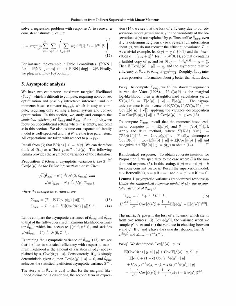
Figure 7 shows train and test accuracies as we makepasses over the dataset. Typically, after sufficiently manypasses, the marginal likelihood gains an advantage over themoment-based estimator. For small regions, we expect thebeam search approximation to be accurate, and indeed themarginal likelihood estimator is dominant there. For largerregions, the moment-based estimator (i) achieves high ac-curacy early and (ii) dominates for several passes beforethe marginal likelihood estimator overtakes it. Altogether,

2The (uncentered) R2 coefficient of parameters w in a linearregression with design X and labels Y is ‖Xw − Y ‖2/‖Y ‖2.

3We use the housing (mlcomp.org/datasets/840) andsongs (mlcomp.org/datasets/748) data from mlcomp.

4We used the Wall Street Journal portion of the Penn Tree-bank. Sections 0-21 comprise the training set and 22-24 are test.

5The dataset has 45 tag values. We use a beam of size 500after analytically marginalizing nodes outside the region.

mlcomp.org/datasets/840

mlcomp.org/datasets/748

http://mlcomp.org


..

1

.

2

.

3

.

4

.

5

.

6

.

7

.

8

.

0.6

.

0.7

.

0.8

.

0.9

.

1.0

.

fully supervised, train accuracy

.

1

.

2

.

3

.

4

.

5

.

6

.

7

.

8

.

0.6

.

0.7

.

0.8

.

0.9

.

1.0

.

fully supervised, test accuracy

.

1

.

2

.

3

.

4

.

5

.

6

.

7

.

8

.

0.6

.

0.7

.

0.8

.

0.9

.

1.0

.

window 1, train accuracy

.

MOM

.

Marg

.

1

.

2

.

3

.

4

.

5

.

6

.

7

.

8

.

0.6

.

0.7

.

0.8

.

0.9

.

1.0

.

window 1, test accuracy

.

MOM

.

Marg

.

1

.

2

.

3

.

4

.

5

.

6

.

7

.

8

.

0.6

.

0.7

.

0.8

.

0.9

.

1.0

.


.

MOM

.

Marg

.

1

.

2

.

3

.

4

.

5

.

6

.

7

.

8

.

0.6

.

0.7

.

0.8

.

0.9

.

1.0

.


.

MOM

.

Marg

.

1

.

2

.

3

.

4

.

5

.

6

.

7

.

8

.

0.6

.

0.7

.

0.8

.

0.9

.

1.0

.


.

MOM

.

Marg

.

1

.

2

.

3

.

4

.

5

.

6

.

7

.

8

.

0.6

.

0.7

.

0.8

.

0.9

.

1.0

.


.

MOM

.

Marg

.

1

.

2

.

3

.

4

.

5

.

6

.

7

.

8

.

0.6

.

0.7

.

0.8

.

0.9

.

1.0

.


.

MOM

.

Marg

.

1

.

2

.

3

.

4

.

5

.

6

.

7

.

8

.

0.6

.

0.7

.

0.8

.

0.9

.

1.0

.


.

MOM

.

Marg

.1

.2

.3

.4

.5

.6

.7

.8

.# passes

.

0.6

.

0.7

.

0.8

.

0.9

.

1.0

.


.

MOM

.

Marg

.1

.2

.3

.4

.5

.6

.7

.8

.# passes

.

0.6

.

0.7

.

0.8

.

0.9

.

1.0

.


.

MOM

.

Marg

Figure 7. Train and test per-position accuracies for θmarg andθmom on part-of-speech tagging, under various sized regions ofcount annotations, as training passes are taken through the dataset.

the experiment highlights that the moment-based estimatoris favorable in computationally-constrained settings.

8. Related work and discussionThis work was motivated by two use cases of indirect su-pervision: local privacy and cheap annotations. Each tradesoff statistical accuracy for another resource: privacy or an-notation cost. Local privacy has its roots in classical ran-domized response for conducting surveys (Warner, 1965),which has been extended to the multivariate (Tamhane,1981) and conditional (Matloff, 1984) settings. In the com-puter science community, differential privacy has emergedas a useful formalization of privacy (Dwork, 2006). Wework with the stronger notion of local differential privacy(Evfimievski et al., 2004; Kasiviswanathan et al., 2011;Duchi et al., 2013). Our contribution here is two-fold:First, we bring local privacy to the graphical model setting,which provides an opportunity for the privacy mechanismto be sensitive to the model structure. While we believe our

mechanisms are reasonable, an open question is designingoptimal mechanisms in the structured case. Second, weconnect privacy with other forms of indirect supervision.

The second use case is learning from lightweight annota-tions, which has taken many forms in the literature. Multi-instance learning (Oded & Tomas, 1998) is popular in com-puter vision, where it is natural to label the presence but notlocation of objects (Babenko et al., 2009). In natural lan-guage processing, there also been work on learning fromstructured outputs where, like this work, only counts of la-bels are observed (Mann & McCallum, 2008; Liang et al.,2009). However, these works resort to likelihood-based ap-proaches which involve non-convex optimization and ap-proximate inference, whereas in this work, we show thatlinear algebra and convex optimization suffice under mod-eling assumptions.

Quadrianto et al. (2008) showed how to learn from labelproportions of groups of examples, using a linear systemtechnique similar to ours. However, they assume that thegroup is conditionally independent of the example giventhe label, which would not apply in our region-based anno-tation setup since our regions contain arbitrarily correlatedinputs and heterogeneous labels. In return, we do need tomake the stronger assumption that each label y[i] dependsonly on a discrete x[i], so that the credit assignment can bedone using a linear program. An open challenge is to allowfor heterogeneity with complex inputs.

Indirect supervision arises more generally in latent-variablemodels, which arises in machine translation (Brown et al.,1993), semantic parsing (Liang et al., 2011), object detec-tion (Quattoni et al., 2004), and other missing data prob-lems in statistics (M & Naisyin, 2000). The indirect su-pervision problems in this paper have additional structure:we have an unknown model pθ and a known supervisionfunction S. It is this structure allows us to obtain computa-tionally efficient method of moments procedures.

We started this work to see how much juice we couldsqueeze out of just linear moment equations, and the an-swer is more than we expected. Of course, for moregeneral latent-variable models beyond linearly indirectly-supervised problems, we would need more powerful tools.In recent years, tensor factorization techniques have pro-vided efficient methods for a wide class of latent-variablemodels (Hsu et al., 2012; Anandkumar et al., 2012; Hsu& Kakade, 2013; Anandkumar et al., 2013; Chaganty &Liang, 2013; Halpern & Sontag, 2013; Chaganty & Liang,2014). One can leverage even more general polynomial-solving techniques to expand the set of models (Wang et al.,2015). In general, the method of moments allows us toleverage statistical structure to alleviate computational in-tractability, and we anticipate more future developmentsalong these lines.


Reproducibility. The code, data and experimentsfor this paper are available on Codalab at https://worksheets.codalab.org/worksheets/0x6a264a96efea41158847eef9ec2f76bc/.

ReferencesAnandkumar, A., Foster, D. P., Hsu, D., Kakade, S. M.,

and Liu, Y. Two SVDs suffice: Spectral decompositionsfor probabilistic topic modeling and latent Dirichlet al-location. In Advances in Neural Information ProcessingSystems (NIPS), 2012.

Anandkumar, A., Ge, R., Hsu, D., Kakade, S. M., and Tel-garsky, M. Tensor decompositions for learning latentvariable models. arXiv, 2013.

Babenko, B., Yang, M., and Belongie, S. Visual track-ing with online multiple instance learning. In ComputerVision and Pattern Recognition (CVPR), pp. 983–990,2009.

Brown, P. F., Pietra, S. A. D., Pietra, V. J. D., and Mercer,R. L. The mathematics of statistical machine transla-tion: Parameter estimation. Computational Linguistics,19:263–311, 1993.

Chaganty, A. and Liang, P. Spectral experts for estimatingmixtures of linear regressions. In International Confer-ence on Machine Learning (ICML), 2013.

Chaganty, A. and Liang, P. Estimating latent-variablegraphical models using moments and likelihoods. InInternational Conference on Machine Learning (ICML),2014.

Chang, M., Ratinov, L., and Roth, D. Guiding semi-supervision with constraint-driven learning. In Associa-tion for Computational Linguistics (ACL), pp. 280–287,2007.

Dempster, A. P., M., L. N., and B., R. D. Maximum likeli-hood from incomplete data via the EM algorithm. Jour-nal of the Royal Statistical Society: Series B, 39(1):1–38,1977.

Duchi, J. C., Jordan, M. I., and Wainwright, M. J. Localprivacy and statistical minimax rates. In Foundations ofComputer Science (FOCS), 2013.

Dwork, C. Differential privacy. In Automata, languagesand programming, pp. 1–12, 2006.

Dwork, C., McSherry, F., Nissim, K., and Smith, A. Cal-ibrating noise to sensitivity in private data analysis. InProceedings of the 3rd Theory of Cryptography Confer-ence, pp. 265–284, 2006.

Evfimievski, A., Srikant, R., Agrawal, R., and Gehrke, J.Privacy preserving mining of association rules. Informa-tion Systems, 29(4):343–364, 2004.

Graca, J., Ganchev, K., and Taskar, B. Expectation maxi-mization and posterior constraints. In Advances in Neu-ral Information Processing Systems (NIPS), pp. 569–576, 2008.

Haghighi, A. and Klein, D. Prototype-driven learningfor sequence models. In North American Associationfor Computational Linguistics (NAACL), pp. 320–327,2006.

Halpern, Y. and Sontag, D. Unsupervised learning of noisy-or Bayesian networks. In Uncertainty in Artificial Intel-ligence (UAI), 2013.

Hsu, D. and Kakade, S. M. Learning mixtures of sphericalGaussians: Moment methods and spectral decomposi-tions. In Innovations in Theoretical Computer Science(ITCS), 2013.

Hsu, D., Kakade, S. M., and Zhang, T. A spectral algorithmfor learning hidden Markov models. In Conference onLearning Theory (COLT), 2009.

Hsu, D., Kakade, S. M., and Liang, P. Identifiability andunmixing of latent parse trees. In Advances in NeuralInformation Processing Systems (NIPS), 2012.

Kasiviswanathan, S. P., Lee, H. K., Nissim, K., Raskhod-nikova, S., and Smith, A. What can we learn privately?SIAM Journal on Computing, 40(3):793–826, 2011.

Lafferty, J., McCallum, A., and Pereira, F. Conditionalrandom fields: Probabilistic models for segmenting andlabeling data. In International Conference on MachineLearning (ICML), pp. 282–289, 2001.

Liang, P., Jordan, M. I., and Klein, D. Learning from mea-surements in exponential families. In International Con-ference on Machine Learning (ICML), 2009.

Liang, P., Jordan, M. I., and Klein, D. Learningdependency-based compositional semantics. In Associa-tion for Computational Linguistics (ACL), pp. 590–599,2011.

M, R. J. and Naisyin, W. Inference for imputation estima-tors. Biometrika, 87(1):113–124, 2000.

Mann, G. and McCallum, A. Generalized expectation cri-teria for semi-supervised learning of conditional randomfields. In Human Language Technology and Associationfor Computational Linguistics (HLT/ACL), pp. 870–878,2008.

https://worksheets.codalab.org/worksheets/0x6a264a96efea41158847eef9ec2f76bc/




Matloff, N. S. Use of covariates in randomized responsesettings. Statistics & Probability Letters, 2(1):31–34,1984.

Oded, M. and Tomas, L. A framework for multiple-instance learning. Advances in neural information pro-cessing systems, pp. 570–576, 1998.

Pearson, K. Contributions to the mathematical theory ofevolution. Philosophical Transactions of the Royal So-ciety of London. A, 185:71–110, 1894.

Quadrianto, N., Smola, A. J., Caetano, T. S., and Le, Q. V.Estimating labels from label proportions. In Interna-tional Conference on Machine Learning (ICML), pp.776–783, 2008.

Quattoni, A., Collins, M., and Darrell, T. Conditional ran-dom fields for object recognition. In Advances in NeuralInformation Processing Systems (NIPS), 2004.

Steinhardt, J. and Liang, P. Learning with relaxed super-vision. In Advances in Neural Information ProcessingSystems (NIPS), 2015.

Tamhane, A. C. Randomized response techniques for mul-tiple sensitive attributes. Journal of the American Statis-tical Association (JASA), 76(376):916–923, 1981.

Vaish, R., Wyngarden, K., Chen, J., Cheung, B., and Bern-stein, M. S. Twitch crowdsourcing: crowd contributionsin short bursts of time. In Conference on Human Factorsin Computing Systems (CHI), pp. 3645–3654, 2014.

van der Vaart, A. W. Asymptotic statistics. CambridgeUniversity Press, 1998.

Wang, S., Chaganty, A., and Liang, P. Estimating mixturemodels via mixture of polynomials. In Advances in Neu-ral Information Processing Systems (NIPS), 2015.

Warner, S. L. Randomized response: A survey tech-nique for eliminating evasive answer bias. Journal ofthe American Statistical Association (JASA), 60(309):63–69, 1965.


A. Details of privacy schemesA.1. Local privacy using sufficient statistics

Proof of Proposition 1. Because φ is a sufficient statistic, by definition there exists some channel Q(y | φ(x, y)) and adistribution Fθ(φ(x, y) | x) such that pθ(y | x) = Q(y | φ(x, y))Fθ(φ(x, y) | x). If we define

S′(o | φ(x, y)) =∑y

S(o | y)Q(y | φ(x, y)), (18)

then (8) follows by substitution and algebra:

A.2. Privacy guarantees of proposed schemes

In order to show differential privacy of the two schemes proposed in Section 3, we first note that it suffices to havedifferential privacy of the observations o with respect to any (possibly random) data o ∈ O processed given the privatevariable y such that y → o→ o forms a Markov chain.

To see this, suppose Q is an α-differentially private channel taking the intermediate variable o to o and fix any x ∈ X . LetR(· | y) be the distribution of o given y ∈ Y . Now, for the end-to-end channel S,

supo,y,y′

S(o | y)

S(o | y′)= supo,y,y′

∑o∈O Q(o | o)R(o | y)∑o∈O Q(o | o)R(o | y′)

(19)

≤ supo,y,y′

maxoQ(o | o)minoQ(o | o)

(20)

≤ exp(α). (21)

Coordinate release. Recall that in the coordinate release mechanism, we first pick a coordinate j and release observationocr after flipping o[j] with probability exp(α2 )

1+exp(α2 ) .

Q(ocr, j | o)Q(ocr, j | o′)

= exp(α

2(|ocr − (1− o[j])| − |ocr − (1− o′[j])|)

)(22)

≤ exp(α), (23)

where the final step is by the triangle inequality applied twice.

Per-value φ-RR. Privacy of per-value φ-RR follows similarly.

Each coordinate of o is flipped with probability qαδ

=exp( α

2δ)

1+exp( α2δ

) , where δ is chosen such that δ ≤ ‖o‖1, ‖o′‖1 (see Section3.2)

Q(opv | o)Q(opv | o′)

= exp( α

2δ(‖opv − (1− o)‖1 − ‖opv − (1− o′)‖1)

)(24)

≤ exp(α). (25)

A.3. Variance of moments-based estimator for different privacy schemes.

For simplicity, we once again consider the unconditional case (where x is empty) and assume φ ∈ 0, 1d.

Theorem 1 (Asymptotic variance (coordinate release)). The asymptotic variance of θmom for α-differentially private coor-dinate release scheme, under a uniform coordinate sampling distribution pcr is

Σcrmom = I−1 + I−1HcrI−1,

where

Hcr =dqα(1− qα)

(2qα − 1)2I + E[ddiag(φ(y))2 − φ(y)⊗2], (26)


As in Lemma 1, the matrix Hcr governs the loss in efficiency under the coordinate release mechanism, which arises fromtwo sources: (i) variance due to the stochastic flipping process and (ii) variance due to choosing a random coordinate forrelease.

Proof. When pcr is uniform, the observation function βcr(j, ocr) takes the following form.

βcr(j, ocr) = docr − 1 + qα

2qα − 1ej .

From (14), we have that Hcr = E[Cov[βcr(j, ocr) | y]].

We decompose Cov[β(j, ocr) | y] as

E[Cov[β(j, ocr) | j, y] | y] + Cov[E[β(j, ocr) | j, y] | y]

=d2

(2qα − 1)2

(E[Cov[ocr ej | j, y] | y] + Cov[E[(ocr − 1 + qα) ej | j, y] | y]

)=

d2

(2qα − 1)2E[diag(qα(1− qα)ej) | y] +

d2

(2qα − 1)2Cov[[(2qα − 1)φ(y)[j] + 1− qα − 1 + qα]ej | y]

=d2

(2qα − 1)2E[diag(qα(1− qα)ej) | y] + d2 Cov[φ(y)[j]ej | y]

=dqα(1− qα)

(2qα − 1)2I + [ddiag(φ(y))2 − φ(y)⊗2],

Theorem 2 (Asymptotic variance (per-value φ-RR)). The asymptotic variance of θmom for α-differentially per-value φ-RR scheme is

Σpvmom = I−1 + I−1HpvI−1, (27)

Hpv =qα/δ(1− qα/δ)(2qα/δ − 1)2

I. (28)

Proof. From (9), we have

βpv(x, opv)def=

opv − 1 + qα/δ1

2qα/δ − 1.

From (14), we know that Hpv = E[Cov[βpv(opv) | y]] = 1(2qα/δ−1)2E[Cov[opv | y]].

Each entry opv[j] is chosen independently according to a Bernoulli distribution with parameter qα/δ (if o[i] = 1) or 1−qα/δ(if o[i] = 0), implying the claim.

A.4. Comparison of the two schemes

We use tr(Hcr) and tr(Hpv) to quantitatively estimate the loss in efficiency of Σmom under the two privacy schemes.

For small x, approximate qx = ex/2

1+ex/2 locally as 12 + x

8 (via Taylor expansion). Substituting in (26) and (28) gives thefollowing expressions for small α:

tr(Hcr) ≈ 4d2

α2+ δ(d− 1). (29)

tr(Hpv) ≈ 4dδ2

α2. (30)

When δ is constant (independent of d), tr(Hpv) grows linearly with d whereas tr(Hcr) grows quadratically with d. There-fore per-value φ-RR has smaller loss when φ has low l1 norm. Meanwhile, when δ = O(d), tr(Hpv) = O(d3) andtr(Hcr) = O(d2). Hence coordinate release is a more appealing choice if φ is dense.

estimation from indirect supervision with linear moments · estimation from indirect supervision...

Documents